Backfitting for large scale crossed random effects regressions

Abstract

Regression models with crossed random effect errors can be very expensive to compute. The cost of both generalized least squares and Gibbs sampling can easily grow as $N^{3/2}$ (or worse) for $N$ observations. Papaspiliopoulos et al., (2020) present a collapsed Gibbs sampler that costs $O(N)$, but under an extremely stringent sampling model. We propose a backfitting algorithm to compute a generalized least squares estimate and prove that it costs $O(N)$. A critical part of the proof is in ensuring that the number of iterations required is $O(1)$ which follows from keeping a certain matrix norm below $1-\delta$ for some $\delta>0$. Our conditions are greatly relaxed compared to those for the collapsed Gibbs sampler, though still strict. Empirically, the backfitting algorithm has a norm below $1-\delta$ under conditions that are less strict than those in our assumptions. We illustrate the new algorithm on a ratings data set from Stitch Fix.

1 Introduction

To estimate a regression when the errors have a non-identity covariance matrix, we usually turn first to generalized least squares (GLS). Somewhat surprisingly, GLS proves to be computationally challenging in the very simple setting of the unbalanced crossed random effects models that we study here. For that problem, the cost to compute the GLS estimate on $N$ data points grows at best like $O(N^{3/2})$ under the usual algorithms. If we additionally assume Gaussian errors, then Gao and Owen, (2019) show that even evaluating the likelihood one time costs at least a multiple of $N^{3/2}$. These costs make the usual algorithms for GLS infeasible for large data sets such as those arising in electronic commerce.

In this paper, we present an iterative algorithm based on a backfitting approach from Buja et al., (1989). This algorithm is known to converge to the GLS solution. The cost of each iteration is $O(N)$ and so we also study how the number of iterations grows with $N$.

The crossed random effects model we consider has

$$Y_{ij}=x_{ij}^{\mathsf{T}}\beta+a_{i}+b_{j}+e_{ij},\quad 1\leqslant i\leqslant R,\quad 1\leqslant j\leqslant C$$ (1)

for random effects $a_{i}$ and $b_{j}$ and an error $e_{ij}$ with a fixed effects regression parameter $\beta\in\mathbb{R}^{p}$ for the covariates $x_{ij}\in\mathbb{R}^{p}$. We assume that $a_{i}\stackrel{{\scriptstyle\mathrm{iid}}}{{\sim}}(0,\sigma^{2}_{A})$, $b_{j}\stackrel{{\scriptstyle\mathrm{iid}}}{{\sim}}(0,\sigma^{2}_{B})$, and $e_{ij}\stackrel{{\scriptstyle\mathrm{iid}}}{{\sim}}(0,\sigma^{2}_{E})$ are all independent. It is thus a mixed effects model in which the random portion has a crossed structure. The GLS estimate is also the maximum likelihood estimate (MLE), when $a_{i}$, $b_{j}$ and $e_{ij}$ are Gaussian. Because we assume that $p$ is fixed as $N$ grows, we often leave $p$ out of our cost estimates, giving instead the complexity in $N$.

The GLS estimate $\hat{\beta}_{\mathrm{GLS}}$ for crossed random effects can be efficiently estimated if all $R\times C$ values are available. Our motivating examples involve ratings data where $R$ people rate $C$ items and then it is usual that the data are very unbalanced with a haphazard observational pattern in which only $N\ll R\times C$ of the $(x_{ij},Y_{ij})$ pairs are observed. The crossed random effects setting is significantly more difficult than a hierarchical model with just $a_{i}+e_{ij}$ but no $b_{j}$ term. Then the observations for index $j$ are ‘nested within’ those for each level of index $i$. The result is that the covariance matrix of all observed $Y_{ij}$ values has a block diagonal structure allowing GLS to be computed in $O(N)$ time.

Hierarchical models are very well suited to Bayesian computation (Gelman and Hill,, 2006). Crossed random effects are a much greater challenge. Gao and Owen, (2017) find that the Gibbs sampler can take $O(N^{1/2})$ iterations to converge to stationarity, with each iteration costing $O(N)$ leading once again to $O(N^{3/2})$ cost. For more examples where the costs of solving equations versus sampling from a covariance attain the same rate see Goodman and Sokal, (1989) and Roberts and Sahu, (1997). As further evidence of the difficulty of this problem, the Gibbs sampler was one of nine MCMC algorithms that Gao and Owen, (2017) found to be unsatisfactory. Furthermore, Bates et al., (2015) removed the mcmcsamp function from the R package lme4 because it was considered unreliable even for the problem of sampling the posterior distribution of the parameters from previously fitted models, and even for those with random effects variances near zero.

Papaspiliopoulos et al., (2020) present an exception to the high cost of a Bayesian approach for crossed random effects. They propose a collapsed Gibbs sampler that can potentially mix in $O(1)$ iterations. To prove this rate, they make an extremely stringent assumption that every index $i=1,\dots,R$ appears in the same number $N/C$ of observed data points and similarly every $j=1,\dots,C$ appears in $N/R$ data points. Such a condition is tantamount to requiring a designed experiment for the data and it is much stronger than what their algorithm seems to need in practice. Under that condition their mixing rate asymptotes to a quantity $\rho_{\mathrm{aux}}$, described in our discussion section, that in favorable circumstances is $O(1)$. They find empirically that their sampler has a cost that scales well in many data sets where their balance condition does not hold.

In this paper we study an iterative linear operation, known as backfitting, for GLS. Each iteration costs $O(N)$. The speed of convergence depends on a certain matrix norm of that iteration, which we exhibit below. If the norm remains bounded strictly below $1$ as $N\to\infty$, then the number of iterations to convergence is $O(1)$. We are able to show that the matrix norm is $O(1)$ with probability tending to one, under conditions where the number of observations per row (or per column) is random and even the expected row or column counts may vary, though in a narrow range. While this is a substantial weakening of the conditions in Papaspiliopoulos et al., (2020), it still fails to cover many interesting cases. Like them, we find empirically that our algorithm scales much more broadly than under the conditions for which scaling is proved.

We suspect that the computational infeasibility of GLS leads many users to use ordinary least squares (OLS) instead. OLS has two severe problems. First, it is inefficient with $\mathrm{var}(\hat{\beta}_{\mathrm{OLS}})$ larger than $\mathrm{var}(\hat{\beta}_{\mathrm{GLS}})$. This is equivalent to OLS ignoring some possibly large fraction of the information in the data. Perhaps more seriously, OLS is naive. It produces an estimate of $\mathrm{var}(\hat{\beta}_{\mathrm{OLS}})$ that can be too small by a large factor. That amounts to overestimating the quantity of information behind $\hat{\beta}_{\mathrm{OLS}}$, also by a potentially large factor.

The naivete of OLS can be countered by using better variance estimates. One can bootstrap it by resampling the row and column entities as in Owen, (2007). There is also a version of Huber-White variance estimation for this case in econometrics. See for instance Cameron et al., (2011). While these methods counter the naivete of OLS, the inefficiency of OLS remains.

The method of moments algorithm in Gao and Owen, (2019) gets consistent asymptotically normal estimates of $\beta$, $\sigma^{2}_{A}$, $\sigma^{2}_{B}$ and $\sigma^{2}_{E}$. It produces a GLS estimate $\hat{\beta}$ that is more efficient than OLS but still not fully efficient because it accounts for correlations due to only one of the two crossed random effects. While inefficient, it is not naive because its estimate of $\mathrm{var}(\hat{\beta})$ properly accounts for variance due to $a_{i}$, $b_{j}$ and $e_{ij}$.

In this paper we get a GLS estimate $\hat{\beta}$ that takes account of all three variance components, making it efficient. We also provide an estimate of $\mathrm{var}(\hat{\beta})$ that accounts for all three components, so our estimate is not naive. Our algorithm requires consistent estimates of the variance components $\sigma^{2}_{A}$, $\sigma^{2}_{B}$ and $\sigma^{2}_{E}$ in computing $\hat{\beta}$ and $\widehat{\mathrm{var}}(\hat{\beta})$. We use the method of moments estimators from Gao and Owen, (2017) that can be computed in $O(N)$ work. By Gao and Owen, (2017, Theorem 4.2), these estimates of $\sigma^{2}_{A}$, $\sigma^{2}_{B}$ and $\sigma^{2}_{E}$ are asymptotically uncorrelated and each of them has the same asymptotic variance it would have had were the other two variance components equal to zero. It is not known whether they are optimally estimated, much less optimal subject to an $O(N)$ cost constraint. The variance component estimates are known to be asymptotically normal (Gao,, 2017).

The rest of this paper is organized as follows. Section 2 introduces our notation and assumptions for missing data. Section 3 presents the backfitting algorithm from Buja et al., (1989). That algorithm was defined for smoothers, but we are able to cast the estimation of random effect parameters as a special kind of smoother. Section 4 proves our result about backfitting being convergent with a probability tending to one as the problem size increases. Section 5 shows numerical measures of the matrix norm of the backfitting operator. It remains bounded below and away from one under more conditions than our theory shows. We find that even one iteration of the lmer function in lme4 package Bates et al., (2015) has a cost that grows like $N^{3/2}$ in one setting and like $N^{2.1}$ in another, sparser one. The backfitting algorithm has cost $O(N)$ in both of these cases. Section 6 illustrates our GLS algorithm on some data provided to us by Stitch Fix. These are customer ratings of items of clothing on a ten point scale. Section 7 has a discussion of these results. An appendix contains some regression output for the Stitch Fix data.

2 Missingness

We adopt the notation from Gao and Owen, (2019). We let $Z_{ij}\in\{0,1\}$ take the value $1$ if $(x_{ij},Y_{ij})$ is observed and $0$ otherwise, for $i=1,\dots,R$ and $j=1,\dots,C$. In many of the contexts we consider, the missingness is not at random and is potentially informative. Handling such problems is outside the scope of this paper, apart from a brief discussion in Section 7. It is already a sufficient challenge to work without informative missingness.

The matrix $Z\in\{0,1\}^{R\times C}$, with elements $Z_{ij}$ has $N_{i\text{\tiny$\bullet$}}=\sum_{j=1}^{C}Z_{ij}$ observations in ‘row $i$’ and $N_{\text{\tiny$\bullet$}j}=\sum_{i=1}^{R}Z_{ij}$ observations in ‘column $j$’. We often drop the limits of summation so that $i$ is always summed over $1,\dots,R$ and $j$ over $1,\dots,C$. When we need additional symbols for row and column indices we use $r$ for rows and $s$ for columns. The total sample size is $N=\sum_{i}\sum_{j}Z_{ij}=\sum_{i}N_{i\text{\tiny$\bullet$}}=\sum_{j}N_{\text{\tiny$\bullet$}j}$.

There are two co-observation matrices, $Z^{\mathsf{T}}Z$ and $ZZ^{\mathsf{T}}$. Here $(Z^{\mathsf{T}}Z)_{js}=\sum_{i}Z_{ij}Z_{is}$ gives the number of rows in which data from both columns $j$ and $s$ were observed, while $(ZZ^{\mathsf{T}})_{ir}=\sum_{j}Z_{ij}Z_{rj}$ gives the number of columns in which data from both rows $i$ and $r$ were observed.

In our regression models, we treat $Z_{ij}$ as nonrandom. We are conditioning on the actual pattern of observations in our data. When we study the rate at which our backfitting algorithm converges, we consider $Z_{ij}$ drawn at random. That is, the analyst is solving a GLS conditionally on the pattern of observations and missingness, while we study the convergence rates that analyst will see for data drawn from a missingness mechanism defined in Section 4.2.

If we place all of the $Y_{ij}$ into a vector $\mathcal{Y}\in\mathbb{R}^{N}$ and $x_{ij}$ compatibly into a matrix $\mathcal{X}\in\mathbb{R}^{N\times p}$, then the naive and inefficient OLS estimator is

$$\hat{\beta}_{\mathrm{OLS}}=(\mathcal{X}^{\mathsf{T}}\mathcal{X})^{-1}\mathcal{X}^{\mathsf{T}}\mathcal{Y}.$$ (2)

This can be computed in $O(Np^{2})$ work. We prefer to use the GLS estimator

$$\hat{\beta}_{\mathrm{GLS}}=(\mathcal{X}^{\mathsf{T}}\mathcal{V}^{-1}\mathcal{X})^{-1}\mathcal{X}^{\mathsf{T}}\mathcal{V}^{-1}\mathcal{Y},$$ (3)

where $\mathcal{V}\in\mathbb{R}^{N\times N}$ contains all of the $\mathrm{cov}(Y_{ij},Y_{rs})$ in an ordering compatible with $\mathcal{X}$ and $\mathcal{Y}$. A naive algorithm costs $O(N^{3})$ to solve for $\hat{\beta}_{\mathrm{GLS}}$. It can actually be solved through a Cholesky decomposition of an $(R+C)\times(R+C)$ matrix (Searle et al.,, 1992). That has cost $O(R^{3}+C^{3})$. Now $N\leqslant RC$, with equality only for completely observed data. Therefore $\max(R,C)\geqslant\sqrt{N}$, and so $R^{3}+C^{3}\geqslant N^{3/2}$. When the data are sparsely enough observed it is possible that $\min(R,C)$ grows more rapidly than $N^{1/2}$. In a numerical example in Section 5 we have $\min(R,C)$ growing like $N^{0.70}$. In a hierarchical model, with $a_{i}$ but no $b_{j}$ we would find $\mathcal{V}$ to be block diagonal and then $\hat{\beta}_{\mathrm{GLS}}$ could be computed in $O(N)$ work.

A reviewer reminds us that it has been known since Strassen, (1969) that systems of equations can be solved more quickly than cubic time. Despite that, current software is still dominated by cubic time algorithms. Also none of the known solutions are quadratic and so in our setting the cost would be at least a multiple of $(R+C)^{2+\gamma}$ for some $\gamma>0$ and hence not $O(N)$.

We can write our crossed effects model as

$$\mathcal{Y}=\mathcal{X}\beta+\mathcal{Z}_{A}\boldsymbol{a}+\mathcal{Z}_{B}\boldsymbol{b}+\boldsymbol{e}$$ (4)

for matrices $\mathcal{Z}_{A}\in\{0,1\}^{N\times R}$ and $\mathcal{Z}_{B}\in\{0,1\}^{N\times C}$. The $i$’th column of $\mathcal{Z}_{A}$ has ones for all of the $N$ observations that come from row $i$ and zeroes elsewhere. The definition of $\mathcal{Z}_{B}$ is analogous. The observation matrix can be written $Z=\mathcal{Z}_{A}^{\mathsf{T}}\mathcal{Z}_{B}$. The vector $\boldsymbol{e}$ has all $N$ values of $e_{ij}$ in compatible order. Vectors $\boldsymbol{a}$ and $\boldsymbol{b}$ contain the row and column random effects $a_{i}$ and $b_{j}$. In this notation

$$\mathcal{V}=\mathcal{Z}_{A}\mathcal{Z}_{A}^{\mathsf{T}}\sigma^{2}_{A}+\mathcal{Z}_{B}\mathcal{Z}_{B}^{\mathsf{T}}\sigma^{2}_{B}+I_{N}\sigma^{2}_{E},$$ (5)

where $I_{N}$ is the $N\times N$ identity matrix.

Our main computational problem is to get a value for $\mathcal{U}=\mathcal{V}^{-1}\mathcal{X}\in\mathbb{R}^{N\times p}$. To do that we iterate towards a solution $\boldsymbol{u}\in\mathbb{R}^{N}$ of $\mathcal{V}\boldsymbol{u}=\boldsymbol{x}$, where $\boldsymbol{x}\in\mathbb{R}^{N}$ is one of the $p$ columns of $\mathcal{X}$. After that, finding

$$\hat{\beta}_{\mathrm{GLS}}=(\mathcal{X}^{\mathsf{T}}\mathcal{U})^{-1}(\mathcal{Y}^{\mathsf{T}}\mathcal{U})^{\mathsf{T}}$$ (6)

is not expensive, because $\mathcal{X}^{\mathsf{T}}\mathcal{U}\in\mathbb{R}^{p\times p}$ and we suppose that $p$ is not large.

If the data ordering in $\mathcal{Y}$ and elsewhere sorts by index $i$, breaking ties by index $j$, then $\mathcal{Z}_{A}\mathcal{Z}_{A}^{\mathsf{T}}\in\{0,1\}^{N\times N}$ is a block matrix with $R$ blocks of ones of size $N_{i\text{\tiny$\bullet$}}\times N_{i\text{\tiny$\bullet$}}$ along the diagonal and zeroes elsewhere. The matrix $\mathcal{Z}_{B}\mathcal{Z}_{B}^{\mathsf{T}}$ will not be block diagonal in that ordering. Instead $P\mathcal{Z}_{B}\mathcal{Z}_{B}^{\mathsf{T}}P^{\mathsf{T}}$ will be block diagonal with $N_{\text{\tiny$\bullet$}j}\times N_{\text{\tiny$\bullet$}j}$ blocks of ones on the diagonal, for a suitable $N\times N$ permutation matrix $P$.

3 Backfitting algorithms

Our first goal is to develop computationally efficient ways to solve the GLS problem (6) for the linear mixed model (4). We use the backfitting algorithm that Hastie and Tibshirani, (1990) and Buja et al., (1989) use to fit additive models. We write $\mathcal{V}$ in (5) as $\sigma^{2}_{E}\left(\mathcal{Z}_{A}\mathcal{Z}_{A}^{\mathsf{T}}/\lambda_{A}+\mathcal{Z}_{B}\mathcal{Z}_{B}^{\mathsf{T}}/\lambda_{B}+I_{N}\right)$ with $\lambda_{A}=\sigma^{2}_{E}/\sigma^{2}_{A}$ and $\lambda_{B}=\sigma^{2}_{E}/\sigma^{2}_{B}$, and define $\mathcal{W}=\sigma^{2}_{E}\mathcal{V}^{-1}$. Then the GLS estimate of $\beta$ is

$$\hat{\beta}_{\mathrm{GLS}} =\arg\min_{\beta}(\mathcal{Y}-\mathcal{X}\beta)^{\mathsf{T}}\mathcal{W}(\mathcal{Y}-\mathcal{X}\beta)=(\mathcal{X}^{\mathsf{T}}\mathcal{W}\mathcal{X})^{-1}\mathcal{X}^{\mathsf{T}}\mathcal{W}\mathcal{Y}$$ (7)

and $\mathrm{cov}(\hat{\beta}_{\mathrm{GLS}})=\sigma^{2}_{E}(\mathcal{X}^{\mathsf{T}}\mathcal{W}\mathcal{X})^{-1}$.

It is well known (e.g., Robinson, (1991)) that we can obtain $\hat{\beta}_{\mathrm{GLS}}$ by solving the following penalized least-squares problem

$$\min_{\beta,\boldsymbol{a},\boldsymbol{b}}\|\mathcal{Y}-\mathcal{X}\beta-\mathcal{Z}_{A}\boldsymbol{a}-\mathcal{Z}_{B}\boldsymbol{b}\|^{2}+\lambda_{A}\|\boldsymbol{a}\|^{2}+\lambda_{B}\|\boldsymbol{b}\|^{2}.$$ (8)

Then $\hat{\beta}=\hat{\beta}_{\mathrm{GLS}}$ and $\hat{\boldsymbol{a}}$ and $\hat{\boldsymbol{b}}$ are the best linear unbiased prediction (BLUP) estimates of the random effects. This derivation works for any number of factors, but it is instructive to carry it through initially for one.

3.1 One factor

For a single factor, we simply drop the $\mathcal{Z}_{B}\boldsymbol{b}$ term from (4) to get

$$\mathcal{Y}=\mathcal{X}\beta+\mathcal{Z}_{A}\boldsymbol{a}+\boldsymbol{e}.$$

Then $\mathcal{V}=\mathrm{cov}(\mathcal{Z}_{A}\boldsymbol{a}+\boldsymbol{e})=\sigma^{2}_{A}\mathcal{Z}_{A}\mathcal{Z}_{A}^{\mathsf{T}}+\sigma^{2}_{E}I_{N}$, and $\mathcal{W}=\sigma^{2}_{E}\mathcal{V}^{-1}$ as before. The penalized least squares problem is to solve

$$\min_{\beta,\boldsymbol{a}}\|\mathcal{Y}-\mathcal{X}\beta-\mathcal{Z}_{A}\boldsymbol{a}\|^{2}+\lambda_{A}\|\boldsymbol{a}\|^{2}.$$ (9)

We show the details as we need them for a later derivation.

The normal equations from (9) yield

$$\boldsymbol{0} =\mathcal{X}^{\mathsf{T}}(\mathcal{Y}-\mathcal{X}\hat{\beta}-\mathcal{Z}_{A}\hat{\boldsymbol{a}}),\quad\text{and}$$ (10)

$$\boldsymbol{0} =\mathcal{Z}_{A}^{\mathsf{T}}(\mathcal{Y}-\mathcal{X}\hat{\beta}-\mathcal{Z}_{A}\hat{\boldsymbol{a}})-\lambda_{A}\hat{\boldsymbol{a}}.$$ (11)

Solving (11) for $\hat{\boldsymbol{a}}$ and multiplying the solution by $\mathcal{Z}_{A}$ yields

$$\mathcal{Z}_{A}\hat{\boldsymbol{a}}=\mathcal{Z}_{A}(\mathcal{Z}_{A}^{\mathsf{T}}\mathcal{Z}_{A}+\lambda_{A}I_{R})^{-1}\mathcal{Z}_{A}^{\mathsf{T}}(\mathcal{Y}-\mathcal{X}\hat{\beta})\equiv\mathcal{S}_{A}(\mathcal{Y}-\mathcal{X}\hat{\beta}),$$

for an $N\times N$ ridge regression “smoother matrix” $\mathcal{S}_{A}$. As we explain below this smoother matrix implements shrunken within-group means. Then substituting $\mathcal{Z}_{A}\hat{\boldsymbol{a}}$ into equation (10) yields

$$\hat{\beta}=(\mathcal{X}^{\mathsf{T}}(I_{N}-\mathcal{S}_{A})\mathcal{X})^{-1}\mathcal{X}^{\mathsf{T}}(I_{N}-\mathcal{S}_{A})\mathcal{Y}.$$ (12)

Using the Sherman-Morrison-Woodbury (SMW) identity, one can show that $\mathcal{W}=I_{N}-\mathcal{S}_{A}$ and hence $\hat{\beta}$ above equals $\hat{\beta}_{\mathrm{GLS}}$ from (7). This is not in itself a new discovery; see for example Robinson, (1991) or Hastie and Tibshirani, (1990) (Section 5.3.3).

To compute the solution in (12), we need to compute $\mathcal{S}_{A}\mathcal{Y}$ and $\mathcal{S}_{A}\mathcal{X}$. The heart of the computation in $\mathcal{S}_{A}\mathcal{Y}$ is $(\mathcal{Z}_{A}^{\mathsf{T}}\mathcal{Z}_{A}+\lambda_{A}I_{R})^{-1}\mathcal{Z}_{A}^{\mathsf{T}}\mathcal{Y}$. But $\mathcal{Z}_{A}^{\mathsf{T}}\mathcal{Z}_{A}=\mathrm{diag}(N_{1\text{\tiny$\bullet$}},N_{2\text{\tiny$\bullet$}},\ldots,N_{R\text{\tiny$\bullet$}})$ and we see that all we are doing is computing an $R$-vector of shrunken means of the elements of $\mathcal{Y}$ at each level of the factor $A$; the $i$th element is $\sum_{j}Z_{ij}Y_{ij}/(N_{i\text{\tiny$\bullet$}}+\lambda_{A})$. This involves a single pass through the $N$ elements of $Y$, accumulating the sums into $R$ registers, followed by an elementwise scaling of the $R$ components. Then pre-multiplication by $\mathcal{Z}_{A}$ simply puts these $R$ shrunken means back into an $N$-vector in the appropriate positions. The total cost is $O(N)$. Likewise $\mathcal{S}_{A}\mathcal{X}$ does the same separately for each of the columns of $\mathcal{X}$. Hence the entire computational cost for (12) is $O(Np^{2})$, the same order as regression on $\mathcal{X}$.

What is also clear is that the indicator matrix $\mathcal{Z}_{A}$ is not actually needed here; instead all we need to carry out these computations is the factor vector $f_{A}$ that records the level of factor $A$ for each of the $N$ observations. In the R language (R Core Team,, 2015) the following pair of operations does the computation:

  hat_a = tapply(y,fA,sum)/(table(fA)+lambdaA)
  hat_y = hat_a[fA]

where fA is a categorical variable (factor) $f_{A}$ of length $N$ containing the row indices $i$ in an order compatible with $Y\in\mathbb{R}^{N}$ (represented as y) and lambdaA is $\lambda_{A}=\sigma^{2}_{A}/\sigma^{2}_{E}$.

3.2 Two factors

With two factors we face the problem of incompatible block diagonal matrices discussed in Section 2. Define $\mathcal{Z}_{G}=(\mathcal{Z}_{A}\!:\!\mathcal{Z}_{B})$ ($R+C$ columns), $\mathcal{D}_{\lambda}=\mathrm{diag}(\lambda_{A}I_{R},\lambda_{B}I_{C})$, and $\boldsymbol{g}^{\mathsf{T}}=(\boldsymbol{a}^{\mathsf{T}},\boldsymbol{b}^{\mathsf{T}})$. Then solving (8) is equivalent to

$$\min_{\beta,\boldsymbol{g}}\|\mathcal{Y}-\mathcal{X}\beta-\mathcal{Z}_{G}\boldsymbol{g}\|^{2}+\boldsymbol{g}^{\mathsf{T}}\mathcal{D}_{\lambda}\boldsymbol{g}.$$ (13)

A derivation similar to that used in the one-factor case gives

$$\hat{\beta}=H_{\mathrm{GLS}}\mathcal{Y}\quad\text{for}\quad H_{\mathrm{GLS}}=(\mathcal{X}^{\mathsf{T}}(I_{N}-\mathcal{S}_{G})\mathcal{X})^{-1}\mathcal{X}^{\mathsf{T}}(I_{N}-\mathcal{S}_{G}),$$ (14)

where the hat matrix $H_{\mathrm{GLS}}$ is written in terms of a smoother matrix

$$\mathcal{S}_{G}=\mathcal{Z}_{G}(\mathcal{Z}_{G}^{\mathsf{T}}\mathcal{Z}_{G}+\mathcal{D}_{\lambda})^{-1}\mathcal{Z}_{G}^{\mathsf{T}}.$$ (15)

We can again use SMW to show that $I_{N}-\mathcal{S}_{G}=\mathcal{W}$ and hence the solution $\hat{\beta}=\hat{\beta}_{\mathrm{GLS}}$ in (7). But in applying $\mathcal{S}_{G}$ we do not enjoy the computational simplifications that occurred in the one factor case, because

$$\mathcal{Z}_{G}^{\mathsf{T}}\mathcal{Z}_{G}=\left(\begin{array}[]{cc}\mathcal{Z}_{A}^{\mathsf{T}}\mathcal{Z}_{A}&\mathcal{Z}_{A}^{\mathsf{T}}\mathcal{Z}_{B}\\[1.07639pt] \mathcal{Z}_{B}^{\mathsf{T}}\mathcal{Z}_{A}&\mathcal{Z}_{B}^{\mathsf{T}}\mathcal{Z}_{B}\end{array}\right)=\begin{pmatrix}\mathrm{diag}(N_{i\text{\tiny$\bullet$}})&Z\\ Z^{\mathsf{T}}&\mathrm{diag}(N_{\text{\tiny$\bullet$}j})\end{pmatrix},$$

where $Z\in\{0,1\}^{R\times C}$ is the observation matrix which has no special structure. Therefore we need to invert an $(R+C)\times(R+C)$ matrix to apply $\mathcal{S}_{G}$ and hence to solve (14), at a cost of at least $O(N^{3/2})$ (see Section 2).

Rather than group $\mathcal{Z}_{A}$ and $\mathcal{Z}_{B}$, we keep them separate, and develop an algorithm to apply the operator $\mathcal{S}_{G}$ efficiently. Consider a generic response vector $\mathcal{R}$ (such as $\mathcal{Y}$ or a column of $\mathcal{X}$) and the optimization problem

$$\min_{\boldsymbol{a},\boldsymbol{b}}\|\mathcal{R}-\mathcal{Z}_{A}\boldsymbol{a}-\mathcal{Z}_{B}\boldsymbol{b}\|^{2}+\lambda_{A}\|\boldsymbol{a}\|^{2}+\lambda_{B}\|\boldsymbol{b}\|^{2}.$$ (16)

Using $\mathcal{S}_{G}$ defined at (15) in terms of the indicator variables $\mathcal{Z}_{G}\in\{0,1\}^{N\times(R+C)}$ it is clear that the fitted values are given by $\widehat{\mathcal{R}}=\mathcal{S}_{G}\mathcal{R}$. Solving (16) would result in two blocks of estimating equations similar to equations (10) and (11). These can be written

$$\begin{split}\mathcal{Z}_{A}\hat{\boldsymbol{a}}&=\mathcal{S}_{A}(\mathcal{R}-\mathcal{Z}_{B}\hat{\boldsymbol{b}}),\quad\text{and}\\ \mathcal{Z}_{B}\hat{\boldsymbol{b}}&=\mathcal{S}_{B}(\mathcal{R}-\mathcal{Z}_{A}\hat{\boldsymbol{a}}),\end{split}$$ (17)

where $\mathcal{S}_{A}=\mathcal{Z}_{A}(\mathcal{Z}_{A}^{\mathsf{T}}\mathcal{Z}_{A}+\lambda_{A}I_{R})^{-1}\mathcal{Z}_{A}^{\mathsf{T}}$ is again the ridge regression smoothing matrix for row effects and similarly $\mathcal{S}_{B}=\mathcal{Z}_{B}(\mathcal{Z}_{B}^{\mathsf{T}}\mathcal{Z}_{B}+\lambda_{B}I_{C})^{-1}\mathcal{Z}_{B}^{\mathsf{T}}$ the smoothing matrix for column effects. We solve these equations iteratively by block coordinate descent, also known as backfitting. The iterations converge to the solution of (16) (Buja et al.,, 1989; Hastie and Tibshirani,, 1990).

It is evident that $\mathcal{S}_{A},\mathcal{S}_{B}\in\mathbb{R}^{N\times N}$ are both symmetric matrices. It follows that the limiting smoother $\mathcal{S}_{G}$ formed by combining them is also symmetric. See Hastie and Tibshirani, (1990, page 120). We will need this result later for an important computational shortcut.

Here the simplifications we enjoyed in the one-factor case once again apply. Each step applies its operator to a vector (the terms in parentheses on the right hand side in (17)). For both $\mathcal{S}_{A}$ and $\mathcal{S}_{B}$ these are simply the shrunken-mean operations described for the one-factor case, separately for factor $A$ and $B$ each time. As before, we do not need to actually construct $\mathcal{Z}_{B}$, but simply use a factor $f_{B}$ that records the level of factor $B$ for each of the $N$ observations.

The above description holds for a generic response $\mathcal{R}$; we apply that algorithm (in parallel) to $\mathcal{Y}$ and each column of $\mathcal{X}$ to obtain the quantities $\mathcal{S}_{G}\mathcal{X}$ and $\mathcal{S}_{G}\mathcal{Y}$ that we need to compute $H_{\mathrm{GLS}}\mathcal{Y}$ in (14). Now solving (14) is $O(Np^{2})$ plus a negligible $O(p^{3})$ cost. These computations deliver $\hat{\beta}_{\mathrm{GLS}}$; if the BLUP estimates $\hat{\boldsymbol{a}}$ and $\hat{\boldsymbol{b}}$ are also required, the same algorithm can be applied to the response $\mathcal{Y}-\mathcal{X}\hat{\beta}_{\mathrm{GLS}}$, retaining the $\boldsymbol{a}$ and $\boldsymbol{b}$ at the final iteration. We can also write

$$\mathrm{cov}(\hat{\beta}_{\mathrm{GLS}})=\sigma^{2}_{E}(\mathcal{X}^{\mathsf{T}}(I_{N}-\mathcal{S}_{G})\mathcal{X})^{-1}.$$ (18)

It is also clear that we can trivially extend this approach to accommodate any number of factors.

3.3 Centered operators

The matrices $\mathcal{Z}_{A}$ and $\mathcal{Z}_{B}$ both have row sums all ones, since they are factor indicator matrices (“one-hot encoders”). This creates a nontrivial intersection between their column spaces, and that of $\mathcal{X}$ since we always include an intercept, that can cause backfitting to converge more slowly. In this section we show how to counter this intersection of column spaces to speed convergence. We work with this two-factor model

$$\min_{\beta,\boldsymbol{a},\boldsymbol{b}}\|\mathcal{Y}-\mathcal{X}\beta-\mathcal{Z}_{A}\boldsymbol{a}-\mathcal{Z}_{B}\boldsymbol{b}\|^{2}+\lambda_{A}\|\boldsymbol{a}\|^{2}+\lambda_{B}\|\boldsymbol{b}\|^{2}.$$ (19)

Lemma 1.

If $\mathcal{X}$ in model (19) includes a column of ones (intercept), and $\lambda_{A}>0$ and $\lambda_{B}>0$, then the solutions for $\boldsymbol{a}$ and $\boldsymbol{b}$ satisfy $\sum_{i=1}^{R}a_{i}=0$ and $\sum_{j=1}^{C}b_{j}=0$.

Proof.

It suffices to show this for one factor and with $\mathcal{X}=\mathbf{1}$. The objective is now

$$\min_{\beta,\boldsymbol{a}}\|\mathcal{Y}-\mathbf{1}\beta-\mathcal{Z}_{A}\boldsymbol{a}\|^{2}+\lambda_{A}\|\boldsymbol{a}\|^{2}.$$ (20)

Notice that for any candidate solution $(\beta,\{a_{i}\}_{1}^{R})$, the alternative solution $(\beta+c,\{a_{i}-c\}_{1}^{R})$ leaves the loss part of (20) unchanged, since the row sums of $\mathcal{Z}_{A}$ are all one. Hence if $\lambda_{A}>0$, we would always improve $\boldsymbol{a}$ by picking $c$ to minimize the penalty term $\sum_{i=1}^{R}(a_{i}-c)^{2}$, or $c=(1/R)\sum_{i=1}^{R}a_{i}$. ∎

It is natural then to solve for $\boldsymbol{a}$ and $\boldsymbol{b}$ with these constraints enforced, instead of waiting for them to simply emerge in the process of iteration.

Theorem 1.

Consider the generic optimization problem

$$\min_{\boldsymbol{a}}\|\mathcal{R}-\mathcal{Z}_{A}\boldsymbol{a}\|^{2}+\lambda_{A}\|\boldsymbol{a}\|^{2}\quad\mbox{subject to }\sum_{i=1}^{R}a_{i}=0.$$ (21)

Define the partial sum vector $\mathcal{R}^{+}=\mathcal{Z}_{A}^{\mathsf{T}}\mathcal{R}$ with components $\mathcal{R}^{+}_{i}=\sum_{j}Z_{ij}\mathcal{R}_{ij}$, and let

$$w_{i}=\frac{(N_{i\text{\tiny$\bullet$}}+\lambda)^{-1}}{\sum_{r}(N_{r\text{\tiny$\bullet$}}+\lambda)^{-1}}.$$

Then the solution $\hat{\boldsymbol{a}}$ is given by

$$\hat{a}_{i}=\frac{\mathcal{R}^{+}_{i}-\sum_{r}w_{r}\mathcal{R}^{+}_{r}}{N_{i\text{\tiny$\bullet$}}+\lambda_{A}},\quad i=1,\ldots,R.$$ (22)

Moreover, the fit is given by

$$\mathcal{Z}_{A}\hat{\boldsymbol{a}}=\tilde{\mathcal{S}}_{A}\mathcal{R},$$

where $\tilde{\mathcal{S}}_{A}$ is a symmetric operator.

The computations are a simple modification of the non-centered case.

Proof.

Let $M$ be an $R\times R$ orthogonal matrix with first column $\mathbf{1}/\sqrt{R}$. Then $\mathcal{Z}_{A}\boldsymbol{a}=\mathcal{Z}_{A}MM^{\mathsf{T}}\boldsymbol{a}=\tilde{\mathcal{G}}\tilde{\boldsymbol{\gamma}}$ for $\mathcal{G}=\mathcal{Z}_{A}M$ and $\tilde{\boldsymbol{\gamma}}=M^{\mathsf{T}}\boldsymbol{a}$. Reparametrizing in this way leads to the equivalent problem

$$\min_{\tilde{\boldsymbol{\gamma}}}\|\mathcal{R}-\tilde{\mathcal{G}}\tilde{\boldsymbol{\gamma}}\|^{2}+\lambda_{A}\|\tilde{\boldsymbol{\gamma}}\|^{2},\quad\mbox{subject to }\tilde{\gamma}_{1}=0.$$ (23)

To solve (23), we simply drop the first column of $\tilde{\mathcal{G}}$. Let $\mathcal{G}=\mathcal{Z}_{A}Q$ where $Q$ is the matrix $M$ omitting the first column, and $\boldsymbol{\gamma}$ the corresponding subvector of $\tilde{\boldsymbol{\gamma}}$ having $R-1$ components. We now solve

$$\min_{\tilde{\boldsymbol{\gamma}}}\|\mathcal{R}-\mathcal{G}\boldsymbol{\gamma}\|^{2}+\lambda_{A}\|\tilde{\boldsymbol{\gamma}}\|^{2}$$ (24)

with no constraints, and the solution is $\hat{\boldsymbol{\gamma}}=(\mathcal{G}^{\mathsf{T}}\mathcal{G}+\lambda_{A}I_{R-1})^{-1}\mathcal{G}^{\mathsf{T}}\mathcal{R}$. The fit is given by $\mathcal{G}\hat{\boldsymbol{\gamma}}=\mathcal{G}(\mathcal{G}^{\mathsf{T}}\mathcal{G}+\lambda_{A}I_{R-1})^{-1}\mathcal{G}^{\mathsf{T}}\mathcal{R}=\tilde{\mathcal{S}}_{A}\mathcal{R}$, and $\tilde{\mathcal{S}}_{A}$ is clearly a symmetric operator.

To obtain the simplified expression for $\hat{\boldsymbol{a}}$, we write

$$\mathcal{G}\hat{\gamma} =\mathcal{Z}_{A}Q(Q^{\mathsf{T}}\mathcal{Z}_{A}^{\mathsf{T}}\mathcal{Z}_{A}Q+\lambda_{A}I_{R-1})^{-1}Q^{\mathsf{T}}\mathcal{Z}_{A}^{\mathsf{T}}\mathcal{R}$$

$$=\mathcal{Z}_{A}Q(Q^{\mathsf{T}}DQ+\lambda_{A}I_{R-1})^{-1}Q^{\mathsf{T}}\mathcal{R}^{+}$$ (25)

$$=\mathcal{Z}_{A}\hat{\boldsymbol{a}},$$

with $D=\mathrm{diag}(N_{i\text{\tiny$\bullet$}})$. We write $H=Q(Q^{\mathsf{T}}DQ+\lambda_{A}I_{R-1})^{-1}Q^{\mathsf{T}}$ and $\tilde{Q}=(D+\lambda_{A}I_{R})^{\frac{1}{2}}Q$, and let

$$\tilde{H} =(D+\lambda_{A}I_{R})^{\frac{1}{2}}H(D+\lambda_{A}I_{R})^{\frac{1}{2}}=\tilde{Q}(\tilde{Q}^{\mathsf{T}}\tilde{Q})^{-1}\tilde{Q}^{\mathsf{T}}.$$ (26)

Now (26) is a projection matrix in $\mathbb{R}^{R}$ onto a $R-1$ dimensional subspace. Let $\tilde{q}=(D+\lambda_{A}I_{R})^{-\frac{1}{2}}\mathbf{1}.$ Then $\tilde{q}^{\mathsf{T}}\tilde{Q}={\boldsymbol{0}}$, and so

$$\tilde{H}=I_{R}-\frac{\tilde{q}\tilde{q}^{\mathsf{T}}}{\|\tilde{q}\|^{2}}.$$

Unraveling this expression we get

$$H=(D+\lambda_{A}I_{R})^{-1}-(D+\lambda_{A}I_{R})^{-1}\frac{\mathbf{1}\mathbf{1}^{\mathsf{T}}}{\mathbf{1}^{\mathsf{T}}(D+\lambda_{A}I_{R})^{-1}\mathbf{1}}(D+\lambda_{A}I_{R})^{-1}.$$

With $\hat{\boldsymbol{a}}=H\mathcal{R}^{+}$ in (25), this gives the expressions for each $\hat{a}_{i}$ in (22). Finally, $\tilde{\mathcal{S}}_{A}=\mathcal{Z}_{A}H\mathcal{Z}_{A}^{\mathsf{T}}$ is symmetric. ∎

3.4 Covariance matrix for $\hat{\beta}_{\mathrm{GLS}}$ with centered operators

In Section 3.2 we saw in (18) that we get a simple expression for $\mathrm{cov}(\hat{\beta}_{\mathrm{GLS}})$. This simplicity relies on the fact that $I_{N}-\mathcal{S}_{G}=\mathcal{W}=\sigma^{2}_{E}\mathcal{V}^{-1}$, and the usual cancelation occurs when we use the sandwich formula to compute this covariance. When we backfit with our centered smoothers we get a modified residual operator $I_{N}-\widetilde{\mathcal{S}}_{G}$ such that the analog of (14) still gives us the required coefficient estimate:

$$\hat{\beta}_{\mathrm{GLS}}=(\mathcal{X}^{\mathsf{T}}(I_{N}-\widetilde{\mathcal{S}}_{G})\mathcal{X})^{-1}\mathcal{X}^{\mathsf{T}}(I_{N}-\widetilde{\mathcal{S}}_{G})\mathcal{Y}.$$ (27)

However, $I_{N}-\widetilde{\mathcal{S}}_{G}\neq\sigma^{2}_{E}\mathcal{V}^{-1}$, and so now we need to resort to the sandwich formula $\mathrm{cov}(\hat{\beta}_{\mathrm{GLS}})=H_{\mathrm{GLS}}\mathcal{V}H_{\mathrm{GLS}}^{\mathsf{T}}$ with $H_{\mathrm{GLS}}$ from (14). Expanding this we find that $\mathrm{cov}(\hat{\beta}_{\mathrm{GLS}})$ equals

$$(\mathcal{X}^{\mathsf{T}}(I_{N}-\widetilde{\mathcal{S}}_{G})\mathcal{X})^{-1}\mathcal{X}^{\mathsf{T}}(I_{N}-\widetilde{\mathcal{S}}_{G})\cdot\mathcal{V}\cdot(I_{N}-\widetilde{\mathcal{S}}_{G})\mathcal{X}(\mathcal{X}^{\mathsf{T}}(I_{N}-\widetilde{\mathcal{S}}_{G})\mathcal{X})^{-1}.$$

While this expression might appear daunting, the computations are simple. Note first that while $\hat{\beta}_{\mathrm{GLS}}$ can be computed via $\tilde{\mathcal{S}}_{G}\mathcal{X}$ and $\tilde{\mathcal{S}}_{G}\mathcal{Y}$ this expression for $\mathrm{cov}(\hat{\beta}_{\mathrm{GLS}})$ also involves $\mathcal{X}^{\mathsf{T}}\tilde{\mathcal{S}}_{G}$. When we use the centered operator from Theorem 1 we get a symmetric matrix $\tilde{\mathcal{S}}_{G}$. Let $\widetilde{\mathcal{X}}=(I_{N}-\widetilde{\mathcal{S}}_{G})\mathcal{X}$, the residual matrix after backfitting each column of $\mathcal{X}$ using these centered operators. Then because $\widetilde{\mathcal{S}}_{G}$ is symmetric, we have

$$\hat{\beta}_{\mathrm{GLS}} =(\mathcal{X}^{\mathsf{T}}\widetilde{\mathcal{X}})^{-1}\widetilde{\mathcal{X}}^{\mathsf{T}}\mathcal{Y},\quad\text{and}$$

$$\mathrm{cov}(\hat{\beta}_{\mathrm{GLS}}) =(\mathcal{X}^{\mathsf{T}}\widetilde{\mathcal{X}})^{-1}\widetilde{\mathcal{X}}^{\mathsf{T}}\cdot\mathcal{V}\cdot\widetilde{\mathcal{X}}(\mathcal{X}^{\mathsf{T}}\widetilde{\mathcal{X}})^{-1}.$$ (28)

Since $\mathcal{V}=\sigma^{2}_{E}\left(\mathcal{Z}_{A}\mathcal{Z}_{A}^{\mathsf{T}}/\lambda_{A}+\mathcal{Z}_{B}\mathcal{Z}_{B}^{\mathsf{T}}/\lambda_{B}+I_{N}\right)$ (two low-rank matrices plus the identity), we can compute $\mathcal{V}\cdot\widetilde{\mathcal{X}}$ very efficiently, and hence also the covariance matrix in (28). The entire algorithm is summarized in Section 6.3.

4 Convergence of the matrix norm

In this section we prove a bound on the norm of the matrix that implements backfitting for our random effects $\boldsymbol{a}$ and $\boldsymbol{b}$ and show how this controls the number of iterations required. In our algorithm, backfitting is applied to $\mathcal{Y}$ as well as to each non-intercept column of $\mathcal{X}$ so we do not need to consider the updates for $\mathcal{X}\hat{\beta}$. It is useful to take account of intercept adjustments in backfitting, by the centerings described in Section 3 because the space spanned by $a_{1},\dots,a_{R}$ intersects the space spanned by $b_{1},\dots,b_{C}$ because both include an intercept column of ones.

In backfitting we alternate between adjusting $\boldsymbol{a}$ given $\boldsymbol{b}$ and $\boldsymbol{b}$ given $\boldsymbol{a}$. At any iteration, the new $\boldsymbol{a}$ is an affine function of the previous $\boldsymbol{b}$ and then the new $\boldsymbol{b}$ is an affine function of the new $\boldsymbol{a}$. This makes the new $\boldsymbol{b}$ an affine function of the previous $\boldsymbol{b}$. We will study that affine function to find conditions where the updates converge. If the $\boldsymbol{b}$ updates converge, then so must the $\boldsymbol{a}$ updates.

Because the updates are affine they can be written in the form

$$\boldsymbol{b}\leftarrow M\boldsymbol{b}+\eta$$

for $M\in\mathbb{R}^{C\times C}$ and $\eta\in\mathbb{R}^{C}$. We iterate this update and it is convenient to start with $\boldsymbol{b}=\boldsymbol{0}$. We already know from Buja et al., (1989) that this backfitting will converge. However, we want more. We want to avoid having the number of iterations required grow with $N$. We can write the solution $\boldsymbol{b}$ as

$$\boldsymbol{b}=\eta+\sum_{k=1}^{\infty}M^{k}\eta,$$

and in computations we truncate this sum after $K$ steps producing an error $\sum_{k>K}M^{k}\eta$. We want $\sup_{\eta\neq 0}\|\sum_{k>K}M^{k}\eta\|/\|\eta\|<\epsilon$ to hold with probability tending to one as the sample size increases for any $\epsilon$, given sufficiently large $K$. For this it suffices to have the spectral radius $\lambda_{\max}(M)<1-\delta$ hold with probability tending to one for some $\delta>0$.

Now for any $1\leqslant p\leqslant\infty$ we have

$$\lambda_{\max}(M)\leqslant\|M\|_{p}\equiv\sup_{\boldsymbol{x}\in\mathbb{R}^{C}\setminus\{\boldsymbol{0}\}}\frac{\|M\boldsymbol{x}\|_{p}}{\|\boldsymbol{x}\|_{p}}.$$

The explicit formula

$$\|M\|_{1}\equiv\sup_{\boldsymbol{x}\in\mathbb{R}^{C}\setminus\{\boldsymbol{0}\}}\frac{\|M\boldsymbol{x}\|_{1}}{\|\boldsymbol{x}\|_{1}}=\max_{1\leqslant s\leqslant C}\sum_{j=1}^{C}|M_{js}|$$

makes the matrix $L_{1}$ matrix norm very tractable theoretically and so that is the one we study. We look at this and some other measures numerically in Section 5.

4.1 Updates

Recall that $Z\in\{0,1\}^{R\times C}$ describes the pattern of observations. In a model with no intercept, centering the responses and then taking shrunken means as in (17) would yield these updates

$$a_{i} \leftarrow\frac{\sum_{s}Z_{is}(Y_{is}-b_{s})}{N_{i\text{\tiny$\bullet$}}+\lambda_{A}}\quad\text{and}\quad b_{j}\leftarrow\frac{\sum_{i}Z_{ij}(Y_{ij}-a_{i})}{N_{\text{\tiny$\bullet$}j}+\lambda_{B}}.$$

The update from the old $\boldsymbol{b}$ to the new $\boldsymbol{a}$ and then to the new $\boldsymbol{b}$ takes the form $\boldsymbol{b}\leftarrow M\boldsymbol{b}+\eta$ for $M=M^{(0)}$ where

$$M^{(0)}_{js}=\frac{1}{N_{\text{\tiny$\bullet$}j}+\lambda_{B}}\sum_{i}\frac{Z_{is}Z_{ij}}{N_{i\text{\tiny$\bullet$}}+\lambda_{A}}.$$

This update $M^{(0)}$ alternates shrinkage estimates for $\boldsymbol{a}$ and $\boldsymbol{b}$ but does no centering. We don’t exhibit $\eta$ because it does not affect the convergence speed.

In the presence of an intercept, we know that $\sum_{i}a_{i}=0$ should hold at the solution and we can impose this simply and very directly by centering the $a_{i}$, taking

$$a_{i} \leftarrow\frac{\sum_{s}Z_{is}(Y_{is}-b_{s})}{N_{i\text{\tiny$\bullet$}}+\lambda_{A}}-\frac{1}{R}\sum_{r=1}^{R}\frac{\sum_{s}Z_{rs}(Y_{rs}-b_{s})}{N_{r\text{\tiny$\bullet$}}+\lambda_{A}},\quad\text{and}$$

$$b_{j} \leftarrow\frac{\sum_{i}Z_{ij}(Y_{ij}-a_{i})}{N_{\text{\tiny$\bullet$}j}+\lambda_{B}}.$$

The intercept estimate will then be $\hat{\beta}_{0}=(1/C)\sum_{j}b_{j}$ which we can subtract from $b_{j}$ upon convergence. This iteration has the update matrix $M^{(1)}$ with

$$M^{(1)}_{js} =\frac{1}{N_{\text{\tiny$\bullet$}j}+\lambda_{B}}\sum_{r}\frac{Z_{rs}(Z_{rj}-N_{\text{\tiny$\bullet$}j}/R)}{N_{r\text{\tiny$\bullet$}}+\lambda_{A}}$$ (29)

after replacing a sum over $i$ by an equivalent one over $r$.

In practice, we prefer to use the weighted centering from Section 3.3 to center the $a_{i}$ because it provides a symmetric smoother $\tilde{\mathcal{S}}_{G}$ that supports computation of $\widehat{\mathrm{cov}}(\hat{\beta}_{\mathrm{GLS}})$. While it is more complicated to analyze it is easily computable and it satisfies the optimality condition in Theorem 1. The algorithm is for a generic response $\mathcal{R}\in\mathbb{R}^{N}$ such as $\mathcal{Y}$ or a column of $\mathcal{X}$. Let us illustrate it for the case $\mathcal{R}=\mathcal{Y}$. We begin with vector of $N$ values $Y_{ij}-b_{j}$ and so $Y^{+}_{i}=\sum_{s}Z_{is}(Y_{is}-b_{s}).$ Then $w_{i}=(N_{i\text{\tiny$\bullet$}}+\lambda_{A})^{-1}/\sum_{r}(N_{r\text{\tiny$\bullet$}}+\lambda_{A})^{-1}$ and the updated $a_{r}$ is

$$\frac{Y^{+}_{r}-\sum_{i}w_{i}Y^{+}_{i}}{N_{r\text{\tiny$\bullet$}}+\lambda_{A}} =\frac{\sum_{s}Z_{rs}(Y_{rs}-b_{s})-\sum_{i}w_{i}\sum_{s}Z_{is}(Y_{is}-b_{s})}{N_{r\text{\tiny$\bullet$}}+\lambda_{A}}.$$

Using shrunken averages of $Y_{ij}-a_{i}$, the new $b_{j}$ are

$$b_{j} =\frac{1}{N_{\text{\tiny$\bullet$}j}+\lambda_{B}}\sum_{r}Z_{rj}\biggl{(}Y_{rj}-\frac{\sum_{s}Z_{rs}(Y_{rs}-b_{s})-\sum_{i}w_{i}\sum_{s}Z_{is}(Y_{is}-b_{s})}{N_{r\text{\tiny$\bullet$}}+\lambda_{A}}\biggr{)}.$$

Now $\boldsymbol{b}\leftarrow M\boldsymbol{b}+\eta$ for $M=M^{(2)}$, where

$$M^{(2)}_{js} =\frac{1}{N_{\text{\tiny$\bullet$}j}+\lambda_{B}}\sum_{r}\frac{Z_{rj}}{N_{r\text{\tiny$\bullet$}}+\lambda_{A}}\biggl{(}Z_{rs}-\frac{\sum_{i}\frac{Z_{is}}{N_{i\text{\tiny$\bullet$}}+\lambda_{A}}}{\sum_{i}{\frac{1}{N_{i\text{\tiny$\bullet$}}+\lambda_{A}}}}\biggr{)}.$$ (30)

Our preferred algorithm applies the optimal update from Theorem 1 to both $\boldsymbol{a}$ and $\boldsymbol{b}$ updates. With that choice we do not need to decide beforehand which random effects to center and which to leave uncentered to contain the intercept. We call the corresponding matrix $M^{(3)}$. Our theory below analyzes $\|M^{(1)}\|_{1}$ and $\|M^{(2)}\|_{1}$ which have simpler expressions than $\|M^{(3)}\|_{1}$.

Update $M^{(0)}$ uses symmetric smoothers for $A$ and $B$. Both are shrunken averages. The naive centering update $M^{(1)}$ uses a non-symmetric smoother $\mathcal{Z}_{A}(I_{R}-\mathbf{1}_{R}\mathbf{1}_{R}^{\mathsf{T}}/R)(\mathcal{Z}_{A}^{\mathsf{T}}\mathcal{Z}_{A}+\lambda_{A}I_{R})^{-1}\mathcal{Z}_{A}^{\mathsf{T}}$ on the $a_{i}$ with a symmetric smoother on $b_{j}$ and hence it does not generally produce a symmetric smoother needed for efficient computation of $\widehat{\mathrm{cov}}(\hat{\beta}_{\mathrm{GLS}})$. The update $M^{(2)}$ uses two symmetric smoothers, one optimal and one a simple shrunken mean. The update $M^{(3)}$ takes the optimal smoother for both $A$ and $B$. Thus both $M^{(2)}$ and $M^{(3)}$ support efficient computation of $\widehat{\mathrm{cov}}(\hat{\beta}_{\mathrm{GLS}})$. A subtle point is that these symmetric smoothers are matrices in $\mathbb{R}^{N\times N}$ while the matrices $M^{(k)}\in\mathbb{R}^{C\times C}$ are not symmetric.

4.2 Model for $Z_{ij}$

We will state conditions on $Z_{ij}$ under which both $\|M^{(1)}\|_{1}$ and $\|M^{(2)}\|_{1}$ are bounded below $1$ with probability tending to one, as the problem size grows. We need the following exponential inequalities.

Lemma 2.

If $X\sim\mathrm{Bin}(n,p)$, then for any $t\geqslant 0$,

$$\Pr(X\geqslant np+t) \leqslant\exp(-2t^{2}/n),\quad\text{and}$$

$$\Pr(X\leqslant np-t) \leqslant\exp(-2t^{2}/n).$$

Proof.

This follows from Hoeffding’s theorem. ∎

Lemma 3.

Let $X_{i}\sim\mathrm{Bin}(n,p)$ for $i=1,\dots,m$, not necessarily independent. Then for any $t\geqslant 0$,

$$\Pr\Bigl{(}\max_{1\leqslant i\leqslant m}X_{i}\geqslant np+t\Bigr{)} \leqslant m\exp(-2t^{2}/n),\quad\text{and}$$

$$\Pr\Bigl{(}\min_{1\leqslant i\leqslant m}X_{i}\leqslant np-t\Bigr{)} \leqslant m\exp(-2t^{2}/n).$$

Proof.

This is from the union bound applied to Lemma 2. ∎

Here is our sampling model. We index the size of our problem by $S\to\infty$. The sample size $N$ will satisfy $\mathbb{E}(N)\geqslant S$. The number of rows and columns in the data set are

$$R=S^{\rho}\quad\text{and}\quad C=S^{\kappa}$$

respectively, for positive numbers $\rho$ and $\kappa$. Because our application domain has $N\ll RC$, we assume that $\rho+\kappa>1$. We ignore that $R$ and $C$ above are not necessarily integers.

In our model, $Z_{ij}\sim\mathrm{Bern}(p_{ij})$ independently with

$$\frac{S}{RC}\leqslant p_{ij}\leqslant\Upsilon\frac{S}{RC}\quad\text{for}\quad 1\leqslant\Upsilon<\infty.$$ (31)

That is $1\leqslant p_{ij}S^{\rho+\kappa-1}\leqslant\Upsilon$. Letting $p_{ij}$ depend on $i$ and $j$ allows the probability model to capture stylistic preferences affecting the missingness pattern in the ratings data.

4.3 Bounds for row and column size

Letting $X\preccurlyeq Y$ mean that $X$ is stochastically smaller than $Y$, we know that

$$\mathrm{Bin}(R,S^{1-\rho-\kappa}) \preccurlyeq N_{\text{\tiny$\bullet$}j}\preccurlyeq\mathrm{Bin}(R,\Upsilon S^{1-\rho-\kappa}),\quad\text{and}$$

$$\mathrm{Bin}(C,S^{1-\rho-\kappa}) \preccurlyeq N_{i\text{\tiny$\bullet$}}\preccurlyeq\mathrm{Bin}(C,\Upsilon S^{1-\rho-\kappa}).$$

By Lemma 2, if $t\geqslant 0$, then

$$\Pr(N_{i\text{\tiny$\bullet$}}\geqslant S^{1-\rho}(\Upsilon+t)) \leqslant\Pr\bigl{(}\mathrm{Bin}(C,\Upsilon S^{1-\rho-\kappa})\geqslant S^{1-\rho}(\Upsilon+t)\bigr{)}$$

$$\leqslant\exp(-2(S^{1-\rho}t)^{2}/C)$$

$$=\exp(-2S^{2-\kappa-2\rho}t^{2}).$$

Therefore if $2\rho+\kappa<2$, we find using using Lemma 3 that

$$\Pr\bigl{(}\max_{i}N_{i\text{\tiny$\bullet$}}\geqslant S^{1-\rho}(\Upsilon+\epsilon)\bigr{)}\leqslant S^{\rho}\exp(-2S^{2-\kappa-2\rho}\epsilon^{2})\to 0$$

for any $\epsilon>0$. Combining this with an analogous lower bound,

$$\lim_{S\to\infty}\Pr\bigl{(}(1-\epsilon)S^{1-\rho}\leqslant\min_{i}N_{i\text{\tiny$\bullet$}}\leqslant\max_{i}N_{i\text{\tiny$\bullet$}}\leqslant(\Upsilon+\epsilon)S^{1-\rho}\bigr{)}=1.$$ (32)

Likewise, if $\rho+2\kappa<2$, then for any $\epsilon>0$,

$$\lim_{S\to\infty}\Pr\bigl{(}(1-\epsilon)S^{1-\kappa}\leqslant\min_{j}N_{\text{\tiny$\bullet$}j}\leqslant\max_{j}N_{\text{\tiny$\bullet$}j}\leqslant(\Upsilon+\epsilon)S^{1-\kappa}\bigr{)}=1.$$ (33)

4.4 Interval arithmetic

We will replace $N_{i\text{\tiny$\bullet$}}$ and other quantities by intervals that asymptotically contain them with probability one and then use interval arithmetic in order to streamline some of the steps in our proofs. For instance,

$$N_{i\text{\tiny$\bullet$}}\in[(1-\epsilon)S^{1-\rho},(\Upsilon+\epsilon)S^{1-\rho}]=[1-\epsilon,\Upsilon+\epsilon]\times S^{1-\rho}=[1-\epsilon,\Upsilon+\epsilon]\times\frac{S}{R}$$

holds simultaneously for all $1\leqslant i\leqslant R$ with probability tending to one as $S\to\infty$. In interval arithmetic,

$$[A,B]+[a,b]=[a+A,b+B]\quad\text{and}\quad[A,B]-[a,b]=[A-b,B-a].$$

If $0<a\leqslant b<\infty$ and $0<A\leqslant B<\infty$, then

$$[A,B]\times[a,b]=[Aa,Bb]\quad\text{and}\quad[A,B]/[a,b]=[A/b,B/a].$$

Similarly, if $a<0<b$ and $X\in[a,b]$, then $|X|\in[0,\max(|a|,|b|)]$. Our arithmetic operations on intervals yield new intervals guaranteed to contain the results obtained using any members of the original intervals. We do not necessarily use the smallest such interval.

4.5 Co-observation

Recall that the co-observation matrices are $Z^{\mathsf{T}}Z\in\{0,1\}^{C\times C}$ and $ZZ^{\mathsf{T}}\in\{0,1\}^{R\times R}$. If $s\neq j$, then

$$\mathrm{Bin}\Bigl{(}R,\frac{S^{2}}{R^{2}C^{2}}\Bigr{)}\preccurlyeq(Z^{\mathsf{T}}Z)_{sj}\preccurlyeq\mathrm{Bin}\Bigl{(}R,\frac{\Upsilon^{2}S^{2}}{R^{2}C^{2}}\Bigr{)}.$$

That is $\mathrm{Bin}(S^{\rho},S^{2-2\rho-2\kappa})\preccurlyeq(Z^{\mathsf{T}}Z)_{sj}\preccurlyeq\mathrm{Bin}(S^{\rho},\Upsilon^{2}S^{2-2\rho-2\kappa}).$ For $t\geqslant 0$,

$$\Pr\Bigl{(}\max_{s}\max_{j\neq s}(Z^{\mathsf{T}}Z)_{sj}\geqslant(\Upsilon^{2}+t)S^{2-\rho-2\kappa}\Bigr{)} \leqslant\frac{C^{2}}{2}\exp(-(tS^{2-\rho-2\kappa})^{2}/R)$$

$$=\frac{C^{2}}{2}\exp(-t^{2}S^{4-3\rho-4\kappa}).$$

If $3\rho+4\kappa<4$ then

$$\Pr\Bigl{(}\max_{s}\max_{j\neq s}\,(Z^{\mathsf{T}}Z)_{sj}\geqslant(\Upsilon^{2}+\epsilon)S^{2-\rho-2\kappa}\Bigr{)}\to 0,\quad\text{and}$$

$$\Pr\Bigl{(}\min_{s}\min_{j\neq s}\,(Z^{\mathsf{T}}Z)_{sj}\leqslant(1-\epsilon)S^{2-\rho-2\kappa}\Bigr{)}\to 0,$$

for any $\epsilon>0$.

4.6 Asymptotic bounds for $\|M\|_{1}$

Here we prove upper bounds for $\|M^{(k)}\|_{1}$ for $k=1,2$ of equations (29) and (30), respectively. The bounds depend on $\Upsilon$ and there are values of $\Upsilon>1$ for which these norms are bounded strictly below one, with probability tending to one.

Theorem 2.

Let $Z_{ij}$ follow the model from Section 4.2 with $\rho,\kappa\in(0,1)$, that satisfy $\rho+\kappa>1$, $2\rho+\kappa<2$ and $3\rho+4\kappa<4$. Then for any $\epsilon>0$,

$$\Pr\bigl{(}\|M^{(1)}\|_{1}\leqslant\Upsilon^{2}-\Upsilon^{-2}+\epsilon\bigr{)}\to 1,\quad\text{and}$$ (34)

$$\Pr\bigl{(}\|M^{(2)}\|_{1}\leqslant\Upsilon^{2}-\Upsilon^{-2}+\epsilon\bigr{)}\to 1$$ (35)

as $S\to\infty$.

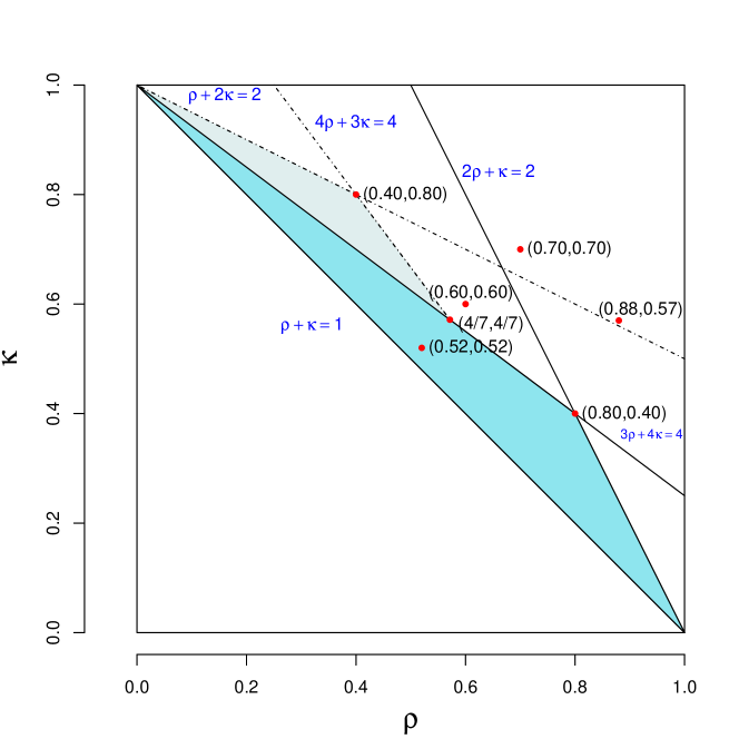
Figure 1: The large shaded triangle is the domain of interest $\mathcal{D}$ for Theorem 2. The smaller shaded triangle shows a region where the analogous update to $\boldsymbol{a}$ would have acceptable norm. The points marked are the ones we look at numerically, including $(0.88,0.57)$ which corresponds to the Stitch Fix data in Section 6.

Proof.

Without loss of generality we assume that $\epsilon<1$. We begin with (35). Let $M=M^{(2)}$. When $j\neq s$,

$$M_{js} =\frac{1}{N_{\text{\tiny$\bullet$}j}+\lambda_{B}}\sum_{r}\frac{Z_{rj}}{N_{r\text{\tiny$\bullet$}}+\lambda_{A}}(Z_{rs}-\bar{Z}_{\text{\tiny$\bullet$}s}),\quad\text{for}$$

$$\bar{Z}_{\text{\tiny$\bullet$}s} =\sum_{i}\frac{Z_{is}}{N_{i\text{\tiny$\bullet$}}+\lambda_{A}}\Bigm{/}{\sum_{i}\frac{1}{N_{i\text{\tiny$\bullet$}}+\lambda_{A}}}.$$

Although $|Z_{rs}-\bar{Z}_{\text{\tiny$\bullet$}s}|\leqslant 1$, replacing $Z_{rs}-\bar{Z}_{\text{\tiny$\bullet$}s}$ by one does not prove to be sharp enough for our purposes.

Every $N_{r\text{\tiny$\bullet$}}+\lambda_{A}\in S^{1-\rho}[1-\epsilon,\Upsilon+\epsilon]$ with probability tending to one and so

$$\frac{\bar{Z}_{\text{\tiny$\bullet$}s}}{N_{\text{\tiny$\bullet$}j}+\lambda_{B}}\sum_{r}\frac{Z_{rj}}{N_{r\text{\tiny$\bullet$}}+\lambda_{A}} \in\frac{\bar{Z}_{\text{\tiny$\bullet$}s}}{N_{\text{\tiny$\bullet$}j}+\lambda_{B}}\sum_{r}\frac{Z_{rj}}{[1-\epsilon,\Upsilon+\epsilon]S^{1-\rho}}$$

$$\subseteq[1-\epsilon,\Upsilon+\epsilon]^{-1}\bar{Z}_{\text{\tiny$\bullet$}s}S^{\rho-1}.$$

Similarly

$$\bar{Z}_{\text{\tiny$\bullet$}s} \in\frac{\sum_{i}Z_{is}[1-\epsilon,\Upsilon+\epsilon]^{-1}}{R[1-\epsilon,\Upsilon+\epsilon]^{-1}}\subseteq\frac{N_{\text{\tiny$\bullet$}s}}{R}[1-\epsilon,\Upsilon+\epsilon][1-\epsilon,\Upsilon+\epsilon]^{-1}$$

$$\subseteq S^{1-\rho-\kappa}[1-\epsilon,\Upsilon+\epsilon]^{2}[1-\epsilon,\Upsilon+\epsilon]^{-1}$$

and so

$$\frac{\bar{Z}_{\text{\tiny$\bullet$}s}}{N_{\text{\tiny$\bullet$}j}+\lambda_{B}}\sum_{r}\frac{Z_{rj}}{N_{r\text{\tiny$\bullet$}}+\lambda_{A}}\in S^{-\kappa}\frac{[1-\epsilon,\Upsilon+\epsilon]^{2}}{[1-\epsilon,\Upsilon+\epsilon]^{2}}\subseteq\frac{1}{C}\Bigl{[}\Bigl{(}\frac{1-\epsilon}{\Upsilon+\epsilon}\Bigr{)}^{2},\Bigl{(}\frac{\Upsilon+\epsilon}{1-\epsilon}\Bigr{)}^{2}\Bigr{]}.$$ (36)

Next using bounds on the co-observation counts,

$$\frac{1}{N_{\text{\tiny$\bullet$}j}+\lambda_{B}}\sum_{r}\frac{Z_{rj}Z_{rs}}{N_{r\text{\tiny$\bullet$}}+\lambda_{A}}\in\frac{S^{\rho+\kappa-2}(Z^{\mathsf{T}}Z)_{sj}}{[1-\epsilon,\Upsilon+\epsilon]^{2}}\subseteq\frac{1}{C}\frac{[1-\epsilon,\Upsilon^{2}+\epsilon]}{[1-\epsilon,\Upsilon+\epsilon]^{2}}.$$ (37)

Combining (36) and (37)

$$M_{js}\in \frac{1}{C}\Bigl{[}\frac{1-\epsilon}{(\Upsilon+\epsilon)^{2}}-\Bigl{(}\frac{\Upsilon+\epsilon}{1-\epsilon}\Bigr{)}^{2},\frac{\Upsilon^{2}+\epsilon}{1-\epsilon}-\Bigl{(}\frac{1-\epsilon}{\Upsilon+\epsilon}\Bigr{)}^{2}\Bigr{]}$$

For any $\epsilon^{\prime}>0$ we can choose $\epsilon$ small enough that

$$M_{js}\in C^{-1}[\Upsilon^{-2}-\Upsilon^{2}-\epsilon^{\prime},\Upsilon^{2}-\Upsilon^{-2}+{\epsilon^{\prime}}]$$

and then $|M_{js}|\leqslant(\Upsilon^{2}-\Upsilon^{-2}+\epsilon^{\prime})/C$.

Next, arguments like the preceding give $|M_{jj}|\leqslant(1-\epsilon^{\prime})^{-2}(\Upsilon+\epsilon^{\prime})S^{\rho-1}\to 0$. Then with probability tending to one,

$$\sum_{j}|M_{js}|\leqslant\Upsilon^{2}-\Upsilon^{-2}+2\epsilon^{\prime}.$$

This bound holds for all $s\in\{1,2,\dots,C\}$, establishing (35).

The proof of (34) is similar. The quantity $\bar{Z}_{\text{\tiny$\bullet$}s}$ is replaced by $(1/R)\sum_{i}Z_{is}/(N_{i\text{\tiny$\bullet$}}+\lambda_{A})$. ∎

It is interesting to find the largest $\Upsilon$ with $\Upsilon^{2}-\Upsilon^{-2}\leqslant 1$. It is $((1+5^{1/2})/2)^{1/2}\doteq 1.27$.

5 Convergence and computation

In this section we make some computations on synthetic data following the probability model from Section 4. First we study the norms of our update matrix $M^{(2)}$ which affects the number of iterations to convergence. In addition to $\|\cdot\|_{1}$ covered in Theorem 2 we also consider $\|\cdot\|_{2}$, $\|\cdot\|_{\infty}$ and $\lambda_{\max}(\cdot)$. Then we compare the cost to compute $\hat{\beta}_{\mathrm{GLS}}$ by our backfitting method with that of lmer (Bates et al.,, 2015).

The problem size is indexed by $S$. Indices $i$ go from $1$ to $R=\lceil S^{\rho}\rceil$ and indices $j$ go from $1$ to $C=\lceil S^{\kappa}\rceil$. Reasonable parameter values have $\rho,\kappa\in(0,1)$ with $\rho+\kappa>1$. Theorem 2 applies when $2\rho+\kappa<2$ and $3\rho+4\kappa<4$. Figure 1 depicts this triangular domain of interest $\mathcal{D}$. There is another triangle $\mathcal{D}^{\prime}$ where a corresponding update for $\boldsymbol{a}$ would satisfy the conditions of Theorem 2. Then $\mathcal{D}\cup\mathcal{D}^{\prime}$ is a non-convex polygon of five sides. Figure 1 also shows $\mathcal{D}^{\prime}\setminus\mathcal{D}$ as a second triangular region. For points $(\rho,\kappa)$ near the line $\rho+\kappa=1$, the matrix $Z$ will be mostly ones unless $S$ is very large. For points $(\rho,\kappa)$ near the upper corner $(1,1)$, the matrix $Z$ will be extremely sparse with each $N_{i\text{\tiny$\bullet$}}$ and $N_{\text{\tiny$\bullet$}j}$ having nearly a Poisson distribution with mean between $1$ and $\Upsilon$. The fraction of potential values that have been observed is $O(S^{1-\rho-\kappa})$.

Given $p_{ij}$, we generate our observation matrix via $Z_{ij}\stackrel{{\scriptstyle\mathrm{ind}}}{{\sim}}\mathrm{Bern}({p_{ij})}$. These probabilities are first generated via ${p_{ij}}=U_{ij}S^{1-\rho-\kappa}$ where $U_{ij}\stackrel{{\scriptstyle\mathrm{iid}}}{{\sim}}\mathbb{U}[1,\Upsilon]$ and $\Upsilon$ is the largest value for which $\Upsilon^{2}-\Upsilon^{-2}\leqslant 1$. For small $S$ and $\rho+\kappa$ near $1$ we can get some values ${p_{ij}>1}$ and in that case we take ${p_{ij}=1}$.

The following $(\rho,\kappa)$ combinations are of interest. First, $(4/5,2/5)$ is the closest vertex of the domain of interest to the point $(1,1)$. Second, $(2/5,4/5)$ is outside the domain of interest for the $\boldsymbol{b}$ but within the domain for the analogous $\boldsymbol{a}$ update. Third, among points with $\rho=\kappa$, the value $(4/7,4/7)$ is the farthest one from the origin that is in the domain of interest. We also look at some points on the $45$ degree line that are outside the domain of interest because the sufficient conditions in Theorem 2 might not be necessary.

In our matrix norm computations we took $\lambda_{A}=\lambda_{B}=0$. This completely removes shrinkage and will make it harder for the algorithm to converge than would be the case for the positive $\lambda_{A}$ and $\lambda_{B}$ that hold in real data. The values of $\lambda_{A}$ and $\lambda_{B}$ appear in expressions $N_{i\text{\tiny$\bullet$}}+\lambda_{A}$ and $N_{\text{\tiny$\bullet$}j}+\lambda_{B}$ where their contribution is asymptotically negligible, so conservatively setting them to zero will nonetheless be realistic for large data sets.

Figure 2: Norm $\|M^{(2)}\|_{1}$ of centered update matrix versus problem size $S$ for different $(\rho,\kappa)$.

We sample from the model multiple times at various values of $S$ and plot $\|M^{(2)}\|_{1}$ versus $S$ on a logarithmic scale. Figure 2 shows the results. We observe that $\|M^{(2)}\|_{1}$ is below $1$ and decreasing with $S$ for all the examples $(\rho,\kappa)\in\mathcal{D}$. This holds also for $(\rho,\kappa)=(0.60,0.60)\not\in\mathcal{D}$. We chose that point because it is on the convex hull of $\mathcal{D}\cup\mathcal{D}^{\prime}$.

The point $(\rho,\kappa)=(0.40,0.80)\not\in\mathcal{D}$. Figure 2 shows large values of $\|M^{(2)}\|_{1}$ for this case. Those values increase with $S$, but remain below $1$ in the range considered. This is a case where the update from $\boldsymbol{a}$ to $\boldsymbol{a}$ would have norm well below $1$ and decreasing with $S$, so backfitting would converge. We do not know whether $\|M^{(2)}\|_{1}>1$ will occur for larger $S$.

The point $(\rho,\kappa)=(0.70,0.70)$ is not in the domain $\mathcal{D}$ covered by Theorem 2 and we see that $\|M^{(2)}\|_{1}>1$ and generally increasing with $S$ as shown in Figure 3. This does not mean that backfitting must fail to converge. Here we find that $\|M^{(2)}\|_{2}<1$ and generally decreases as $S$ increases. This is a strong indication that the number of backfitting iterations required will not grow with $S$ for this $(\rho,\kappa)$ combination. We cannot tell whether $\|M^{(2)}\|_{2}$ will decrease to zero but that is what appears to happen.

We consistently find in our computations that $\lambda_{\max}(M^{(2)})\leqslant\|M^{(2)}\|_{2}\leqslant\|M^{(2)}\|_{1}$. The first of these inequalities must necessarily hold. For a symmetric matrix $M$ we know that $\lambda_{\max}(M)=\|M\|_{2}$ which is then necessarily no larger than $\|M\|_{1}$. Our update matrices are nearly symmetric but not perfectly so. We believe that explains why their $L_{2}$ norms are close to their spectral radius and also smaller than their $L_{1}$ norms. While the $L_{2}$ norms are empirically more favorable than the $L_{1}$ norms, they are not amenable to our theoretical treatment.

Figure 3: The left panel shows $\|M^{(2)}\|_{1}$ versus $S$. The right panel shows $\|M^{(2)}\|_{2}$ versus $S$ with a logarithmic vertical scale. Both have $(\rho,\kappa)=(0.7,0.7)$.

We believe that backfitting will have a spectral radius well below $1$ for more cases than we can as yet prove. In addition to the previous figures showing matrix norms as $S$ increases for certain special values of $(\rho,\kappa)$ we have computed contour maps of those norms over $(\rho,\kappa)\in[0,1]$ for $S=10{,}000$. See Figure 4.

To compare the computation times for algorithms we generated $Z_{ij}$ as above and also took $x_{ij}\stackrel{{\scriptstyle\mathrm{iid}}}{{\sim}}\mathcal{N}(0,I_{7})$ plus an intercept, making $p=8$ fixed effect parameters. Although backfitting can run with $\lambda_{A}=\lambda_{B}=0$, lmer cannot do so for numerical reasons. So we took $\sigma^{2}_{A}=\sigma^{2}_{B}=1$ and $\sigma^{2}_{E}=1$ corresponding to $\lambda_{A}=\lambda_{B}=1$. The cost per iteration does not depend on $Y_{ij}$ and hence not on $\beta$ either. We used $\beta=0$.

Figure 5 shows computation times for one single iteration when $(\rho,\kappa)=(0.52,0.52)$ and when $(\rho,\kappa)=(0.70,0.70)$. The time to do one iteration in lmer grows roughly like $N^{3/2}$ in the first case. For the second case, it appears to grow at the even faster rate of $N^{2.1}$. Solving a system of $S^{\kappa}\times S^{\kappa}$ equations would cost $S^{3\kappa}=S^{2.1}=O(N^{2.1})$, which explains the observed rate. This analysis would predict $O(N^{1.56})$ for $\rho=\kappa=0.52$ but that is only minimally different from $O(N^{3/2})$. These experiments were carried out in R on a computer with the macOS operating system, 16 GB of memory and an Intel i7 processor. Each backfitting iteration entails solving (17) along with the fixed effects.

The cost per iteration for backfitting follows closely to the $O(N)$ rate predicted by the theory. OLS only takes one iteration and it is also of $O(N)$ cost. In both of these cases $\|M^{(2)}\|_{2}$ is bounded away from one so the number of backfitting iterations does not grow with $S$. For $\rho=\kappa=0.52$, backfitting took $4$ iterations to converge for the smaller values of $S$ and $3$ iterations for the larger ones. For $\rho=\kappa=0.70$, backfitting took $6$ iterations for smaller $S$ and $4$ or $5$ iterations for larger $S$. In each case our convergence criterion was a relative change of $10^{-8}$ as described in Section 6.3. Further backfitting to compute BLUPs $\hat{\boldsymbol{a}}$ and $\hat{\boldsymbol{b}}$ given $\hat{\beta}_{\mathrm{GLS}}$ took at most $5$ iterations for $\rho=\kappa=0.52$ and at most $10$ iterations for $\rho=\kappa=0.7$. In the second example, lme4 did not reach convergence in our time window so we ran it for just $4$ iterations to measure its cost per iteration.

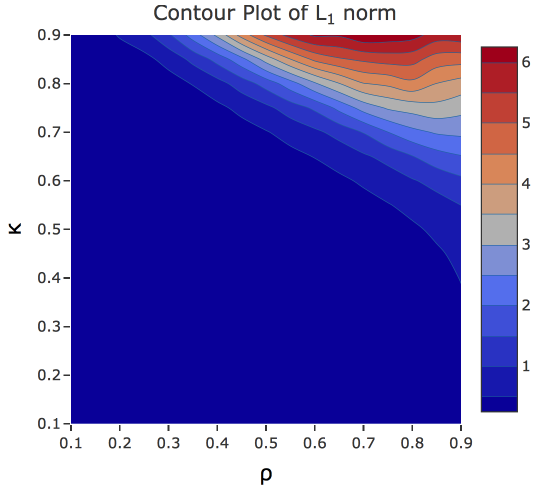
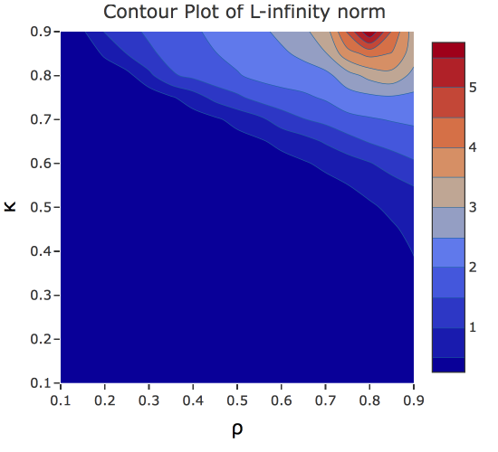
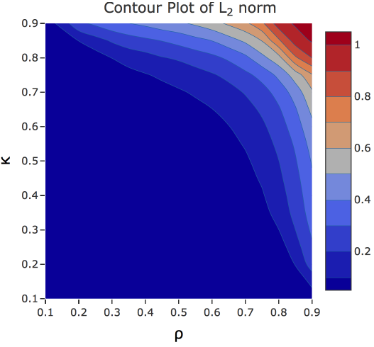
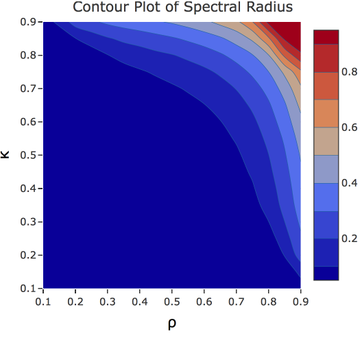
Figure 4: Numerically computed matrix norms for $M^{(2)}$ using $S=10{,}000$. The color code varies with the subfigures.

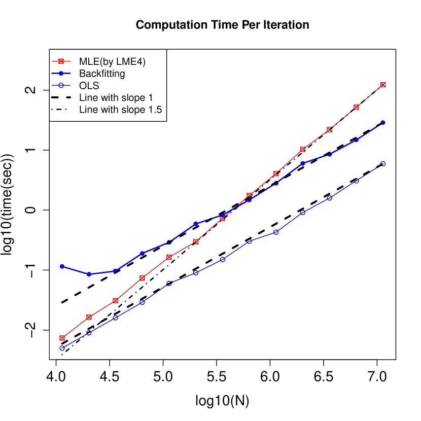
(a) $(\rho,\kappa)=(0.52,0.52)$

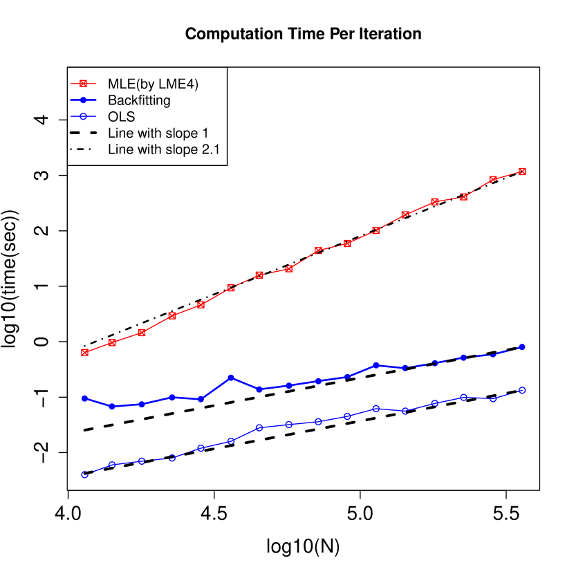
(b) $(\rho,\kappa)=(0.70,0.70)$

Figure 5: Time for one iteration versus the number of observations, $N$ at two points $(\rho,\kappa)$. The cost for lmer is roughly $O(N^{3/2})$ in the top panel and $O(N^{2.1})$ in the bottom panel. The costs for OLS and backfitting are $O(N)$.

6 Example: ratings from Stitch Fix

We illustrate backfitting for GLS on some data from Stitch Fix. Stitch Fix sells clothing. They mail their customers a sample of items. The customers may keep and purchase any of those items that they want, while returning the others. It is valuable to predict the extent to which a customer will like an item, not just whether they will purchase it. Stitch Fix has provided us with some of their client ratings data. It was anonymized, void of personally identifying information, and as a sample it does not reflect their total numbers of clients or items at the time they provided it. It is also from 2015. While it does not describe their current business, it is a valuable data set for illustrative purposes.

The sample sizes for this data are as follows. We received $N=5{,}000{,}000$ ratings by $R=762{,}752$ customers on $C=6{,}318$ items. These values of $R$ and $C$ correspond to the point $(0.88,0.57)$ in Figure 1. Thus $C/N\doteq 0.00126$ and $R/N\doteq 0.153$. The data are not dominated by a single row or column because $\max_{i}N_{i\text{\tiny$\bullet$}}/R\doteq 9\times 10^{-6}$ and $\max_{j}N_{\text{\tiny$\bullet$}j}/N\doteq 0.0143$. The data are sparse because $N/(RC)\doteq 0.001$.

6.1 An illustrative linear model

The response $Y_{ij}$ is a rating on a ten point scale of the satisfaction of customer $i$ with item $j$. The data come with features about the clients and items. In a business setting one would fit and compare possibly dozens of different regression models to understand the data. Our purpose here is to study large scale GLS and compare it to ordinary least squares (OLS) and so we use just one model, not necessarily one that we would have settled on. For that purpose we use the same model that was used in Gao and Owen, (2019). It is not chosen to make OLS look as bad as possible. Instead it is potentially the first model one might look at in a data analysis. For client $i$ and item $j$,

$$Y_{ij} =\beta_{0}+\beta_{1}\mathrm{match}_{ij}+\beta_{2}\mathbb{I}\{\mathrm{client\ edgy}\}_{i}+\beta_{3}\mathbb{I}\{\mathrm{item\ edgy}\}_{j}$$

$$\phantom{=}\,\,+\beta_{4}\mathbb{I}\{\mathrm{client\ edgy}\}_{i}*\mathbb{I}\{\mathrm{item\ edgy}\}_{j}+\beta_{5}\mathbb{I}\{\mathrm{client\ boho}\}_{i}$$

$$\phantom{=}\,\,+\beta_{6}\mathbb{I}\{\mathrm{item\ boho}\}_{j}+\beta_{7}\mathbb{I}\{\mathrm{client\ boho}\}_{i}*\mathbb{I}\{\mathrm{item\ boho}\}_{j}$$

$$\phantom{=}\,\,+\beta_{8}\mathrm{material}_{ij}+a_{i}+b_{j}+e_{ij}.$$

Here $\mathrm{material}_{ij}$ is a categorical variable that is implemented via indicator variables for each type of material other than the baseline. Following Gao and Owen, (2019), we chose ‘Polyester’, the most common material, as the baseline. Some customers and some items were given the adjective ‘edgy’ in the data set. Another adjective was ‘boho’, short for ‘Bohemian’. The variable match${}_{ij}\in[0,1]$ is an estimate of the probability that the customer keeps the item, made before the item was sent. The match score is a prediction from a baseline model and is not representative of all algorithms used at Stitch Fix. All told, the model has $p=30$ parameters.

6.2 Estimating the variance parameters

We use the method of moments method from Gao and Owen, (2019) to estimate $\theta^{\mathsf{T}}=(\sigma^{2}_{A},\sigma^{2}_{B},\sigma^{2}_{E})$ in $O(N)$ computation. That is in turn based on the method that Gao and Owen, (2017) use in the intercept only model where $Y_{ij}=\mu+a_{i}+b_{j}+e_{ij}$. For that model they set

$$U_{A} =\sum_{i}\sum_{j}Z_{ij}\Bigl{(}Y_{ij}-\frac{1}{N_{i\text{\tiny$\bullet$}}}\sum_{j^{\prime}}Z_{ij^{\prime}}Y_{ij^{\prime}}\Bigr{)}^{2},$$

$$U_{B} =\sum_{j}\sum_{i}Z_{ij}\Bigl{(}Y_{ij}-\frac{1}{N_{\text{\tiny$\bullet$}j}}\sum_{i^{\prime}}Z_{i^{\prime}j}Y_{i^{\prime}j}\Bigr{)}^{2},\quad\text{and}$$

$$U_{E} =N\sum_{ij}Z_{ij}\Bigl{(}Y_{ij}-\frac{1}{N}\sum_{i^{\prime}j^{\prime}}Z_{i^{\prime}j^{\prime}}Y_{i^{\prime}j^{\prime}}\Bigr{)}^{2}.$$

These are, respectively, sums of within row sums of squares, sums of within column sums of squares and a scaled overall sum of squares. Straightforward calculations show that

$$\mathbb{E}(U_{A}) =\bigl{(}\sigma^{2}_{B}+\sigma^{2}_{E}\bigr{)}(N-R),$$

$$\mathbb{E}(U_{B}) =\bigl{(}\sigma^{2}_{A}+\sigma^{2}_{E}\bigr{)}(N-C),\quad\text{and}$$

$$\mathbb{E}(U_{E}) =\sigma^{2}_{A}\Bigl{(}N^{2}-\sum_{i}N_{i\text{\tiny$\bullet$}}^{2}\Bigr{)}+\sigma^{2}_{B}\Bigl{(}N^{2}-\sum_{j}N_{\text{\tiny$\bullet$}j}^{2}\Bigr{)}+\sigma^{2}_{E}(N^{2}-N).$$

By matching moments, we can estimate $\theta$ by solving the $3\times 3$ linear system

$$\begin{pmatrix}0&N-R&N-R\\[1.07639pt] N-C&0&N-C\\[1.07639pt] N^{2}-\Sigma N_{i}^{2}&N^{2}-\Sigma N_{j}^{2}&N^{2}-N\end{pmatrix}\begin{pmatrix}\sigma^{2}_{A}\\[1.07639pt] \sigma^{2}_{B}\\[1.07639pt] \sigma^{2}_{E}\end{pmatrix}=\begin{pmatrix}U_{A}\\[1.07639pt] U_{B}\\[1.07639pt] U_{E}\end{pmatrix}$$

for $\theta$.

Following Gao and Owen, (2017) we note that $\eta_{ij}=Y_{ij}-x_{ij}^{\mathsf{T}}\beta=a_{i}+b_{j}+e_{ij}$ has the same parameter $\theta$ as $Y_{ij}$ have. We then take a consistent estimate of $\beta$, in this case $\hat{\beta}_{\mathrm{OLS}}$ that Gao and Owen, (2017) show is consistent for $\beta$, and define $\hat{\eta}_{ij}=Y_{ij}-x_{ij}^{\mathsf{T}}\hat{\beta}_{\mathrm{OLS}}$. We then estimate $\theta$ by the above method after replacing $Y_{ij}$ by $\hat{\eta}_{ij}$. For the Stitch Fix data we obtained $\hat{\sigma}_{A}^{2}=1.14$ (customers), $\hat{\sigma}^{2}_{B}=0.11$ (items) and $\hat{\sigma}^{2}_{E}=4.47$.

6.3 Computing $\hat{\beta}_{\mathrm{GLS}}$

The estimated coefficients $\hat{\beta}_{\mathrm{GLS}}$ and their standard errors are presented in a table in the appendix. Open-source R code at https://github.com/G28Sw/backfit_code does these computations. Here is a concise description of the algorithm we used:

1. Compute $\hat{\beta}_{\mathrm{OLS}}$ via (2).

2. Get residuals $\hat{\eta}_{ij}=Y_{ij}-x_{ij}^{\mathsf{T}}\hat{\beta}_{\mathrm{OLS}}$.

3. Compute $\hat{\sigma}^{2}_{A}$, $\hat{\sigma}^{2}_{B}$ and $\hat{\sigma}^{2}_{E}$ by the method of moments on $\hat{\eta}_{ij}$.

4. Compute $\widetilde{\mathcal{X}}=(I_{N}-\widetilde{\mathcal{S}}_{G})\mathcal{X}$ using doubly centered backfitting $M^{(3)}$.

5. Compute $\hat{\beta}_{\mathrm{GLS}}$ by (28).

6. If we want BLUPs $\hat{\boldsymbol{a}}$ and $\hat{\boldsymbol{b}}$ backfit $\mathcal{Y}-\mathcal{X}\hat{\beta}_{\mathrm{GLS}}$ to get them.

7. Compute $\widehat{\mathrm{cov}}(\hat{\beta}_{\mathrm{GLS}})$ by plugging $\hat{\sigma}^{2}_{A}$, $\hat{\sigma}^{2}_{B}$ and $\hat{\sigma}^{2}_{E}$ into $\mathcal{V}$ at (28).

Stage $k$ of backfitting provides $(\tilde{\mathcal{S}}_{G}\mathcal{X})^{(k)}$. We iterate until

$$\frac{\|(\tilde{\mathcal{S}}_{G}\mathcal{X})^{(k+1)}-(\tilde{\mathcal{S}}_{G}\mathcal{X})^{(k)}\|^{2}_{F}}{\|(\tilde{\mathcal{S}}_{G}\mathcal{X})^{(k)}\|^{2}_{F}}<\epsilon$$

where $\|\cdot\|_{F}$ is the Frobenius norm (root mean square of all elements). Our numerical results use $\epsilon=10^{-8}$.

When we want $\widehat{\mathrm{cov}}(\hat{\beta}_{\mathrm{GLS}})$ then we need to use a backfitting strategy with a symmetric smoother $\tilde{\mathcal{S}}_{G}$. This holds for $M^{(0)}$, $M^{(2)}$ and $M^{(3)}$ but not $M^{(1)}$. After computing $\hat{\beta}_{\mathrm{GLS}}$ one can return to step 2, form new residuals $\hat{\eta}_{ij}=Y_{ij}-x_{ij}^{\mathsf{T}}\hat{\beta}_{\mathrm{GLS}}$ and continue through steps 3–7. We have seen small differences from doing this.

6.4 Quantifying inefficiency and naivete of OLS

In the introduction we mentioned two serious problems with the use of OLS on crossed random effects data. The first is that OLS is naive about correlations in the data and this can lead it to severely underestimate the variance of $\hat{\beta}$. The second is that OLS is inefficient compared to GLS by the Gauss-Markov theorem. Let $\hat{\beta}_{\mathrm{OLS}}$ and $\hat{\beta}_{\mathrm{GLS}}$ be the OLS and GLS estimates of $\beta$, respectively. We can compute their corresponding variance estimates $\widehat{\mathrm{cov}}_{\mathrm{OLS}}(\hat{\beta}_{\mathrm{OLS}})$ and $\widehat{\mathrm{cov}}_{\mathrm{GLS}}(\hat{\beta}_{\mathrm{GLS}})$. We can also find $\widehat{\mathrm{cov}}_{\mathrm{GLS}}(\hat{\beta}_{\mathrm{OLS}})$, the variance under our GLS model of the linear combination of $Y_{ij}$ values that OLS uses. This section explore them graphically.

We can quantify the naivete of OLS via the ratios $\widehat{\mathrm{cov}}_{\mathrm{GLS}}(\hat{\beta}_{\mathrm{OLS},j})/\widehat{\mathrm{cov}}_{\mathrm{OLS}}(\hat{\beta}_{\mathrm{OLS},j})$ for $j=1,\dots,p$. Figure 6 plots these values. They range from $1.75$ to $345.28$ and can be interpreted as factors by which OLS naively overestimates its sample size. The largest and second largest ratios are for material indicators corresponding to ‘Modal’ and ‘Tencel’, respectively. These appear to be two names for the same product with Tencel being a trademarked name for Modal fibers (made from wood). We can also identify the linear combination of $\hat{\beta}_{\mathrm{OLS}}$ for which $\mathrm{OLS}$ is most naive. We maximize the ratio $x^{\mathsf{T}}\widehat{\mathrm{cov}}_{\mathrm{GLS}}(\hat{\beta}_{\mathrm{OLS}})x/x^{\mathsf{T}}\widehat{\mathrm{cov}}_{\mathrm{OLS}}(\hat{\beta}_{\mathrm{OLS}})x$ over $x\neq 0$. The resulting maximal ratio is the largest eigenvalue of

$$\widehat{\mathrm{cov}}_{\mathrm{OLS}}(\hat{\beta}_{\mathrm{OLS}})^{-1}\widehat{\mathrm{cov}}_{\mathrm{GLS}}(\hat{\beta}_{\mathrm{OLS}})$$

and it is about $361$ for the Stitch Fix data.

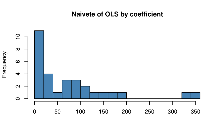
Figure 6: OLS naivete $\widehat{\mathrm{cov}}_{\mathrm{GLS}}(\hat{\beta}_{\mathrm{OLS},j})/\widehat{\mathrm{cov}}_{\mathrm{OLS}}(\hat{\beta}_{\mathrm{OLS},j})$ for coefficients $\beta_{j}$ in the Stitch Fix data.

We can quantify the inefficiency of OLS via the ratio $\widehat{\mathrm{cov}}_{\mathrm{GLS}}(\hat{\beta}_{\mathrm{OLS},j})/\widehat{\mathrm{cov}}_{\mathrm{GLS}}(\hat{\beta}_{\mathrm{GLS},j})$ for $j=1,\dots,p$. Figure 7 plots these values. They range from just over $1$ to $50.6$ and can be interpreted as factors by which using OLS reduces the effective sample size. There is a clear outlier: the coefficient of the match variable is very inefficiently estimated by OLS. The second largest inefficiency factor is for the intercept term. The most inefficient linear combination of $\hat{\beta}$ reaches a variance ratio of $52.6$, only slightly more inefficient than the match coefficient alone.

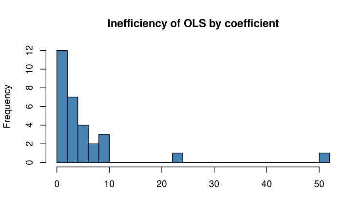
Figure 7: OLS inefficiency $\widehat{\mathrm{cov}}_{\mathrm{GLS}}(\hat{\beta}_{\mathrm{OLS},j})/\widehat{\mathrm{cov}}_{\mathrm{GLS}}(\hat{\beta}_{\mathrm{GLS},j})$ for coefficients $\beta_{j}$ in the Stitch Fix data.

The variables for which OLS is more naive tend to also be the variables for which it is most inefficient. Figure 8 plots these quantities against each other for the $30$ coefficients in our model.

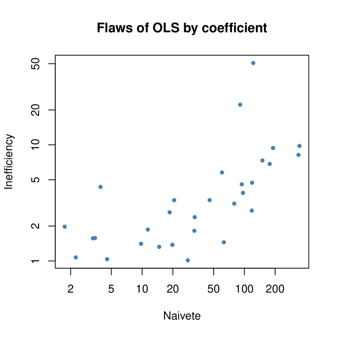
Figure 8: Inefficiency vs naivete for OLS coefficients in the Stitch Fix data.

6.5 Convergence speed of backfitting

The Stitch Fix data have row and column sample sizes that are much more uneven than our sampling model for $Z$ allows. Accordingly we cannot rely on Theorem 2 to show that backfitting must converge rapidly for it.

The sufficient conditions in that theorem may not be necessary and we can compute our norms and the spectral radius on the update matrices for the Stitch Fix data using some sparse matrix computations. Here $Z\in\{0,1\}^{762,752\times 6318}$, so $M^{(k)}\in\mathbb{R}^{6318\times 6318}$ for $k\in\{0,1,2,3\}$. The results are

$$\begin{pmatrix}\|M^{(0)}\|_{1}\ &\ \|M^{(0)}\|_{2}\ &\ |\lambda_{\max}(M^{(0)})|\\[1.07639pt] \|M^{(1)}\|_{1}\ &\ \|M^{(1)}\|_{2}\ &\ |\lambda_{\max}(M^{(1)})|\\[1.07639pt] \|M^{(2)}\|_{1}\ &\ \|M^{(2)}\|_{2}\ &\ |\lambda_{\max}(M^{(2)})|\\[1.07639pt] \|M^{(3)}\|_{1}\ &\ \|M^{(3)}\|_{2}\ &\ |\lambda_{\max}(M^{(3)})|\end{pmatrix}=\begin{pmatrix}31.9525\ &\ 1.4051\ &\ 0.64027\\[3.22916pt] 11.2191\ &\ 0.4512\ &\ 0.33386\\[3.22916pt] \phantom{0}8.9178\ &\ 0.4541\ &\ 0.33407\\[3.22916pt] \phantom{0}9.2143\ &\ 0.4546&\ 0.33377\\ \end{pmatrix}.$$

All the updates have spectral radius comfortably below one. The centered updates have $L_{2}$ norm below one but the uncentered update does not. Their $L_{2}$ norms are somewhat larger than their spectral radii because those matrices are not quite symmetric. The two largest eigenvalue moduli for $M^{(0)}$ are $0.6403$ and $0.3337$ and the centered updates have spectral radii close to the second largest eigenvalue of $M^{(0)}$. This is consistent with an intuitive explanation that the space spanned by a column of $N$ ones that is common to the columns spaces of $\mathcal{Z}_{A}$ and $\mathcal{Z}_{B}$ is the biggest impediment to $M^{(0)}$ and that all three centering strategies essentially remove it. The best spectral radius is for $M^{(3)}$, which employs two principled centerings, although in this data set it made little difference. Our backfitting algorithm took $8$ iterations when applied to $\mathcal{X}$ and $12$ more to compute the BLUPs. We used a convergence threshold of $10^{-8}.$

7 Discussion

We have shown that the cost of our backfitting algorithm is $O(N)$ under strict conditions that are nonetheless much more general than having $N_{i\text{\tiny$\bullet$}}=N/C$ for all $i=1,\dots,R$ and $N_{\text{\tiny$\bullet$}j}=N/R$ for all $j=1,\dots,C$ as in Papaspiliopoulos et al., (2020). As in their setting, the backfitting algorithm scales empirically to much more general problems than those for which rapid convergence can be proved. Our contour map of the spectral radius of the update matrix $M$ shows that this norm is well below $1$ over many more $(\rho,\kappa)$ pairs that our theorem covers. The difficulty in extending our approach to those settings is that the spectral radius is a much more complicated function of the observation matrix $Z$ than the $L_{1}$ norm is.

Theorem 4 of Papaspiliopoulos et al., (2020) has the rate of convergence for their collapsed Gibbs sampler for balanced data. It involves an auxilliary convergence rate $\rho_{\mathrm{aux}}$ defined as follows. Consider the Gibbs sampler on $(i,j)$ pairs where given $i$ a random $j$ is chosen with probability $Z_{ij}/N_{i\text{\tiny$\bullet$}}$ and given $j$ a random $i$ is chosen with probability $Z_{ij}/N_{\text{\tiny$\bullet$}j}$. That Markov chain has invariant distribution $Z_{ij}/N$ on $(i,j)$ pairs and $\rho_{\mathrm{aux}}$ is the rate at which the chain converges. In our notation

$$\rho_{\mathrm{PRZ}}=\frac{N\sigma^{2}_{A}}{N\sigma^{2}_{A}+R\sigma^{2}_{E}}\times\frac{N\sigma^{2}_{B}}{N\sigma^{2}_{B}+C\sigma^{2}_{E}}\times\rho_{\mathrm{aux}}.$$

In sparse data $\rho_{\mathrm{PRZ}}\approx\rho_{\mathrm{aux}}$ and under our asymptotic setting $|\rho_{\mathrm{aux}}-\rho_{\mathrm{PRZ}}|\to 0$. Papaspiliopoulos et al., (2020) remark that $\rho_{\mathrm{aux}}$ tends to decrease as the amount of data increases. When it does, then their algorithm takes $O(1)$ iterations and costs $O(N)$. They explain that $\rho_{\mathrm{aux}}$ should decrease as the data set grows because the auxiliary process then gets greater connectivity. That connectivity increases for bounded $R$ and $C$ with increasing $N$ and from their notation, allowing multiple observations per $(i,j)$ pair it seems like they have this sort of infill asymptote in mind. For sparse data from electronic commerce we think that an asymptote like the one we study where $R$, $C$ and $N$ all grow is a better description. It would be interesting to see how $\rho_{\mathrm{aux}}$ develops under such a model.

In Section 5.3 Papaspiliopoulos et al., (2020) state that the convergence rate of the collapsed Gibbs sampler is $O(1)$ regardless of the asymptotic regime. That section is about a more stringent ‘balanced cells’ condition where every $(i,j)$ combination is observed the same number of times, so it does not describe the ‘balanced levels’ setting where $N_{i\text{\tiny$\bullet$}}=N/R$ and $N_{\text{\tiny$\bullet$}j}=N/C$. Indeed they provide a counterexample in which there are two disjoint communities of users and two disjoint sets of items and each user in the first community has rated every item in the first item set (and no others) while each user in the second community has rated every item in the second item set (and no others). That configuration leads to an unbounded mixing time for collapsed Gibbs. It is also one where backfitting takes an increasing number of iterations as the sample size grows.

There are interesting parallels between methods to sample a high dimensional Gaussian distribution with covariance matrix $\Sigma$ and iterative solvers for the system $\Sigma\boldsymbol{x}=\boldsymbol{b}$. See Goodman and Sokal, (1989) and Roberts and Sahu, (1997) for more on how the convergence rates for these two problems coincide. We found that backfitting with one or both updates centered worked much better than uncentered backfitting. Papaspiliopoulos et al., (2020) used a collapsed sampler that analytically integrated out the global mean of their model in each update of a block of random effects.

Our approach treats $\sigma^{2}_{A}$, $\sigma^{2}_{B}$ and $\sigma^{2}_{E}$ as nuisance parameters. We plug in a consistent method of moments based estimator of them in order to focus on the backfitting iterations. In Bayesian computations, maximum a posteriori estimators of variance components under non-informative priors can be problematic for hierarchical models Gelman, (2006), and so perhaps maximum likelihood estimation of these variance components would also have been challenging.

Whether one prefers a GLS estimate or a Bayesian one depends on context and goals. We believe that there is a strong computational advantage to GLS for large data sets. The cost of one backfitting iteration is comparable to the cost to generate one more sample in the MCMC. We may well find that only a dozen or so iterations are required for convergence of the GLS. A Bayesian analysis requires a much larger number of draws from the posterior distribution than that. For instance, Gelman and Shirley, (2011) recommend an effective sample size of about $100$ posterior draws, with autocorrelations requiring a larger actual sample size. Vats et al., (2019) advocate even greater effective sample sizes.

It is usually reasonable to assume that there is a selection bias underlying which data points are observed. Accounting for any such selection bias must necessarily involve using information or assumptions from outside the data set at hand. We expect that any approach to take proper account of informative missingness must also make use of solutions to GLS perhaps after reweighting the observations. Before one develops any such methods, it is necessary to first be able to solve GLS without regard to missingness.

Many of the problems in electronic commerce involve categorical outcomes, especially binary ones, such as whether an item was purchased or not. Generalized linear mixed models are then appropriate ways to handle crossed random effects, and we expect that the progress made here will be useful for those problems.

8 Appendix

Table 1 shows results of $\mathrm{OLS}$ and $\mathrm{GLS}$ regression for the Stitch Fix data in Section 6. OLS is estimated to be naive when $\widehat{\mathrm{SE}}_{\mathrm{OLS}}(\hat{\beta}_{\mathrm{OLS}})<\widehat{\mathrm{SE}}_{\mathrm{GLS}}(\hat{\beta}_{\mathrm{OLS}})$ and inefficient when $\widehat{\mathrm{SE}}_{\mathrm{OLS}}(\hat{\beta}_{\mathrm{OLS}})>\widehat{\mathrm{SE}}_{\mathrm{GLS}}(\hat{\beta}_{\mathrm{GLS}})$. Estimates that are more than double their corresponding standard error get an asterisk.

Table 1: Stitch Fix Regression Results

	$\hat{\beta}_{\mathrm{OLS}}$	$\widehat{\mathrm{SE}}_{\mathrm{OLS}}(\hat{\beta}_{\mathrm{OLS}})$	$\widehat{\mathrm{SE}}_{\mathrm{GLS}}(\hat{\beta}_{\mathrm{OLS}})$	$\hat{\beta}_{\mathrm{GLS}}$	$\widehat{\mathrm{SE}}_{\mathrm{GLS}}(\hat{\beta}_{\mathrm{GLS}})$
Intercept	$4.635^{*}$	$0.005397$	$0.05148$	$5.103^{*}$	$0.01092$
Match	$5.048^{*}$	$0.01174$	$0.1297$	$3.442^{*}$	$0.01823$
$\mathbb{I}\{\text{ client edgy }\}$	$0.001020$	$0.002443$	$0.004444$	$0.003041$	$0.003550$
$\mathbb{I}\{\text{ item edgy }\}$	$-0.3358^{*}$	$0.004253$	$0.03307$	$-0.3515^{*}$	$0.01375$
$\mathbb{I}\{\text{ client edgy }\}$
$*\mathbb{I}\{\text{ item edgy }\}$	$0.3925^{*}$	$0.006229$	$0.01233$	$0.3793^{*}$	$0.005916$
$\mathbb{I}\{\text{ client boho }\}$	$0.1386^{*}$	$0.002264$	$0.004211$	$0.1296^{*}$	$0.003356$
$\mathbb{I}\{\text{ item boho }\}$	$-0.5499^{*}$	$0.005981$	$0.02713$	$-0.6266^{*}$	$0.01485$
$\mathbb{I}\{\text{ client boho }\}$
$*\mathbb{I}\{\text{ item boho }\}$	$0.3822^{*}$	$0.007566$	$0.01001$	$0.3763^{*}$	$0.007123$
Acrylic	$-0.06482^{*}$	$0.003778$	$0.03371$	$-0.005360$	$0.01909$
Angora	$-0.01262$	$0.007848$	$0.08530$	$0.07486$	$0.05177$
Bamboo	$-0.04593$	$0.06215$	$0.2096$	$0.03251$	$0.1535$
Cashmere	$-0.1955^{*}$	$0.02484$	$0.1414$	$0.008930$	$0.1048$
Cotton	$0.1752^{*}$	$0.003172$	$0.04220$	$0.1033^{*}$	$0.01612$
Cupro	$0.5979^{*}$	$0.3016$	$0.4519$	$0.2089$	$0.4363$
Faux Fur	$0.2759^{*}$	$0.02008$	$0.07694$	$0.2749^{*}$	$0.06691$
Fur	$-0.2021^{*}$	$0.03121$	$0.1388$	$-0.07924$	$0.1182$
Leather	$0.2677^{*}$	$0.02482$	$0.07759$	$0.1674^{*}$	$0.06545$
Linen	$-0.3844^{*}$	$0.05632$	$0.2429$	$-0.08658$	$0.1499$
Modal	$0.002587$	$0.009775$	$0.1816$	$0.1388^{*}$	$0.05804$
Nylon	$0.03349^{*}$	$0.01552$	$0.08878$	$0.08174$	$0.05751$
Patent Leather	$-0.2359$	$0.1800$	$0.3838$	$-0.3764$	$0.3771$
Pleather	$0.4163^{*}$	$0.008916$	$0.08774$	$0.3292^{*}$	$0.04468$
PU	$0.4160^{*}$	$0.008225$	$0.07989$	$0.4579^{*}$	$0.03737$
PVC	$0.6574^{*}$	$0.06545$	$0.3462$	$0.9688^{*}$	$0.3441$
Rayon	$-0.01109^{*}$	$0.002951$	$0.04074$	$0.05155^{*}$	$0.01329$
Silk	$-0.1422^{*}$	$0.01317$	$0.08907$	$-0.1828^{*}$	$0.04871$
Spandex	$-0.3916^{*}$	$0.00931$	$0.1373$	$0.4140^{*}$	$0.1141$
Tencel	$0.4966^{*}$	$0.01729$	$0.1712$	$0.1234^{*}$	$0.05982$
Viscose	$0.04066^{*}$	$0.006953$	$0.08519$	$-0.02259$	$0.03145$
Wool	$-0.06021^{*}$	$0.006611$	$0.07211$	$-0.05883$	$0.03319$

References

- Bates et al., (2015) Bates, D., Mächler, M., Bolker, B., and Walker, S. (2015). Fitting linear mixed-effects models using lme4. Journal of Statistical Software, 67(1):1–48.
- Buja et al., (1989) Buja, A., Hastie, T., and Tibshirani, R. (1989). Linear smoothers and additive models (with discussion). The Annals of Statistics, pages 453–510.
- Cameron et al., (2011) Cameron, A. C., Gelbach, J. B., and Miller, D. L. (2011). Robust inference with multiway clustering. Journal of Business & Economic Statistics, 29(2):238–249.
- Gao, (2017) Gao, K. (2017). Scalable Estimation and Inference for Massive Linear Mixed Models with Crossed Random Effects. PhD thesis, Stanford University.
- Gao and Owen, (2017) Gao, K. and Owen, A. B. (2017). Efficient moment calculations for variance components in large unbalanced crossed random effects models. Electronic Journal of Statistics, 11(1):1235–1296.
- Gao and Owen, (2019) Gao, K. and Owen, A. B. (2019). Estimation and inference for very large linear mixed effects models. Statistica Sinica. To appear.
- Gelman, (2006) Gelman, A. (2006). Prior distributions for variance parameters in hierarchical models (comment on article by Browne and Draper). Bayesian analysis, 1(3):515–534.
- Gelman and Hill, (2006) Gelman, A. and Hill, J. (2006). Data analysis using regression and multilevel/hierarchical models. Cambridge University Press, Cambridge.
- Gelman and Shirley, (2011) Gelman, A. and Shirley, K. (2011). Inference from simulations and monitoring convergence. In Brooks, S., Gelman, A., Jones, G., and Meng, X.-L., editors, Handbook of Markov chain Monte Carlo, volume 6, pages 163–174. CRC Press Boca Raton, FL.
- Goodman and Sokal, (1989) Goodman, J. and Sokal, A. D. (1989). Multigrid Monte Carlo method. Conceptual foundations. Physical Review D, 40(6):2035–2071.
- Hastie and Tibshirani, (1990) Hastie, T. and Tibshirani, R. J. (1990). Generalized Additive Models. Chapman and Hall, Boca Raton, FL.
- Owen, (2007) Owen, A. B. (2007). The pigeonhole bootstrap. The Annals of Applied Statistics, 1(2):386–411.