SSIDS: Semi-Supervised Intrusion Detection System by Extending the Logical Analysis of Data

Abstract

Prevention of cyber attacks on the critical network resources has become an important issue as the traditional Intrusion Detection Systems (IDSs) are no longer effective due to the high volume of network traffic and the deceptive patterns of network usage employed by the attackers. Lack of sufficient amount of labeled observations for the training of IDSs makes the semi-supervised IDSs a preferred choice. We propose a semi-supervised IDS by extending a data analysis technique known as Logical Analysis of Data, or LAD in short, which was proposed as a supervised learning approach. LAD uses partially defined Boolean functions (pdBf) and their extensions to find the positive and the negative patterns from the past observations for classification of future observations. We extend the LAD to make it semi-supervised to design an IDS. The proposed SSIDS consists of two phases: offline and online. The offline phase builds the classifier by identifying the behavior patterns of normal and abnormal network usage. Later, these patterns are transformed into rules for classification and the rules are used during the online phase for the detection of abnormal network behaviors. The performance of the proposed SSIDS is far better than the existing semi-supervised IDSs and comparable with the supervised IDSs as evident from the experimental results.

Keywords:Intrusion Detection System, Logical Analysis of Data, Semi-Supervised Classification.

I Introduction

The Internet has evolved into a platform to deliver services from a platform to disseminate information. Consequently, misuse and policy violations by the attackers are routine affairs nowadays. Denning [11] introduced the concept of detecting the cyber threats by constant monitoring of network audit trails using Intrusion Detection System (IDS) to discover abnormal patterns or signatures of network or system usage. Recent advancements in IDS are related to the use of machine learning and soft computing techniques that have reduced the high false positive rates which were observed in the earlier generations of IDSs [15] [19]. The statistical models in the data mining techniques provide excellent intrusion detection capability to the designers of the existing IDSs which have increased their popularity. However, the inherent complications of IDSs such as competence, accuracy, and usability parameters make them unsuitable for deployment in a live system having high traffic volume. Further, the learning process of IDSs requires a large amount of training data which may not be always available, and it also requires a lot of computing power and time. Studies have revealed that it is difficult to handle high-speed network traffic by the existing IDSs due to their complex decision-making process. Attackers can take advantage of this shortcoming to hide their exploits and can overload an IDS using extraneous information while they are executing an attack. Therefore, building an efficient intrusion detection is vital for the security of the network system to prevent an attack in the shortest possible time.

A traditional IDS may discover network threats by matching current network behavior patterns with that of known attacks. The underlying assumption is that the behavior pattern in each attack is inherently different compared to the normal activity. Thus, only with the knowledge of normal behavior patterns, it may be possible to detect a new attack. However, the automatic generation of these patterns (or rules) is a challenging task, and most of the existing techniques require human intervention during pattern generation. Moreover, the lack of exhaustive prior knowledge (or labeled data) regarding the attacks makes this problem more challenging. It is advantageous for any IDS to consider unlabeled examples along with the available (may be small in number) labeled examples of the target class. This strategy helps in improving the accuracy of the IDSs against the new attacks. An IDS which can use both labeled and unlabeled examples is known as a semi-supervised IDS. Another important aspect of any intrusion detection system is the time required to detect abnormal activity. Detection in real time or near real time is preferred as it can prevent substantial damage to the resources. Thus, the primary objective of this work is to develop a semi-supervised intrusion detection system for near real-time detection of cyber threats.

Numerous security breaches of computer networks have encouraged researchers and practitioners to design several Intrusion Detection Systems. For a comprehensive review, we refer to [16]. Researchers have adopted various approaches to design IDSs, and a majority of them modeled the design problem as a classification problem. In [3], a feature selection method is used with a standard classifier like SVM as the conventional classifiers perform poorly due to the presence of redundant or irrelevant features. Authors of [20] also adopted a similar approach. Most of these designs share one common disadvantage, i.e., they follow a supervised learning approach. Recently, a new semi-supervised IDS has been proposed in [4], and it outperforms the existing semi-supervised IDSs, but it suffers from the low accuracy of detection.

It is essential to understand the behavior patterns of the known attacks, as well as the behaviors of normal activity to discover and prevent the attacks. Generation of patterns or signatures to model the normal as well as the abnormal activities is a tedious process, and it can be automatized using the application of LAD. Peter L. Hammer introduced the concept of logical analysis of data (or LAD) in the year $1986$ [12] and subsequently developed it as a technique to find the useful rules and patterns from the past observations to classify new observations [6, 9]. Patterns (or rules) can provide a very efficient way to solve various problems in different application areas, e.g., classification, development of rule-based decision support system, feature selection, medical diagnosis, network traffic analysis, etc. The initial versions of LAD [1, 9, 12] were designed to work with the binary data having either of the two labels, i.e., positive or negative. Thus, the data or observations were part of a two-class system. A specific goal of LAD is to learn the logical patterns which set apart observations of a class from the rest of the classes.

LAD has been used to analyze problems involving medical data. A typical dataset consists of two disjoint sets $\Omega^{+},\Omega^{-}$ which represent a set of observations consisting of positive and negative examples, respectively. Here, each observation is a vector consisting of different attribute values. In the domain of medical data analysis, each vector represents the medical record of a patient, and the patients in $\Omega^{+}$ have a specific medical condition. On the other hand, $\Omega^{-}$ represents the medical records of the patients who do not have that condition. Subsequently, if a new vector / patient is given, one has to decide whether the new vector belongs to $\Omega^{+}$ or $\Omega^{-}$, i.e., one has to determine whether the patient has the particular medical condition or not. Thus, in this example, the medical diagnosis problem can be interpreted as a two-class classification problem. The central theme of LAD is the selection of such patterns (or rules) which can collectively classify all the known observations. LAD stands out in comparison with other classification methods since a pattern can explain the classification outcome to human experts using formal reasoning.

Conventional LAD requires labeled examples for the pattern or rule generation. However, there exist several application domains (e.g., intrusion detection system, fraud detection, document clustering, etc.) where the existence of labeled examples are rare or insufficient. To harness the strength of LAD in these application domains, one needs to extend LAD for unsupervised and semi-supervised pattern generation [7]. Here, we introduce a preprocessing methodology using which we can extend the LAD in such a manner that it can use unlabeled observations along with the labeled observations for pattern generation. Consequently, it acts like a semi-supervised learning approach. The central theme is to use the classical LAD to generate initial positive and negative patterns from the available labeled observations. Once the patterns are available, we measure the closeness of the unlabeled observations with the initial positive or negative patterns using balance score. The observations with high positive balance score are labeled as the positive observations and the observations having high negative balance score are labeled as the negative examples. Once labels are generated, the standard LAD can be used as it is. We have used this approach successfully in the design of a new semi-supervised and lightweight Intrusion Detection System (IDS) which outperforms the existing methods in terms of accuracy and requirement of computational power.

Creation of signatures or patterns to model the normal as well as the abnormal network activities can be accomplished using the semi-supervised LAD (or S-LAD in short), and in this effort, we have used S-LAD to design a semi-supervised IDS. Here, S-LAD is used to generate the patterns which can differentiate the normal activities from the malicious activities, and these patterns are later converted to rules for the classification of unknown network behavior(s). The proposed SSIDS has two phases, the offline phase is used to design a rule-based classifier. This phase uses historical observations, both labeled and unlabeled, to find the patterns or rules of classification, and require a significant amount of processing power. Once the classification rules are generated, the online phase uses those rules to classify any new observation. The online phase requires much less processing power than the offline phase, and it can detect threats in near real-time. The accuracy of proposed semi-supervised IDS is much better than any state-of-the-art semi-supervised IDS and comparable with the supervised IDSs.

The main contributions of the proposed paper are: (1) a new implementation of LAD having extensively modified pattern generation algorithm; (2) a new strategy to extend LAD that is suitable for the design of semi-supervised classifiers; (3) a LAD-based design of a lightweight semi-supervised intrusion detection system that outperforms any existing semi-supervised IDSs.

The rest of the paper is organized as follows. Next section gives a brief description of our modified implementation of LAD and Section III describes the proposed method to extend LAD to the semi-supervised LAD. Details of the proposed SSIDS is available in the Section IV. Performance evaluation and comparative results are available in the Section V and we conclude the paper in the Section VI.

II Proposed Implementation of LAD

LAD is a data analysis technique which is inspired by the combinatorial optimization methods. As pointed out earlier, the initial version of LAD was designed to work with the binary data only. Let us first briefly describe the basic steps of LAD when it is applied to the binary data. An observation having $n$ attributes may be represented as a binary vector of length $n+1$ as the last bit (a.k.a. the class label) indicates whether it is a member of $\Omega^{+}$ or $\Omega^{-}$. Thus, the set of binary observations $\Omega$ ($=\Omega^{+}\cup\Omega^{-}\subseteq\{0,1\}^{n}$) can be represented by a partially defined Boolean function (pdBf in short) $\phi$, indicating a mapping of $\Omega\rightarrow\{0,1\}$. The goal of LAD is to find an extension $f$ of the pdBf $\phi$ which can classify all the unknown vectors in the sample space. However, this goal is clearly unachievable and we try to find an approximate extension $f^{\prime}$ of $f$. $f^{\prime}$ should approximate $f$ as closely as possible based on the several optimality criteria. Normally, the extension is represented in a disjunctive normal form (DNF). In brief, the LAD involves following steps [1].

1. Binarization of Observations. We have used a slightly modified implementation of binarization here.

2. Elimination of Redundancy (or Support Sets Generation).

3. Pattern Generation. Our extensively modified pattern generation algorithm makes the ’Theory Formation’ step redundant.

4. Theory Formation. We have omitted this step.

5. Classifier Design and Validation.

There are many application domains from the finance to the medical where the naturally occurring data are not binary [1, 5]. Thus, to apply LAD in those domains, a method to convert any data to binary is discussed in the subsection II-A. Moreover, we have modified the original pattern generation algorithm in such a manner that the coverages of every pair of patterns have a very low intersection. Thus, the step “theory formation” is no longer required. Recently, a technique to produce internally orthogonal patterns (i.e., the coverages of every pair of patterns have empty intersection) is also reported in [8].

II-A Binarization of Observations

A threshold (a.k.a. cut-point) based method was proposed to convert the numerical data to binary. Any numerical attribute $x$ is associated with two types of Boolean variables, i.e. the level variables and the interval variables. Level variables are related to the cut-points and indicate whether the original attribute value is greater than or less than the given cut-point $\beta$. For each cut-point $\beta$, we create a Boolean variable $b(x,\beta)$ such that

$$b(x,\beta)=\begin{cases}1,&\text{if $x\geq\beta$}.\\ 0,&\text{otherwise}.\end{cases}$$ (1)

Similarly, interval variables are created for each pair of cut-points $\beta_{1}$ and $\beta_{2}$ and represented by Boolean variable $b(x,\beta_{1},\beta_{2})$ such that

$$b(x,\beta_{1},\beta_{2})=\begin{cases}1,&\text{if $\beta_{1}\leq x<\beta_{2}$}.\\ 0,&\text{otherwise}.\end{cases}$$ (2)

We are yet to discuss how the cut-points are determined. The cut-points should be chosen carefully such that the resultant pdBf should have an extension in the class of all Boolean functions $\mathcal{C}_{ALL}$ [5]. Let us consider the numerical attribute $x$ having $k+1$ distinct values present in the observations and the attribute values are ordered such that $x_{0}>x_{1}>\ldots>x_{k}$. We introduce a cut-point between $x_{i}$ and $x_{i+1}$ if they belong to different classes. The resulting pdBf is referred to as the master pdBf if we create cut-point for each pair of values. Note that, the resultant master pdBf has extension in $\mathcal{C}_{ALL}$ if and only if $\Omega^{+}\cap\Omega^{-}=\emptyset$.

The process for selection of cut-points is explained below using an example from [10]. The original dataset presented in the Table V is converted to the Table V by adding the class labels (or truth values of pdBf). Those observations that are the members of $\Omega^{+}$ have $1$ as the class label and rest of the observations have $0$ as the class labels. Now, if we want to convert the numeric attribute $A$ to binary, we form another dataset as represented in the Table V. Next, we sort the dataset over the attribute $A$ to get a new dataset $D$ that is presented in the Table V. After that, we apply the following steps to get the cut points.

1. Preprocessing of $D$: This step is a slight modification of the usual technique used in [5, 6], and other related papers. If two or more consecutive observations have the same attribute value $v_{i}$ but different class labels, remove all those observations except one observation. Now, we change the existing class label of $v_{i}$ to a new and unique class label which does not appear in $D$ and include that in the set of class labels of $D$. Refer to Table V.

2. Now, if two consecutive observations $A_{i}$ and $A_{i+1}$ have different class labels, introduce a new cut-point $\beta^{A}_{j}$ as

   $$\beta^{A}_{j}=\frac{1}{2}(A_{i}+A_{i+1})$$

If we follow the above mentioned steps, the obtained cut-points are $\beta^{A}_{1}=3.05$, $\beta^{A}_{2}=2.45$, $\beta^{A}_{3}=1.65$. Thus, we will have six Boolean variables consisting of three level variables and three interval variables corresponding to these cut-points.

Attributes	$A$	$B$	$C$
$\Omega^{+}$:positive	3.5	3.8	2.8
examples	2.6	1.6	5.2
	1.0	2.1	3.8
$\Omega^{-}$:negative	3.5	1.6	3.8
examples	2.3	2.1	1.0

TABLE I:

$A$	$B$	$C$	Class
			Labels
3.5	3.8	2.8	1
2.6	1.6	5.2	1
1.0	2.1	3.8	1
3.5	1.6	3.8	0
2.3	2.1	1.0	0

TABLE II:

$A$	Class
	Labels
3.5	1
2.6	1
1.0	1
3.5	0
2.3	0

TABLE III:

$A$	Class
	Labels
3.5	1
3.5	0
2.6	1
2.3	0
1.0	1

TABLE IV:

$A$	Class
	Labels
3.5	2
2.6	1
2.3	0
1.0	1

TABLE V:

A “nominal” or descriptive attribute $x$ can be converted into binary very easily by relating each possible value $v_{i}$ of $x$ with a Boolean variable $b(x,v_{i})$ such that

$$b(x,v_{i})=\begin{cases}1,&\text{if $x=v_{i}$}.\\ 0,&\text{otherwise}.\end{cases}$$ (3)

II-B Support sets generation

Binary dataset obtained through the binarization or any other process may contain redundant attributes. A set $S$ of binary attributes is termed as a support set if the projections $\Omega^{+}_{S}$ and $\Omega^{-}_{S}$ of $\Omega^{+}$ and $\Omega^{-}$, respectively, are such that $\Omega^{+}_{S}\cap\Omega^{-}_{S}=\emptyset$. A support set is termed minimal if elimination any of its constituent attributes leads to $\Omega^{+}_{S}\cap\Omega^{-}_{S}\neq\emptyset$. Finding the minimal support set of a binary dataset, like Table XI (see Appendix), is equivalent of solving a set covering problem. A detailed discussion on the support set, minimal support set and a few algorithms to solve the set covering problem can be found in  [2, 9, 12]. Here, we have used the “Mutual-Information-Greedy” algorithm proposed in [2] to solve the set covering problem in our implementation. Note that, our implementation produces the set $S$ in a manner such that the constituent binary attributes are ordered according to their discriminating power and it helps us to achieve the simplicity objective which is mentioned in the description of LAD. Following binary feature variables are selected if we apply the said algorithm: $S=\{b_{15},b_{8},b_{1},b_{2}\}$.

II-C Modified pattern generation method

Let us first recall a few common Boolean terminologies that we may require to describe the pattern generation process. A Boolean variable or its negation is known as literals and conjunction of such literals is called a term. The number of literals present in a term $T$ is known as its degree. The characteristic term of a point $p\in\{0,1\}^{n}$ is the unique term of degree $n$, such that $T(p)=1$. The term $T$ is said to cover the point $p$ if $T(p)=1$. A term $T$ is called a positive pattern of a given dataset $(\Omega_{S}^{+},\Omega_{S}^{-})$ if

1. $T(p)=0$ for every point $p\in\Omega_{S}^{-}$.

2. $T(p)=1$ for at least one point $p\in\Omega_{S}^{+}$.

Similarly, one can define the negative patterns. Here, $T(\Omega_{S})$ is defined as $T(\Omega_{S})=\bigcup\limits_{p\in\Omega_{S}}T(p)$. Both the positive and the negative patterns play a significant role in any LAD based classifier. A positive pattern is defined as a subcube of the unit cube that intersects $\Omega^{+}_{S}$ but is disjoint from $\Omega^{-}_{S}$. A negative pattern is defined as a subcube of the unit cube that intersects $\Omega^{-}_{S}$ but is disjoint from $\Omega^{+}_{S}$. Consequently, we have a symmetric pattern generation procedure. In this paper, we have used an extensively modified and optimized version of the pattern generation technique that has been proposed by Boros et al. [6].

1:Input:  ${\Omega}_{S}^{+}$, ${\Omega}_{S}^{-}\subset\{0,1\}^{n}$ - Sets of positive and negative observations in binary.

2:$\hat{d}$  - Maximum degree of generated patterns.

3:$k$  - Minimum number of observations covered by a generated pattern.

4:Output: $\chi$           - Set of prime patterns.

5:$\chi=\emptyset$.

6:$\mathcal{G}_{0}=\{\emptyset\}$.

7:for  $d=1,\ldots,\hat{d}$ do

8:   if $d<\hat{d}$ then

9:      $\mathcal{G}_{d}=\emptyset$. - $\mathcal{G}_{\hat{d}}$ is not required.

10:   end if

11:   for $\tau\in\mathcal{G}_{d-1}$ do

12:       $p=$ maximum index of the literal in $\tau$.

13:      for  $s=p+1,\ldots,n$ do

14:         for $l_{new}\in\{l_{s},\bar{l}_{s}\}$ do

15:           $\tau^{\prime}=\tau\|l_{new}$.

16:           for $i=1$ to $d-1$ do

17:              $\tau^{\prime\prime}=$ remove $i$^th literal from $\tau^{\prime}$.

18:              if $\tau^{\prime\prime}\notin\mathcal{G}_{d-1}$ then

19:                 go to Step 30.

20:              end if

21:           end for

22:           if $k\leq\sum_{y\in{\Omega}^{+}_{S}}\tau^{\prime}(y)$ then - $\tau^{\prime}$ covers at least $k$ many positive observations.

23:              if $1\notin\tau^{\prime}({\Omega}^{-}_{S})$ then - $\tau^{\prime}$ covers no negative observation.

24:                 $\chi=\chi\cup\{\tau^{\prime}\}$.

25:                  Remove the points (or observations) covered by $\tau^{\prime}$ from ${\Omega}^{+}_{S}$ .

26:              else if $d<\hat{d}$ then

27:                 $\mathcal{G}_{d}=\mathcal{G}_{d}\cup\{\tau^{\prime}\}$.

28:              end if

29:           end if

30:         end for

31:      end for

32:   end for

33:end for

Algorithm 1 Positive prime pattern enumeration algorithm.

We have made two major changes in Algorithm 1 for pattern generation over the algorithm proposed in [6]. Steps 22 and 25 are different from the original algorithm and Step 25 increases the probability that a point or observation is only covered by a single pattern instead of multiple patterns. We expect that the majority of the observations will be covered by a unique pattern. Thus, we no longer require the ‘theory formation’ step to select the most suitable pattern to cover an observation. In Step 22, we have ensured that a pattern is selected if and only if it covers at least $k$ many positive observations. This ensures that a selected pattern occurs frequently in the dataset. One major drawback of this approach is that if $k>1$, then it may so happen that all the observations present in the dataset may not be covered by the selected set of patterns. However, a properly chosen value of $k$ ensures that more than $95\%$ of the observations are covered. Note that, the negative prime patterns can also be generated in a similar fashion. If we apply the algorithm 1 over the projection $S=\{b_{15},b_{8},b_{1},b_{2}\}$ of the binary dataset presented in the Table XI (see Appendix), following positive patterns are generated: (i) $b_{2}b_{8}$, (ii) $b_{2}\bar{b}_{1}$, (iii) $\bar{b}_{2}b_{15}$ using $k=1$ and the corresponding negative patterns are (i) $\bar{b}_{2}\bar{b}_{15}$, (ii) $b_{2}b_{15}$.

II-D Design of Classifier

The patterns which are generated using Algorithm 1, are transformed into rules and later these rules are used to build a classifier. The rule generation process is trivial and it’s explained using an example. Let us take the first positive pattern $b_{2}b_{8}$. The meaning of $b_{2}$ is whether $(A\geq 2.45)$ is true or false as evident from the Table XI. Similarly, the meaning of $\bar{b}_{2}$ is whether $\neg(A\geq 2.45)$ is true or false. Consequently, the rule generated from the pattern $b_{2}b_{8}$ is $(A\geq 2.45)\land(B\geq 1.85$) $\implies$ $\mathcal{L}=1$. The corresponding pseudo-code is as follows.
if $(A\geq 2.45)\land(B\geq 1.85)$ then
     Class label $\mathcal{L}=1$
end if
We can combine more than one positive rule into an ‘if else-if else’ structure to design a classifier. Similarly, one can build a classifier using the negative patterns also. Hybrid classifiers can use both the positive and the negative rules to design a classifier. A simple classifier using the positive patterns is presented below.

1:Input: Observation consisting of attribute $A,B,C$.

2:Output: Class label $\mathcal{L}$.

3:if ($A\geq 2.45)\land(B\geq 1.85$) then

4:   Class label $\mathcal{L}=1$.

5:else if ($A\geq 2.45)\land\neg(A\geq 3.05$) then

6:   Class label $\mathcal{L}=1$.

7:else if $\neg(A\geq 2.45)\land(3.3\leq C<4.5)$ then

8:   Class label $\mathcal{L}=1$.

9:else

10:   Class label $\mathcal{L}=0$.

11:end if

Simple Classifier.

In general, a new observation $x$ is classified as positive if at least a positive pattern covers it and no negative pattern covers it. Similar definition is possible for negative observations. However, in the ‘Simple Classifier’, we have relaxed this criterion and we consider $x$ as negative if it is not covered by any positive patterns. Another classification strategy that has worked well in our experiment is based on balance score[1]. The balance score is the linear combination of positive ($P_{i}$) and negative ($N_{i}$) patterns and defined as :

$$\Delta(x)=\frac{1}{q}\sum_{l=1}^{q}P_{l}(x)-\frac{1}{r}\sum_{i=1}^{r}N_{i}(x)$$ (4)

The classification $\eta(x)$ of the new observations $x$ is given by

$$\eta(x)=\begin{cases}1,&\text{if $\Delta(x)>0$}.\\ 0,&\text{if $\Delta(x)<0$}.\\ \epsilon,&\text{if $\Delta(x)=0$}.~{}\text{Here, $\epsilon$ indicates unclassified.}\\ \end{cases}$$ (5)

III Extension of LAD

Majority of the applications of the LAD which are available in the existing literature [1], work with the labeled data during the classifier design phase. There are many applications where a plethora of data are available which are unlabeled or partially labeled. These applications require semi-supervised or unsupervised pattern generation approach. One such application is intrusion detection system where the lightweight classification methods designed using the LAD are desirable. However, the dearth of labeled observations makes it difficult for the development of a LAD based solution. In this effort, we propose a pre-processing method which can label the available unlabeled data. However, the proposed method requires that some labeled data are available during the design of classifiers. Thus, the method is akin to a semi-supervised learning approach [zhu05, 22].

The process of class label generation is very simple and it uses a standard LAD based classifier [6] having balance score [1] as a discriminant function to classify an unlabeled observation. First, we design a balance score based classifier using the set of available labeled observations D_L. Later, we classify each observation in the unlabeled dataset using the balance score based classifier. However, we replace the classifier described in the Equation 5 by the Equation 6. Thus, we keep those observations unlabeled which are having very low balance score and those observations are also omitted form farther processing. Basically, we are ensuring that if a given observation has a strong affinity towards the positive or negative patterns, then only the observation is classified/labeled during the labeling process.

$$\eta^{\prime}(x)=\begin{cases}1,&\text{if $\Delta(x)>\tau_{1}$}.\\ 0,&\text{if $\Delta(x)<\tau_{0}$}.\\ \epsilon,&\text{if $\tau_{0}\leq\Delta(x)\leq\tau_{1}$}.\\ \end{cases}$$ (6)

We have evaluated the performance of the said strategy using the KDDTrain_20 percent dataset which is part of the NSL-KDD dataset. The KDDTrain_20percent dataset consists of $25,192$ observations and we have partitioned the dataset into two parts. The first part D_L consists of $5000$ randomly selected observations, and the second part D_UL consists of the rest of the observations. We have removed the labels from the observations of D_UL. Afterward, D_L is used to design a classifier based on the Equation 6. This classifier latter used for the classification of D_UL and the output of the labeling process is a dataset D_L^$\prime$ which consists of all the labeled examples from the D_UL. The results are summarized in the Table VI. It is obvious that any error in the labeling process will have a cascading effect on the performance of Algorithm 2. On the other hand, the unlabeled samples (marked as $\epsilon$) would have no such consequence on the performance of the proposed SSIDS. Thus, while reporting the accuracy of the labeling process, we have considered the labeled samples only. It is clear from the Table VI that the number of observations that are currently labeled is $17601+5000=22601$ and these many observations would be used for farther processing. One important aspect that remains to be discussed is the values of $\tau_{0}$, and $\tau_{1}$. We have used $\tau_{0}=-0.021$ and $\tau_{1}=0.24$ in our experiments. We have arrived at these values after analyzing the outcome of the labeling process on the training dataset D_L.

#DUL	Labeled			#Unlabeled$(\epsilon)$
	# Correctly	#Wrongly	Accuracy
20192	17333	268	98.48%	2591

TABLE VI: Results related to the labeling of D_UL.

Following the introduction of this pre-processing step, the steps of a semi-supervised LAD (or S-LAD) are as follows.

1. Class label (or truth value) generation.

2. Binarization.

3. Elimination of redundancy (or Support sets generation).

4. Pattern generation.

5. Classifier design and validation.

IV Design of a Semi-Supervised IDS using S-LAD

Organizations and governments are increasingly using the Internet to deliver services, and the attackers are trying to gain unfair advantages from it by misusing the network resources. Denning [11] introduced the concept of detecting the cyber threats by constant monitoring of the network audit trails using the intrusion detection systems. The intrusion can be defined as the set of actions that seek to undermine the availability, integrity or confidentiality of a network resource [11, 13, 21]. Traditional IDSs that are used to minimize such risks can be categorized into two: (i) anomaly based, (ii) misuse based (a.k.a. signature based). The anomaly based IDSs build a model of normal activity, and any deviation from the model is considered as an intrusion. On the contrary, misuse based models generate signatures from the past attacks to analyze existing network activity. It was observed that the misuse based models are vulnerable to “zero day” attacks [17]. Our proposed technique is unique in the sense that it can be used as either a misuse based or an anomaly based model. Hybridization is also possible in our proposed technique.

IV-A Proposed Intrusion Detection System

The proposed SSIDS is presented in the Figure 1. It consists of two major phases, i.e., the offline phase and the online phase. The offline phase uses an S-LAD to design a classifier which online phase uses for real-time detection of any abnormal activity using the data that describe the network traffic. It is obvious that the offline phase should run at least once before the online phase is used to detect any abnormal activity. The offline phase may be set up to run at a regular interval of time to upgrade the classifier with the new patterns or rules. Let us now summarize the steps of the offline phase in Algorithm 2. Note that, the Step 4 of Algorithm 2 implicitly uses the Steps 6 to 8 to build the classifier. The online phase is very simple as it uses the classifier generated in the offline phase for the classification of new observations.

1:Input: Historical dataset consisting of labeled and unlabeled data.

2:Output: Rule based classifier for the online phase.

3:Read the historical dataset D_L and D_UL.

4:Using D_L, build a standard LAD Classifier based on the balance score (i.e., Equation 6).

5:Using the classifier from the previous step, label the dataset D_UL to generate D_L^$\prime$ and $\Omega=$D_L $\cup$ D_L^$\prime$.

6:Binarize $\Omega$ using the process described in Subsection II-A.

7:Generate support set $S$ from the binary dataset.

8:Generate positive and negative patterns (i.e., rules) using Algorithm 1.

9:Design a classifier from the generated patterns following the example of ’Simple Classifier’ from Subsection II-D.

Algorithm 2 Steps of Offline Phase of IDS

One can use the positive rules only to build a classifier in Step 9 of Algorithm 2, then the IDS can be termed as anomaly-based. On the other hand, if it uses only the negative rules, the design is similar to a signature-based IDS.

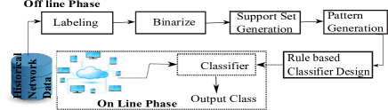
Figure 1: Block Diagram of the proposed SSIDS

V Performance Evaluations

Most widely used datasets for validation of IDSs are NSL-KDD [18] and KDDCUP’99 [14]. NSL-KDD is a modified version of the KDDCUP’99 dataset and we have used the NSL-KDD dataset in all our experiments. Both the datasets consist of $41$ features along with a class label for each observation. These features are categorized into four different classes and they are (i) basic features, (ii) content features, (iii) time-based traffic features, (iv) host-based traffic features. Here, the basic features are extracted from the TCP/IP connections without scanning the packets and there are nine such features in the NSL-KDD dataset. On the other hand, features which are extracted after inspecting the payloads of a TCP/IP connection are known as the content features and there are $13$ such features present in the dataset. A detailed description of the features is available in the Table VII. There are different types of attacks present in the dataset but we have clubbed them to one and consider them as “attack” only. Thus, there are two types of class labels that we have considered in our experiments and they are “normal” and “attack”. We have used the KDDTrain_20percent dataset which is a part of the NSL-KDD dataset to build the classifier in the offline phase. The KDDTest⁺ and the KDDTest^-21 have been used during the online phase for validation testing. The details of the experimental setup are presented in Subsection V-A.

Feature Type	Col. No	Input Feature	Data Type	Feature Type	Col. No	Input Feature	Data Type
	1	duration	C		23	Count	C
	2	protocol_type	S		24	srv_count	C
	3	service	S	Traffic (Time Based)	25	serror_rate	C
Basic	4	flag	S		26	srv_error_rate	C
	5	src_bytes	C		27	rerror_rate	C
	6	dst_bytes	C		28	srv_rerror_rate	C
	7	land	S		29	same_srv_rate	C
	8	wrong_fragment	C		30	diff_srv_rate	C
	9	urgent	C		31	srv_diff_host_rate	C
	10	hot	C		32	dst_host_count	C
	11	num_failed_logins	C		33	dst_host_srv_count	C
	12	logged_in	S	Traffic (Host Based)	34	dst_host_same_srv_rate	C
	13	num_compromised	C		35	dst_host_diff_srv_rate	C
	14	root_shell	C		36	dst_host_same_src_port_rate	C
Contents	15	su_attempted	C		37	dst_host_srv_diff_host_rate	C
	16	num_root	C		38	dst_host_serror_rate	C
	17	num_file_creations	C		39	dst_host_srv_serror_rate	C
	18	num_shells	C		40	dst_host_rerror_rate	C
	19	num_access_files	C		41	dst_host_srv_rerror_rate	C
	20	num_outbound_cmds	C
	21	is_hot_login	S	C means Continuous
	22	is_guest_login	S	S means Symbolic

TABLE VII: Input features of the NSL-KDD dataset.

V-A Experimental setup

The next step after the labels are generated is binarization. Detailed attention is needed to track the number of binary variables produced during this process. In the case of numeric or continuous features, the number of binary variables generated is directly dependent on the number of cut-points. Thus, if a feature is producing a large number of cut-points, it will increase the number of binary variables exponentially. For example, if the number of cut-points is $100$, the total number of interval variables is $\binom{100}{2}=4950$ and after considering the level variables, the total number of binary variables created will be $4950+100=5050$. Consequently, the memory requirement will increase afterward to an unmanageable level. On the other hand, a large number of cut-points indicate that the feature may not have much influence on the classification of observations. Our strategy is to ignore such features completely. Another set of features which are having a fairly large number of cut-points are ignored partially. Given a feature $x$, if the number of cut-points is greater than or equal to $175$, we completely ignore the feature $x$ and if the number of cut-points is greater than or equal to $75$ but less than $175$, we ignore that feature partially by only generating the level variables. We have arrived at these thresholds after empirical analysis using the training data. List of features that have been fully or partially ignored are presented in the Table VIII.

Col. Num.	Input feature	#Cut-points	Ignored ?
1	duration	102	Partially
5	src_bytes	116	Partially
23	Count	374	Fully
24	srv_count	302	Fully
32	dist_host_count	254	Fully
33	dist_host_srv_count	255	Fully
34	dst_host_same_srv_rate	100	Partially
35	dst_host_diff_srv_rate	93	Partially
36	dst_host_same_src_port_rate	100	Partially
38	dst_host_serror_rate	98	Partially
40	dst_host_rerror_rate	100	Partially

TABLE VIII: Binarization: Ignored features of the NSL-KDD dataset.

Another important aspect that we have incorporated into our design is the support of a pattern. Support of a positive (negative) pattern is $k$ if it covers $k$ positive (negative) observations and it should not cover any negative (positive) observation. Thus, the value of $k$ in Step 22 of Algorithm 1 holds immense importance. In a previous implementation [6] the value of $k=1$ have been used, but it is observed during experiments that such a low support is generating a lot of patterns/rules having little practical significance. Moreover, these patterns cause a lot of false positives during testing. An empirical analysis helps us to fix the threshold at $k=100$. At this threshold, more than $95\%$ of the observations present in the training dataset are covered by the generated patterns having degree up to $4$.

1:Input: Observation $obs$ having $41$ features.

2:Output: Class label $\mathcal{L}$.

3:if $\neg(obs(36)\geq 0.0050)\land(obs(37)\geq 0.0050\land obs(37)<0.1150)$ then

4:  $\mathcal{L}=1$ - $\mathcal{L}=1$ indicates normal behavior.

5:else if $obs(5)\geq 28.50\land\neg(obs(37)\geq 0.005\land obs(37)<0.915)\land strcmp(obs(r,3),^{\prime}ftp\_data^{\prime})$ then

6:  $\mathcal{L}=1$

7:else if $obs(5)\geq 28.5000\land(obs(37)\geq 0.0050\land obs(37)<0.9150)\land obs(34)\geq 0.1950$ then

8:  $\mathcal{L}=1$

9:else if $obs(5)\geq 28.500000\land\neg(obs(5)\geq 333.500000)\land obs(37)\geq 0.005000\land obs(37)<0.085000$ then

10:  $\mathcal{L}=1$

11:else if $obs(5)\geq 28.500000\land\neg(obs(34)\geq 0.645000)\land strcmp(obs(r,3),^{\prime}ftp\_data^{\prime})$ then

12:  $\mathcal{L}=1$

13:else if $obs(6)\geq 0.500000\land obs(37)\geq 0.005000\land obs(37)<0.915000\land\neg(obs(40)\geq 0.005000)$ then

14:  $\mathcal{L}=1$

15:else if $obs(6)\geq 0.500000\land\neg(obs(5)\geq 333.500000)\land obs(5)\geq 181.500000$ then

16:  $\mathcal{L}=1$

17:else if $obs(5)\geq 333.500000\land(obs(36)\geq 0.015000)\land obs(6)\geq 0.500000\land obs(6)<8303.000000$ then

18:  $\mathcal{L}=1$

19:else if $obs(5)\geq 333.500000\land obs(34)\geq 0.645000\land obs(6)\geq 0.500000\land obs(6)<8303.000000$ then

20:  $\mathcal{L}=1$

21:else if $\neg(obs(40)\geq 0.005000)\land obs(34)\geq 0.645000\land\neg(obs(36)\geq 0.005000)$ then

22:  $\mathcal{L}=1$

23:else if $\neg(obs(40)\geq 0.005000)\land obs(6)\geq 0.500000\land obs(6)<8303.000000\land\neg(obs(34)\geq 0.045000)$ then

24:  $\mathcal{L}=1$

25:else if $obs(5)\geq 28.50\land obs(6)\geq 0.500\land obs(36)\geq 0.015000\land\neg(obs(10)\geq 0.500000\land obs(10)<29.000000)$ then

26:  $\mathcal{L}=1$

27:else if $obs(5)\geq 28.50\land obs(6)\geq 0.500\land\neg(obs(40)\geq 0.005000)\land\neg(obs(10)\geq 0.500000\land obs(10)<29.000000)$ then

28:  $\mathcal{L}=1$

29:else

30:  $\mathcal{L}=0$ - $\mathcal{L}=0$ indicates attack.

31:end if

Classifier 1 Details of SSIDS

V-B Experimental Results

We have described all the steps required to design a classifier in the offline phase. Let us now summarize the outcome of the individual steps.
1. Labeling: We have used $5000$ labeled observations for labeling $20192$ unlabeled observations as described in Section III. This step produces $22601$ labeled observations which have been used in the following steps to design the classifier.
2. Binarize: During this step, total $10306$ binary variables are produced and a binary dataset along with its class labels having size $22601\times 10307$ is generated.
3. Support Set Generation: We have selected $21$ binary features according to their discriminating power.
4. Pattern Generation: During pattern generation, we found $13$ positive and $7$ negative patterns.
5. Classifier Design: We have developed a rule-based IDS using the $13$ positive patterns that are generated in the last step. Thus, the SSIDS contains $13$ rules. The details of the SSIDS is available in the Classifier 1. The NSL-KDD dataset contains two test datasets: (i) KDDTest⁺ having $22,544$ observations, and (ii) KDDTest²¹ having $11,850$ observations. These two datasets are used to measure the accuracy of the proposed SSIDS and the results related to the accuracy of the IDS is presented in Table IX. These results compare favorably with the state of the art classifiers proposed in [4], and the comparative results are presented in Table X. It is evident that the proposed SSIDS outperforms the existing IDSs by a wide margin.

Dataset	Accuracy	Precision	Sensitivity	F1-Score	Time in sec.
KDDTest+	90.91%	0.9458	0.8915	0.9179	0.000156
KDDTest21	83.92%	0.9417	0.8564	0.8971	0.000173

TABLE IX: Results related to KDDTest⁺ and KDDTest²¹.

Classifiers$	Accuracy using Dataset(%)
	KDDTest+	KDDTest21
J48*	81.05	63.97
Naive Bayes*	76.56	55.77
NB Tree*	82.02	66.16
Random forests*	80.67	63.25
Random Tree*	81.59	58.51
Multi-layer perceptron*	77.41	57.34
SVM*	69.52	42.29
Experiment-1 of  [4]	82.41	67.06
Experiment-2 of  [4]	84.12	68.82
LAD@	87.42	79.09
Proposed SSIDS	90.91	83.92
*  Results as reported in [4].
@ Classifier designed using dataset DL only by
omitting the ‘labeling’ process.
$  All the classifiers use the same training
dataset, i.e., KDDTrain_20percent.

TABLE X: Performance Comparison between different Classifiers, IDSs and the proposed SSIDS.

VI Conclusion

The intrusion detection system (IDS) is a critical tool used to detect cyber attacks, and semi-supervised IDSs are gaining popularity as it can enrich its knowledge-base from the unlabeled observations also. Discovering and understanding the usage patterns from the past observations play a significant role in the detection of network intrusions by the IDSs. Normally, usage patterns establish a causal relationship among the observations and their class labels and the LAD is useful for such problems where we need to automatically generate useful patterns that can predict the class labels of future observations. Thus, LAD is ideally suited to solve the design problems of IDSs. However, the dearth of labeled observations makes it difficult to use the LAD in the design of IDSs, particularly semi-supervised IDSs, as we need to consider the unlabeled examples along with the labeled examples during the design of IDSs. In this effort, we have proposed a simple methodology to extend the classical LAD to consider unlabeled observations along with the labeled observations. We have employed the proposed technique successfully to design a new semi-supervised “Intrusion Detection System” which outperforms the existing semi-supervised IDSs by a wide margin both in terms of accuracy and detection time.

Appendix

$A\geq 3.05$	$A\geq 2.45$	$A\geq 1.65$	$1.65\leq A<3.05$	$2.45\leq A<3.05$	$1.65\leq A<2.45$	$B\geq 2.95$	$B\geq 1.85$	$1.85\leq B<2.95$	$C\geq 4.5$	$C\geq 3.3$	$C\geq 1.9$	$1.9\leq C<4.5$	$1.9\leq C<3.3$	$3.3\leq C<4.5$	Class
$b_{1}$	$b_{2}$	$b_{3}$	$b_{4}$	$b_{5}$	$b_{6}$	$b_{7}$	$b_{8}$	$b_{9}$	$b_{10}$	$b_{11}$	$b_{12}$	$b_{13}$	$b_{14}$	$b_{15}$	$\mathcal{L}$
1	1	1	0	0	0	1	1	0	0	0	1	1	1	0	1
0	1	1	1	1	0	0	0	0	1	1	1	0	0	0	1
0	0	0	0	0	0	0	1	1	0	1	1	1	0	1	1
1	1	1	0	0	0	0	0	0	0	1	1	1	0	1	0
0	0	1	1	0	1	0	1	1	0	0	0	0	0	0	0

TABLE XI: Binary dataset generated from the Table V having $15$ binary variables from $b_{1}$ to $b_{15}$.

References

- [1] G. Alexe, S. Alexe, T. O. Bonates, and A. Kogan, “Logical analysis of data – the vision of peter l. hammer,” Annals of Mathematics and Artificial Intelligence, vol. 49, no. 1, pp. 265–312, Apr 2007.
- [2] H. Almuallim and T. G. Dietterich, “Learning boolean concepts in the presence of many irrelevant features,” Artificial Intelligence, vol. 69, pp. 279–305, 1994.
- [3] M. A. Ambusaidi, X. He, P. Nanda, and Z. Tan, “Building an intrusion detection system using a filter-based feature selection algorithm,” IEEE Transactions on Computers, vol. 65, no. 10, pp. 2986–2998, 2016.
- [4] R. A. R. Ashfaq, X.-Z. Wang, J. Z. Huang, H. Abbas, and Y.-L. He, “Fuzziness based semi-supervised learning approach for intrusion detection system,” Information Sciences, vol. 378, pp. 484 – 497, 2017.
- [5] E. Boros, P. L. Hammer, T. Ibaraki, and A. Kogan, “Logical analysis of numerical data,” Mathematical Programming, vol. 79, no. 1, pp. 163–190, Oct 1997.
- [6] E. Boros, P. L. Hammer, T. Ibaraki, A. Kogan, E. Mayoraz, and I. Muchnik, “An implementation of logical analysis of data,” IEEE Trans. on Knowl. and Data Eng., vol. 12, no. 2, pp. 292–306, Mar. 2000.
- [7] R. Bruni and G. Bianchi, “Effective classification using a small training set based on discretization and statistical analysis,” IEEE Transactions on Knowledge and Data Engineering, vol. 27, no. 9, pp. 2349–2361, Sep. 2015.
- [8] R. Bruni, G. Bianchi, C. Dolente, and C. Leporelli, “Logical analysis of data as a tool for the analysis of probabilistic discrete choice behavior,” Computers & Operations Research, 2018.
- [9] Y. Crama, P. Hammer, and T. Ibaraki, “Cause-effect relationships and partially defined boolean functions,” Ann. Oper. Res., vol. 16, no. 1-4, pp. 299–325, Jan. 1988.
- [10] T. K. Das, S. Ghosh, E. Koley, and J. Zhou, “Design of a fdia resilient protection scheme for power networks by securing minimal sensor set,” in Proceedings of 2019 International Workshop on Artificial Intelligence and Industrial Internet-of-Things Security, LNCS-11605, 2019.
- [11] D. E. Denning, “An intrusion-detection model,” IEEE Transactions on Software Engineering, vol. SE-13, no. 2, pp. 222–232, Feb 1987.
- [12] P. Hammer, “Partially defined boolean functions and cause-effect relationships,” in International Conference on Multi-attribute Decision Making Via OR-based Expert Systems. University of Passau, Passau, Germany, April 1986.
- [13] E. Hernández-Pereira, J. A. Suárez-Romero, O. Fontenla-Romero, and A. Alonso-Betanzos, “Conversion Methods for Symbolic Features: A comparison applied to an Intrusion Detection Problem,” Expert Systems with Applications, vol. 36, no. 7, pp. 10 612–10 617, 2009.
- [14] KDD, “Kdd cup 1999 data,” http://kdd.ics.uci.edu/databases/kddcup99/kddcup99.html, 1999, [Online; accessed 05-July-2018].
- [15] G. Kim, S. Lee, and S. Kim, “A novel hybrid intrusion detection method integrating anomaly detection with misuse detection,” Expert Systems with Applications, vol. 41, no. 4, Part 2, pp. 1690 – 1700, 2014.
- [16] H.-J. Liao, C.-H. R. Lin, Y.-C. Lin, and K.-Y. Tung, “Intrusion detection system: A comprehensive review,” Journal of Network and Computer Applications, vol. 36, no. 1, pp. 16 – 24, 2013.
- [17] S. Mukkamala, A. H. Sung, and A. Abraham, “Intrusion detection using an ensemble of intelligent paradigms,” J. Netw. Comput. Appl., vol. 28, no. 2, pp. 167–182, Apr. 2005.
- [18] M. Tavallaee, E. Bagheri, W. Lu, and A. A. Ghorbani, “A detailed analysis of the kdd cup 99 data set,” in Proceedings of the Second IEEE International Conference on Computational Intelligence for Security and Defense Applications, ser. CISDA’09. Piscataway, NJ, USA: IEEE Press, 2009, pp. 53–58.
- [19] C.-F. Tsai, Y.-F. Hsu, C.-Y. Lin, and W.-Y. Lin, “Intrusion detection by machine learning: A review,” Expert Systems with Applications, vol. 36, no. 10, pp. 11 994 – 12 000, 2009.
- [20] H. Wang, J. Gu, and S. Wang, “An effective intrusion detection framework based on svm with feature augmentation,” Knowledge-Based Systems, vol. 136, pp. 130 – 139, 2017.
- [21] Q. Yan and F. R. Yu, “Distributed denial of service attacks in software-defined networking with cloud computing,” IEEE Communications Magazine, vol. 53, no. 4, pp. 52–59, April 2015.
- [22] X. Zhu and A. B. Goldberg, “Introduction to semi-supervised learning,” Synthesis Lectures on Artificial Intelligence and Machine Learning, vol. 3, no. 1, pp. 1–130, 2009.