Direct estimation of the energy gap between the ground state and excited state with quantum annealing

Abstract

Quantum chemistry is one of the important applications of quantum information technology. Especially, an estimation of the energy gap between a ground state and excited state of a target Hamiltonian corresponding to a molecule is essential. In the previous approach, an energy of the ground state and that of the excited state are estimated separately, and the energy gap can be calculated from the subtraction between them. Here, we propose a direct estimation of the energy gap between the ground state and excited state of the target Hamiltonian with quantum annealing. The key idea is to combine a Ramsey type measurement with the quantum annealing. This provides an oscillating signal with a frequency of the energy gap, and a Fourier transform of the signal let us know the energy gap. Based on typical parameters of superconducting qubits, we numerically investigate the performance of our scheme when we estimate an energy gap between the ground state and first excited state of the Hamiltonian. We show robustness against non-adiabatic transitions between the ground state and first-excited state. Our results pave a new way to estimate the energy gap of the Hamiltonian for quantum chemistry.

I Introduction

Quantum annealing (QA) has been studied as a way to solve combinational optimization problems Kadowaki and Nishimori (1998); Farhi et al. (2000, 2001) where the goal is to minimize a cost function. Such a problem is mapped into a finding of a ground state of Ising Hamiltonians that contain the information of the problem. QA is designed to find an energy eigenstate of the target Hamiltonian by using adiabatic dynamics. So, by using the QA, we can find the ground state of the Ising Hamiltonian for the combinational optimization problem.

D-Wave systems, Inc. has have realized a quantum device to implement the QA Johnson et al. (2011). Superconducting flux qubits Orlando et al. (1999); Mooij et al. (1999); Harris et al. (2010) have been used in the device for the QA. Since superconducting qubits are artificial atoms, there are many degree of freedoms to control parameters by changing the design and external fields, which is suitable for a programmable device. QA with the D-Wave machines can be used not only for finding the ground state, but also for quantum simulations Harris et al. (2018); King et al. (2018) and machine learning Mott et al. (2017); Amin et al. (2018).

Quantum chemistry is one of the important applications of quantum information processing Levine et al. (2009); Serrano-Andrés and Merchán (2005); McArdle et al. (2020), and it was recently shown that the QA can be also used for quantum chemistry calculations Perdomo-Ortiz et al. (2012); Aspuru-Guzik et al. (2005); Lanyon et al. (2010); Du et al. (2010); Peruzzo et al. (2014); Mazzola et al. (2017); Streif et al. (2019); Babbush et al. (2014). Important properties of molecules can be investigated by the second quantized Hamiltonian of the molecules. Especially, the energy gap between the ground state and excited states is essential information for calculating optical spectra and reaction rates  Serrano-Andrés and Merchán (2005). The second quantized Hamiltonian can be mapped into the Hamiltonian of qubits Jordan and Wigner (1928); Bravyi and Kitaev (2002); Aspuru-Guzik et al. (2005); Seeley et al. (2012); Tranter et al. (2015). Importantly, not only the ground state but also the excited state of the Hamiltonian can be prepared by the QA Chen et al. (2019); Seki et al. (2020). By measuring suitable observable on such states prepared by the QA, we can estimate the eigenenergy of the Hamiltonian. In the conventional approaches, we need to perform two separate experiments to estimate an energy gap between the ground state and the excited state. In the first (second) experiment, we measure the eigenenergy of the ground (excited) state prepared by the QA. From the subtraction between the estimation of the eigenenergy of the ground state and that of the excited state, we can obtain the information of the energy gap Seki et al. (2020).

Here, we propose a way to estimate an energy gap between the ground state and excited state in a more direct manner. The key idea is to use the Ramsey type measurement where a superposition between the ground state and excited state acquires a relative phase that depends on the energy gap Ramsey (1950). By performing the Fourier transform of the signal from the Ramsey type experiments, we can estimate the energy gap. We numerically study the performance of our protocol to estimate the energy gap between the ground state and first excited state. We show robustness of our scheme against non-adiabatic transitions between the ground state and first excited state.

II Estimation of the energy gap between the ground state and excited state based on the Ramsey type measurement

We use the following time-dependent Hamiltonian in our scheme

$$H = A(t)H_{\rm{D}}+(1-A(t))H_{\rm{P}}$$

$$A(t) = \left\{\begin{array}[]{ll}1-\frac{t}{T}&(0\leq t\leq T)\\ 0&(T\leq t\leq T+\tau)\\ \frac{t-(T+\tau)}{T}&(T+\tau\leq t\leq 2T+\tau)\\ \end{array}\right.$$ (4)

where $A(t)$ denotes an external control parameter (as shown in the Fig. 1), $H_{\rm{D}}$ denotes the driving Hamiltonian that is typically chosen as the transverse magnetic field term, and $H_{\rm{P}}$ denotes the target (or problem) Hamiltonian whose energy gap we want to know. This means that, depending on the time period, we have three types of the Hamiltonian as follows

$$H_{\rm{QA}} = (1-\frac{t}{T})H_{\rm{D}}+\frac{t}{T}H_{\rm{P}}$$

$$H_{\rm{R}} = H_{\rm{P}}$$

$$H_{\rm{RQA}} = \frac{t-(T+\tau)}{T}H_{\rm{D}}+(1-\frac{t-(T+\tau)}{T})H_{\rm{P}}$$

In the first time period of $0\leq t\leq T$, the Hamiltonian is $H_{\rm{QA}}$, and this is the same as that is used in the standard QA. In the next time period of $T\leq t\leq T+\tau$, the Hamiltonian becomes $H_{\rm{R}}$, and the dynamics induced by this Hamiltonian corresponds to that of the Ramsey type evolution Ramsey (1950) where the superposition of the state acquires a relative phase depending on the energy gap. In the last time period of $T+\tau\leq t\leq 2T+\tau$, the Hamiltonian becomes $H_{\rm{RQA}}$, and this has a similar form of that is used in a reverse QA Perdomo-Ortiz et al. (2011); Ohkuwa et al. (2018); Yamashiro et al. (2019); Arai et al. (2020).

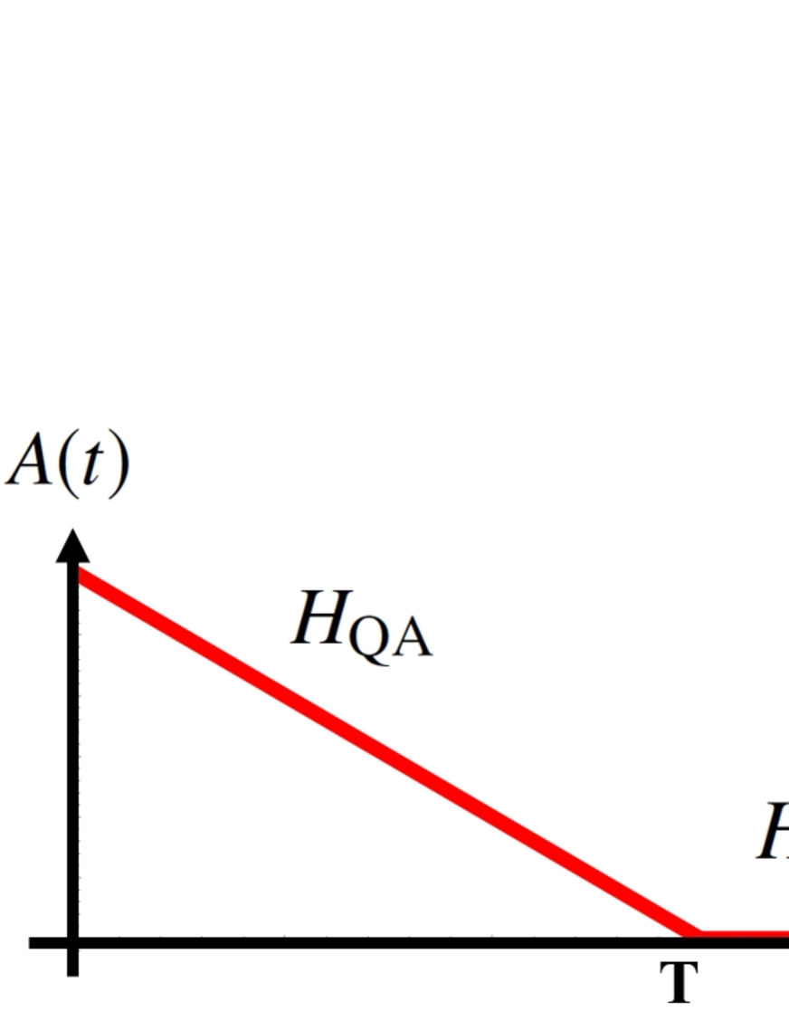
Figure 1: An external control parameter $A(t)$ of our time-dependent Hamiltonian $H(t)=A(t)H_{\rm{D}}+(1-A(t))H_{\rm{P}}$ where $H_{\rm{D}}$ denotes the driving Hamiltonian and $H_{\rm{P}}$ denotes the target (problem) Hamiltonian. With a time period of $0\leq t\leq T$, we have the Hamiltonian $H_{\rm{QA}}$ that is used in the standard QA. With the next time period of $T\leq t\leq T+\tau$, we have the Ramsey time Hamiltonian $H_{\rm{R}}$ where the quantum state acquires a relative phase induced from the energy gap. In the final time period of $T+\tau\leq t\leq 2T+\tau$, we have the Hamiltonian $H_{\rm{RQA}}$ which is used in a reverse QA. By using the dynamics induced by these Hamiltonians, we can estimate the energy gap of the target Hamiltonian.

We explain the details of our scheme. Firstly, prepare an initial state of $|\psi_{0}\rangle=\frac{1}{\sqrt{2}}(|E_{0}^{\rm{(D)}}\rangle+|E_{1}^{\rm{(D)}}\rangle)$ where $|E_{0}^{\rm{(D)}}\rangle$ ($|E_{1}^{\rm{(D)}}\rangle$) denotes the ground (excited) state of the driving Hamiltonian. Secondly, let this state evolve in an adiabatic way by the Hamiltonian of $H_{\rm{QA}}$ and we obtain a state of $\frac{1}{\sqrt{2}}(|E_{0}^{\rm{(P)}}\rangle+e^{-i\theta}|E_{1}^{\rm{(P)}}\rangle)$ where $|E_{0}^{\rm{(P)}}\rangle$ ($|E_{1}^{\rm{(P)}}\rangle$) denotes the ground (excited) state of the target Hamiltonian and $\theta$ denotes a relative phase acquired during the dynamics. Thirdly, let the state evolve by the Hamiltonian of $H_{\rm{R}}$ for a time $T\leq t\leq T+\tau$, and we obtain $\frac{1}{\sqrt{2}}(|E_{0}^{\rm{(P)}}\rangle+e^{-i\Delta E\tau-i\theta}|E_{1}^{\rm{(P)}}\rangle)$ where $\Delta E=E_{1}^{(\rm{P})}-E_{0}^{(\rm{P})}$ denotes an energy gap and $E_{0}^{(\rm{P})}$ ($E_{1}^{(\rm{P})}$) denotes the eigenenergy of the ground (first excited) state of the target Hamiltonian. Fourthly, let this state evolve in an adiabatic way by the Hamiltonian of $H_{\rm{RQA}}$ from $t=T+\tau$ to $T$, and we obtain a state of $\frac{1}{\sqrt{2}}(|E_{0}^{\rm{(D)}}\rangle+e^{-i\Delta E\tau-i\theta^{\prime}}|E_{1}^{\rm{(D)}}\rangle)$ where $\theta^{\prime}$ denotes a relative phase acquired during the dynamics. Fifthly, we readout the state by using a projection operator of $|\psi_{0}\rangle\langle\psi_{0}|$, and the projection probability is $P_{\tau}=\frac{1}{2}+\frac{1}{2}\cos(\Delta E\tau+\theta^{\prime})$, which is an oscillating signal with a frequency of the energy gap. Finally, we repeat the above five steps by sweeping $\tau$, and obtain several values of $P_{\tau}$. We can perform the Fourier transform of $P_{\tau}$ such as

$$f(\omega)=\sum_{n=1}^{N}(P_{\tau}-\frac{1}{2})e^{-i\omega\tau_{n}}$$ (5)

where $\tau_{n}=t_{\rm{min}}+\frac{n-1}{(N-1)}(t_{\rm{max}}-t_{\rm{min}})$ denotes a time step, $t_{\rm{min}}$ ($t_{\rm{max}}$) denotes a minimum (maximum) time to be considered, and $N$ denotes the number of the steps. The peak in $f(\omega)$ shows the energy gap $\Delta E$.

Figure 2: Fourier function against a frequency. Here, we set parameters as $\lambda_{1}/2\pi=1$ GHz, $g/2\pi=0.5$ GHz, $\omega_{1}/2\pi=0.2$ GHz, $\omega_{2}/\omega_{1}=1.2$, $g^{\prime}/g=2.1$, $\lambda_{2}/\lambda_{1}=10.7$, $L=2$, $N=10000$, $t_{\rm{min}}=0$, $t_{\rm{max}}=100$ ns. (a) We set $T=150\ (75)$ ns for the blue (red) plot, where we have a peak around $1.067$ GHz, which corresponds to the energy difference between the ground state and first excited state of the target Hamiltonian. We have another peak around $\omega=0$, and this comes from non-adiabatic transition during the QA. (b) We set $T=37.5$($12.5$) ns for the blue (red) plot. We have an additional peak around $1.698$ GHz ($2.7646$ GHz), which corresponds to the energy difference between the first excited state (ground state) and second excited state of the target Hamiltonian.

To check the efficiency, we perform the numerical simulations to estimate the energy gap between the ground state and first excited state, based on typical parameters for superconducting qubits. We choose the following Hamiltonians

$$H_{\rm{D}} = \sum_{j=1}^{L}\frac{\lambda_{j}}{2}\hat{\sigma}_{x}^{(j)}$$

$$H_{\rm{P}} = \sum_{j=1}^{L}\frac{\omega_{j}}{2}\hat{\sigma}_{z}^{(j)}+\sum_{j=1}^{L-1}g\hat{\sigma}_{z}^{(j)}\hat{\sigma}_{z}^{(j+1)}+g^{\prime}(\hat{\sigma}_{+}^{(j)}\hat{\sigma}_{-}^{(j+1)}+\hat{\sigma}_{-}^{(j)}\hat{\sigma}_{+}^{(j+1)})$$ (6)

where $\lambda_{j}$ denotes the amplitude of the transverse magnetic fields of the $j$-th qubit, $\omega_{j}$ denotes the frequency of the $j$-th qubit, and $g$($g^{\prime}$) denotes the Ising (flip-flop) type coupling strength between qubits.

We consider the case of two qubits, and the initial state is $|1\rangle|-\rangle$ where $|1\rangle$ ($|-\rangle$) is an eigenstate of $\hat{\sigma}_{z}$($\hat{\sigma}_{x}$) with an eigenvalue of +1 (-1). In the Fig. 2 (a), we plot the Fourier function $|f(\omega)|$ against $\omega$ for this case. When we set $T=150$ (ns) or $75$ (ns), we have a peak around $\omega=1.067$ GHz, which corresponds to the energy gap $\Delta E$ of the problem Hamiltonian in our parameter. So this result shows that we can estimate the energy gap by using our scheme. Also, we have a smaller peak of around $\omega=0$ in the Fig. 2 (a), and this comes from non-adiabatic transitions between the ground state and first excited state. If the dynamics is perfectly adiabatic, the population of both the ground state and first excited state should be $\frac{1}{2}$ at $t=T$. However, in the parameters with $T=150$ ($T=75$) ns, the population of the ground state and excited state is around 0.6 (0.7) and 0.4 (0.3) at $t=T$, respectively. In this case, the probability at the readout step should be modified as $P^{\prime}_{\tau}=a+b\cos(\Delta E\tau+\theta^{\prime})$ where the parameters $a$ and $b$ deviates from $\frac{1}{2}$ due to the non-adiabatic transitions. This induces the peak of around $\omega=0$ in the Fourier function $f(\omega)$. As we decrease $T$, the dynamics becomes less adiabatic, and the peak of $\omega=0$ becomes higher while the target peak corresponding the energy gap $\Delta E$ becomes smaller as shown in the Fig. 1. Importantly, we can still identify the peak corresponding to the energy gap for the following reasons. First, there is a large separation between the peaks. Second, the non-adiabatic transitions between the ground state and first excited state do not affect the peak position. So our scheme is robust against the non-adiabatic transition between the ground state and first excited state. This is stark contrast with a previous scheme that is fragile against such non-adiabatic transitions Seki et al. (2020).

Moreover, we have two more peaks in the Fig. 2 (b) where we choose $T=37.5$($12.5$) ns for the red (blue) plot, which is shorter than that of the Fig. 2 (a). The peaks are around $1.698$ GHz and $2.7646$ GHz, respectively. The former (latter) peak corresponds to the energy difference between the first excited state (ground state) and second excited state. We can interpret these peaks as follows. Due to the non-adiabatic dynamics, not only the first excited state but also the second excited state is induced in this case. The state after the evolution with $H_{\rm{R}}$ at $t=T+\tau$ is approximately given as a superposition between the ground state, the first excited state, and the second excited state such as $c_{0}e^{-iE_{0}^{\rm{(P)}}\tau-i\theta_{0}}|E_{0}^{\rm{(P)}}\rangle+c_{1}e^{-iE_{1}^{\rm{(P)}}\tau-i\theta_{1}}|E_{1}^{\rm{(P)}}\rangle+c_{2}e^{-iE_{2}^{\rm{(P)}}\tau-i\theta_{2}}|E_{2}^{\rm{(P)}}\rangle$ where $c_{i}$ $(i=0,1,2)$ denote real values and $\theta_{i}$ ($i=0,1,2$) denotes the relative phase induced by the QA. So the Fourier transform of the probability distribution obtained from the measurements provides us with three frequencies such as $(E_{0}^{\rm{(P)}}-E_{1}^{\rm{(P)}})$, $(E_{1}^{\rm{(P)}}-E_{2}^{\rm{(P)}})$, and $(E_{2}^{\rm{(P)}}-E_{0}^{\rm{(P)}})$. In the actual experiment, we do not know which peak corresponds to the energy gap between the ground state and first excited state, because there are other relevant peaks. However, it is worth mentioning that we can still obtain some information of the energy spectrum (or energy eigenvalues of the Hamiltonian) from the experimental data, even under the effect of the non-adiabatic transitions between the ground state and other excited states. Again, this shows the robustness of our scheme against the non-adiabatic transitions compared with the previous schemes Seki et al. (2020).

III Conclusion

In conclusion, we propose a scheme that allows the direct estimation of an energy gap of the target Hamiltonian by using quantum annealing (QA). While a ground state of a driving Hamiltonian is prepared as an initial state for the conventional QA, we prepare a superposition between a ground state and the first excited state of the driving Hamiltonian as the initial state. Also, the key idea in our scheme is to use a Ramsey type measurement after the quantum annealing process where information of the energy gap is encoded as a relative phase between the superposition. The readout of the relative phase by sweeping the Ramsey measurement time duration provides a direct estimation of the energy gap of the target Hamiltonian. We show that, unlike the previous scheme, our scheme is robust against non-adiabatic transitions. Our scheme paves an alternative way to estimate the energy gap of the target Hamiltonian for applications of quantum chemistry.

While this manuscript was being written, an independent article also proposes to use a Ramsey measurement to estimate an energy gap by using a quanutm device Russo et al. (2020).

This paper is partly based on results obtained from a project commissioned by the New Energy and Industrial Technology Development Organization (NEDO), Japan. This work was also supported by Leading Initiative for Excellent Young Researchers MEXT Japan, JST presto (Grant No. JPMJPR1919) Japan , KAKENHI Scientific Research C (Grant No. 18K03465), and JST-PRESTO (JPMJPR1914).

References

- Kadowaki and Nishimori (1998) T. Kadowaki and H. Nishimori, Physical Review E 58, 5355 (1998).
- Farhi et al. (2000) E. Farhi, J. Goldstone, S. Gutmann, and M. Sipser, arXiv preprint quant-ph/0001106 (2000).
- Farhi et al. (2001) E. Farhi, J. Goldstone, S. Gutmann, J. Lapan, A. Lundgren, and D. Preda, Science 292, 472 (2001).
- Johnson et al. (2011) M. W. Johnson, M. H. Amin, S. Gildert, T. Lanting, F. Hamze, N. Dickson, R. Harris, A. J. Berkley, J. Johansson, P. Bunyk, et al., Nature 473, 194 (2011).
- Orlando et al. (1999) T. Orlando, J. Mooij, L. Tian, C. H. Van Der Wal, L. Levitov, S. Lloyd, and J. Mazo, Physical Review B 60, 15398 (1999).
- Mooij et al. (1999) J. Mooij, T. Orlando, L. Levitov, L. Tian, C. H. Van der Wal, and S. Lloyd, Science 285, 1036 (1999).
- Harris et al. (2010) R. Harris, J. Johansson, A. Berkley, M. Johnson, T. Lanting, S. Han, P. Bunyk, E. Ladizinsky, T. Oh, I. Perminov, et al., Physical Review B 81, 134510 (2010).
- Harris et al. (2018) R. Harris, Y. Sato, A. Berkley, M. Reis, F. Altomare, M. Amin, K. Boothby, P. Bunyk, C. Deng, C. Enderud, et al., Science 361, 162 (2018).
- King et al. (2018) A. D. King, J. Carrasquilla, J. Raymond, I. Ozfidan, E. Andriyash, A. Berkley, M. Reis, T. Lanting, R. Harris, F. Altomare, et al., Nature 560, 456 (2018).
- Mott et al. (2017) A. Mott, J. Job, J.-R. Vlimant, D. Lidar, and M. Spiropulu, Nature 550, 375 (2017).
- Amin et al. (2018) M. H. Amin, E. Andriyash, J. Rolfe, B. Kulchytskyy, and R. Melko, Physical Review X 8, 021050 (2018).
- Levine et al. (2009) I. N. Levine, D. H. Busch, and H. Shull, Quantum chemistry, Vol. 6 (Pearson Prentice Hall Upper Saddle River, NJ, 2009).
- Serrano-Andrés and Merchán (2005) L. Serrano-Andrés and M. Merchán, Journal of Molecular Structure: THEOCHEM 729, 99 (2005).
- McArdle et al. (2020) S. McArdle, S. Endo, A. Aspuru-Guzik, S. C. Benjamin, and X. Yuan, Reviews of Modern Physics 92, 015003 (2020).
- Perdomo-Ortiz et al. (2012) A. Perdomo-Ortiz, N. Dickson, M. Drew-Brook, G. Rose, and A. Aspuru-Guzik, Scientific Reports 2, 571 (2012).
- Aspuru-Guzik et al. (2005) A. Aspuru-Guzik, A. D. Dutoi, P. J. Love, and M. Head-Gordon, Science 309, 1704 (2005).
- Lanyon et al. (2010) B. P. Lanyon, J. D. Whitfield, G. G. Gillett, M. E. Goggin, M. P. Almeida, I. Kassal, J. D. Biamonte, M. Mohseni, B. J. Powell, M. Barbieri, et al., Nature chemistry 2, 106 (2010).
- Du et al. (2010) J. Du, N. Xu, X. Peng, P. Wang, S. Wu, and D. Lu, Physical review letters 104, 030502 (2010).
- Peruzzo et al. (2014) A. Peruzzo, J. McClean, P. Shadbolt, M.-H. Yung, X.-Q. Zhou, P. J. Love, A. Aspuru-Guzik, and J. L. O’brien, Nature communications 5, 4213 (2014).
- Mazzola et al. (2017) G. Mazzola, V. N. Smelyanskiy, and M. Troyer, Physical Review B 96, 134305 (2017).
- Streif et al. (2019) M. Streif, F. Neukart, and M. Leib, in International Workshop on Quantum Technology and Optimization Problems (Springer, 2019) pp. 111–122.
- Babbush et al. (2014) R. Babbush, P. J. Love, and A. Aspuru-Guzik, Scientific Reports 4, 6603 (2014).
- Jordan and Wigner (1928) P. Jordan and E. Wigner, Z. Physik 47, 631 (1928).
- Bravyi and Kitaev (2002) S. B. Bravyi and A. Y. Kitaev, Annals of Physics 298, 210 (2002).
- Seeley et al. (2012) J. T. Seeley, M. J. Richard, and P. J. Love, The Journal of Chemical physics 137, 224109 (2012).
- Tranter et al. (2015) A. Tranter, S. Sofia, J. Seeley, M. Kaicher, J. McClean, R. Babbush, P. V. Coveney, F. Mintert, F. Wilhelm, and P. J. Love, International Journal of Quantum Chemistry 115, 1431 (2015).
- Chen et al. (2019) M.-C. Chen, M. Gong, X.-S. Xu, X. Yuan, J.-W. Wang, C. Wang, C. Ying, J. Lin, Y. Xu, Y. Wu, et al., arXiv preprint arXiv:1905.03150 (2019).
- Seki et al. (2020) Y. Seki, Y. Matsuzaki, and S. Kawabata, arXiv preprint arXiv:2002.12621 (2020).
- Ramsey (1950) N. F. Ramsey, Physical Review 78, 695 (1950).
- Perdomo-Ortiz et al. (2011) A. Perdomo-Ortiz, S. E. Venegas-Andraca, and A. Aspuru-Guzik, Quantum Information Processing 10, 33 (2011).
- Ohkuwa et al. (2018) M. Ohkuwa, H. Nishimori, and D. A. Lidar, Physical Review A 98, 022314 (2018).
- Yamashiro et al. (2019) Y. Yamashiro, M. Ohkuwa, H. Nishimori, and D. A. Lidar, Physical Review A 100, 052321 (2019).
- Arai et al. (2020) S. Arai, M. Ohzeki, and K. Tanaka, arXiv preprint arXiv:2004.11066 (2020).
- Russo et al. (2020) A. E. Russo, K. M. Rudinger, B. C. A. Morrison, and A. D. Baczewski, arXiv:2007.08697 (2020).