Experiment data-driven modeling of tokamak discharge in EAST

Abstract

A model for tokamak discharge through deep learning has been done on a superconducting long-pulse tokamak (EAST). This model can use the control signals (i.e. Neutral Beam Injection (NBI), Ion Cyclotron Resonance Heating (ICRH), etc) to model normal discharge without the need for doing real experiments. By using the data-driven methodology, we exploit the temporal sequence of control signals for a large set of EAST discharges to develop a deep learning model for modeling discharge diagnostic signals, such as electron density $n_{e}$, store energy $W_{mhd}$ and loop voltage $V_{loop}$. Comparing the similar methodology, we use Machine Learning techniques to develop the data-driven model for discharge modeling rather than disruption prediction. Up to 95% similarity was achieved for $W_{mhd}$. The first try showed promising results for modeling of tokamak discharge by using the data-driven methodology. The data-driven methodology provides an alternative to physical-driven modeling for tokamak discharge modeling.

Keywords: tokamak, discharge modeling, machine learning

1 Introduction

A reliable model of tokamak is critical to magnetic confinement fusion experimental research. It is used to check the feasibility of pulse, interpret experimental data, validate the theoretical model, and develop control technology.

The conventional physical-driven modeling tools come from empirical models or derivations based on first principles, the so-called "Integrated Modeling" [1]. "Integrated Modeling" is a suite of module codes that address the different physical processes in the tokamak, i.e. core transport, equilibrium, stability, boundary physics, heating, fueling, and current drive. Typical workflows are ETS [1], PTRANSP [2], TSC [3], CRONOS [4], JINTRAC [5], METIS [6], ASTRA [7], TOPICS [8], etc. The reliability of the first-principles model depends on the completeness of the physical processes involved. In the past few decades, sophisticated physical modules have been developed and integrated into these codes for more realistic modeling results. Typical workflow for a full discharge modeling on tokamak is using sophisticated modules that integrate many physical processes [9, 1]. Due to the nonlinear, multi-scale, multi-physics characteristics of tokamak, high-fidelity simulation of the whole tokamak discharge process is still a great scientific challenge [10].

Increasingly, researchers are turning to data-driven approaches. The history can be traced back to the use of machine learning for interrupt prediction since the 1990s, i.e. ADITYA [11, 12], Alcator C-Mod [13, 14, 15], EAST [15, 16, 17], DIII-D [13, 18, 15, 19, 20, 21, 22, 23, 24, 25, 26, 27, 28, 16] JET [29, 22, 30, 31, 32, 33, 34, 35, 36, 28, 16], ASDEX-Upgrade[37, 38, 30, 39], JT-60U [40, 41], HL-2A [42, 43], NSTX [44] and J-TEXT [45, 46]. Neural-network-based models are also used to accelerate theory-based modeling [47, 48, 49]. In these works [47, 48, 49], one neural network was trained with a database of modeling and successfully reproduced approximate results with several orders of magnitude speedup. There are also many deep learning architectures have been created and successfully applied in sequence learning problems [27, 50, 51, 52, 36] in areas of time-series analysis or natural language processing. At present, most machine learning work in fusion community estimates the plasma state at each moment in time, usually identified as either non-disruptive or disruptive. However, compared with traditional physical modeling methods, it is far from enough to just predict whether the disruption will occur. We need to understand the evolution of the plasma state of tokamak and its response to external control during the discharge process.

Physics-driven approaches reconstruct physical high-dimensional reality from the bottom-up and then reduce them to the low-dimensional model. Alternatively, data-driven approaches discover the relationships between low-dimensional quantities from a large amount of data and then construct approximate models of the nonlinear dynamical system. When focusing only on the evolution of low-dimensional macroscopic features of complex dynamic systems, data-driven approaches can build models more efficiently. In practical applications, control signals and diagnostic signals of tokamak usually appear as temporal sequence of low-dimensional data, most of which are zero-dimensional or one-dimensional profiles and rarely two-dimensional distribution. If we consider tokamak as a black box, these signals can be considered as inputs and outputs of a dynamic system. Discharge modeling is to model the connection between the input and output signal. This can be understood as the conversion from one kind of time series data to another.

In the present work, a neural network model is trained with the temporal sequence of control signals and diagnostic signals for a large dataset of EAST discharges [53, 54, 55]. It can reproduce the response of the main diagnostic signals to control signals during the whole discharge process and predict their time evolution curves, such as electron density $n_{e}$, store energy $W_{mhd}$ and loop voltage $V_{loop}$.

The rest of this paper consists of five parts. Section 2 provides descriptions of data preprocessing and data selection criteria. Section 3 shows the model details of this work. The detailed model training process can be found in section 4. Then an in-depth analysis of the model results is put forward in section 5. Finally, a brief conclusion is made in section 6.

2 Dataset

EAST’s data system stores more than 3000 channels of raw acquisition signals and thousands of processed physical analysis data [56], which record the entire process of tokamak discharge. These data can be divided into three categories: configuration parameters, control signals, and diagnostic signals. The configuration parameters describe constants related to device construction, such as the shape of the vacuum chamber, the position of the poloidal magnetic field (PF) coils, etc. The control signals are the external constraints actively applied to the magnetic field coil and auxiliary heating systems, such as the current of PF coils, or the power of Lower Hybrid Wave (LHW), etc. The diagnostic signals are the physics information passively measured from the plasma, such as electron density $n_{e}$, or loop voltage $V_{loop}$, etc. The configuration parameters will not change during the experiment campaign, so there is no need to consider them unless a cross-device model is built. The discharge modeling is essentially a process of mapping control (input) signals to diagnostic (output) signals.

In the present work, three signals that can represent the key characteristics of discharge are selected as outputs, which are plasma stored energy $W_{mhd}$, electron density $n_{e}$ and loop voltage $V_{loop}$. The input signal should include all signals that may affect the output. In this paper, ten types signals are selected as inputs, such as plasma current $I_{p}$, central toroidal magnetic field $B_{t0}$, current of PF coils, and power of LHW, etc. In principle, these signals can be designed in the experimental proposal stage. Detailed information about input and output signals are listed in table 1. Some of these signals are processed signals with a clear physical meaning, and others are unprocessed raw acquisition signals. As long as the input signal contains information to determine the output, whether it is a processed physical signal will not affect the modeling result.

Table 1: The list of signals.

Signals	Physics meanings	Unit	Number of Channels
Output Signals			3
$n_{e}$	Electron density	$10^{19}m^{-3}$	1
$V_{loop}$	Loop voltage	$V$	1
$W_{mhd}$	Plasma stored energy	$J$	1
Input Signals			65
$I_{p}$	Plasma current	$A$	2
PF	Current of Poloidal field (PF) coils	$A$	14
$B_{t0}$	Toroidal magenetic field	$T$	1
LHW	Power of Lower Hybrid Wave Current Drive and Heating System	$kW$	4
NBI	Neutral Beam Injection System	Raw signal	8
ICRH	Ion Cyclotron Resonance Heating System	Raw signal	16
ECRH/ECCD	Electron Cyclotron Resonance Heating/Current Drive System	Raw signal	4
GPS	Gas Puffing System	Raw signal	12
SMBI	Supersonic Molecular Beam Injection	Raw signal	3
PIS	Pellet Injection System	Raw signal	1

Tokamak discharge is a complex nonlinear process, and there is no simple way to determine the connection between the control signals and the diagnostic signals. Therefore, the input data set covers most of the control signals that can be stably obtained, and the redundant signals are not identified and excluded. Determining the clear dependence between control signals and diagnostic signals is one of the main tasks of data-driven modeling, and it is also a direction worth exploring in the future. This work focuses on verifying the feasibility of data-driven modeling, and will not discuss this issue in depth.

In practical applications, there are significant differences in the sampling rate of raw signals $R_{raw}^{i}$, where $i$ is the index of signal. The input and output signal data sets need to be resampled at a common sampling rate $R_{c}$ to ensure that the data points of different signals are aligned at the same time. If $R_{raw}^{i}<R_{c}$, the raw signal data needs to be interpolated to complement the time series. If $R_{raw}^{i}>R_{c}$, the raw signal data needs to be smoothed to eliminate high-frequency fluctuations.

The resampling rate $R_{c}$ depends on the time resolution of the output signal, which refers to the time resolution of the physical process of interest rather than the sampling rate of the raw experiment signal. The accuracy of the reproduction of the physical process determines the quality of the modeling. The size of the data set determines the length of the model training time and the efficiency of modeling. A lower resampling rate means lower time resolution and poor modeling quality. However, a higher resampling rate means greater computing resource requirements and lower modeling efficiency.

The normal discharge waveform of the tokamak can be divided into three phases, ramp-up, flat-top, and ramp-down (see figure 1). Most signals climb slowly during the ramp-up phase, remain stable during the flat-top phase, and slowly decrease during the ramp-down phase. The time scale of the ramp-up and ramp-down phases are similar, and the flat-top phase is much longer than the former two. The signals show different time characteristics in these three phases. The signal waveforms of $n_{e}$ and $W_{mhd}$ remain smooth in all three phases, which can be accurately reproduced with a uniform resampling rate $R_{c}^{n_{e}}=1kHz$. However, the waveform of $V_{loop}$ varies greatly and frequently in the ramp-up and ramp-down phases, see Figure 1. In order to ensure the quality of modeling, the resampling rate of $V_{loop}$ is increased in these two phases

$$R_{c}^{V_{loop}}=\left\{\begin{array}[]{ll}1kHz,&\text{flat-top},\\ 10kHz,&\text{ramp-up or ramp-down }\end{array}\right.,$$

which is an adaptive piece-wise function. The purpose of using a non-uniform adaptive resampling function is to balance the quality and efficiency of modeling.

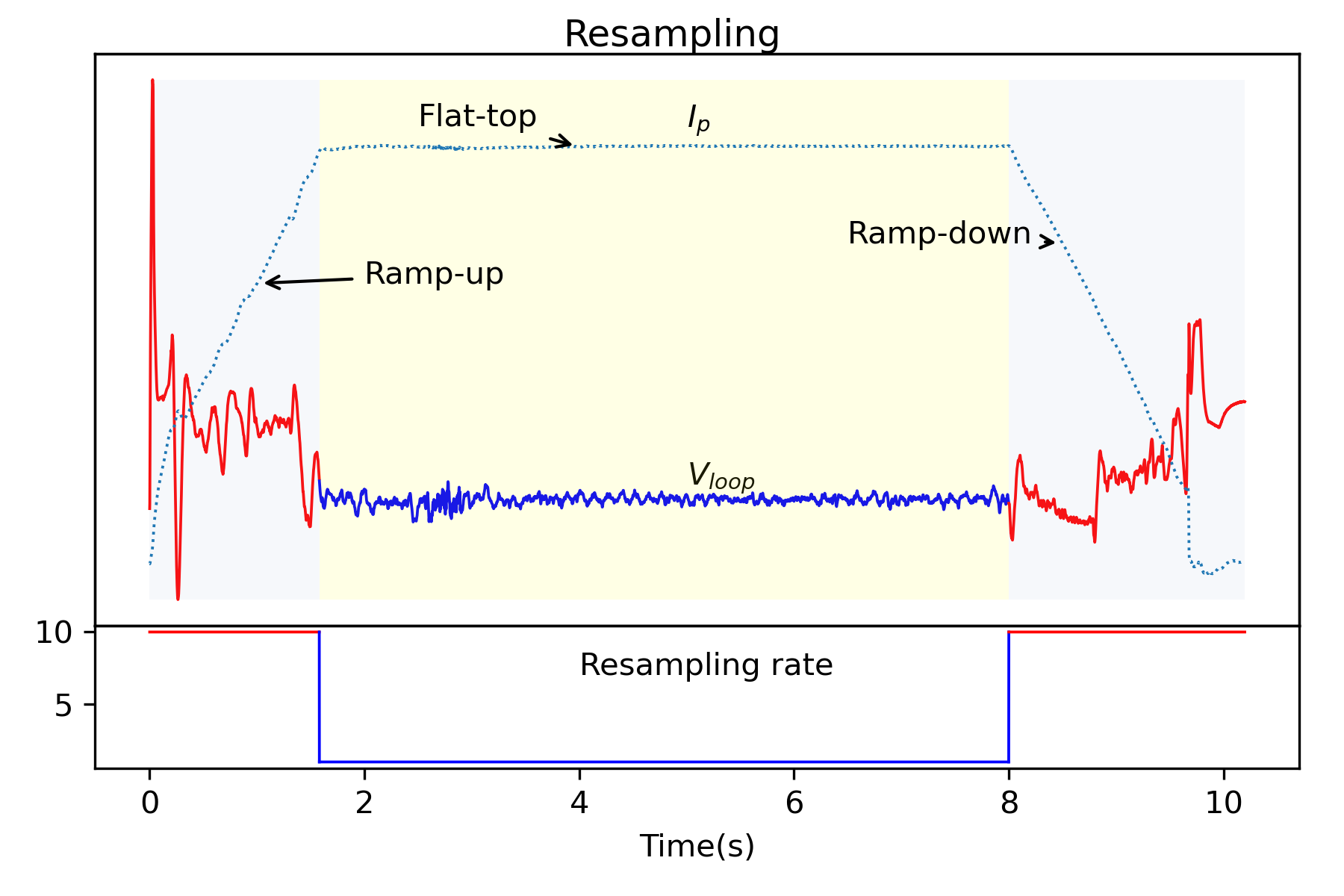
Figure 1: Schematic diagram of adaptive resampling. The higher resampling rate is used for segments that are of great interest to physicists or vary greatly and frequently.

Three signal channels are selected as outputs, and 65 channels are selected as inputs, and then resample according to the characteristics of the output signal to align the time points. In the next step, machine learning will be performed on these data.

3 Machine learning architecture

The data of tokamak diagnostic system are all temporal sequences, and different signal data have different characteristics. According to the temporal characteristics of the data of tokamak diagnostic system, the sequence to sequence (seq2seq) model [57] was chosen as the machine learning model for tokamak discharge modeling. Two methods of uniform resampling and adaptive resampling are adopted for different data characteristic.

Natural language processing (NLP) is more similar to the discharge modeling process than classification. NLP converts a natural language sequence into another natural language sequence. It is an important branch of machine learning, and the main algorithms are recurrent neural network (RNN), gated recurrent unit (GRU) and long-term short-term memory (LSTM), etc.

The encoder-decoder architecture [57] is a useful architecture in NLP, the architecture is partitioned into two parts, the encoder and the decoder. The encoder’s role is to encode the inputs into the state, which often contains several tensors. Then the state is passed into the decoder to generate the outputs. In this paper, LSTM was chosen as a fundamental component of the model. And stacked LSTM as an encoder-decoder machine learning model.

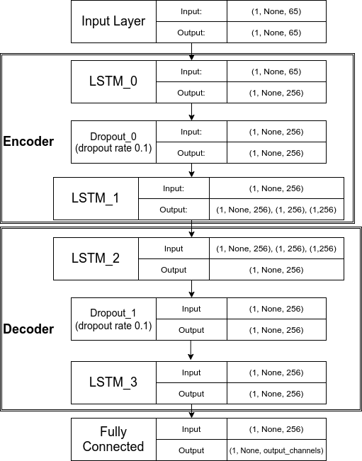
Figure 2: Architecture of our model. Where “None” represents different lengths of sequence because of different discharge shot duration time. “output_channels” is the number of output sequences.

As shown in figure 2, the machine learning model architecture used in this work is based on the sequence to sequence model (seq2seq) [57]. The first two LSTM layers (LSTM_0 and LSTM_1 in figure 2) and Dropout_0 can be considered as the encoder, and the last two LSTM layers (LSTM_2 and LSTM_3 in figure 2) and Dropout_1 can be regarded as the decoder. In this work, the encoder is to learn the high-level representation (cannot be displayed directly) of input signals (tab 1 input signals). The last hidden state of the encoder is used to initialize the hidden state of the decoder. The decoder plays the role of decoding the information of the encoder. Encoder-decoder is built as an end-to-end model, it can learn sequence information directly without manually extracting features.

In terms of components, the main component of our architecture is long short-term memory (LSTM) [58], because the LSTM can use trainable parameters to balance long-term and short-term dependencies. This feature is suitable for tokamak sequence data, tokamak discharge response is always strongly related to short-term input changes but it is also affected by long-term input changes (e.g. $W_{mhd}$ hardly changes fast, this property can be regarded as a short-term dependence. However, the impact of other factors on energy storage is cumulative. This property can be seen as long-term dependence.). The dropout layer is a common trick to prevent over-fitting. The final component is the fully connected layer to match the high-dimensional decoder output with the real target dimension.

When considering the specific mathematical principles of the model, the encoder hidden states $h_{t}$ are computed using this formula:

$$h_{t}=f(W^{(h_{lstm0}\delta_{dropout0}h_{lstm1})}h_{t-1}+W^{(hx)}x_{t}),$$ (1)

where $h_{lstm0}$, $h_{lstm1}$ are the hidden state of LSTM _0 and LSTM_1 in figure 2, $\delta_{dropout0}$ is the dropout rate in Dropout_0 in fig 2, $W$ and $W^{hx}$ are the appropriate weights to the previously hidden state $h_{t-1}$ and the input vector $x_{t}$. $\delta_{dropout0}\sim Bernoulli(p)$. This means $\delta_{dropout0}$ is equal to 1 with probability $p$ and 0 otherwise, we let $p=0.9$ for all experiment. Dropout_0 means that not all hidden states of LSTM_0 can be transferred to LSTM_1.

The encoder vector is the final hidden state produced from the encoder part of the model. It is calculated using the formula above. This vector aims to encapsulate the information for all input elements to help the decoder make accurate predictions. It acts as the initial hidden state of the decoder part of the model.

In decoder a stack of two LSTM units where each predicts an output $y_{t}$ at a time step $t$. Each LSTM unit accepts a hidden state from the previous unit and produces and output as well as its hidden state. In the modeling of tokamak discharge, The output sequence is a collection of all time steps from the $y$. Any hidden state $h_{t}$ is computed using the formula:

$$h_{t}=f(W^{(h_{lstm2}\delta_{dropout1}h_{lstm3})}h_{t-1}),$$ (2)

where $h_{lstm2,}h_{lstm3}$ are the hidden state of LSTM_2 and LSTM_3 in figure 2. $\delta_{dropout1}$ is the dropout rate in Dropout_1 in fig 2, $\delta_{dropout1}\sim Bernoulli(0.9)$. $W$ is the appropriate weights to the previously hidden state $h_{t-1}$. The process of data flowing in the decoder is similar to the encoder, but the initial states of $h_{lstm2}$ is equal to the last states of $h_{lstm1}$. As formula above, we are just using the previous hidden state to compute the next one. The output $y_{t}$ at time step t is computed using the formula:

$$y_{t}=activation(W^{D}h_{t}).$$ (3)

The model calculates the outputs using the hidden state at the current time step together with the respective weight $W^{D}$ of the fully connected layer as shown in figure 2 . The fully connected layer is used to determine the final outputs. The activation function is a linear function.

4 Training

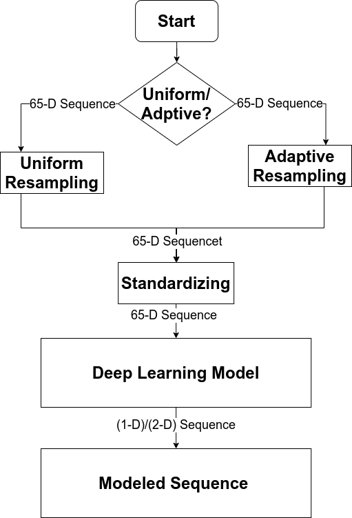
Figure 3: Workflow of training. The resampling method is determined according to the time characteristics of the output signal.

The form of the resampling function is determined according to the time characteristics of the output signal waveform. The output signals with the same sampling function are grouped together. The input signals are resampled using the same sampling function as the output signal set to ensure that all data points follow the same time axis. In this section, model training and data processing will be introduced in detail. The training of the model (see figure 3) can be divided into five steps as follows:

1. Obtaining the data of 68 channels (include input and output signals as shown in table 1) of the selected signals from the EAST source database.

2. Using different resampling methods base on the time characteristics of the output signal that would be modeled.

3. Standardizing the data with z-scores.

4. Data fed into the deep learning model for training.

5. Using the loss between model output and real experimental output as backing propagation metric and then update parameters for the training model.

The dataset is selected from EAST campaign 2016-2018, discharge shot number in the range #70000-80000 [53, 59, 55]. A total 3476 normal shots are selected and divide the data into a training set, a validation set, and a test set (training set: validation set: test set = 6: 2: 2). The normal shot means that no disruption occurred during this discharge, the flat top lasts more than two seconds, and the key signals (i.e., model output signals, magnetic field, and plasma current $I_{p}$) are complete. If there is no certain magnetic field configuration, plasma is impossible to be constrained and without completed $I_{p}$ or model output signals data there is no meaning for tokamak discharge experiment or this model. The sampling of the signal starts from $t=0s$ and continues to the end of the discharge ( typical EAST normal discharge time is five to eight seconds).

The shuffling method is a common improved generalization technique [60] used in an entire data set. However, in this work, the method is not used in the entire data set. In order to prevent data leakage caused by multiple adjacent discharge experimental shots with similar parameters, the entire data set is divided into training set, validation set and test set according to the experimental shot order. The phenomenon of adjacent discharge experimental shots with similar parameters is very common in tokamak discharge experiments. For generalization reasons, it is also necessary to shuffle shot order in the training set. For example, there are ten normal discharge shots in the original data set. For example, there are ten normal discharge shots in original data sets. The shot numbers of ten normal discharge shots are 1-10. the training set is shuffle(1-6) (maybe one order is 1,4,6,5,2,3), validation set is shuffle(7-8), and testing set is shuffle(9-10). Inner a single normal shot discharge sequence will keep strict time order.

When all source data was obtained the z-scores [61] will be applied for standardization. And then all the preprocessed data will be input to the deep learning model for training. In statistics, the z-score is the number of standard deviations by which the value of a raw score (i.e., an observed value or data point) is above or below the mean value of what is being observed or measured. Raw scores above the mean have positive standard scores, while those below the mean have negative standard scores. z-score is calculated by $z=(x-\mu\text{)/$\sigma$}$ where $\mu$ is the mean of the population. $\sigma$ is the standard deviation of the population.

The deep learning model uses an end-to-end training was executed on 8x Nvidia P100 GPUs with Keras [62] and TensorFlow [63] in the Centos7 system in local computing cluster and remote computing cluster. The training of the deep learning model starts with kernel initializer is glorot uniform initialization [64], the recurrent initializer is orthogonal [65], bias initializer is zeros, and optimizer is Adadelta [66] for solving gradient explosion. The model trains about twelve days, 40 epochs. Then use callbacks and checkpoints to choose the best performing model in $W_{mhd}$ and $n_{e}$ modeling best epoch is fifteen, while $V_{loop}$ modeling best epoch is seven. In per epoch, all the data in the training set will be put into the model for one time.

The training of our model is executed several times. Many of these trials are considered as failed (e.g. divergence in training, poor performance on the test set, etc) because of unsuitable hyper-parameters. In the process of training our model, multiple sets of hyperparameter are tried. Determine the best hyperparameter set by performance in the validation set. Finally, the best hyper-parameters were found by and shown in table 4.

Table 2: Hyperparameters in this model

Hyperparameter	Explanation	Best value
$\eta$	Learning rate	$5\times 10^{-3}$
$\gamma$

decay factor& 0.95 Loss function Loss function type Mean squared error (MSE) Optimizer Optimization scheme Adadelta Dropout Dropout probability 0.1 Epoch Epoch 15 and 7 dt Time step 0.001s Batch_size Batch size 1 LSTM type Type of LSTM CuDNNLSTM LSTM size Size of the hidden state of an LSTM unit. 256 $LSTM_{kernel}$ Initializer for the kernel of LSTM weights matrix Glorot uniform $LSTM_{recurrent}$ Initializer for the recurrent kernel of LSTM weights matrix Orthogonal Dense size Size of the Dense layer. 256 $Dense_{kernel}$ Initializer for the kernel of dense matrix Glorot uniform $Dense_{bias}$ Initializer for the bias vector Zeros $n_{encoder}$ Number of LSTMs stacked in encoder 2 $n_{decoder}$ Number of LSTMs stacked in decoder 2

5 Results

After the deep learning model had been trained, the model can model unseen data. As shown in figure 4, at the beginning of using the trained model, all data for 65 channel signals should be obtained. In this step, It is necessary to keep and select the same type of signal data in tokamak during training. The type of signal data includes processed data and raw data. And then aligning all the data on the time axis. The aligned data should be standardized by the same parameters of the training set. All the standardized data will be fed into the trained model and get the modeling sequence of diagnostic signals, In the final step, the trained model should be selected according to the diagnostic signal that you want to model.

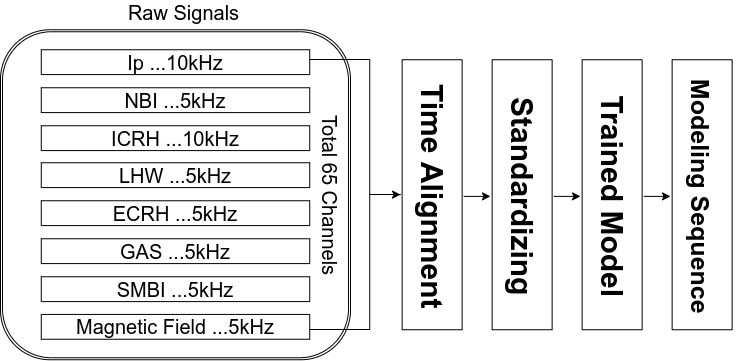
Figure 4: Using the trained model.

In this section, the results of modeling will be analyzed in detail, including representative modeling results and similarity distributions. In this work, the similarity is a quantitative measurement of the modeling results accuracy and is defined as follows:

$$S\left(\boldsymbol{x},\boldsymbol{y}\right)=\max\left(\frac{\Sigma(\boldsymbol{x}-\bar{\boldsymbol{x}})(\boldsymbol{y}-\bar{\boldsymbol{y}})}{\sqrt{\Sigma(\boldsymbol{x}-\bar{\boldsymbol{x}})^{2}\Sigma(\boldsymbol{y}-\bar{\boldsymbol{y}})^{2}}},0\right),$$ (4)

where $\boldsymbol{x}$ is experimental data, $\boldsymbol{y}$ is modeling result, $\bar{\boldsymbol{x}}$, $\bar{\boldsymbol{y}}$ are the means of the vector $\boldsymbol{x}$ and vector $\boldsymbol{y}$.

Two typical EAST normal discharge shots shot #77873 and #78461, are selected to check the accuracy of the model trained in this article. Figure 5(a) shows the modeling result for shot #77873, which has two LHW injections during discharge. Figure 5(b) shows the result for shot #78461, which has NBI, LHW, ICRF injection.

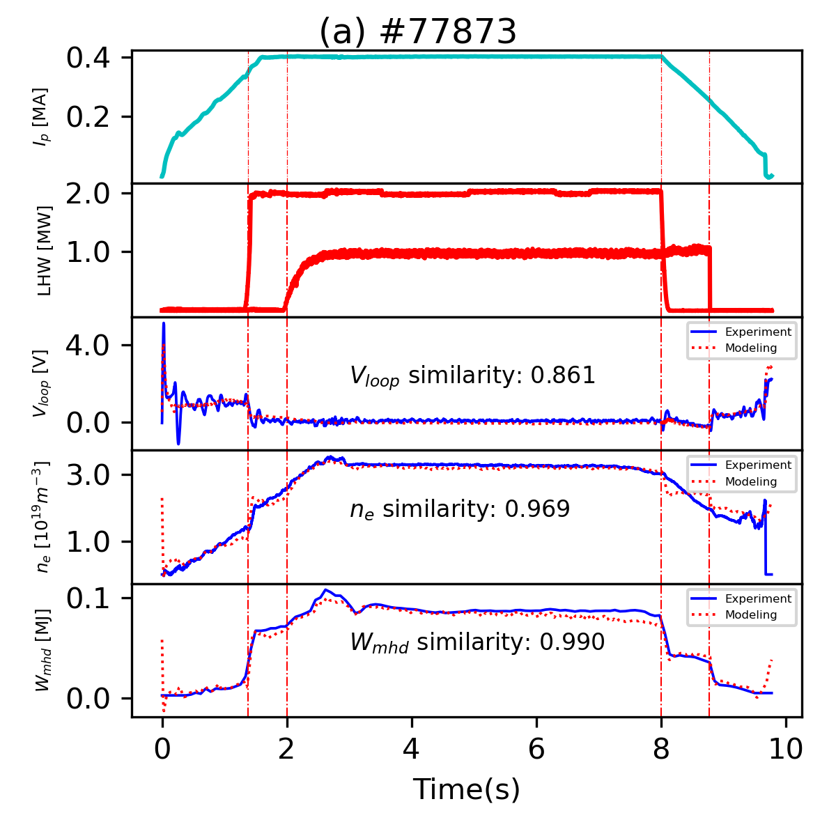
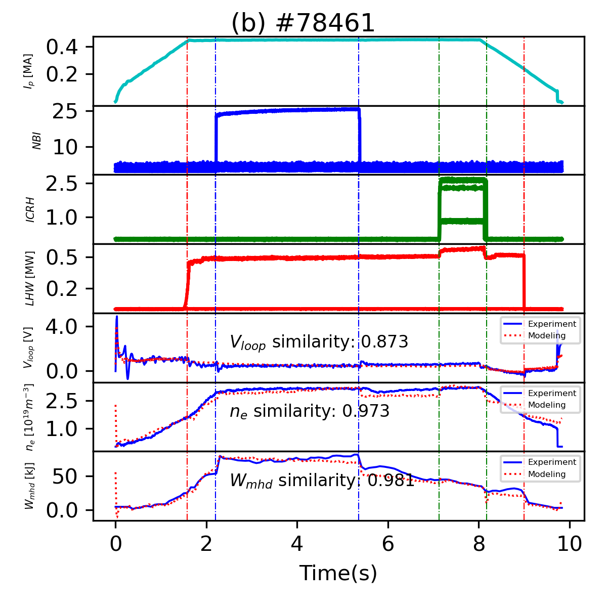
Figure 5: Comparison of modeling result and EAST experiment data, shot #77873 (a), and #78461 (b). NBI and ICRH are the raw data so the physical units are meaningless.

Experimental data and modeling results are displayed together in figure 5. The comparison shows that they are in good agreement in most regions of discharge, from ramp-up to ramp-down. The slope of the ramp-up and the amplitude of the flat-top are accurately reproduced by the model. The vertical dash-dot lines indicate the rising and falling edges of the external auxiliary system signal and the plasma response, which show the time accuracy of the model.

Compared with experimental signals, the modeling results are more sensitive to changes in external drives. For example, after the external drive is turned off, the experimental signal $n_{e}$ continues to decrease with a fixed slope, but the modeling results show a step-down. However, it will also cause the deviation of the modeling result and the experimental data when the external drive changes rapidly. How to adjust the sensitivity of the model is still an open question.

A test data set with 695 shots were used to quantitatively evaluate the reliability of the model. The statistical results of the similarity between model results and the experimental data are shown in figure 6.

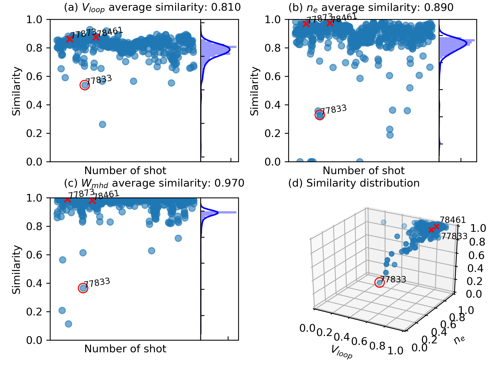
Figure 6: The similarity distribution and average similarity in the test set. show the similarity distributions of (a) $n_{e}$, (b) $V_{loop}$ , and (c) $W_{mhd}$, respectively. Figure (d) is a joint scatter plot of three parameters. If the similarity is less than 0, it is regarded as 0.

$W_{mhd}$ is the best performance parameters, with the similarity concentrated at more than 95%. In other words, $W_{mhd}$ can be considered to have been almost completely modeled under the normal discharge condition. The almost similarity of $n_{e}$ is greater than 85%. $V_{loop}$ is the worst performing parameter, but many of the errors are due to the plasma start-up pulse in the ramp-up segment and the plasma shutdown pulse in the ramp-down segment. However, $V_{loop}$ in the ramp-up and ramp-down sections is not the key factor for the operation of the experiment.

The joint distribution of the three parameters is shown in figure 6(d). Most shots are concentrated in a limited range, which reflect the consistency of the model on three target signals. It also shows that these shots belong to the same tokamak operating mode. In other words, those points far away from the center area indicate that the experiment is running in abnormal mode. We checked all deviation shots in test set, and all deviation are in abnormal conditions. For example, shot #77833 (as shown in figure 7) is a classical deviation caused by abnormal equipment conditions. This shot is used for cleaning device.

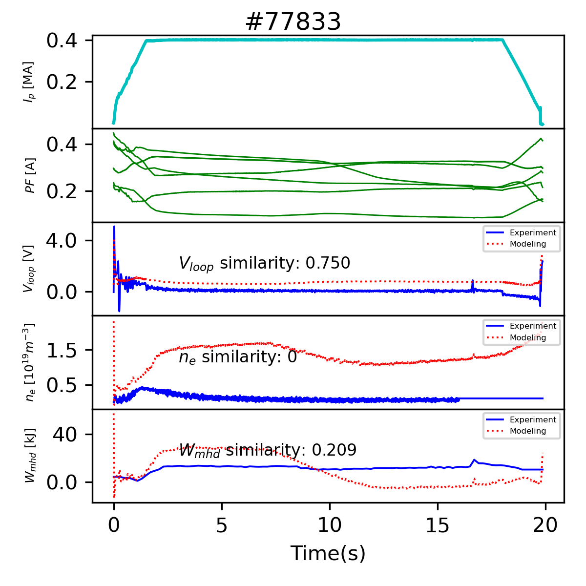
Figure 7: shot #77833 is a classical deviation caused by abnormal equipment conditions. Shot #77833 is used for cleaning device.

In terms of the similarity distribution of demonstrative parameters and representative discharge modeling results, this machine learning model application in tokamak discharge modeling is promising. $W_{mhd}$ can be regarded as almost completely reproduced under normal discharge shot. $n_{e}$ can be successfully modeled in most areas under the normal discharge condition. In normal discharge shot, the modeling results of $V_{loop}$ at ramp-down and flat-top phases are in good fitting with the experimental results.

6 Conclusion

In the present work, we showed the possibility of modeling the tokamak discharge process using experimental data-driven methods. A machine learning model based on the encoder-decoder was established and trained with the EAST experimental data set. This model can use the control signals (i.e. NBI, ICRH, etc.) to reproduce the normal discharge process (i.e. electron density $n_{e}$, store energy $W_{mhd}$ and loop voltage $V_{loop}$) without introducing physical models. Up to 95% similarity was achieved for $W_{mhd}$. Recent work of discharge modeling has focused on physical-driven “Integrated Modeling”. However, this work shows promising results for the modeling of tokamak discharge by using the data-driven methodology. This model can be easily extended to more physical quantities, and then a more comprehensive tokamak discharge model can be established.

Checking the physical goal of the experimental proposal is an important and complicated problem. This work provides a reference for the realization of physical goals under the normal discharge condition. Specifically, the model mainly checks whether an experimental proposal can be achieved under the normal discharge condition. Furthermore, if the experimental result deviates greatly from the result of our model, there may be two situations. one is that the experiment has some problems (as shown in figure 7); another is that a new discharge mode has appeared. The reason why a new discharge mode can be found is that this model only models discharge mode that has appeared in EAST normal discharges. Of note, if other discharge modes appear in the data, this model will appear chaotic output as if it were abnormal shots [67]. In general, chaotic model output means wrong input. For an experimental proposal, if the model gives a chaotic output, the input should be carefully checked by an experienced experimenter. If the input can be confirmed to be correct then it is likely to be a new discharge mode. Our model is not capable of fully accurate to recognize unsuccessful sets of inputs.

Compared with the physical-driven method, the data-driven method can build models more efficiently. We also realize that there are many challenges before the practical application of this method. For example, the impact of model sensitivity on modeling results has been recognized. How to adjust the sensitivity of the model is still an open question. Cross-device modeling is more important for devices under design and construction such as ITER and CFETR. Introducing device configuration parameters and performing transfer learning is a feasible solution to this problem. Our next step is to model the time evolution of the one-dimensional profile and the two-dimensional magnetic surface.

References

- [1] Gloria L Falchetto, David Coster, Rui Coelho, B D Scott, Lorenzo Figini, Denis Kalupin, Eric Nardon, Silvana Nowak, Luis Lemos Alves, and Jean-François Artaud. The European Integrated Tokamak Modelling (ITM) effort: achievements and first physics results. Nuclear Fusion, 54(4):43018, 2014.
- [2] R V Budny, R Andre, G Bateman, F Halpern, C E Kessel, A Kritz, and D McCune. Predictions of {H}-mode performance in {ITER}. Nuclear Fusion, 48(7):75005, 2008.
- [3] C E Kessel, R E Bell, M G Bell, D A Gates, S M Kaye, B P LeBlanc, J E Menard, C K Phillips, E J Synakowski, G Taylor, R Wilson, R W Harvey, T K Mau, P M Ryan, and S A Sabbagh. Long pulse high performance plasma scenario development for the {National} {Spherical} {Torus} {Experiment}. Physics of Plasmas, 13(5), 2006.
- [4] J F Artaud, V Basiuk, F Imbeaux, M Schneider, J Garcia, G Giruzzi, P Huynh, T Aniel, F Albajar, J M Ané, A Bécoulet, C Bourdelle, A Casati, L Colas, J Decker, R Dumont, L G Eriksson, X Garbet, R Guirlet, P Hertout, G T Hoang, W Houlberg, G Huysmans, E Joffrin, S H Kim, F Köchl, J Lister, X Litaudon, P Maget, R Masset, B Pégourié, Y Peysson, P Thomas, E Tsitrone, and F Turco. The {CRONOS} suite of codes for integrated tokamak modelling. Nuclear Fusion, 50(4):43001, 2010.
- [5] Michele Romanelli, Gerard Corrigan, Vassili Parail, Sven Wiesen, Roberto Ambrosino, Paula Da Silva Aresta Belo, Luca Garzotti, Derek Harting, Florian Köchl, Tuomas Koskela, Laura Lauro-Taroni, Chiara Marchetto, Massimiliano Mattei, Elina Militello-Asp, Maria Filomena Ferreira Nave, Stanislas Pamela, Antti Salmi, Pär Strand, and Gabor Szepesi. {JINTRAC}: {A} system of codes for integrated simulation of {Tokamak} scenarios. Plasma and Fusion Research, 9(SPECIALISSUE.2):1–4, 2014.
- [6] J. F. Artaud, F. Imbeaux, J. Garcia, G. Giruzzi, T. Aniel, V. Basiuk, A. Bécoulet, C. Bourdelle, Y. Buravand, J. Decker, R. Dumont, L. G. Eriksson, X. Garbet, R. Guirlet, G. T. Hoang, P. Huynh, E. Joffrin, X. Litaudon, P. Maget, D. Moreau, R. Nouailletas, B. Pégourié, Y. Peysson, M. Schneider, and J. Urban. Metis: A fast integrated tokamak modelling tool for scenario design. Nuclear Fusion, 58(10), 2018.
- [7] G V Pereverzev, P N Yushmanov, and Eta. {ASTRA}–{Automated} {System} for {Transport} {Analysis} in a {Tokamak}. Technical Report IPP 5/98, Max-Planck-Institut für Plasmaphysik, 1991.
- [8] N Hayashi and JET Team. Advanced tokamak research with integrated modeling in {JT}-60 {Upgrade}. Physics of Plasmas, 17(5), 2010.
- [9] O. Meneghini, S. P. Smith, L. L. Lao, O. Izacard, Q. Ren, J. M. Park, J. Candy, Z. Wang, C. J. Luna, V. A. Izzo, B. A. Grierson, P. B. Snyder, C. Holland, J. Penna, G. Lu, P. Raum, A. McCubbin, D. M. Orlov, E. A. Belli, N. M. Ferraro, R. Prater, T. H. Osborne, A. D. Turnbull, and G. M. Staebler. Integrated modeling applications for tokamak experiments with OMFIT. Nuclear Fusion, 55(8):83008, 2015.
- [10] Paul Bonoli, Lois Curfman McInnes, C Sovinec, D Brennan, T Rognlien, P Snyder, J Candy, C Kessel, J Hittinger, and L Chacon. Report of the Workshop on Integrated Simulations for Magnetic Fusion Energy Sciences. Technical report, 2015.
- [11] A Sengupta and P Ranjan. Forecasting disruptions in the ADITYA tokamak using neural networks. Nucl. Fusion, 40(12):1993, 2000.
- [12] A. Sengupta and P. Ranjan. Prediction of density limit disruption boundaries from diagnostic signals using neural networks. Nuclear Fusion, 41(5):487–501, 2001.
- [13] C. Rea, R. S. Granetz, K. Montes, R. A. Tinguely, N. Eidietis, J. M. Hanson, and B. Sammuli. Disruption prediction investigations using Machine Learning tools on DIII-D and Alcator C-Mod. Plasma Physics and Controlled Fusion, 60(8), 2018.
- [14] R A Tinguely, K J Montes, C Rea, R Sweeney, and R S Granetz. An application of survival analysis to disruption prediction via Random Forests. Plasma Physics and Controlled Fusion, 61(9):095009, 2019.
- [15] K.J. Montes, C. Rea, R.S. Granetz, R.A. Tinguely, N. Eidietis, O.M. Meneghini, D.L. Chen, B. Shen, B.J. Xiao, K. Erickson, and M.D. Boyer. Machine learning for disruption warnings on Alcator C-Mod, DIII-D, and EAST. Nuclear Fusion, 59(9):096015, 2019.
- [16] J.X. X Zhu, R.S. S Granetz, K. Montes, C. Rea, K. Montes, R.S. S Granetz, R Sweeney, and R A Tinguely. Hybrid deep learning architecture for general disruption prediction across tokamaks. arXiv preprint arXiv:2007.01401, pages 1–14, 2020.
- [17] Bihao Guo, Biao Shen, Dalong Chen, Cristina Rea, Robert Granetz, Yao Huang, Long Zeng, Heng Zhang, Jinping Qian, Youwen Sun, and Bingjia Xiao. Disruption prediction using a full convolutional neural network on EAST. Plasma Physics and Controlled Fusion, 2020.
- [18] Cristina Rea and Robert S. Granetz. Exploratory machine learning studies for disruption prediction using large databases on DIII-D. Fusion Science and Technology, 74(1-2):89–100, 2018.
- [19] D Wroblewski, G. L. Jahns, J. A. Leuer, D. Wróblewski, G. L. Jahns, and J. A. Leuer. Tokamak disruption alarm based on a neural network model of the high- limit. Nuclear Fusion, 37(6):725–741, 1997.
- [20] C. Rea, K.J. J Montes, K.G. G Erickson, R.S. S Granetz, and R.A. A Tinguely. A real-time machine learning-based disruption predictor in DIII-D. Nuclear Fusion, 59(9):096016, sep 2019.
- [21] P C De Vries, M F Johnson, B Alper, P Buratti, T C Hender, H R Koslowski, V Riccardo, and JET-EFDA Contributors. Survey of disruption causes at JET. Nuclear Fusion, 51(5):53018, 2011.
- [22] Jesús Vega, Sebastián Dormido-Canto, Juan M López, Andrea Murari, Jesús M Ramírez, Raúl Moreno, Mariano Ruiz, Diogo Alves, Robert Felton, JET-EFDA Contributors, and Fusion Engineering. Results of the JET real-time disruption predictor in the ITER-like wall campaigns. Fusion Engineering and Design, 88(6-8):1228–1231, 2013.
- [23] Barbara Cannas, Alessandra Fanni, A Murari, Alessandro Pau, Giuliana Sias, and J E T EFDA Contributors. Overview of manifold learning techniques for the investigation of disruptions on JET. Plasma Physics and Controlled Fusion, 56(11):114005, 2014.
- [24] G A Rattá, J Vega, and A Murari. Simulation and real-time replacement of missing plasma signals for disruption prediction: an implementation with APODIS. Plasma Physics and Controlled Fusion, 56(11):114004, 2014.
- [25] A. Murari, M. Lungaroni, E. Peluso, P. Gaudio, J. Vega, S. Dormido-Canto, M. Baruzzo, and M. Gelfusa. Adaptive predictors based on probabilistic SVM for real time disruption mitigation on JET. Nuclear Fusion, 58(5):56002, 2018.
- [26] A. Pau, A. Fanni, B. Cannas, S. Carcangiu, G. Pisano, G. Sias, P. Sparapani, M. Baruzzo, A. Murari, F. Rimini, M. Tsalas, P. C. De Vries, and Pau A Et al. A first analysis of JET plasma profile-based indicators for disruption prediction and avoidance. IEEE Trans. Plasma Sci., 46(7):2691, 2018.
- [27] R M Churchill, Princeton Plasma, General Atomics, and San Diego. Deep convolutional neural networks for multi-scale time-series classification and application to disruption prediction in fusion devices arXiv : 1911 . 00149v2 [ physics . plasm-ph ] 21 Nov 2019. (NeurIPS):1–6, 2019.
- [28] Julian Kates-Harbeck, Alexey Svyatkovskiy, and William Tang. Predicting disruptive instabilities in controlled fusion plasmas through deep learning. Nature, 568(7753):526–531, 2019.
- [29] Barbara Cannas, Alessandra Fanni, E Marongiu, and P Sonato. Disruption forecasting at JET using neural networks. Nuclear fusion, 44(1):68, 2003.
- [30] C G Windsor, G Pautasso, C Tichmann, R J Buttery, T C Hender, and J E T EFDA Contributors. A cross-tokamak neural network disruption predictor for the JET and ASDEX Upgrade tokamaks. Nuclear fusion, 45(5):337, 2005.
- [31] Barbara Cannas, Alessandra Fanni, E Marongiu, P Sonato, Marongiu E Cannas B Fanni A, and Sonato P. Disruption forecasting at JET using neural networks. Nucl. Fusion, 44(1):68, 2004.
- [32] Barbara Cannas, Rita Sabrina Delogu, ALESSANDRA Fanni, P Sonato, MARIA KATIUSCIA Zedda, and JET-EFDA Contributors. Support vector machines for disruption prediction and novelty detection at JET. Fusion engineering and design, 82(5-14):1124, 2007.
- [33] A Murari, G Vagliasindi, P Arena, L Fortuna, O Barana, M Johnson, and JET-EFDA Contributors. Prototype of an adaptive disruption predictor for JET based on fuzzy logic and regression trees. Nuclear Fusion, 48(3):35010, 2008.
- [34] A. Murari, J. Vega, G. A. Ratt, G. Vagliasindi, M. F. Johnson, and S. H. Hong. Unbiased and non-supervised learning methods for disruption prediction at JET. Nuclear Fusion, 49(5), 2009.
- [35] G. A. Ratt, J. Vega, A. Murari, G. Vagliasindi, M. F. Johnson, and P. C. De Vries. An advanced disruption predictor for JET tested in a simulated real-time environment. Nuclear Fusion, 50(2):25005, 2010.
- [36] D R Ferreira, P J Carvalho, and H Fernandes. Deep Learning for Plasma Tomography and Disruption Prediction From Bolometer Data. IEEE Transactions on Plasma Science, 48(1):36–45, jan 2020.
- [37] Barbara Cannas, Alessandra Fanni, G Pautasso, G Sias, and P Sonato. An adaptive real-time disruption predictor for ASDEX Upgrade. Nuclear Fusion, 50(7):75004, 2010.
- [38] G Pautasso, Ch Tichmann, S Egorov, T Zehetbauer, O Gruber, M Maraschek, K-F Mast, V Mertens, I Perchermeier, and G Raupp. On-line prediction and mitigation of disruptions in ASDEX Upgrade. Nuclear Fusion, 42(1):100, 2002.
- [39] R. Aledda, B. Cannas, A. Fanni, A. Pau, G. Sias, Fanni A Pau A Aledda R Cannas B, and Sias G. Improvements in disruption prediction at ASDEX Upgrade. Fusion Eng. Des., 96–97:698, 2015.
- [40] R Yoshino and Yoshino R. Neural-net disruption predictor in JT-60U. Nucl. Fusion, 43(12):1771, 2003.
- [41] R Yoshino. Neural-net predictor for beta limit disruptions in JT-60U. Nuclear fusion, 45(11):1232, 2005.
- [42] Zongyu Yang, Fan Xia, Xianming Song, Zhe Gao, Yao Huang, and Shuo Wang. A disruption predictor based on a 1.5-dimensional convolutional neural network in {HL}-{2A}. Nuclear Fusion, 60(1):16017, 2020.
- [43] Bin Yang, Zhenxing Liu, Xianmin Song, Xiangwen Li, and Yan Li. Modeling of the HL-2A plasma vertical displacement control system based on deep learning and its controller design. Plasma Physics and Controlled Fusion, 62(7):075004, July 2020.
- [44] S P Gerhardt, D S Darrow, R E Bell, B P LeBlanc, J E Menard, D Mueller, A L Roquemore, S A Sabbagh, and H Yuh. Detection of disruptions in the high- spherical torus NSTX. Nuclear Fusion, 53(6):63021, 2013.
- [45] J. Text Team, W. Zheng, F. R. Hu, M. Zhang, Z. Y. Chen, X. Q. Zhao, X. L. Wang, P. Shi, X. L. Q. Zhang, X. L. Q. Zhang, Y. N. Zhou, Y. N. Wei, and Y. Pan. Hybrid neural network for density limit disruption prediction and avoidance on J-TEXT tokamak. Nuclear Fusion, 58(5):56016, mar 2018.
- [46] Huang D W Tong R H Yan W Wei Y N Ma T K Zhang M Wang S Y Chen Z Y, Zhuang G, S. Y. Wang, Z. Y. Chen, D. W. Huang, R. H. Tong, W. Yan, Y. N. Wei, T. K. Ma, M. Zhang, and G. Zhuang. Prediction of density limit disruptions on the j-TEXT tokamak. Plasma Phys. Control. Fusion, 58(5), apr 2016.
- [47] M. Honda and E. Narita. Machine-learning assisted steady-state profile predictions using global optimization techniques. Physics of Plasmas, 26(10), 2019.
- [48] O. Meneghini, S. P. Smith, P. B. Snyder, G. M. Staebler, J. Candy, E. Belli, L. Lao, M. Kostuk, T. Luce, T. Luda, J. M. Park, and F. Poli. Self-consistent core-pedestal transport simulations with neural network accelerated models. Nuclear Fusion, 57(8):86034, 2017.
- [49] O Meneghini, Garud Snoep, Brendan C Lyons, Joseph McClenaghan, Chieko Sarah Imai, Brian A Grierson, Sterling P Smith, Gary M Staebler, Philip B Snyder, Jeff Candy, Emily A Belli, L L Lao, Jin Myung Park, Jonathan Citrin, Teobaldo Luda di Cortemiglia, Arsène Stéphane Tema Biwole, and Saskia Mordijck. Neural-network accelerated coupled core-pedestal simulations with self-consistent transport of impurities and compatible with ITER IMAS. Nuclear Fusion, 2020.
- [50] Alex Graves. Generating sequences with recurrent neural networks. arXiv preprint arXiv:1308.0850, 2013.
- [51] Zachary C. Lipton, John Berkowitz, and Charles Elkan. A Critical Review of Recurrent Neural Networks for Sequence Learning. pages 1–38, 2015.
- [52] Hassan Ismail Fawaz, Germain Forestier, Jonathan Weber, Lhassane Idoumghar, and Pierre Alain Muller. Deep learning for time series classification: a review. Data Mining and Knowledge Discovery, 33(4):917–963, 2019.
- [53] Baonian Wan, Jiangang Li, Houyang Guo, Yunfeng Liang, Guosheng Xu, Liang Wang, and Xianzu Gong. Advances in H-mode physics for long-pulse operation on EAST. Nuclear Fusion, 55(10):104015, 2015.
- [54] B. N. Wan, Y. Liang, X. Z. Gong, N. Xiang, G. S. Xu, Y. Sun, L. Wang, J. P. Qian, H. Q. Liu, L. Zeng, L. Zhang, X. J. Zhang, B. J. Ding, Q. Zang, B. Lyu, A. M. Garofalo, A. Ekedahl, M. H. Li, F. Ding, S. Y. Ding, H. F. Du, D. F. Kong, Y. Yu, Y. Yang, Z. P. Luo, J. Huang, T. Zhang, Y. Zhang, G. Q. Li, and T. Y. Xia. Recent advances in EAST physics experiments in support of steady-state operation for ITER and CFETR. Nuclear Fusion, 59(11):1–12, 2019.
- [55] Jiangang Li, Baonian Wan, EAST Team, and Int Collaborators. Recent progress in RF heating and long-pulse experiments on EAST. NUCLEAR FUSION, 51(9, SI), SEP 2011.
- [56] Feng Wang, Yueting Wang, Ying Chen, Shi Li, and Fei Yang. Study of web-based management for EAST MDSplus data system. Fusion Engineering and Design, 129:88–93, April 2018.
- [57] Ilya Sutskever, Oriol Vinyals, and Quoc V. Le. Sequence to sequence learning with neural networks. Advances in Neural Information Processing Systems, 4(January):3104–3112, 2014.
- [58] Sepp Hochreiter and Jürgen Schmidhuber. Long short-term memory. Neural computation, 9(8):1735–1780, 1997.
- [59] Baonian Wan, Jiangang Li, Houyang Guo, Yunfeng Liang, Guosheng Xu, and Xianzhu Gong. Progress of long pulse and H-mode experiments in EAST. Nuclear Fusion, 53(10), 2013.
- [60] Kenji Kawaguchi Leslie Pack Kaelbling and Yoshua Bengio. Generalization in Deep Learning. Technical report.
- [61] Dennis Zill, Warren S Wright, and Michael R Cullen. Advanced engineering mathematics. Jones & Bartlett Learning, 2011.
- [62] François Chollet and Others. Keras. https://keras.io, 2015.
- [63] Martn Abadi, Ashish Agarwal, Paul Barham, Eugene Brevdo, Zhifeng Chen, Craig Citro, Greg S Corrado, Andy Davis, Jeffrey Dean, Matthieu Devin, et al. Tensorflow: Large-scale machine learning on heterogeneous distributed systems. arXiv preprint arXiv:1603.04467, 2016.
- [64] Xavier Glorot and Yoshua Bengio. Understanding the difficulty of training deep feedforward neural networks. In Journal of Machine Learning Research, volume 9, pages 249–256, 2010.
- [65] Andrew M. Saxe, James L. McClelland, and Surya Ganguli. Exact solutions to the nonlinear dynamics of learning in deep linear neural networks. arXiv preprint arXiv:1312.6120, 2013.
- [66] Matthew D. Zeiler. ADADELTA: An Adaptive Learning Rate Method. arXiv preprint arXiv:1212.5701, 2012.
- [67] Yann LeCun, Yoshua Bengio, and Geoffrey Hinton. Deep learning. NATURE, 521(7553):436–444, 2015.