HInet: Generating neutral hydrogen from dark matter with neural networks

Abstract

Upcoming 21cm surveys will map the spatial distribution of cosmic neutral hydrogen (HI) over very large cosmological volumes. In order to maximize the scientific return of these surveys, accurate theoretical predictions are needed. Hydrodynamic simulations currently are the most accurate tool to provide those predictions in the mildly to non-linear regime. Unfortunately, their computational cost is very high: tens of millions of CPU hours. We use convolutional neural networks to find the mapping between the spatial distribution of matter from N-body simulations and HI from the state-of-the-art hydrodynamic simulation IllustrisTNG. Our model performs better than the widely used theoretical model: Halo Occupation Distribution (HOD) for all statistical properties up to the non-linear scales $k\lesssim 1$ h/Mpc. Our method allows the generation of 21cm mocks over very big cosmological volumes with similar properties as hydrodynamic simulations.

1 Introduction

Different astronomical surveys have allowed us to quantify the amount and properties of several fundamental quantities like the age, geometry and expansion rate of the Universe, and the amount of dark matter and dark energy. Some of the largest surveys in the past have been spectroscopic surveys of galaxies, which have mapped the Universe at low redshifts. In future surveys, we want to observe the Universe at high-$z$ because the cosmic volume is larger and the theoretical predictions at high-$z$ are relatively easier as the density field is more linear.

The traditional technique of getting spectra of individual galaxies becomes harder to apply at high-$z$ as the galaxies become fainter and sparser. One of the most promising alternative techniques to observe the high-$z$ Universe is Intensity Mapping (IM) (Bharadwaj et al., 2001; Bharadwaj & Sethi, 2001; Chang et al., 2008; Peterson et al., 2009; Pullen et al., 2014) The advantage of IM over the traditional techniques is that it does not rely on resolving point sources but instead measures the emission from many unresolved galaxies tracing the cosmic web in redshift space.

In this paper we focus our attention on IM of the 21cm line from cosmic neutral hydrogen (hereafter Hi  ). It is worth noting that 21cm IM is not just restricted to the high-$z$ but is applicable over a wide range of redshifts ($z=0$ to $z\simeq 20$). 21cm surveys represent a different way to observe the Universe, and they enable new cross-correlations with surveys at other wavelengths, which are very effective to mitigate systematic effects. Besides traditional bounds on cosmological parameters (Bull et al., 2015; Villaescusa-Navarro et al., 2017), 21cm surveys can be used to improve our knowledge on the sum of neutrino masses (Villaescusa-Navarro et al., 2015a), warm DM (Carucci et al., 2015), modified gravity (Carucci et al., 2017), primordial non-Gaussianity (Karagiannis et al., 2019) and axion DM (Bauer et al., 2020), among many other things.

In this work, we focus our attention on the the post-reionization regime ($z<6$) of 21 cm IM, for which various radio surveys are planned or are already collecting data: Canadian Hydrogen Intensity Mapping Experiment (CHIME) Giant Meterwave Radio Telescope (GMRT) , HIRAX (The Hydrogen Intensity and Real-time Analysis eXperiment) , TIANLAI , Five-hundred-meter Aperture Spherical Telescope (FAST) , ASKAP , MeerKAT , PUMA , SKA (The Square Kilometer Array) .

One of the major aims of these surveys is to accurately constrain the value of the cosmological parameters. In order to achieve this, accurate theoretical predictions are needed to extract the cosmological information from the collected data. In the linear regime, these predictions are easy to obtain from analytical models and are accurate. However, there is a large amount of cosmological information that lies beyond the linear scales, particularly at low-$z$. In this regime, one avenue to obtain such accurate predictions is from hydrodynamic simulations.

Current state-of-the-art hydrodynamic simulations have a very high computational cost and they simulate a limited cosmological volume. For example, simulating the $(75\,h^{-1}\,{\rm Mpc})^{3}$ IllustrisTNG box required 18 million CPU hours (Nelson et al., 2019; Pillepich et al., 2018; Weinberger et al., 2017). In order to make robust predictions for upcoming astronomical surveys we need to simulate much larger cosmological volumes, of the order of tens to hundreds of $(\textup{Gpc/h})^{3}$ (Modi et al., 2019a). Such large mock simulations would help us in various ways: 1) to study the effects of various observational systematics on the statistical properties of the tracers, 2) to obtain theoretical predictions for different cosmologies, 3) to determine which summary statistics are the most appropriate to constrain the value of different cosmological parameters, 4) to quantify the cosmic variance in the surveys (i.e, to compute the covariance matrix). One way to simulate large Hi  volumes is to first generate dark matter (DM) fields using the relatively less expensive DM-only simulations. We then need quick and reliable methods to ‘paint’ Hi  directly on the DM field. We now discuss some promising techniques in this regard.

1.1 Traditional emulation techniques

One the most popular theoretical techniques used to make mock baryonic simulations is called the Halo Occupation Distribution (HOD). HOD was first used to probabilistically model the number of galaxies residing in a host halo (Scoccimarro et al., 2001; Seljak, 2000; Peacock & Smith, 2000; Berlind & Weinberg, 2002). The HOD technique assumes that the properties of various baryonic structures inside a halo are governed solely by the halo mass, and ignores all other halo properties. The HOD technique therefore assumes a simple parametric relation between the halo mass and the baryonic properties and uses hydrodynamical simulations (and observations, if available) to calibrate the parameters in this relation. Recent applications of the HOD technique to Hi  have been in initial field reconstruction and testing the UV background effect on Hi  maps (Modi et al., 2019a, b) based on the HOD model of Villaescusa-Navarro et al. (2018, hereafter VN18).

However, HOD ignores all environmental effects on the Hi  abundance and clustering. It is important to note that numerical simulations have shown that cosmological properties like the clustering of halos and galaxies are affected by properties other than halo mass like halo environment, halo concentration, spin and velocity anisotropy and others (Wechsler et al., 2006; Dalal et al., 2008; Paranjape et al., 2018; Hadzhiyska et al., 2020). This phenomenon referred to as assembly bias or secondary bias (Sheth & Tormen, 2004; Gao et al., 2005).

Other techniques can be used to make mock baryonic simulations, such as Subhalo Abundance Matching (SHAM) and semi-analytic models (SAM). SHAM involves assigning the highest Hi  mass to the most massive halos and vice versa but it relies on multiple assumptions like more massive baryonic structures are hosted by the most massive halos and a monotonic relation ,which is free of scatter, exists between masses of baryonic structures and halo masses. SAM, on the other hand, uses a set of simplified equations to model the key baryonic processes in the hydrodynamic simulations (for example, see Benson (2012)).

It is worth mentioning that, apart from using simulations, there are also proposed perturbative forward model techniques to evolve the tracer fields directly from linear initial conditions by using biasing schemes (Schmittfull et al., 2019; Modi et al., 2020) (or modeling tracer fields by combining biasing schemes and $N$-body simulations (Sinigaglia et al., 2020)).

1.2 Convolutional neural networks

Convolutional neural networks (CNNs) have been recently applied to numerous areas of physical research (Carleo et al., 2019) and have a lot of potential applications to cosmology (Ntampaka et al., 2019; Ravanbakhsh et al., 2017; Zamudio-Fernandez et al., 2019; Zhang et al., 2019; He et al., 2019; Giusarma et al., 2019; Modi et al., 2018; Kodi Ramanah et al., 2020). An important property of CNNs which makes them useful for cosmological applications is that they are translationally equivariant. In this paper, we use a modified version of a neural network architecture called U-Net to generate mock 3D Hi  fields from a given DM field. Although we focus on Hi  in the post-reionization regime in this paper, it is worth mentioning some of the recent work on using neural networks to study the Hi  field during the epoch of reionization (Shimabukuro & Semelin, 2017; Gillet et al., 2019; Chardin et al., 2019; List & Lewis, 2020; Kwon et al., 2020; Mangena et al., 2020; Hassan et al., 2020; Villanueva-Domingo & Villaescusa-Navarro, 2020).

Let us now briefly highlight some of the advantages of neural networks over the above traditional approaches. The HOD formalism typically assumes that the spatial Hi  density $\rho_{\rm HI}({\bf x})$ at a particular point inside a halo only depends on the mass of the halo and the distance to its center:

$$\rho_{\textup{HI}}({\bf x})=f(M_{\rm halo},|{\bf x}-{\bf x}_{\rm center}|)$$ (1)

However, VN18 showed that including only the halo mass is not enough for precisely modeling the clustering of the Hi  field. A more general model for Hi  field should also include the information on the environment of the halo and can be roughly intuited as

$$\rho_{\rm HI}({\bf x})=g(\rho_{\rm m}({\bf x}),\rho_{\rm m}({\bf x}^{\prime}))$$ (2)

where $\rho_{\rm m}({\bf x}^{\prime})$ is the matter density at points in the neighborhood of ${\bf x}$. Neural networks are universal fitting functions (Hornik et al., 1989) and can be used to accurately approximate the function $g$ in Equation 2; this is the goal of our paper.

The paper is organized as follows. In Section 2, we briefly describe the hydrodynamical simulations that we have used. We then present the specific architecture of our machine learning model and the method used in Section 3. We discuss the parameters of our benchmark HOD model in Section 4. We present our results in Section 5. Finally, we discuss our results in Section 6 and conclude in Section 7.

2 Data

The data we use to train, validate and test our network is obtained from the TNG100-1 simulation produced by the IllustrisTNG collaboration (Pillepich et al., 2018). That simulation is one of the current state-of-the-art hydrodynamical simulations and includes a wide range of relevant physical effects, such as radiative cooling, star formation, metal enrichment, supernova and AGN feedback, and magnetic fields. In this work, we choose to model the Hi  field at low redshift: $z=1$; this is because modeling any baryonic field is more challenging at lower redshifts due the density fluctuations being relatively non-linear. We therefore expect our neural network method to perform even better at higher redshifts.

The side length of the simulated box is 75 h^-1 Mpc. We first compute the Hi  density field by assigning Hi  masses of gas cells to a grid of $2048^{3}$ cells using the cloud-in-cell (CIC) interpolation scheme. The spatial resolution of the DM and Hi  fields is therefore very high $\sim 35\,h^{-1}\,{\rm kpc}$. TNG provides both the hydrodynamical simulation output as well as the computationally cheaper dark matter only simulation (TNG100-1-DM), evolved from the same initial conditions. Our goal is to train a neural network such that it can produce the Hi  field from the DM only simulation. The network performs the mapping in 3D, at a fixed redshift.

2.1 Data preprocessing

The overdensity in the Hi  field, $\delta_{\textup{HI}}\,=\rho_{\rm HI}/\bar{\rho}_{\rm HI}-1$, varies in the TNG100-1 simulation across $\sim$9 orders of magnitude. Because the resolution of the TNG100-1 simulation is much higher than the one expected from upcoming surveys, we smooth the Hi  data with a Top-Hat filter with a smoothing radius of 300 $h^{-1}{\rm kpc}$. This has a two-fold advantage: First, the grid resolution for the Hi  field is lowered to 140 $\,h^{-1}\,{\rm kpc}$, which reduces the size of the dataset. Second, the dynamical range over which the Hi  density field varies is reduced: $\delta_{\textup{HI}}\,$ varies over three orders of magnitude and this reduces the sparsity problem which we later discuss in section 3. Note that we did not change the resolution of the input DM field, in order to use as much information in the DM field as possible. Because the training of deep learning models is facilitated when the input data is in the $\mathcal{O}(1)$ range, we further perform the scaling:

$$\begin{split}\tilde{\delta}_{\textup{HI}}\,({\bf x})&\equiv\frac{1}{2}(1+\delta_{\textup{HI}}\,({\bf x}))^{0.2}\\ \tilde{\delta}_{\textup{DM}}({\bf x})&\equiv\frac{1}{5}(1+\delta_{\textup{DM}}({\bf x}))^{0.1}\,,\end{split}$$ (3)

where $\delta_{\textup{HI}}\,$ is the smoothed Hi  field. The above rescaling get both $\tilde{\delta}_{\textup{HI}}\,$ and $\tilde{\delta}_{\textup{DM}}$ to be in the nearly in the range [0, 3]. We used a power law instead of a logarithm because the power law distribution has a flatter tail for high values of $\delta_{\textup{HI}}\,$. We discuss why having a flatter tail is important in Section 3.2.

3 Methods

3.1 Choice of network architecture

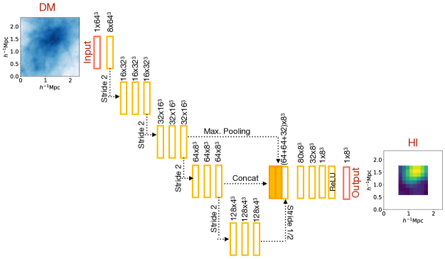
The deep neural network architecture used in this paper is inspired by the Deep Density Displacement Model (D³M) of He et al. (2019). D³M is the generalization of the standard U-Net which was first proposed by Ronneberger et al. (2015) for use in medical applications. Convolutional neural networks, like the U-Net, naturally provide properties which are relevant for our problem such as translational invariance. Variations of the D³M model have been used for large scale structure applications like learning galaxy modeling and neutrino effects in cosmology (Yip et al., 2019; Zhang et al., 2019; Giusarma et al., 2019). The network architecture we use in this work is shown in Figure 1, and further details are presented in Appendix A.

Figure 1: This scheme shows the architecture we use to find the mapping from dark matter to HI in 3D. Labels represent [number of channels $\times$ (number of voxels)³]. Further details can be found in Appendix A. Notice that the volume of the Hi  output is $1/8^{\textup{th}}$ of the input DM volume, which enables inclusion of some of the non-local (environmental) information to predict the Hi  field.

3.2 Challenge of data sparsity

Let us discuss an important challenge we face when working with HI data from simulations. The most relevant summary statistics for 21cm IM, e.g. the HI power spectrum or the HI PDF, are dominated by the voxels with the highest HI density. The reason for this is that 21cm IM is sensitive to the mass-weighted HI, rather than the volume-weighted HI of, e.g., the Ly$\alpha$ forest. Unfortunately, those dense voxels are rare in the simulation. For instance, there are $\sim 10^{5}$ halos with $M_{\textup{halo}}\geq 10^{10}h^{-1}M_{\odot}$ in our dataset, which translates in a very small subset ($\sim$1 in 10³) of voxels of our training sample having a non-negligible HI density (see the distribution of the voxel Hi  masses in Figure 7). Because of such sparsity in our data distribution, our model could easily achieve a high accuracy by predicting the low mass Hi  voxels, ignoring the high mass Hi  voxels; this makes our model harder to train.

Modeling the fields in Lagrangian space rather than Eulerian space can in principle reduce the sparsity problem. This is because in lagrangian space we use the displacement field, which is distributed over a larger region of space, as compared to the density field, which is largely concentrated inside the halo boundaries (He et al., 2019). However, modeling the Hi  field is not possible in lagrangian space because, unlike DM, the number of gas particles are not fixed in the simulation.

A similar sparsity challenge exists when predicting the galaxy positions from a 3D DM field. Some of the previous neural network based studies have tried to overcome this challenge by using a combination of two neural networks (two-phase model) (Zhang et al., 2019; Yip et al., 2019; Modi et al., 2018): the first phase predicts the halo/galaxy position and the second phase predicts the mass of the halo/ number of galaxies. However, Hi  , unlike galaxies, is scattered over a wide volume of the Universe, not just at the centers of large DM halos. Ignoring the low mass voxels would remove the Ly$\alpha$ forest from our data which is not ideal as the Ly$\alpha$ forest is a powerful cosmological probe by itself, and its contribution to the 21cm signal at high-redshift becomes more important (VN18).

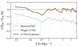
We therefore implement a different kind of two-phase model: the first (second) network is geared towards predicting the low mass (high mass) Hi  voxels. We have used the same U-Net architecture shown in Figure 1 for each of the two phases of our model. We provide further details of the two-phase model in Appendix A.

3.3 Training the network

As the memory of GPUs is limited, we split the 75$\,h^{-1}\,{\rm Mpc}$ TNG100 volume into smaller sub-boxes. We train the U-Net to predict Hi  boxes of side length $\sim$1.17 h^-1 Mpc and containing $8^{3}$ voxels using input DM boxes of side length $\sim$2.34 h^-1 Mpc and $64^{3}$ voxels. As illustrated in Figure 1, we want to predict the Hi  in the sub-box residing at the center of a larger DM input. The motivation of using the larger DM box is to account for environmental information for voxels near the boundaries of the HI volume.

We obtain $\sim 2.5\times 10^{5}$ non-overlapping Hi  sub-boxes when splitting the TNG100-1 volume. We divide these sub-boxes in three chunks: $\sim$ 60% of the sub-boxes are used for training the network, 12.5% for validation and 27.5% for testing the network. We have constructed the test set such that it comprises of all the sub-boxes which correspond to a larger box of side-length $\sim$ 48 $\,h^{-1}\,{\rm Mpc}$. The total number of trainable parameters in the U-Net shown in Figure 1 is $2.1\times 10^{7}$, which, although seems gigantic, can be optimized using the technique of automatic differentiation (gradient descent). The gradients are calculated based on the following loss function

$$\mathbb{L}=\sum_{i}^{\textup{Voxels}}(\tilde{\delta}^{\textup{pred}}_{i}-\tilde{\delta}^{\textup{Illustris}}_{i})^{2}\times\exp[(\tilde{\delta}^{\textup{Illustris}}_{i}-\beta)^{\alpha}]$$ (4)

where $\tilde{\delta}$ is the scaled Hi  density field from Eq. (3). Notice that our loss function is different from the traditional mean square error (MSE) loss; we use the additional hyperparameters $\alpha$ and $\beta$ to add more weight to the high mass voxels in order to alleviate the aforementioned sparsity problem. We find that $\alpha=2$ and $\beta=0.7$ give the best results. We provide further details on the training of the network in Appendix A. We have also made use of the techniques of data augmentation and imbalanced sampling to tackle the sparsity problem and we provide further details in Appendix A.3.

4 Benchmark model: Halo Occupation Distribution (HOD)

We will compare the results of our neural network against a benchmark model, that we describe in detail in this section.

There have been multiple recent attempts at developing a halo model for the abundance and spatial distribution of Hi  (Villaescusa-Navarro et al., 2014; Castorina & Villaescusa-Navarro, 2017; Villaescusa-Navarro et al., 2018; Padmanabhan et al., 2016; Spinelli et al., 2020). The main idea behind those models is that most of the Hi  mass in the post-reionization era is inside halos: more than 99% at $z<0.2$ (the fraction decreases to 88% at $z=0.5$) (VN18). We will use the halo model of VN18 as a benchmark to compare the performance of the neural network. We briefly describe their model here and refer the reader to VN18 for further details. The first step to produce 3D Hi  density fields through the HOD method consists in running a DM-only simulation and identifying halos: saving their positions, masses and radii. A DM halo of FOF (friends-of-friends) mass $M$ is then assigned an Hi  mass:

$$M_{\textup{HI}}(M,z)=M_{0}\left(\frac{M}{M_{\textup{min}}}\right)^{\alpha}\exp[-(M_{\textup{min}}/M)^{0.35}]$$ (5)

where $M_{0}$ is a normalization factor, $\alpha$ is the power-law slope, $M_{\textup{min}}$ is the characteristic minimum mass of halos that host Hi. These three parameters were fitted to reproduce the results of the TNG100-1 simulation by VN18, and their best-fit values at $z=1$ are: $M_{0}=1.5\times 10^{10}h^{-1}M_{\odot}$, $M_{\textup{min}}=6\times 10^{11}h^{-1}M_{\odot}$ and $\alpha=0.53$. Given the total Hi  mass inside a halo, the HOD will provide its spatial distribution within the halo, i.e. its Hi  density profile. In small halos, Hi  is typically localized in their inner regions. For groups and galaxy clusters, the central region of the halo is typically Hi  poor, due to the action of processes such as AGN feedback, ram-pressure and tidal stripping. Therefore VN18 fitted a simple power law with an exponential cutoff on small scales given by

$$\rho_{\textup{HI}}(r)=\frac{\rho_{0}}{r^{\alpha_{*}}}\exp(-r_{0}/r)$$ (6)

for the Hi  density profile. We implement this density profile by assigning 200 particles to each halo following the density profile in Eq. (6). For simplicity, we adopt $\alpha_{*}=3$ and $r_{0}=1$ $h^{-1}$ kpc for all halo masses (VN18). Note that if we do not include the one halo term, the Hi  power spectrum becomes dominated by shot noise at $k\sim 1$ h/Mpc (VN18). It is important to note that the HOD parameters have not been tuned to match the summary statistics like the power spectrum (as is typically done in the case of galaxy survey data analysis), rather the HOD is fitted to the $M_{\textup{HI}}$ vs $M_{\textup{HOD}}$ plot from the TNG data (see Fig. 3 of VN18). Our goal here is to test the HOD model and compare its performance with our neural network approach.

While the HOD performs well on high density Hi  regions in the Universe like the Damped Lyman Absorbers, it is expected to perform poorly for systems with low Hi  density like the Ly$\alpha$-forest. Other drawbacks of HOD is that it relies on simplistic parameterizations like in Eq. (5), and assumes a spherical distribution of Hi  within halos. More importantly, the only information used for predicting $M_{\textup{HI}}$ is the halo mass and all other properties like the environment of the halo and its concentration are ignored; we will return to this point in section 6.

5 Results

Figure 2: The top row shows the projected Hi  density field at $z=1$ from a region of (48 Mpc/h)³ for the labelled cases. The bottom left (right) panel shows the residuals between the IllustrisTNG simulation and the Hi  fields obtained from the U-Net and HOD method. The color scale is anchored for each row. The residuals for U-Net are smaller than those for HOD in areas of high Hi  density.

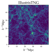
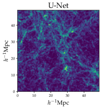
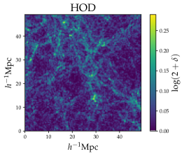
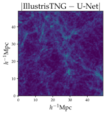
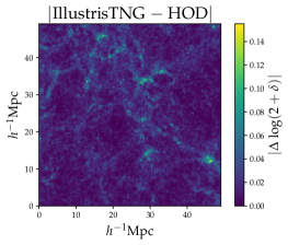
In this section we present the results our the neural network and its comparison with the HOD model.

We have reserved the sub-cubes corresponding to a larger cube of side 48 $\,h^{-1}\,{\rm Mpc}$ in the IllustrisTNG simulation volume for testing our network. Once our network is trained, we concatenate the generated Hi  field corresponding to all the sub-cubes and use the larger cube to compare the summary statistics. A possible concern could be that the stacking of the individual Hi  boxes to make a larger box can lead to spurious edge effects in the summary statistics, but we have checked that such effects are negligible, see Appendix A.4 for further details.

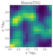
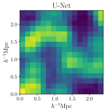
We first show a visual comparison of the network output in Figure 2. In the bottom panels we have averaged over the absolute values of the differences in the fields along the projected axis. We now discuss multiple summary statistics and find that our network outperforms HOD up to the non-linear scales $k\lesssim 1$ h/Mpc in all the statistics.

5.1 HI Power Spectrum

Figure 3: Comparison between the Hi  power spectrum [left] and the cross-correlation coefficient, defined as $r_{\mathrm{(A)}}=P_{\mathrm{A-Illustris}}/\sqrt{P_{\mathrm{A}}P_{\textup{Illustris}}}$, [right] for the IllustrisTNG simulation (orange), the HOD (green) and the neural network (black). We can see that the network outperforms the HOD for both statistics on all scales.

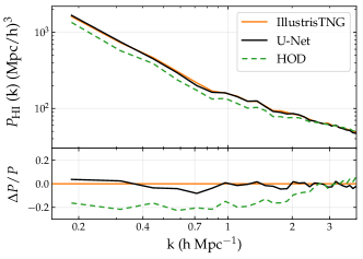
The most widely used summary statistic in cosmology is the power spectrum, which is the Fourier transform of the two-point correlation function. In 21cm IM, the quantity that is directly observed is the 21cm power spectrum, which is related to the HI power spectrum via

$$P_{\textup{21cm}}(k)=\bar{T}^{2}_{b}\,P_{\textup{HI}}(k)\,,$$ (7)

where $\bar{T}_{b}$ is the mean brightness temperature of the 21cm line at redshift $z$. Let us now compare the two terms in the RHS separately. The mean brightness temperature scales as $T_{b}\propto\Omega_{\textup{HI}}$, where $\Omega_{\textup{HI}}$ is the ratio between the density of Hi  at redshift $z$ and the Universe’s critical density at $z=0$. The network and the HOD predicts values of $10^{4}\times\Omega_{\textup{HI}}(z=1)$ in our test set to be 5.77 and 6.43, respectively, while that value is 5.82 for the IllustrisTNG simulation.

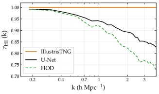
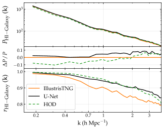
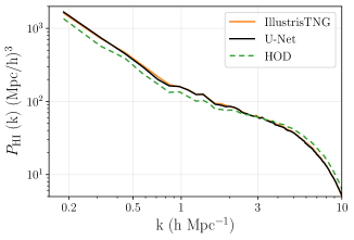
The second term to compare in Eq. (7) is $P_{\textup{HI}}(k)$, and we show the results from different methods in Figure 3. We find that the network is able to reproduce the HI power spectrum from the simulations up to a deviation of $\lesssim 5$% all the way to non-linear scales $k\lesssim 1$ $\,h\,{\rm Mpc}^{-1}$, whereas the HOD deviates by $\lesssim 20$% at low-$k$ although it becomes slightly more accurate at high-$k$. The increase in the HOD accuracy at high-$k$ arises mainly due to the 1-halo term given in Eq. (6). It is important however to note that the one-halo term in Eq. (6) only aids in the accuracy of the power spectrum (amplitude of fluctuations) at high-$k$ but not does not accurately model the phases of the Hi  fluctuations, which are relevant for the cross-correlation coefficient $r_{\textup{HI}}$ (compared in the right panel of Figure 3). VN18 argued that one possible cause of the discrepancy in the HOD power spectrum at low-$k$ may be be due to the fact that they do not explicitly fit the total $\Omega_{\textup{HI}}$ in the simulation volume, which would change the Hi  bias. However, even if the bias is changed, their $r_{\textup{HI}}$ should remain unchanged.

We do not show error bars arising from sample variance in the testing volume because the both the DM and the Hi  fields from IllustrisTNG are evolved from the same initial conditions. We chose the particular range of $k$ in Figure 3 because of the two following constraints: the low-$k$ limit is set by the largest mode in the test set (making an even larger test set is possible but at the expense of reduction in the training data), and the high-$k$ limit is conservatively set such that the scales affected by the smoothing of the Hi  maps ($\sim$ 5 $\times$ 300 $\,h^{-1}\,{\rm kpc}$) are removed (see figure 9 for $P_{\mathrm{HI}}$ plotted till $k=10\,h\,{\rm Mpc}^{-1}$).

It is worth noting that the accuracy of $P_{\rm HI}(k)$ is dependent on modeling of Hi  in high-mass halos (see for e.g. Figure 8). As mentioned in Section 3.2, the training of our network is challenging in the high-mass end, because of the sparsity associated with the the abundance of voxels in that regime. Our results can be further improved if we train the U-Net on a simulation with a larger volume, which would have a larger number of high mass halos, or using a set of zoom-in simulations focused on galaxy clusters (Thiele et al., 2020).

Let us now estimate, very crudely, the accuracy of the power spectrum model required for future 21cm surveys using some fisher forecasts in the literature. Obuljen et al. (2018) showed the peak signal-to-noise ratio (S/N) could be $\sim 10$ for upcoming surveys like HIRAX and CHIME (note that S/N will be much larger for future surveys like SKA), and therefore the accuracy of the method to produce 21cm mocks should roughly be $\lesssim 10\%$ for the power spectrum.

5.2 Cross-correlation with galaxies and halos

Large regions of future Hi  surveys will overlap with regions sampled by galaxy spectroscopic surveys like DESI or Euclid. One of the most important summary statistic in such overlapping regions is the Hi  -galaxy cross-power $P_{\textup{HI}-\textup{Galaxy}}$. Using the cross-correlations will boost the S/N ratio and mitigate the effects of foregrounds (e.g. Villaescusa-Navarro et al. (2015b) predict the S/N for the cross-correlation between future 21cm surveys and Lyman-Break galaxies to be larger than 21cm auto-correlation by a factor of $\sim 10$ ($\sim$ 4) at large (small) scales; see also Padmanabhan et al. (2020); Modi et al. (2021)). Furthermore, unlike the auto-power spectrum of 21cm which is yet to be detected, there have already been multiple detections of the $P_{\textup{HI}-\textup{Galaxy}}$ signal (Chang et al., 2010; Masui et al., 2013; Anderson et al., 2018).

In Figure 4, we compare $P_{\textup{HI}-\textup{Galaxy}}$ from our approach. We have included all the galaxies in the TNG100-1 sample with the stellar mass M${}_{*}>10^{10}$ M_⊙ (which roughly corresponds to a number density of $n=10^{-3}$ h³/Mpc³) for this measurement. Similar to the $P_{\textup{HI}}(k)$ in Figure 3, the $P_{\textup{HI}-\textup{Galaxy}}$ exhibits a bias for the HOD at low-$k$.

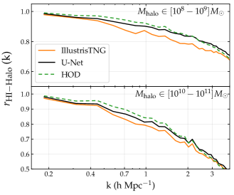
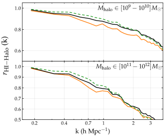
Another important statistic along the same lines is cross-correlation coefficient of Hi  with halos, which is more sensitive to the way Hi  mass is distributed across halos and to the one-halo term. We see in Figure 5 that the U-Net outperforms the HOD up to $k\lesssim$ 1 h/Mpc for all bins of halo masses that we have considered. It is worthwhile to note that if we extend Figures 4 and 5 for $k>4\,h\,{\rm Mpc}^{-1}$, the green HOD curve diverges further away from the orange IllustrisTNG curve. It is therefore likely a coincidence that the HOD outperforms the U-Net for $1\lesssim k\lesssim 4\,h\,{\rm Mpc}^{-1}$, as the green curve is merely crossing the orange curve to the other side. However, we do not show the scales $k>4\,h\,{\rm Mpc}^{-1}$ as they are affected by the smoothing of Hi  maps and a high-resolution test has to be performed to be definitive.

Figure 4: Comparison of the Hi  - galaxy cross power (upper panel), its relative error (middle), and the Hi  - galaxy cross correlation coefficient (lower), which is defined as $r_{\textup{HI - Galaxy}}=P_{\textup{HI}-\textup{Galaxy}}/\sqrt{P_{\textup{HI}}P_{\textup{Galaxy}}}$). The line labels are same as in Figure 3. The network outperforms HOD up to the non-linear scales ($k\lesssim$ 1 $\,h\,{\rm Mpc}^{-1}$).

Figure 5: Hi  - halo cross correlation coefficient ($r_{\textup{HI - Halo}}=P_{\textup{HI}-\textup{Halo}}/\sqrt{P_{\textup{HI}}P_{\textup{Halo}}}$) for multiple halo mass bins. Line labels are same as in Fig. 3. The network consistently outperforms the HOD up to non-linear scales ($k\lesssim 1\,h\,{\rm Mpc}^{-1}$).

5.3 HI Bispectrum

If all the fluctuations in the Universe were perfectly Gaussian, the field could be perfectly characterized by its two-point correlation function or its power spectrum. However, even if the primordial fluctuations were Gaussian, late-time gravitational clustering causes significant leakage of Gaussian information in the non-linear regime (Scoccimarro et al., 1999; Takada & Jain, 2004; Wadekar & Scoccimarro, 2019; Villaescusa-Navarro et al., 2019). To recover this information, the lowest order statistic that one needs to compute in Fourier space is the bispectrum. Unlike the power spectrum, the bispectrum is sensitive to the shape of the structures generated by gravitational instability and has the promise to break important degeneracies in the bias and cosmological parameters (Scoccimarro, 2000; Sefusatti et al., 2006; Hahn et al., 2020; Hahn & Villaescusa-Navarro, 2020; Yankelevich & Porciani, 2019; Chudaykin & Ivanov, 2019; Kamalinejad & Slepian, 2020). The post-reionization 21cm signal is expected to have significant information in the non-linear regime and there have been recent attempts at theoretical modeling of the Hi  bispectrum (Sarkar et al., 2019). One of the toughest parts in a bispectrum analysis is calculation of the error due to cosmic variance and a fast technique to generate mock Hi  fields is therefore essential.

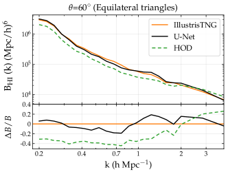
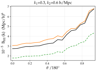
In Figure 6 we show the HI bispectrum of the IllustrisTNG simulation, together with the predictions of the HOD and neural network. We show two particular cases (which are representative of all possible triangle configurations): the first case is for equilateral triangles with different side-lengths and the second case is for triangles with a varying angle between two of its sides whose lengths are kept fixed. We checked that the results are similar for other triangle configurations. The residuals of the bispectrum of equilateral triangles from the network compared to the target is $\lesssim 20$ % for all scales we compared ($0.2<k<4\,h\,{\rm Mpc}^{-1}$), and the residuals for HOD on other hand are $\lesssim 45$ %.

Figure 6: The left panel shows the comparison of the bispectrum as a function of side length for the equilateral triangle configuration. The right panel shows the bispectrum when the angle between two particular sides of the triangle is varied keeping the length of those sides $k_{1},k_{2}$ fixed. Line labels are same as Figure 3. Note that the network is able to reproduce the bispectrum better than HOD for nearly all triangle shapes and sizes.

5.4 1-D Probability distribution function

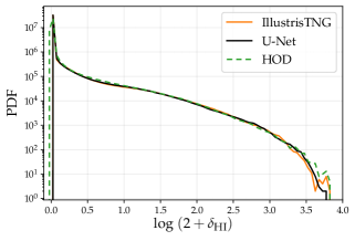
The upcoming Hi  surveys will observe systems ranging from low column densities (Ly$\alpha$ forest) to very high column densities (Damped Lyman Absorbers); the PDF of Hi  is a statistic which is sensitive to its distribution over the wide density range. The Hi  PDF can also be used for probing non-Gaussian information and for constraining luminosity functions (Breysse et al., 2017; Leicht et al., 2019). We show in Figure 7 the comparison of the U-Net prediction over four orders of magnitude of Hi  voxel masses. The comparison is difficult in the high-mass end due to sample variance: that regime is dominated by very massive halos, which are rare. Note that there is a slight discrepancy in the HOD approach for low Hi  mass voxels as it does not take into account filaments and also misses very low-mass halos which are below the simulation resolution threshold.

5.5 Abundance of HI voids

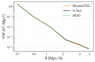
Voids are the most underdense regions of the Universe. In Figure 7 we show the void size function (VSF) of the HI field, which is defined as the number density of HI voids as a function of radius. We have used the algorithm described in Banerjee & Dalal (2016) to identify voids. The VSF is an important statistic as it contains complementary information to the one from traditional clustering observables.

Figure 7: Comparison of the 1D Hi  PDF (left) and the void size function (right). Line labels are same as Figure 3. As there are very few high mass halos in our test set volume, the high-mass tail of the PDF is dominated by sampling noise. Both our network and HOD reproduce the above statistics to a good accuracy.

6 Discussion

Let us now briefly compare our method to some other neural network approaches for emulating hydrodynamic simulations. One difference from Zamudio-Fernandez et al. (2019); Zhang et al. (2019); Yip et al. (2019); Tröster et al. (2019) is that our method can produce a hydrodynamic field of any large size (and is not restricted to the size of the input simulation box used for training the network). Zamudio-Fernandez et al. (2019) also focuses on modeling Hi  and used a generative adversarial network (GAN) to generate 3D samples of the Hi  field at redshift $z=5$ on very small scales: between 35 $\,h^{-1}\,{\rm kpc}$ and 2.34 $\,h^{-1}\,{\rm Mpc}$. However, their method cannot model the Hi  fluctuations on large scales, which are relevant for 21cm experiments. Our method, on the other hand, can model Hi  on all scales larger than $0.3$ $\,h^{-1}\,{\rm Mpc}$.

Our network takes $\sim 1.8$ hours to generate a Hi  box of side 100 $\,h^{-1}\,{\rm Mpc}$ from a given DM box on a single GPU (for comparison, the IllustrisTNG simulation takes tens of millions of CPU hours for an equivalent volume (Nelson et al., 2019)). Our method is therefore capable of making Gigaparsec volume mock Hi  fields.

It is worth mentioning some of the caveats of using deep neural networks to make mock cosmological simulations. We have trained our model to emulate a particular IllustrisTNG simulation which has fixed values of parameters for cosmology and for various baryonic feedback prescriptions. The current model also uses a high-resolution input DM field. One should be very careful with extrapolating any machine learning model beyond the range of data that it has been trained on (Pfeffer et al., 2019). It is not obvious if, without recalibration, our model can emulate a simulation with a different cosmology or baryonic feedback prescription or can work with a lower resolution input DM field. However, on the upside, our model only takes a couple of days to training to emulate a given simulation. Our technique is flexible and can quickly learn to emulate future hydrodynamic simulations which will be better than the current ones because of better technology and more observational data.

Let us discuss one interesting direction to be explored in future work. Studies have shown that the distribution of baryons inside the halos are affected by its history (for e.g. the halo formation time (Jiang & van den Bosch, 2017)). Because the U-Net is very flexible on the dimensionality of the input field, we could take into account the halo history information by including multiple DM snapshots at different redshifts as input to our U-Net. This way the U-Net would be able to approximate a function $f$ of an even more general form that the one presented in Equation (2):

$$\rho_{\rm HI}({\bf x},t)=f(\rho_{\rm m}({\bf x},t),\rho_{\rm m}({\bf x}^{\prime},t^{\prime}))$$ (8)

which implies that to predict the Hi  field at a particular point in space and time $({\bf x},t)$, the information should arise not only from the spatial vicinity ${\bf x}^{\prime}$, but also from its time evolution $t^{\prime}\leq t$.

7 Conclusions

Multiple upcoming radio telescopes such as CHIME, HIRAX, and SKA will be able to map the 21 emission from cosmic HI in the post-reionization Universe. Mock Hi  fields spanning Gigaparsec volumes are needed to provide theory predictions in the non-linear regime, to compute covariance matrices and to evaluate the effect of observational systematics like foregrounds, among many other things.

We use a deep convolutional neural network to find the mapping between the 3D fields of DM (from an N-body simulation) to Hi  (from the IllustrisTNG hydrodynamic simulation). We compared the results of our network against a state-of-the-art HOD benchmark. We show that the neural network outperforms the results of the HOD in all the summary statistics considered: power spectrum, cross-correlation coefficient, bispectrum, PDF, and void size function. While the HOD method neglects any environmental dependence on the abundance of HI inside halos, our neural network can capture any underlying pattern present. We show in our more recent paper that there is indeed a significant effect of the environment of the halo on its Hi  content, and we model it using more interpretable machine learning techniques like symbolic regression (Wadekar et al., 2020).

This study focuses on modeling Hi  in real space and we will address the modeling in redshift space in a future work. We have used a DM field from a high resolution $N$-body simulation as an input in this analysis and we plan to explore whether the U-Net technique can work on lower resolution $N$-body simulations or other approximate gravity-only simulations. Although we have focused on Hi  in this paper, we anticipate neural networks to be able to produce mocks for other line intensity mapping surveys by emulating expensive hydrodynamic simulations.

Appendix A Details and Methods

A.1 Details of network architecture

We had presented our network architecture in Figure 1 and we discuss its details in this section. Let us first discuss details of the input and the output of our network. The input DM box has a physical side length $2.34\,h^{-1}\,{\rm Mpc}$ with a grid resolution of $\sim 35\,h^{-1}\,{\rm kpc}$ and therefore has $64^{3}$ grid cells. As discussed in section 2.1, the output Hi  box has a lower resolution (physical side length of $1.17\,h^{-1}\,{\rm Mpc}$ with $8^{3}$ grid cells). A U-Net typically consists of a contracting path and an expansive path of nearly equal lengths. In our case, due to lower dimensionality of the output as compared to the input, the expansive path is relatively much shorter.

Figure 8: Comparison of histogram (left) and the power spectrum (right) on using only a single U-Net and a combination of two U-Nets (2-phase). The combination is designed to outperform a single U-Net for the high-mass Hi  voxels.

The contracting path follows the typical architecture of a convolutional neural network and consists four primary blocks. Each block consists of two successive convolutions with stride 1 and a down-sampling convolution with stride 2, each of the three is followed by batch normalization (BN) and a rectified linear unit (ReLU). For each convolutional layer, we use 3 $\times$ 3 $\times$ 3 filters. As our input DM fields are not periodic, we cannot use periodic padding similar to He et al. (2019); we instead apply a zero padding with size 1. At each down-sampling step we double the number of feature channels and reduce the number of grid-points along each dimension by a factor of 2, and vice versa for the up-sampling step.

We only have one up-sampling step in our architecture. We concatenate the up-sampled map (dimensionality $8^{3}$) with two maps from the contracting path (denoted with filled boxes): one of the same dimensionality ($8^{3}$) and an another of a higher dimensionality ($16^{3}$), but after application of a max-pooling layer. These concatenations help to train the network faster as the gradients are passed through the transverse connections. Concatenation also provides the network with various levels of granularity for the final prediction. We have also tried using a deeper neural network (which can be obtained by using stride 1 instead of stride 2 while moving between layers in figure 1), but we did not find an improvement in our results.

A.2 Two-phase model

As discussed earlier in Section 3.2, we needed to employ a two-phase model to tackle the problem of data sparsity. Let us now discuss in detail how we employ the two neural networks (labelled as FP (SP) for the first (second) phase hereafter). A simple way to think about the functions of the two networks is the following: FP fills the low Hi  mass voxels and identifies boundaries of large Hi  halos. SP is then used to assign an appropriate Hi  mass profile to the large halos.

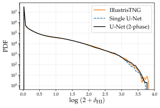
Both FP and SP have the same U-Net architecture which was shown in Figure 1. If we only use FP in our prediction, we get the results shown in a dashed line in Figure 8. From the PDF, we see that the FP is reproducing the PDF accurately for all Hi  voxels except the high-mass ones. We believe this is due to dearth of training data on the high mass Hi  voxels and expect the FP to perform better with more data. To complement FP, we choose to employ a SP which is focused on predicting only the high-mass Hi  voxels. The training of the SP is therefore a little different from that of FP. Equation (3) was used to generate rescaled fields to train the FP, but for SP, we use different rescaling transformations:

$$\begin{split}\tilde{\delta}^{(2)}_{\textup{HI}}\,&=0.03\,(1+\delta_{\textup{HI}}\,)^{0.5}\\ \tilde{\delta}^{(2)}_{\textup{DM}}&=0.0035\,(1+\delta_{\textup{DM}})^{0.25}\,.\end{split}$$ (A1)

This is because the high-mass tails of the rescaled DM and Hi  distributions are flatter for the transforms in Equation A1 as compared to Equation 3, which makes the SP easier to train in the high-mass regime. We had used the loss function in Equation 4 for training the FP. The loss function for training the SP is obtained by substituting $\tilde{\delta}\rightarrow\tilde{\delta}^{(2)}$ in Equation 4 and we find the hyper-parameters values $\beta=0.26$ and $\alpha=2.5$ give the best results for training the SP.

Let us now discuss combining the predictions of FP and SP after they are trained separately. For a given DM input field, let us denote their unscaled prediction of a particular voxel of the output Hi  field by $\delta^{\textup{FP}}$ and $\delta^{\textup{SP}}$. We get our final result for that particular voxel by combining the predictions using weights: $w^{\textup{FP}}\,\delta^{\textup{FP}}+w^{\textup{SP}}\,\delta^{\textup{SP}}$; the weights are given by

$$\begin{split}w^{\textup{FP}}&\equiv\frac{1}{1+\exp\big{[}(\delta^{\textup{SP}}-\delta^{\textup{threshold}})/100\big{]}}\\ w^{\textup{SP}}&\equiv 1-w^{\textup{FP}}\,,\end{split}$$ (A2)

and were chosen such that the output from SP is given more importance for high-mass voxels and vice versa. We have adopted $\delta^{\textup{threshold}}=1500$ for results in this paper but we checked that our results are not sensitive to the threshold in the range $\delta^{\textup{threshold}}\in$(1000 , 2000).

A.3 Training details and data augmentation

For training the network, we used the Adam optimizer (Kingma & Ba, 2014) with a learning rate ranging between $10^{-8}-10^{-4}$. The network takes nearly 30 epochs to train and we choose to use a batch-size of 28 as it was compatible with the memory constraints of our GPUs.

We also train the neural network to recognize polyhedral symmetries like translational and rotational invariance (He et al., 2019). We do this by generating multiple instances of a given input DM box by applying various symmetry transformations and then training the U-Net on all the generated cases. This process is often referred to as data augmentation because we are generating multiple training simulations given using a single data realization. We use all transformations corresponding to the symmetry group of a cube which consists of 48 elements (octahedral group of order 24 with an additional factor of 2 to account for inversion across the origin ($\vec{r}\rightarrow-\vec{r}$)). As the cubes containing high Hi  densities are rare in our training set, using data augmentation greatly helps for training in the high-density regime. We also use a popular technique for tackling data-sparsity called non-uniform sampling, where we input the cubes containing high Hi  density voxels more frequently during training. In our case, we first rank the cubes with respect to the maximum Hi  density inside them, and then increase the frequency of occurrence of the top 1% cubes by 100 fold. However, even after using data augmentation and non-uniform sampling, we still had to use the two-phase neural network approach as the data sparsity problem in our case is quite extreme.

We trained all of our models using New York University’s High Performance Cluster using NVIDIA Tesla P-100 and P-40 GPUs.

A.4 Testing edge-effects while combining HI boxes

In section 5 we showed results from the test set Hi  cube. To construct this box, we used the U-Net to generate small $1.17\,h^{-1}\,{\rm Mpc}$ side Hi  sub-cubes and then stacked them together to produce the test $48\,h^{-1}\,{\rm Mpc}$ cube. One possible concern might be that such stacking produces edge effects which will affect summary statistics at scales comparable to the length of the box ($k\sim 5\,h\,{\rm Mpc}^{-1}$). We therefore check that there indeed are no artifacts on these scales and show the high-$k$ Hi  power spectrum comparison in figure 9. Furthermore, we also show a zoom in version of the output of test cube in figure 10. A reason for the absence of edge artifacts could be the larger size of DM box used to predict a smaller Hi  box (c.f. figure 1), so information beyond the location of edges of the Hi  box is included in the U-Net prediction. We also tried using the technique of annealing when concatenating the small Hi  subcubes to smoothen their edges, but our results did not change.

Figure 9: Same as the left panel of figure 3 but extended to high-$k$ regions.

Figure 10: Same as the upper panels of figure 2 but zooming in on the lower left region of the box in order to verify that there are no spurious edge effects when Hi  subcubes of side 1.17$\,h\,{\rm Mpc}^{-1}$ are concatenated to produce the large U-Net output cube.

References

- Anderson et al. (2018) Anderson, C. J., Luciw, N. J., Li, Y. C., et al. 2018, MNRAS, 476, 3382, doi: 10.1093/mnras/sty346
- Banerjee & Dalal (2016) Banerjee, A., & Dalal, N. 2016, J. Cosmology Astropart. Phys, 2016, 015, doi: 10.1088/1475-7516/2016/11/015
- Bauer et al. (2020) Bauer, J. B., Marsh, D. J. E., Hložek, R., Padmanabhan, H., & Laguë, A. 2020, arXiv e-prints, arXiv:2003.09655. https://arxiv.org/abs/2003.09655
- Benson (2012) Benson, A. J. 2012, New A, 17, 175, doi: 10.1016/j.newast.2011.07.004
- Berlind & Weinberg (2002) Berlind, A. A., & Weinberg, D. H. 2002, ApJ, 575, 587, doi: 10.1086/341469
- Bharadwaj et al. (2001) Bharadwaj, S., Nath, B. B., & Sethi, S. K. 2001, Journal of Astrophysics and Astronomy, 22, 21, doi: 10.1007/BF02933588
- Bharadwaj & Sethi (2001) Bharadwaj, S., & Sethi, S. K. 2001, Journal of Astrophysics and Astronomy, 22, 293, doi: 10.1007/BF02702273
- Breysse et al. (2017) Breysse, P. C., Kovetz, E. D., Behroozi, P. S., Dai, L., & Kamionkowski, M. 2017, MNRAS, 467, 2996, doi: 10.1093/mnras/stx203
- Bull et al. (2015) Bull, P., Ferreira, P. G., Patel, P., & Santos, M. G. 2015, ApJ, 803, 21, doi: 10.1088/0004-637X/803/1/21
- Carleo et al. (2019) Carleo, G., Cirac, I., Cranmer, K., et al. 2019, Reviews of Modern Physics, 91, 045002, doi: 10.1103/RevModPhys.91.045002
- Carucci et al. (2017) Carucci, I. P., Corasaniti, P.-S., & Viel, M. 2017, J. Cosmology Astropart. Phys, 2017, 018, doi: 10.1088/1475-7516/2017/12/018
- Carucci et al. (2015) Carucci, I. P., Villaescusa-Navarro, F., Viel, M., & Lapi, A. 2015, J. Cosmology Astropart. Phys, 2015, 047, doi: 10.1088/1475-7516/2015/07/047
- Castorina & Villaescusa-Navarro (2017) Castorina, E., & Villaescusa-Navarro, F. 2017, MNRAS, 471, 1788, doi: 10.1093/mnras/stx1599
- Chang et al. (2010) Chang, T.-C., Pen, U.-L., Bandura, K., & Peterson, J. B. 2010, arXiv e-prints, arXiv:1007.3709. https://arxiv.org/abs/1007.3709
- Chang et al. (2008) Chang, T.-C., Pen, U.-L., Peterson, J. B., & McDonald, P. 2008, Phys. Rev. Lett., 100, 091303, doi: 10.1103/PhysRevLett.100.091303
- Chardin et al. (2019) Chardin, J., Uhlrich, G., Aubert, D., et al. 2019, MNRAS, 490, 1055, doi: 10.1093/mnras/stz2605
- Chudaykin & Ivanov (2019) Chudaykin, A., & Ivanov, M. M. 2019, J. Cosmology Astropart. Phys, 2019, 034, doi: 10.1088/1475-7516/2019/11/034
- Dalal et al. (2008) Dalal, N., Doré, O., Huterer, D., & Shirokov, A. 2008, Phys. Rev. D, 77, 123514, doi: 10.1103/PhysRevD.77.123514
- Gao et al. (2005) Gao, L., Springel, V., & White, S. D. M. 2005, MNRAS, 363, L66, doi: 10.1111/j.1745-3933.2005.00084.x
- Gillet et al. (2019) Gillet, N., Mesinger, A., Greig, B., Liu, A., & Ucci, G. 2019, MNRAS, 484, 282, doi: 10.1093/mnras/stz010
- Giusarma et al. (2019) Giusarma, E., Reyes Hurtado, M., Villaescusa-Navarro, F., et al. 2019, arXiv e-prints, arXiv:1910.04255. https://arxiv.org/abs/1910.04255
- Hadzhiyska et al. (2020) Hadzhiyska, B., Bose, S., Eisenstein, D., Hernquist, L., & Spergel, D. N. 2020, MNRAS, 493, 5506, doi: 10.1093/mnras/staa623
- Hahn & Villaescusa-Navarro (2020) Hahn, C., & Villaescusa-Navarro, F. 2020, arXiv e-prints, arXiv:2012.02200. https://arxiv.org/abs/2012.02200
- Hahn et al. (2020) Hahn, C., Villaescusa-Navarro, F., Castorina, E., & Scoccimarro, R. 2020, J. Cosmology Astropart. Phys, 2020, 040, doi: 10.1088/1475-7516/2020/03/040
- Hassan et al. (2020) Hassan, S., Andrianomena, S., & Doughty, C. 2020, MNRAS, 494, 5761, doi: 10.1093/mnras/staa1151
- He et al. (2019) He, S., Li, Y., Feng, Y., et al. 2019, Proceedings of the National Academy of Science, 116, 13825, doi: 10.1073/pnas.1821458116
- Hornik et al. (1989) Hornik, K., Stinchcombe, M., & White, H. 1989, Neural Networks, 2, 359, doi: https://doi.org/10.1016/0893-6080(89)90020-8
- Jiang & van den Bosch (2017) Jiang, F., & van den Bosch, F. C. 2017, MNRAS, 472, 657, doi: 10.1093/mnras/stx1979
- Kamalinejad & Slepian (2020) Kamalinejad, F., & Slepian, Z. 2020, arXiv e-prints, arXiv:2011.00899. https://arxiv.org/abs/2011.00899
- Karagiannis et al. (2019) Karagiannis, D., Slosar, A., & Liguori, M. 2019, arXiv e-prints, arXiv:1911.03964. https://arxiv.org/abs/1911.03964
- Kingma & Ba (2014) Kingma, D. P., & Ba, J. 2014, arXiv e-prints, arXiv:1412.6980. https://arxiv.org/abs/1412.6980
- Kodi Ramanah et al. (2020) Kodi Ramanah, D., Charnock, T., Villaescusa-Navarro, F., & Wandelt, B. D. 2020, MNRAS, 495, 4227, doi: 10.1093/mnras/staa1428
- Kwon et al. (2020) Kwon, Y., Hong, S. E., & Park, I. 2020, arXiv e-prints, arXiv:2006.06236. https://arxiv.org/abs/2006.06236
- Leicht et al. (2019) Leicht, O., Uhlemann, C., Villaescusa-Navarro, F., et al. 2019, MNRAS, 484, 269, doi: 10.1093/mnras/sty3469
- List & Lewis (2020) List, F., & Lewis, G. F. 2020, MNRAS, 493, 5913, doi: 10.1093/mnras/staa523
- Mangena et al. (2020) Mangena, T., Hassan, S., & Santos, M. G. 2020, MNRAS, 494, 600, doi: 10.1093/mnras/staa750
- Masui et al. (2013) Masui, K. W., Switzer, E. R., Banavar, N., et al. 2013, ApJ, 763, L20, doi: 10.1088/2041-8205/763/1/L20
- Modi et al. (2019a) Modi, C., Castorina, E., Feng, Y., & White, M. 2019a, J. Cosmology Astropart. Phys, 2019, 024, doi: 10.1088/1475-7516/2019/09/024
- Modi et al. (2020) Modi, C., Chen, S.-F., & White, M. 2020, MNRAS, 492, 5754, doi: 10.1093/mnras/staa251
- Modi et al. (2018) Modi, C., Feng, Y., & Seljak, U. 2018, J. Cosmology Astropart. Phys, 2018, 028, doi: 10.1088/1475-7516/2018/10/028
- Modi et al. (2021) Modi, C., White, M., Castorina, E., & Slosar, A. 2021, arXiv e-prints, arXiv:2102.08116. https://arxiv.org/abs/2102.08116
- Modi et al. (2019b) Modi, C., White, M., Slosar, A., & Castorina, E. 2019b, J. Cosmology Astropart. Phys, 2019, 023, doi: 10.1088/1475-7516/2019/11/023
- Nelson et al. (2019) Nelson, D., Pillepich, A., Springel, V., et al. 2019, Mon. Not. Roy. Astron. Soc., 490, 3234, doi: 10.1093/mnras/stz2306
- Ntampaka et al. (2019) Ntampaka, M., et al. 2019. https://arxiv.org/abs/1902.10159
- Obuljen et al. (2018) Obuljen, A., Castorina, E., Villaescusa-Navarro, F., & Viel, M. 2018, J. Cosmology Astropart. Phys, 2018, 004, doi: 10.1088/1475-7516/2018/05/004
- Padmanabhan et al. (2016) Padmanabhan, H., Choudhury, T. R., & Refregier, A. 2016, MNRAS, 458, 781, doi: 10.1093/mnras/stw353
- Padmanabhan et al. (2020) Padmanabhan, H., Refregier, A., & Amara, A. 2020, MNRAS, 495, 3935, doi: 10.1093/mnras/staa1373
- Paranjape et al. (2018) Paranjape, A., Hahn, O., & Sheth, R. K. 2018, MNRAS, 476, 3631, doi: 10.1093/mnras/sty496
- Peacock & Smith (2000) Peacock, J. A., & Smith, R. E. 2000, MNRAS, 318, 1144, doi: 10.1046/j.1365-8711.2000.03779.x
- Peterson et al. (2009) Peterson, J. B., et al. 2009, 21 cm Intensity Mapping. https://arxiv.org/abs/0902.3091
- Pfeffer et al. (2019) Pfeffer, D. N., Breysse, P. C., & Stein, G. 2019, arXiv e-prints, arXiv:1905.10376. https://arxiv.org/abs/1905.10376
- Pillepich et al. (2018) Pillepich, A., Springel, V., Nelson, D., et al. 2018, MNRAS, 473, 4077, doi: 10.1093/mnras/stx2656
- Pullen et al. (2014) Pullen, A. R., Doré, O., & Bock, J. 2014, ApJ, 786, 111, doi: 10.1088/0004-637X/786/2/111
- Ravanbakhsh et al. (2017) Ravanbakhsh, S., Oliva, J., Fromenteau, S., et al. 2017, arXiv e-prints, arXiv:1711.02033. https://arxiv.org/abs/1711.02033
- Ronneberger et al. (2015) Ronneberger, O., Fischer, P., & Brox, T. 2015, arXiv e-prints, arXiv:1505.04597. https://arxiv.org/abs/1505.04597
- Sarkar et al. (2019) Sarkar, D., Majumdar, S., & Bharadwaj, S. 2019, MNRAS, 490, 2880, doi: 10.1093/mnras/stz2799
- Schmittfull et al. (2019) Schmittfull, M., Simonović, M., Assassi, V., & Zaldarriaga, M. 2019, Phys. Rev. D, 100, 043514, doi: 10.1103/PhysRevD.100.043514
- Scoccimarro (2000) Scoccimarro, R. 2000, ApJ, 544, 597, doi: 10.1086/317248
- Scoccimarro et al. (2001) Scoccimarro, R., Sheth, R. K., Hui, L., & Jain, B. 2001, ApJ, 546, 20, doi: 10.1086/318261
- Scoccimarro et al. (1999) Scoccimarro, R., Zaldarriaga, M., & Hui, L. 1999, ApJ, 527, 1, doi: 10.1086/308059
- Sefusatti et al. (2006) Sefusatti, E., Crocce, M., Pueblas, S., & Scoccimarro, R. 2006, Phys. Rev. D, 74, 023522, doi: 10.1103/PhysRevD.74.023522
- Seljak (2000) Seljak, U. 2000, MNRAS, 318, 203, doi: 10.1046/j.1365-8711.2000.03715.x
- Sheth & Tormen (2004) Sheth, R. K., & Tormen, G. 2004, MNRAS, 350, 1385, doi: 10.1111/j.1365-2966.2004.07733.x
- Shimabukuro & Semelin (2017) Shimabukuro, H., & Semelin, B. 2017, MNRAS, 468, 3869, doi: 10.1093/mnras/stx734
- Sinigaglia et al. (2020) Sinigaglia, F., Kitaura, F.-S., Balaguera-Antolínez, A., et al. 2020, arXiv e-prints, arXiv:2012.06795. https://arxiv.org/abs/2012.06795
- Spinelli et al. (2020) Spinelli, M., Zoldan, A., De Lucia, G., Xie, L., & Viel, M. 2020, MNRAS, 493, 5434, doi: 10.1093/mnras/staa604
- Takada & Jain (2004) Takada, M., & Jain, B. 2004, MNRAS, 348, 897, doi: 10.1111/j.1365-2966.2004.07410.x
- Thiele et al. (2020) Thiele, L., Villaescusa-Navarro, F., Spergel, D. N., Nelson, D., & Pillepich, A. 2020, arXiv e-prints, arXiv:2007.07267. https://arxiv.org/abs/2007.07267
- Tröster et al. (2019) Tröster, T., Ferguson, C., Harnois-Déraps, J., & McCarthy, I. G. 2019, MNRAS, 487, L24, doi: 10.1093/mnrasl/slz075
- Villaescusa-Navarro et al. (2017) Villaescusa-Navarro, F., Alonso, D., & Viel, M. 2017, MNRAS, 466, 2736, doi: 10.1093/mnras/stw3224
- Villaescusa-Navarro et al. (2015a) Villaescusa-Navarro, F., Bull, P., & Viel, M. 2015a, ApJ, 814, 146, doi: 10.1088/0004-637X/814/2/146
- Villaescusa-Navarro et al. (2015b) Villaescusa-Navarro, F., Viel, M., Alonso, D., et al. 2015b, J. Cosmology Astropart. Phys, 2015, 034, doi: 10.1088/1475-7516/2015/03/034
- Villaescusa-Navarro et al. (2014) Villaescusa-Navarro, F., Viel, M., Datta, K. K., & Choudhury, T. R. 2014, J. Cosmology Astropart. Phys, 2014, 050, doi: 10.1088/1475-7516/2014/09/050
- Villaescusa-Navarro et al. (2018) Villaescusa-Navarro, F., Genel, S., Castorina, E., et al. 2018, ApJ, 866, 135, doi: 10.3847/1538-4357/aadba0
- Villaescusa-Navarro et al. (2019) Villaescusa-Navarro, F., Hahn, C., Massara, E., et al. 2019, arXiv e-prints, arXiv:1909.05273. https://arxiv.org/abs/1909.05273
- Villanueva-Domingo & Villaescusa-Navarro (2020) Villanueva-Domingo, P., & Villaescusa-Navarro, F. 2020, arXiv e-prints, arXiv:2006.14305. https://arxiv.org/abs/2006.14305
- Wadekar & Scoccimarro (2019) Wadekar, D., & Scoccimarro, R. 2019, arXiv e-prints, arXiv:1910.02914. https://arxiv.org/abs/1910.02914
- Wadekar et al. (2020) Wadekar, D., Villaescusa-Navarro, F., Ho, S., & Perreault-Levasseur, L. 2020, arXiv e-prints, arXiv:2012.00111. https://arxiv.org/abs/2012.00111
- Wechsler et al. (2006) Wechsler, R. H., Zentner, A. R., Bullock, J. S., Kravtsov, A. V., & Allgood, B. 2006, ApJ, 652, 71, doi: 10.1086/507120
- Weinberger et al. (2017) Weinberger, R., Springel, V., Hernquist, L., et al. 2017, MNRAS, 465, 3291, doi: 10.1093/mnras/stw2944
- Yankelevich & Porciani (2019) Yankelevich, V., & Porciani, C. 2019, MNRAS, 483, 2078, doi: 10.1093/mnras/sty3143
- Yip et al. (2019) Yip, J. H. T., Zhang, X., Wang, Y., et al. 2019, arXiv e-prints, arXiv:1910.07813. https://arxiv.org/abs/1910.07813
- Zamudio-Fernandez et al. (2019) Zamudio-Fernandez, J., Okan, A., Villaescusa-Navarro, F., et al. 2019, arXiv e-prints, arXiv:1904.12846. https://arxiv.org/abs/1904.12846
- Zhang et al. (2019) Zhang, X., Wang, Y., Zhang, W., et al. 2019, arXiv e-prints, arXiv:1902.05965. https://arxiv.org/abs/1902.05965