Bootstrap Bounds on Closed Einstein Manifolds

James Bonifacio,***james.bonifacio@case.edu and Kurt Hinterbichler,kurt.hinterbichler@case.edu

CERCA, Department of Physics,

Case Western Reserve University, 10900 Euclid Ave, Cleveland, OH 44106

Abstract

A compact Riemannian manifold is associated with geometric data given by the eigenvalues of various Laplacian operators on the manifold and the triple overlap integrals of the corresponding eigenmodes. This geometric data must satisfy certain consistency conditions that follow from associativity and the completeness of eigenmodes. We show that it is possible to obtain nontrivial bounds on the geometric data of closed Einstein manifolds by using semidefinite programming to study these consistency conditions, in analogy to the conformal bootstrap bounds on conformal field theories. These bootstrap bounds translate to constraints on the tree-level masses and cubic couplings of Kaluza–Klein modes in theories with compact extra dimensions. We show that in some cases the bounds are saturated by known manifolds.

1 Introduction

There are several cases of historically intractable problems in physics which have seen significant recent progress arise from a numerical bootstrap approach. To employ such an approach, one starts with some general principles, derives from them consistency conditions that the observable quantities of interest must satisfy, and then solves these consistency conditions numerically on a computer. This gives general constraints on the possible values that the observables can take. Examples of interesting physical systems that have been recently studied using such methods include strongly coupled conformal field theories (CFTs) [1], scattering amplitudes [2, 3], and random matrix models [4]. These studies have given information about these systems which is generally out of reach of traditional perturbative methods.

In this paper we show that it is possible to apply a similar numerical bootstrap approach to obtain nontrivial mathematical results about closed Einstein manifolds. A closed Einstein manifold \mathcal{M} is a compact smooth manifold without boundary that is equipped with a metric gmnsubscript𝑔𝑚𝑛g_{mn} whose Ricci curvature satisfies Rmn=λgmnsubscript𝑅𝑚𝑛𝜆subscript𝑔𝑚𝑛R_{mn}=\lambda g_{mn} for some constant λ𝜆\lambda. We limit our consideration to closed Einstein manifolds that are connected and orientable, as well as the quotients of such manifolds by isometry subgroups. We find new bounds on the geometric data associated with such manifolds. Specifically, the bounds involve the spectrum of eigenvalues of various Laplacian operators and the triple overlap integrals of their eigenmodes.

Our bounds come from studying certain consistency conditions involving the geometric data. For a simple example of these consistency conditions, consider the scalar Laplacian, ΔΔ\Delta. A scalar eigenfunction ψasubscript𝜓𝑎\psi_{a} with eigenvalue λasubscript𝜆𝑎\lambda_{a} satisfies the eigenvalue equation Δψa=λaψaΔsubscript𝜓𝑎subscript𝜆𝑎subscript𝜓𝑎\Delta\psi_{a}=\lambda_{a}\psi_{a}. For any three eigenfunctions we can construct the following triple overlap integral:

ga1a2a3ψa1ψa2ψa3.subscript𝑔subscript𝑎1subscript𝑎2subscript𝑎3subscriptsubscript𝜓subscript𝑎1subscript𝜓subscript𝑎2subscript𝜓subscript𝑎3g_{a_{1}a_{2}a_{3}}\equiv\int_{\mathcal{M}}\psi_{a_{1}}\psi_{a_{2}}\psi_{a_{3}}. (1.1)

The eigenfunctions can be chosen so that they form an orthonormal basis, so we can write the product ψa1ψa2subscript𝜓subscript𝑎1subscript𝜓subscript𝑎2\psi_{a_{1}}\psi_{a_{2}} as a sum over eigenmodes

ψa1ψa2=aga1a2ψaa,subscript𝜓subscript𝑎1subscript𝜓subscript𝑎2subscript𝑎subscript𝑔subscript𝑎1subscript𝑎2superscriptsubscript𝜓𝑎𝑎\psi_{a_{1}}\psi_{a_{2}}=\sum_{a}g_{a_{1}a_{2}}{}^{a}\psi_{a}\,, (1.2)

where orthonormality gives the coefficients as the triple overlap integrals (1.1). By repeatedly applying (1.2) to pairs of eigenmodes, integrals involving products of four or more eigenfunctions can be reduced to sums of products of the triple overlap integrals. For example, we can write

ψa1ψa2ψa3ψa4=aga1a2ga3a4aa,subscriptsubscript𝜓subscript𝑎1subscript𝜓subscript𝑎2subscript𝜓subscript𝑎3subscript𝜓subscript𝑎4subscript𝑎subscript𝑔subscript𝑎1subscript𝑎2superscriptsubscript𝑔subscript𝑎3subscript𝑎4𝑎𝑎\int_{\mathcal{M}}\psi_{a_{1}}\psi_{a_{2}}\psi_{a_{3}}\psi_{a_{4}}=\sum_{a}g_{a_{1}a_{2}}{}{}^{a}g_{a_{3}a_{4}a}\,, (1.3)

where we used the completeness relation (1.2) on ψa1ψa2subscript𝜓subscript𝑎1subscript𝜓subscript𝑎2\psi_{a_{1}}\psi_{a_{2}} and ψa3ψa4subscript𝜓subscript𝑎3subscript𝜓subscript𝑎4\psi_{a_{3}}\psi_{a_{4}}. Now the key point is that this expansion can be done in other ways by pairing different eigenfunctions. Equating the resulting expressions then gives consistency conditions for the triple overlap integrals. For example, exchanging a2a3subscript𝑎2subscript𝑎3a_{2}\leftrightarrow a_{3} in Eq. (1.3) and equating with the original result gives

aga1a2ga3a4aa=aga1a3ga2a4aa.subscript𝑎subscript𝑔subscript𝑎1subscript𝑎2superscriptsubscript𝑔subscript𝑎3subscript𝑎4𝑎𝑎subscript𝑎subscript𝑔subscript𝑎1subscript𝑎3superscriptsubscript𝑔subscript𝑎2subscript𝑎4𝑎𝑎\sum_{a}g_{a_{1}a_{2}}{}{}^{a}g_{a_{3}a_{4}a}=\sum_{a}g_{a_{1}a_{3}}{}{}^{a}g_{a_{2}a_{4}a}\,. (1.4)

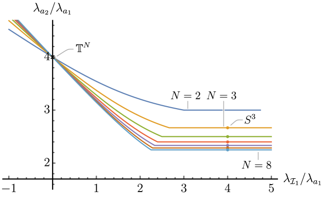
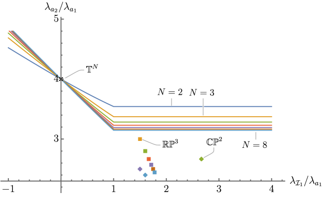
Consistency conditions of the form (1.4) will be the basic relations that we exploit to get bootstrap bounds on the geometric data. By considering quartic overlap integrals involving derivatives of scalar eigenfunctions, we will find consistency conditions that are much more complicated and involve various triple overlap integrals and eigenvalues. The consistency conditions usually cannot be solved directly, but we can extract nontrivial bounds by reformulating them as a semidefinite program. An example of such a bound is shown in Figure 1, which shows numerical upper bounds on the ratio of the first two distinct non-vanishing eigenvalues of the scalar Laplacian on closed Einstein manifolds with non-negative scalar curvature as a function of the smallest Lichnerowicz eigenvalue on transverse traceless tensors. We obtain many different bounds of this sort on eigenvalues and triple overlap integrals, both numerical and exact.

There is a sharp analogy between this geometry bootstrap and the modern conformal bootstrap [1] (see Ref. [5] for a recent review), which heavily inspires our approach. The geometric data we consider is analogous to the conformal data that defines a CFT: the eigenmodes are analogous to CFT operators, their eigenvalues are analogous to the conformal dimensions, and their triple overlap integrals are analogous to the operator product expansion (OPE) coefficients. The eigenfunction expansions such as (1.2) are like the OPE in a CFT and the consistency conditions such as (1.4) are like the crossing relations that form the basis of the modern CFT bootstrap. See Table 1 for a summary of this analogy.

Einstein manifolds CFTs
 Laplacian eigenmodes Primary operators
Eigenvalues Scaling dimensions
Triple overlap integrals OPE coefficients
Eigenfunction expansion OPE
Consistency conditions Crossing equations
Lichnerowicz bound Unitarity bound
Table 1: An analogy between Einstein manifolds and CFTs.

There are many existing results concerning the spectrum of eigenvalues of Laplacian operators on compact Riemannian manifolds [6], but bounds on the triple overlap integrals are less well studied. As far as we know, the bounds we find for Einstein manifolds are not known in the mathematical literature. Often it is difficult to determine explicitly the eigenvalues and eigenfunctions of a given manifold (see Appendix A for some exceptions). For example, for compact Calabi–Yau manifolds there are no nontrivial examples for which the spectrum of the scalar Laplacian is known analytically and numerical methods must be used [7]. One numerical method for computing the low-lying eigenvalues is to use Donaldson’s algorithm to approximate the Ricci-flat Kähler metric [8, 9], as in Ref. [10]. This is what one might call a Monte Carlo approach, where accurate results are obtained for a specific manifold. In contrast, the bootstrap approach is able to find bounds that apply to all Einstein manifolds satisfying a few assumptions.

While the results we derive can be considered as purely mathematical results about closed Einstein manifolds, there is also a physical interpretation in terms of Kaluza–Klein theories. Starting with a higher-dimensional theory on a product spacetime, one can integrate over any compact extra dimensions to obtain an equivalent lower-dimensional theory. This lower-dimensional theory will contain towers of particles of various spins which correspond to the excitations of the higher-dimensional fields in the extra dimensions. The masses of these Kaluza–Klein modes are determined by the eigenvalues of Laplacians on the internal manifold and the strengths of their three-point interactions are determined by the triple overlap integrals of the eigenmodes. In the case where the internal manifold is Einstein, the mathematical bounds on eigenvalues and overlap integrals we obtain thus translate into bounds on the tree-level masses and cubic interactions of these Kaluza–Klein modes. This is the case, for example, in reductions of pure gravity and for Calabi–Yau reductions of supergravity.

Conventions: We use the Einstein summation convention for spatial indices n,m,𝑛𝑚n,m,\dots but not for the indices a𝑎a, i𝑖i, \mathcal{I} labelling eigenfunctions. We (anti)symmetrize with weight one. The curvature conventions are those of Ref. [11].

2 Geometry review

We start by setting our notation and reviewing some basic Riemannian geometry that we need for the rest of the paper. We also review the geometric consistency conditions discussed in Ref. [12].

2.1 Einstein manifolds

Let \mathcal{M} be an N𝑁N-dimensional Einstein manifold, with metric gmnsubscript𝑔𝑚𝑛g_{mn}, that is connected, orientable, and closed (compact without boundary). We denote the volume of \mathcal{M} by V𝑉V and its Ricci curvature by Rmnsubscript𝑅𝑚𝑛R_{mn}. By definition, an Einstein manifold satisfies

Rmn=λgmn,subscript𝑅𝑚𝑛𝜆subscript𝑔𝑚𝑛R_{mn}=\lambda g_{mn}\,, (2.1)

where λ𝜆\lambda is a real constant. Taking the trace of Eq. (2.1) shows that the Ricci scalar R𝑅R is also constant, given by R=Nλ𝑅𝑁𝜆R=N\lambda. Einstein manifolds with R=0𝑅0R=0 are called Ricci-flat manifolds.

Einstein manifolds are solutions to the vacuum Einstein equations with a possibly nonzero cosmological constant. For this work we are interested in the case of Riemannian Einstein manifolds and their application as the compact spatial dimensions of a Lorentzian Kaluza–Klein product spacetime. The case N=1𝑁1N=1 would require a separate treatment for many of our formulae and is already completely understood (it is just the circle), so henceforth we restrict to N2𝑁2N\geq 2. See Ref. [13] for a classic reference on Einstein manifolds.

2.2 Laplacians

We need to introduce three different Laplacian operators on the closed Einstein manifold \mathcal{M}: the scalar Laplacian, the vector Hodge Laplacian, and the Lichnerowicz Laplacian on tensors. These are self-adjoint elliptic operators (with respect to the appropriate inner products), so we can use standard results of spectral theory on compact manifolds. For example, on any given manifold each Laplacian has a discrete spectrum that is bounded from below and unbounded from above and there exists a basis of real orthonormal eigenmodes. In Kaluza–Klein theories these eigenmodes correspond to different particles and their eigenvalues determine the masses of the particles (see, e.g., Ref. [14] for details).

Scalar Laplacian

We denote by ψasubscript𝜓𝑎\psi_{a} an orthonormal basis of non-constant real eigenfunctions of the scalar Laplacian on \mathcal{M}, where a𝑎a is a discrete index labelling the different eigenfunctions. These eigenfunctions satisfy

Δψaψa=λaψa,Δsubscript𝜓𝑎subscript𝜓𝑎subscript𝜆𝑎subscript𝜓𝑎\Delta\psi_{a}\equiv-\Box\psi_{a}=\lambda_{a}\psi_{a}, (2.2)

where λa>0subscript𝜆𝑎0\lambda_{a}>0 is the corresponding eigenvalue. Orthonormality implies that

ψa1ψa2=δa1a2,subscriptsubscript𝜓subscript𝑎1subscript𝜓subscript𝑎2subscript𝛿subscript𝑎1subscript𝑎2\int_{\mathcal{M}}\psi_{a_{1}}\psi_{a_{2}}=\delta_{a_{1}a_{2}}, (2.3)

where subscript\int_{\mathcal{M}} denotes the integral over \mathcal{M} with the canonical volume form. The normalized constant eigenfunction is V1/2superscript𝑉12V^{-1/2}. This is the unique zero mode for the scalar Laplacian and we now treat it separately from the non-constant eigenfunctions (unlike in the introduction). Completeness tells us that any L2superscript𝐿2L^{2}-normalizable scalar function ϕitalic-ϕ\phi on {\cal M} can be expanded as

ϕ=c0V1/2+acaψa,italic-ϕsuperscript𝑐0superscript𝑉12subscript𝑎superscript𝑐𝑎subscript𝜓𝑎\phi=\frac{c^{0}}{V^{1/2}}+\sum_{a}c^{a}\psi_{a}, (2.4)

where c0=V1/2ϕsuperscript𝑐0superscript𝑉12subscriptitalic-ϕc^{0}=V^{-1/2}\int_{\mathcal{M}}\phi and ca=ϕψasuperscript𝑐𝑎subscriptitalic-ϕsuperscript𝜓𝑎c^{a}=\int_{\mathcal{M}}\phi\psi^{a}.

There are special eigenfunctions of the scalar Laplacian called conformal scalars, which are defined as those scalars whose gradients are conformal Killing vectors that are not Killing vectors. We index these by the set Iconf.subscript𝐼confI_{\rm conf.}. Conformal scalars satisfy the equation

(mn1Ngmn)ψa=0,aIconf.,formulae-sequencesubscript𝑚subscript𝑛1𝑁subscript𝑔𝑚𝑛subscript𝜓𝑎0𝑎subscript𝐼conf\left(\nabla_{m}\nabla_{n}-\frac{1}{N}g_{mn}\Box\right)\psi_{a}=0,\quad a\in I_{\rm conf.}, (2.5)

and they exist only on the round spheres [15]. The conformal scalars are precisely the L=1𝐿1L=1 spherical harmonics on SNsuperscript𝑆𝑁S^{N} if N>1𝑁1N>1 (see Appendix A).111There can be many inequivalent Einstein metrics on spheres and exotic spheres [16]. By SNsuperscript𝑆𝑁S^{N} we will mean the sphere with the standard round metric unless stated otherwise.

On Einstein manifolds with R>0𝑅0R>0 the Lichnerowicz bound gives [17]

λaRN1,subscript𝜆𝑎𝑅𝑁1\lambda_{a}\geq\frac{R}{N-1}, (2.6)

and this is saturated only by conformal scalars. This is analogous to a CFT unitarity bound.

Vector Laplacian

Denote by Ym,isubscript𝑌𝑚𝑖Y_{m,i} an orthonormal basis of real, transverse eigenvectors of the one-form Hodge Laplacian on \mathcal{M}, where i𝑖i is a discrete index labelling the different eigenvectors. These eigenvectors satisfy

ΔYm,iYm,i+RmYn,in=λiYm,i,mYm,i=0,formulae-sequenceΔsubscript𝑌𝑚𝑖subscript𝑌𝑚𝑖subscript𝑅𝑚superscriptsubscript𝑌𝑛𝑖𝑛subscript𝜆𝑖subscript𝑌𝑚𝑖superscript𝑚subscript𝑌𝑚𝑖0\Delta Y_{m,i}\equiv-\Box Y_{m,i}+R_{m}{}^{n}Y_{n,i}=\lambda_{i}Y_{m,i},\quad\nabla^{m}Y_{m,i}=0, (2.7)

where λi0subscript𝜆𝑖0\lambda_{i}\geq 0 is the corresponding eigenvalue. Orthonormality implies that

Ym,i1Yi2m=δi1i2.subscriptsubscript𝑌𝑚subscript𝑖1subscriptsuperscript𝑌𝑚subscript𝑖2subscript𝛿subscript𝑖1subscript𝑖2\int_{\mathcal{M}}Y_{m,i_{1}}Y^{m}_{i_{2}}=\delta_{i_{1}i_{2}}. (2.8)

Using completeness and the Hodge decomposition, any one-form Vmsubscript𝑉𝑚V_{m} on {\cal M} can be expanded as

Vm=iciYm,i+acamψa,subscript𝑉𝑚subscript𝑖superscript𝑐𝑖subscript𝑌𝑚𝑖subscript𝑎superscript𝑐𝑎subscript𝑚subscript𝜓𝑎V_{m}=\sum_{i}c^{i}Y_{m,i}+\sum_{a}c^{a}\partial_{m}\psi_{a}, (2.9)

where ci=VmYimsuperscript𝑐𝑖subscriptsubscript𝑉𝑚subscriptsuperscript𝑌𝑚𝑖c^{i}=\int_{\mathcal{M}}V_{m}Y^{m}_{i} and ca=λa1Vmmψasuperscript𝑐𝑎superscriptsubscript𝜆𝑎1subscriptsubscript𝑉𝑚superscript𝑚subscript𝜓𝑎c^{a}=\lambda_{a}^{-1}\int_{\mathcal{M}}V_{m}\partial^{m}\psi_{a}.

Killing vectors are special transverse eigenvectors that generate the isometries of the metric. We index them by the set IKillingsubscript𝐼KillingI_{\rm Killing}. They satisfy the Killing equation,

(mYn),i=0,iIKilling.\nabla_{(m}Y_{n),i}=0,\quad i\in I_{\rm Killing}. (2.10)

There is another lower bound on the eigenvalues λisubscript𝜆𝑖\lambda_{i} for closed Einstein manifolds,

λi2RN,subscript𝜆𝑖2𝑅𝑁\lambda_{i}\geq\frac{2R}{N}, (2.11)

which is saturated only by Killing vectors. Since λi0subscript𝜆𝑖0\lambda_{i}\geq 0 there are no nontrivial Killing vectors on closed Einstein manifolds with R<0𝑅0R<0.

Lichnerowicz Laplacian

Lastly, we denote by hmn,TTsuperscriptsubscript𝑚𝑛𝑇𝑇h_{mn,\mathcal{I}}^{TT} an orthonormal basis of real transverse traceless eigentensors of the Lichnerowicz Laplacian on \mathcal{M}, where \mathcal{I} is a discrete index labelling the different eigentensors. On an Einstein manifold, these eigentensors satisfy

ΔLhmn,TThmn,TT+2RNhmn,TT2RmhpqTTnpq=λhmn,TT,mhmn,TT=hmTT=m0,\Delta_{L}h^{TT}_{mn,\mathcal{I}}\equiv-\Box h^{TT}_{mn,\mathcal{I}}+\frac{2R}{N}h^{TT}_{mn,\mathcal{I}}-2R_{m}{}^{p}{}_{n}{}^{q}h^{TT}_{pq\mathcal{I}}=\lambda_{\mathcal{I}}h^{TT}_{mn,\mathcal{I}},\quad\nabla^{m}h^{TT}_{mn,\mathcal{I}}=h^{TT}_{m}{}^{m}=0, (2.12)

where ΔLsubscriptΔ𝐿\Delta_{L} is the Lichnerowicz Laplacian and λsubscript𝜆\lambda_{\mathcal{I}} is a Lichnerowicz eigenvalue.222In this paper the Lichnerowicz eigenvalues will always correspond to transverse traceless symmetric 2-tensors. Orthonormality implies that

hmn,1TTh2mn,TT=δ12.subscriptsubscriptsuperscript𝑇𝑇𝑚𝑛subscript1subscriptsuperscript𝑚𝑛𝑇𝑇subscript2subscript𝛿subscript1subscript2\int_{\mathcal{M}}h^{TT}_{mn,\mathcal{I}_{1}}h^{mn,TT}_{\mathcal{I}_{2}}=\delta_{\mathcal{I}_{1}\mathcal{I}_{2}}. (2.13)

Using completeness and the tensor decomposition, any symmetric tensor field Tmnsubscript𝑇𝑚𝑛T_{mn} on {\cal M} can be expanded as (see, e.g., Ref. [14] for details)

Tmnsubscript𝑇𝑚𝑛\displaystyle T_{mn} =chmn,TT+2iIKillingci(mYn),i+aIconf.c~a(mnψa1N2ψagmn)\displaystyle=\sum_{\mathcal{I}}c^{\mathcal{I}}h_{mn,\mathcal{I}}^{TT}+2\sum_{i\notin I_{\rm Killing}}c^{i}\nabla_{(m}Y_{n),i}+\sum_{a\notin I_{\rm conf.}}\tilde{c}^{a}\left(\nabla_{m}\nabla_{n}\psi_{a}-\frac{1}{N}\nabla^{2}\psi_{a}g_{mn}\right)
+a1Ncaψagmn+1NV1/2c0gmn,subscript𝑎1𝑁superscript𝑐𝑎subscript𝜓𝑎subscript𝑔𝑚𝑛1𝑁superscript𝑉12superscript𝑐0subscript𝑔𝑚𝑛\displaystyle+\sum_{a}\frac{1}{N}c^{a}\psi_{a}g_{mn}+\frac{1}{NV^{1/2}}c^{0}g_{mn}, (2.14)

where the coefficients are

csuperscript𝑐\displaystyle c^{\mathcal{I}} =Tmnhmn,TT,ci=(λi2R/N)1Tmn(mYn),i,\displaystyle=\int_{\mathcal{M}}T^{mn}h^{TT}_{mn,\mathcal{I}},\quad c^{i}=(\lambda_{i}-2R/N)^{-1}\int_{\mathcal{M}}T^{mn}\nabla_{(m}Y_{n),i}\,, (2.15a)
c~asuperscript~𝑐𝑎\displaystyle\tilde{c}^{a} =Nλa((N1)λaR)(mnψa1N2ψagmn)Tmn,absent𝑁subscript𝜆𝑎𝑁1subscript𝜆𝑎𝑅subscriptsubscript𝑚subscript𝑛superscript𝜓𝑎1𝑁superscript2superscript𝜓𝑎subscript𝑔𝑚𝑛superscript𝑇𝑚𝑛\displaystyle={N\over\lambda_{a}\left((N-1)\lambda_{a}-R\right)}\int_{\mathcal{M}}\left(\nabla_{m}\nabla_{n}\psi^{a}-\frac{1}{N}\nabla^{2}\psi^{a}g_{mn}\right)T^{mn}, (2.15b)
casuperscript𝑐𝑎\displaystyle c^{a} =ψagmnTmn,c0=1V1/2gmnTmn.formulae-sequenceabsentsubscriptsuperscript𝜓𝑎superscript𝑔𝑚𝑛subscript𝑇𝑚𝑛superscript𝑐01superscript𝑉12subscriptsuperscript𝑔𝑚𝑛subscript𝑇𝑚𝑛\displaystyle=\int_{\mathcal{M}}\psi^{a}g^{mn}T_{mn},\quad c^{0}={1\over V^{1/2}}\int_{\mathcal{M}}g^{mn}T_{mn}\,. (2.15c)

There is no general lower bound on Lichnerowicz eigenvalues, so a finite number of them can be negative on any given manifold. For example, the Böhm metrics on S3×S2superscript𝑆3superscript𝑆2S^{3}\times S^{2} can have large negative Lichnerowicz eigenvalues [18]. However, some lower bounds do exist if we make additional assumptions. For example, on closed Einstein manifolds with R>0𝑅0R>0 that admit a Killing spinor, there is the following lower bound [19, 18]:

λ(16(5N)2)R4N(N1).subscript𝜆16superscript5𝑁2𝑅4𝑁𝑁1\lambda_{\mathcal{I}}\geq\left(16-(5-N)^{2}\right)\frac{R}{4N(N-1)}. (2.16)

Examples of odd-dimensional manifolds admitting a Killing spinor are Einstein–Sasaki manifolds. Similarly, the Lichnerowicz eigenvalues are non-negative on closed Ricci-flat manifolds that admit a parallel spinor [19, 20]. This includes Ricci-flat manifolds with special holonomy, such as Calabi–Yau manifolds [21]. Closed Kähler–Einstein manifolds with R0𝑅0R\geq 0 also have λ0subscript𝜆0\lambda_{\mathcal{I}}\geq 0 [22].

Another distinguished Lichnerowicz eigenvalue is λ=2R/Nsubscript𝜆2𝑅𝑁\lambda_{\mathcal{I}}=2R/N. Eigentensors hmn,TTsuperscriptsubscript𝑚𝑛𝑇𝑇h_{mn,\mathcal{I}}^{TT} with this eigenvalue are called infinitesimal Einstein deformations and correspond to directions in the moduli space of Einstein structures of \mathcal{M}, i.e., the space of Einstein metrics on \mathcal{M} modulo diffeomorphisms and volume rescalings. They give rise to massless scalars, called shape moduli, in Kaluza–Klein reductions of gravity. Einstein manifolds with λ>2R/Nsubscript𝜆2𝑅𝑁\lambda_{\mathcal{I}}>2R/N are therefore rigid,333The converse is not true since infinitesimal Einstein deformations do not always integrate to curves of Einstein structures [23]. i.e., isolated points in moduli space. Examples of rigid manifolds are the compact symmetric spaces discussed in Appendix A [24].

2.3 Eigenmode expansions

Since the eigenfunctions of the scalar Laplacian are complete, we can expand any product of two eigenfunctions as a sum over eigenfunctions using Eq. (2.4),

ψa1ψa2=V1δa1a2+aga1a2ψaa,subscript𝜓subscript𝑎1subscript𝜓subscript𝑎2superscript𝑉1subscript𝛿subscript𝑎1subscript𝑎2subscript𝑎subscript𝑔subscript𝑎1subscript𝑎2superscriptsubscript𝜓𝑎𝑎\psi_{a_{1}}\psi_{a_{2}}=V^{-1}\delta_{a_{1}a_{2}}+\sum_{a}g_{a_{1}a_{2}}{}^{a}\psi_{a}, (2.17)

where the coefficients are given by the triple overlap integrals of eigenfunctions,

ga1a2a3ψa1ψa2ψa3.subscript𝑔subscript𝑎1subscript𝑎2subscript𝑎3subscriptsubscript𝜓subscript𝑎1subscript𝜓subscript𝑎2subscript𝜓subscript𝑎3g_{a_{1}a_{2}a_{3}}\equiv\int_{\mathcal{M}}\psi_{a_{1}}\psi_{a_{2}}\psi_{a_{3}}. (2.18)

Triple overlap integrals such as these are natural objects associated to any closed manifold.444We expect that generically the triple overlap integrals should be non-zero unless there is a symmetry that causes them to vanish. Note that they transform covariantly under eigenspace rotations, whereas eigenvalues are invariant.

We can also expand products involving derivatives of eigenfunctions,

mψa1mψa2subscript𝑚subscript𝜓subscript𝑎1superscript𝑚subscript𝜓subscript𝑎2\displaystyle\partial_{m}\psi_{a_{1}}\partial^{m}\psi_{a_{2}} =V1λa1δa1a2+12a(λa1+λa2λa)ga1a2ψaa,absentsuperscript𝑉1subscript𝜆subscript𝑎1subscript𝛿subscript𝑎1subscript𝑎212subscript𝑎subscript𝜆subscript𝑎1subscript𝜆subscript𝑎2subscript𝜆𝑎subscript𝑔subscript𝑎1subscript𝑎2superscriptsubscript𝜓𝑎𝑎\displaystyle=V^{-1}\lambda_{a_{1}}\delta_{a_{1}a_{2}}+\frac{1}{2}\sum_{a}\left(\lambda_{a_{1}}+\lambda_{a_{2}}-\lambda_{a}\right)g_{a_{1}a_{2}}{}^{a}\psi_{a}, (2.19)
mnψa1mnψa2subscript𝑚subscript𝑛subscript𝜓subscript𝑎1superscript𝑚superscript𝑛subscript𝜓subscript𝑎2\displaystyle\nabla_{m}\nabla_{n}\psi_{a_{1}}\nabla^{m}\nabla^{n}\psi_{a_{2}} =V1λa1(λa1RN)δa1a2absentsuperscript𝑉1subscript𝜆subscript𝑎1subscript𝜆subscript𝑎1𝑅𝑁subscript𝛿subscript𝑎1subscript𝑎2\displaystyle=V^{-1}\lambda_{a_{1}}\left(\lambda_{a_{1}}-\frac{R}{N}\right)\delta_{a_{1}a_{2}}
+14a(λa1+λa2λa)(λa1+λa2λa2RN)ga1a2ψaa.14subscript𝑎subscript𝜆subscript𝑎1subscript𝜆subscript𝑎2subscript𝜆𝑎subscript𝜆subscript𝑎1subscript𝜆subscript𝑎2subscript𝜆𝑎2𝑅𝑁subscript𝑔subscript𝑎1subscript𝑎2superscriptsubscript𝜓𝑎𝑎\displaystyle+\frac{1}{4}\sum_{a}\left(\lambda_{a_{1}}+\lambda_{a_{2}}-\lambda_{a}\right)\left(\lambda_{a_{1}}+\lambda_{a_{2}}-\lambda_{a}-\frac{2R}{N}\right)g_{a_{1}a_{2}}{}^{a}\psi_{a}. (2.20)

Similarly, using the expansions for vectors and symmetric tensors in Eqs. (2.9) and (2.14) we obtain

ψa1mψa2subscript𝜓subscript𝑎1subscript𝑚subscript𝜓subscript𝑎2\displaystyle\psi_{a_{1}}\partial_{m}\psi_{a_{2}} =iga1a2Ym,ii+aλa2λa1+λa2λaga1a2maψa,absentsubscript𝑖subscript𝑔subscript𝑎1subscript𝑎2superscriptsubscript𝑌𝑚𝑖𝑖subscript𝑎subscript𝜆subscript𝑎2subscript𝜆subscript𝑎1subscript𝜆𝑎2subscript𝜆𝑎subscript𝑔subscript𝑎1subscript𝑎2superscriptsubscript𝑚𝑎subscript𝜓𝑎\displaystyle=-\sum_{i}g_{a_{1}a_{2}}{}^{i}Y_{m,i}+\sum_{a}\frac{\lambda_{a_{2}}-\lambda_{a_{1}}+\lambda_{a}}{2\lambda_{a}}g_{a_{1}a_{2}}{}^{a}\partial_{m}\psi_{a}, (2.21)
(mψa1n)ψa2\displaystyle\partial_{(m}\psi_{a_{1}}\partial_{n)}\psi_{a_{2}} =ga1a2hmn,TT+iIKillingλa2λa1λi2RNga1a2(miYn),i\displaystyle=\sum_{\mathcal{I}}g_{a_{1}a_{2}}{}^{\mathcal{I}}h_{mn,\mathcal{I}}^{TT}+\sum_{i\notin I_{\rm Killing}}\frac{\lambda_{a_{2}}-\lambda_{a_{1}}}{\lambda_{i}-\frac{2R}{N}}g_{a_{1}a_{2}}{}^{i}\nabla_{(m}Y_{n),i}
+aIconf.((N2)λa2+2λa(λa1+λa2)N(λa1λa2)2)ga1a2a4λa((N1)λaR)(mnψa1Nψagmn)\displaystyle+\sum_{a\notin I_{\rm conf.}}\frac{\left((N-2)\lambda_{a}^{2}+2\lambda_{a}(\lambda_{a_{1}}+\lambda_{a_{2}})-N(\lambda_{a_{1}}-\lambda_{a_{2}})^{2}\right)g_{a_{1}a_{2}}{}^{a}}{4\lambda_{a}\left((N-1)\lambda_{a}-R\right)}\left(\nabla_{m}\nabla_{n}\psi_{a}-\frac{1}{N}\Box\psi_{a}g_{mn}\right)
+λa1NVδa1a2gmn+12Ngmna(λa1+λa2λa)ga1a2ψaa,subscript𝜆subscript𝑎1𝑁𝑉subscript𝛿subscript𝑎1subscript𝑎2subscript𝑔𝑚𝑛12𝑁subscript𝑔𝑚𝑛subscript𝑎subscript𝜆subscript𝑎1subscript𝜆subscript𝑎2subscript𝜆𝑎subscript𝑔subscript𝑎1subscript𝑎2superscriptsubscript𝜓𝑎𝑎\displaystyle+\frac{\lambda_{a_{1}}}{NV}\delta_{a_{1}a_{2}}g_{mn}+\frac{1}{2N}g_{mn}\sum_{a}(\lambda_{a_{1}}+\lambda_{a_{2}}-\lambda_{a})g_{a_{1}a_{2}}{}^{a}\psi_{a}, (2.22)

where we have defined two additional triple overlap integrals,

ga1a2i3mψa1ψa2Ym,i3,ga1a23mψa1nψa2hmn,3TT.formulae-sequencesubscript𝑔subscript𝑎1subscript𝑎2subscript𝑖3subscriptsuperscript𝑚subscript𝜓subscript𝑎1subscript𝜓subscript𝑎2subscript𝑌𝑚subscript𝑖3subscript𝑔subscript𝑎1subscript𝑎2subscript3subscriptsuperscript𝑚subscript𝜓subscript𝑎1superscript𝑛subscript𝜓subscript𝑎2superscriptsubscript𝑚𝑛subscript3𝑇𝑇g_{a_{1}a_{2}i_{3}}\equiv\int_{\mathcal{M}}\partial^{m}\psi_{a_{1}}\psi_{a_{2}}Y_{m,i_{3}},\quad g_{a_{1}a_{2}\mathcal{I}_{3}}\equiv\int_{\mathcal{M}}\partial^{m}\psi_{a_{1}}\partial^{n}\psi_{a_{2}}h_{mn,\mathcal{I}_{3}}^{TT}. (2.23)

2.4 Consistency conditions

We now introduce the consistency conditions that are the main tool in the bootstrap. These conditions arise from using completeness to evaluate quartic overlap integrals of eigenfunctions in multiple ways. For example, we have the identity

\contractionmψa1mψa1\contractionmψa1mψa1ψa1ψa1mψa1mψa1ψa1ψa1=\contractionmψa1mψa1ψa1\contraction[8pt]mψa1mψa1ψa1ψa1mψa1mψa1ψa1ψa1,subscript\contractionsubscript𝑚subscript𝜓subscript𝑎1superscript𝑚subscript𝜓subscript𝑎1\contractionsubscript𝑚subscript𝜓subscript𝑎1superscript𝑚subscript𝜓subscript𝑎1subscript𝜓subscript𝑎1subscript𝜓subscript𝑎1subscript𝑚subscript𝜓subscript𝑎1superscript𝑚subscript𝜓subscript𝑎1subscript𝜓subscript𝑎1subscript𝜓subscript𝑎1subscript\contractionsubscript𝑚subscript𝜓subscript𝑎1superscript𝑚subscript𝜓subscript𝑎1subscript𝜓subscript𝑎1\contractiondelimited-[]8𝑝𝑡subscript𝑚subscript𝜓subscript𝑎1superscript𝑚subscript𝜓subscript𝑎1subscript𝜓subscript𝑎1subscript𝜓subscript𝑎1subscript𝑚subscript𝜓subscript𝑎1superscript𝑚subscript𝜓subscript𝑎1subscript𝜓subscript𝑎1subscript𝜓subscript𝑎1\int_{\mathcal{M}}\contraction{}{\partial_{m}\psi_{a_{1}}}{}{\partial^{m}\psi_{a_{1}}}\contraction{\partial_{m}\psi_{a_{1}}\partial^{m}\psi_{a_{1}}}{\psi_{a_{1}}}{}{\psi_{a_{1}}}\partial_{m}\psi_{a_{1}}\partial^{m}\psi_{a_{1}}\psi_{a_{1}}\psi_{a_{1}}=\int_{\mathcal{M}}\contraction{}{\partial_{m}\psi_{a_{1}}}{\partial^{m}\psi_{a_{1}}}{\psi_{a_{1}}}\contraction[8pt]{\partial_{m}\psi_{a_{1}}}{\partial^{m}\psi_{a_{1}}}{\psi_{a_{1}}}{\psi_{a_{1}}}\partial_{m}\psi_{a_{1}}\partial^{m}\psi_{a_{1}}\psi_{a_{1}}\psi_{a_{1}}, (2.24)

where the Wick contraction notation denotes that the indicated pair of fields is replaced by the appropriate eigenmode expansion from Section 2.3. Evaluating the contractions gives

4V1λa1+a(4λa13λa)ga1a1a2=0.4superscript𝑉1subscript𝜆subscript𝑎1subscript𝑎4subscript𝜆subscript𝑎13subscript𝜆𝑎superscriptsubscript𝑔subscript𝑎1subscript𝑎1𝑎204V^{-1}\lambda_{a_{1}}+\sum_{a}\left(4\lambda_{a_{1}}-3\lambda_{a}\right)g_{a_{1}a_{1}a}^{2}=0. (2.25)

This is a consistency condition that must be satisfied by the geometric data on any connected and orientable closed manifold. It appears in a slightly different context in Ref. [25].

For closed Einstein manifolds we can derive additional consistency conditions by evaluating more complicated integrals. We consider the following two additional identities:

\contractionmψa1nψa1\contractionmψa1nψa1mψa1nψa1mψa1nψa1mψa1nψa1subscript\contractionsubscript𝑚subscript𝜓subscript𝑎1subscript𝑛subscript𝜓subscript𝑎1\contractionsubscript𝑚subscript𝜓subscript𝑎1subscript𝑛subscript𝜓subscript𝑎1superscript𝑚subscript𝜓subscript𝑎1superscript𝑛subscript𝜓subscript𝑎1subscript𝑚subscript𝜓subscript𝑎1subscript𝑛subscript𝜓subscript𝑎1superscript𝑚subscript𝜓subscript𝑎1superscript𝑛subscript𝜓subscript𝑎1\displaystyle\int_{\mathcal{M}}\contraction{}{\partial_{m}\psi_{a_{1}}}{}{\partial_{n}\psi_{a_{1}}}\contraction{\partial_{m}\psi_{a_{1}}\partial_{n}\psi_{a_{1}}}{\partial^{m}\psi_{a_{1}}}{}{\partial^{n}\psi_{a_{1}}}\partial_{m}\psi_{a_{1}}\partial_{n}\psi_{a_{1}}\partial^{m}\psi_{a_{1}}\partial^{n}\psi_{a_{1}} =\contractionmψa1nψa1mψa1\contraction[8pt]mψa1nψa1mψa1nψa1mψa1nψa1mψa1nψa1,absentsubscript\contractionsubscript𝑚subscript𝜓subscript𝑎1subscript𝑛subscript𝜓subscript𝑎1subscript𝑚subscript𝜓subscript𝑎1\contractiondelimited-[]8𝑝𝑡subscript𝑚subscript𝜓subscript𝑎1subscript𝑛subscript𝜓subscript𝑎1superscript𝑚subscript𝜓subscript𝑎1superscript𝑛subscript𝜓subscript𝑎1subscript𝑚subscript𝜓subscript𝑎1subscript𝑛subscript𝜓subscript𝑎1superscript𝑚subscript𝜓subscript𝑎1superscript𝑛subscript𝜓subscript𝑎1\displaystyle=\int_{\mathcal{M}}\contraction{}{\partial_{m}\psi_{a_{1}}}{\partial_{n}\psi_{a_{1}}}{\partial_{m}\psi_{a_{1}}}\contraction[8pt]{\partial_{m}\psi_{a_{1}}}{\partial_{n}\psi_{a_{1}}}{\partial^{m}\psi_{a_{1}}}{\partial^{n}\psi_{a_{1}}}\partial_{m}\psi_{a_{1}}\partial_{n}\psi_{a_{1}}\partial^{m}\psi_{a_{1}}\partial^{n}\psi_{a_{1}}, (2.26)
\contractionmψa1nψa1\contractionmψa1nψa1ΔL(mψa1nψa1)mψa1nψa1ΔL(mψa1nψa1)subscript\contractionsubscript𝑚subscript𝜓subscript𝑎1subscript𝑛subscript𝜓subscript𝑎1\contractionsubscript𝑚subscript𝜓subscript𝑎1subscript𝑛subscript𝜓subscript𝑎1subscriptΔ𝐿superscript𝑚subscript𝜓subscript𝑎1superscript𝑛subscript𝜓subscript𝑎1subscript𝑚subscript𝜓subscript𝑎1subscript𝑛subscript𝜓subscript𝑎1subscriptΔ𝐿superscript𝑚subscript𝜓subscript𝑎1superscript𝑛subscript𝜓subscript𝑎1\displaystyle\int_{\mathcal{M}}\contraction{}{\partial_{m}\psi_{a_{1}}}{}{\partial_{n}\psi_{a_{1}}}\contraction{\partial_{m}\psi_{a_{1}}\partial_{n}\psi_{a_{1}}}{\Delta_{L}(\partial^{m}\psi_{a_{1}}}{}{\partial^{n}\psi_{a_{1}})}\partial_{m}\psi_{a_{1}}\partial_{n}\psi_{a_{1}}\Delta_{L}\left(\partial^{m}\psi_{a_{1}}\partial^{n}\psi_{a_{1}}\right) =\contractionmψa1nψa1ΔL(mψa1\contraction[8pt]mψa1nψa1ΔL(mψa1nψa1)mψa1nψa1ΔL(mψa1nψa1).\displaystyle=\int_{\mathcal{M}}\contraction{}{\partial_{m}\psi_{a_{1}}}{\partial_{n}\psi_{a_{1}}\Delta_{L}(}{\partial_{m}\psi_{a_{1}}}\contraction[8pt]{\partial_{m}\psi_{a_{1}}}{\partial_{n}\psi_{a_{1}}}{\Delta_{L}(\partial^{m}\psi_{a_{1}}}{\partial^{n}\psi_{a_{1}})}\partial_{m}\psi_{a_{1}}\partial_{n}\psi_{a_{1}}\Delta_{L}\left(\partial^{m}\psi_{a_{1}}\partial^{n}\psi_{a_{1}}\right). (2.27)

Including Eq. (2.25), the resulting consistency conditions are equivalent to555We have used the fact that ga1a1a=0subscript𝑔subscript𝑎1subscript𝑎1𝑎0g_{a_{1}a_{1}a}=0 if aIconf.𝑎subscript𝐼confa\in I_{\rm conf.} and N>1𝑁1N>1, which follows from parity symmetry on SNsuperscript𝑆𝑁S^{N}.

V1F1+1λa12F2ga1a12+aIconf.[F3+RF4(N1)λaR]ga1a1a2=0,superscript𝑉1subscript𝐹11superscriptsubscript𝜆subscript𝑎12subscriptsubscript𝐹2superscriptsubscript𝑔subscript𝑎1subscript𝑎12subscript𝑎subscript𝐼confdelimited-[]subscript𝐹3𝑅subscript𝐹4𝑁1subscript𝜆𝑎𝑅superscriptsubscript𝑔subscript𝑎1subscript𝑎1𝑎20V^{-1}\vec{F}_{1}+\frac{1}{\lambda_{a_{1}}^{2}}\sum_{\mathcal{I}}\vec{F}_{2}\,g_{a_{1}a_{1}\mathcal{I}}^{2}+\sum_{a\notin I_{\rm conf.}}\left[\vec{F}_{3}+\frac{R\vec{F}_{4}}{(N-1)\lambda_{a}-R}\right]g_{a_{1}a_{1}a}^{2}=0, (2.28)

where we have defined

F1subscript𝐹1\displaystyle\vec{F}_{1} =(4,16, 0),absent416 0\displaystyle=\left(4,\,-16,\,0\right), (2.29)
F2subscript𝐹2\displaystyle\vec{F}_{2} =(0, 16N(N1), 16N(N1)λλa1),absent016𝑁𝑁116𝑁𝑁1subscript𝜆subscript𝜆subscript𝑎1\displaystyle=\left(0,\,16N(N-1),\,16N(N-1)\frac{\lambda_{\mathcal{I}}}{\lambda_{a_{1}}}\right), (2.30)
F3subscript𝐹3\displaystyle\vec{F}_{3} =(43λaλa1,Nλaλa1(4N+(43N)λaλa1),Nλaλa1(4λaλa1)(4N(3N2)λaλa1)),absent43subscript𝜆𝑎subscript𝜆subscript𝑎1𝑁subscript𝜆𝑎subscript𝜆subscript𝑎14𝑁43𝑁subscript𝜆𝑎subscript𝜆subscript𝑎1𝑁subscript𝜆𝑎subscript𝜆subscript𝑎14subscript𝜆𝑎subscript𝜆subscript𝑎14𝑁3𝑁2subscript𝜆𝑎subscript𝜆subscript𝑎1\displaystyle=\left(4-\frac{3\lambda_{a}}{\lambda_{a_{1}}},\,\frac{N\lambda_{a}}{\lambda_{a_{1}}}\left(4N+\frac{(4-3N)\lambda_{a}}{\lambda_{a_{1}}}\right),\,\frac{N\lambda_{a}}{\lambda_{a_{1}}}\left(4-\frac{\lambda_{a}}{\lambda_{a_{1}}}\right)\left(4N-\frac{(3N-2)\lambda_{a}}{\lambda_{a_{1}}}\right)\right), (2.31)
F4subscript𝐹4\displaystyle\vec{F}_{4} =(0,(4+(N2)λaλa1)2,λaλa1(4+(N2)λaλa1)2).absent0superscript4𝑁2subscript𝜆𝑎subscript𝜆subscript𝑎12subscript𝜆𝑎subscript𝜆subscript𝑎1superscript4𝑁2subscript𝜆𝑎subscript𝜆subscript𝑎12\displaystyle=\left(0,\,\left(4+\frac{(N-2)\lambda_{a}}{\lambda_{a_{1}}}\right)^{2},\,\frac{\lambda_{a}}{\lambda_{a_{1}}}\left(4+\frac{(N-2)\lambda_{a}}{\lambda_{a_{1}}}\right)^{2}\right). (2.32)

When R=0𝑅0R=0, these consistency conditions are the sum rules responsible for the good high-energy behavior of the four-point tree amplitudes of massive Kaluza–Klein excitations of the graviton in general relativity (GR) with Ricci-flat compact extra dimensions [12]. In these cases the sums correspond to sums over the exchanged particles in the four-point amplitude. (See Refs. [26, 27, 28] for related recent work on the scattering of Kaluza–Klein states in a Randall–Sundrum model with one extra dimension.)

These consistency conditions must be satisfied by the geometric data on any closed Einstein manifold \mathcal{M} that is connected and orientable. In fact, they also hold for the quotients of such manifolds, /ΓΓ\mathcal{M}/\Gamma, where ΓΓ\Gamma is any subgroup of the isometry group of \mathcal{M}. This is because the ΓΓ\Gamma-invariant eigenmodes form a closed subsector of the consistency conditions. These quotient spaces include certain non-orientable manifolds, such as Nsuperscript𝑁\mathbb{RP}^{N} with even N𝑁N, as well as certain orbifolds. The quotients also include spaces that are not orbifolds. In the following sections we will usually just write “closed Einstein manifolds” instead of “quotients of connected and orientable closed Einstein manifolds.”

Note that we do not get additional independent consistency conditions from integrals involving more than four eigenfunctions if we consider all consistency conditions with four eigenmodes.

3 Bootstrap bounds

In analogy to the conformal bootstrap bounds on conformal data, we can use the consistency conditions from Section 2.4 to find bounds on the geometric data of closed Einstein manifolds. To do this we postulate some candidate geometric data, i.e., a collection of eigenvalues and triple overlap integrals, and then search for a constant vector α3𝛼superscript3\vec{\alpha}\in\mathbb{R}^{3} such that the condition

V1αF1+1λa12αF2ga1a12+aIconf.[αF3+RαF4(N1)λaR]ga1a1a2=0superscript𝑉1𝛼subscript𝐹11superscriptsubscript𝜆subscript𝑎12subscript𝛼subscript𝐹2superscriptsubscript𝑔subscript𝑎1subscript𝑎12subscript𝑎subscript𝐼confdelimited-[]𝛼subscript𝐹3𝑅𝛼subscript𝐹4𝑁1subscript𝜆𝑎𝑅superscriptsubscript𝑔subscript𝑎1subscript𝑎1𝑎20V^{-1}\vec{\alpha}\cdot\vec{F}_{1}+\frac{1}{\lambda_{a_{1}}^{2}}\sum_{\mathcal{I}}\vec{\alpha}\cdot\vec{F}_{2}\,g_{a_{1}a_{1}\mathcal{I}}^{2}+\sum_{a\notin I_{\rm conf.}}\left[\vec{\alpha}\cdot\vec{F}_{3}+\frac{R\,\vec{\alpha}\cdot\vec{F}_{4}}{(N-1)\lambda_{a}-R}\right]g_{a_{1}a_{1}a}^{2}=0 (3.1)

can never be satisfied by this data. If such an α𝛼\vec{\alpha} exists, then the candidate geometric data cannot correspond to any closed Einstein manifold. Although we have far fewer constraints than in typical conformal bootstrap problems, we will see that it is still possible to get some nontrivial bounds.

3.1 Eigenvalue bounds

We begin by looking for bootstrap bounds on the eigenvalues of the scalar Laplacian on closed Einstein manifolds. These translate to bounds on the tree-level masses of Kaluza–Klein modes.

3.1.1 Low-lying eigenvalues

Suppose we are given a closed Einstein manifold \mathcal{M} with R0𝑅0R\geq 0. Let ψa1subscript𝜓subscript𝑎1\psi_{a_{1}} be an eigenfunction of the scalar Laplacian on \mathcal{M} whose eigenvalue λa1subscript𝜆subscript𝑎1\lambda_{a_{1}} is the smallest nonzero eigenvalue and let λa2subscript𝜆subscript𝑎2\lambda_{a_{2}} be the next distinct eigenvalue in order of increasing size. The nonzero scalar eigenvalues therefore satisfy

λa{λa1}[λa2,),0<λa1<λa2.formulae-sequencesubscript𝜆𝑎subscript𝜆subscript𝑎1subscript𝜆subscript𝑎20subscript𝜆subscript𝑎1subscript𝜆subscript𝑎2\lambda_{a}\in\{\lambda_{a_{1}}\}\cup[\lambda_{a_{2}},\infty),\quad 0<\lambda_{a_{1}}<\lambda_{a_{2}}. (3.2)

We can write the eigenfunction expansion of ψa12superscriptsubscript𝜓subscript𝑎12\psi_{a_{1}}^{2} as

ψa12=V1+λa=λa1ga1a1ψaa+λaλa2ga1a1ψaa.superscriptsubscript𝜓subscript𝑎12superscript𝑉1subscriptsubscript𝜆𝑎subscript𝜆subscript𝑎1subscript𝑔subscript𝑎1subscript𝑎1superscriptsubscript𝜓𝑎𝑎subscriptsubscript𝜆𝑎subscript𝜆subscript𝑎2subscript𝑔subscript𝑎1subscript𝑎1superscriptsubscript𝜓𝑎𝑎\psi_{a_{1}}^{2}=V^{-1}+\sum_{\begin{subarray}{c}\lambda_{a}=\lambda_{a_{1}}\end{subarray}}g_{a_{1}a_{1}}{}^{a}\psi_{a}+\sum_{\begin{subarray}{c}\lambda_{a}\geq\lambda_{a_{2}}\end{subarray}}g_{a_{1}a_{1}}{}^{a}\psi_{a}\,. (3.3)

Similarly, we let λ1subscript𝜆subscript1\lambda_{\mathcal{I}_{1}} be the smallest eigenvalue of the Lichnerowicz Laplacian on \mathcal{M} acting on transverse traceless tensors.

The three eigenvalues λa1subscript𝜆subscript𝑎1\lambda_{a_{1}}, λa2subscript𝜆subscript𝑎2\lambda_{a_{2}}, and λ1subscript𝜆subscript1\lambda_{\mathcal{I}_{1}} define a candidate low-lying spectrum on \mathcal{M}.

Given such a candidate spectrum, our goal is to determine if it is inconsistent. To do this, we search for a constant vector α3𝛼superscript3\vec{\alpha}\in\mathbb{R}^{3} such that the following conditions are satisfied:
αF1=1,𝛼subscript𝐹11\displaystyle\vec{\alpha}\cdot\vec{F}_{1}=1, (3.4a)
αF20,λλ1,formulae-sequence𝛼subscript𝐹20for-allsubscript𝜆subscript𝜆subscript1\displaystyle\vec{\alpha}\cdot\vec{F}_{2}\geq 0,\quad\forall\,\lambda_{\mathcal{I}}\geq\lambda_{\mathcal{I}_{1}}, (3.4b)
αFk0,k=3,4,λaλa2,formulae-sequence𝛼subscript𝐹𝑘0formulae-sequence𝑘34for-allsubscript𝜆𝑎subscript𝜆subscript𝑎2\displaystyle\vec{\alpha}\cdot\vec{F}_{k}\geq 0,\quad k=3,4,\quad\forall\,\lambda_{a}\geq\lambda_{a_{2}}, (3.4c)
αFk|λa=λa10,k=3,4.formulae-sequenceevaluated-at𝛼subscript𝐹𝑘subscript𝜆𝑎subscript𝜆subscript𝑎10𝑘34\displaystyle\vec{\alpha}\cdot\vec{F}_{k}\Big{|}_{\lambda_{a}=\lambda_{a_{1}}}\geq 0,\quad k=3,4. (3.4d)

If such an α𝛼\vec{\alpha} exists, then the candidate spectrum could not have come from a closed Einstein manifold since it is inconsistent with the consistency conditions (3.1). To reach this conclusion we have used the positivity of ga1a1a2superscriptsubscript𝑔subscript𝑎1subscript𝑎1𝑎2g_{a_{1}a_{1}a}^{2} and ga1a12superscriptsubscript𝑔subscript𝑎1subscript𝑎12g_{a_{1}a_{1}\mathcal{I}}^{2}, which follows from the reality of the eigenmode basis. Alternatively, if no such α𝛼\vec{\alpha} can be found, then we conclude nothing.

The problem of finding an α𝛼\vec{\alpha} that satisfies Eqs. (3.4) can be formulated as a semidefinite program (SDP). The general procedure for doing this is reviewed in Refs. [29, 30] on the conformal bootstrap. Once we have the problem formulated as an SDP, we can solve it using numerical solvers. The resulting bounds are then rigorous up to the precision of the numerics. For the numerical computations in this work we mostly used the specialized program SDPB [31, 32]. Some of the simpler SDPs can also be solved in Mathematica using the function SemidefiniteOptimization.

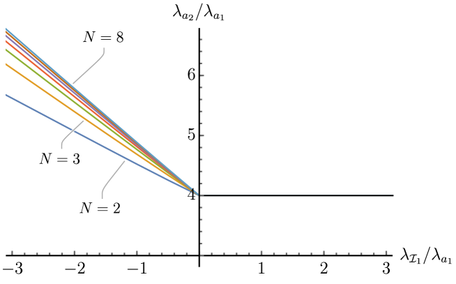
A simplifying feature of this problem is that the consistency conditions depend only on the two ratios λa2/λa1subscript𝜆subscript𝑎2subscript𝜆subscript𝑎1\lambda_{a_{2}}/\lambda_{a_{1}} and λ1/λa1subscript𝜆subscript1subscript𝜆subscript𝑎1\lambda_{\mathcal{I}_{1}}/\lambda_{a_{1}}, which ensures that the resulting constraints are independent of constant rescalings of the metric. For each value of λ1/λa1subscript𝜆subscript1subscript𝜆subscript𝑎1\lambda_{\mathcal{I}_{1}}/\lambda_{a_{1}} we solve a series of SDPs to obtain an upper bound on λa2/λa1subscript𝜆subscript𝑎2subscript𝜆subscript𝑎1\lambda_{a_{2}}/\lambda_{a_{1}}. These upper bounds are shown in Figure 1 for N=2,,8𝑁28N=2,\dots,8. When λ1subscript𝜆subscript1\lambda_{\mathcal{I}_{1}} vanishes we find that λa24λa1subscript𝜆subscript𝑎24subscript𝜆subscript𝑎1\lambda_{a_{2}}\leq 4\lambda_{a_{1}}; this a special case of the bound found in Ref. [12] and is saturated by flat tori whose first eigenvalues are identical to those of a circle, which we call “long flat tori.” For λ1>0subscript𝜆subscript10\lambda_{\mathcal{I}_{1}}>0, the upper bounds decrease linearly until λ1=λa1subscript𝜆subscript1subscript𝜆subscript𝑎1\lambda_{\mathcal{I}_{1}}=\lambda_{a_{1}}, at which point they exhibit kinks and thereafter become constant. The upper bounds grow linearly for negative λ1subscript𝜆subscript1\lambda_{\mathcal{I}_{1}}, so we cannot rule out large values for the ratio of the first two nonzero eigenvalues of the scalar Laplacian on manifolds with large negative Lichnerowicz eigenvalues. In the plot we have also marked the points corresponding to long flat tori and the projective spaces Nsuperscript𝑁\mathbb{RP}^{N} for N=3,,8𝑁38N=3,\dots,8 and N/2superscript𝑁2\mathbb{CP}^{N/2} for N=4,6,8𝑁468N=4,6,8 with their standard metrics (there are no transverse traceless tensors on 2superscript2\mathbb{RP}^{2} and 1S2superscript1superscript𝑆2\mathbb{CP}^{1}\approx S^{2}). These projective spaces all fall comfortably below the bounds. It would be interesting to find out if there are manifolds that live at the kinks of this plot, just as nontrivial CFTs often appear at such kinks in the conformal bootstrap.
Refer to caption
Figure 1: Upper bounds on the ratio of the first distinct nonzero eigenvalues of the scalar Laplacian on closed Einstein manifolds with R0𝑅0R\geq 0 and N=2,,8𝑁28N=2,\dots,8 for different values of the smallest Lichnerowicz eigenvalue of transverse traceless tensors. The square and diamond markers correspond to Nsuperscript𝑁\mathbb{RP}^{N} and N/2superscript𝑁2\mathbb{CP}^{N/2} with their standard metrics and the cross corresponds to long flat N𝑁N-tori.

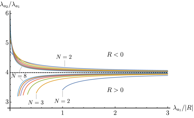
An additional assumption we can make is that the triple overlap integrals ga1a1asubscript𝑔subscript𝑎1subscript𝑎1𝑎g_{a_{1}a_{1}a} vanish when λa=λa1subscript𝜆𝑎subscript𝜆subscript𝑎1\lambda_{a}=\lambda_{a_{1}}, so that the first sum in Eq. (3.3) vanishes. This follows, for example, if there is a 2subscript2\mathbb{Z}_{2} symmetry under which ψa1subscript𝜓subscript𝑎1\psi_{a_{1}} is odd, as is the case for parity on SNsuperscript𝑆𝑁S^{N}. This means that we can drop the constraints in Eq. (3.4d), so it becomes easier to rule out a point and hence the resulting bounds are stronger. We plot these bounds for N=2,,8𝑁28N=2,\dots,8 in Figure 2. As with the previous upper bounds, the trend is an approximately linear decrease until some critical λ1/λa1subscript𝜆subscript1subscript𝜆subscript𝑎1\lambda_{\mathcal{I}_{1}}/\lambda_{a_{1}} is reached, now given by 2(N+1)/N2𝑁1𝑁2(N+1)/N, above which the bound is constant. We also marked the points corresponding to SNsuperscript𝑆𝑁S^{N} for N=3,,8𝑁38N=3,\dots,8, which lie on the boundaries of the allowed regions and away from the kinks. Round spheres thus have the largest possible ratio of the first two distinct nonzero eigenvalues of the scalar Laplacian amongst closed Einstein manifolds with R0𝑅0R\geq 0, a 2subscript2\mathbb{Z}_{2} symmetry, and a sufficiently large value of λ1/λa1subscript𝜆subscript1subscript𝜆subscript𝑎1\lambda_{\mathcal{I}_{1}}/\lambda_{a_{1}}.

Refer to caption
Figure 2: Upper bounds on the ratio of the first distinct nonzero eigenvalues of the scalar Laplacian on closed Einstein manifolds with R0𝑅0R\geq 0 and N=2,,8𝑁28N=2,\dots,8 for different values of the lightest Lichnerowicz eigenvalue, assuming that ga1a1a=0subscript𝑔subscript𝑎1subscript𝑎1𝑎0g_{a_{1}a_{1}a}=0 when λa=λa1subscript𝜆𝑎subscript𝜆subscript𝑎1\lambda_{a}=\lambda_{a_{1}}. The filled circles correspond to round N𝑁N-spheres and the cross corresponds to long flat N𝑁N-tori.

Now let us consider manifolds with either R>0𝑅0R>0 or R<0𝑅0R<0. In these cases we can use the rescaling freedom to set R=±1𝑅plus-or-minus1R=\pm 1 when computing bounds. For R>0𝑅0R>0, the bounds are stronger compared to the R0𝑅0R\geq 0 bounds we considered previously, but the price we pay is the introduction of an additional scale in the problem.

In either case, a candidate spectrum is determined by λa1subscript𝜆subscript𝑎1\lambda_{a_{1}}, λa2subscript𝜆subscript𝑎2\lambda_{a_{2}}, and λ1subscript𝜆subscript1\lambda_{\mathcal{I}_{1}}, where for R>0𝑅0R>0 we also ensure consistency with the Lichnerowicz bound (2.6). Given such a spectrum, we try to rule it out by searching for a constant vector α3𝛼superscript3\vec{\alpha}\in\mathbb{R}^{3} such that
αF1=1,𝛼subscript𝐹11\displaystyle\vec{\alpha}\cdot\vec{F}_{1}=1, (3.5a)
αF20,λλ1,formulae-sequence𝛼subscript𝐹20for-allsubscript𝜆subscript𝜆subscript1\displaystyle\vec{\alpha}\cdot\vec{F}_{2}\geq 0,\quad\forall\,\lambda_{\mathcal{I}}\geq\lambda_{\mathcal{I}_{1}}, (3.5b)
α[((N1)λaR)F3+RF4]0,λaλa2,formulae-sequence𝛼delimited-[]𝑁1subscript𝜆𝑎𝑅subscript𝐹3𝑅subscript𝐹40for-allsubscript𝜆𝑎subscript𝜆subscript𝑎2\displaystyle\vec{\alpha}\cdot\left[((N-1)\lambda_{a}-R)\vec{F}_{3}+R\vec{F}_{4}\right]\geq 0,\quad\forall\,\lambda_{a}\geq\lambda_{a_{2}}, (3.5c)
α[((N1)λaR)F3+RF4]|λa=λa10.evaluated-at𝛼delimited-[]𝑁1subscript𝜆𝑎𝑅subscript𝐹3𝑅subscript𝐹4subscript𝜆𝑎subscript𝜆subscript𝑎10\displaystyle\vec{\alpha}\cdot\left[((N-1)\lambda_{a}-R)\vec{F}_{3}+R\vec{F}_{4}\right]\Big{|}_{\lambda_{a}=\lambda_{a_{1}}}\geq 0. (3.5d)

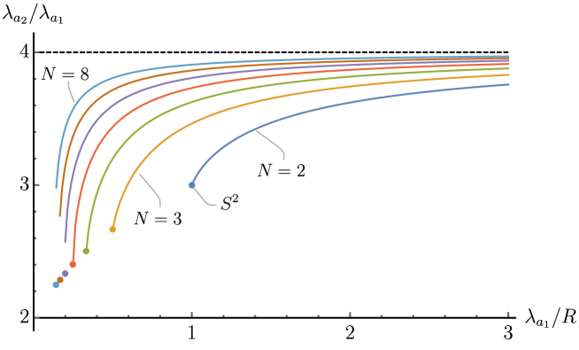
Since we now have an extra scale, we must fix λ1subscript𝜆subscript1\lambda_{\mathcal{I}_{1}} to make a two-dimensional plot of the allowed eigenvalues λa1subscript𝜆subscript𝑎1\lambda_{a_{1}} and λa2subscript𝜆subscript𝑎2\lambda_{a_{2}}. In Figure 3 we show the upper bounds on λa2/λa1subscript𝜆subscript𝑎2subscript𝜆subscript𝑎1\lambda_{a_{2}}/\lambda_{a_{1}} for each value of λa1/|R|subscript𝜆subscript𝑎1𝑅\lambda_{a_{1}}/|R| on closed Einstein manifolds with N=2,,8𝑁28N=2,\dots,8 and R>0𝑅0R>0 or R<0𝑅0R<0, assuming that λ0subscript𝜆0\lambda_{\mathcal{I}}\geq 0. When λa1subscript𝜆subscript𝑎1\lambda_{a_{1}} is of order the curvature scale, the R>0𝑅0R>0 bounds are stronger than what we found above, but they approach the R0𝑅0R\geq 0 bound (the dashed line) as λa1/Rsubscript𝜆subscript𝑎1𝑅\lambda_{a_{1}}/R\rightarrow\infty. Intuitively, this is because the effects of curvature become negligible for high-frequency modes. The bounds for R<0𝑅0R<0 approach λa2/λa1=4subscript𝜆subscript𝑎2subscript𝜆subscript𝑎14\lambda_{a_{2}}/\lambda_{a_{1}}=4 from above.

Refer to caption
Figure 3: Upper bounds on the ratio of the first distinct nonzero eigenvalues of the scalar Laplacian for closed Einstein manifolds with R0𝑅0R\neq 0 and N=2,,8𝑁28N=2,\dots,8, assuming that λ0subscript𝜆0\lambda_{\mathcal{I}}\geq 0. The minimum eigenvalues for R>0𝑅0R>0 are set by the Lichnerowicz bound (2.6).

We now show how the bounds change if we make a stronger assumption about the size of the first Lichnerowicz eigenvalue. In Figure 4 we show the bounds on λa2/λa1subscript𝜆subscript𝑎2subscript𝜆subscript𝑎1\lambda_{a_{2}}/\lambda_{a_{1}} for closed Einstein manifolds with R>0𝑅0R>0 and N=2,,8𝑁28N=2,\dots,8 when λsubscript𝜆\lambda_{\mathcal{I}} satisfies the inequality in Eq. (2.16), the lower bound implied by the existence of a Killing spinor. We also plot the points corresponding to SNsuperscript𝑆𝑁S^{N}, which saturate the bounds for N=2,,5𝑁25N=2,\dots,5 but not for N=6,7,8𝑁678N=6,7,8 (they would if we made the stronger assumption that λ4R/(N1)subscript𝜆4𝑅𝑁1\lambda_{\mathcal{I}}\geq 4R/(N-1)).

Refer to caption
Figure 4: Upper bounds on the ratio of the first distinct nonzero eigenvalues of the scalar Laplacian for closed Einstein manifolds with R>0𝑅0R>0 and N=2,,8𝑁28N=2,\dots,8, assuming that the Lichnerowicz eigenvalues satisfy Eq. (2.16). These bounds apply to closed Einstein manifolds that admit Killing spinors, such as Einstein–Sasaki manifolds. The filled circles correspond to SNsuperscript𝑆𝑁S^{N}.

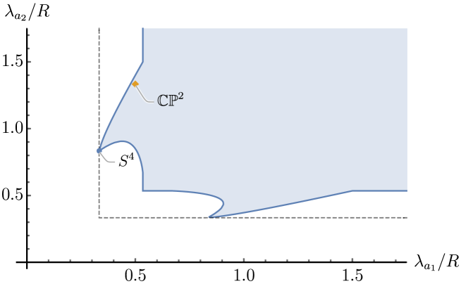
Next we explore a slightly different type of question about eigenvalues. Suppose we assume a particular value for the third nonzero scalar eigenvalue and ask what values the first and second eigenvalues can take. In particular, let us set N=4𝑁4N=4 and assume the following:

λa{λa1,λa2}[3R2,),λ4R3,formulae-sequencesubscript𝜆𝑎subscript𝜆subscript𝑎1subscript𝜆subscript𝑎23𝑅2subscript𝜆4𝑅3\lambda_{a}\in\{\lambda_{a_{1}},\lambda_{a_{2}}\}\cup\left[\frac{3R}{2},\infty\right),\quad\lambda_{\mathcal{I}}\geq\frac{4R}{3}\,, (3.6)

which is consistent with both S4superscript𝑆4S^{4} and 2superscript2\mathbb{CP}^{2} with their standard metrics. With these assumptions, the values of λa1/Rsubscript𝜆subscript𝑎1𝑅\lambda_{a_{1}}/R and λa2/Rsubscript𝜆subscript𝑎2𝑅\lambda_{a_{2}}/R allowed by the consistency conditions (2.28) are given by the blue region in Figure 5. We see that the 4-sphere lives at the tip of a pointed part of the allowed region. To compute these bounds we used two copies of the consistency conditions (2.28), one for λa1subscript𝜆subscript𝑎1\lambda_{a_{1}} and one for λa2subscript𝜆subscript𝑎2\lambda_{a_{2}}. The plot is invariant under a reflection along the diagonal since λa1subscript𝜆subscript𝑎1\lambda_{a_{1}} and λa2subscript𝜆subscript𝑎2\lambda_{a_{2}} are treated symmetrically.

Refer to caption
Figure 5: The blue region shows the allowed values of the two smallest nonzero eigenvalues of the scalar Laplacian on closed four-dimensional Einstein manifolds with R>0𝑅0R>0, assuming the eigenvalues satisfy the conditions in Eq. (3.6). The dashed line is the Lichnerowicz bound and the points corresponding to S4superscript𝑆4S^{4} and 2superscript2\mathbb{CP}^{2} with their standard metrics are marked.

The results so far have been general bounds for all manifolds satisfying a handful of assumptions. We can also try to obtain constraints for specific manifolds by inputting additional information. Suppose that we know the scalar eigenfunctions on a given manifold but not necessarily the Lichnerowicz spectrum. We can then write the consistency conditions as

αF1+1λa12αF2ga1a12=0,𝛼subscriptsuperscript𝐹11superscriptsubscript𝜆subscript𝑎12subscript𝛼subscript𝐹2superscriptsubscript𝑔subscript𝑎1subscript𝑎120\vec{\alpha}\cdot\vec{F}^{\prime}_{1}+\frac{1}{\lambda_{a_{1}}^{2}}\sum_{\mathcal{I}}\vec{\alpha}\cdot\vec{F}_{2}\,g_{a_{1}a_{1}\mathcal{I}}^{2}=0, (3.7)

where F1superscriptsubscript𝐹1\vec{F}_{1}^{\prime} combines the first and third terms of Eq. (3.1) and is assumed to be some known constant vector for a given choice of ψa1subscript𝜓subscript𝑎1\psi_{a_{1}}. We can then find an upper bound on λ1subscript𝜆subscript1\lambda_{\mathcal{I}_{1}}, the smallest Lichnerowicz eigenvalue on transverse traceless tensors, by finding the smallest λ1subscript𝜆subscript1\lambda_{\mathcal{I}_{1}} for which there exists a vector α3𝛼superscript3\vec{\alpha}\in\mathbb{R}^{3} satisfying

αF1=1,𝛼subscriptsuperscript𝐹11\displaystyle\vec{\alpha}\cdot\vec{F}^{\prime}_{1}=1, (3.8)
αF20,λλ1.formulae-sequence𝛼subscript𝐹20for-allsubscript𝜆subscript𝜆subscript1\displaystyle\vec{\alpha}\cdot\vec{F}_{2}\geq 0,\quad\forall\,\lambda_{\mathcal{I}}\geq\lambda_{\mathcal{I}_{1}}. (3.9)

We have carried out this procedure for the compact symmetric spaces of rank one restricted to the subsector of zonal spherical functions (see Appendix A), taking ψa1subscript𝜓subscript𝑎1\psi_{a_{1}} to be the lightest nontrivial zonal spherical function. For these cases, the equations can be solved analytically and therefore the bounds are exact. This gives the following finite bounds for n>1𝑛1n>1:

  • For nsuperscript𝑛\mathbb{CP}^{n} we find λ18(n+2)subscript𝜆subscript18𝑛2\lambda_{\mathcal{I}_{1}}\leq 8(n+2), which is saturated for n=2𝑛2n=2 [33, 34].

  • For nsuperscript𝑛\mathbb{HP}^{n} we find λ18(2n+3)subscript𝜆subscript182𝑛3\lambda_{\mathcal{I}_{1}}\leq 8(2n+3), consistent with the lower bound λ116nsubscript𝜆subscript116𝑛\lambda_{\mathcal{I}_{1}}\geq 16n inferred from Ref. [24].

  • For 𝕆2𝕆superscript2\mathbb{OP}^{2} we find λ126subscript𝜆subscript126\lambda_{\mathcal{I}_{1}}\leq 26, consistent with the lower bound λ116subscript𝜆subscript116\lambda_{\mathcal{I}_{1}}\geq 16 inferred from Ref. [24].

3.1.2 General eigenvalues

The above bounds constrain just the smallest eigenvalues, but we can also look for bounds on general eigenvalues. Let ψa1subscript𝜓subscript𝑎1\psi_{a_{1}} now be a generic eigenfunction of the scalar Laplacian, with eigenvalue λa1subscript𝜆subscript𝑎1\lambda_{a_{1}}, and define λa2subscript𝜆subscript𝑎2\lambda_{a_{2}} as the smallest eigenvalue bigger than λa1subscript𝜆subscript𝑎1\lambda_{a_{1}}, i.e., the scalar eigenvalues satisfy

λa(0,λa1][λa2,),λa1<λa2.formulae-sequencesubscript𝜆𝑎0subscript𝜆subscript𝑎1subscript𝜆subscript𝑎2subscript𝜆subscript𝑎1subscript𝜆subscript𝑎2\lambda_{a}\in(0,\lambda_{a_{1}}]\cup[\lambda_{a_{2}},\infty)\,,\quad\lambda_{a_{1}}<\lambda_{a_{2}}\,. (3.10)

The eigenfunction expansion of ψa12superscriptsubscript𝜓subscript𝑎12\psi_{a_{1}}^{2} can then be written as

ψa12=V1+λaλa1ga1a1ψaa+λaλa2ga1a1ψaa.superscriptsubscript𝜓subscript𝑎12superscript𝑉1subscriptsubscript𝜆𝑎subscript𝜆subscript𝑎1subscript𝑔subscript𝑎1subscript𝑎1superscriptsubscript𝜓𝑎𝑎subscriptsubscript𝜆𝑎subscript𝜆subscript𝑎2subscript𝑔subscript𝑎1subscript𝑎1superscriptsubscript𝜓𝑎𝑎\psi_{a_{1}}^{2}=V^{-1}+\sum_{\begin{subarray}{c}\lambda_{a}\leq\lambda_{a_{1}}\end{subarray}}g_{a_{1}a_{1}}{}^{a}\psi_{a}+\sum_{\begin{subarray}{c}\lambda_{a}\geq\lambda_{a_{2}}\end{subarray}}g_{a_{1}a_{1}}{}^{a}\psi_{a}\,. (3.11)

We again define λ1subscript𝜆subscript1\lambda_{\mathcal{I}_{1}} as the smallest eigenvalue of the Lichnerowicz Laplacian on transverse traceless tensors.

We want to determine how large λa2/λa1subscript𝜆subscript𝑎2subscript𝜆subscript𝑎1\lambda_{a_{2}}/\lambda_{a_{1}} can be for a given choice of λ1/λa1subscript𝜆subscript1subscript𝜆subscript𝑎1\lambda_{\mathcal{I}_{1}}/\lambda_{a_{1}}.

For a closed Einstein manifold with R0𝑅0R\geq 0, we can deduce that a given choice of eigenvalues is not feasible if we can find a constant vector α3𝛼superscript3\vec{\alpha}\in\mathbb{R}^{3} such that
αF1=1,𝛼subscript𝐹11\displaystyle\vec{\alpha}\cdot\vec{F}_{1}=1, (3.12a)
αF20,λλ1,formulae-sequence𝛼subscript𝐹20for-allsubscript𝜆subscript𝜆subscript1\displaystyle\vec{\alpha}\cdot\vec{F}_{2}\geq 0,\quad\forall\,\lambda_{\mathcal{I}}\geq\lambda_{\mathcal{I}_{1}}, (3.12b)
αFk0,k=3,4,λaλa2,formulae-sequence𝛼subscript𝐹𝑘0formulae-sequence𝑘34for-allsubscript𝜆𝑎subscript𝜆subscript𝑎2\displaystyle\vec{\alpha}\cdot\vec{F}_{k}\geq 0,\quad k=3,4,\quad\forall\,\lambda_{a}\geq\lambda_{a_{2}}, (3.12c)
αFk0,k=3,4,λaλa1.formulae-sequence𝛼subscript𝐹𝑘0formulae-sequence𝑘34for-allsubscript𝜆𝑎subscript𝜆subscript𝑎1\displaystyle\vec{\alpha}\cdot\vec{F}_{k}\geq 0,\quad k=3,4,\quad\forall\,\lambda_{a}\leq\lambda_{a_{1}}. (3.12d)

To be able to formulate this last condition as an SDP we can write it as

λa3αFk0,k=3,4,λa=λa1/(1+x),x0.formulae-sequencesuperscriptsubscript𝜆𝑎3𝛼subscript𝐹𝑘0formulae-sequence𝑘34formulae-sequencesubscript𝜆𝑎subscript𝜆subscript𝑎11𝑥for-all𝑥0\lambda_{a}^{-3}\vec{\alpha}\cdot\vec{F}_{k}\geq 0,\quad k=3,4,\quad\lambda_{a}=\lambda_{a_{1}}/(1+x),\quad\forall\,x\geq 0. (3.13)

The resulting upper bounds on λa2/λa1subscript𝜆subscript𝑎2subscript𝜆subscript𝑎1\lambda_{a_{2}}/\lambda_{a_{1}} are shown in Figure 6 for N=2,,8𝑁28N=2,\dots,8. The bounds grow linearly for λ1<0subscript𝜆subscript10\lambda_{\mathcal{I}_{1}}<0 and are constant for λ10subscript𝜆subscript10\lambda_{\mathcal{I}_{1}}\geq 0, given by λa2/λa14subscript𝜆subscript𝑎2subscript𝜆subscript𝑎14\lambda_{a_{2}}/\lambda_{a_{1}}\leq 4 in all dimensions. This result in the case λ1=0subscript𝜆subscript10\lambda_{\mathcal{I}_{1}}=0 was already given in Ref. [12].

Refer to caption
Figure 6: Upper bounds on the ratio of any two consecutive nonzero eigenvalues of the scalar Laplacian for closed Einstein manifolds with R0𝑅0R\geq 0 and N=2,,8𝑁28N=2,\dots,8 for different values of λ1subscript𝜆subscript1\lambda_{\mathcal{I}_{1}}. The bounds for λ10subscript𝜆subscript10\lambda_{\mathcal{I}_{1}}\geq 0, given by the solid black line, are the same for each N𝑁N.

3.2 Bounds on cubic couplings

We have seen that the consistency conditions can be used to derive bounds on Laplacian eigenvalues. Now we show that they can also give upper bounds on the triple overlap integrals of eigenfunctions of Laplacian operators, which correspond to cubic couplings in Kaluza–Klein theories.666It is also possible to find lower bounds in some cases, but we will not discuss these here. These couplings must be real and can take either sign, but we will see that sometimes their absolute values are bounded from above by fixed multiples of geometric invariants.

3.2.1 Spin-2 self-interactions

We start by looking for bounds on the integral of the cube of an eigenfunction of the scalar Laplacian,

ga1a1a1ψa13.subscript𝑔subscript𝑎1subscript𝑎1subscript𝑎1subscriptsuperscriptsubscript𝜓subscript𝑎13g_{a_{1}a_{1}a_{1}}\equiv\int_{\mathcal{M}}\psi_{a_{1}}^{3}. (3.14)

In Kaluza–Klein reductions of GR down to a d𝑑d-dimensional flat spacetime, the massive spin-2 excitations of the graviton in the lower-dimensional theory interact with one another through tree-level cubic amplitudes of the form [12]

𝒜(1ha1, 2ha2, 3ha3)=2Mdd22ga1a2a3V(ϵ1ϵ2ϵ3p1+ϵ2ϵ3ϵ1p2+ϵ1ϵ3ϵ2p3)2,𝒜superscriptsubscript1subscript𝑎1superscriptsubscript2subscript𝑎2superscriptsubscript3subscript𝑎32superscriptsubscript𝑀𝑑𝑑22subscript𝑔subscript𝑎1subscript𝑎2subscript𝑎3𝑉superscriptsubscriptitalic-ϵ1subscriptitalic-ϵ2subscriptitalic-ϵ3subscript𝑝1subscriptitalic-ϵ2subscriptitalic-ϵ3subscriptitalic-ϵ1subscript𝑝2subscriptitalic-ϵ1subscriptitalic-ϵ3subscriptitalic-ϵ2subscript𝑝32\mathcal{A}(1_{h}^{a_{1}},\,2_{h}^{a_{2}},\,3_{h}^{a_{3}})=\frac{2}{M_{d}^{\frac{d-2}{2}}}g_{a_{1}a_{2}a_{3}}\sqrt{V}\left(\epsilon_{1}\!\cdot\!\epsilon_{2}\,\epsilon_{3}\!\cdot\!p_{1}+\epsilon_{2}\!\cdot\!\epsilon_{3}\,\epsilon_{1}\!\cdot\!p_{2}+\epsilon_{1}\!\cdot\!\epsilon_{3}\,\epsilon_{2}\!\cdot\!p_{3}\right)^{2}, (3.15)

where Mdsubscript𝑀𝑑M_{d} is the lower-dimensional Planck mass, pisubscript𝑝𝑖p_{i} are the momenta, and ϵiϵitensor-productsubscriptitalic-ϵ𝑖subscriptitalic-ϵ𝑖\epsilon_{i}\otimes\epsilon_{i} are polarizations. The quantities ga1a2a3Vsubscript𝑔subscript𝑎1subscript𝑎2subscript𝑎3𝑉g_{a_{1}a_{2}a_{3}}\sqrt{V} thus control the strengths of these interactions relative to the strength of gravity. In particular, ga1a1a1Vsubscript𝑔subscript𝑎1subscript𝑎1subscript𝑎1𝑉g_{a_{1}a_{1}a_{1}}\sqrt{V} gives the relative strength of the self-interaction.

We assume that the scalar eigenvalues satisfy

λa{λa1}[λa2,),subscript𝜆𝑎subscript𝜆subscript𝑎1subscript𝜆subscript𝑎2\lambda_{a}\in\{\lambda_{a_{1}}\}\cup[\lambda_{a_{2}},\infty)\,, (3.16)

so that λa2subscript𝜆subscript𝑎2\lambda_{a_{2}} is second smallest nonzero scalar eigenvalue if it is greater than λa1subscript𝜆subscript𝑎1\lambda_{a_{1}}, otherwise it is the smallest nonzero eigenvalue. We again define λ1subscript𝜆subscript1\lambda_{\mathcal{I}_{1}} as the smallest Lichnerowicz eigenvalue on transverse traceless tensors. We want to use the consistency conditions to find an upper bound on |ga1a1a1|Vsubscript𝑔subscript𝑎1subscript𝑎1subscript𝑎1𝑉|g_{a_{1}a_{1}a_{1}}|\sqrt{V} for a given choice of the low-lying eigenvalues λa1subscript𝜆subscript𝑎1\lambda_{a_{1}}, λa2subscript𝜆subscript𝑎2\lambda_{a_{2}}, and λ1subscript𝜆subscript1\lambda_{\mathcal{I}_{1}}. This can be achieved with the same strategy used to bound OPE coefficients in the conformal bootstrap [35]. If R0𝑅0R\geq 0, we look for a vector α3𝛼superscript3\vec{\alpha}\in\mathbb{R}^{3} that satisfies the following constraints:

αF3|λa=λa1=1,evaluated-at𝛼subscript𝐹3subscript𝜆𝑎subscript𝜆subscript𝑎11\displaystyle\vec{\alpha}\cdot\vec{F}_{3}\Big{|}_{\lambda_{a}=\lambda_{a_{1}}}=1, (3.17a)
αF4|λa=λa10,evaluated-at𝛼subscript𝐹4subscript𝜆𝑎subscript𝜆subscript𝑎10\displaystyle\vec{\alpha}\cdot\vec{F}_{4}\Big{|}_{\lambda_{a}=\lambda_{a_{1}}}\geq 0, (3.17b)
αFk0,k=3,4,λaλa2,formulae-sequence𝛼subscript𝐹𝑘0formulae-sequence𝑘34for-allsubscript𝜆𝑎subscript𝜆subscript𝑎2\displaystyle\vec{\alpha}\cdot\vec{F}_{k}\geq 0,\quad k=3,4,\quad\forall\lambda_{a}\geq\lambda_{a_{2}}, (3.17c)
αF20,λλ1.formulae-sequence𝛼subscript𝐹20for-allsubscript𝜆subscript𝜆subscript1\displaystyle\vec{\alpha}\cdot\vec{F}_{2}\geq 0,\quad\forall\lambda_{\mathcal{I}}\geq\lambda_{\mathcal{I}_{1}}. (3.17d)

Rearranging Eq. (3.1) and using these constraints, we get

Vλa=λa1ga1a1a2αF1|ga1a1a1|VαF1,𝑉subscriptsubscript𝜆𝑎subscript𝜆subscript𝑎1subscriptsuperscript𝑔2subscript𝑎1subscript𝑎1𝑎𝛼subscript𝐹1subscript𝑔subscript𝑎1subscript𝑎1subscript𝑎1𝑉𝛼subscript𝐹1V\sum_{\lambda_{a}=\lambda_{a_{1}}}g^{2}_{a_{1}a_{1}a}\leq-\vec{\alpha}\cdot\vec{F}_{1}\implies|g_{a_{1}a_{1}a_{1}}|\sqrt{V}\leq\sqrt{-\vec{\alpha}\cdot\vec{F}_{1}}, (3.18)

i.e., an upper bound on the rescaling invariant combination |ga1a1a1|Vsubscript𝑔subscript𝑎1subscript𝑎1subscript𝑎1𝑉|g_{a_{1}a_{1}a_{1}}|\sqrt{V}. For simplicity we use the second inequality in Eq. (3.18), although the first inequality is stronger when λa1subscript𝜆subscript𝑎1\lambda_{a_{1}} is degenerate. To find the best upper bound, we search for an α𝛼\vec{\alpha} that maximizes the objective function αF1𝛼subscript𝐹1\vec{\alpha}\cdot\vec{F}_{1} while satisfying the constraints in Eqs. (3.17). This is again a problem that can be formulated as an SDP [29]. This SDP, and all others in the remainder of this section, are simple enough that they can be solved analytically using the Minimize function in Mathematica.

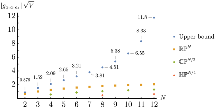
We start by searching for a bound on |ga1a1a1|Vsubscript𝑔subscript𝑎1subscript𝑎1subscript𝑎1𝑉|g_{a_{1}a_{1}a_{1}}|\sqrt{V} with λa2=λa1subscript𝜆subscript𝑎2subscript𝜆subscript𝑎1\lambda_{a_{2}}=\lambda_{a_{1}}, i.e., assuming only that the nonzero scalar eigenvalues satisfy λaλa1subscript𝜆𝑎subscript𝜆subscript𝑎1\lambda_{a}\geq\lambda_{a_{1}}. We also assume for now that λ0subscript𝜆0\lambda_{\mathcal{I}}\geq 0. With these assumptions, we find finite upper bounds on |ga1a1a1|Vsubscript𝑔subscript𝑎1subscript𝑎1subscript𝑎1𝑉|g_{a_{1}a_{1}a_{1}}|\sqrt{V} for N13𝑁13N\leq 13. These bounds are independent of λa1subscript𝜆subscript𝑎1\lambda_{a_{1}}, as required by rescaling invariance. We plot the bounds together with their rounded numerical values for N12𝑁12N\leq 12 in Figure 7. For N=13𝑁13N=13 the upper bound is 28.5absent28.5\approx 28.5. The exact bounds are algebraic numbers, such as 16/1111611116/\sqrt{111} for N=3𝑁3N=3, but mostly their exact forms are not very enlightening. We also mark the points corresponding to the lightest nontrivial zonal spherical functions on the projective spaces Nsuperscript𝑁\mathbb{RP}^{N}, N/2superscript𝑁2\mathbb{CP}^{N/2}, and N/4superscript𝑁4\mathbb{HP}^{N/4} with their standard metrics. The overlap integrals of these eigenfunctions can be calculated by integrating products of Jacobi polynomials, as described in Appendix A. The upper bound increases with N𝑁N, so for manifolds satisfying our assumptions we can get a lower bound on the number of extra dimensions if we know the strength of the cubic self-interaction of the lightest Kaluza–Klein state relative to the strength of gravity.
Refer to caption
Figure 7: Upper bounds on |ga1a1a1|Vsubscript𝑔subscript𝑎1subscript𝑎1subscript𝑎1𝑉|g_{a_{1}a_{1}a_{1}}|\sqrt{V} for closed Einstein manifolds with R0𝑅0R\geq 0 and N=2,,12𝑁212N=2,\dots,12, assuming that λaλa1subscript𝜆𝑎subscript𝜆subscript𝑎1\lambda_{a}\geq\lambda_{a_{1}} and λ0subscript𝜆0\lambda_{\mathcal{I}}\geq 0. The square, diamond, and triangular markers correspond to the lightest nontrivial zonal spherical functions on Nsuperscript𝑁\mathbb{RP}^{N}, N/2superscript𝑁2\mathbb{CP}^{N/2}, and N/4superscript𝑁4\mathbb{HP}^{N/4}, respectively, with their standard metrics.

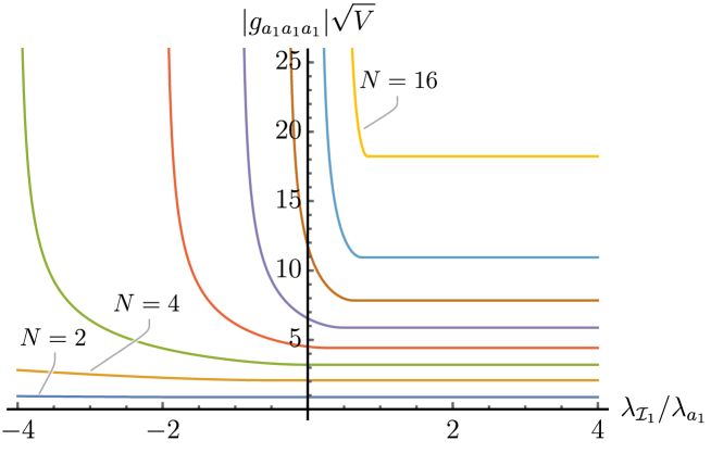
We now generalize the upper bounds on |ga1a1a1|Vsubscript𝑔subscript𝑎1subscript𝑎1subscript𝑎1𝑉|g_{a_{1}a_{1}a_{1}}|\sqrt{V} to allow for different values of λ1/λa1subscript𝜆subscript1subscript𝜆subscript𝑎1\lambda_{\mathcal{I}_{1}}/\lambda_{a_{1}}. These are shown in Figure 8 for N=2,4,,16𝑁2416N=2,4,\dots,16, where the restriction to even N𝑁N is just to keep the plots readable. The intercepts of the curves with the vertical axis give the bounds of Figure 7. There exists a finite upper bound when N17𝑁17N\leq 17 and λ1/λa1>wNsubscript𝜆subscript1subscript𝜆subscript𝑎1subscript𝑤𝑁\lambda_{\mathcal{I}_{1}}/\lambda_{a_{1}}>w_{N}, where wNsubscript𝑤𝑁w_{N} is a finite constant. The first few of these constants are w2=(38+166)subscript𝑤238166w_{2}=-(38+16\sqrt{6}), w319.380subscript𝑤319.380w_{3}\approx-19.380, w49.7272subscript𝑤49.7272w_{4}\approx-9.7272, w55.9714subscript𝑤55.9714w_{5}\approx-5.9714, and w6=4subscript𝑤64w_{6}=-4, where the two exact expressions hold to at least 16-digit precision. For large enough values of λ1/λa1subscript𝜆subscript1subscript𝜆subscript𝑎1\lambda_{\mathcal{I}_{1}}/\lambda_{a_{1}}, the bounds become constant.

Refer to caption
Figure 8: Upper bounds on |ga1a1a1|Vsubscript𝑔subscript𝑎1subscript𝑎1subscript𝑎1𝑉|g_{a_{1}a_{1}a_{1}}|\sqrt{V} as a function of λ1/λa1subscript𝜆subscript1subscript𝜆subscript𝑎1\lambda_{\mathcal{I}_{1}}/\lambda_{a_{1}} for closed Einstein manifolds with R0𝑅0R\geq 0 and N=2,4,,16𝑁2416N=2,4,\dots,16, assuming that λaλa1subscript𝜆𝑎subscript𝜆subscript𝑎1\lambda_{a}\geq\lambda_{a_{1}} and λλ1subscript𝜆subscript𝜆subscript1\lambda_{\mathcal{I}}\geq\lambda_{\mathcal{I}_{1}}.

Next we explore the effect of varying λa2/λa1subscript𝜆subscript𝑎2subscript𝜆subscript𝑎1\lambda_{a_{2}}/\lambda_{a_{1}}, assuming again that λ0subscript𝜆0\lambda_{\mathcal{I}}\geq 0. In Figure 9 we plot the resulting bounds for λa2/λa1(0,4]subscript𝜆subscript𝑎2subscript𝜆subscript𝑎104\lambda_{a_{2}}/\lambda_{a_{1}}\in(0,4] for manifolds with R0𝑅0R\geq 0 and N=2,4,,10𝑁2410N=2,4,\dots,10. When λa2/λa1=1subscript𝜆subscript𝑎2subscript𝜆subscript𝑎11\lambda_{a_{2}}/\lambda_{a_{1}}=1, we recover the bounds of Figure 7. When λa2/λa1=4subscript𝜆subscript𝑎2subscript𝜆subscript𝑎14\lambda_{a_{2}}/\lambda_{a_{1}}=4, which is the maximum possible value and is achieved by long flat tori, we find that the self-coupling must vanish. This is consistent with the vanishing of all self-couplings on flat tori, which follows from their U(1)N𝑈superscript1𝑁U(1)^{N} symmetry. The eigenfunction ψa1subscript𝜓subscript𝑎1\psi_{a_{1}} becomes completely general in the limit λa2/λa10subscript𝜆subscript𝑎2subscript𝜆subscript𝑎10\lambda_{a_{2}}/\lambda_{a_{1}}\rightarrow 0, so it is not surprising that in this limit there is no finite bound for N>2𝑁2N>2. More precisely, a finite bound exists for λa2/λa1>xNsubscript𝜆subscript𝑎2subscript𝜆subscript𝑎1subscript𝑥𝑁\lambda_{a_{2}}/\lambda_{a_{1}}>x_{N}, where xNsubscript𝑥𝑁x_{N} is a constant that is positive for N>2𝑁2N>2. For N13𝑁13N\leq 13 the bounds approach a finite value as λa2/λa1xN+subscript𝜆subscript𝑎2subscript𝜆subscript𝑎1superscriptsubscript𝑥𝑁\lambda_{a_{2}}/\lambda_{a_{1}}\rightarrow x_{N}^{+}, so to high numerical precision they appear to be discontinuous at these points. It would be interesting if there is an explanation for this in terms of explicit manifolds. We list numerical approximations to xNsubscript𝑥𝑁x_{N} for N=2,,14𝑁214N=2,\dots,14 and the corresponding bounds in Table 2. To at least 151515-digit precision we have x3=12/(15+230)subscript𝑥31215230x_{3}=12/(15+2\sqrt{30}), x4=(16624)/106subscript𝑥416624106x_{4}=(16\sqrt{6}-24)/10\sqrt{6}, and x14=12/5subscript𝑥14125x_{14}=12/5.

N𝑁N xNsubscript𝑥𝑁x_{N} |ga1a1a1|Vsubscript𝑔subscript𝑎1subscript𝑎1subscript𝑎1𝑉|g_{a_{1}a_{1}a_{1}}|\sqrt{V}
 2 0 22/30.942812230.942812\sqrt{2}/3\approx 0.94281
3 0.46235 1.5187
4 0.62020 2.1094
5 0.70941 2.6671
6 0.77426 3.2109
7 0.82514 3.8127
8 0.86641 4.5146
9 0.90072 5.3844
10 0.92980 6.5524
11 0.95483 8.3291
12 0.97666 11.781
13 0.99588 28.459
14 2.4000 \infty
Table 2: Upper bounds on the size of the cubic self-coupling |ga1a1a1|Vsubscript𝑔subscript𝑎1subscript𝑎1subscript𝑎1𝑉|g_{a_{1}a_{1}a_{1}}|\sqrt{V} for closed Einstein manifolds with R0𝑅0R\geq 0 and λ0subscript𝜆0\lambda_{\mathcal{I}}\geq 0 as λa2/λa1xN+subscript𝜆subscript𝑎2subscript𝜆subscript𝑎1superscriptsubscript𝑥𝑁\lambda_{a_{2}}/\lambda_{a_{1}}\rightarrow x_{N}^{+}, where λa{λa1}[λa2,)subscript𝜆𝑎subscript𝜆subscript𝑎1subscript𝜆subscript𝑎2\lambda_{a}\in\{\lambda_{a_{1}}\}\cup[\lambda_{a_{2}},\infty) and xNsubscript𝑥𝑁x_{N} is the smallest value of λa2/λa1subscript𝜆subscript𝑎2subscript𝜆subscript𝑎1\lambda_{a_{2}}/\lambda_{a_{1}} below which there is no finite bound.
Refer to captionx4subscript𝑥4x_{4}
Figure 9: Upper bounds on |ga1a1a1|Vsubscript𝑔subscript𝑎1subscript𝑎1subscript𝑎1𝑉|g_{a_{1}a_{1}a_{1}}|\sqrt{V} for closed Einstein manifolds with R0𝑅0R\geq 0 and N=2,4,,20𝑁2420N=2,4,\dots,20, assuming that λ0subscript𝜆0\lambda_{\mathcal{I}}\geq 0 and λa{λa1}[λa2,)subscript𝜆𝑎subscript𝜆subscript𝑎1subscript𝜆subscript𝑎2\lambda_{a}\in\{\lambda_{a_{1}}\}\cup[\lambda_{a_{2}},\infty).

3.2.2 Interactions with multiple spin-2 fields

We now look for bounds on triple overlap integrals of the form

ga1a1a2ψa12ψa2.subscript𝑔subscript𝑎1subscript𝑎1subscript𝑎2subscriptsuperscriptsubscript𝜓subscript𝑎12subscript𝜓subscript𝑎2g_{a_{1}a_{1}a_{2}}\equiv\int_{\mathcal{M}}\psi_{a_{1}}^{2}\psi_{a_{2}}. (3.19)

In Kaluza–Klein reductions of gravity, these integrals give the strengths of the tree-level cubic interactions between two spin-2 particles of different masses.

We assume again that R0𝑅0R\geq 0 and that the scalar eigenvalues satisfy Eq. (3.16). The procedure is similar to before. We choose the vector α3𝛼superscript3\vec{\alpha}\in\mathbb{R}^{3} to satisfy the following constraints:

αF3|λa=λa2=1,evaluated-at𝛼subscript𝐹3subscript𝜆𝑎subscript𝜆subscript𝑎21\displaystyle\vec{\alpha}\cdot\vec{F}_{3}\Big{|}_{\lambda_{a}=\lambda_{a_{2}}}=1, (3.20a)
αF20,λλ1,formulae-sequence𝛼subscript𝐹20for-allsubscript𝜆subscript𝜆subscript1\displaystyle\vec{\alpha}\cdot\vec{F}_{2}\geq 0,\quad\forall\lambda_{\mathcal{I}}\geq\lambda_{\mathcal{I}_{1}}, (3.20b)
αFk|λa=λa10,k=3,4,formulae-sequenceevaluated-at𝛼subscript𝐹𝑘subscript𝜆𝑎subscript𝜆subscript𝑎10𝑘34\displaystyle\vec{\alpha}\cdot\vec{F}_{k}\Big{|}_{\lambda_{a}=\lambda_{a_{1}}}\geq 0,\quad k=3,4, (3.20c)
αFk0,k=3,4,λaλa2.formulae-sequence𝛼subscript𝐹𝑘0formulae-sequence𝑘34for-allsubscript𝜆𝑎subscript𝜆subscript𝑎2\displaystyle\vec{\alpha}\cdot\vec{F}_{k}\geq 0,\quad k=3,4,\quad\forall\lambda_{a}\geq\lambda_{a_{2}}. (3.20d)

With these constraints satisfied, we search for an α3𝛼superscript3\vec{\alpha}\in\mathbb{R}^{3} that maximizes the objective function αF1𝛼subscript𝐹1\vec{\alpha}\cdot\vec{F}_{1}, giving the bound

Vλa=λa2ga1a1a2αF1|ga1a1a2|VαF1.𝑉subscriptsubscript𝜆𝑎subscript𝜆subscript𝑎2subscriptsuperscript𝑔2subscript𝑎1subscript𝑎1𝑎𝛼subscript𝐹1subscript𝑔subscript𝑎1subscript𝑎1subscript𝑎2𝑉𝛼subscript𝐹1V\sum_{\lambda_{a}=\lambda_{a_{2}}}g^{2}_{a_{1}a_{1}a}\leq-\vec{\alpha}\cdot\vec{F}_{1}\implies|g_{a_{1}a_{1}a_{2}}|\sqrt{V}\leq\sqrt{-\vec{\alpha}\cdot\vec{F}_{1}}. (3.21)

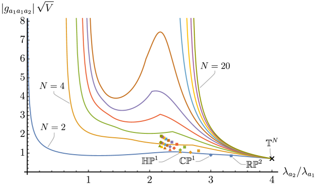
Taking λ0subscript𝜆0\lambda_{\mathcal{I}}\geq 0 gives the bounds shown in Figure 10 for λa2/λa1(0,4]subscript𝜆subscript𝑎2subscript𝜆subscript𝑎104\lambda_{a_{2}}/\lambda_{a_{1}}\in(0,4] and N=2,4,,20𝑁2420N=2,4,\dots,20. The upper bounds do not decrease monotonically as we increase λa2/λa1subscript𝜆subscript𝑎2subscript𝜆subscript𝑎1\lambda_{a_{2}}/\lambda_{a_{1}}, unlike the previous bound. This is possible due to the fact that the normalization condition in Eq. (3.20a) depends on λa2subscript𝜆subscript𝑎2\lambda_{a_{2}}, so a solution α𝛼\vec{\alpha} for some λa2subscript𝜆subscript𝑎2\lambda_{a_{2}} is not necessarily a solution for larger λa2subscript𝜆subscript𝑎2\lambda_{a_{2}}. The bounds all approach 1/2121/\sqrt{2} as λa2/λa14subscript𝜆subscript𝑎2subscript𝜆subscript𝑎14\lambda_{a_{2}}/\lambda_{a_{1}}\rightarrow 4, which is the value attained by long flat tori and is marked with a cross in the plot. The bounds diverge for λa2/λa1<xNsubscript𝜆subscript𝑎2subscript𝜆subscript𝑎1subscript𝑥𝑁\lambda_{a_{2}}/\lambda_{a_{1}}<x_{N}, where xNsubscript𝑥𝑁x_{N} are the constants encountered above. We also mark the points corresponding to the overlap of the two lightest nontrivial zonal spherical functions on Nsuperscript𝑁\mathbb{RP}^{N}, N/2superscript𝑁2\mathbb{CP}^{N/2}, and N/4superscript𝑁4\mathbb{HP}^{N/4} with their standard metrics.

Refer to caption
Figure 10: Upper bounds on the size of the cubic coupling |ga1a1a2|Vsubscript𝑔subscript𝑎1subscript𝑎1subscript𝑎2𝑉|g_{a_{1}a_{1}a_{2}}|\sqrt{V} for closed Einstein manifolds with R0𝑅0R\geq 0 and N=2,4,,20𝑁2420N=2,4,\dots,20 as we vary λa2/λa1subscript𝜆subscript𝑎2subscript𝜆subscript𝑎1\lambda_{a_{2}}/\lambda_{a_{1}}, where λa{λa1}[λa2,)subscript𝜆𝑎subscript𝜆subscript𝑎1subscript𝜆subscript𝑎2\lambda_{a}\in\{\lambda_{a_{1}}\}\cup[\lambda_{a_{2}},\infty) and λ0subscript𝜆0\lambda_{\mathcal{I}}\geq 0. The cross corresponds to the lightest nontrivial modes on long flat N𝑁N-tori. The square, diamond, and triangular markers correspond to the lightest nontrivial zonal spherical functions on Nsuperscript𝑁\mathbb{RP}^{N}, N/2superscript𝑁2\mathbb{CP}^{N/2}, and N/4superscript𝑁4\mathbb{HP}^{N/4} with their standard metrics.

We can get stronger bounds by further imposing that ga1a1asubscript𝑔subscript𝑎1subscript𝑎1𝑎g_{a_{1}a_{1}a} vanishes if λa=λa1subscript𝜆𝑎subscript𝜆subscript𝑎1\lambda_{a}=\lambda_{a_{1}}. This is the case when the eigenfunctions with eigenvalue λa1subscript𝜆subscript𝑎1\lambda_{a_{1}} are odd under a 2subscript2\mathbb{Z}_{2} symmetry. Suppose also that the eigenfunctions with eigenvalue λa2subscript𝜆subscript𝑎2\lambda_{a_{2}} are even, so the eigenvalues of the scalar Laplacian satisfy

λa[λa1,),λa+[λa2,),formulae-sequencesuperscriptsubscript𝜆𝑎subscript𝜆subscript𝑎1superscriptsubscript𝜆𝑎subscript𝜆subscript𝑎2\lambda_{a}^{-}\in[\lambda_{a_{1}},\infty),\quad\lambda_{a}^{+}\in[\lambda_{a_{2}},\infty), (3.22)

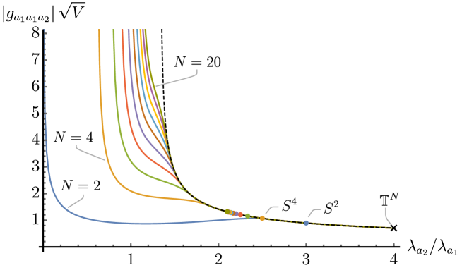
where λa±subscriptsuperscript𝜆plus-or-minus𝑎\lambda^{\pm}_{a} are the nonzero eigenvalues of the even/odd eigenfunctions. We implement this by dropping condition (3.20c). The resulting bounds are shown in Figure 11 for N=2,4,,20𝑁2420N=2,4,\dots,20. We also mark the points corresponding to the overlap of the lightest nontrivial zonal spherical harmonics on SNsuperscript𝑆𝑁S^{N}, which lie on the boundaries of the allowed regions.
Refer to caption
Figure 11: Upper bounds on |ga1a1a2|Vsubscript𝑔subscript𝑎1subscript𝑎1subscript𝑎2𝑉|g_{a_{1}a_{1}a_{2}}|\sqrt{V} as we vary λa2/λa1subscript𝜆subscript𝑎2subscript𝜆subscript𝑎1\lambda_{a_{2}}/\lambda_{a_{1}} for closed Einstein manifolds with R0𝑅0R\geq 0 and a 2subscript2\mathbb{Z}_{2} symmetry, assuming that λ0subscript𝜆0\lambda_{\mathcal{I}}\geq 0, λaλa1superscriptsubscript𝜆𝑎subscript𝜆subscript𝑎1\lambda_{a}^{-}\geq\lambda_{a_{1}}, and λa+λa2superscriptsubscript𝜆𝑎subscript𝜆subscript𝑎2\lambda_{a}^{+}\geq\lambda_{a_{2}}. The cross again corresponds to modes on long flat tori. The filled circles correspond to the overlaps of the lightest nontrivial zonal spherical harmonics on SNsuperscript𝑆𝑁S^{N}. The dashed line is 2(3λa2/λa14)1/22superscript3subscript𝜆subscript𝑎2subscript𝜆subscript𝑎14122(3\lambda_{a_{2}}/\lambda_{a_{1}}-4)^{-1/2}, which the bounds approach as N𝑁N\rightarrow\infty. This plot is identical to Figure 10 in the region λa2/λa11subscript𝜆subscript𝑎2subscript𝜆subscript𝑎11\lambda_{a_{2}}/\lambda_{a_{1}}\leq 1.

3.2.3 Spin-2 and scalar interactions

We now look for bounds on triple overlap integrals involving an eigenfunction of the scalar Laplacian and a transverse traceless eigentensor of the Lichnerowicz Laplacian,

ga1a1mψa1nψa1hmn,TT.subscript𝑔subscript𝑎1subscript𝑎1subscriptsuperscript𝑚subscript𝜓subscript𝑎1superscript𝑛subscript𝜓subscript𝑎1superscriptsubscript𝑚𝑛𝑇𝑇g_{a_{1}a_{1}\mathcal{I}}\equiv\int_{\mathcal{M}}\partial^{m}\psi_{a_{1}}\partial^{n}\psi_{a_{1}}h_{mn,\mathcal{I}}^{TT}. (3.23)

In Kaluza–Klein reductions of gravity, these integrals control the strengths of the cubic interactions between a massive spin-2 mode and a spin-0 Lichnerowicz mode.

We look for bounds involving the lightest eigentensor, hmn,1TTsuperscriptsubscript𝑚𝑛subscript1𝑇𝑇h_{mn,\mathcal{I}_{1}}^{TT}. We assume that λa{λa1}[λa2,)subscript𝜆𝑎subscript𝜆subscript𝑎1subscript𝜆subscript𝑎2\lambda_{a}\in\{\lambda_{a_{1}}\}\cup[\lambda_{a_{2}},\infty). For the case R0𝑅0R\geq 0, we require the vector α3𝛼superscript3\vec{\alpha}\in\mathbb{R}^{3} to satisfy the following constraints:
αF2|λ=λ1=1,evaluated-at𝛼subscript𝐹2subscript𝜆subscript𝜆subscript11\displaystyle\vec{\alpha}\cdot\vec{F}_{2}\Big{|}_{\lambda_{\mathcal{I}}=\lambda_{\mathcal{I}_{1}}}=1, (3.24a)
αFk|λa=λa10,k=3,4,formulae-sequenceevaluated-at𝛼subscript𝐹𝑘subscript𝜆𝑎subscript𝜆subscript𝑎10𝑘34\displaystyle\vec{\alpha}\cdot\vec{F}_{k}\Big{|}_{\lambda_{a}=\lambda_{a_{1}}}\geq 0,\quad k=3,4, (3.24b)
αFk0,k=3,4,λaλa2,formulae-sequence𝛼subscript𝐹𝑘0formulae-sequence𝑘34for-allsubscript𝜆𝑎subscript𝜆subscript𝑎2\displaystyle\vec{\alpha}\cdot\vec{F}_{k}\geq 0,\quad k=3,4,\quad\forall\lambda_{a}\geq\lambda_{a_{2}}, (3.24c)
αF20,λλ1.formulae-sequence𝛼subscript𝐹20for-allsubscript𝜆subscript𝜆subscript1\displaystyle\vec{\alpha}\cdot\vec{F}_{2}\geq 0,\quad\forall\lambda_{\mathcal{I}}\geq\lambda_{\mathcal{I}_{1}}. (3.24d)

This then gives the inequality

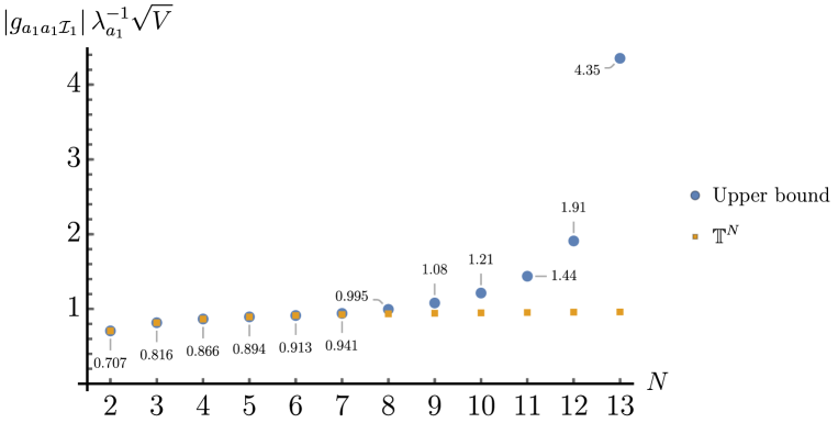
Vλa12λ=λ1ga1a112αF1|ga1a11|λa11VαF1.𝑉superscriptsubscript𝜆subscript𝑎12subscriptsubscript𝜆subscript𝜆subscript1subscriptsuperscript𝑔2subscript𝑎1subscript𝑎1subscript1𝛼subscript𝐹1subscript𝑔subscript𝑎1subscript𝑎1subscript1superscriptsubscript𝜆subscript𝑎11𝑉𝛼subscript𝐹1V\lambda_{a_{1}}^{-2}\sum_{\lambda_{\mathcal{I}}=\lambda_{\mathcal{I}_{1}}}g^{2}_{a_{1}a_{1}\mathcal{I}_{1}}\leq-\vec{\alpha}\cdot\vec{F}_{1}\implies|g_{a_{1}a_{1}\mathcal{I}_{1}}|\lambda_{a_{1}}^{-1}\sqrt{V}\leq\sqrt{-\vec{\alpha}\cdot\vec{F}_{1}}. (3.25)

Maximizing the objective function αF1𝛼subscript𝐹1\vec{\alpha}\cdot\vec{F}_{1} subject to the above constraints then gives the best upper bound on the combination |ga1a11|λa11Vsubscript𝑔subscript𝑎1subscript𝑎1subscript1superscriptsubscript𝜆subscript𝑎11𝑉|g_{a_{1}a_{1}\mathcal{I}_{1}}|\lambda_{a_{1}}^{-1}\sqrt{V}.

The simplest case to consider is λ1=0subscript𝜆subscript10\lambda_{\mathcal{I}_{1}}=0 and λa2=λa1subscript𝜆subscript𝑎2subscript𝜆subscript𝑎1\lambda_{a_{2}}=\lambda_{a_{1}}, so we have λ0subscript𝜆0\lambda_{\mathcal{I}}\geq 0 and λaλa1subscript𝜆𝑎subscript𝜆subscript𝑎1\lambda_{a}\geq\lambda_{a_{1}}. This is relevant, for example, to Ricci-flat manifolds with shape moduli and a parallel spinor. The resulting upper bounds are finite for N13𝑁13N\leq 13 and are shown in Figure 12. We also plot the couplings for certain modes on flat N𝑁N-tori,777For example, on the square flat N𝑁N-torus we can take ψa1=2cosθN(2π)N,hmn,1TT=diag(1,,1,1N)(2π)NN(N1),formulae-sequencesubscript𝜓subscript𝑎12subscript𝜃𝑁superscript2𝜋𝑁superscriptsubscript𝑚𝑛subscript1𝑇𝑇diag111𝑁superscript2𝜋𝑁𝑁𝑁1\psi_{a_{1}}=\frac{\sqrt{2}\cos\theta_{N}}{(\sqrt{2\pi})^{N}},\quad h_{mn,\mathcal{I}_{1}}^{TT}=\frac{{\rm diag}(1,\dots,1,1-N)}{\sqrt{(2\pi)^{N}N(N-1)}}, (3.26) where θk[0,2π)subscript𝜃𝑘02𝜋\theta_{k}\in[0,2\pi) parameterizes the k𝑘kth circle in (S1)Nsuperscriptsuperscript𝑆1𝑁(S^{1})^{N}. By elongating the N𝑁Nth circle we get λa2=4λa1subscript𝜆subscript𝑎24subscript𝜆subscript𝑎1\lambda_{a_{2}}=4\lambda_{a_{1}}.

|ga1a11|λa11V=11N.subscript𝑔subscript𝑎1subscript𝑎1subscript1superscriptsubscript𝜆subscript𝑎11𝑉11𝑁|g_{a_{1}a_{1}\mathcal{I}_{1}}|\lambda_{a_{1}}^{-1}\sqrt{V}=\sqrt{1-\frac{1}{N}}. (3.27)

Interestingly, these tori modes saturate the upper bounds for N=2,,6𝑁26N=2,\dots,6, but not for N7𝑁7N\geq 7. The bounds do not change if we assume instead that R=0𝑅0R=0.

Refer to caption
Figure 12: Upper bounds on |ga1a11|λa11Vsubscript𝑔subscript𝑎1subscript𝑎1subscript1superscriptsubscript𝜆subscript𝑎11𝑉|g_{a_{1}a_{1}\mathcal{I}_{1}}|\lambda_{a_{1}}^{-1}\sqrt{V} for closed Einstein manifolds with R0𝑅0R\geq 0 and N=2,,13𝑁213N=2,\dots,13, where λ1=0subscript𝜆subscript10\lambda_{\mathcal{I}_{1}}=0 and λaλa1subscript𝜆𝑎subscript𝜆subscript𝑎1\lambda_{a}\geq\lambda_{a_{1}}. Some values for flat N𝑁N-tori are also plotted.

We can also find bounds when we vary λa2/λa1subscript𝜆subscript𝑎2subscript𝜆subscript𝑎1\lambda_{a_{2}}/\lambda_{a_{1}}, keeping λ1subscript𝜆subscript1\lambda_{\mathcal{I}_{1}} fixed at zero. We show these in Figure 13 for N=2,4,,20𝑁2420N=2,4,\dots,20. We also mark the points corresponding to the maximum couplings on flat N𝑁N-tori given by Eq. (3.27) at λa2/λa1=4subscript𝜆subscript𝑎2subscript𝜆subscript𝑎14\lambda_{a_{2}}/\lambda_{a_{1}}=4, which saturate the bounds for every N𝑁N. A finite bound exists for λa2/λa1>xNsubscript𝜆subscript𝑎2subscript𝜆subscript𝑎1subscript𝑥𝑁\lambda_{a_{2}}/\lambda_{a_{1}}>x_{N}, where xNsubscript𝑥𝑁x_{N} are the constants from Section 3.2.1. For N4𝑁4N\leq 4 the bound as λa2/λa1xNsubscript𝜆subscript𝑎2subscript𝜆subscript𝑎1subscript𝑥𝑁\lambda_{a_{2}}/\lambda_{a_{1}}\rightarrow x_{N} is finite, given by 1/2121/\sqrt{2}, 1.0491absent1.0491\approx 1.0491, or 1.9773absent1.9773\approx 1.9773 for N=2,3,𝑁23N=2,3, or 4, respectively.

Refer to captionx4subscript𝑥4x_{4}
Figure 13: Upper bounds on |ga1a11|λa11Vsubscript𝑔subscript𝑎1subscript𝑎1subscript1superscriptsubscript𝜆subscript𝑎11𝑉|g_{a_{1}a_{1}\mathcal{I}_{1}}|\lambda_{a_{1}}^{-1}\sqrt{V} as we vary λa2/λa1subscript𝜆subscript𝑎2subscript𝜆subscript𝑎1\lambda_{a_{2}}/\lambda_{a_{1}} for closed Einstein manifolds with R0𝑅0R\geq 0, N=2,4,,20𝑁2420N=2,4,\dots,20, and a lightest Lichnerowicz eigentensor with λ1=0subscript𝜆subscript10\lambda_{\mathcal{I}_{1}}=0, where λa{λa1}[λa2,)subscript𝜆𝑎subscript𝜆subscript𝑎1subscript𝜆subscript𝑎2\lambda_{a}\in\{\lambda_{a_{1}}\}\cup[\lambda_{a_{2}},\infty). The crosses at λa2/λa1=4subscript𝜆subscript𝑎2subscript𝜆subscript𝑎14\lambda_{a_{2}}/\lambda_{a_{1}}=4 correspond to modes on long flat N𝑁N-tori.

We can similarly find bounds when we vary λ1/λa1subscript𝜆subscript1subscript𝜆subscript𝑎1\lambda_{\mathcal{I}_{1}}/\lambda_{a_{1}}, assuming that λaλa1subscript𝜆𝑎subscript𝜆subscript𝑎1\lambda_{a}\geq\lambda_{a_{1}}. We show these bounds for closed Einstein manifolds with R0𝑅0R\geq 0 and N=2,4,,16𝑁2416N=2,4,\dots,16 in Figure 14. A finite bound exists when N17𝑁17N\leq 17 and λ1/λa1>wNsubscript𝜆subscript1subscript𝜆subscript𝑎1subscript𝑤𝑁\lambda_{\mathcal{I}_{1}}/\lambda_{a_{1}}>w_{N}, where wNsubscript𝑤𝑁w_{N} are the constants from Section 3.2.1.

Refer to captionRefer to caption
Figure 14: Upper bounds on |ga1a11|λa11Vsubscript𝑔subscript𝑎1subscript𝑎1subscript1superscriptsubscript𝜆subscript𝑎11𝑉|g_{a_{1}a_{1}\mathcal{I}_{1}}|\lambda_{a_{1}}^{-1}\sqrt{V} as we vary λ1/λa1subscript𝜆subscript1subscript𝜆subscript𝑎1\lambda_{\mathcal{I}_{1}}/\lambda_{a_{1}} for closed Einstein manifolds with R0𝑅0R\geq 0 and N=2,4,,16𝑁2416N=2,4,\dots,16, assuming that λaλa1subscript𝜆𝑎subscript𝜆subscript𝑎1\lambda_{a}\geq\lambda_{a_{1}} and λλ1subscript𝜆subscript𝜆subscript1\lambda_{\mathcal{I}}\geq\lambda_{\mathcal{I}_{1}}.

4 Consistency conditions with two fixed eigenfunctions

The consistency conditions we have been studying so far involve one fixed scalar eigenfunction. These correspond to sum rules for the scattering of identical massive spin-2 Kaluza–Klein particles in dimensional reductions of pure GR when R=0𝑅0R=0. We now study bounds obtained from more general consistency conditions involving two different fixed scalar eigenfunctions, which are related to four-point amplitudes with two different Kaluza–Klein external states. These are the analogue of mixed correlator bootstrap equations for CFTs [30].

The consistency conditions involving two fixed scalar eigenfunctions, ψa1subscript𝜓subscript𝑎1\psi_{a_{1}} and ψa2subscript𝜓subscript𝑎2\psi_{a_{2}}, are given explicitly in Appendix B, where we also explain how to derive them. When combined with the earlier consistency conditions, they can be put in the following form:

V1F1+1λa12(ga1a1ga2a2)F2(ga1a1ga2a2)+1λa12F3ga1a22+iIKilling1λi[F4+RF5Nλi2R]ga1a2i2superscript𝑉1subscript𝐹11superscriptsubscript𝜆subscript𝑎12subscriptmatrixsubscript𝑔subscript𝑎1subscript𝑎1subscript𝑔subscript𝑎2subscript𝑎2subscript𝐹2matrixsubscript𝑔subscript𝑎1subscript𝑎1subscript𝑔subscript𝑎2subscript𝑎21superscriptsubscript𝜆subscript𝑎12subscriptsubscript𝐹3superscriptsubscript𝑔subscript𝑎1subscript𝑎22subscript𝑖subscript𝐼Killing1subscript𝜆𝑖delimited-[]subscript𝐹4𝑅subscript𝐹5𝑁subscript𝜆𝑖2𝑅superscriptsubscript𝑔subscript𝑎1subscript𝑎2𝑖2\displaystyle V^{-1}\vec{F}_{1}+\frac{1}{\lambda_{a_{1}}^{2}}\sum_{\mathcal{I}}\begin{pmatrix}g_{a_{1}a_{1}\mathcal{I}}&g_{a_{2}a_{2}\mathcal{I}}\end{pmatrix}\vec{F}_{2}\begin{pmatrix}g_{a_{1}a_{1}\mathcal{I}}\\ g_{a_{2}a_{2}\mathcal{I}}\end{pmatrix}+\frac{1}{\lambda_{a_{1}}^{2}}\sum_{\mathcal{I}}\vec{F}_{3}g_{a_{1}a_{2}\mathcal{I}}^{2}+\sum_{i\notin I_{\rm Killing}}\frac{1}{\lambda_{i}}\left[\vec{F}_{4}+\frac{R\,\vec{F}_{5}}{N\lambda_{i}-2R}\right]g_{a_{1}a_{2}i}^{2}
+1λa1iIKillingF6ga1a2i2+aIconf.(ga1a1aga2a2a)[F7+RF8(N1)λaR](ga1a1aga2a2a)1subscript𝜆subscript𝑎1subscript𝑖subscript𝐼Killingsubscript𝐹6superscriptsubscript𝑔subscript𝑎1subscript𝑎2𝑖2subscript𝑎subscript𝐼confmatrixsubscript𝑔subscript𝑎1subscript𝑎1𝑎subscript𝑔subscript𝑎2subscript𝑎2𝑎delimited-[]subscript𝐹7𝑅subscript𝐹8𝑁1subscript𝜆𝑎𝑅matrixsubscript𝑔subscript𝑎1subscript𝑎1𝑎subscript𝑔subscript𝑎2subscript𝑎2𝑎\displaystyle+\frac{1}{\lambda_{a_{1}}}\sum_{i\in I_{\rm Killing}}\vec{F}_{6}\,g_{a_{1}a_{2}i}^{2}+\sum_{a\notin I_{\rm conf.}}\begin{pmatrix}g_{a_{1}a_{1}a}&g_{a_{2}a_{2}a}\end{pmatrix}\left[\vec{F}_{7}+\frac{R\,\vec{F}_{8}}{(N-1)\lambda_{a}-R}\right]\begin{pmatrix}g_{a_{1}a_{1}a}\\ g_{a_{2}a_{2}a}\end{pmatrix}
+aIconf.λa12λa2[F9+RF10(N1)λaR]ga1a2a2+aIconf.F11ga1a2a2=0,subscript𝑎subscript𝐼confsuperscriptsubscript𝜆subscript𝑎12superscriptsubscript𝜆𝑎2delimited-[]subscript𝐹9𝑅subscript𝐹10𝑁1subscript𝜆𝑎𝑅superscriptsubscript𝑔subscript𝑎1subscript𝑎2𝑎2subscript𝑎subscript𝐼confsubscript𝐹11superscriptsubscript𝑔subscript𝑎1subscript𝑎2𝑎20\displaystyle+\sum_{a\notin I_{\rm conf.}}\frac{\lambda_{a_{1}}^{2}}{\lambda_{a}^{2}}\left[\vec{F}_{9}+\frac{R\,\vec{F}_{10}}{(N-1)\lambda_{a}-R}\right]g_{a_{1}a_{2}a}^{2}+\sum_{a\in I_{\rm conf.}}\vec{F}_{11}g_{a_{1}a_{2}a}^{2}=0, (4.1)

where Fksubscript𝐹𝑘\vec{F}_{k} are 14-component vectors if k{1,3,4,5,6,9,10,11}𝑘1345691011k\in\{1,3,4,5,6,9,10,11\} and 14-component vectors of 2×2222\times 2 matrices if k{2,7,8}𝑘278k\in\{2,7,8\}, with elements that are polynomial functions of the eigenvalue ratios

λaλa1,λa2λa1,λiλa1,λλa1.subscript𝜆𝑎subscript𝜆subscript𝑎1subscript𝜆subscript𝑎2subscript𝜆subscript𝑎1subscript𝜆𝑖subscript𝜆subscript𝑎1subscript𝜆subscript𝜆subscript𝑎1\frac{\lambda_{a}}{\lambda_{a_{1}}},\quad\frac{\lambda_{a_{2}}}{\lambda_{a_{1}}},\quad\frac{\lambda_{i}}{\lambda_{a_{1}}},\quad\frac{\lambda_{\mathcal{I}}}{\lambda_{a_{1}}}. (4.2)

We include these Fksubscript𝐹𝑘\vec{F}_{k}’s explicitly in the ancillary notebook. We have assumed that a1a2subscript𝑎1subscript𝑎2a_{1}\neq a_{2} by dropping terms proportional to δa1a2subscript𝛿subscript𝑎1subscript𝑎2\delta_{a_{1}a_{2}}.

We can determine whether a given spectrum is consistent with these consistency conditions by again formulating the problem as an SDP, following the approach of the mixed correlator conformal bootstrap [30].

4.1 Bounds on the third eigenvalue

First we investigate how large we can make the third nonzero scalar eigenvalue relative to the first two eigenvalues. Suppose that the scalar eigenvalues satisfy

λa{λa1,λa2}[λa3,),subscript𝜆𝑎subscript𝜆subscript𝑎1subscript𝜆subscript𝑎2subscript𝜆subscript𝑎3\lambda_{a}\in\{\lambda_{a_{1}},\lambda_{a_{2}}\}\cup[\lambda_{a_{3}},\infty)\,, (4.3)

and let ψaksubscript𝜓subscript𝑎𝑘\psi_{a_{k}} be an eigenfunction with eigenvalue λaksubscript𝜆subscript𝑎𝑘\lambda_{a_{k}} for k=1,2𝑘12k=1,2. We also take λiλi1subscript𝜆𝑖subscript𝜆subscript𝑖1\lambda_{i}\geq\lambda_{i_{1}} and λλ1subscript𝜆subscript𝜆subscript1\lambda_{\mathcal{I}}\geq\lambda_{\mathcal{I}_{1}}.

Now consider closed Einstein manifolds with R0𝑅0R\geq 0 and a candidate low-lying spectrum defined by the five eigenvalues λa1subscript𝜆subscript𝑎1\lambda_{a_{1}}, λa2subscript𝜆subscript𝑎2\lambda_{a_{2}}, λa3subscript𝜆subscript𝑎3\lambda_{a_{3}}, λi1subscript𝜆subscript𝑖1\lambda_{i_{1}}, and λ1subscript𝜆subscript1\lambda_{\mathcal{I}_{1}}. We can rule out such a spectrum by finding an α14𝛼superscript14\vec{\alpha}\in\mathbb{R}^{14} satisfying the following constraints:

αF1=1,𝛼subscript𝐹11\displaystyle\vec{\alpha}\cdot\vec{F}_{1}=1, (4.4a)
αFk0,k=2,3,λλ1,formulae-sequencesucceeds-or-equals𝛼subscript𝐹𝑘0formulae-sequence𝑘23for-allsubscript𝜆subscript𝜆subscript1\displaystyle\vec{\alpha}\cdot\vec{F}_{k}\succeq 0,\quad k=2,3,\quad\forall\,\lambda_{\mathcal{I}}\geq\lambda_{\mathcal{I}_{1}}, (4.4b)
αFk0,k=4,5,λiλi1,formulae-sequence𝛼subscript𝐹𝑘0formulae-sequence𝑘45for-allsubscript𝜆𝑖subscript𝜆subscript𝑖1\displaystyle\vec{\alpha}\cdot\vec{F}_{k}\geq 0,\quad k=4,5,\quad\forall\,\lambda_{i}\geq\lambda_{i_{1}}, (4.4c)
αFk0,k=7,8,9,10,λaλa3,formulae-sequencesucceeds-or-equals𝛼subscript𝐹𝑘0formulae-sequence𝑘78910for-allsubscript𝜆𝑎subscript𝜆subscript𝑎3\displaystyle\vec{\alpha}\cdot\vec{F}_{k}\succeq 0,\quad k=7,8,9,10,\quad\forall\,\lambda_{a}\geq\lambda_{a_{3}}, (4.4d)
αFk|λa=λa1,λa20,k=7,8,9,10,formulae-sequencesucceeds-or-equalsevaluated-at𝛼subscript𝐹𝑘subscript𝜆𝑎subscript𝜆subscript𝑎1subscript𝜆subscript𝑎20𝑘78910\displaystyle\vec{\alpha}\cdot\vec{F}_{k}\Big{|}_{\lambda_{a}=\lambda_{a_{1}},\,\lambda_{a_{2}}}\succeq 0,\quad k=7,8,9,10, (4.4e)

where M0succeeds-or-equals𝑀0M\succeq 0 means that the matrix M𝑀M is positive semidefinite. If λa1=λa2subscript𝜆subscript𝑎1subscript𝜆subscript𝑎2\lambda_{a_{1}}=\lambda_{a_{2}}, we additionally require that

αF60,λi0,formulae-sequence𝛼subscript𝐹60for-allsubscript𝜆𝑖0\vec{\alpha}\cdot\vec{F}_{6}\geq 0,\quad\forall\,\lambda_{i}\geq 0, (4.5)

which ensures that the contributions from any Killing vectors are non-negative. Similarly, if we want to include round spheres then we must also ensure that the contributions from conformal scalars are non-negative,

αF110,λa>0.formulae-sequence𝛼subscript𝐹110for-allsubscript𝜆𝑎0\vec{\alpha}\cdot\vec{F}_{11}\geq 0,\quad\forall\,\lambda_{a}>0. (4.6)

In practice, it is simpler to just manually append the sphere data to any exclusion plots if it is excluded by the other constraints. Following Refs. [30, 36], we can also implement the symmetry of ga1a2a3subscript𝑔subscript𝑎1subscript𝑎2subscript𝑎3g_{a_{1}a_{2}a_{3}} by replacing the eight constraints in Eq. (4.4e) with the four constraints

F7|λa=λa1+λa12λa22F9|λa=λa2(0001)0,succeeds-or-equalsevaluated-atsubscript𝐹7subscript𝜆𝑎subscript𝜆subscript𝑎1evaluated-atsuperscriptsubscript𝜆subscript𝑎12superscriptsubscript𝜆subscript𝑎22subscript𝐹9subscript𝜆𝑎subscript𝜆subscript𝑎2matrix00010\displaystyle\vec{F}_{7}\Big{|}_{\lambda_{a}=\lambda_{a_{1}}}+\frac{\lambda_{a_{1}}^{2}}{\lambda_{a_{2}}^{2}}\vec{F}_{9}\Big{|}_{\lambda_{a}=\lambda_{a_{2}}}\begin{pmatrix}0&0\\ 0&1\end{pmatrix}\succeq 0, F7|λa=λa2+F9|λa=λa1(1000)0,succeeds-or-equalsevaluated-atsubscript𝐹7subscript𝜆𝑎subscript𝜆subscript𝑎2evaluated-atsubscript𝐹9subscript𝜆𝑎subscript𝜆subscript𝑎1matrix10000\displaystyle\quad\vec{F}_{7}\Big{|}_{\lambda_{a}=\lambda_{a_{2}}}+\vec{F}_{9}\Big{|}_{\lambda_{a}=\lambda_{a_{1}}}\begin{pmatrix}1&0\\ 0&0\end{pmatrix}\succeq 0, (4.7)
F8|λa=λa1+λa12λa22F10|λa=λa2(0001)0,succeeds-or-equalsevaluated-atsubscript𝐹8subscript𝜆𝑎subscript𝜆subscript𝑎1evaluated-atsuperscriptsubscript𝜆subscript𝑎12superscriptsubscript𝜆subscript𝑎22subscript𝐹10subscript𝜆𝑎subscript𝜆subscript𝑎2matrix00010\displaystyle\vec{F}_{8}\Big{|}_{\lambda_{a}=\lambda_{a_{1}}}+\frac{\lambda_{a_{1}}^{2}}{\lambda_{a_{2}}^{2}}\vec{F}_{10}\Big{|}_{\lambda_{a}=\lambda_{a_{2}}}\begin{pmatrix}0&0\\ 0&1\end{pmatrix}\succeq 0, F8|λa=λa2+F10|λa=λa1(1000)0,succeeds-or-equalsevaluated-atsubscript𝐹8subscript𝜆𝑎subscript𝜆subscript𝑎2evaluated-atsubscript𝐹10subscript𝜆𝑎subscript𝜆subscript𝑎1matrix10000\displaystyle\quad\vec{F}_{8}\Big{|}_{\lambda_{a}=\lambda_{a_{2}}}+\vec{F}_{10}\Big{|}_{\lambda_{a}=\lambda_{a_{1}}}\begin{pmatrix}1&0\\ 0&0\end{pmatrix}\succeq 0, (4.8)

which can result in stronger bounds.

We take λ0subscript𝜆0\lambda_{\mathcal{I}}\geq 0 and λi0subscript𝜆𝑖0\lambda_{i}\geq 0. For each λa2/λa1[1,4]subscript𝜆subscript𝑎2subscript𝜆subscript𝑎114\lambda_{a_{2}}/\lambda_{a_{1}}\in[1,4] we find an upper bound on λa3/λa1subscript𝜆subscript𝑎3subscript𝜆subscript𝑎1\lambda_{a_{3}}/\lambda_{a_{1}} as shown in Figure 15 for N=2,3,,8𝑁238N=2,3,\dots,8, where the solid lines are the bounds obtained when the symmetry of ga1a2a3subscript𝑔subscript𝑎1subscript𝑎2subscript𝑎3g_{a_{1}a_{2}a_{3}} is implemented through Eqs. (4.7) and (4.8) and the dashed lines instead use Eq. (4.4e). The purple region, including the various purple lines, corresponds to the moduli space of flat 2-tori.888More precisely, this region covers the image of the moduli space. The intersection with the lines λa1=λa2subscript𝜆subscript𝑎1subscript𝜆subscript𝑎2\lambda_{a_{1}}=\lambda_{a_{2}} and λa2=λa3subscript𝜆subscript𝑎2subscript𝜆subscript𝑎3\lambda_{a_{2}}=\lambda_{a_{3}} should be excluded since we take the eigenvalues to be distinct. The cross at (4,9)49(4,9) corresponds to flat N𝑁N-tori whose first three distinct nonzero eigenvalues coincide with those of a circle, which we call “very long flat tori”—for N=2𝑁2N=2, these are the tori lying in the region of the canonical fundamental domain with |τ|3𝜏3|\tau|\geq 3—and the cross at (2,4)24(2,4) corresponds to the square flat 2-torus. We also mark the Fermat quintic threefold using the eigenvalues found numerically in Ref. [10]. When using SDPB to produce these bounds, we found cases where to obtain the optimal bound it was necessary to disallow the program from terminating due to detection of a primal feasible solution (cf. the discussion in Ref. [37]).
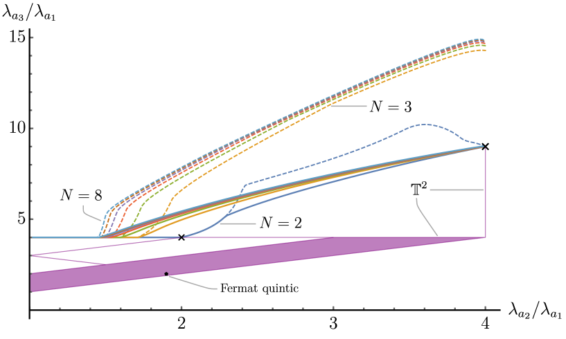
Refer to caption
Figure 15: Upper bounds on λa3/λa1subscript𝜆subscript𝑎3subscript𝜆subscript𝑎1\lambda_{a_{3}}/\lambda_{a_{1}} on closed Einstein manifolds with R0𝑅0R\geq 0 and N=2,,8𝑁28N=2,\dots,8, where λa{λa1,λa2}[λa3,)subscript𝜆𝑎subscript𝜆subscript𝑎1subscript𝜆subscript𝑎2subscript𝜆subscript𝑎3\lambda_{a}\in\{\lambda_{a_{1}},\lambda_{a_{2}}\}\cup[\lambda_{a_{3}},\infty) and we assume that λ0subscript𝜆0\lambda_{\mathcal{I}}\geq 0. The bounds represented by the solid lines take into account the symmetry of ga1a2a3subscript𝑔subscript𝑎1subscript𝑎2subscript𝑎3g_{a_{1}a_{2}a_{3}}, while the bounds represented by the dashed lines do not. The purple region, including the various purple lines, covers the image of the moduli space of flat 2-tori. The crosses mark the square 222-torus and very long flat N𝑁N-tori, while the pentagon marks the eigenvalues of the Fermat quintic threefold found numerically in Ref. [10].

Suppose now that the manifold has a 2subscript2\mathbb{Z}_{2} symmetry such that ψa1subscript𝜓subscript𝑎1\psi_{a_{1}} is odd and ψa2subscript𝜓subscript𝑎2\psi_{a_{2}} is even and let the nonzero scalar eigenvalues satisfy

λa{λa1}[λa3,),λa+[λa2,),formulae-sequencesuperscriptsubscript𝜆𝑎subscript𝜆subscript𝑎1subscript𝜆subscript𝑎3superscriptsubscript𝜆𝑎subscript𝜆subscript𝑎2\lambda_{a}^{-}\in\{\lambda_{a_{1}}\}\cup[\lambda_{a_{3}},\infty)\,,\quad\lambda_{a}^{+}\in[\lambda_{a_{2}},\infty)\,, (4.9)

where λa±superscriptsubscript𝜆𝑎plus-or-minus\lambda_{a}^{\pm} are the eigenvalues of the even/odd eigenfunctions. The consistency conditions (4) allow us to probe the ratio of the first two odd eigenvalues, λa3/λa1subscript𝜆subscript𝑎3subscript𝜆subscript𝑎1\lambda_{a_{3}}/\lambda_{a_{1}}. We again consider closed Einstein manifolds with R0𝑅0R\geq 0. To find bounds we solve the SDP obtained from the subset of the conditions in Eqs. (4.4) that are consistent with the 2subscript2\mathbb{Z}_{2} symmetry (imposing the symmetry of ga1a2a3subscript𝑔subscript𝑎1subscript𝑎2subscript𝑎3g_{a_{1}a_{2}a_{3}} does not help in this case). We obtain an upper bound on λa3/λa1subscript𝜆subscript𝑎3subscript𝜆subscript𝑎1\lambda_{a_{3}}/\lambda_{a_{1}} for each λa2/λa1(0,4]subscript𝜆subscript𝑎2subscript𝜆subscript𝑎104\lambda_{a_{2}}/\lambda_{a_{1}}\in(0,4] as shown in Figure 16, where we take λi0subscript𝜆𝑖0\lambda_{i}\geq 0 and either λ0subscript𝜆0\lambda_{\mathcal{I}}\geq 0 (solid lines) or λ/λa14subscript𝜆subscript𝜆subscript𝑎14\lambda_{\mathcal{I}}/\lambda_{a_{1}}\geq 4 (dashed lines). The very long flat N𝑁N-tori at position (4,9)49(4,9) saturate the λ0subscript𝜆0\lambda_{\mathcal{I}}\geq 0 bounds, as marked by the cross, and the round spheres lie at the edge of the λ/λa14subscript𝜆subscript𝜆subscript𝑎14\lambda_{\mathcal{I}}/\lambda_{a_{1}}\geq 4 bounds, as shown by the filled circles.
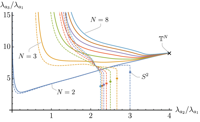
Refer to caption
Figure 16: Upper bounds on λa3/λa1subscript𝜆subscript𝑎3subscript𝜆subscript𝑎1\lambda_{a_{3}}/\lambda_{a_{1}} on closed Einstein manifolds with R0𝑅0R\geq 0 and a 2subscript2\mathbb{Z}_{2} symmetry for N=2,,8𝑁28N=2,\dots,8, where λa{λa1}[λa3,)superscriptsubscript𝜆𝑎subscript𝜆subscript𝑎1subscript𝜆subscript𝑎3\lambda_{a}^{-}\in\{\lambda_{a_{1}}\}\cup[\lambda_{a_{3}},\infty), λa+λa2superscriptsubscript𝜆𝑎subscript𝜆subscript𝑎2\lambda_{a}^{+}\geq\lambda_{a_{2}}, and either λ0subscript𝜆0\lambda_{\mathcal{I}}\geq 0 (solid lines) or λ/λa14subscript𝜆subscript𝜆subscript𝑎14\lambda_{\mathcal{I}}/\lambda_{a_{1}}\geq 4 (dashed lines). The filled circles correspond to the smallest distinct nonzero eigenvalues on SNsuperscript𝑆𝑁S^{N} and the cross corresponds to very long flat tori.

4.2 Bounds on vector couplings

Now we use the consistency conditions (4) to find bounds on the triple overlap integrals ga1a2isubscript𝑔subscript𝑎1subscript𝑎2𝑖g_{a_{1}a_{2}i}. These integrals were not accessible with the earlier consistency conditions since they are antisymmetric in a1subscript𝑎1a_{1} and a2subscript𝑎2a_{2}. Here we will focus on the case where the manifold has R0𝑅0R\geq 0 and the transverse eigenvector corresponds to a Killing vector, so that λi=2R/Nsubscript𝜆𝑖2𝑅𝑁\lambda_{i}=2R/N. This is possible when the manifold has a continuous symmetry. The quantity ga1a2isubscript𝑔subscript𝑎1subscript𝑎2𝑖g_{a_{1}a_{2}i} for iIKilling𝑖subscript𝐼Killingi\in I_{\rm Killing} can be non-vanishing only if λa1=λa2subscript𝜆subscript𝑎1subscript𝜆subscript𝑎2\lambda_{a_{1}}=\lambda_{a_{2}}. In the case of GR with a Ricci-flat internal manifold with a continuous symmetry, this quantity measures the Kaluza–Klein charge of the massive spin-2 states, q=2Vga1a2iMd(2d)/2𝑞2𝑉subscript𝑔subscript𝑎1subscript𝑎2𝑖superscriptsubscript𝑀𝑑2𝑑2q=\sqrt{2V}g_{a_{1}a_{2}i}M_{d}^{(2-d)/2}.

Following the same approach as in Section 3.2, we can use the consistency conditions to obtain upper bounds on the following scale invariant combination:

iIKillingga1a2i2Vλa1.subscript𝑖subscript𝐼Killingsuperscriptsubscript𝑔subscript𝑎1subscript𝑎2𝑖2𝑉subscript𝜆subscript𝑎1\sum_{i\in I_{\rm Killing}}g_{a_{1}a_{2}i}^{2}\frac{V}{\lambda_{a_{1}}}. (4.10)

In Figure 17 we plot the upper bounds on the square root of this quantity for closed Einstein manifolds with R>0𝑅0R>0 and N=2,,8𝑁28N=2,\dots,8, where we take λa1=λa2subscript𝜆subscript𝑎1subscript𝜆subscript𝑎2\lambda_{a_{1}}=\lambda_{a_{2}} as the smallest nonzero eigenvalue of the scalar Laplacian and we assume that λ0subscript𝜆0\lambda_{\mathcal{I}}\geq 0. We also mark points corresponding to certain modes on the round N𝑁N-spheres,999These have |ga1a2i|λa11/2V=(N+1)/2Nsubscript𝑔subscript𝑎1subscript𝑎2𝑖superscriptsubscript𝜆subscript𝑎112𝑉𝑁12𝑁|g_{a_{1}a_{2}i}|\lambda_{a_{1}}^{-1/2}\sqrt{V}=\sqrt{(N+1)/2N} and can be obtained from Yim(1,0,,0)proportional-tosubscriptsuperscript𝑌𝑚𝑖100Y^{m}_{i}\propto(1,0,\dots,0), corresponding to rotations in the θ1subscript𝜃1\theta_{1} direction, and ψa1=Y¯1,1,,1subscript𝜓subscript𝑎1subscript¯𝑌111\psi_{a_{1}}=\bar{Y}_{1,1,\dots,1}, ψa2=Y¯1,1,,1subscript𝜓subscript𝑎2subscript¯𝑌111\psi_{a_{2}}=\bar{Y}_{-1,1,\dots,1}, using the notation of Appendix A. which lie just below the upper bounds. For N>13𝑁13N>13, the bounds diverge above some finite value of λa1/Rsubscript𝜆subscript𝑎1𝑅\lambda_{a_{1}}/R. The dashed line gives the upper bound for Ricci-flat manifolds with N13𝑁13N\leq 13; this bound is saturated by flat tori, which is related to the saturation of the weak gravity conjecture by Kaluza–Klein modes in toroidal compactifications of gravity [38].
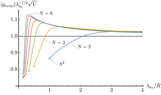
Refer to caption
Figure 17: Upper bounds on |ga1a2i|λa11/2Vsubscript𝑔subscript𝑎1subscript𝑎2𝑖superscriptsubscript𝜆subscript𝑎112𝑉|g_{a_{1}a_{2}i}|\lambda_{a_{1}}^{-1/2}\sqrt{V} for closed Einstein manifolds with R>0𝑅0R>0 and N=2,,8𝑁28N=2,\dots,8, where λi=2R/Nsubscript𝜆𝑖2𝑅𝑁\lambda_{i}=2R/N, λa1=λa2subscript𝜆subscript𝑎1subscript𝜆subscript𝑎2\lambda_{a_{1}}=\lambda_{a_{2}} is the smallest nonzero eigenvalue of the scalar Laplacian, and we have assumed that λ0subscript𝜆0\lambda_{\mathcal{I}}\geq 0. The markers correspond to the round spheres and the dashed line is the bound for Ricci-flat manifolds with N13𝑁13N\leq 13.

5 Discussion

We have developed a bootstrap approach to find bounds on the geometric data of closed Einstein manifolds. Specifically, our bounds constrain the eigenvalues and triple overlap integrals of eigenfunctions of various Laplacians. These bounds are found by starting with associativity conditions that must be satisfied by various higher-point integrals of eigenfunctions, then formulating them as semidefinite programming problems which can be solved numerically or analytically on a computer. This approach mirrors the conformal bootstrap. As far as we know, the bounds we find are new results about Einstein manifolds that have not appeared in the mathematical literature. Physically, these bounds can be thought of as constraints on the possible masses and three-point couplings of massive Kaluza–Klein modes in dimensional reductions of gravity.

There are several interesting directions that could be explored in the future. We have presented examples that illustrate some of the different types of bounds that can be deduced from the consistency conditions, but there should be many other examples that are worth exploring. It would also be worthwhile to try to find more powerful versions of the constraints studied here by looking for additional consistency conditions coming from higher-derivative integrands. Having a systematic or recursive method for finding these would be useful. This may not be possible without further assumptions, such as restricting to quotients of maximally symmetric manifolds (which still includes nontrivial spaces such as compact hyperbolic manifolds). On a technical level, the obstruction is due to the inevitable appearance of Riemann tensors in higher-derivative integrands. More conceptually, this is connected to the restrictions imposed by the consistent propagation of higher-spin particles in nontrivial gravitational backgrounds [39]. Perhaps string theory backgrounds satisfy additional consistency conditions that give more powerful bootstrap constraints.

Our results take the form of general bounds that apply to many Einstein manifolds. It would be interesting to see if consistency conditions are powerful enough to isolate rigid manifolds in “bootstrap islands” with only a small number of assumptions about the eigenvalues above the lightest modes, like what happens in the CFT bootstrap for strongly coupled CFTs such as the 3D Ising model at criticality [30, 36], and whether bootstrapping can be an efficient method to calculate the geometric data of manifolds of interest. This seems likely to require additional consistency conditions beyond those studied here. Other interesting directions would be to look for consistency conditions involving higher p𝑝p-forms or fermions, as would occur in dimensional reductions of supergravity; to search for consistency conditions for spaces other than closed manifolds, such as bounded domains in Euclidean space; and to incorporate symmetry constraints from more complicated isometry subgroups.

Acknowledgements:

We would like to thank Cliff Cheung for early discussions about the idea of this paper. We also thank Anthony Ashmore, Latham Boyle, and Sergei Dubovsky for helpful discussions and Mohamed Boucetta, Uwe Semmelmann, and Gregor Weingart for helpful correspondence. The authors acknowledge support from DOE grant DE-SC0019143 and Simons Foundation Award Number 658908.

Appendix A Compact rank one symmetric spaces

Here we briefly review some useful results about the geometric data of a few simple Einstein manifolds. We consider round spheres and the projective spaces over the reals \mathbb{R}, the complex numbers \mathbb{C}, the quaternions \mathbb{H}, and the octonians 𝕆𝕆\mathbb{O}, each with their standard metrics. These are the compact symmetric spaces of rank one.

A.1 Eigenvalues and eigenfunctions

Round spheres

Consider the N𝑁N-dimensional round sphere with unit radius, SNsuperscript𝑆𝑁S^{N}. This is the set of points that are unit distance from the origin in N+1superscript𝑁1\mathbb{R}^{N+1} with the metric induced from the standard Euclidean metric. It can also be described as the symmetric space SO(N+1)/SO(N)𝑆𝑂𝑁1𝑆𝑂𝑁SO(N+1)/SO(N). For (x1,,xN+1)N+1subscript𝑥1subscript𝑥𝑁1superscript𝑁1(x_{1},\dots,x_{N+1})\in\mathbb{R}^{N+1}, we can parameterize the sphere with spherical coordinates

x1=k=1Nsinθk,xα=cosθα1k=αNsinθk,α=2,,N+1,formulae-sequencesubscript𝑥1superscriptsubscriptproduct𝑘1𝑁subscript𝜃𝑘formulae-sequencesubscript𝑥𝛼subscript𝜃𝛼1superscriptsubscriptproduct𝑘𝛼𝑁subscript𝜃𝑘𝛼2𝑁1x_{1}=\prod_{k=1}^{N}\sin\theta_{k},\quad x_{\alpha}=\cos\theta_{\alpha-1}\prod_{k=\alpha}^{N}\sin\theta_{k},\quad\alpha=2,\dots,N+1, (A.1)

where 0θ1<2π0subscript𝜃12𝜋0\leq\theta_{1}<2\pi and 0θkπ0subscript𝜃𝑘𝜋0\leq\theta_{k}\leq\pi for 2kN2𝑘𝑁2\leq k\leq N. The metric in these coordinates is

dsS12=dθ12,dsSN2=sin2θNdsSN12+dθN2,N2.formulae-sequence𝑑subscriptsuperscript𝑠2superscript𝑆1𝑑superscriptsubscript𝜃12formulae-sequence𝑑subscriptsuperscript𝑠2superscript𝑆𝑁superscript2subscript𝜃𝑁𝑑subscriptsuperscript𝑠2superscript𝑆𝑁1𝑑superscriptsubscript𝜃𝑁2𝑁2\displaystyle ds^{2}_{S^{1}}=d\theta_{1}^{2},\quad ds^{2}_{S^{N}}=\sin^{2}\theta_{N}\,ds^{2}_{S^{N-1}}+d\theta_{N}^{2},\quad N\geq 2. (A.2)

The Ricci scalar and volume are

R=N(N1),V=2πN+12Γ[(N+1)/2].formulae-sequence𝑅𝑁𝑁1𝑉2superscript𝜋𝑁12Γdelimited-[]𝑁12R=N(N-1),\quad V=\frac{2\pi^{\frac{N+1}{2}}}{\Gamma\left[(N+1)/2\right]}. (A.3)

The eigenfunctions of the scalar Laplacian on SNsuperscript𝑆𝑁S^{N}, i.e, the (higher-dimensional) spherical harmonics, are obtained from the harmonic homogeneous polynomials in N+1superscript𝑁1\mathbb{R}^{N+1} restricted to the sphere [40]. They can be written in spherical coordinates in terms of associated Legendre polynomials [41]

YM1,,MN=eiM1θ12πk=2N(2Mk+k1)(Mk+Mk1+k2)!2(MkMk1)!sin2k2θkPMk+k22(Mk1+k22)(cosθk),subscript𝑌subscript𝑀1subscript𝑀𝑁superscript𝑒𝑖subscript𝑀1subscript𝜃12𝜋superscriptsubscriptproduct𝑘2𝑁2subscript𝑀𝑘𝑘1subscript𝑀𝑘subscript𝑀𝑘1𝑘22subscript𝑀𝑘subscript𝑀𝑘1superscript2𝑘2subscript𝜃𝑘superscriptsubscript𝑃subscript𝑀𝑘𝑘22subscript𝑀𝑘1𝑘22subscript𝜃𝑘Y_{M_{1},\dots,M_{N}}=\frac{e^{iM_{1}\theta_{1}}}{\sqrt{2\pi}}\prod_{k=2}^{N}\sqrt{\frac{(2M_{k}+k-1)(M_{k}+M_{k-1}+k-2)!}{2(M_{k}-M_{k-1})!}}\sin^{\frac{2-k}{2}}\theta_{k}P_{M_{k}+\frac{k-2}{2}}^{-(M_{k-1}+\frac{k-2}{2})}\left(\cos\theta_{k}\right), (A.4)

where Mksubscript𝑀𝑘M_{k} for k=1,,N𝑘1𝑁k=1,\dots,N are integers satisfying

|M1|M2MN1MNL.subscript𝑀1subscript𝑀2subscript𝑀𝑁1subscript𝑀𝑁𝐿|M_{1}|\leq M_{2}\leq\dots\leq M_{N-1}\leq M_{N}\equiv L. (A.5)

The spherical harmonics with a given value of L𝐿L transform into each other under rotations, forming the rank-L𝐿L symmetric traceless tensor representation of SO(N+1)𝑆𝑂𝑁1SO(N+1). Under parity they transform by an overall factor of (1)Lsuperscript1𝐿(-1)^{L}. In general they are complex, but we can define real spherical harmonics as (restricting to N>1𝑁1N>1)

Y¯M1,,MN1,L{(YM1,M2,,MN1,L+(1)M1YM1,M2,,MN1,L)/2ifM1>0,YM1,,MN1,LifM1=0,i(YM1,M2,,MN1,L(1)M1YM1,M2,,MN1,L)/2ifM1<0.subscript¯𝑌subscript𝑀1subscript𝑀𝑁1𝐿casessubscript𝑌subscript𝑀1subscript𝑀2subscript𝑀𝑁1𝐿superscript1subscript𝑀1subscript𝑌subscript𝑀1subscript𝑀2subscript𝑀𝑁1𝐿2ifsubscript𝑀10subscript𝑌subscript𝑀1subscript𝑀𝑁1𝐿ifsubscript𝑀10𝑖subscript𝑌subscript𝑀1subscript𝑀2subscript𝑀𝑁1𝐿superscript1subscript𝑀1subscript𝑌subscript𝑀1subscript𝑀2subscript𝑀𝑁1𝐿2ifsubscript𝑀10\overline{Y}_{M_{1},\dots,M_{N-1},L}\equiv\begin{cases}\left(Y_{-M_{1},M_{2},\dots,M_{N-1},L}+(-1)^{M_{1}}Y_{M_{1},M_{2},\dots,M_{N-1},L}\right)/\sqrt{2}\quad&{\rm if}\quad M_{1}>0,\\ Y_{M_{1},\dots,M_{N-1},L}\quad&{\rm if}\quad M_{1}=0,\\ i\left(Y_{M_{1},M_{2},\dots,M_{N-1},L}-(-1)^{M_{1}}Y_{-M_{1},M_{2},\dots,M_{N-1},L}\right)/\sqrt{2}\quad&{\rm if}\quad M_{1}<0.\end{cases} (A.6)

The corresponding eigenvalues are

λ=L(L+N1).𝜆𝐿𝐿𝑁1\lambda=L(L+N-1). (A.7)

A special subset of the spherical harmonics are the zonal spherical harmonics. These are eigenfunctions that are invariant under the SO(N)𝑆𝑂𝑁SO(N) rotations leaving a given point fixed. They are an example of zonal spherical functions, which are defined for general homogeneous spaces and always form a closed subsector of the consistency conditions. Taking the fixed point as (0,,0,1)n+1001superscript𝑛1(0,\dots,0,1)\in\mathbb{R}^{n+1}, the zonal harmonics can be written in terms of x 2x12++xN2superscript𝑥2superscriptsubscript𝑥12superscriptsubscript𝑥𝑁2\vec{x}^{\,2}\equiv x_{1}^{2}+\dots+x_{N}^{2} and xN+1subscript𝑥𝑁1x_{N+1}. For example, the first few nontrivial zonal spherical harmonics on S3superscript𝑆3S^{3} with unit L2superscript𝐿2L^{2}-norm are

L=1::𝐿1absent\displaystyle L=1: 2x4π=2cosθ3π,2subscript𝑥4𝜋2subscript𝜃3𝜋\displaystyle\quad\frac{\sqrt{2}x_{4}}{\pi}=\frac{\sqrt{2}\cos\theta_{3}}{\pi}, (A.8)
L=2::𝐿2absent\displaystyle L=2: 3x42x 22π=(1+2cos2θ3)2π,3superscriptsubscript𝑥42superscript𝑥22𝜋122subscript𝜃32𝜋\displaystyle\quad\frac{3x_{4}^{2}-\vec{x}^{\,2}}{\sqrt{2}\pi}=\frac{\left(1+2\cos 2\theta_{3}\right)}{\sqrt{2}\pi}, (A.9)
L=3::𝐿3absent\displaystyle L=3: 22x4(x42x 2)π=2(cosθ3+cos3θ3)π.22subscript𝑥4superscriptsubscript𝑥42superscript𝑥2𝜋2subscript𝜃33subscript𝜃3𝜋\displaystyle\quad\frac{2\sqrt{2}x_{4}\left(x_{4}^{2}-\vec{x}^{\,2}\right)}{\pi}=\frac{\sqrt{2}\left(\cos\theta_{3}+\cos 3\theta_{3}\right)}{\pi}. (A.10)

In general, the normalized zonal spherical harmonics are the spherical harmonics with Mk=0subscript𝑀𝑘0M_{k}=0 for k=1,,N1𝑘1𝑁1k=1,\dots,N-1 and can be written in terms of Gegenbauer polynomials,

Y0,,0,L=(2L+N1)Γ[N1]Γ[(N1)/2]Γ[L+1]4π(N+1)/2Γ[L+N1]CLN12(cosθN).subscript𝑌00𝐿2𝐿𝑁1Γdelimited-[]𝑁1Γdelimited-[]𝑁12Γdelimited-[]𝐿14superscript𝜋𝑁12Γdelimited-[]𝐿𝑁1superscriptsubscript𝐶𝐿𝑁12subscript𝜃𝑁Y_{0,\dots,0,L}=\sqrt{\frac{(2L+N-1)\Gamma[N-1]\Gamma\left[(N-1)/2\right]\Gamma[L+1]}{4\pi^{(N+1)/2}\Gamma[L+N-1]}}C_{L}^{\frac{N-1}{2}}\left(\cos\theta_{N}\right). (A.11)

Vector and tensor eigenmodes on SNsuperscript𝑆𝑁S^{N} can be obtained from contractions of certain mixed-symmetry constant tensors with the coordinates of N+1superscript𝑁1\mathbb{R}^{N+1} [42]. The eigenvalues of the Hodge Laplacian on transverse vectors are

λ=L(L+N1)+N2,L1,formulae-sequence𝜆𝐿𝐿𝑁1𝑁2𝐿subscriptabsent1\lambda=L(L+N-1)+N-2,\quad L\in\mathbb{Z}_{\geq 1}, (A.12)

and the eigenvalues of the Lichnerowicz Laplacian on symmetric transverse traceless 2-tensors are

λ=L(L+N1)+2(N1),L2,N>2.formulae-sequence𝜆𝐿𝐿𝑁12𝑁1formulae-sequence𝐿subscriptabsent2𝑁2\lambda=L(L+N-1)+2(N-1),\quad L\in\mathbb{Z}_{\geq 2},\quad N>2. (A.13)

Real projective space

The N𝑁N-dimensional real projective space Nsuperscript𝑁\mathbb{RP}^{N} is SN/2superscript𝑆𝑁subscript2S^{N}/\mathbb{Z}_{2}, where 2subscript2\mathbb{Z}_{2} acts as the antipodal map on SNsuperscript𝑆𝑁S^{N}. The eigenmodes on Nsuperscript𝑁\mathbb{RP}^{N} are thus proportional to the parity-even eigenmodes on SNsuperscript𝑆𝑁S^{N}, i.e., the scalar spherical harmonics and transverse traceless eigentensors with even L𝐿L and the transverse eigenvectors with odd L𝐿L.

Complex projective space

The complex projective space nsuperscript𝑛\mathbb{CP}^{n} with the Fubini–Study metric is the symmetric space U(n+1)/(U(n)×U(1))𝑈𝑛1𝑈𝑛𝑈1U(n+1)/(U(n)\times U(1)). Equivalently, it is the quotient space S2n+1/S1superscript𝑆2𝑛1superscript𝑆1S^{2n+1}/S^{1} obtained from the Hopf fibration. It has real dimension N=2n𝑁2𝑛N=2n. The Ricci scalar and volume are

R=4n(n+1),V=πnn!.formulae-sequence𝑅4𝑛𝑛1𝑉superscript𝜋𝑛𝑛R=4n(n+1),\quad V=\frac{\pi^{n}}{n!}. (A.14)

The complex projective line 1superscript1\mathbb{CP}^{1} is homothetic to S2superscript𝑆2S^{2}, i.e., isometric to a constant rescaling of S2superscript𝑆2S^{2}.

The eigenfunctions of the scalar Laplacian on nsuperscript𝑛\mathbb{CP}^{n} are obtained by projecting the spherical harmonics on S2n+1n+1superscript𝑆2𝑛1superscript𝑛1S^{2n+1}\subset\mathbb{C}^{n+1} that are invariant under U(1)=S1𝑈1superscript𝑆1U(1)=S^{1}, where the action of U(1)𝑈1U(1) on (z1,,zn+1)n+1subscript𝑧1subscript𝑧𝑛1superscript𝑛1(z_{1},\dots,z_{n+1})\in\mathbb{C}^{n+1} is multiplication by a phase [40]. The U(1)𝑈1U(1) invariants are thus ziz¯jsubscript𝑧𝑖subscript¯𝑧𝑗z_{i}\bar{z}_{j}. From Eq. (A.7), we get that the eigenvalues of the scalar Laplacian on nsuperscript𝑛\mathbb{CP}^{n} are

λk=4k(k+n),k0.formulae-sequencesubscript𝜆𝑘4𝑘𝑘𝑛𝑘subscriptabsent0\lambda_{k}=4k(k+n),\quad k\in\mathbb{Z}_{\geq 0}. (A.15)

The zonal spherical functions fixing the point (0,,0,1)n+1001superscript𝑛1(0,\dots,0,1)\in\mathbb{C}^{n+1} are the eigenfunctions that are further invariant under the action of U(n)𝑈𝑛U(n) on (z1,,zn)subscript𝑧1subscript𝑧𝑛(z_{1},\dots,z_{n}), so they can be written in terms of |z|2z1z¯1++znz¯nsuperscript𝑧2subscript𝑧1subscript¯𝑧1subscript𝑧𝑛subscript¯𝑧𝑛|\vec{z}\,|^{2}\equiv z_{1}\bar{z}_{1}+\dots+z_{n}\bar{z}_{n} and |zn+1|2superscriptsubscript𝑧𝑛12|z_{n+1}|^{2}. For example, the first few nontrivial zonal spherical functions on the complex projective plane 2superscript2\mathbb{CP}^{2} with unit L2superscript𝐿2L^{2}-norm are

k=1::𝑘1absent\displaystyle k=1: 2π(|z|22|zn+1|2),2𝜋superscript𝑧22superscriptsubscript𝑧𝑛12\displaystyle\quad\frac{2}{\pi}\left(|\vec{z}\,|^{2}-2|z_{n+1}|^{2}\right), (A.16)
k=2::𝑘2absent\displaystyle k=2: 6π(|z|46|z|2|zn+1|2+3|zn+1|4),6𝜋superscript𝑧46superscript𝑧2superscriptsubscript𝑧𝑛123superscriptsubscript𝑧𝑛14\displaystyle\quad\frac{\sqrt{6}}{\pi}\left(|\vec{z}\,|^{4}-6|\vec{z}\,|^{2}|z_{n+1}|^{2}+3|z_{n+1}|^{4}\right), (A.17)
k=3::𝑘3absent\displaystyle k=3: 22π(|z|612|z|4|zn+1|2+18|z|2|zn+1|44|zn+1|6).22𝜋superscript𝑧612superscript𝑧4superscriptsubscript𝑧𝑛1218superscript𝑧2superscriptsubscript𝑧𝑛144superscriptsubscript𝑧𝑛16\displaystyle\quad\frac{2\sqrt{2}}{\pi}\left(|\vec{z}\,|^{6}-12|\vec{z}\,|^{4}|z_{n+1}|^{2}+18|\vec{z}\,|^{2}|z_{n+1}|^{4}-4|z_{n+1}|^{6}\right). (A.18)

The smallest Lichnerowicz eigenvalue on transverse traceless symmetric 2-tensors on nsuperscript𝑛\mathbb{CP}^{n} with the Fubini-Study metric is λ1=32subscript𝜆subscript132\lambda_{\mathcal{I}_{1}}=32 for n=2𝑛2n=2 and λ1=8nsubscript𝜆subscript18𝑛\lambda_{\mathcal{I}_{1}}=8n for n3𝑛3n\geq 3 [33, 34].101010We thank Uwe Semmelmann and Gregor Weingart for sharing with us an extended version of Ref. [43], which helped us identify an error in the quoted value of λ1subscript𝜆subscript1\lambda_{\mathcal{I}_{1}} for nsuperscript𝑛\mathbb{CP}^{n} with n3𝑛3n\geq 3 in an earlier version of this paper.

Quaternionic projective space

The quaternionic projective space nsuperscript𝑛\mathbb{HP}^{n} with its standard metric is the quaternionic-Kähler symmetric space Sp(n+1)/(Sp(n)×Sp(1))Sp𝑛1Sp𝑛Sp1{\rm Sp}(n+1)/({\rm Sp}(n)\times{\rm Sp}(1)). Equivalently, it is the quotient space S4n+3/S3superscript𝑆4𝑛3superscript𝑆3S^{4n+3}/S^{3} obtained from the quaternionic Hopf fibration. It has real dimension N=4n𝑁4𝑛N=4n. The Ricci scalar and volume are

R=16n(n+2),V=π2n(2n+1)!.formulae-sequence𝑅16𝑛𝑛2𝑉superscript𝜋2𝑛2𝑛1R=16n(n+2)\,,\quad V=\frac{\pi^{2n}}{(2n+1)!}\,. (A.19)

The quaternionic projective line 1superscript1\mathbb{HP}^{1} is homothetic to S4superscript𝑆4S^{4}.

The eigenfunctions of the scalar Laplacian on nsuperscript𝑛\mathbb{HP}^{n} are obtained by projecting the spherical harmonics on S4n+3n+1superscript𝑆4𝑛3superscript𝑛1S^{4n+3}\subset\mathbb{H}^{n+1} that are invariant under Sp(1)=S3Sp1superscript𝑆3{\rm Sp}(1)=S^{3}, where the action of Sp(1)Sp1{\rm Sp}(1) on (q1,,qn+1)n+1subscript𝑞1subscript𝑞𝑛1superscript𝑛1(q_{1},\dots,q_{n+1})\in\mathbb{H}^{n+1} is right multiplication by unit quaternions. Writing a quaternion as a pair of complex numbers, qi=zi+wijsubscript𝑞𝑖subscript𝑧𝑖subscript𝑤𝑖𝑗q_{i}=z_{i}+w_{i}j, with quaternion conjugate q¯i=z¯iwijsubscript¯𝑞𝑖subscript¯𝑧𝑖subscript𝑤𝑖𝑗\bar{q}_{i}=\bar{z}_{i}-w_{i}j, the Sp(1)Sp1{\rm Sp}(1) invariants of interest are ziz¯j+wiw¯jsubscript𝑧𝑖subscript¯𝑧𝑗subscript𝑤𝑖subscript¯𝑤𝑗z_{i}\bar{z}_{j}+w_{i}\bar{w}_{j} [44]. From Eq. (A.7), we get that the eigenvalues of the scalar Laplacian on nsuperscript𝑛\mathbb{HP}^{n} are

λk=4k(k+2n+1),k0.formulae-sequencesubscript𝜆𝑘4𝑘𝑘2𝑛1𝑘subscriptabsent0\lambda_{k}=4k(k+2n+1),\quad k\in\mathbb{Z}_{\geq 0}. (A.20)

The zonal spherical functions on nsuperscript𝑛\mathbb{HP}^{n} fixing the point (0,,0,1)n+1001superscript𝑛1(0,\dots,0,1)\in\mathbb{H}^{n+1} are the eigenfunctions that are further invariant under the action of Sp(n)Sp𝑛{\rm Sp}(n) on (q1,,qn)subscript𝑞1subscript𝑞𝑛(q_{1},\dots,q_{n}), so they can be written in terms of |q|2q1q¯1++qnq¯nsuperscript𝑞2subscript𝑞1subscript¯𝑞1subscript𝑞𝑛subscript¯𝑞𝑛|\vec{q}\,|^{2}\equiv q_{1}\bar{q}_{1}+\dots+q_{n}\bar{q}_{n} and |qn+1|2qn+1q¯n+1superscriptsubscript𝑞𝑛12subscript𝑞𝑛1subscript¯𝑞𝑛1|q_{n+1}|^{2}\equiv q_{n+1}\bar{q}_{n+1}. For example, the first few nontrivial zonal spherical functions on the quaternionic projective plane 2superscript2\mathbb{HP}^{2} with unit L2superscript𝐿2L^{2}-norm are

k=1::𝑘1absent\displaystyle k=1: 2105π2(|q|22|qn+1|2),2105superscript𝜋2superscript𝑞22superscriptsubscript𝑞𝑛12\displaystyle\quad\frac{2\sqrt{105}}{\pi^{2}}\left(|\vec{q}\,|^{2}-2|q_{n+1}|^{2}\right), (A.21)
k=2::𝑘2absent\displaystyle k=2: 63π2(3|q|415|q|2|qn+1|2+10|qn+1|4),63superscript𝜋23superscript𝑞415superscript𝑞2superscriptsubscript𝑞𝑛1210superscriptsubscript𝑞𝑛14\displaystyle\quad\frac{6\sqrt{3}}{\pi^{2}}\left(3|\vec{q}\,|^{4}-15|\vec{q}\,|^{2}|q_{n+1}|^{2}+10|q_{n+1}|^{4}\right), (A.22)
k=3::𝑘3absent\displaystyle k=3: 2462π2(|q|69|q|4|qn+1|2+15|q|2|qn+1|45|qn+1|6).2462superscript𝜋2superscript𝑞69superscript𝑞4superscriptsubscript𝑞𝑛1215superscript𝑞2superscriptsubscript𝑞𝑛145superscriptsubscript𝑞𝑛16\displaystyle\quad\frac{2\sqrt{462}}{\pi^{2}}\left(|\vec{q}\,|^{6}-9|\vec{q}\,|^{4}|q_{n+1}|^{2}+15|\vec{q}\,|^{2}|q_{n+1}|^{4}-5|q_{n+1}|^{6}\right). (A.23)

Relatively little has been published about the Lichnerowicz eigenvalues of transverse traceless tensors on nsuperscript𝑛\mathbb{HP}^{n} for n>1𝑛1n>1. It is possible to get lower bounds on the first such eigenvalue using representation theory. From the results of Refs. [24, 45] we get λ16nsubscript𝜆16𝑛\lambda_{\mathcal{I}}\geq 16n.

Octonionic projective plane

The octonionic projective plane (or Cayley plane) 𝕆2𝕆superscript2\mathbb{OP}^{2} with its standard metric is the symmetric space F4/Spin(9)subscript𝐹4Spin9F_{4}/{\rm Spin}(9). It has real dimension N=16𝑁16N=16. In our normalization its Ricci scalar, volume, and scalar Laplacian eigenvalues are [40, 46]

R=144,V=3!(4π)811!,λk=k(k+11),k0,formulae-sequence𝑅144formulae-sequence𝑉3superscript4𝜋811formulae-sequencesubscript𝜆𝑘𝑘𝑘11𝑘subscriptabsent0R=144\,,\quad V=\frac{3!(4\pi)^{8}}{11!}\,,\quad\lambda_{k}=k(k+11),\quad k\in\mathbb{Z}_{\geq 0}\,, (A.24)

and from Refs. [45, 24] we get λ16subscript𝜆16\lambda_{\mathcal{I}}\geq 16. The octonionic projective line 𝕆1𝕆superscript1\mathbb{OP}^{1} is homothetic to S8superscript𝑆8S^{8} and 𝕆n𝕆superscript𝑛\mathbb{OP}^{n} does not exist for n>2𝑛2n>2 due to the non-associativity of the octonions.

A.2 Triple overlap integrals

The zonal spherical functions of the above manifolds can all be written in terms of Jacobi polynomials, Pk(α,β)(x)superscriptsubscript𝑃𝑘𝛼𝛽𝑥P_{k}^{(\alpha,\beta)}(x), which are a generalization of the Gegenbauer polynomials: the parameter k=0,1,2,𝑘012k=0,1,2,\dots labels the different eigenfunctions, the argument of the polynomial is x=cosd𝑥𝑑x=\cos d, where d𝑑d is the geodesic distance between a given point on the manifold and the fixed point, and the other parameters are given by α=(N2)/2𝛼𝑁22\alpha=(N-2)/2 and β=α,1/2,0,1𝛽𝛼1201\beta=\alpha,-1/2,0,1, or 333 for SNsuperscript𝑆𝑁S^{N}, Nsuperscript𝑁\mathbb{RP}^{N}, N/2superscript𝑁2\mathbb{CP}^{N/2}, N/4superscript𝑁4\mathbb{HP}^{N/4}, or 𝕆2𝕆superscript2\mathbb{OP}^{2}, respectively [47]. Labelling the zonal spherical functions by kisubscript𝑘𝑖k_{i}, this gives the following useful formula for their normalized triple overlap integrals, after substituting the appropriate values of α𝛼\alpha and β𝛽\beta:

Vgk1k2k3=n0α,βnk1α,βnk2α,βnk3α,β11𝑑x(1x)α(1+x)βPk1(α,β)(x)Pk2(α,β)(x)Pk3(α,β)(x),𝑉subscript𝑔subscript𝑘1subscript𝑘2subscript𝑘3superscriptsubscript𝑛0𝛼𝛽superscriptsubscript𝑛subscript𝑘1𝛼𝛽superscriptsubscript𝑛subscript𝑘2𝛼𝛽superscriptsubscript𝑛subscript𝑘3𝛼𝛽subscriptsuperscript11differential-d𝑥superscript1𝑥𝛼superscript1𝑥𝛽superscriptsubscript𝑃subscript𝑘1𝛼𝛽𝑥superscriptsubscript𝑃subscript𝑘2𝛼𝛽𝑥superscriptsubscript𝑃subscript𝑘3𝛼𝛽𝑥\sqrt{V}g_{k_{1}k_{2}k_{3}}=\frac{n_{0}^{\alpha,\beta}}{n_{k_{1}}^{\alpha,\beta}n_{k_{2}}^{\alpha,\beta}n_{k_{3}}^{\alpha,\beta}}\int^{1}_{-1}dx\,(1-x)^{\alpha}(1+x)^{\beta}P_{k_{1}}^{(\alpha,\beta)}(x)P_{k_{2}}^{(\alpha,\beta)}(x)P_{k_{3}}^{(\alpha,\beta)}(x)\,, (A.25)

where P0(α,β)(x)=1superscriptsubscript𝑃0𝛼𝛽𝑥1P_{0}^{(\alpha,\beta)}(x)=1 and the normalization constants are given by

(nkα,β)2superscriptsuperscriptsubscript𝑛𝑘𝛼𝛽2\displaystyle\left(n_{k}^{\alpha,\beta}\right)^{2} =11𝑑x(1x)α(1+x)β[Pk(α,β)(x)]2=2α+β+12k+α+β+1Γ[k+α+1]Γ[k+β+1]Γ[k+α+β+1]k!.absentsubscriptsuperscript11differential-d𝑥superscript1𝑥𝛼superscript1𝑥𝛽superscriptdelimited-[]superscriptsubscript𝑃𝑘𝛼𝛽𝑥2superscript2𝛼𝛽12𝑘𝛼𝛽1Γdelimited-[]𝑘𝛼1Γdelimited-[]𝑘𝛽1Γdelimited-[]𝑘𝛼𝛽1𝑘\displaystyle=\int^{1}_{-1}dx\,(1-x)^{\alpha}(1+x)^{\beta}\left[P_{k}^{(\alpha,\beta)}(x)\right]^{2}=\frac{2^{\alpha+\beta+1}}{2k+\alpha+\beta+1}\frac{\Gamma[k+\alpha+1]\Gamma[k+\beta+1]}{\Gamma[k+\alpha+\beta+1]k!}\,. (A.26)

Appendix B Deriving consistency conditions

In this appendix we show how to derive the eight consistency conditions involving two distinct fixed eigenfunctions, generalizing the discussion in Section 2.4.

From the identity111111Recall that the Wick contraction denotes that the indicated pair of fields is to be replaced by the appropriate eigenmode expansion from Section 2.3.

\contractionψa1ψa1\contractionψa1ψa1ψa2ψa2ψa1ψa1ψa2ψa2=\contractionψa1ψa1ψa2\contraction[2ex]ψa1ψa1ψa2ψa2ψa1ψa1ψa2ψa2,subscript\contractionsubscript𝜓subscript𝑎1subscript𝜓subscript𝑎1\contractionsubscript𝜓subscript𝑎1subscript𝜓subscript𝑎1subscript𝜓subscript𝑎2subscript𝜓subscript𝑎2subscript𝜓subscript𝑎1subscript𝜓subscript𝑎1subscript𝜓subscript𝑎2subscript𝜓subscript𝑎2subscript\contractionsubscript𝜓subscript𝑎1subscript𝜓subscript𝑎1subscript𝜓subscript𝑎2\contractiondelimited-[]2𝑒𝑥subscript𝜓subscript𝑎1subscript𝜓subscript𝑎1subscript𝜓subscript𝑎2subscript𝜓subscript𝑎2subscript𝜓subscript𝑎1subscript𝜓subscript𝑎1subscript𝜓subscript𝑎2subscript𝜓subscript𝑎2\int_{\mathcal{M}}\contraction{}{\psi_{a_{1}}}{}{\psi_{a_{1}}}\contraction{\psi_{a_{1}}\psi_{a_{1}}}{\psi_{a_{2}}}{}{\psi_{a_{2}}}\psi_{a_{1}}\psi_{a_{1}}\psi_{a_{2}}\psi_{a_{2}}=\int_{\mathcal{M}}\contraction{}{\psi_{a_{1}}}{\psi_{a_{1}}}{\psi_{a_{2}}}\contraction[2ex]{\psi_{a_{1}}}{\psi_{a_{1}}}{\psi_{a_{2}}}{\psi_{a_{2}}}\psi_{a_{1}}\psi_{a_{1}}\psi_{a_{2}}\psi_{a_{2}}, (B.1)

we get the consistency condition

a(ga1a1ga2a2aaga1a2a2)+V1(1δa1a2)=0.subscript𝑎subscript𝑔subscript𝑎1subscript𝑎1superscriptsubscript𝑔subscript𝑎2subscript𝑎2𝑎𝑎superscriptsubscript𝑔subscript𝑎1subscript𝑎2𝑎2superscript𝑉11subscript𝛿subscript𝑎1subscript𝑎20\sum_{a}\left(g_{a_{1}a_{1}}{}^{a}g_{a_{2}a_{2}a}-g_{a_{1}a_{2}a}^{2}\right)+V^{-1}\left(1-\delta_{a_{1}a_{2}}\right)=0. (B.2)

From the two identities involving two-derivative integrands,

\contractionψa1ψa2\contractionψa1ψa2mψa1mψa2ψa1ψa2mψa1mψa2=\contractionψa1ψa2mψa1\contraction[2ex]ψa1ψa2mψa1mψa2ψa1ψa2mψa1mψa2=\contraction[2ex]ψa1ψa2mψa1mψa2\contractionψa1ψa2mψa1ψa1ψa2mψa1mψa2,subscript\contractionsubscript𝜓subscript𝑎1subscript𝜓subscript𝑎2\contractionsubscript𝜓subscript𝑎1subscript𝜓subscript𝑎2subscript𝑚subscript𝜓subscript𝑎1superscript𝑚subscript𝜓subscript𝑎2subscript𝜓subscript𝑎1subscript𝜓subscript𝑎2subscript𝑚subscript𝜓subscript𝑎1superscript𝑚subscript𝜓subscript𝑎2subscript\contractionsubscript𝜓subscript𝑎1subscript𝜓subscript𝑎2subscript𝑚subscript𝜓subscript𝑎1\contractiondelimited-[]2𝑒𝑥subscript𝜓subscript𝑎1subscript𝜓subscript𝑎2subscript𝑚subscript𝜓subscript𝑎1superscript𝑚subscript𝜓subscript𝑎2subscript𝜓subscript𝑎1subscript𝜓subscript𝑎2subscript𝑚subscript𝜓subscript𝑎1superscript𝑚subscript𝜓subscript𝑎2subscript\contractiondelimited-[]2𝑒𝑥subscript𝜓subscript𝑎1subscript𝜓subscript𝑎2subscript𝑚subscript𝜓subscript𝑎1superscript𝑚subscript𝜓subscript𝑎2\contractionsubscript𝜓subscript𝑎1subscript𝜓subscript𝑎2subscript𝑚subscript𝜓subscript𝑎1subscript𝜓subscript𝑎1subscript𝜓subscript𝑎2subscript𝑚subscript𝜓subscript𝑎1superscript𝑚subscript𝜓subscript𝑎2\int_{\mathcal{M}}\contraction{}{\psi_{a_{1}}}{}{\psi_{a_{2}}}\contraction{\psi_{a_{1}}\psi_{a_{2}}}{\partial_{m}\psi_{a_{1}}}{}{\partial^{m}\psi_{a_{2}}}\psi_{a_{1}}\psi_{a_{2}}\partial_{m}\psi_{a_{1}}\partial^{m}\psi_{a_{2}}=\int_{\mathcal{M}}\contraction{}{\psi_{a_{1}}}{\psi_{a_{2}}}{\partial_{m}\psi_{a_{1}}}\contraction[2ex]{\psi_{a_{1}}}{\psi_{a_{2}}}{\partial_{m}\psi_{a_{1}}}{\partial^{m}\psi_{a_{2}}}\psi_{a_{1}}\psi_{a_{2}}\partial_{m}\psi_{a_{1}}\partial^{m}\psi_{a_{2}}=\int_{\mathcal{M}}\contraction[2ex]{}{\psi_{a_{1}}}{\psi_{a_{2}}\partial_{m}\psi_{a_{1}}}{\partial^{m}\psi_{a_{2}}}\contraction{\psi_{a_{1}}}{\psi_{a_{2}}}{}{\partial_{m}\psi_{a_{1}}}\psi_{a_{1}}\psi_{a_{2}}\partial_{m}\psi_{a_{1}}\partial^{m}\psi_{a_{2}}, (B.3)

we get the consistency conditions

a(2(λa1+λa2λa)ga1a2a2λaga1a1ga2a2aa)+4V1λa1δa1a2subscript𝑎2subscript𝜆subscript𝑎1subscript𝜆subscript𝑎2subscript𝜆𝑎superscriptsubscript𝑔subscript𝑎1subscript𝑎2𝑎2subscript𝜆𝑎subscript𝑔subscript𝑎1subscript𝑎1superscriptsubscript𝑔subscript𝑎2subscript𝑎2𝑎𝑎4superscript𝑉1subscript𝜆subscript𝑎1subscript𝛿subscript𝑎1subscript𝑎2\displaystyle\sum_{a}\left(2\left(\lambda_{a_{1}}+\lambda_{a_{2}}-\lambda_{a}\right)g_{a_{1}a_{2}a}^{2}-\lambda_{a}g_{a_{1}a_{1}}{}{}^{a}g_{a_{2}a_{2}a}\right)+4V^{-1}\lambda_{a_{1}}\delta_{a_{1}a_{2}} =0,absent0\displaystyle=0, (B.4)
4iga1a2i2+aλa1((λa1λa2)2+2λa(λa1+λa2)3λa2)ga1a2a2+4V1λa1δa1a24subscript𝑖superscriptsubscript𝑔subscript𝑎1subscript𝑎2𝑖2subscript𝑎superscriptsubscript𝜆𝑎1superscriptsubscript𝜆subscript𝑎1subscript𝜆subscript𝑎222subscript𝜆𝑎subscript𝜆subscript𝑎1subscript𝜆subscript𝑎23superscriptsubscript𝜆𝑎2superscriptsubscript𝑔subscript𝑎1subscript𝑎2𝑎24superscript𝑉1subscript𝜆subscript𝑎1subscript𝛿subscript𝑎1subscript𝑎2\displaystyle 4\sum_{i}g_{a_{1}a_{2}i}^{2}+\sum_{a}\lambda_{a}^{-1}\left((\lambda_{a_{1}}-\lambda_{a_{2}})^{2}+2\lambda_{a}(\lambda_{a_{1}}+\lambda_{a_{2}})-3\lambda_{a}^{2}\right)g_{a_{1}a_{2}a}^{2}+4V^{-1}\lambda_{a_{1}}\delta_{a_{1}a_{2}} =0.absent0\displaystyle=0. (B.5)

From the three identities involving four-derivative integrands,

\contraction(mψa1n)ψa2\contraction(mψa1n)ψa2(mψa1n)ψa2(mψa1n)ψa2(mψa1n)ψa2\displaystyle\int_{\mathcal{M}}\contraction{}{\partial_{(m}\psi_{a_{1}}}{}{\partial_{n)}\psi_{a_{2}}}\contraction{\partial_{(m}\psi_{a_{1}}\partial_{n)}\psi_{a_{2}}}{\partial^{(m}\psi_{a_{1}}}{}{\partial^{n)}\psi_{a_{2}}}\partial_{(m}\psi_{a_{1}}\partial_{n)}\psi_{a_{2}}\partial^{(m}\psi_{a_{1}}\partial^{n)}\psi_{a_{2}} =\contraction(mψa1n)ψa2(mψa1\contraction[2ex](mψa1n)ψa2(mψa1n)ψa2(mψa1n)ψa2(mψa1n)ψa2,\displaystyle=\int_{\mathcal{M}}\contraction{}{\partial_{(m}\psi_{a_{1}}}{\partial_{n)}\psi_{a_{2}}}{\partial^{(m}\psi_{a_{1}}}\contraction[2ex]{\partial_{(m}\psi_{a_{1}}}{\partial_{n)}\psi_{a_{2}}}{\partial^{(m}\psi_{a_{1}}}{\partial^{n)}\psi_{a_{2}}}\partial_{(m}\psi_{a_{1}}\partial_{n)}\psi_{a_{2}}\partial^{(m}\psi_{a_{1}}\partial^{n)}\psi_{a_{2}}, (B.6)
\contractionmψa1nψa1\contractionmψa1nψa1mψa2nψa2mψa1nψa1mψa2nψa2subscript\contractionsubscript𝑚subscript𝜓subscript𝑎1subscript𝑛subscript𝜓subscript𝑎1\contractionsubscript𝑚subscript𝜓subscript𝑎1subscript𝑛subscript𝜓subscript𝑎1superscript𝑚subscript𝜓subscript𝑎2superscript𝑛subscript𝜓subscript𝑎2subscript𝑚subscript𝜓subscript𝑎1subscript𝑛subscript𝜓subscript𝑎1superscript𝑚subscript𝜓subscript𝑎2superscript𝑛subscript𝜓subscript𝑎2\displaystyle\int_{\mathcal{M}}\contraction{}{\partial_{m}\psi_{a_{1}}}{}{\partial_{n}\psi_{a_{1}}}\contraction{\partial_{m}\psi_{a_{1}}\partial_{n}\psi_{a_{1}}}{\partial^{m}\psi_{a_{2}}}{}{\partial^{n}\psi_{a_{2}}}\partial_{m}\psi_{a_{1}}\partial_{n}\psi_{a_{1}}\partial^{m}\psi_{a_{2}}\partial^{n}\psi_{a_{2}} =\contractionmψa1nψa1mψa2\contraction[2ex]mψa1nψa1mψa2nψa2mψa1nψa1mψa2nψa2,absentsubscript\contractionsubscript𝑚subscript𝜓subscript𝑎1subscript𝑛subscript𝜓subscript𝑎1superscript𝑚subscript𝜓subscript𝑎2\contractiondelimited-[]2𝑒𝑥subscript𝑚subscript𝜓subscript𝑎1subscript𝑛subscript𝜓subscript𝑎1superscript𝑚subscript𝜓subscript𝑎2superscript𝑛subscript𝜓subscript𝑎2subscript𝑚subscript𝜓subscript𝑎1subscript𝑛subscript𝜓subscript𝑎1superscript𝑚subscript𝜓subscript𝑎2superscript𝑛subscript𝜓subscript𝑎2\displaystyle=\int_{\mathcal{M}}\contraction{}{\partial_{m}\psi_{a_{1}}}{\partial_{n}\psi_{a_{1}}}{\partial^{m}\psi_{a_{2}}}\contraction[2ex]{\partial_{m}\psi_{a_{1}}}{\partial_{n}\psi_{a_{1}}}{\partial^{m}\psi_{a_{2}}}{\partial^{n}\psi_{a_{2}}}\partial_{m}\psi_{a_{1}}\partial_{n}\psi_{a_{1}}\partial^{m}\psi_{a_{2}}\partial^{n}\psi_{a_{2}}, (B.7)
\contractionmψa1ψa2\contractionmψa1ψa2Δ(mψa1ψa2)mψa1ψa2Δ(mψa1ψa2)subscript\contractionsubscript𝑚subscript𝜓subscript𝑎1subscript𝜓subscript𝑎2\contractionsubscript𝑚subscript𝜓subscript𝑎1subscript𝜓subscript𝑎2Δsuperscript𝑚subscript𝜓subscript𝑎1subscript𝜓subscript𝑎2subscript𝑚subscript𝜓subscript𝑎1subscript𝜓subscript𝑎2Δsuperscript𝑚subscript𝜓subscript𝑎1subscript𝜓subscript𝑎2\displaystyle\int_{\mathcal{M}}\contraction{}{\partial_{m}\psi_{a_{1}}}{}{\psi_{a_{2}}}\contraction{\partial_{m}\psi_{a_{1}}\psi_{a_{2}}}{\Delta(\partial^{m}\psi_{a_{1}}}{}{\psi_{a_{2}})}\partial_{m}\psi_{a_{1}}\psi_{a_{2}}\Delta(\partial^{m}\psi_{a_{1}}\psi_{a_{2}}) =\contractionmψa1ψa2Δ(mψa1\contraction[2ex]mψa1ψa2Δ(mψa1ψa2)mψa1ψa2Δ(mψa1ψa2),\displaystyle=\int_{\mathcal{M}}\contraction{}{\partial_{m}\psi_{a_{1}}}{\psi_{a_{2}}}{\Delta(\partial^{m}\psi_{a_{1}}}\contraction[2ex]{\partial_{m}\psi_{a_{1}}}{\psi_{a_{2}}}{\Delta(\partial^{m}\psi_{a_{1}}}{\psi_{a_{2}})}\partial_{m}\psi_{a_{1}}\psi_{a_{2}}\Delta(\partial^{m}\psi_{a_{1}}\psi_{a_{2}}), (B.8)

we get the consistency conditions

8Nga1a22a[(N2)(λa1+λa2λa)2ga1a2a2+N(2λa1λa)(2λa2λa)ga1a1ga2a2aa]8𝑁subscriptsuperscriptsubscript𝑔subscript𝑎1subscript𝑎22subscript𝑎delimited-[]𝑁2superscriptsubscript𝜆subscript𝑎1subscript𝜆subscript𝑎2subscript𝜆𝑎2superscriptsubscript𝑔subscript𝑎1subscript𝑎2𝑎2𝑁2subscript𝜆subscript𝑎1subscript𝜆𝑎2subscript𝜆subscript𝑎2subscript𝜆𝑎subscript𝑔subscript𝑎1subscript𝑎1superscriptsubscript𝑔subscript𝑎2subscript𝑎2𝑎𝑎\displaystyle 8N\sum_{\mathcal{I}}g_{a_{1}a_{2}\mathcal{I}}^{2}-\sum_{a}\left[(N-2)\left(\lambda_{a_{1}}+\lambda_{a_{2}}-\lambda_{a}\right)^{2}g_{a_{1}a_{2}a}^{2}+N(2\lambda_{a_{1}}-\lambda_{a})(2\lambda_{a_{2}}-\lambda_{a})g_{a_{1}a_{1}}{}^{a}g_{a_{2}a_{2}a}\right]
+4N2iIKilling(λa1λa2)2ga1a2i2Nλi2R+aIconf.(N(λa1λa2)22λa(λa1+λa2)(N2)λa2)22λa((N1)λaR)ga1a2a24superscript𝑁2subscript𝑖subscript𝐼Killingsuperscriptsubscript𝜆subscript𝑎1subscript𝜆subscript𝑎22superscriptsubscript𝑔subscript𝑎1subscript𝑎2𝑖2𝑁subscript𝜆𝑖2𝑅subscript𝑎subscript𝐼confsuperscript𝑁superscriptsubscript𝜆subscript𝑎1subscript𝜆subscript𝑎222subscript𝜆𝑎subscript𝜆subscript𝑎1subscript𝜆subscript𝑎2𝑁2superscriptsubscript𝜆𝑎222subscript𝜆𝑎𝑁1subscript𝜆𝑎𝑅superscriptsubscript𝑔subscript𝑎1subscript𝑎2𝑎2\displaystyle+4N^{2}\sum_{i\notin I_{\rm Killing}}\frac{(\lambda_{a_{1}}-\lambda_{a_{2}})^{2}g_{a_{1}a_{2}i}^{2}}{N\lambda_{i}-2R}+\sum_{a\notin I_{\rm conf.}}\frac{\left(N(\lambda_{a_{1}}-\lambda_{a_{2}})^{2}-2\lambda_{a}(\lambda_{a_{1}}+\lambda_{a_{2}})-(N-2)\lambda_{a}^{2}\right)^{2}}{2\lambda_{a}\left((N-1)\lambda_{a}-R\right)}g_{a_{1}a_{2}a}^{2}
4V1λa1λa2((N2)δa1a2+N)=0,4superscript𝑉1subscript𝜆subscript𝑎1subscript𝜆subscript𝑎2𝑁2subscript𝛿subscript𝑎1subscript𝑎2𝑁0\displaystyle-4V^{-1}\lambda_{a_{1}}\lambda_{a_{2}}\left((N-2)\delta_{a_{1}a_{2}}+N\right)=0, (B.9)
4Nga1a1ga2a2+a[(2λa1λa)(2λa2λa)ga1a1ga2a2aaN(λa1+λa2λa)2ga1a2a2]4𝑁subscriptsubscript𝑔subscript𝑎1subscript𝑎1superscriptsubscript𝑔subscript𝑎2subscript𝑎2subscript𝑎delimited-[]2subscript𝜆subscript𝑎1subscript𝜆𝑎2subscript𝜆subscript𝑎2subscript𝜆𝑎subscript𝑔subscript𝑎1subscript𝑎1superscriptsubscript𝑔subscript𝑎2subscript𝑎2𝑎𝑎𝑁superscriptsubscript𝜆subscript𝑎1subscript𝜆subscript𝑎2subscript𝜆𝑎2superscriptsubscript𝑔subscript𝑎1subscript𝑎2𝑎2\displaystyle 4N\sum_{\mathcal{I}}g_{a_{1}a_{1}}{}^{\mathcal{I}}g_{a_{2}a_{2}\mathcal{I}}+\sum_{a}\left[\left(2\lambda_{a_{1}}-\lambda_{a}\right)\left(2\lambda_{a_{2}}-\lambda_{a}\right)g_{a_{1}a_{1}}{}{}^{a}g_{a_{2}a_{2}a}-N\left(\lambda_{a_{1}}+\lambda_{a_{2}}-\lambda_{a}\right)^{2}g_{a_{1}a_{2}a}^{2}\right]
+aIconf.λa(4λa1+(N2)λa)(4λa2+(N2)λa)ga1a1ga2a2aa4((N1)λaR)subscript𝑎subscript𝐼confsubscript𝜆𝑎4subscript𝜆subscript𝑎1𝑁2subscript𝜆𝑎4subscript𝜆subscript𝑎2𝑁2subscript𝜆𝑎subscript𝑔subscript𝑎1subscript𝑎1superscriptsubscript𝑔subscript𝑎2subscript𝑎2𝑎𝑎4𝑁1subscript𝜆𝑎𝑅\displaystyle+\sum_{a\notin I_{\rm conf.}}\frac{\lambda_{a}\left(4\lambda_{a_{1}}+(N-2)\lambda_{a}\right)\left(4\lambda_{a_{2}}+(N-2)\lambda_{a}\right)g_{a_{1}a_{1}}{}{}^{a}g_{a_{2}a_{2}a}}{4\left((N-1)\lambda_{a}-R\right)}
+4V1λa1λa2(1Nδa1a2)=0,4superscript𝑉1subscript𝜆subscript𝑎1subscript𝜆subscript𝑎21𝑁subscript𝛿subscript𝑎1subscript𝑎20\displaystyle+4V^{-1}\lambda_{a_{1}}\lambda_{a_{2}}(1-N\delta_{a_{1}a_{2}})=0, (B.10)
4iλiga1a2i2+a[(λa+λa1λa2)2ga1a2a2(2λa1λa)(2λa1+2λa2λa)ga1a1ga2a2aa]4subscript𝑖subscript𝜆𝑖superscriptsubscript𝑔subscript𝑎1subscript𝑎2𝑖2subscript𝑎delimited-[]superscriptsubscript𝜆𝑎subscript𝜆subscript𝑎1subscript𝜆subscript𝑎22superscriptsubscript𝑔subscript𝑎1subscript𝑎2𝑎22subscript𝜆subscript𝑎1subscript𝜆𝑎2subscript𝜆subscript𝑎12subscript𝜆subscript𝑎2subscript𝜆𝑎subscript𝑔subscript𝑎1subscript𝑎1superscriptsubscript𝑔subscript𝑎2subscript𝑎2𝑎𝑎\displaystyle 4\sum_{i}\lambda_{i}g_{a_{1}a_{2}i}^{2}+\sum_{a}\left[\left(\lambda_{a}+\lambda_{a_{1}}-\lambda_{a_{2}}\right)^{2}g_{a_{1}a_{2}a}^{2}-(2\lambda_{a_{1}}-\lambda_{a})(2\lambda_{a_{1}}+2\lambda_{a_{2}}-\lambda_{a})g_{a_{1}a_{1}}{}{}^{a}g_{a_{2}a_{2}a}\right]
4V1λa1(λa1+λa2)=0.4superscript𝑉1subscript𝜆subscript𝑎1subscript𝜆subscript𝑎1subscript𝜆subscript𝑎20\displaystyle-4V^{-1}\lambda_{a_{1}}(\lambda_{a_{1}}+\lambda_{a_{2}})=0. (B.11)

The remaining two consistency conditions are not straightforward to derive, even with guidance from the scattering amplitude results of Ref. [12]. They involve integrands that have six derivatives, which must be chosen carefully to cancel terms containing the Riemann tensor. One of them we get from

[\contractionmψa1nψa1\contractionmψa1nψa1ΔL(mψa2nψa2)mψa1nψa1ΔL(mψa2nψa2)+2\contraction(mψa1n)ψa2\contraction(mψa1n)ψa2ΔL((mψa1n)ψa2)(mψa1n)ψa2ΔL((mψa1n)ψa2)]\displaystyle\int_{\mathcal{M}}\left[\contraction{}{\partial_{m}\psi_{a_{1}}}{}{\partial_{n}\psi_{a_{1}}}\contraction{\partial_{m}\psi_{a_{1}}\partial_{n}\psi_{a_{1}}}{\Delta_{L}(\partial^{m}\psi_{a_{2}}}{}{\partial^{n}\psi_{a_{2}})}\partial_{m}\psi_{a_{1}}\partial_{n}\psi_{a_{1}}\Delta_{L}(\partial^{m}\psi_{a_{2}}\partial^{n}\psi_{a_{2}})+2\contraction{}{\partial_{(m}\psi_{a_{1}}}{}{\partial_{n)}\psi_{a_{2}}}\contraction{\partial_{(m}\psi_{a_{1}}\partial_{n)}\psi_{a_{2}}}{\Delta_{L}(\partial^{(m}\psi_{a_{1}}}{}{\partial^{n)}\psi_{a_{2}})}\partial_{(m}\psi_{a_{1}}\partial_{n)}\psi_{a_{2}}\Delta_{L}(\partial^{(m}\psi_{a_{1}}\partial^{n)}\psi_{a_{2}})\right]
=\displaystyle= [\contractionmψa1nψa1Δ(mψa2\contraction[2ex]mψa1nψa1ΔL(mψa2nψa2)mψa1nψa1ΔL(mψa2nψa2)+2\contraction(mψa1n)ψa2Δ((mψa1\contraction[2ex](mψa1n)ψa2ΔL((mψa1n)ψa2)(mψa1n)ψa2ΔL((mψa1n)ψa2)],\displaystyle\int_{\mathcal{M}}\left[\contraction{}{\partial_{m}\psi_{a_{1}}}{\partial_{n}\psi_{a_{1}}}{\Delta(\partial^{m}\psi_{a_{2}}}\contraction[2ex]{\partial_{m}\psi_{a_{1}}}{\partial_{n}\psi_{a_{1}}}{\Delta_{L}(\partial^{m}\psi_{a_{2}}}{\partial^{n}\psi_{a_{2}})}\partial_{m}\psi_{a_{1}}\partial_{n}\psi_{a_{1}}\Delta_{L}(\partial^{m}\psi_{a_{2}}\partial^{n}\psi_{a_{2}})+2\contraction{}{\partial_{(m}\psi_{a_{1}}}{\partial_{n)}\psi_{a_{2}}}{\Delta(\partial^{(m}\psi_{a_{1}}}\contraction[2ex]{\partial_{(m}\psi_{a_{1}}}{\partial_{n)}\psi_{a_{2}}}{\Delta_{L}(\partial^{(m}\psi_{a_{1}}}{\partial^{n)}\psi_{a_{2}})}\partial_{(m}\psi_{a_{1}}\partial_{n)}\psi_{a_{2}}\Delta_{L}(\partial^{(m}\psi_{a_{1}}\partial^{n)}\psi_{a_{2}})\right], (B.12)

where, after expanding the ΔLsubscriptΔ𝐿\Delta_{L}’s and adding a total derivative, the right-hand side can be written as

[\displaystyle\int_{\mathcal{M}}\Bigg{[} 2(λa1+λa2)\contractionmψa1mψa2\contractionmψa1mψa2nψa1nψa2mψa1mψa2nψa1nψa2+(λa1+λa2)\contractionmψa1mψa1\contractionmψa1mψa1nψa2nψa2mψa1mψa1nψa2nψa22subscript𝜆subscript𝑎1subscript𝜆subscript𝑎2\contractionsubscript𝑚subscript𝜓subscript𝑎1superscript𝑚subscript𝜓subscript𝑎2\contractionsubscript𝑚subscript𝜓subscript𝑎1superscript𝑚subscript𝜓subscript𝑎2subscript𝑛subscript𝜓subscript𝑎1superscript𝑛subscript𝜓subscript𝑎2subscript𝑚subscript𝜓subscript𝑎1superscript𝑚subscript𝜓subscript𝑎2subscript𝑛subscript𝜓subscript𝑎1superscript𝑛subscript𝜓subscript𝑎2subscript𝜆subscript𝑎1subscript𝜆subscript𝑎2\contractionsubscript𝑚subscript𝜓subscript𝑎1superscript𝑚subscript𝜓subscript𝑎1\contractionsubscript𝑚subscript𝜓subscript𝑎1superscript𝑚subscript𝜓subscript𝑎1subscript𝑛subscript𝜓subscript𝑎2superscript𝑛subscript𝜓subscript𝑎2subscript𝑚subscript𝜓subscript𝑎1superscript𝑚subscript𝜓subscript𝑎1subscript𝑛subscript𝜓subscript𝑎2superscript𝑛subscript𝜓subscript𝑎2\displaystyle 2(\lambda_{a_{1}}+\lambda_{a_{2}})\contraction{}{\partial_{m}\psi_{a_{1}}}{}{\partial^{m}\psi_{a_{2}}}\contraction{\partial_{m}\psi_{a_{1}}\partial^{m}\psi_{a_{2}}}{\partial_{n}\psi_{a_{1}}}{}{\partial^{n}\psi_{a_{2}}}\partial_{m}\psi_{a_{1}}\partial^{m}\psi_{a_{2}}\partial_{n}\psi_{a_{1}}\partial^{n}\psi_{a_{2}}+(\lambda_{a_{1}}+\lambda_{a_{2}})\contraction{}{\partial_{m}\psi_{a_{1}}}{}{\partial^{m}\psi_{a_{1}}}\contraction{\partial_{m}\psi_{a_{1}}\partial^{m}\psi_{a_{1}}}{\partial_{n}\psi_{a_{2}}}{}{\partial^{n}\psi_{a_{2}}}\partial_{m}\psi_{a_{1}}\partial^{m}\psi_{a_{1}}\partial_{n}\psi_{a_{2}}\partial^{n}\psi_{a_{2}}
2\contractionmψa1pmψa1\contractionmψa1pmψa1nψa2pnψa2mψa1pmψa1nψa2pnψa2\contractionp(mψa1mψa2)\contractionp(mψa1mψa2)p(nψa1nψa2)p(mψa1mψa2)p(nψa1nψa2)].\displaystyle-2\contraction{}{\partial_{m}\psi_{a_{1}}}{}{\nabla_{p}\partial^{m}\psi_{a_{1}}}\contraction{\partial_{m}\psi_{a_{1}}\nabla_{p}\partial^{m}\psi_{a_{1}}}{\partial_{n}\psi_{a_{2}}}{}{\nabla^{p}\partial^{n}\psi_{a_{2}}}\partial_{m}\psi_{a_{1}}\nabla_{p}\partial^{m}\psi_{a_{1}}\partial_{n}\psi_{a_{2}}\nabla^{p}\partial^{n}\psi_{a_{2}}-\contraction{}{\nabla_{p}(\partial_{m}\psi_{a_{1}}}{}{\partial^{m}\psi_{a_{2}})}\contraction{\nabla_{p}(\partial_{m}\psi_{a_{1}}\partial^{m}\psi_{a_{2}})}{\nabla^{p}(\partial_{n}\psi_{a_{1}}}{}{\partial^{n}\psi_{a_{2}})}\nabla_{p}(\partial_{m}\psi_{a_{1}}\partial^{m}\psi_{a_{2}})\nabla^{p}(\partial_{n}\psi_{a_{1}}\partial^{n}\psi_{a_{2}})\Bigg{]}. (B.13)

The remaining sum rule comes from

[\contractionmψa1nψa1\contractionmψa1nψa1ΔL(mψa2nψa2)mψa1nψa1ΔL(mψa2nψa2)\contractionΔ(mψa1ψa2)\contractionΔ(mψa1ψa2)Δ(mψa1ψa2)Δ(mψa1ψa2)Δ(mψa1ψa2)]subscriptdelimited-[]\contractionsubscript𝑚subscript𝜓subscript𝑎1subscript𝑛subscript𝜓subscript𝑎1\contractionsubscript𝑚subscript𝜓subscript𝑎1subscript𝑛subscript𝜓subscript𝑎1subscriptΔ𝐿superscript𝑚subscript𝜓subscript𝑎2superscript𝑛subscript𝜓subscript𝑎2subscript𝑚subscript𝜓subscript𝑎1subscript𝑛subscript𝜓subscript𝑎1subscriptΔ𝐿superscript𝑚subscript𝜓subscript𝑎2superscript𝑛subscript𝜓subscript𝑎2\contractionΔsubscript𝑚subscript𝜓subscript𝑎1subscript𝜓subscript𝑎2\contractionΔsubscript𝑚subscript𝜓subscript𝑎1subscript𝜓subscript𝑎2Δsuperscript𝑚subscript𝜓subscript𝑎1subscript𝜓subscript𝑎2Δsubscript𝑚subscript𝜓subscript𝑎1subscript𝜓subscript𝑎2Δsuperscript𝑚subscript𝜓subscript𝑎1subscript𝜓subscript𝑎2\displaystyle\int_{\mathcal{M}}\left[\contraction{}{\partial_{m}\psi_{a_{1}}}{}{\partial_{n}\psi_{a_{1}}}\contraction{\partial_{m}\psi_{a_{1}}\partial_{n}\psi_{a_{1}}}{\Delta_{L}(\partial^{m}\psi_{a_{2}}}{}{\partial^{n}\psi_{a_{2}})}\partial_{m}\psi_{a_{1}}\partial_{n}\psi_{a_{1}}\Delta_{L}(\partial^{m}\psi_{a_{2}}\partial^{n}\psi_{a_{2}})-\contraction{}{\Delta(\partial_{m}\psi_{a_{1}}}{}{\psi_{a_{2}})}\contraction{\Delta(\partial_{m}\psi_{a_{1}}\psi_{a_{2}})}{\Delta(\partial^{m}\psi_{a_{1}}}{}{\psi_{a_{2}})}\Delta(\partial_{m}\psi_{a_{1}}\psi_{a_{2}})\Delta(\partial^{m}\psi_{a_{1}}\psi_{a_{2}})\right]
=\displaystyle= [\contractionmψa1nψa1ΔL(mψa2\contraction[2ex]mψa1nψa1ΔL(mψa2nψa2)mψa1nψa1ΔL(mψa2nψa2)\contractionΔ(mψa1ψa2)Δ(mψa1\contraction[2ex]Δ(mψa1ψa2)Δ(mψa1ψa2)Δ(mψa1ψa2)Δ(mψa1ψa2)],\displaystyle\int_{\mathcal{M}}\left[\contraction{}{\partial_{m}\psi_{a_{1}}}{\partial_{n}\psi_{a_{1}}}{\Delta_{L}(\partial^{m}\psi_{a_{2}}}\contraction[2ex]{\partial_{m}\psi_{a_{1}}}{\partial_{n}\psi_{a_{1}}}{\Delta_{L}(\partial^{m}\psi_{a_{2}}}{\partial^{n}\psi_{a_{2}})}\partial_{m}\psi_{a_{1}}\partial_{n}\psi_{a_{1}}\Delta_{L}(\partial^{m}\psi_{a_{2}}\partial^{n}\psi_{a_{2}})-\contraction{}{\Delta(\partial_{m}\psi_{a_{1}}}{\psi_{a_{2}})}{\Delta(\partial^{m}\psi_{a_{1}}}\contraction[2ex]{\Delta(\partial_{m}\psi_{a_{1}}}{\psi_{a_{2}})}{\Delta(\partial^{m}\psi_{a_{1}}}{\psi_{a_{2}})}\Delta(\partial_{m}\psi_{a_{1}}\psi_{a_{2}})\Delta(\partial^{m}\psi_{a_{1}}\psi_{a_{2}})\right], (B.14)

where, after expanding the Laplacians and adding a total derivative, the right-hand side can be written as

[\displaystyle\int_{\mathcal{M}}\Bigg{[} \contractionmnψa1mnψa1\contractionmnψa1mnψa1pψa2pψa2mnψa1mnψa1pψa2pψa2+4\contractionmnψa1mnψa2\contractionmnψa1mnψa2pψa1pψa2mnψa1mnψa2pψa1pψa2+\contractionmnψa2mnψa2\contractionmnψa2mnψa2pψa1pψa1mnψa2mnψa2pψa1pψa1\contractionsubscript𝑚subscript𝑛subscript𝜓subscript𝑎1superscript𝑚superscript𝑛subscript𝜓subscript𝑎1\contractionsubscript𝑚subscript𝑛subscript𝜓subscript𝑎1superscript𝑚superscript𝑛subscript𝜓subscript𝑎1subscript𝑝subscript𝜓subscript𝑎2superscript𝑝subscript𝜓subscript𝑎2subscript𝑚subscript𝑛subscript𝜓subscript𝑎1superscript𝑚superscript𝑛subscript𝜓subscript𝑎1subscript𝑝subscript𝜓subscript𝑎2superscript𝑝subscript𝜓subscript𝑎24\contractionsubscript𝑚subscript𝑛subscript𝜓subscript𝑎1superscript𝑚superscript𝑛subscript𝜓subscript𝑎2\contractionsubscript𝑚subscript𝑛subscript𝜓subscript𝑎1superscript𝑚superscript𝑛subscript𝜓subscript𝑎2subscript𝑝subscript𝜓subscript𝑎1superscript𝑝subscript𝜓subscript𝑎2subscript𝑚subscript𝑛subscript𝜓subscript𝑎1superscript𝑚superscript𝑛subscript𝜓subscript𝑎2subscript𝑝subscript𝜓subscript𝑎1superscript𝑝subscript𝜓subscript𝑎2\contractionsubscript𝑚subscript𝑛subscript𝜓subscript𝑎2superscript𝑚superscript𝑛subscript𝜓subscript𝑎2\contractionsubscript𝑚subscript𝑛subscript𝜓subscript𝑎2superscript𝑚superscript𝑛subscript𝜓subscript𝑎2subscript𝑝subscript𝜓subscript𝑎1superscript𝑝subscript𝜓subscript𝑎1subscript𝑚subscript𝑛subscript𝜓subscript𝑎2superscript𝑚superscript𝑛subscript𝜓subscript𝑎2subscript𝑝subscript𝜓subscript𝑎1superscript𝑝subscript𝜓subscript𝑎1\displaystyle\contraction{}{\nabla_{m}\partial_{n}\psi_{a_{1}}}{}{\nabla^{m}\partial^{n}\psi_{a_{1}}}\contraction{\nabla_{m}\partial_{n}\psi_{a_{1}}\nabla^{m}\partial^{n}\psi_{a_{1}}}{\partial_{p}\psi_{a_{2}}}{}{\partial^{p}\psi_{a_{2}}}\nabla_{m}\partial_{n}\psi_{a_{1}}\nabla^{m}\partial^{n}\psi_{a_{1}}\partial_{p}\psi_{a_{2}}\partial^{p}\psi_{a_{2}}+4\contraction{}{\nabla_{m}\partial_{n}\psi_{a_{1}}}{}{\nabla^{m}\partial^{n}\psi_{a_{2}}}\contraction{\nabla_{m}\partial_{n}\psi_{a_{1}}\nabla^{m}\partial^{n}\psi_{a_{2}}}{\partial_{p}\psi_{a_{1}}}{}{\partial^{p}\psi_{a_{2}}}\nabla_{m}\partial_{n}\psi_{a_{1}}\nabla^{m}\partial^{n}\psi_{a_{2}}\partial_{p}\psi_{a_{1}}\partial^{p}\psi_{a_{2}}+\contraction{}{\nabla_{m}\partial_{n}\psi_{a_{2}}}{}{\nabla^{m}\partial^{n}\psi_{a_{2}}}\contraction{\nabla_{m}\partial_{n}\psi_{a_{2}}\nabla^{m}\partial^{n}\psi_{a_{2}}}{\partial_{p}\psi_{a_{1}}}{}{\partial^{p}\psi_{a_{1}}}\nabla_{m}\partial_{n}\psi_{a_{2}}\nabla^{m}\partial^{n}\psi_{a_{2}}\partial_{p}\psi_{a_{1}}\partial^{p}\psi_{a_{1}}
+6\contractionmψa1pmψa1\contractionmψa1pmψa1nψa2pnψa2mψa1pmψa1nψa2pnψa2+4(RNλa1)\contractionmψa1mψa2\contractionmψa1mψa2nψa1nψa2mψa1mψa2nψa1nψa26\contractionsubscript𝑚subscript𝜓subscript𝑎1subscript𝑝superscript𝑚subscript𝜓subscript𝑎1\contractionsubscript𝑚subscript𝜓subscript𝑎1subscript𝑝superscript𝑚subscript𝜓subscript𝑎1subscript𝑛subscript𝜓subscript𝑎2superscript𝑝superscript𝑛subscript𝜓subscript𝑎2subscript𝑚subscript𝜓subscript𝑎1subscript𝑝superscript𝑚subscript𝜓subscript𝑎1subscript𝑛subscript𝜓subscript𝑎2superscript𝑝superscript𝑛subscript𝜓subscript𝑎24𝑅𝑁subscript𝜆subscript𝑎1\contractionsubscript𝑚subscript𝜓subscript𝑎1superscript𝑚subscript𝜓subscript𝑎2\contractionsubscript𝑚subscript𝜓subscript𝑎1superscript𝑚subscript𝜓subscript𝑎2subscript𝑛subscript𝜓subscript𝑎1superscript𝑛subscript𝜓subscript𝑎2subscript𝑚subscript𝜓subscript𝑎1superscript𝑚subscript𝜓subscript𝑎2subscript𝑛subscript𝜓subscript𝑎1superscript𝑛subscript𝜓subscript𝑎2\displaystyle+6\contraction{}{\partial_{m}\psi_{a_{1}}}{}{\nabla_{p}\partial^{m}\psi_{a_{1}}}\contraction{\partial_{m}\psi_{a_{1}}\nabla_{p}\partial^{m}\psi_{a_{1}}}{\partial_{n}\psi_{a_{2}}}{}{\nabla^{p}\partial^{n}\psi_{a_{2}}}\partial_{m}\psi_{a_{1}}\nabla_{p}\partial^{m}\psi_{a_{1}}\partial_{n}\psi_{a_{2}}\nabla^{p}\partial^{n}\psi_{a_{2}}+4\left(\frac{R}{N}-\lambda_{a_{1}}\right)\contraction{}{\partial_{m}\psi_{a_{1}}}{}{\partial^{m}\psi_{a_{2}}}\contraction{\partial_{m}\psi_{a_{1}}\partial^{m}\psi_{a_{2}}}{\partial_{n}\psi_{a_{1}}}{}{\partial^{n}\psi_{a_{2}}}\partial_{m}\psi_{a_{1}}\partial^{m}\psi_{a_{2}}\partial_{n}\psi_{a_{1}}\partial^{n}\psi_{a_{2}}
(λa12+2λa2λa1+2λa22)\contractionmψa1mψa1\contractionmψa1mψa1ψa2ψa2mψa1mψa1ψa2ψa2+2λa1λa2\contractionmψa1mψa2\contractionmψa1mψa2ψa1ψa2mψa1mψa2ψa1ψa2λa12\contractionmψa2mψa2\contractionmψa2mψa2ψa1ψa1mψa2mψa2ψa1ψa1superscriptsubscript𝜆subscript𝑎122subscript𝜆subscript𝑎2subscript𝜆subscript𝑎12superscriptsubscript𝜆subscript𝑎22\contractionsubscript𝑚subscript𝜓subscript𝑎1superscript𝑚subscript𝜓subscript𝑎1\contractionsubscript𝑚subscript𝜓subscript𝑎1superscript𝑚subscript𝜓subscript𝑎1subscript𝜓subscript𝑎2subscript𝜓subscript𝑎2subscript𝑚subscript𝜓subscript𝑎1superscript𝑚subscript𝜓subscript𝑎1subscript𝜓subscript𝑎2subscript𝜓subscript𝑎22subscript𝜆subscript𝑎1subscript𝜆subscript𝑎2\contractionsubscript𝑚subscript𝜓subscript𝑎1superscript𝑚subscript𝜓subscript𝑎2\contractionsubscript𝑚subscript𝜓subscript𝑎1superscript𝑚subscript𝜓subscript𝑎2subscript𝜓subscript𝑎1subscript𝜓subscript𝑎2subscript𝑚subscript𝜓subscript𝑎1superscript𝑚subscript𝜓subscript𝑎2subscript𝜓subscript𝑎1subscript𝜓subscript𝑎2superscriptsubscript𝜆subscript𝑎12\contractionsubscript𝑚subscript𝜓subscript𝑎2superscript𝑚subscript𝜓subscript𝑎2\contractionsubscript𝑚subscript𝜓subscript𝑎2superscript𝑚subscript𝜓subscript𝑎2subscript𝜓subscript𝑎1subscript𝜓subscript𝑎1subscript𝑚subscript𝜓subscript𝑎2superscript𝑚subscript𝜓subscript𝑎2subscript𝜓subscript𝑎1subscript𝜓subscript𝑎1\displaystyle-(\lambda_{a_{1}}^{2}+2\lambda_{a_{2}}\lambda_{a_{1}}+2\lambda_{a_{2}}^{2})\contraction{}{\partial_{m}\psi_{a_{1}}}{}{\partial^{m}\psi_{a_{1}}}\contraction{\partial_{m}\psi_{a_{1}}\partial^{m}\psi_{a_{1}}}{\psi_{a_{2}}}{}{\psi_{a_{2}}}\partial_{m}\psi_{a_{1}}\partial^{m}\psi_{a_{1}}\psi_{a_{2}}\psi_{a_{2}}+2\lambda_{a_{1}}\lambda_{a_{2}}\contraction{}{\partial_{m}\psi_{a_{1}}}{}{\partial^{m}\psi_{a_{2}}}\contraction{\partial_{m}\psi_{a_{1}}\partial^{m}\psi_{a_{2}}}{\psi_{a_{1}}}{}{\psi_{a_{2}}}\partial_{m}\psi_{a_{1}}\partial^{m}\psi_{a_{2}}\psi_{a_{1}}\psi_{a_{2}}-\lambda_{a_{1}}^{2}\contraction{}{\partial_{m}\psi_{a_{2}}}{}{\partial^{m}\psi_{a_{2}}}\contraction{\partial_{m}\psi_{a_{2}}\partial^{m}\psi_{a_{2}}}{\psi_{a_{1}}}{}{\psi_{a_{1}}}\partial_{m}\psi_{a_{2}}\partial^{m}\psi_{a_{2}}\psi_{a_{1}}\psi_{a_{1}}
+4(λa1+λa2)\contractionmψa1nmψa1\contractionmψa1nmψa1ψa2nψa2mψa1nmψa1ψa2nψa2+2RN\contractionmψa1mψa1\contractionmψa1mψa1nψa2nψa2mψa1mψa1nψa2nψa2].\displaystyle+4(\lambda_{a_{1}}+\lambda_{a_{2}})\contraction{}{\partial_{m}\psi_{a_{1}}}{}{\nabla_{n}\partial^{m}\psi_{a_{1}}}\contraction{\partial_{m}\psi_{a_{1}}\nabla_{n}\partial^{m}\psi_{a_{1}}}{\psi_{a_{2}}}{}{\partial^{n}\psi_{a_{2}}}\partial_{m}\psi_{a_{1}}\nabla_{n}\partial^{m}\psi_{a_{1}}\psi_{a_{2}}\partial^{n}\psi_{a_{2}}+\frac{2R}{N}\contraction{}{\partial_{m}\psi_{a_{1}}}{}{\partial^{m}\psi_{a_{1}}}\contraction{\partial_{m}\psi_{a_{1}}\partial^{m}\psi_{a_{1}}}{\partial_{n}\psi_{a_{2}}}{}{\partial^{n}\psi_{a_{2}}}\partial_{m}\psi_{a_{1}}\partial^{m}\psi_{a_{1}}\partial_{n}\psi_{a_{2}}\partial^{n}\psi_{a_{2}}\Bigg{]}. (B.15)

These two identities give the consistency conditions

4Niλi2ga1a2i2+8Nλga1a224NV1λa1((1+2δa1a2)λa12+3λa1λa2+2λa22)4𝑁subscript𝑖superscriptsubscript𝜆𝑖2superscriptsubscript𝑔subscript𝑎1subscript𝑎2𝑖28𝑁subscriptsubscript𝜆superscriptsubscript𝑔subscript𝑎1subscript𝑎224𝑁superscript𝑉1subscript𝜆subscript𝑎112subscript𝛿subscript𝑎1subscript𝑎2superscriptsubscript𝜆subscript𝑎123subscript𝜆subscript𝑎1subscript𝜆subscript𝑎22superscriptsubscript𝜆subscript𝑎22\displaystyle 4N\sum_{i}\lambda_{i}^{2}g_{a_{1}a_{2}i}^{2}+8N\sum_{\mathcal{I}}\lambda_{\mathcal{I}}g_{a_{1}a_{2}\mathcal{I}}^{2}-4NV^{-1}\lambda_{a_{1}}\left((1+2\delta_{a_{1}a_{2}})\lambda_{a_{1}}^{2}+3\lambda_{a_{1}}\lambda_{a_{2}}+2\lambda_{a_{2}}^{2}\right)
+a[N(4λa1(λa1+λa2)(λa1+2λa2)+4(λa1+λa2)(2λa1+λa2)λa4(λa1+λa2)λa2+λa3)ga1a1ga2a2aa\displaystyle+\sum_{a}\Big{[}N\left(-4\lambda_{a_{1}}(\lambda_{a_{1}}+\lambda_{a_{2}})(\lambda_{a_{1}}+2\lambda_{a_{2}})+4(\lambda_{a_{1}}+\lambda_{a_{2}})(2\lambda_{a_{1}}+\lambda_{a_{2}})\lambda_{a}-4(\lambda_{a_{1}}+\lambda_{a_{2}})\lambda_{a}^{2}+\lambda_{a}^{3}\right)g_{a_{1}a_{1}}{}^{a}g_{a_{2}a_{2}a}
+2(2Nλa12(λa1+λa2)+((1+4N)λa12+2λa1λa2+λa22)λa2(λa1+λa2)λa2+λa3)ga1a2a2]\displaystyle+2\left(-2N\lambda_{a_{1}}^{2}(\lambda_{a_{1}}+\lambda_{a_{2}})+((1+4N)\lambda_{a_{1}}^{2}+2\lambda_{a_{1}}\lambda_{a_{2}}+\lambda_{a_{2}}^{2})\lambda_{a}-2(\lambda_{a_{1}}+\lambda_{a_{2}})\lambda_{a}^{2}+\lambda_{a}^{3}\right)g_{a_{1}a_{2}a}^{2}\Big{]}
+4N2iIKillingλi(λa1λa2)2ga1a2i2Nλi2R+aIconf.(N(λa1λa2)22λa(λa1+λa2)(N2)λa2)2ga1a2a22((N1)λaR)=0,4superscript𝑁2subscript𝑖subscript𝐼Killingsubscript𝜆𝑖superscriptsubscript𝜆subscript𝑎1subscript𝜆subscript𝑎22superscriptsubscript𝑔subscript𝑎1subscript𝑎2𝑖2𝑁subscript𝜆𝑖2𝑅subscript𝑎subscript𝐼confsuperscript𝑁superscriptsubscript𝜆subscript𝑎1subscript𝜆subscript𝑎222subscript𝜆𝑎subscript𝜆subscript𝑎1subscript𝜆subscript𝑎2𝑁2superscriptsubscript𝜆𝑎22superscriptsubscript𝑔subscript𝑎1subscript𝑎2𝑎22𝑁1subscript𝜆𝑎𝑅0\displaystyle+4N^{2}\sum_{i\notin I_{\rm Killing}}\frac{\lambda_{i}(\lambda_{a_{1}}-\lambda_{a_{2}})^{2}g_{a_{1}a_{2}i}^{2}}{N\lambda_{i}-2R}+\sum_{a\notin I_{\rm conf.}}\frac{\left(N(\lambda_{a_{1}}-\lambda_{a_{2}})^{2}-2\lambda_{a}(\lambda_{a_{1}}+\lambda_{a_{2}})-(N-2)\lambda_{a}^{2}\right)^{2}g_{a_{1}a_{2}a}^{2}}{2((N-1)\lambda_{a}-R)}=0, (B.16)
16Nλga1a1ga2a216Niλi2ga1a2i2+16NV1λa1(λa122(δa1a21)λa1λa2+λa22)16𝑁subscriptsubscript𝜆subscript𝑔subscript𝑎1subscript𝑎1superscriptsubscript𝑔subscript𝑎2subscript𝑎216𝑁subscript𝑖superscriptsubscript𝜆𝑖2superscriptsubscript𝑔subscript𝑎1subscript𝑎2𝑖216𝑁superscript𝑉1subscript𝜆subscript𝑎1superscriptsubscript𝜆subscript𝑎122subscript𝛿subscript𝑎1subscript𝑎21subscript𝜆subscript𝑎1subscript𝜆subscript𝑎2superscriptsubscript𝜆subscript𝑎22\displaystyle 16N\sum_{\mathcal{I}}\lambda_{\mathcal{I}}g_{a_{1}a_{1}}{}^{\mathcal{I}}g_{a_{2}a_{2}\mathcal{I}}-16N\sum_{i}\lambda_{i}^{2}g_{a_{1}a_{2}i}^{2}+16NV^{-1}\lambda_{a_{1}}\left(\lambda_{a_{1}}^{2}-2(\delta_{a_{1}a_{2}}-1)\lambda_{a_{1}}\lambda_{a_{2}}+\lambda_{a_{2}}^{2}\right)
+a[4N(2(λa1+λa2)(λa122λa1λa2λa22)(3λa1210λa1λa25λa22)λa4(λa1+λa2)λa2+λa3)ga1a2a2\displaystyle+\sum_{a}\Big{[}4N\left(2(\lambda_{a_{1}}+\lambda_{a_{2}})(\lambda_{a_{1}}^{2}-2\lambda_{a_{1}}\lambda_{a_{2}}-\lambda^{2}_{a_{2}})-(3\lambda_{a_{1}}^{2}-10\lambda_{a_{1}}\lambda_{a_{2}}-5\lambda_{a_{2}}^{2})\lambda_{a}-4(\lambda_{a_{1}}+\lambda_{a_{2}})\lambda_{a}^{2}+\lambda_{a}^{3}\right)g_{a_{1}a_{2}a}^{2}
+(16Nλa1(λa1+λa2)28(3Nλa12+(3N2)λa1λa2+Nλa22)λa+8(N1)(λa1+λa2)λa22(N2)λa3)ga1a1ga2a2aa]\displaystyle+\left(16N\lambda_{a_{1}}(\lambda_{a_{1}}+\lambda_{a_{2}})^{2}-8(3N\lambda_{a_{1}}^{2}+(3N-2)\lambda_{a_{1}}\lambda_{a_{2}}+N\lambda_{a_{2}}^{2})\lambda_{a}+8(N-1)(\lambda_{a_{1}}+\lambda_{a_{2}})\lambda_{a}^{2}-2(N-2)\lambda_{a}^{3}\right)g_{a_{1}a_{1}}{}^{a}g_{a_{2}a_{2}a}\Big{]}
+aIconf.λa2(4λa1+(N2)λa)(4λa2+(N2)λa)ga1a1ga2a2aa(N1)λaR=0.subscript𝑎subscript𝐼confsuperscriptsubscript𝜆𝑎24subscript𝜆subscript𝑎1𝑁2subscript𝜆𝑎4subscript𝜆subscript𝑎2𝑁2subscript𝜆𝑎subscript𝑔subscript𝑎1subscript𝑎1superscriptsubscript𝑔subscript𝑎2subscript𝑎2𝑎𝑎𝑁1subscript𝜆𝑎𝑅0\displaystyle+\sum_{a\notin I_{\rm conf.}}\frac{\lambda_{a}^{2}\left(4\lambda_{a_{1}}+(N-2)\lambda_{a}\right)\left(4\lambda_{a_{2}}+(N-2)\lambda_{a}\right)g_{a_{1}a_{1}}{}^{a}g_{a_{2}a_{2}a}}{(N-1)\lambda_{a}-R}=0. (B.17)

These eight consistency conditions reduce to those given in Eq. (2.28) when a1=a2subscript𝑎1subscript𝑎2a_{1}=a_{2}.

References