What if ALP dark matter for the XENON1T excess is the inflaton

Abstract

The recent XENON1T excess in the electron recoil data can be explained by anomaly-free axion-like particle (ALP) dark matter with mass $m_{\phi}=2.3\pm 0.2$ keV and the decay constant $f_{\phi}/q_{e}\simeq 2\times 10^{10}\sqrt{\Omega_{\phi}/\Omega_{\rm DM}}{\rm\,GeV}$. Intriguingly, the suggested mass and decay constant are consistent with the relation, $f_{\phi}\sim 10^{3}\sqrt{m_{\phi}M_{p}}$, predicted in a scenario where the ALP plays the role of the inflaton. This raises a possibility that the ALP dark matter responsible for the XENON1T excess also drove inflation in the very early universe. We study implications of the XENON1T excess for the ALP inflation and thermal history of the universe after inflation.

1 Introduction

Recently, an excess was found in the electron recoil data collected by the XENON1T experiment [1], which stimulated active discussion on the possible explanation for the excess. While the tritium is not excluded as a mundane explanation, it is worth studying the interpretation in terms of new physics beyond the standard model (SM).

One of such is the axion-like particle (ALP) dark matter (DM) [3, 4, 5] (see Refs. [6, 7, 8, 9, 10, 11, 12] for reviews), which generates a mono-energetic peak through absorption by electron. The XENON1T excess favors the ALP mass and coupling to electron in the range of

$$m_{\phi} =2.3\pm 0.2{\rm\,keV}\,\,(68\%{\rm\,C.L.}),$$ (1.1)

$$g_{\phi e} \simeq 3\times 10^{-14}\sqrt{\frac{\Omega_{\rm DM}}{\Omega_{\phi}}},$$ (1.2)

with a $3.0\,\sigma$ global ($4.0\,\sigma$ local) significance over background [1], where $\Omega_{\rm DM}$ and $\Omega_{\phi}$ are the density parameters of DM and ALP $\phi$, respectively. Let us define the fraction of ALP DM by $r\equiv\Omega_{\phi}/\Omega_{\rm DM}$. One can express the coupling to electrons in terms of the decay constant as

$$f_{\phi} \simeq 2\times 10^{10}q_{e}\sqrt{r}{\rm\,GeV},$$ (1.3)

where $q_{e}$ is the Peccei-Quinn (PQ) charge of the electron. Since the ALP generically has an anomalous coupling to photons, its decay produces X-ray line signal at an energy equal to half the ALP mass. To satisfy the X-ray observations for the above mass and decay constant, however, the ALP coupling to photons must be extremely suppressed than naively expected [16, 8, 17, 3]. One way to suppress the photon coupling is to consider an anomaly-free ALP which has no QED anomaly [17, 3]. Then, the dominant coupling to photons arises from the electron threshold of the form,

$$\frac{\alpha}{48\pi(f_{\phi}/q_{e})}\frac{\partial^{2}\phi}{m_{e}^{2}}F_{\mu\nu}\tilde{F}^{\mu\nu},$$ (1.4)

which predicts an X-ray line signal with definite strength [17, 3] (see also Ref. [16]). The predicted X-ray line may be searched for by future X-ray observatories [18, 19, 20, 21].

The coupling to electron (1.2) satisfies the stellar cooling bound, and actually it is close to the value hinted by the stellar cooling anomalies of white dwarfs (WD) [22, 23] and red giants (RG) [24], and the agreement becomes even better if the ALP is a part of the total DM [3]. Furthermore, the right abundance of ALP DM can be generated by the misalignment mechanism, or by thermal scatterings if the ALP constitutes a fraction of DM [8, 17, 3]. In this paper we will point out another coincidence of the ALP parameters in a different context.

There is a strong evidence [26] for inflation at an early stage of the universe [27, 28, 29]. The slow-roll inflation paradigm [30, 31] crucially depends on a sufficiently flat inflaton potential, and it has been one of the central issues in the inflation model building how to protect the flat potential from radiative corrections since the early discussion on the GUT higgs inflation in the 1980s. One of the plausible candidates for the inflaton is an axion whose potential is naturally protected by the shift symmetry.

There are a wide variety of inflation models based on the axion. Natural inflation [32] is a simple and therefore attractive model in which the inflaton potential consists of a single cosine function. However, the decay constant is required to be super-Planckian for the slow-roll inflation, and its predicted scalar spectral index as well as the tensor-to-scalar ratio are disfavored by the current CMB observations [26]. There are many extensions of the natural inflation (see e.g. Refs. [33, 34, 35, 36, 37, 38, 39, 40]), and we focus on the simplest class of the so-called multi-natural inflation [34]; the inflaton potential consists of two cosine terms which conspire to make a flat plateau around the potential maximum. This potential allows slow-roll inflation from very high energy scales to very low energy scales depending on the value of the decay constant. Such axion inflation model may be realized in the axion landscape [41, 42] where many axions have various shift symmetry breaking terms and mixing.

In the simplest class of the multi-natural inflation, the inflaton potential often has an upside-down symmetry, where the curvatures of the potential maximum and minimum are of equal magnitude but opposite sign (see Fig. 1). Then, the inflaton mass at the minimum is naturally suppressed once we require the slow-roll conditions to be satisfied around the potential maximum. Thanks to the light mass, the inflaton can be stable on the cosmological time scale and contribute to DM. In Refs. [38, 39], Daido and two of the present authors (FT and WY) investigated this possibility. A consistency relation between the ALP mass and decay constant was derived solely based on the CMB normalization of the density perturbation and the observed scalar spectral index, and it reads

$$f_{\phi}\sim 10^{3}\sqrt{m_{\phi}M_{p}},$$ (1.5)

where $M_{p}\simeq 2.4\times 10^{18}$ GeV is the reduced Planck mass (see also Ref. [43]). This is a rather robust relation. Based on this set-up, it led to the so-called ALP miracle scenario in which the ALP DM and inflation are explained in a unified manner, and the suggested parameter space is within the reach of future solar axion experiments such as IAXO [44, 45]. Intriguingly, the parameters (1.1) and (1.2) suggested by the XENON1T excess satisfy the above relation. This coincidence implies that the ALP DM, which is responsible for the XENON1T excess, might have played the role of the inflaton in the very early universe.

In this paper we study cosmological implications of the coincidence between the XENON1T excess and the predicted relation between the ALP mass and decay constant in a context of the ALP inflation. In the next section, we explain the ALP inflation model and the origin of Eq. (1.5). We also discuss the reheating of the ALP inflation and derive the condition that the coherent oscillation of the ALP inflaton is diffused into the thermal plasma. The ALPs are, however, produced from the scattering in the thermal plasma during the diffusion process. These ALPs are the potential source of the XENON1T excess. In Sec. 3, we discuss an example of the scenario for a mild entropy production that is required to dilute the thermally produced ALP so that the abundance of the thermally produced ALP does not exceeds a present upper bound. In Sec. 4, we discuss the possibilities with multiple ALPs. In particular, we comment on anthropic explanation of the ALP mass in the context of string landscape. Section 5 is devoted to conclusion.

2 ALP inflation and XENON1T excess

2.1 ALP inflation

We assume that the ALP potential consists of two sinusoidal functions such as [34]

$$V_{\rm inf}(\phi)=\Lambda^{4}\left(\cos\left({\frac{\phi}{f_{\phi}}}+\theta\right)-{\frac{\kappa}{n^{2}}}\cos\left({\frac{n\phi}{f_{\phi}}}\right)\right)+{\rm const.},$$ (2.1)

where $n(>1)$ is a rational number, $\kappa$ is a numerical coefficient, and $\theta$ is a relative phase. We have added the last constant term so that the cosmological constant is vanishingly small in the present vacuum. If $n$ is an odd integer, the potential has an upside-down symmetry (See Fig. 1). In particular, the mass squared of the ALP at the potential minimum is equal to the curvature at the potential maximum but with an opposite sign. In the following we assume the slow-roll towards $\phi>0$ without loss of generality.

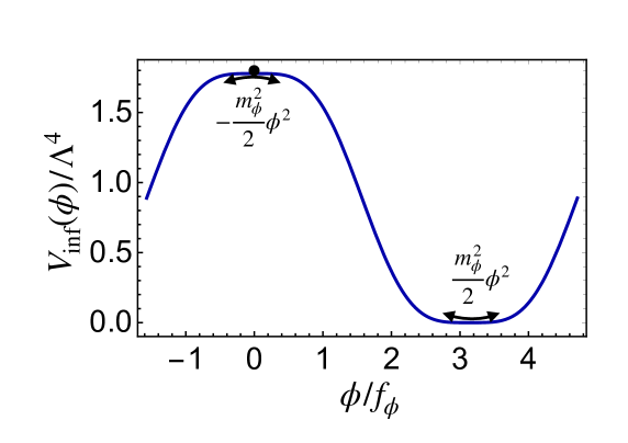
Figure 1: The ALP potential for $n=3$ with $\theta\approx 0$ and $\kappa\approx 1$. The curvatures of the potential at the maximum and minimum are equal to each other but with an opposite sign. The slow-roll inflation takes place around the hilltop of the potential while the ALP excitation around the minimum contributes to DM.

For the moment we set $\theta=0$ and $\kappa=1$ so that the curvature vanishes, $V^{\prime\prime}(0)=0$, at the origin. In this limit, the inflaton dynamics is reduced to the standard hilltop quartic inflation, and the inflaton evolution can be solved analytically. Then, the potential near the origin is approximated by

$$V_{\rm inf}(\phi)\simeq V_{0}-\lambda{\phi^{4}}+\cdots,$$ (2.2)

where we have defined

$$V_{0} \equiv V_{\rm inf}(0)-V_{\rm inf}(\pi f_{\phi})=2{\frac{n^{2}-1}{n^{2}}}\Lambda^{4}$$ (2.3)

$$\lambda \equiv{\frac{n^{2}-1}{4!}}\left({\frac{\Lambda}{f_{\phi}}}\right)^{4}.$$ (2.4)

Here the potential contains no linear or quadratic terms, but the inflaton dynamics is not significantly modified as long as these terms are sufficiently small. In fact, we as shall see shortly, while the hilltop quartic inflation can last sufficiently long to solve the theoretical problems of the standard big bang cosmology, its prediction of the spectral index is too small to explain the observed value. Then, we will introduce linear and quadratic terms as small corrections, which give a better fit to the observed spectral index.

The amplitude of curvature perturbations is calculated from

$$P_{\mathcal{R}}=\left(\frac{H_{\rm inf}^{2}}{2\pi\dot{\phi}_{*}}\right)^{2}\simeq\frac{V_{\rm inf}(\phi_{*})^{3}}{12\pi^{2}V_{\rm inf}^{\prime}(\phi_{*})^{2}M_{p}^{6}},$$ (2.5)

where the subscript $*$ implies that the variable is evaluated at the horizon exit of the pivot scale $k_{*}=0.05{\rm Mpc}^{-1}$. The observed amplitude of the curvature perturbation is given by [26]

$$P_{\mathcal{R}} \simeq 2.1\times 10^{-9}.$$ (2.6)

This fixes the quartic coupling as

$$\lambda\simeq 7.5\times 10^{-14}\left({\frac{N_{*}}{50}}\right)^{-3},$$ (2.7)

where $N_{*}$ is the e-folding number at the horizon exit of the pivot scale.

The scalar spectral index $n_{s}$ is given by

$$n_{s}\simeq 1-6\varepsilon+2\eta,$$ (2.8)

where the slow-roll parameters are defined as

$$\varepsilon(\phi) \equiv\frac{M_{p}^{2}}{2}\left(\frac{V_{\rm inf}^{\prime}}{V_{\rm inf}}\right)^{2},$$ (2.9)

$$\eta({\phi}) \equiv M_{p}^{2}\frac{V_{\rm inf}^{\prime\prime}}{V_{\rm inf}}.$$ (2.10)

Unless the inflation scale is very high, the contribution to $n_{s}$ is known to be dominated by $\eta$. In the hilltop quartic inflation, the inflaton dynamics can be easily solved analytically and one obtains $\eta(\phi_{*})\simeq-3/2N_{*}$, and thus,

$$n_{s}(\phi_{*})\simeq 1-{\frac{3}{N_{*}}}.$$ (2.11)

We are interested in the case of the Hubble parameter during inflation of order keV, which results in $N_{*}=32\,\text{-}\,35$. Then, the predicted value of the spectral index in the quartic hilltop inflation is too small to explain the observed value, $n_{s}=0.9649\pm 0.0044$ [26].

In fact, the spectral index is sensitive to the detailed shape of the inflaton potential, and even a tiny correction can easily modify the predicted value of $n_{s}$ to give a better fit to data. To this end, we introduce a small but nonzero CP phase, $\theta$. For sufficiently small $\theta(>0)$, one can again expand the potential around the origin as

$$V_{\rm inf}(\phi)\simeq V_{0}-\lambda\phi^{4}-\Lambda^{4}\theta\frac{\phi}{f_{\phi}}+\cdots.$$ (2.12)

The linear term can effectively increase the predicted value of $n_{s}$, because, if $\theta>0$, it shifts the inflaton field at the horizon exit of the pivot scale to smaller values where the curvature of the potential, $|V^{\prime\prime}_{\rm inf}|$, is smaller [46]. Note that the linear term does not directly contribute to the $\eta$ parameter. A similar, but slightly weaker effect is obtained by varying the relative height of the potential, $\kappa$, which induces a quadratic term. In fact, if the flatness of the inflaton potential is due to the anthropic selection of the parameters for the inflaton potential, such nonzero values of $\theta$ and $\kappa-1$ may be reasonable because the successful slow-roll inflation only requires a sufficiently flat potential where the slow-roll parameters are smaller than unity.

The inclusion of nonzero $\theta$ and $\kappa-1$ leads to an interesting relation between the mass and the decay constant. From Eq. (2.8), we obtain

$$H_{\rm inf}\approx\sqrt{\frac{V_{0}}{3M_{p}^{2}}}\sim\sqrt{|V_{\rm inf}^{\prime\prime}(\phi_{*})|}\sim\sqrt{|V_{\rm inf}^{\prime\prime}(\phi_{\rm max})|},$$ (2.13)

where we have used in the last equality the fact that $\phi_{*}$ is close to the potential maximum located at $\phi=\phi_{\rm max}$ in the hilltop inflation. Due to the upside-down symmetry, we have

$$m_{\phi}\sim H_{\rm inf},$$ (2.14)

where

$$m_{\phi}\equiv\sqrt{V_{\rm inf}^{\prime\prime}(\phi_{\rm min})}\simeq\left(\frac{9(n^{2}-1)}{2}\right)^{\frac{1}{6}}\theta^{\frac{1}{3}}\frac{\Lambda^{2}}{f_{\phi}}.$$ (2.15)

From (2.7) and (2.14), we arrive at the relation [43, 38, 40, 39]

$$f_{\phi}\sim 10^{3}\sqrt{m_{\phi}M_{p}}.$$ (2.16)

The relation was numerically confirmed in Refs. [38, 39, 40] by solving the inflaton dynamics taking account of higher order corrections to the spectral index. We show in Fig. 2 the numerical result of [40].

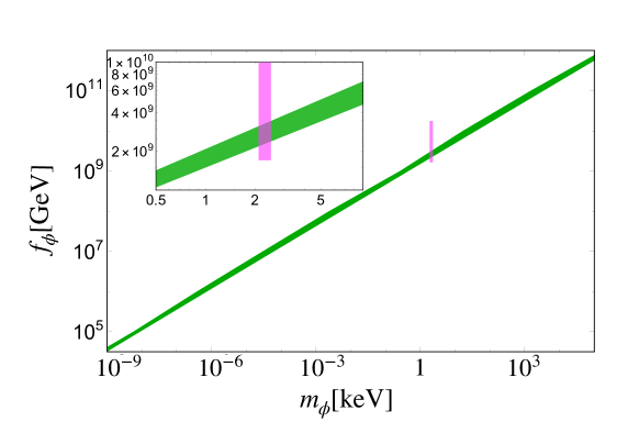
Figure 2: The predicted relation between $m_{\phi}$ and $f_{\phi}$ in the ALP inflation with $n=3$ is shown by the green line, which is adapted from Ref. [40]. The mass and decay constant suggested by the XENON1T excess are shown by the red shaded region for $q_{e}\sqrt{r}=0.1\,\text{-}\,1$. As discussed in the text, the two regions overlap around $q_{e}\sqrt{r}\simeq 0.2$.

For the current purpose we have fitted the numerical results of Ref. [40] for $n=3$ in the range of $10^{9}\ {\rm GeV}\leq f_{\phi}\leq 10^{11}\ {\rm GeV}$ and $|\kappa-1|\lesssim(f_{\phi}/M_{p})^{2},|\theta|\lesssim(f_{\phi}/M_{p})^{3}$ to obtain

$$H_{\rm inf} \simeq(0.1\,\text{-}\,1)\ {\rm keV}\sqrt{\frac{2-2/n^{2}}{16/9}}\left(\frac{f_{\phi}}{10^{9}\ {\rm GeV}}\right)^{2},$$ (2.17)

$$\lambda \simeq(1\,\text{-}\,50)\times 10^{-13}\left(\frac{10^{9}\ {\rm GeV}}{f_{\phi}}\right)^{0.11},$$ (2.18)

where the $n$-dependence is reproduced analytically. Thus we arrive at

$$f_{\phi} \simeq(2\,\text{-}\,4)\times 10^{9}\ {\rm GeV}\left(\frac{n}{3}\right)^{\frac{1}{2}}\left(\frac{m_{\phi}}{2\,{\rm keV}}\right)^{\frac{1}{2}}.$$ (2.19)

One can see that the mass (1.1) and decay constant (1.3) suggested by the XENON1T excess satisfy the relation for $q_{e}\sqrt{r}\sim 0.1$. In the following we take $n=3$, but our results are not so sensitive to the choice of $n$, and the dependence on $n$ can be easily read from Eqs.(2.17), (2.18) and (2.19).

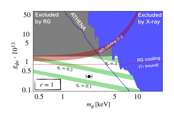
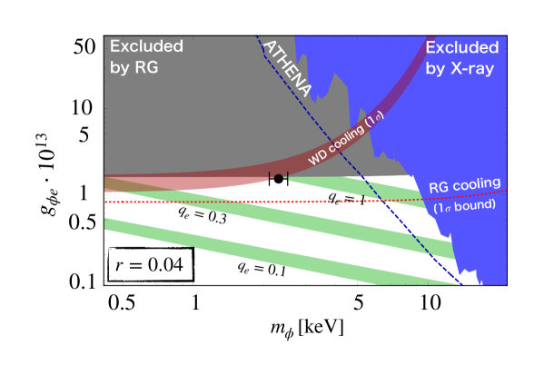
Figure 3: The mass and coupling to electrons suggested by the XENON1T excess are shown by black dots for $r=1$ (upper panel) and $r=0.04$ (lower panel). The predicted relation for $g_{\phi e}$ and $m_{\phi}$ in the ALP inflation is shown as green bands for $q_{e}=1,0.3$, and $0.1$ from top to bottom. The X-ray bound for anomaly-free ALP DM [17, 3] is shown by the blue shaded region. The future sensitivity of ATHENA is shown by the blue dashed line [47, 48]. The red shaded region is preferred by the cooling of white dwarf stars. The gray region and the red dashed line represent the bound from the cooling of the tip of the red-giant branch [25] at $2\sigma$ and $1\sigma$ level, respectively.

In order to take a closer look, we show in Fig. 3 the relation for different values of $q_{e}$ as well as other cosmological and astrophysical constraints. The upper and lower panels are for the fraction of ALP DM, $r=\Omega_{\phi}/\Omega_{\rm DM}=1$ and $0.04$, respectively. The consistency relation (2.19) are shown as green bands for the different PQ charge of electron, $q_{e}=1,0.3$ and $0.1$ from top to bottom. The mass (1.1) and the electron coupling (1.2) suggested by the XENON1T excess are shown as black dots. We can see that, if the ALP DM responsible for the XENON1T excess is the inflaton, the PQ charge of electron and the fraction of ALP DM satisfy

$$q_{e}\sqrt{r}\simeq 0.2.$$ (2.20)

The blue shaded region is excluded by the X-ray observations, and the future sensitivity reach of ATHENA is shown by the blue dashed line [47, 48, 49]. Here we have adopted the decay rate into photons based on the anomaly-free ALP DM model [17, 3]. On the other hand, the cooling argument based on the tip of red-giant branch stars places a tight bound on $g_{\phi e}<1.60\,(0.82)\times 10^{-13}$ at 95$\%$ (68$\%$) CL, and the gray shaded region shows the $2\sigma$ excluded region, and the red dotted line is the 1$\sigma$ bound [25]. The RG cooling bound gives a lower bound on the fraction of ALP DM as $r\gtrsim 0.01$. Note that the red shaded region is favored by the analysis of white dwarf luminosity function [22], which is close to the values suggested by the XENON1T excess especially in the case of $r=0.04$. In the rest of this section we discuss the reheating of the ALP inflation and the abundance of thermally produced ALPs.

2.2 Reheating of the ALP inflation

2.2.1 General argument

After the slow-roll inflation, the ALP (inflaton) starts to oscillate around its potential minimum. The ALP mass at the minimum is of order keV, but it initially has a much larger effective mass, and so, it can efficiently transfer its energy to the SM particles. Here we estimate how efficient the energy transfer should be for successful reheating.

If the ALP couplings to the SM particles are sizable, the reheating completes soon after the onset of oscillations. In other words, the reheating is instantaneous. The reheating temperature in this case is given by

$$T_{R}\simeq(3\,\text{-}\,8)\times 10^{5}{\rm GeV}\left(\frac{g_{*}(T_{R})}{107.75}\right)^{-1/4}\left(\frac{f_{\phi}}{10^{9}\ {\rm GeV}}\right),$$ (2.21)

where we have used (2.17) and set $g_{*}(T_{R})=107.75$ counts all the SM degrees freedom plus thermalized ALP (inflaton) (see later discussion for the thermal production of the ALP). The detailed process of reheating, however, is quite non-trivial because the effective mass of the ALP decreases in time and thermal dissipation processes also play the important role.

Let us approximate the ALP potential around the potential minimum as

$$V(\phi) \simeq\frac{1}{2}m_{\phi}^{2}(\phi-\phi_{\rm min})^{2}+\lambda(\phi-\phi_{\rm min})^{4}.$$ (2.22)

The quadratic term becomes relevant only after the oscillation amplitude of ALP becomes smaller than

$$\phi_{c}=\frac{m_{\phi}}{\sqrt{2\lambda}}.$$ (2.23)

The effective mass of the ALP is approximately given by

$$m_{\rm eff}\simeq\left\{\begin{array}[]{ll}\displaystyle{\sqrt{12\lambda}\,\left|{\phi}\right|}&{\rm for}\left|{\phi}\right|>\phi_{c}\\ &\\ \displaystyle{m_{\phi}}&{\rm for}\left|{\phi}\right|<\phi_{c}\end{array}\right.,$$ (2.27)

where $\left|{\phi}\right|$ is the amplitude of the ALP oscillation. Soon after the onset of oscillations, the effective mass is about $3\ {\rm TeV}$ for $\lambda=10^{-12}$ and $\left|{\phi}\right|=f_{\phi}=10^{9}\ {\rm GeV}$, and it can decay into relatively heavy SM particles. The decay products quickly thermalize and form thermal plasma. Because of the time-dependent effective mass, however, the perturbative decay stops at a certain point, and afterwards the dominant reheating process is taken over by thermal dissipation process. If the dissipation process is efficient, the ALP condensate will evaporate completely. If not, there may remain some amount of the ALP condensate which contributes to DM. In the former case, the ALP is considered to be thermalized, which we will discuss later in this section.

We denote the fraction of the remnant of the ALP condensate by $\xi$:

$$\xi\equiv\left.\frac{\rho_{\phi}}{\rho_{\phi}+\rho_{R}}\right|_{\rm after\,reheating},$$ (2.28)

where $\rho_{\phi}$ and $\rho_{R}$ are the energy density of the ALP condensate and radiation, respectively, and $\xi$ is defined just after the reheating (decay or dissipation) becomes ineffective. The precise value of $\xi$ can be estimated by numerically solving the Boltzmann equation for given interactions. Here let us estimate how small $\xi$ should be for successful reheating.

The amplitude of the ALP oscillations after the reheating is about $\xi^{\frac{1}{4}}f_{\phi}$ since the initial amplitude is of order $f_{\phi}$. Then, the ALP energy density to entropy ratio is given by

$$\frac{\rho_{\phi}}{s} \simeq\frac{3}{4}\Delta\xi^{\frac{3}{4}}\frac{m_{\phi}T_{R}}{\sqrt{2\lambda}f_{\phi}},$$ (2.29)

where we have introduced an entropy dilution factor $\Delta(<1)$ for later purpose. Using Eqs. (2.18) and (2.21), we obtain

$$\xi\sim 10^{-4}\times\left(\frac{10^{-3}}{\Delta}\right)^{4/3}\left(\frac{2\ {\rm keV}}{m_{\phi}}\right)^{4/3}\left(\frac{\Omega_{\rm\phi}h^{2}}{0.12}\right)^{4/3}\left(\frac{f_{\phi}}{10^{9}\ {\rm GeV}}\right)^{-0.073}.$$ (2.30)

Since the ALP relic density should not exceed the observed DM density, $\Omega_{\rm\phi}h^{2}\lesssim 0.12$, we have an upper bound on $\xi$. If there were not for any entropy dilution (i.e. $\Delta=1$), $\xi$ should be smaller than $10^{-8}$, and in the presence of the entropy dilution of $10^{-3}$, it should be smaller than $10^{-4}$.

2.2.2 Specific examples of the ALP couplings

Now we specify interactions between the ALP and SM particles to estimate $\xi$. As we consider the anomaly-free ALP model where the continuous shift symmetry (PQ symmetry) of $\phi$ is not broken by the interactions with the SM particles, the relevant interactions are given by the following derivative couplings with SM fermions

$${\cal L}^{\rm int}_{\rm eff}=C_{ij}\frac{\partial_{\mu}\phi}{2f_{\phi}}\bar{\psi}_{i}\gamma_{5}\gamma^{\mu}{\psi}_{j}+{\cal O}(1/f_{\phi}^{2}),$$ (2.31)

where $\psi_{i}$ represents the SM fermion with a flavor index $i$ running over $i=e,\mu,\tau,u,d,s,\cdots$, and $C_{ij}$ is a Hermitian matrix representing the ALP coupling. Note that there are no anomalous couplings to the SM gauge bosons by definition of the anomaly-free ALP. We have also concentrated on the CP-conserving interactions for simplicity.

By performing field redefinition, we can rewrite the derivative couplings in terms of the Yukawa couplings,

$${\cal L}_{\rm Yukawa}=\frac{ig_{\phi{ij}}}{v}\phi\left(\bar{\psi_{i}}\gamma_{5}H\psi_{j}\right)$$ (2.32)

with $g_{\phi ij}=(y^{\dagger}_{\psi}\cdot C+C\cdot y_{\psi})_{ij}\,v/(2f_{\phi})$, where $y_{\psi}$ represents the Yukawa matrices, $v\approx 174\rm\,GeV$ is the Higgs vacuum expectation value (VEV), and $H$ should be replaced with $\tilde{H}=i\sigma_{2}H^{*}$ for up-type quarks. We also dropped the term of ${\cal O}((\phi/f_{\phi})^{2})$. The electron coupling is given by $g_{\phi e}\equiv g_{\phi ee}$ in this notation. In this basis, anomalous couplings to the SM gauge bosons may or may not be induced by the change of path-integral measure when one performs the field redefinition from (2.31) to (2.32). Whether an anomalous coupling appears depends on the nature of the PQ current in (2.31), and therefore on the UV origin of the anomaly-free PQ symmetry. For instance, if the PQ anomaly is cancelled among the contributions of the SM fermions, in other words, the PQ current in (2.31) is anomaly-free, the anomalous coupling does not appear above the EW scale in the basis of (2.32). This is the case of the lepton specific [17, 3] or the two-Higgs doublet [40, 3] model. On the other hand, if the anomaly is cancelled between the SM fermions and a PQ fermion which may be as heavy as the PQ scale, there appear anomalous couplings below the PQ scale in (2.32). The couplings are originated from the triangle diagram contributions of integrating out the PQ fermion. When we further integrate out all the SM fermions to see the physics at around keV scales, the anomalous couplings will be cancelled out.

With any UV completion, we can move to the basis where ALP couples to fermions only via derivative couplings as (2.31). In this basis, there should not be any additional anomalous couplings to photons or gluons since the ALP is anomaly-free to them. By integrating out the fermions in the effective Lagrangian (2.31), the ALP-photon coupling is generated accompanied with the derivatives of $\phi$, e.g. $\partial^{2}\phi F\tilde{F}$, thanks to the shift symmetry. Since the electron is the lightest charged fermion, the dominant photon coupling is Eq. (1.4) unless $q_{e}$ is highly suppressed compared with the PQ charge for the other fermions [17, 3] (see also Ref. [16]).

Now let us discuss reheating in this set-up. In the Yukawa basis we generically have two sources for the reheating, the couplings to fermions and to gauge bosons. In fact, even if the anomalous couplings are present in the Yukawa basis, the reheating process via the anomalous couplings turns out to be negligible in the parameter space under consideration [38, 39]. Thus, in the following we discuss the reheating process through Eq. (2.32). To simplify the discussion, we consider flavor-diagonal couplings

$$C_{ij}=q_{i}\delta_{ij},~{}~{}y_{\psi}=\delta_{ij}y_{\psi_{i}},$$ (2.33)

and we neglect the off-diagonal components of the Yukawa matrices.

The ALP decays into two fermions, $\phi\rightarrow\psi_{i}+\bar{\psi}_{i}$, with the decay rate of

$$\Gamma_{{\rm dec},\psi}\simeq\frac{n_{c}}{8\pi}\left(\frac{q_{i}m_{\psi_{i}}}{f_{\phi}}\right)^{2}m_{\rm eff},$$ (2.34)

if the mass or thermal mass of $\psi$ is smaller than the effective mass of the ALP. On the other hand, if the thermal mass of $\psi$ exceeds $m_{\rm eff}$, namely $eT\gtrsim m_{\rm eff}$ (or $g_{s}T\gtrsim m_{\rm eff}$), the decay process stops and the dissipation process such as $\phi+\psi_{i}\rightarrow\psi_{i}+\gamma\,({\rm or~{}}g)$ becomes relevant. The dissipation rate is given by [52]

$$\Gamma_{{\rm dis},\psi}\simeq\displaystyle{A_{0}n_{c}\left(\frac{q_{i}m_{\psi_{i}}}{f_{\phi}}\right)^{2}\left(\frac{\alpha_{\psi}}{2\pi^{2}}\right)T,}$$ (2.35)

for $T<T_{\rm EW}$, where $T_{\rm EW}$ is the temperature of the electroweak phase transition, $A_{0}$ ($\simeq 0.5$) is a numerical constant, $\alpha_{\psi}$ is the fine-structure constant of the relevant gauge coupling, $e$ (or $g_{s}$). Before the electroweak phase transition, on the other hand, the dissipation proceeds via the interaction with the Higgs field such as $\phi+{\rm Higgs}\rightarrow\psi_{i}+\bar{\psi}_{i}$. Then the dissipation rate is given by [39, 53]

$$\Gamma_{{\rm dis},H}\simeq n_{c}\left(\frac{q_{i}^{2}y_{\psi_{i}}^{2}}{2\pi^{3}f_{\phi}^{2}}\right)T^{3},$$ (2.36)

for $T>T_{\rm EW}$. Note that, while the perturbative decay gradually becomes inefficient as the effective mass decreases in time, the dissipation rate of (2.36) and (2.35) is independent of $m_{\rm eff}$, and so, it is efficient until the ALP disappears completely.

Now we can calculate the fraction of the relic ALP condensate $\xi$ by solving the Boltzmann equations of

$$\left\{\begin{array}[]{ll}\displaystyle{\dot{\rho}_{\phi}+4H\rho_{\phi}=-\Gamma_{\rm tot}\rho_{\phi}}\\ &\\ \displaystyle{\dot{\rho}_{r}+4H\rho_{r}=\Gamma_{\rm tot}\rho_{\phi}}\end{array}\right.,$$ (2.40)

where $\Gamma_{\rm tot}=\Gamma_{{\rm dec},\psi}+\Gamma_{{\rm dis},\psi(H)}$. Since $\Gamma_{{\rm dis},\psi H}/H$ is larger for higher $T$, we find that the dissipation effect is most efficient just after the inflation ends. This implies that the remnant fraction of the ALP condensate is exponentially suppressed as

$$\xi\propto\exp\left[-\Gamma_{{\rm dis},H}/H\right]$$ (2.41)

with

$$\frac{\Gamma_{{\rm dis},H}}{H} \simeq n_{c}\left(\frac{q_{i}^{2}y_{\psi_{i}}^{2}}{2\pi^{3}}\right)\sqrt{\frac{90}{\pi^{2}g_{*}(T_{R})}}\frac{T_{R}M_{p}}{f_{\phi}^{2}}$$ (2.42)

$$\simeq 10^{4}\times n_{c}q_{i}^{2}y_{\psi_{i}}^{2}\left(\frac{T_{R}}{10^{6}\ {\rm GeV}}\right)\left(\frac{f_{\phi}}{10^{9}\ {\rm GeV}}\right)^{-2}\left(\frac{g_{*}(T_{R})}{107.75}\right)^{-1/2}.$$ (2.43)

Thus the remnant of the ALP inflaton is negligibly small if $n_{c}q_{i}^{2}y_{\psi_{i}}^{2}\gtrsim 10^{-3}$. For $q_{i}={\cal O}(0.1\,\text{-}\,10)$, $\xi$ becomes sufficiently small and the reheating will be successful if the $i$ contains (relatively) heavy fermions such as $\tau,b,c$ or $t$.

We have numerically solved the Boltzmann equation and find that the reheating becomes inefficient and $\xi\approx 1$ for $n_{c}q_{i}^{2}y_{\psi_{i}}^{2}\ll 10^{-3}$ and $f_{\phi}\sim 10^{9}\,$GeV, even if we take into account the dissipation effect of Eq. (2.35) and the perturbative decays at a later time. For $n_{c}q_{i}^{2}y_{\psi_{i}}^{2}\gtrsim 10^{-3}$, we have confirmed that $\xi$ is exponentially suppressed and the reheating completes instantaneously. The reheating temperature is therefore given by Eq. (2.21).

In summary, if the XENON1T excess is explained by the ALP DM which drives inflation in the early universe, the ALP must be coupled to heavy fermions for successful reheating. The reheating is almost instantaneous, and the reheating temperature is of order $10^{6}$ GeV.

2.3 Thermal production of ALP

The ALP can also be produced from thermal plasma through the inverse process of the diffusion effect. Since the diffusion effect is efficient for the successful reheating, the ALP is always thermally populated. This is a rather robust prediction of our scenario. The thermally produced ALP can be the potential source of the XENON1T excess.

The abundance of the thermally produced ALP is given by

$$\Omega_{\phi}^{\rm(th)}h^{2}\simeq 2.1\Delta\left(\frac{m_{\phi}}{2\ {\rm keV}}\right)\left(\frac{g_{*s}}{106.75}\right),$$ (2.44)

where $g_{*s}$ is the relativistic degrees of freedom for entropy density of the SM particles and we have included the entropy dilution factor $\Delta(<1)$. In order not to exceed the observed DM abundance for $\Delta=1$, the thermally produced ALP must be diluted by some late-time entropy production. The required amount of the entropy dilution factor is given by

$$\Delta\simeq 0.06\left(\frac{\Omega_{\phi}^{\rm(th)}h^{2}}{0.12}\right),$$ (2.45)

where we used $m_{\phi}\simeq 2\ {\rm keV}$. In the next section we will discuss such entropy production mechanism.

Lastly, we note that a thermally produced ALP with a keV-scale mass has a nonzero free-streaming velocity at the structure formation, and it behaves as warm DM. The Lyman-$\alpha$ observation puts an upper bound on the free-streaming velocity, which can be translated to the upper bound on the mass of the warm DM for a given momentum distribution. In the case of the sterile neutrino, its mass is bounded as $m_{\nu_{s}}>5.3$ keV [54, 55] if it constitutes the dominant DM. The bound on the ALP warm DM should be of the same order, although the degree of freedom and the statistics are different. Also, there are constraints from observations of CMB, the baryon acoustic oscillation (BAO) and the number of dwarf satellite galaxies in the Milky Way [56], which imply that the ALP warm DM with mass of $2$ keV is likely in a tension with observations. One way to relax the tension is to consider a case that the ALP occupies only a fraction of DM. Indeed, if $r<0.1$, the constraints are significantly relaxed. To explain the XENON1T excess, we need $r>0.01$ (see Fig. 3). Therefore, our scenario may be tested if the aforementioned bounds for the warm DM are improved [57, 58, 59, 60].

If the thermally produced ALP constitutes only a fraction of DM, the dominant component may come from the remnant of the inflaton condensate via incomplete reheating (see (2.30)). This is the case if $n_{c}q_{i}^{2}y_{\psi_{i}}^{2}\sim 10^{-3}$. On the other hand, the dominant DM component may be another axion(s). As we will discuss later, there may be many axions in nature as in the axiverse scenario, and then, $m_{\phi}\sim H_{\rm inf}\sim$ keV may be explained by the anthropic argument based on the initial axion amplitude and the abundance.

3 Entropy dilution and leptogenesis

It is natural to introduce right-handed neutrinos to explain the smallness of the active neutrino masses by the seesaw mechanism and to produce baryon asymmetry via leptogenesis. The Lagrangian is written as

$${\cal L}_{N_{R}}=({\rm kineticterms})-\frac{1}{2}M_{i}\bar{N^{c}_{i}}N_{i}-y_{ij}^{\nu}\bar{L}_{j}H\hat{P}_{R}N_{i}+{\rm h.c.},$$ (3.1)

where $L_{j}$ is a left-handed Lepton field in the chiral representation. As we will see shortly, the decay of right-handed neutrinos can result in an entropy dilution that is required in our scenario.

The right-handed neutrino, $N_{i}$ is also produced through the inflaton decay if it is lighter than $m_{\rm eff}$ and has derivative couplings like

$${\cal L}^{\rm int}_{\rm eff}\supset C_{N_{i}N_{j}}\frac{\partial_{\mu}\phi}{2f_{\phi}}\bar{N_{i}}\gamma_{5}\gamma^{\mu}{N_{j}}.$$ (3.2)

In the mass basis, we obtain,

$${\cal L}_{\rm mass}=iC_{N_{i}N_{j}}(M_{i}+M_{j})\frac{\phi}{2f_{\phi}}\bar{N^{c}_{i}}\gamma_{5}N_{j}.$$ (3.3)

We have ignored the ALP coupling via Yukawa interactions in Eq. (3.1) since $y^{\nu}_{ij}$ is small in the parameter region of our interest.

In particular, the right-handed neutrino, $N_{1}$, corresponding to the lightest active neutrino, can be produced. The number density of $N_{1}$ to entropy density ratio is given as

$$\frac{n_{N}}{s}\sim\frac{3}{4}\frac{T_{R}}{m_{\rm eff}/2}\frac{\Gamma_{\phi\to N_{1}N_{1}}}{\Gamma_{\rm tot}}\sim 7\frac{C_{N_{1}N_{1}}^{2}M_{1}^{2}}{n_{c}(q_{i}y_{\psi_{i}})^{2}T_{R}^{2}}.$$ (3.4)

This takes the maximum value of ${\cal O}$($10^{-3}$), when $M_{1}\sim m_{\rm eff}$ and $n_{c}(y_{\psi_{i}}q_{i})^{2}\sim 10^{-3}$. The right-handed neutrino comes to dominate the Universe when the temperature decreases to

$$T_{\rm dom}\simeq\frac{4}{3}M_{1}\frac{n_{N}}{s}\sim 10\ {\rm GeV}\left(\frac{10^{-3}}{n_{c}(y_{\psi_{i}}q_{i})^{2}/C_{N_{1}N_{1}}^{2}}\right)\left(\frac{10^{6}\ {\rm GeV}}{T_{R}}\right)^{2}\left(\frac{M_{1}}{10^{3}\ {\rm GeV}}\right)^{3}.$$ (3.5)

Then $N_{1}$ decays into the SM particles to reheat the universe with a temperature $T=T_{N}$. The ALP-number-to-entropy ratio after the decay of $N_{1}$ is given as

$$\left.\frac{n_{\phi}}{s}\right|_{T=T_{N}}=\left.\frac{n_{N}}{s}\right|_{T=T_{N}}\left.\frac{n_{\phi}}{n_{N}}\right|_{T=T_{\rm dom}}=\frac{T_{N}}{T_{\rm dom}}\left.\frac{n_{\phi}}{s}\right|_{T=T_{\rm dom}}.$$ (3.6)

Thus, we identify the dilution factor as $\Delta=T_{N}/T_{\rm dom}.$ The right-handed neutrino should decay before the big bang nucleosynthesis (BBN), $T_{N}\gtrsim 1\ {\rm MeV}$, not to spoil the successful prediction of the light element abundances [61, 62, 63, 64, 65, 66, 67]. Then, the dilution factor is bounded below

$$10^{-4}\left(\frac{10\ {\rm GeV}}{T_{\rm dom}}\right)\lesssim\Delta\leq 1,$$ (3.7)

which in turn implies that the abundance of the thermally produced ALP is in the range of

$$\Omega_{\phi}^{\rm(th)}=O(10^{-3}\,\text{-}\,1).$$ (3.8)

This has a large overlap with the range of $r$ where the XENON1T excess can be explained (see Fig. 3).

Let us mention a possible baryogenesis associated with the right-handed neutrinos. In the case of $1\,{\rm TeV}\lesssim M_{2}\approx M_{3}\lesssim 10^{6}\ {\rm GeV}$, the right amount of baryon asymmetry can be generated via resonant leptogenesis [68, 69], though thermal leptogenesis [70] is difficult because of the low reheating temperature $T_{R}\sim 10^{6}\ {\rm GeV}$. On the other hand, in the case of $M_{2,3}\sim 1\,\text{-}\,100\rm\,GeV$, the baryon asymmetry can be obtained from the flavor oscillation of the left-handed leptons which are produced from the inflaton decay if the ALP-lepton derivative couplings are flavor-violating and are not too small [71, 72]. Note that generated baryon asymmetry is also diluted by the entropy production of $N_{1}$, and one needs to generate larger baryon asymmetry by a factor of $\Delta^{-1}$ than the observed value.

Another way to have late-time entropy production is to introduce a B$-$L Higgs field. The U(1)_B-L gauge symmetry is assumed to be restored after inflation, and the B$-$L Higgs field stays at the origin and dominates the universe for a while. After the symmetry breaking, the B$-$L Higgs decays into the SM particles and produce entropy that leads to $\Delta\sim{\cal O}(0.01\,\text{-}\,0.1)$. See Appendix for the estimation of the dilution factor in this scenario. In this case the right-handed neutrino can be produced efficiently in the symmetric phase through the U(1)_B-L gauge interactions. The decays of the right-handed neutrinos can generate baryon asymmetry via resonant leptogenesis.

4 Discussion

So far we have considered a single-field inflation model, but the ALP inflation can be extended to multi-field inflation where the two axions respectively play the role of the inflaton and waterfall field as in the hybrid inflation [38] (see also Refs. [74, 75]). Even in this case, the consistency relation between the mass and decay constant is known to hold, while the reheating process can be quite different [38]. It may be able to induce the entropy production from one axion while the other becomes DM and explains the XENON1T excess.

In our scenario, the inflation scale is predicted to be around $H_{\rm inf}\sim 1\,$keV. Since this is lower than the QCD scale, if the QCD axion, $a$, exists to solve the strong CP problem, it acquires a potential via the non-perturbative effect during inflation. In the ALP inflation model considered in the text, the eternal inflation can take place around the potential maximum. If the inflation lasted sufficiently long, then the QCD axion field follows an equilibrium probability distribution peaked around the CP-conserving minimum with a variance $\sim 0.1H_{\rm inf}^{2}(m_{a}f_{a})^{-1}$ due to the stochastic process, where $m_{a}~{}{\rm and}~{}f_{a}$ are the QCD axion mass and decay constant, respectively. The resulting abundance of the QCD axion is highly suppressed [76, 77].

Here let us comment on a possibility that the ALP mass is determined by the anthropic principle [82, 83, 84, 85, 86]. In the string axiverse, there are many ALPs with the decay constants of order $10^{16}\ {\rm GeV}$ [87, 88]. We expect that the masses of these ALPs are logarithmically distributed over a wide range of energy scales, because their masses are generated by non-perturbative effects. Then, while heavy ALPs already settle down at their potential minimum during inflation, light ALPs may start to oscillate coherently around their potential minimum after inflation. The energy densities of the coherent oscillations behave like DM.

Now we shall take into account the anthropic condition on the DM abundance. If the DM is too abundant, the cosmological structure would be significantly complicated, and the number of small-scale structure, like galaxies, might become quite large. As a result, the collision rate of stars/comets may be too large and there may be no time for sapient life to emerge on a planet like the Earth. The consideration along this line puts an upper bound on the DM abundance, which turns out to be larger than the observed DM abundance, but not by many orders of magnitude. (see, e.g., Ref. [89]). Then, the energy densities of the ALP coherent oscillations must be suppressed to satisfy the anthropic condition on the DM abundance.

One might think that the initial misalignment angle of each ALP can be fine-tuned to satisfy the anthropic condition. However, the total amount of fine-tuning would be very large if there are many ALPs, and it depends on which parameters are actually environmental parameters whether such tuning is justified. Instead, we consider the case in which the anthropic condition is satisfied by varying the Hubble parameter during inflation, namely $H_{\rm inf}$. In Ref. [90], Ho and two of the present authors (FT and WY) studied the stochastic behavior of string axions and showed that the abundance of the ALP coherent oscillations is sufficiently suppressed if $H_{\rm inf}\lesssim{\cal O}(1)\ {\rm keV}$ for the ALP decay constants of order $10^{16}\ {\rm GeV}$. Therefore, if $H_{\rm inf}$ is randomly distributed in the string landscape and is biased toward a larger value, $H_{\rm inf}={\cal O}(1)\ {\rm keV}$ is chosen by the anthropic condition on the DM abundance. Noting that the mass of the inflaton ALP is of the same order with $H_{\rm inf}$ in our scenario, this is another interesting coincidence with the XENON1T excess.

Lastly let us comment on a possibility of the PQ symmetry restoration. In the main text we have focused on the case that the PQ symmetry is already broken during inflation as the inflaton was identified with the corresponding ALP. In a more general case where the ALP is not necessarily the inflaton, the PQ symmetry could be restored in the early universe and gets spontaneously broken some time after inflation. This scenario has advantages; the ALP has no isocurvature perturbation, and the inflation scale can be high; also, the reheating temperature (of the SM sector) can be high which makes it easier to generate the right amount of baryon asymmetry. The cosmic strings and domain walls are formed after the phase transition, but they will disappear if the corresponding domain wall number is equal to unity, namely if there is a unique vacuum. On the other hand, we need to make sure that the ALP is not thermalized, since its abundance would be larger than the observed DM abundance and some entropy dilution would be required. In particular, if the PQ sector including the PQ scalar(s) are thermalized, the ALP is expected to be already thermally populated right after the phase transition. In the simplest case with a single PQ complex scalar, the thermalized real and imaginary components will become the radial direction of the PQ-symmetry breaking field and ALP after the phase transition. One way to avoid the overproduction of the ALP is to assume that the PQ sector has been always decoupled from the SM sector, and it is never thermalized. Then, the timing of the PQ phase transition is model-dependent, and it depends on e.g. the detailed shape of the potential for the PQ scalar, or the interactions among the PQ scalars. If the phase transition takes place at a late time, the temperature of the SM sector can be so low that thermal production of the ALPs becomes negligibly small. In an extreme case in which the PQ sector has a clockwork structure, the phase transition indeed takes place at a very late time, and the resultant topological defects have a complicated structure [91, 92, 93]. Note, however, that the radial direction of the PQ-symmetry breaking field should dominantly decay to the SM particles so that hot/warm ALP is not overproduced [94].

5 Conclusions

In this paper we have pointed out that, when the XENON1T excess is interpreted in terms of the ALP dark matter, the suggested mass and decay constant agree very well with the relation of (1.5) that is predicted in the ALP inflation model. The relation was derived solely based on the CMB normalization and the scalar spectral index. For the mass and decay constant suggested by the XENON1T excess, the Hubble parameter during inflation is predicted to be $H_{\rm inf}\sim\ {\rm keV}.$ If the ALP is coupled to relatively heavy SM fermions, the reheating proceeds almost instantaneously and the reheating temperature is given by $T_{R}\sim 10^{6}\ {\rm GeV}$.

After the reheating, the ALP is produced from the scattering in the thermal plasma. The thermally produced ALP DM explains the XENON1T excess once its abundance is diluted by a factor of $10$. Such a mild entropy dilution can be realized in simple cosmological scenarios. We have presented a scenario where the inflaton decays into right-handed neutrinos, and the lightest right-handed neutrino can dominate and reheat the Universe to produce the entropy. Our scenario have various implications for small-scale structure as well as lepton flavor violation. Future observations of 21 cm lines, CMB, BAO, dwarf galaxies and $\mu\to e+$ missing will provide us with further information on the possible relation between DM and inflation.

Appendix A Entropy dilution by thermal inflation

Here we discuss another possible source of entropy dilution. Suppose that there is U(1)_B-L gauge symmetry, which is spontaneously broken at an intermediate scale to give a nonzero mass for the right-handed neutrino. We assume that the U(1)_B-L breaking field $\Psi$ has the Higgs-like potential such as

$$V(|\Psi|)=\lambda_{\Psi}\left(\left|{\Psi}\right|^{2}-\frac{1}{2}v_{\Psi}^{2}\right)^{2}+V_{T}(\Psi)\,.$$ (A.1)

Here, we include the thermal potential $V_{T}$, which is given by

$$V_{T}(|\Psi|)=\left(\frac{\lambda_{\Psi}}{3}+q_{\Psi}^{2}\frac{g^{2}}{4}\right)T^{2}\left|{\Psi}\right|^{2}\,,$$ (A.2)

where $q_{\Psi}$ ($g$) is the U(1)_B-L charge (gauge coupling) of $\Psi$. The critical temperature, below which the U(1)_B-L Higgs field has a nonzero VEV, is then given by

$$T_{c}=\sqrt{\frac{\lambda_{\Psi}}{\lambda_{\Psi}/3+q_{\Psi}^{2}g^{2}/4}}\,v_{\Psi}\,.$$ (A.3)

The entropy is released from the decay of the U(1)_B-L Higgs field. We define a dilution factor as the ratio of the final to the initial comoving entropy density as

$$\Delta^{-1}\equiv\frac{s_{i}a_{i}^{3}}{s_{f}a_{f}^{3}}=1+\frac{4}{3}\frac{g_{*s}(T_{\rm RH,\Psi})}{g_{*}(T_{\rm RH,\Psi})\,T_{\rm RH,\Psi}}\frac{V(0)}{(2\pi^{2}/45)\,g_{*s}(T_{c})\,T_{c}^{3}}\,,$$ (A.4)

where $g_{*s}$ ($g_{*}$) is the effective number of relativistic degrees of freedom for entropy (energy) density as a function of $T$. Here, $V(0)=\lambda_{\Psi}v_{\Psi}^{4}/4$, and $a_{i}$ ($a_{f}$) is the scale factor and $s_{i}$ ($s_{f}$) is the entropy density before (after) the thermal inflation. If the reheating completes instantaneously, the reheating temperature is given by

$$T_{\rm RH,\Psi}=\left(\frac{30V(0)}{g_{*}(T_{\rm RH,\Psi})\,\pi^{2}}\right)^{1/4}.$$ (A.5)

Then, we obtain

$$\Delta\simeq 0.06\times(q_{\Psi}g)^{-3}\left(\frac{g_{*s}(T_{c})\lambda_{\Psi}}{10^{-3}}\right)^{3/4},$$ (A.6)

where we have assumed $g_{*s}(T_{\rm RH,\Psi})=g_{*}(T_{\rm RH,\Psi})$, $\Delta\ll 1$, and $\lambda_{\Psi}\ll q_{\Psi}^{2}g^{2}$. For instance, if we take a value of $\lambda_{\Psi}\lesssim g^{4}q_{\Psi}^{4}/16\pi^{2}$ which is slightly smaller than the natural value determined by the radiative correction, we obtain $\Delta\lesssim{\cal O}(1)$. Therefore, with a mild tuning of the $\lambda$ with respect to the Coleman-Weinberg set-up, $\Delta$ can be of order $0.01-0.1$.

References

- [1] XENON collaboration, E. Aprile et al., Observation of Excess Electronic Recoil Events in XENON1T, 2006.09721.
- [2] M. Szydagis, C. Levy, G. Blockinger, A. Kamaha, N. Parveen and G. Rischbieter, Investigating the XENON1T Low-Energy Electronic Recoil Excess Using NEST, 2007.00528.
- [3] F. Takahashi, M. Yamada and W. Yin, XENON1T anomaly from anomaly-free ALP dark matter and its implications for stellar cooling anomaly, 2006.10035.
- [4] I. M. Bloch, A. Caputo, R. Essig, D. Redigolo, M. Sholapurkar and T. Volansky, Exploring New Physics with O(keV) Electron Recoils in Direct Detection Experiments, 2006.14521.
- [5] P. Athron et al., Global fits of axion-like particles to XENON1T and astrophysical data, 2007.05517.
- [6] J. Jaeckel and A. Ringwald, The Low-Energy Frontier of Particle Physics, Ann. Rev. Nucl. Part. Sci. 60 (2010) 405 [1002.0329].
- [7] A. Ringwald, Exploring the Role of Axions and Other WISPs in the Dark Universe, Phys. Dark Univ. 1 (2012) 116 [1210.5081].
- [8] P. Arias, D. Cadamuro, M. Goodsell, J. Jaeckel, J. Redondo and A. Ringwald, WISPy Cold Dark Matter, JCAP 1206 (2012) 013 [1201.5902].
- [9] P. W. Graham, I. G. Irastorza, S. K. Lamoreaux, A. Lindner and K. A. van Bibber, Experimental Searches for the Axion and Axion-Like Particles, Ann. Rev. Nucl. Part. Sci. 65 (2015) 485 [1602.00039].
- [10] D. J. E. Marsh, Axion Cosmology, Phys. Rept. 643 (2016) 1 [1510.07633].
- [11] I. G. Irastorza and J. Redondo, New experimental approaches in the search for axion-like particles, Prog. Part. Nucl. Phys. 102 (2018) 89 [1801.08127].
- [12] L. Di Luzio, M. Giannotti, E. Nardi and L. Visinelli, The landscape of QCD axion models, 2003.01100.
- [13] G. Alonso-Álvarez, F. Ertas, J. Jaeckel, F. Kahlhoefer and L. J. Thormaehlen, Hidden Photon Dark Matter in the Light of XENON1T and Stellar Cooling, 2006.11243.
- [14] K. Nakayama and Y. Tang, Gravitational Production of Hidden Photon Dark Matter in light of the XENON1T Excess, 2006.13159.
- [15] H. An, M. Pospelov, J. Pradler and A. Ritz, New limits on dark photons from solar emission and keV scale dark matter, 2006.13929.
- [16] M. Pospelov, A. Ritz and M. B. Voloshin, Bosonic super-WIMPs as keV-scale dark matter, Phys. Rev. D78 (2008) 115012 [0807.3279].
- [17] K. Nakayama, F. Takahashi and T. T. Yanagida, Anomaly-free flavor models for Nambu–Goldstone bosons and the 3.5keV X-ray line signal, Phys. Lett. B734 (2014) 178 [1403.7390].
- [18] K. Nandra et al., The Hot and Energetic Universe: A White Paper presenting the science theme motivating the Athena+ mission, 1306.2307.
- [19] Lynx Team collaboration, The Lynx Mission Concept Study Interim Report, 1809.09642.
- [20] eXTP collaboration, S. N. Zhang et al., eXTP – enhanced X-ray Timing and Polarimetry Mission, Proc. SPIE Int. Soc. Opt. Eng. 9905 (2016) 99051Q [1607.08823].
- [21] e-ASTROGAM collaboration, M. Tavani et al., Science with e-ASTROGAM: A space mission for MeV–GeV gamma-ray astrophysics, JHEAp 19 (2018) 1 [1711.01265].
- [22] M. M. Miller Bertolami, B. E. Melendez, L. G. Althaus and J. Isern, Revisiting the axion bounds from the Galactic white dwarf luminosity function, JCAP 1410 (2014) 069 [1406.7712].
- [23] A. H. Córsico, A. D. Romero, L. G. Althaus, E. García-Berro, J. Isern, S. O. Kepler et al., An asteroseismic constraint on the mass of the axion from the period drift of the pulsating DA white dwarf star L19-2, JCAP 1607 (2016) 036 [1605.06458].
- [24] N. Viaux, M. Catelan, P. B. Stetson, G. Raffelt, J. Redondo, A. A. R. Valcarce et al., Neutrino and axion bounds from the globular cluster M5 (NGC 5904), Phys. Rev. Lett. 111 (2013) 231301 [1311.1669].
- [25] F. Capozzi and G. Raffelt, Axion and neutrino red-giant bounds updated with geometric distance determinations, 2007.03694.
- [26] Planck collaboration, Y. Akrami et al., Planck 2018 results. X. Constraints on inflation, 1807.06211.
- [27] A. H. Guth, The Inflationary Universe: A Possible Solution to the Horizon and Flatness Problems, Phys. Rev. D23 (1981) 347.
- [28] A. A. Starobinsky, A New Type of Isotropic Cosmological Models Without Singularity, Phys. Lett. 91B (1980) 99.
- [29] K. Sato, First Order Phase Transition of a Vacuum and Expansion of the Universe, Mon. Not. Roy. Astron. Soc. 195 (1981) 467.
- [30] A. D. Linde, A New Inflationary Universe Scenario: A Possible Solution of the Horizon, Flatness, Homogeneity, Isotropy and Primordial Monopole Problems, Phys. Lett. 108B (1982) 389.
- [31] A. Albrecht and P. J. Steinhardt, Cosmology for Grand Unified Theories with Radiatively Induced Symmetry Breaking, Phys. Rev. Lett. 48 (1982) 1220.
- [32] K. Freese, J. A. Frieman and A. V. Olinto, Natural inflation with pseudo - Nambu-Goldstone bosons, Phys. Rev. Lett. 65 (1990) 3233.
- [33] N. Arkani-Hamed, H.-C. Cheng, P. Creminelli and L. Randall, Extra natural inflation, Phys. Rev. Lett. 90 (2003) 221302 [hep-th/0301218].
- [34] M. Czerny and F. Takahashi, Multi-Natural Inflation, Phys. Lett. B733 (2014) 241 [1401.5212].
- [35] M. Czerny, T. Higaki and F. Takahashi, Multi-Natural Inflation in Supergravity and BICEP2, Phys. Lett. B734 (2014) 167 [1403.5883].
- [36] D. Croon and V. Sanz, Saving Natural Inflation, JCAP 1502 (2015) 008 [1411.7809].
- [37] T. Higaki and F. Takahashi, Elliptic inflation: interpolating from natural inflation to R2-inflation, JHEP 03 (2015) 129 [1501.02354].
- [38] R. Daido, F. Takahashi and W. Yin, The ALP miracle: unified inflaton and dark matter, JCAP 1705 (2017) 044 [1702.03284].
- [39] R. Daido, F. Takahashi and W. Yin, The ALP miracle revisited, JHEP 02 (2018) 104 [1710.11107].
- [40] F. Takahashi and W. Yin, ALP inflation and Big Bang on Earth, JHEP 07 (2019) 095 [1903.00462].
- [41] T. Higaki and F. Takahashi, Axion Landscape and Natural Inflation, Phys. Lett. B 744 (2015) 153 [1409.8409].
- [42] T. Higaki and F. Takahashi, Natural and Multi-Natural Inflation in Axion Landscape, JHEP 07 (2014) 074 [1404.6923].
- [43] M. Czerny, T. Higaki and F. Takahashi, Multi-Natural Inflation in Supergravity, JHEP 05 (2014) 144 [1403.0410].
- [44] E. Armengaud et al., Conceptual Design of the International Axion Observatory (IAXO), JINST 9 (2014) T05002 [1401.3233].
- [45] IAXO collaboration, E. Armengaud et al., Physics potential of the International Axion Observatory (IAXO), JCAP 1906 (2019) 047 [1904.09155].
- [46] F. Takahashi, New inflation in supergravity after Planck and LHC, Phys. Lett. B727 (2013) 21 [1308.4212].
- [47] A. Neronov and D. Malyshev, Toward a full test of the MSM sterile neutrino dark matter model with Athena, Phys. Rev. D93 (2016) 063518 [1509.02758].
- [48] A. Boyarsky, M. Drewes, T. Lasserre, S. Mertens and O. Ruchayskiy, Sterile Neutrino Dark Matter, Prog. Part. Nucl. Phys. 104 (2019) 1 [1807.07938].
- [49] A. Caputo, M. Regis and M. Taoso, Searching for Sterile Neutrino with X-ray Intensity Mapping, JCAP 03 (2020) 001 [1911.09120].
- [50] L. Calibbi, D. Redigolo, R. Ziegler and J. Zupan, Looking forward to Lepton-flavor-violating ALPs, 2006.04795.
- [51] G. Raffelt, Stars as laboratories for fundamental physics: The astrophysics of neutrinos, axions, and other weakly interacting particles. 5, 1996.
- [52] K. Mukaida and K. Nakayama, Dissipative Effects on Reheating after Inflation, JCAP 1303 (2013) 002 [1212.4985].
- [53] A. Salvio, A. Strumia and W. Xue, Thermal axion production, JCAP 1401 (2014) 011 [1310.6982].
- [54] M. Viel, J. Lesgourgues, M. G. Haehnelt, S. Matarrese and A. Riotto, Constraining warm dark matter candidates including sterile neutrinos and light gravitinos with WMAP and the Lyman-alpha forest, Phys. Rev. D71 (2005) 063534 [astro-ph/0501562].
- [55] V. Iršič et al., New Constraints on the free-streaming of warm dark matter from intermediate and small scale Lyman- forest data, Phys. Rev. D96 (2017) 023522 [1702.01764].
- [56] R. Diamanti, S. Ando, S. Gariazzo, O. Mena and C. Weniger, Cold dark matter plus not-so-clumpy dark relics, JCAP 1706 (2017) 008 [1701.03128].
- [57] M. Sitwell, A. Mesinger, Y.-Z. Ma and K. Sigurdson, The Imprint of Warm Dark Matter on the Cosmological 21-cm Signal, Mon. Not. Roy. Astron. Soc. 438 (2014) 2664 [1310.0029].
- [58] A. Kogut et al., The Primordial Inflation Explorer (PIXIE): A Nulling Polarimeter for Cosmic Microwave Background Observations, JCAP 1107 (2011) 025 [1105.2044].
- [59] CMB-S4 collaboration, K. N. Abazajian et al., CMB-S4 Science Book, First Edition, 1610.02743.
- [60] D. Baumann, D. Green and M. Zaldarriaga, Phases of New Physics in the BAO Spectrum, JCAP 1711 (2017) 007 [1703.00894].
- [61] M. Kawasaki, K. Kohri and N. Sugiyama, Cosmological constraints on late time entropy production, Phys. Rev. Lett. 82 (1999) 4168 [astro-ph/9811437].
- [62] M. Kawasaki, K. Kohri and N. Sugiyama, MeV scale reheating temperature and thermalization of neutrino background, Phys. Rev. D62 (2000) 023506 [astro-ph/0002127].
- [63] S. Hannestad, What is the lowest possible reheating temperature?, Phys. Rev. D70 (2004) 043506 [astro-ph/0403291].
- [64] K. Ichikawa, M. Kawasaki and F. Takahashi, Constraint on the Effective Number of Neutrino Species from the WMAP and SDSS LRG Power Spectra, JCAP 0705 (2007) 007 [astro-ph/0611784].
- [65] F. De Bernardis, L. Pagano and A. Melchiorri, New constraints on the reheating temperature of the universe after WMAP-5, Astropart. Phys. 30 (2008) 192.
- [66] P. F. de Salas, M. Lattanzi, G. Mangano, G. Miele, S. Pastor and O. Pisanti, Bounds on very low reheating scenarios after Planck, Phys. Rev. D92 (2015) 123534 [1511.00672].
- [67] T. Hasegawa, N. Hiroshima, K. Kohri, R. S. L. Hansen, T. Tram and S. Hannestad, MeV-scale reheating temperature and thermalization of oscillating neutrinos by radiative and hadronic decays of massive particles, JCAP 1912 (2019) 012 [1908.10189].
- [68] A. Pilaftsis, Resonant CP violation induced by particle mixing in transition amplitudes, Nucl. Phys. B504 (1997) 61 [hep-ph/9702393].
- [69] W. Buchmuller and M. Plumacher, CP asymmetry in Majorana neutrino decays, Phys. Lett. B431 (1998) 354 [hep-ph/9710460].
- [70] M. Fukugita and T. Yanagida, Baryogenesis Without Grand Unification, Phys. Lett. B174 (1986) 45.
- [71] Y. Hamada, R. Kitano and W. Yin, Leptogenesis via Neutrino Oscillation Magic, JHEP 10 (2018) 178 [1807.06582].
- [72] S. Eijima, R. Kitano and W. Yin, Throwing away antimatter via neutrino oscillations during the reheating era, JCAP 2003 (2020) 048 [1908.11864].
- [73] C. Han, M. López-Ibáñez, A. Melis, O. Vives and J. Yang, Lepton flavour violation from an anomaly-free leptophilic axion-like particle, 2007.08834.
- [74] M. Peloso and C. Unal, Trajectories with suppressed tensor-to-scalar ratio in Aligned Natural Inflation, JCAP 06 (2015) 040 [1504.02784].
- [75] F. Carta, N. Righi, Y. Welling and A. Westphal, Harmonic Hybrid Inflation, 2007.04322.
- [76] P. W. Graham and A. Scherlis, Stochastic axion scenario, Phys. Rev. D98 (2018) 035017 [1805.07362].
- [77] F. Takahashi, W. Yin and A. H. Guth, QCD axion window and low-scale inflation, Phys. Rev. D98 (2018) 015042 [1805.08763].
- [78] R. T. Co, E. Gonzalez and K. Harigaya, Axion Misalignment Driven to the Hilltop, JHEP 05 (2019) 163 [1812.11192].
- [79] F. Takahashi and W. Yin, QCD axion on hilltop by a phase shift of , JHEP 10 (2019) 120 [1908.06071].
- [80] S. Nakagawa, F. Takahashi and W. Yin, Stochastic Axion Dark Matter in Axion Landscape, JCAP 2005 (2020) 004 [2002.12195].
- [81] J. Huang, A. Madden, D. Racco and M. Reig, Maximal axion misalignment from a minimal model, 2006.07379.
- [82] P. Davies and S. Unwin, Why is the cosmological constant so small?, Proc. Roy. Soc. 377 (1981) .
- [83] J. D. Barrow, The isotropy of the universe, Quart. Jl. Roy. astr. Soc. 23 (1982) 344.
- [84] J. D. Barrow and F. J. Tipler, The Anthropic Cosmological Principle. Oxford U. Pr., Oxford, 1988.
- [85] S. W. Hawking and W. Israel, eds., THREE HUNDRED YEARS OF GRAVITATION. 1987.
- [86] S. Weinberg, Anthropic Bound on the Cosmological Constant, Phys. Rev. Lett. 59 (1987) 2607.
- [87] M. B. Green, J. H. Schwarz and E. Witten, SUPERSTRING THEORY. VOL. 1: INTRODUCTION, Cambridge Monographs on Mathematical Physics. 1988.
- [88] P. Svrcek and E. Witten, Axions In String Theory, JHEP 06 (2006) 051 [hep-th/0605206].
- [89] M. Tegmark, What does inflation really predict?, JCAP 0504 (2005) 001 [astro-ph/0410281].
- [90] S.-Y. Ho, F. Takahashi and W. Yin, Relaxing the Cosmological Moduli Problem by Low-scale Inflation, JHEP 04 (2019) 149 [1901.01240].
- [91] T. Higaki, K. S. Jeong, N. Kitajima and F. Takahashi, The QCD Axion from Aligned Axions and Diphoton Excess, Phys. Lett. B 755 (2016) 13 [1512.05295].
- [92] T. Higaki, K. S. Jeong, N. Kitajima and F. Takahashi, Quality of the Peccei-Quinn symmetry in the Aligned QCD Axion and Cosmological Implications, JHEP 06 (2016) 150 [1603.02090].
- [93] T. Higaki, K. S. Jeong, N. Kitajima, T. Sekiguchi and F. Takahashi, Topological Defects and nano-Hz Gravitational Waves in Aligned Axion Models, JHEP 08 (2016) 044 [1606.05552].
- [94] K. S. Jeong and F. Takahashi, Light Higgsino from Axion Dark Radiation, JHEP 08 (2012) 017 [1201.4816].