Weak Convergence of Probability Measures

Abstract

This text contains my lecture notes for the graduate course “Weak Convergence” given in September-October 2013 and then in March-May 2015. The course is based on the book Convergence of Probability Measures by Patrick Billingsley, partially covering Chapters 1-3, 5-9, 12-14, 16, as well as appendices. In this text the formula label $(*)$ operates locally.

I am grateful to Timo Hirscher whose numerous valuable suggestions helped me to improve earlier versions of these notes. Last updated: .

Introduction

Throughout these lecture notes we use the following notation

$$\Phi(z)={1\over\sqrt{2\pi}}\int_{-\infty}^{z}e^{-{u^{2}/2}}du.$$

Consider a symmetric simple random walk $S_{n}=\xi_{1}+\ldots+\xi_{n}$ with $\mathbb{P}(\xi_{i}=1)=\mathbb{P}(\xi_{i}=-1)=1/2$. The random sequence $S_{n}$ has no limit in the usual sense. However, by de Moivre’s theorem (1733),

$$\mathbb{P}(S_{n}\leq z\sqrt{n})\to\Phi(z)\mbox{ as }n\to\infty\mbox{ for any }z\in\boldsymbol{R}.$$

This is an example of convergence in distribution ${S_{n}\over\sqrt{n}}\Rightarrow Z$ to a normally distributed random variable. Define a sequence of stochastic processes $X^{n}=(X^{n}_{t})_{t\in[0,1]}$ by linear interpolation between its values $X^{n}_{i/n}(\omega)={S_{i}(\omega)\over\sigma\sqrt{n}}$ at the points $t=i/n$, see Figure 1. The much more powerful functional CLT claims convergence in distribution towards the Wiener process $X^{n}\Rightarrow W$.

Figure 1: Scaled symmetric simple random walk $X^{n}_{t}(\omega)$ for a fixed $\omega\in\Omega$ and $n=4,16,64$.

This course deals with weak convergence of probability measures on Polish spaces $({\boldsymbol{S}},\mathcal{S})$. For us, the principal examples of Polish spaces (complete separable metric spaces) are

the space $\boldsymbol{C}=\boldsymbol{C}[0,1]$ of continuous trajectories $x:[0,1]\to\boldsymbol{R}$ (Section 4),

the space $\boldsymbol{D}=\boldsymbol{D}[0,1]$ of cadlag trajectories $x:[0,1]\to\boldsymbol{R}$ (Section 6),

the space $\boldsymbol{D}[0,\infty)$ of cadlag trajectories $x:[0,\infty)\to\boldsymbol{R}$ (Section 9).

To prove the functional CLT $X^{n}\Rightarrow W$, we have to check that $\mathbb{E}f(X^{n})\to\mathbb{E}f(W)$ for all bounded continuous functions $f:{\boldsymbol{C}}[0,1]\to\boldsymbol{R}$, which is not practical to do straightforwardly. Instead, one starts with the finite-dimensional distributions

$$(X^{n}_{t_{1}},\ldots,X^{n}_{t_{k}})\Rightarrow(W_{t_{1}},\ldots,W_{t_{k}}).$$

To prove the weak convergence of the finite-dimensional distributions, it is enough to check the convergence of moment generating functions, thus allowing us to focus on a special class of continuous functions $f_{\lambda_{1},\ldots,\lambda_{k}}:\boldsymbol{R}^{k}\to\boldsymbol{R}$, where $\lambda_{i}\geq 0$ and

$$f_{\lambda_{1},\ldots,\lambda_{k}}(x_{1},\ldots,x_{k})=\exp(\lambda_{1}x_{1}+\ldots+\lambda_{k}x_{k}).$$

For the weak convergence in the infinite-dimensional space $\boldsymbol{C}[0,1]$, the usual additional step is to verify tightness of the distributions of the family of processes $(X^{n})$. Loosely speaking, tightness means that no probability mass escapes to infinity. By Prokhorov theorem (Section 3), tightness implies relative compactness, which means that each subsequence of $X^{n}$ contains a further subsequence converging weakly. Since all possible limits have the finite-dimensional distributions of $W$, we conclude that all subsequences converge to the same limit $W$, and by this we establish the convergence $X^{n}\Rightarrow W$.

This approach makes it crucial to find tightness criteria in $\boldsymbol{C}[0,1]$, $\boldsymbol{D}[0,1]$, and then in $\boldsymbol{D}[0,\infty)$.

1 The Portmanteau and mapping theorems

1.1 Metric spaces

Consider a metric space ${\boldsymbol{S}}$ with metric $\rho(x,y)$. For subsets $A\subset{\boldsymbol{S}}$, denote the closure by $A^{-}$, the interior by $A^{\circ}$, and the boundary by $\partial A=A^{-}-A^{\circ}$. We write

$$\rho(x,A)=\operatorname*{\vphantom{p}inf}\{\rho(x,y):y\in A\},\qquad A^{\epsilon}=\{x:\rho(x,A)<\epsilon\}.$$

Definition 1.1.

Open balls $B(x,r)=\{y\in{\boldsymbol{S}}:\rho(x,y)<r\}$ form a base for ${\boldsymbol{S}}$: each open set in ${\boldsymbol{S}}$ is a union of open balls. Complements to the open sets are called closed sets. The Borel $\sigma$-algebra $\mathcal{S}$ is formed from the open and closed sets in ${\boldsymbol{S}}$ using the operations of countable intersection, countable union, and set difference.

Definition 1.2.

A collection $\mathcal{A}$ of ${\boldsymbol{S}}$-subsets is called a $\pi$-system if it is closed under intersection, that is if $A,B\in\mathcal{A}$, then $A\cap B\in\mathcal{A}$. We say that $\mathcal{L}$ is a $\lambda$-system if: (i) ${\boldsymbol{S}}\in\mathcal{L}$, (ii) $A\in\mathcal{L}$ implies $A^{c}\in\mathcal{L}$, (iii) for any sequence of disjoint sets $A_{n}\in\mathcal{L}$, $\cup_{n}A_{n}\in\mathcal{L}$.

Theorem 1.3.

Dynkin’s $\pi$-$\lambda$ lemma. If $\mathcal{A}$ is a $\pi$-system such that $\mathcal{A}\subset\mathcal{L}$, where $\mathcal{L}$ is a $\lambda$-system, then $\sigma(\mathcal{A})\subset\mathcal{L}$, where $\sigma(\mathcal{A})$ is the $\sigma$-algebra generated by $\mathcal{A}$.

Definition 1.4.

A metric space ${\boldsymbol{S}}$ is called separable if it contains a countable dense subset. It is called complete if every Cauchy (fundamental) sequence has a limit lying in ${\boldsymbol{S}}$. A complete separable metric space is called a Polish space.

Separability is a topological property, while completeness is a property of the metric and not of the topology.

Definition 1.5.

An open cover of $A\subset{\boldsymbol{S}}$ is a class of open sets whose union contains $A$.

Theorem 1.6.

These three conditions are equivalent:

(i) ${\boldsymbol{S}}$ is separable,

(ii) ${\boldsymbol{S}}$ has a countable base (a class of open sets such that each open set is a union of sets in the class),

(iii) Each open cover of each subset of ${\boldsymbol{S}}$ has a countable subcover.

Theorem 1.7.

Suppose that the subset $M$ of ${\boldsymbol{S}}$ is separable.

(i) There is a countable class $\mathcal{A}$ of open sets with the property that, if $x\in G\cap M$ and $G$ is open, then $x\in A\subset A^{-}\subset G$ for some $A\in\mathcal{A}$.

(ii) Lindelöf property. Each open cover of $M$ has a countable subcover.

Definition 1.8.

A set $K$ is called compact if each open cover of $K$ has a finite subcover. A set $A\subset{\boldsymbol{S}}$ is called relatively compact if each sequence in $A$ has a convergent subsequence the limit of which may not lie in $A$.

Theorem 1.9.

Let $A$ be a subset of a metric space ${\boldsymbol{S}}$. The following three conditions are equivalent:

(i) $A^{-}$ is compact,

(ii) $A$ is relatively compact,

(iii) $A^{-}$ is complete and $A$ is totally bounded (that is for any $\epsilon>0$, $A$ has a finite $\epsilon$-net the points of which are not required to lie in $A$).

Theorem 1.10.

Consider two metric spaces $({\boldsymbol{S}},\rho)$ and $({\boldsymbol{S}}^{\prime},\rho^{\prime})$ and maps $h,h_{n}:{\boldsymbol{S}}\to{\boldsymbol{S}}^{\prime}$. If $h$ is continuous, then it is measurable $\mathcal{S}/\mathcal{S}^{\prime}$. If each $h_{n}$ is measurable $\mathcal{S}/\mathcal{S}^{\prime}$, and if $h_{n}x\to hx$ for every $x\in{\boldsymbol{S}}$, then $h$ is also measurable $\mathcal{S}/\mathcal{S}^{\prime}$.

1.2 Convergence in distribution and weak convergence

Definition 1.11.

Let $P_{n},P$ be probability measures on $({\boldsymbol{S}},\mathcal{S})$. We say $P_{n}\Rightarrow P$ weakly converges as $n\to\infty$ if for any bounded continuous function $f:{\boldsymbol{S}}\to\boldsymbol{R}$

$$\int_{{\boldsymbol{S}}}f(x)P_{n}(dx)\to\int_{{\boldsymbol{S}}}f(x)P(dx),\quad n\to\infty.$$

Definition 1.12.

Let $X$ be a $({\boldsymbol{S}},\mathcal{S})$-valued random element defined on the probability space $(\Omega,\mathcal{F},\mathbb{P})$. We say that a probability measure $P$ on ${\boldsymbol{S}}$ is the probability distribution of $X$ if $P(A)=\mathbb{P}(X\in A)$ for all $A\in\mathcal{S}$.

Definition 1.13.

Let $X_{n},X$ be $({\boldsymbol{S}},\mathcal{S})$-valued random elements defined on the probability spaces $(\Omega_{n},\mathcal{F}_{n},\mathbb{P}_{n})$, $(\Omega,\mathcal{F},\mathbb{P})$. We say $X_{n}$ converge in distribution to $X$ as $n\to\infty$ and write $X_{n}\Rightarrow X$, if for any bounded continuous function $f:{\boldsymbol{S}}\to\boldsymbol{R}$,

$$\mathbb{E}_{n}(f(X_{n}))\to\mathbb{E}(f(X)),\quad n\to\infty.$$

This is equivalent to the weak convergence $P_{n}\Rightarrow P$ of the respective probability distributions.

Example 1.14.

The function $f(x)=1_{\{x\in A\}}$ is bounded but not continuous, therefore if $P_{n}\Rightarrow P$, then $P_{n}(A)\to P(A)$ does not always hold. For ${\boldsymbol{S}}={{\boldsymbol{R}}}$, the function $f(x)=x$ is continuous but not bounded, therefore if $X_{n}\Rightarrow X$, then $\mathbb{E}_{n}(X_{n})\to\mathbb{E}(X)$ does not always hold.

Definition 1.15.

Call $A\in\mathcal{S}$ a $P$-continuity set if $P(\partial A)=0$.

Theorem 1.16.

Portmanteau’s theorem. The following five statements are equivalent.

(i) $P_{n}\Rightarrow P$.

(ii) $\int f(x)P_{n}(dx)\to\int f(x)P(dx)$ for all bounded uniformly continuous $f:{\boldsymbol{S}}\to\boldsymbol{R}$.

(iii) $\limsup_{n\to\infty}P_{n}(F)\leq P(F)$ for all closed $F\in\mathcal{S}$.

(iv) $\operatorname*{\vphantom{p}liminf}_{n\to\infty}P_{n}(G)\geq P(G)$ for all open $G\in\mathcal{S}$.

(v) $P_{n}(A)\to P(A)$ for all $P$-continuity sets $A$.

Proof. (i) $\to$ (ii) is trivial.

(ii) $\to$ (iii). For a closed $F\in\mathcal{S}$ put

$$g(x)=(1-\epsilon^{-1}\rho(x,F))\vee 0.$$

This function is bounded and uniformly continuous since $|g(x)-g(y)|\leq\epsilon^{-1}\rho(x,y)$. Using

$$1_{\{x\in F\}}\leq g(x)\leq 1_{\{x\in F^{\epsilon}\}},$$

we derive (iii) from (ii):

$$\limsup_{n\to\infty}P_{n}(F)\leq\limsup_{n\to\infty}\int g(x)P_{n}(dx)=\int g(x)P(dx)\leq P(F^{\epsilon})\to P(F),\quad\epsilon\to 0.$$

(iii) $\to$ (iv) follows by complementation.

(iii) + (iv) $\to$ (v). If $P(\partial A)=0$, then then the leftmost and rightmost probabilities coincide:

$$P(A^{-}) \geq\limsup_{n\to\infty}P_{n}(A^{-})\geq\limsup_{n\to\infty}P_{n}(A)$$

$$\geq\operatorname*{\vphantom{p}liminf}_{n\to\infty}P_{n}(A)\geq\operatorname*{\vphantom{p}liminf}_{n\to\infty}P_{n}(A^{\circ})\geq P(A^{\circ}).$$

(v) $\to$ (i). By linearity we may assume that the bounded continuous function $f$ satisfies $0\leq f\leq 1$. Then putting $A_{t}=\{x:f(x)>t\}$ we get

$$\int_{\boldsymbol{S}}f(x)P_{n}(dx)=\int_{0}^{1}P_{n}(A_{t})dt\to\int_{0}^{1}P(A_{t})dt=\int_{\boldsymbol{S}}f(x)P(dx).$$

Here the convergence follows from (v) since $f$ is continuous, implying that $\partial A_{t}=\{x:f(x)=t\}$, and since $\{x:f(x)=t\}$ are $P$-continuity sets except for countably many $t$. We also used the bounded convergence theorem.

Example 1.17.

Let $F(x)=\mathbb{P}(X\leq x)$. Then $X_{n}=X+n^{-1}$ has distribution $F_{n}(x)=F(x-n^{-1})$. As $n\to\infty$, $F_{n}(x)\to F(x-)$, so convergence only occurs at continuity points.

Corollary 1.18.

A single sequence of probability measures can not weakly converge to each of two different limits.

Proof. It suffices to prove that if $\int_{{\boldsymbol{S}}}f(x)P(dx)=\int_{{\boldsymbol{S}}}f(x)Q(dx)$ for all bounded, uniformly continuous functions $f:{\boldsymbol{S}}\to\boldsymbol{R}$, then $P=Q$. Using the bounded, uniformly continuous functions $g(x)=(1-\epsilon^{-1}\rho(x,F))\vee 0$ we get

$$P(F)\leq\int_{{\boldsymbol{S}}}g(x)P(dx)=\int_{{\boldsymbol{S}}}g(x)Q(dx)\leq Q(F^{\epsilon}).$$

Letting $\epsilon\to 0$ it gives for any closed set $F$, that $P(F)\leq Q(F)$ and by symmetry we conclude that $P(F)=Q(F)$. It follows that $P(G)=Q(G)$ for all open sets $G$.

It remains to use regularity of any probability measure $P$: if $A\in\mathcal{S}$ and $\epsilon>0$, then there exist a closed set $F_{\epsilon}$ and an open set $G_{\epsilon}$ such that $F_{\epsilon}\subset A\subset G_{\epsilon}$ and $P(G_{\epsilon}-F_{\epsilon})<\epsilon$. To this end we denote by $\mathcal{G}_{P}$ the class of $\mathcal{S}$-sets with the just stated property. If $A$ is closed, we can take $F=A$ and $G=F^{\delta}$, where $\delta$ is small enough. Thus all closed sets belong to $\mathcal{G}_{P}$, and we need to show that $\mathcal{G}_{P}$ forms a $\sigma$-algebra. Given $A_{n}\in\mathcal{G}_{P}$, choose closed sets $F_{n}$ and open sets $G_{n}$ such that $F_{n}\subset A_{n}\subset G_{n}$ and $P(G_{n}-F_{n})<2^{-n-1}\epsilon$. If $G=\cup_{n}G_{n}$ and $F=\cup_{n\leq n_{0}}F_{n}$ with $n_{0}$ chosen so that $P(\cup_{n}F_{n}-F)<\epsilon/2$, then $F\subset\cup_{n}A_{n}\subset G$ and $P(G-F)<\epsilon$. Thus $\mathcal{G}_{P}$ is closed under the formation of countable unions. Since it is closed under complementation, $\mathcal{G}_{P}$ is a $\sigma$-algebra.

Theorem 1.19.

Mapping theorem. Let $X_{n}$ and $X$ be random elements of a metric space ${\boldsymbol{S}}$. Let $h:{\boldsymbol{S}}\to{\boldsymbol{S}}^{\prime}$ be a $\mathcal{S}/\mathcal{S}^{\prime}$-measurable mapping and $D_{h}$ be the set of its discontinuity points. If $X_{n}\Rightarrow X$ and $\mathbb{P}(X\in D_{h})=0$, then $h(X^{n})\Rightarrow h(X)$.

In other terms, if $P_{n}\Rightarrow P$ and $P(D_{h})=0$, then $P_{n}h^{-1}\Rightarrow Ph^{-1}$.

Proof. We show first that $D_{h}$ is a Borel subset of ${\boldsymbol{S}}$. For any pair $(\epsilon,\delta)$ of positive rationals, the set

$$A_{\epsilon\delta}=\{x\in{\boldsymbol{S}}:\mbox{ there exist $y,z\in{\boldsymbol{S}}$ such that }\rho(x,y)<\delta,\rho(x,z)<\delta,\rho^{\prime}(hy,hz)\geq\epsilon\}$$

is open. Therefore, $D_{h}=\cup_{\epsilon}\cap_{\delta}A_{\epsilon\delta}\in\mathcal{S}$. Now, for each $F\in\mathcal{S}^{\prime}$,

$$\limsup_{n\to\infty}P_{n}(h^{-1}F) \leq\limsup_{n\to\infty}P_{n}((h^{-1}F)^{-})\leq P((h^{-1}F)^{-})$$

$$\leq P(h^{-1}(F^{-})\cup D_{h})=P(h^{-1}(F^{-})).$$

To see that $(h^{-1}F)^{-}\subset h^{-1}(F^{-})\cup D_{h}$ take an element $x\in(h^{-1}F)^{-}$. There is a sequence $x_{n}\to x$ such that $h(x_{n})\in F$, and therefore, either $h(x_{n})\to h(x)$ or $x\in D_{h}$. By the Portmanteau theorem, the last chain of inequalities implies $P_{n}h^{-1}\Rightarrow Ph^{-1}$.

Example 1.20.

Let $P_{n}\Rightarrow P$. If $A$ is a $P$-continuity set and $h(x)=1_{\{x\in A\}}$, then by the mapping theorem, $P_{n}h^{-1}\Rightarrow Ph^{-1}$.

1.3 Convergence in probability and in total variation. Local limit theorems

Definition 1.21.

Suppose $X_{n}$ and $X$ are random elements of ${\boldsymbol{S}}$ defined on the same probability space. If $\mathbb{P}(\rho(X_{n},X)<\epsilon)\to 1$ for each positive $\epsilon$, we say $X_{n}$ converge to $X$ in probability and write $X_{n}\stackrel{{\scriptstyle\rm P}}{{\to}}X$.

Exercise 1.22.

Convergence in probability $X^{n}\stackrel{{\scriptstyle\rm P}}{{\to}}X$ is equivalent to the weak convergence $\rho(X^{n},X)\Rightarrow 0$. Moreover, $(X^{n}_{1},\ldots,X^{n}_{k})\stackrel{{\scriptstyle\rm P}}{{\to}}(X_{1},\ldots,X_{k})$ if and only if $X^{n}_{i}\stackrel{{\scriptstyle\rm P}}{{\to}}X_{i}$ for all $i=1,\ldots,k$.

Theorem 1.23.

Suppose $(X_{n},X_{u,n})$ are random elements of ${\boldsymbol{S}}\times{\boldsymbol{S}}$. If $X_{u,n}\Rightarrow Z_{u}$ as $n\to\infty$ for any fixed $u$, and $Z_{u}\Rightarrow X$ as $u\to\infty$, and

$$\operatorname*{\vphantom{p}lim}_{u\to\infty}\limsup_{n\to\infty}\mathbb{P}(\rho(X_{u,n},X_{n})\geq\epsilon)=0,\mbox{ for each positive }\epsilon,$$

then $X_{n}\Rightarrow X$.

Proof. Let $F\in\mathcal{S}$ be closed and define $F_{\epsilon}$ as the set $\{x:\rho(x,F)\leq\epsilon\}$. Then

$$\mathbb{P}(X_{n}\in F) =\mathbb{P}(X_{n}\in F,X_{u,n}\notin F_{\epsilon})+\mathbb{P}(X_{n}\in F,X_{u,n}\in F_{\epsilon})$$

$$\leq\mathbb{P}(\rho(X_{u,n},X_{n})\geq\epsilon)+\mathbb{P}(X_{u,n}\in F_{\epsilon}).$$

Since $F_{\epsilon}$ is also closed and $F_{\epsilon}\downarrow F$ as $\epsilon\downarrow 0$, we get

$$\limsup_{n\to\infty}\mathbb{P}(X_{n}\in F) \leq\limsup_{\epsilon\to 0}\limsup_{u\to\infty}\limsup_{n\to\infty}\mathbb{P}(X_{u,n}\in F_{\epsilon})$$

$$\leq\limsup_{\epsilon\to 0}\mathbb{P}(X\in F_{\epsilon})=\mathbb{P}(X\in F).$$

Corollary 1.24.

Suppose $(X_{n},Y_{n})$ are random elements of ${\boldsymbol{S}}\times{\boldsymbol{S}}$. If $Y_{n}\Rightarrow X$ as $n\to\infty$ and $\rho(X_{n},Y_{n})\Rightarrow 0$, then $X_{n}\Rightarrow X$. Taking $Y_{n}\equiv X$, we conclude that convergence in probability implies convergence in distribution.

Definition 1.25.

Convergence in total variation $P_{n}\stackrel{{\scriptstyle\rm TV}}{{\to}}P$ means

$$\sup_{A\in\mathcal{S}}|P_{n}(A)-P(A)|\to 0.$$

Theorem 1.26.

Scheffe’s theorem. Suppose $P_{n}$ and $P$ have densities $f_{n}$ and $f$ with respect to a measure $\mu$ on $({\boldsymbol{S}},\mathcal{S})$. If $f_{n}\to f$ almost everywhere with respect to $\mu$, then $P_{n}\stackrel{{\scriptstyle\rm TV}}{{\to}}P$ and therefore $P_{n}\Rightarrow P$.

Proof. For any $A\in\mathcal{S}$

$$|P_{n}(A)-P(A)| =\Big{|}\int_{A}(f_{n}(x)-f(x))\mu(dx)\Big{|}\leq\int_{\boldsymbol{S}}|f(x)-f_{n}(x)|\mu(dx)$$

$$=2\int_{\boldsymbol{S}}(f(x)-f_{n}(x))^{+}\mu(dx),$$

where the last equality follows from

$$0=\int_{\boldsymbol{S}}(f(x)-f_{n}(x))\mu(dx)=\int_{\boldsymbol{S}}(f(x)-f_{n}(x))^{+}\mu(dx)-\int_{\boldsymbol{S}}(f(x)-f_{n}(x))^{-}\mu(dx).$$

On the other hand, by the dominated convergence theorem, $\int(f(x)-f_{n}(x))^{+}\mu(dx)\to 0$.

Example 1.27.

According to Theorem 1.26 the local limit theorem implies the integral limit theorem $P_{n}\Rightarrow P$. The reverse implication is false. Indeed, let $P=\mu$ be Lebesgue measure on ${\boldsymbol{S}}=[0,1]$ so that $f\equiv 1$. Let $P_{n}$ be the uniform distribution on the set

$$B_{n}=\bigcup_{k=0}^{n-1}(kn^{-1},kn^{-1}+n^{-3})$$

with density $f_{n}(x)=n^{2}1_{\{x\in B_{n}\}}$. Since $\mu(B_{n})=n^{-2}$, the Borel-Cantelli lemma implies that $\mu(B_{n}\mbox{ i.o.})=0$. Thus $f_{n}(x)\to 0$ for almost all $x$ and there is no local theorem. On the other hand, $|P_{n}[0,x]-x|\leq n^{-1}$ implying $P_{n}\Rightarrow P$.

Theorem 1.28.

Let ${\boldsymbol{S}}=\boldsymbol{R}^{k}$. Denote by $L_{n}\subset\boldsymbol{R}^{k}$ a lattice with cells having dimensions $(\delta_{1}(n),\ldots,\delta_{k}(n))$ so that the cells of the lattice $L_{n}$ all having the form

$$B_{n}(x)=\{y:x_{1}-\delta_{1}(n)<y_{1}\leq x_{1},\ldots,x_{k}-\delta_{k}(n)<y_{k}\leq x_{k}\},\quad x\in L_{n}$$

have size $v_{n}=\delta_{1}(n)\cdots\delta_{k}(n)$. Suppose that $(P_{n})$ is a sequence of probability measures on $\boldsymbol{R}^{k}$, where $P_{n}$ is supported by $L_{n}$ with probability mass function $p_{n}(x)$.

Suppose that $P$ is a probability measure on $\boldsymbol{R}^{k}$ having density $f$ with respect to Lebesgue measure. Assume that all $\delta_{i}(n)\to 0$ as $n\to\infty$. If ${p_{n}(x_{n})\over v_{n}}\to f(x)$ whenever $x_{n}\in L_{n}$ and $x_{n}\to x$, then $P_{n}\Rightarrow P$.

Proof. Define a probability density $f_{n}$ on $\boldsymbol{R}^{k}$ by setting $f_{n}(y)={p_{n}(x)\over v_{n}}$ for $y\in B_{n}(x)$. It follows that $f_{n}(y)\to f(y)$ for all $y\in\boldsymbol{R}^{k}$. Let a random vector $Y_{n}$ have the density $f_{n}$ and $X$ have the density $f$. By Theorem 1.26, $Y_{n}\Rightarrow X$. Define $X_{n}$ on the same probability space as $Y_{n}$ by setting $X_{n}=x$ if $Y_{n}$ lies in the cell $B_{n}(x)$. Since $\|X_{n}-Y_{n}\|\leq\|\delta(n)\|$, we conclude using Corollary 1.24 that $X_{n}\Rightarrow X$.

Example 1.29.

If $S_{n}$ is the number of successes in $n$ Bernoulli trials, then according to the local form of the de Moivre-Laplace theorem,

$$\mathbb{P}(S_{n}=i)\sqrt{npq}={n\choose i}p^{i}q^{n-i}\sqrt{npq}\to{1\over\sqrt{2\pi}}e^{-z^{2}/2}$$

provided $i$ varies with $n$ in such a way that ${i-np\over\sqrt{npq}}\to z$. Therefore, Theorem 1.28 applies to the lattice

$$L_{n}=\Big{\{}{i-np\over\sqrt{npq}},i\in\mathbb{Z}\Big{\}}$$

with $v_{n}={1\over\sqrt{npq}}$ and the probability mass function $p_{n}({i-np\over\sqrt{npq}})=\mathbb{P}(S_{n}=i)$ for $i=0,\ldots,n$. As a result we get the integral form of the de Moivre-Laplace theorem:

$$\mathbb{P}\Big{(}{S_{n}-np\over\sqrt{npq}}\leq z\Big{)}\to\Phi(z)\mbox{ as }n\to\infty\mbox{ for any }z\in\boldsymbol{R}.$$

2 Convergence of finite-dimensional distributions

2.1 Separating and convergence-determining classes

Definition 2.1.

Call a subclass $\mathcal{A}\subset\mathcal{S}$ a separating class if any two probability measures with $P(A)=Q(A)$ for all $A\in\mathcal{A}$, must be identical: $P(A)=Q(A)$ for all $A\in\mathcal{S}$.

Call a subclass $\mathcal{A}\subset\mathcal{S}$ a convergence-determining class if, for every $P$ and every sequence $(P_{n})$, convergence $P_{n}(A)\to P(A)$ for all $P$-continuity sets $A\in\mathcal{A}$ implies $P_{n}\Rightarrow P$.

Lemma 2.2.

If $\mathcal{A}\subset\mathcal{S}$ is a $\pi$-system and $\sigma(\mathcal{A})=\mathcal{S}$, then $\mathcal{A}$ is a separating class.

Proof. Consider a pair of probability measures such that $P(A)=Q(A)$ for all $A\in\mathcal{A}$. Let $\mathcal{L}=\mathcal{L}_{P,Q}$ be the class of all sets $A\in\mathcal{S}$ such that $P(A)=Q(A)$. Clearly, ${\boldsymbol{S}}\in\mathcal{L}$. If $A\in\mathcal{L}$, then $A^{c}\in\mathcal{L}$ since $P(A^{c})=1-P(A)=1-Q(A)=Q(A^{c})$. If $A_{n}$ are disjoint sets in $\mathcal{L}$, then $\cup_{n}A_{n}\in\mathcal{L}$ since

$$P(\cup_{n}A_{n})=\sum_{n}P(A_{n})=\sum_{n}Q(A_{n})=Q(\cup_{n}A_{n}).$$

Therefore $\mathcal{L}$ is a $\lambda$-system, and since $\mathcal{A}\subset\mathcal{L}$, Theorem 1.3 gives $\sigma(\mathcal{A})\subset\mathcal{L}$, and $\mathcal{L}=\mathcal{S}$.

Theorem 2.3.

Suppose that $P$ is a probability measure on a separable ${\boldsymbol{S}}$, and a subclass $\mathcal{A}_{P}\subset\mathcal{S}$ satisfies

(i) $\mathcal{A}_{P}$ is a $\pi$-system,

(ii) for every $x\in{\boldsymbol{S}}$ and $\epsilon>0$, there is an $A\in\mathcal{A}_{P}$ for which $x\in A^{\circ}\subset A\subset B(x,\epsilon)$.

If $P_{n}(A)\to P(A)$ for every $A\in\mathcal{A}_{P}$, then $P_{n}\Rightarrow P$.

Proof. If $A_{1},\ldots,A_{r}$ lie in $\mathcal{A}_{P}$, so do their intersections. Hence, by the inclusion-exclusion formula and a theorem assumption,

$$P_{n}\Big{(}\bigcup_{i=1}^{r}A_{i}\Big{)} =\sum_{i}P_{n}(A_{i})-\sum_{ij}P_{n}(A_{i}\cap A_{j})+\sum_{ijk}P_{n}(A_{i}\cap A_{j}\cap A_{k})-\ldots$$

$$\to\sum_{i}P(A_{i})-\sum_{ij}P(A_{i}\cap A_{j})+\sum_{ijk}P(A_{i}\cap A_{j}\cap A_{k})-\ldots=P\Big{(}\bigcup_{i=1}^{r}A_{i}\Big{)}.$$

If $G\subset{\boldsymbol{S}}$ is open, then for each $x\in G$, $x\in A_{x}^{\circ}\subset A_{x}\subset G$ holds for some $A_{x}\in\mathcal{A}_{P}$. Since ${\boldsymbol{S}}$ is separable, by Theorem 1.6 (iii), there is a countable sub-collection $(A_{x_{i}}^{\circ})$ that covers $G$. Thus $G=\cup_{i}A_{x_{i}}$, where all $A_{x_{i}}$ are $\mathcal{A}_{P}$-sets.

With $A_{i}=A_{x_{i}}$ we have $G=\cup_{i}A_{i}$. Given $\epsilon$, choose $r$ so that $P\big{(}\cup_{i=1}^{r}A_{i}\big{)}>P(G)-\epsilon$. Then,

$$P(G)-\epsilon<P\Big{(}\bigcup_{i=1}^{r}A_{i}\Big{)}=\operatorname*{\vphantom{p}lim}_{n}P_{n}\Big{(}\bigcup_{i=1}^{r}A_{i}\Big{)}\leq\operatorname*{\vphantom{p}liminf}_{n}P_{n}(G).$$

Now, letting $\epsilon\to 0$ we find that for any open set $\operatorname*{\vphantom{p}liminf}_{n}P_{n}(G)\geq P(G)$.

Theorem 2.4.

Suppose that ${\boldsymbol{S}}$ is separable and consider a subclass $\mathcal{A}\subset\mathcal{S}$. Let $\mathcal{A}_{x,\epsilon}$ be the class of $A\in\mathcal{A}$ satisfying $x\in A^{\circ}\subset A\subset B(x,\epsilon)$, and let $\partial\mathcal{A}_{x,\epsilon}$ be the class of their boundaries. If

(i) $\mathcal{A}$ is a $\pi$-system,

(ii) for every $x\in{\boldsymbol{S}}$ and $\epsilon>0$, $\partial\mathcal{A}_{x,\epsilon}$ contains uncountably many disjoint sets,

then $\mathcal{A}$ is a convergence-determining class.

Proof. For an arbitrary $P$ let $\mathcal{A}_{P}$ be the class of $P$-continuity sets in $\mathcal{A}$. We have to show that if $P_{n}(A)\to P(A)$ holds for every $A\in\mathcal{A}_{P}$, then $P_{n}\Rightarrow P$. Indeed, by (i), since $\partial(A\cap B)\subset\partial(A)\cup\partial(B)$, $\mathcal{A}_{P}$ is a $\pi$-system. By (ii), there is an $A_{x}\in\mathcal{A}_{x,\epsilon}$ such that $P(\partial A_{x})=0$ so that $A_{x}\in\mathcal{A}_{P}$. It remains to apply Theorem 2.3.

2.2 Weak convergence in product spaces

Definition 2.5.

Let $P$ be a probability measure on ${\boldsymbol{S}}={\boldsymbol{S}}^{\prime}\times{\boldsymbol{S}}^{\prime\prime}$ with the product metric

$$\rho((x^{\prime},x^{\prime\prime}),(y^{\prime},y^{\prime\prime}))=\rho^{\prime}(x^{\prime},y^{\prime})\vee\rho^{\prime\prime}(x^{\prime\prime},y^{\prime\prime}).$$

Define the marginal distributions by $P^{\prime}(A^{\prime})=P(A^{\prime}\times{\boldsymbol{S}}^{\prime\prime})$ and $P^{\prime\prime}(A^{\prime\prime})=P({\boldsymbol{S}}^{\prime}\times A^{\prime\prime})$. If the marginals are independent, we write $P=P^{\prime}\times P^{\prime\prime}$. We denote by $\mathcal{S}^{\prime}\times\mathcal{S}^{\prime\prime}$ the product $\sigma$-algebra generated by the measurable rectangles $A^{\prime}\times A^{\prime\prime}$ for $A^{\prime}\in\mathcal{S}^{\prime}$ and $A^{\prime\prime}\in\mathcal{S}^{\prime\prime}$.

Lemma 2.6.

If ${\boldsymbol{S}}={\boldsymbol{S}}^{\prime}\times{\boldsymbol{S}}^{\prime\prime}$ is separable, then the three Borel $\sigma$-algebras are related by $\mathcal{S}=\mathcal{S}^{\prime}\times\mathcal{S}^{\prime\prime}$.

Proof. Consider the projections $\pi^{\prime}:{\boldsymbol{S}}\to{\boldsymbol{S}}^{\prime}$ and $\pi^{\prime\prime}:{\boldsymbol{S}}\to{\boldsymbol{S}}^{\prime\prime}$ defined by $\pi^{\prime}(x^{\prime},x^{\prime\prime})=x^{\prime}$ and $\pi^{\prime\prime}(x^{\prime},x^{\prime\prime})=x^{\prime\prime}$, each is continuous. For $A^{\prime}\in\mathcal{S}^{\prime}$ and $A^{\prime\prime}\in\mathcal{S}^{\prime\prime}$, we have

$$A^{\prime}\times A^{\prime\prime}=(\pi^{\prime})^{-1}A^{\prime}\cap(\pi^{\prime\prime})^{-1}A^{\prime\prime}\in\mathcal{S},$$

since the two projections are continuous and therefore measurable. Thus $\mathcal{S}^{\prime}\times\mathcal{S}^{\prime\prime}\subset\mathcal{S}$. On the other hand, if ${\boldsymbol{S}}$ is separable, then each open set in ${\boldsymbol{S}}$ is a countable union of the balls

$$B((x^{\prime},x^{\prime\prime}),r)=B^{\prime}(x^{\prime},r)\times B^{\prime\prime}(x^{\prime\prime},r)$$

and hence lies in $\mathcal{S}^{\prime}\times\mathcal{S}^{\prime\prime}$. Thus $\mathcal{S}\subset\mathcal{S}^{\prime}\times\mathcal{S}^{\prime\prime}$.

Theorem 2.7.

Consider probability measures $P_{n}$ and $P$ on a separable metric space ${\boldsymbol{S}}={\boldsymbol{S}}^{\prime}\times{\boldsymbol{S}}^{\prime\prime}$.

(a) $P_{n}\Rightarrow P$ implies $P_{n}^{\prime}\Rightarrow P^{\prime}$ and $P_{n}^{\prime\prime}\Rightarrow P^{\prime\prime}$.

(b) $P_{n}\Rightarrow P$ if and only if $P_{n}(A^{\prime}\times A^{\prime\prime})\to P(A^{\prime}\times A^{\prime\prime})$ for each $P^{\prime}$-continuity set $A^{\prime}$ and each $P^{\prime\prime}$-continuity set $A^{\prime\prime}$.

(c) $P_{n}^{\prime}\times P_{n}^{\prime\prime}\Rightarrow P$ if and only if $P_{n}^{\prime}\Rightarrow P^{\prime}$, $P_{n}^{\prime\prime}\Rightarrow P^{\prime\prime}$, and $P=P^{\prime}\times P^{\prime\prime}$.

Proof. (a) Since $P^{\prime}=P(\pi^{\prime})^{-1}$, $P^{\prime\prime}=P(\pi^{\prime\prime})^{-1}$ and the projections $\pi^{\prime}$, $\pi^{\prime\prime}$ are continuous, it follows by the mapping theorem that $P_{n}\Rightarrow P$ implies $P_{n}^{\prime}\Rightarrow P^{\prime}$ and $P_{n}^{\prime\prime}\Rightarrow P^{\prime\prime}$.

(b) Consider the $\pi$-system $\mathcal{A}$ of measurable rectangles $A^{\prime}\times A^{\prime\prime}$: $A^{\prime}\in\mathcal{S}^{\prime}$ and $A^{\prime\prime}\in\mathcal{S}^{\prime\prime}$. Let $\mathcal{A}_{P}$ be the class of $A^{\prime}\times A^{\prime\prime}\in\mathcal{A}$ such that $P^{\prime}(\partial A^{\prime})=P^{\prime\prime}(\partial A^{\prime\prime})=0$. Since

$$\partial(A^{\prime}\cap B^{\prime})\subset(\partial A^{\prime})\cup(\partial B^{\prime}),\qquad\partial(A^{\prime\prime}\cap B^{\prime\prime})\subset(\partial A^{\prime\prime})\cup(\partial B^{\prime\prime}),$$

it follows that $\mathcal{A}_{P}$ is a $\pi$-system:

$$A^{\prime}\times A^{\prime\prime},B^{\prime}\times B^{\prime\prime}\in\mathcal{A}_{P}\quad\Rightarrow\quad(A^{\prime}\times A^{\prime\prime})\cap(B^{\prime}\times B^{\prime\prime})\in\mathcal{A}_{P}.$$

And since

$$\partial(A^{\prime}\times A^{\prime\prime})\subset((\partial A^{\prime})\times{\boldsymbol{S}}^{\prime\prime})\cup({\boldsymbol{S}}^{\prime}\times(\partial A^{\prime\prime})),$$

each set in $\mathcal{A}_{P}$ is a $P$-continuity set. Since $B^{\prime}(x^{\prime},r)$ in have disjoint boundaries for different values of $r$, and since the same is true of the $B^{\prime\prime}(x^{\prime\prime},r)$, there are arbitrarily small $r$ for which $B(x,r)=B^{\prime}(x^{\prime},r)\times B^{\prime\prime}(x^{\prime\prime},r)$ lies in $\mathcal{A}_{P}$. It follows that Theorem 2.3 applies to $\mathcal{A}_{P}$: $P_{n}\Rightarrow P$ if and only if $P_{n}(A)\to P(A)$ for each $A\in\mathcal{A}_{P}$.

The statement (c) is a consequence of (b).

Exercise 2.8.

The uniform distribution on the unit square and the uniform distribution on its diagonal have identical marginal distributions. Use this fact to demonstrate that the reverse to (a) in Theorem 2.7 is false.

Exercise 2.9.

Let $(X_{n},Y_{n})$ be a sequence of two-dimensional random vectors. Show that if $(X_{n},Y_{n})\Rightarrow(X,Y)$, then besides $X_{n}\Rightarrow X$ and $Y_{n}\Rightarrow Y$, we have $X_{n}+Y_{n}\Rightarrow X+Y$.

Give an example of $(X_{n},Y_{n})$ such that $X_{n}\Rightarrow X$ and $Y_{n}\Rightarrow Y$ but the sum $X_{n}+Y_{n}$ has no limit distribution.

2.3 Weak convergence in $\boldsymbol{R}^{k}$ and $\boldsymbol{R}^{\infty}$

Let $\boldsymbol{R}^{k}$ denote the $k$-dimensional Euclidean space with elements $x=(x_{1},\ldots,x_{k})$ and the ordinary metric

$$\|x-y\|=\sqrt{(x_{1}-y_{1})^{2}+\ldots+(x_{k}-y_{k})^{2}}.$$

Denote by $\mathcal{R}^{k}$ the corresponding class of $k$-dimensional Borel sets. Put $A_{x}=\{y:y_{1}\leq x_{1},\ldots,y_{k}\leq x_{k}\}$, $x\in\boldsymbol{R}^{k}$. The probability measures on $(\boldsymbol{R}^{k},\mathcal{R}^{k})$ are completely determined by their distribution functions $F(x)=P(A_{x})$ at the points of continuity $x\in\boldsymbol{R}^{k}$.

Lemma 2.10.

The Weierstrass M-test. Suppose that sequences of real numbers $x^{n}_{i}\to x_{i}$ converge for each i, and for all $(n,i)$, $|x^{n}_{i}|\leq M_{i}$, where $\sum_{i}M_{i}<\infty$. Then $\sum_{i}x_{i}<\infty$, $\sum_{i}x^{n}_{i}<\infty$, and $\sum_{i}x^{n}_{i}\to\sum_{i}x_{i}$.

Proof. The series of course converge absolutely, since $\sum_{i}M_{i}<\infty$. Now for any $(n,i_{0})$,

$$\Big{|}\sum_{i}x^{n}_{i}-\sum_{i}x_{i}\Big{|}\leq\sum_{i\leq i_{0}}|x^{n}_{i}-x_{i}|+2\sum_{i>i_{0}}M_{i}.$$

Given $\epsilon>0$, choose $i_{0}$ so that $\sum_{i>i_{0}}M_{i}<\epsilon/3$, and then choose $n_{0}$ so that $n>n_{0}$ implies $|x^{n}_{i}-x_{i}|<{\epsilon\over 3i_{0}}$ for $i\leq i_{0}$. Then $n>n_{0}$ implies $|\sum_{i}x^{n}_{i}-\sum_{i}x_{i}|<\epsilon$.

Lemma 2.11.

Let $\boldsymbol{R}^{\infty}$ denote the space of the sequences $x=(x_{1},x_{2}\ldots)$ of real numbers with metric

$$\rho(x,y)=\sum_{i=1}^{\infty}{1\wedge|x_{i}-y_{i}|\over 2^{i}}.$$

Then $\rho(x^{n},x)\to 0$ if and only if $|x^{n}_{i}-x_{i}|\to 0$ for each $i$.

Proof. If $\rho(x^{n},x)\to 0$, then for each $i$ we have $1\wedge|x^{n}_{i}-x_{i}|\to 0$ and therefore $|x^{n}_{i}-x_{i}|\to 0$. The reverse implication holds by Lemma 2.10.

Definition 2.12.

Let $\pi_{k}:\boldsymbol{R}^{\infty}\to\boldsymbol{R}^{k}$ be the natural projections $\pi_{k}(x)=(x_{1},\ldots,x_{k})$, $k=1,2,\ldots$, and let $P$ be a probability measure on $(\boldsymbol{R}^{\infty},\mathcal{R}^{\infty})$. The probability measures $P\pi_{k}^{-1}$ defined on $(\boldsymbol{R}^{k},\mathcal{R}^{k})$ are called the finite-dimensional distributions of $P$.

Theorem 2.13.

The space $\boldsymbol{R}^{\infty}$ is separable and complete. Let $P$ and $Q$ be two probability measures on $(\boldsymbol{R}^{\infty},\mathcal{R}^{\infty})$. If $P\pi_{k}^{-1}=Q\pi_{k}^{-1}$ for each $k$, then $P=Q$.

Proof. Convergence in $\boldsymbol{R}^{\infty}$ implies coordinatewise convergence, therefore $\pi_{k}$ is continuous so that the sets

$$B_{k}(x,\epsilon)=\big{\{}y\in\boldsymbol{R}^{\infty}:|y_{i}-x_{i}|<\epsilon,\ i=1,\ldots,k\big{\}}=\pi_{k}^{-1}\big{\{}y\in\boldsymbol{R}^{k}:|y_{i}-x_{i}|<\epsilon,\ i=1,\ldots,k\big{\}}$$

are open. Moreover, $y\in B_{k}(x,\epsilon)$ implies $\rho(x,y)<\epsilon+2^{-k}$. Thus $B_{k}(x,\epsilon)\subset B(x,r)$ for $r>\epsilon+2^{-k}$. This means that the sets $B_{k}(x,\epsilon)$ form a base for the topology of $\boldsymbol{R}^{\infty}$. It follows that the space is separable: one countable, dense subset consists of those points having only finitely many nonzero coordinates, each of them rational.

If $(x^{n})$ is a fundamental sequence, then each coordinate sequence $(x^{n}_{i})$ is fundamental and hence converges to some $x_{i}$, implying $x^{n}\to x$. Therefore, $\boldsymbol{R}^{\infty}$ is also complete.

Let $\mathcal{A}$ be the class of finite-dimensional sets $\{x:\pi_{k}(x)\in H\}$ for some $k$ and some $H\in\mathcal{R}^{k}$. This class of cylinders is closed under finite intersections. To be able to apply Lemma 2.2 it remains to observe that $\mathcal{A}$ generates $\mathcal{R}^{\infty}$: by separability each open set $G\subset\boldsymbol{R}^{\infty}$ is a countable union of sets in $\mathcal{A}$, since the sets $B_{k}(x,\epsilon)\in\mathcal{A}$ form a base.

Theorem 2.14.

Let $P_{n},P$ be probability measures on $(\boldsymbol{R}^{\infty},\mathcal{R}^{\infty})$. Then $P_{n}\Rightarrow P$ if and only if $P_{n}\pi_{k}^{-1}\Rightarrow P\pi_{k}^{-1}$ for each $k$.

Proof. Necessity follows from the mapping theorem. Turning to sufficiency, let $\mathcal{A}$, again, be the class of finite-dimensional sets $\{x:\pi_{k}(x)\in H\}$ for some $k$ and some $H\in\mathcal{R}^{k}$. We proceed in three steps.

Step 1. Show that $\mathcal{A}$ is a convergence-determining class. This is proven using Theorem 2.4. Given $x$ and $\epsilon$, choose $k$ so that $2^{-k}<\epsilon/2$ and consider the collection of uncountably many finite-dimensional sets

$$A_{\eta}=\{y:|y_{i}-x_{i}|<\eta,i=1,\ldots,k\}\mbox{ for }0<\eta<\epsilon/2.$$

We have $A_{\eta}\in\mathcal{A}_{x,\epsilon}$. On the other hand, $\partial A_{\eta}$ consists of the points $y$ such that $|y_{i}-x_{i}|\leq\eta$ with equality for some $i$, hence these boundaries are disjoint. And since $\boldsymbol{R}^{\infty}$ is separable, Theorem 2.4 applies.

Step 2. Show that $\partial(\pi_{k}^{-1}H)=\pi_{k}^{-1}\partial H$.

From the continuity of $\pi_{k}$ it follows that $\partial(\pi_{k}^{-1}H)\subset\pi_{k}^{-1}\partial H$. Using special properties of the projections we can prove inclusion in the other direction. If $x\in\pi_{k}^{-1}\partial H$, so that $\pi_{k}x\in\partial H$, then there are points $\alpha^{(u)}\in H$, $\beta^{(u)}\in H^{c}$ such that $\alpha^{(u)}\to\pi_{k}x$ and $\beta^{(u)}\to\pi_{k}x$ as $u\to\infty$. Since the points $(\alpha^{(u)}_{1},\ldots,\alpha^{(u)}_{k},x_{k+1},\ldots)$ lie in $\pi_{k}^{-1}H$ and converge to $x$, and since the points $(\beta^{(u)}_{1},\ldots,\beta^{(u)}_{k},x_{k+1},\ldots)$ lie in $(\pi_{k}^{-1}H)^{c}$ and converge to $x$, we conclude that $x\in\partial(\pi_{k}^{-1}H)$.

Step 3. Suppose that $P\pi_{k}^{-1}(\partial H)=0$ implies $P_{n}\pi_{k}^{-1}(H)\to P\pi_{k}^{-1}(H)$ and show that $P_{n}\Rightarrow P$.

If $A\in\mathcal{A}$ is a finite-dimensional $P$-continuity set, then we have $A=\pi_{k}^{-1}H$ and

$$P\pi_{k}^{-1}(\partial H)=P(\pi_{k}^{-1}\partial H)=P(\partial\pi_{k}^{-1}H)=P(\partial A)=0.$$

Thus by assumption, $P_{n}(A)\to P(A)$ and according to step 1, $P_{n}\Rightarrow P$.

2.4 Kolmogorov’s extension theorem

Definition 2.15.

We say that the system of finite-dimensional distributions $\mu_{t_{1},\ldots,t_{k}}$ is consistent if the joint distribution functions

$$F_{t_{1},\ldots,t_{k}}(z_{1},\ldots,z_{k})=\mu_{t_{1},\ldots,t_{k}}((-\infty,z_{1}]\times\ldots\times(-\infty,z_{k}])$$

satisfy two consistency conditions

(i) $F_{t_{1},\ldots,t_{k},t_{k+1}}(z_{1},\ldots,z_{k},\infty)=F_{t_{1},\ldots,t_{k}}(z_{1},\ldots,z_{k})$,

(ii) if $\pi$ is a permutation of $(1,\ldots,k)$, then

$$F_{t_{\pi(1)},\ldots,t_{\pi(k)}}(z_{\pi(1)},\ldots,z_{\pi(k)})=F_{t_{1},\ldots,t_{k}}(z_{1},\ldots,z_{k}).$$

Theorem 2.16.

Let $\mu_{t_{1},\ldots,t_{k}}$ be a consistent system of finite-dimensional distributions. Put $\Omega=\{\mbox{functions }\omega:[0,1]\to\mathbb{R}\}$ and $\mathcal{F}$ is the $\sigma$-algebra generated by the finite-dimensional sets $\{\omega:\omega(t_{i})\in B_{i},i=1,\ldots,n\}$, where $B_{i}$ are Borel subsets of $\mathbb{R}$. Then there is a unique probability measure $\mathbb{P}$ on $(\Omega,\mathcal{F})$ such that a stochastic process defined by $X_{t}(\omega)=\omega(t)$ has the finite-dimensional distributions $\mu_{t_{1},\ldots,t_{k}}$.

Without proof. Kolmogorov’s extension theorem does not directly imply the existence of the Wiener process because the $\sigma$-algebra $\mathcal{F}$ is not rich enough to ensure the continuity property for trajectories. However, it is used in the proof of Theorem 7.17 establishing the existence of processes with cadlag trajectories.

3 Tightness and Prokhorov’s theorem

3.1 Tightness of probability measures

Convergence of finite-dimensional distributions does not always imply weak convergence. This makes important the following concept of tightness.

Definition 3.1.

A family of probability measures $\Pi$ on $({\boldsymbol{S}},\mathcal{S})$ is called tight if for every $\epsilon$ there exists a compact set $K\subset{\boldsymbol{S}}$ such that $P(K)>1-\epsilon$ for all $P\in\Pi$.

Lemma 3.2.

If ${\boldsymbol{S}}$ is separable and complete, then each probability measure $P$ on $({\boldsymbol{S}},\mathcal{S})$ is tight.

Proof. Separability: for each $k$ there is a sequence $A_{k,i}$ of open $1/k$-balls covering ${\boldsymbol{S}}$. Choose $n_{k}$ large enough that $P(B_{k})>1-\epsilon 2^{-k}$ where $B_{k}=A_{k,1}\cup\ldots\cup A_{k,n_{k}}$. Completeness: the totally bounded set $B_{1}\cap B_{2}\cap\ldots$ has compact closure $K$. But clearly $P(K^{c})\leq\sum_{k}P(B_{k}^{c})<\epsilon$.

Exercise 3.3.

Check whether the following sequence of distributions on $\boldsymbol{R}$

$$P_{n}(A)=(1-n^{-1})1_{\{0\in A\}}+n^{-1}1_{\{n^{2}\in A\}},\qquad n\geq 1,$$

is tight or it “leaks” towards infinity. Notice that the corresponding mean value is $n$.

Definition 3.4.

A family of probability measures $\Pi$ on $({\boldsymbol{S}},\mathcal{S})$ is called relatively compact if any sequence of its elements contains a weakly convergent subsequence. The limiting probability measures might be different for different subsequences and lie outside $\Pi$.

Definition 3.5.

Let $\boldsymbol{P}$ be the space of probability measures on $({\boldsymbol{S}},\mathcal{S})$. The Prokhorov distance $\pi(P,Q)$ between $P,Q\in\boldsymbol{P}$ is defined as the infimum of those positive $\epsilon$ for which

$$P(A)\leq Q(A^{\epsilon})+\epsilon,\quad Q(A)\leq P(A^{\epsilon})+\epsilon,\quad\mbox{for all }A\in\mathcal{S}.$$

Lemma 3.6.

The Prokhorov distance $\pi$ is a metric on $\boldsymbol{P}$.

Proof. Obviously $\pi(P,Q)=\pi(Q,P)$ and $\pi(P,P)=0$. If $\pi(P,Q)=0$, then for any $F\in\mathcal{S}$ and $\epsilon>0$, $P(F)\leq Q(F^{\epsilon})+\epsilon$. For closed $F$ letting $\epsilon\to 0$ gives $P(F)\leq Q(F)$. By symmetry, we have $P(F)=Q(F)$ implying $P=Q$.

To verify the triangle inequality notice that if $\pi(P,Q)<\epsilon_{1}$ and $\pi(Q,R)<\epsilon_{2}$, then

$$P(A)\leq Q(A^{\epsilon_{1}})+\epsilon_{1}\leq R((A^{\epsilon_{1}})^{\epsilon_{2}})+\epsilon_{1}+\epsilon_{2}\leq R(A^{\epsilon_{1}+\epsilon_{2}})+\epsilon_{1}+\epsilon_{2}.$$

Thus, using the symmetric relation we obtain $\pi(P,R)<\epsilon_{1}+\epsilon_{2}$. Therefore, $\pi(P,R)\leq\pi(P,Q)+\pi(Q,R)$.

Theorem 3.7.

Suppose ${\boldsymbol{S}}$ is a complete separable metric space. Then weak convergence is equivalent to $\pi$-convergence, $(\boldsymbol{P},\pi)$ is separable and complete, and $\Pi\subset\boldsymbol{P}$ is relatively compact iff its $\pi$-closure is $\pi$-compact.

Without proof.

Theorem 3.8.

A necessary and sufficient condition for $P_{n}\Rightarrow P$ is that each subsequence $P_{n^{\prime}}$ contains a further subsequence $P_{n^{\prime\prime}}$ converging weakly to $P$.

Proof. The necessity is easy but useless. As for sufficiency, if $P_{n}\nRightarrow P$, then $\int_{{\boldsymbol{S}}}f(x)P_{n}(dx)\nrightarrow\int_{{\boldsymbol{S}}}f(x)P(dx)$ for some bounded, continuous $f$. But then, for some $\epsilon>0$ and some subsequence $P_{n^{\prime}}$,

$$\Big{|}\int_{{\boldsymbol{S}}}f(x)P_{n^{\prime}}(dx)-\int_{{\boldsymbol{S}}}f(x)P(dx)\Big{|}\geq\epsilon\quad\mbox{ for all }n^{\prime},$$

and no further subsequence can converge weakly to $P$.

Theorem 3.9.

Prokhorov’s theorem, the direct part. If a family of probability measures $\Pi$ on $({\boldsymbol{S}},\mathcal{S})$ is tight, then it is relatively compact.

Proof. See the next subsection.

Theorem 3.10.

Prokhorov’s theorem, the reverse part. Suppose ${\boldsymbol{S}}$ is a complete separable metric space. If $\Pi$ is relatively compact, then it is tight.

Proof. Consider open sets $G_{n}\uparrow{\boldsymbol{S}}$. For each $\epsilon$ there is an $n$ such that $P(G_{n})>1-\epsilon$ for all $P\in\Pi$. To show this we assume the opposite: $P_{n}(G_{n})\leq 1-\epsilon$ for some $P_{n}\in\Pi$. By the assumed relative compactness, $P_{n^{\prime}}\Rightarrow Q$ for some subsequence and some probability measure $Q$. Then

$$Q(G_{n})\leq\operatorname*{\vphantom{p}liminf}_{n^{\prime}}P_{n^{\prime}}(G_{n})\leq\operatorname*{\vphantom{p}liminf}_{n^{\prime}}P_{n^{\prime}}(G_{n^{\prime}})\leq 1-\epsilon$$

which is impossible since $G_{n}\uparrow{\boldsymbol{S}}$.

If $A_{ki}$ is a sequence of open balls of radius $1/k$ covering ${\boldsymbol{S}}$ (separability), so that ${\boldsymbol{S}}=\cup_{i}A_{k,i}$ for each $k$. From the previous step, it follows that there is an $n_{k}$ such that $P(\cup_{i\leq n_{k}}A_{k,i})>1-\epsilon 2^{-k}$ for all $P\in\Pi$. Let $K$ be the closure of the totally bounded set $\cap_{k\geq 1}\cup_{i\leq n_{k}}A_{k,i}$, then $K$ is compact (completeness) and $P(K)>1-\epsilon$ for all $P\in\Pi$.

3.2 Proof of Prokhorov’s theorem

This subsection contains a proof of the direct half of Prokhorov’s theorem. Let $(P_{n})$ be a sequence in the tight family $\Pi$. We are to find a subsequence $(P_{n^{\prime}})$ and a probability measure $P$ such that $P_{n^{\prime}}\Rightarrow P$. The proof, like that of Helly’s selection theorem will depend on a diagonal argument.

Choose compact sets $K_{1}\subset K_{2}\subset\ldots$ such that $P_{n}(K_{i})>1-i^{-1}$ for all $n$ and $i$. The set $K_{\infty}=\cup_{i}K_{i}$ is separable: compactness = each open cover has a finite subcover, separability = each open cover has a countable subcover. Hence, by Theorem 1.7, there exists a countable class $\mathcal{A}$ of open sets with the following property: if $G$ is open and $x\in K_{\infty}\cap G$, then $x\in A\subset A^{-}\subset G$ for some $A\in\mathcal{A}$. Let $\mathcal{H}$ consist of $\emptyset$ and the finite unions of sets of the form $A^{-}\cap K_{i}$ for $A\in\mathcal{A}$ and $i\geq 1$.

Consider the countable class $\mathcal{H}=(H_{j})$. For $(P_{n})$ there is a subsequence $(P_{n_{1}})$ such that $P_{n_{1}}(H_{1})$ converges as $n_{1}\to\infty$. For $(P_{n_{1}})$ there is a further subsequence $(P_{n_{2}})$ such that $P_{n_{2}}(H_{2})$ converges as $n_{2}\to\infty$. Continuing in this way we get a collection of indices $(n_{1k})\supset(n_{2k})\supset\ldots$ such that $P_{n_{jk}}(H_{j})$ converges as $k\to\infty$ for each $j\geq 1$. Putting $n^{\prime}_{j}=n_{jj}$ we find a subsequence $(P_{n^{\prime}})$ for which the limit

$$\alpha(H)=\operatorname*{\vphantom{p}lim}_{n^{\prime}}P_{n^{\prime}}(H)\mbox{ exists for each }H\in\mathcal{H}.$$

Furthermore, for open sets $G\subset{\boldsymbol{S}}$ and arbitrary sets $M\subset{\boldsymbol{S}}$ define

$$\beta(G)=\sup_{H\subset G}\alpha(H),\quad\gamma(M)=\operatorname*{\vphantom{p}inf}_{G\supset M}\beta(G).$$

Our objective is to construct on $({\boldsymbol{S}},\mathcal{S})$ a probability measure $P$ such that $P(G)=\beta(G)$ for all open sets $G$. If there does exist such a $P$, then the proof will be complete: if $H\subset G$, then

$$\alpha(H)=\operatorname*{\vphantom{p}lim}_{n^{\prime}}P_{n^{\prime}}(H)\leq\operatorname*{\vphantom{p}liminf}_{n^{\prime}}P_{n^{\prime}}(G),$$

whence $P(G)\leq\operatorname*{\vphantom{p}liminf}_{n^{\prime}}P_{n^{\prime}}(G)$, and therefore $P_{n^{\prime}}\Rightarrow P$. The construction of the probability measure $P$ is divided in seven steps.

Step 1: if $F\subset G$, where $F$ is closed and $G$ is open, and if $F\subset H$, for some $H\in\mathcal{H}$, then $F\subset H_{0}\subset G$, for some $H_{0}\in\mathcal{H}$.

Since $F\subset K_{i_{0}}$ for some $i_{0}$, the closed set $F$ is compact. For each $x\in F$, choose an $A_{x}\in\mathcal{A}$ such that $x\in A_{x}\subset A_{x}^{-}\subset G$. The sets $A_{x}$ cover the compact $F$, and there is a finite subcover $A_{x_{1}},\ldots,A_{x_{k}}$. We can take $H_{0}=\cup_{j=1}^{k}(A_{x_{j}}^{-}\cap K_{i_{0}})$.

Step 2: $\beta$ is finitely subadditive on the open sets.

Suppose that $H\subset G_{1}\cup G_{2}$, where $H\in\mathcal{H}$ and $G_{1},G_{2}$ are open. Define

$$F_{1} =\big{\{}x\in H:\rho(x,G_{1}^{c})\geq\rho(x,G_{2}^{c})\big{\}},$$

$$F_{2} =\big{\{}x\in H:\rho(x,G_{2}^{c})\geq\rho(x,G_{1}^{c})\big{\}},$$

so that $H=F_{1}\cup F_{2}$ with $F_{1}\subset G_{1}$ and $F_{2}\subset G_{2}$. According to Step 1, since $F_{i}\subset H$, we have $F_{i}\subset H_{i}\subset G_{i}$ for some $H_{i}\in\mathcal{H}$.

The function $\alpha(H)$ has these three properties

$$\alpha(H_{1}) \leq\alpha(H_{2})\qquad\qquad\quad\mbox{ if }H_{1}\subset H_{2},$$

$$\alpha(H_{1}\cup H_{2}) =\alpha(H_{1})+\alpha(H_{2})\quad\mbox{ if }H_{1}\cap H_{2}=\emptyset,$$

$$\alpha(H_{1}\cup H_{2}) \leq\alpha(H_{1})+\alpha(H_{2}).$$

It follows first,

$$\alpha(H)\leq\alpha(H_{1}\cup H_{2})\leq\alpha(H_{1})+\alpha(H_{2})\leq\beta(G_{1})+\beta(G_{2}),$$

and then

$$\beta(G_{1}\cup G_{2})=\sup_{H\subset G_{1}\cup G_{2}}\alpha(H)\leq\beta(G_{1})+\beta(G_{2}).$$

Step 3: $\beta$ is countably subadditive on the open sets.

If $H\subset\cup_{n}G_{n}$, then, since $H$ is compact, $H\subset\cup_{n\leq n_{0}}G_{n}$ for some $n_{0}$, and finite subadditivity imples

$$\alpha(H)\leq\sum_{n\leq n_{0}}\beta(G_{n})\leq\sum_{n}\beta(G_{n}).$$

Taking the supremum over $H$ contained in $\cup_{n}G_{n}$ gives $\beta(\cup_{n}G_{n})\leq\sum_{n}\beta(G_{n})$.

Step 4: $\gamma$ is an outer measure.

Since $\gamma$ is clearly monotone and satisfies $\gamma(\emptyset)=0$, we need only prove that it is countably subadditive. Given a positive $\epsilon$ and arbitrary $M_{n}\subset{\boldsymbol{S}}$, choose open sets $G_{n}$ such that $M_{n}\subset G_{n}$ and $\beta(G_{n})<\gamma(M_{n})+\epsilon/2^{n}$. Apply Step 3

$$\gamma(\bigcup_{n}M_{n})\leq\beta(\bigcup_{n}G_{n})\leq\sum_{n}\beta(G_{n})\leq\sum_{n}\gamma(M_{n})+\epsilon,$$

and let $\epsilon\to 0$ to get $\gamma(\bigcup_{n}M_{n})\leq\sum_{n}\gamma(M_{n})$.

Step 5: $\beta(G)\geq\gamma(F\cap G)+\gamma(F^{c}\cap G)$ for $F$ closed and $G$ open.

Choose $H_{3},H_{4}\in\mathcal{H}$ for which

$$H_{3}\subset F^{c}\cap G\quad\mbox{ and }\quad\alpha(H_{3})>\beta(F^{c}\cap G)-\epsilon,$$

$$H_{4}\subset H_{3}^{c}\cap G\quad\mbox{ and }\quad\alpha(H_{4})>\beta(H_{3}^{c}\cap G)-\epsilon.$$

Since $H_{3}$ and $H_{4}$ are disjoint and are contained in $G$, it follows from the properties of the functions $\alpha,\beta,$ and $\gamma$ that

$$\beta(G)\geq\alpha(H_{3}\cup H_{4})=\alpha(H_{3})+\alpha(H_{4}) >\beta(F^{c}\cap G)+\beta(H_{3}^{c}\cap G)-2\epsilon$$

$$\geq\gamma(F^{c}\cap G)+\gamma(F\cap G)-2\epsilon.$$

Now it remains to let $\epsilon\to 0$.

Step 6: if $F\subset{\boldsymbol{S}}$ is closed, then $F$ is in the class $\mathcal{M}$ of $\gamma$-measurable sets.

By Step 5, $\beta(G)\geq\gamma(F\cap L)+\gamma(F^{c}\cap L)$ if $F$ is closed, $G$ is open, and $G\supset L$. Taking the infimum over these $G$ gives $\gamma(L)\geq\gamma(F\cap L)+\gamma(F^{c}\cap L)$ confirming that $F$ is $\gamma$-measurable.

Step 7: $\mathcal{S}\subset\mathcal{M}$, and the restriction $P$ of $\gamma$ to $\mathcal{S}$ is a probability measure satisfying $P(G)=\gamma(G)=\beta(G)$ for all open sets $G\subset{\boldsymbol{S}}$.

Since each closed set lies in $\mathcal{M}$ and $\mathcal{M}$ is a $\sigma$-algebra, we have $\mathcal{S}\subset\mathcal{M}$. To see that the $P$ is a probability measure, observe that each $K_{i}$ has a finite covering by $\mathcal{A}$-sets and therefore $K_{i}\in\mathcal{H}$. Thus

$$1\geq P({\boldsymbol{S}})=\beta({\boldsymbol{S}})\geq\sup_{i}\alpha(K_{i})\geq\sup_{i}(1-i^{-1})=1.$$

3.3 Skorokhod’s representation theorem

Theorem 3.11.

Suppose that $P_{n}\Rightarrow P$ and $P$ has a separable support. Then there exist random elements $X_{n}$ and $X$, defined on a common probability space $(\Omega,\mathcal{F},\mathbb{P})$, such that $P_{n}$ is the probability distribution of $X_{n}$, $P$ is the probability distribution of $X$, and $X_{n}(\omega)\to X(\omega)$ for every $\omega$.

Proof. We split the proof in four steps.

Step 1: show that for each $\epsilon$, there is a finite $\mathcal{S}$-partition $B_{0},B_{1},\ldots,B_{k}$ of ${\boldsymbol{S}}$ such that

$$0<P(B_{0})<\epsilon,\quad P(\partial B_{i})=0,\quad{\rm diam}(B_{i})<\epsilon,\quad i=1,\ldots,k.$$

Let $M$ be a separable $\mathcal{S}$-set for which $P(M)=1$. For each $x\in M$, choose $r_{x}$ so that $0<r_{x}<\epsilon/2$ and $P(\partial B(x,r_{x}))=0$. Since $M$ is a separable, it can be covered by a countable subcollection $A_{1},A_{2},\ldots$ of the balls $B(x,r_{x})$. Choose $k$ so that $P(\cup_{i=1}^{k}A_{i})>1-\epsilon$. Take

$$B_{0}=\big{(}\bigcup_{i=1}^{k}A_{i}\big{)}^{c},\quad B_{1}=A_{1},\quad B_{i}=A_{1}^{c}\cap\ldots\cap A_{i-1}^{c}\cap A_{i},$$

and notice that $\partial B_{i}\subset\partial A_{1}\cup\ldots\cup\partial A_{k}$.

Step 2: definition of $n_{j}$.

Take $\epsilon_{j}=2^{-j}$. By step 1, there are $\mathcal{S}$-partitions $B_{0}^{j},B_{1}^{j},\ldots,B_{k}^{j}$ such that

$$0<P(B_{0}^{j})<\epsilon_{j},\quad P(\partial B_{i}^{j})=0,\quad{\rm diam}(B_{i}^{j})<\epsilon_{j},\quad i=1,\ldots,k_{j}.$$

If some $P(B_{i}^{j})=0$, we redefine these partitions by amalgamating such $B_{i}^{j}$ with $B_{0}^{j}$, so that $P(\cdot|B_{i}^{j})$ is well defined for $i\geq 1$. By the assumption $P_{n}\Rightarrow P$, there is for each $j$ an $n_{j}$ such that

$$P_{n}(B_{i}^{j})\geq(1-\epsilon_{j})P(B_{i}^{j}),\quad i=0,1,\ldots,k_{j},\quad n\geq n_{j}.$$

Putting $n_{0}=1$, we can assume $n_{0}<n_{1}<\cdots$.

Step 3: construction of $X,Y_{n},Y_{ni},Z_{n},\xi$.

Define $m_{n}=j$ for $n_{j}\leq n<n_{j+1}$ and write $m$ instead of $m_{n}$. By Theorem 2.16 we can find an $(\Omega,\mathcal{F},\mathbb{P})$ supporting random elements $X,Y_{n},Y_{ni},Z_{n}$ of ${\boldsymbol{S}}$ and a random variable $\xi$, all independent of each other and having distributions satisfying: $X$ has distribution $P$, $Y_{n}$ has distribution $P_{n}$,

$$\mathbb{P}(Y_{ni}\in A)=P_{n}(A|B_{i}^{m}),\quad\mathbb{P}(\xi\leq\epsilon)=\epsilon,$$

$$\epsilon_{m}\mathbb{P}(Z_{n}\in A)=\sum_{i=0}^{k_{m}}P_{n}(A|B^{m}_{i})\Big{(}P_{n}(B^{m}_{i})-(1-\epsilon_{m})P(B^{m}_{i})\Big{)}.$$

Note that $\mathbb{P}(Y_{ni}\in B_{i}^{m})=1$.

Step 4: construction of $X_{n}$.

Put $X_{n}=Y_{n}$ for $n<n_{1}$. For $n\geq n_{1}$, put

$$X_{n}=1_{\{\xi\leq 1-\epsilon_{m}\}}\sum_{i=0}^{k_{m}}1_{\{X\in B_{i}^{m}\}}Y_{ni}+1_{\{\xi>1-\epsilon_{m}\}}Z_{n}.$$

By step 3, we $X_{n}$ has distribution $P_{n}$ because

$$\mathbb{P}(X_{n}\in A) =(1-\epsilon_{m})\sum_{i=0}^{k_{m}}\mathbb{P}(X\in B_{i}^{m},Y_{ni}\in A)+\epsilon_{m}\mathbb{P}(Z_{n}\in A)$$

$$=(1-\epsilon_{m})\sum_{i=0}^{k_{m}}\mathbb{P}(X\in B_{i}^{m})P_{n}(A|B_{i}^{m})$$

$$\qquad+\sum_{i=0}^{k_{m}}P_{n}(A|B^{m}_{i})\Big{(}P_{n}(B^{m}_{i})-(1-\epsilon_{m})P(B^{m}_{i})\Big{)}$$

$$=P_{n}(A).$$

Let

$$E_{j}=\{X\notin B_{0}^{j};\ \xi\leq 1-\epsilon_{j}\}\mbox{ and }E=\operatorname*{\vphantom{p}liminf}_{j}E_{j}=\bigcup_{j=1}^{\infty}\bigcap_{i=j}^{\infty}E_{i}.$$

Since $\mathbb{P}(E_{j}^{c})<2\epsilon_{j}$, by the Borel-Cantelli lemma, $\mathbb{P}(E^{c})=\mathbb{P}(E_{j}^{c}\mbox{ i.o.})=0$ implying $\mathbb{P}(E)=1$. If $\omega\in E$, then both $X_{n}(\omega)$ and $X(\omega)$ lie in the same $B_{i}^{m}$ having diameter less than $\epsilon_{m}$. Thus, $\rho(X_{n}(\omega),X(\omega))<\epsilon_{m}$ and $X_{n}(\omega)\to X(\omega)$ for $\omega\in E$. It remains to redefine $X_{n}$ as $X$ outside $E$.

Corollary 3.12.

The mapping theorem. Let $h:{\boldsymbol{S}}\to{\boldsymbol{S}}^{\prime}$ be a continuous mapping between two metric spaces. If $P_{n}\Rightarrow P$ on ${\boldsymbol{S}}$ and $P$ has a separable support, then $P_{n}h^{-1}\Rightarrow Ph^{-1}$ on ${\boldsymbol{S}}^{\prime}$.

Proof. Having $X_{n}(\omega)\to X(\omega)$ we get $h(X_{n}(\omega))\to h(X(\omega))$ for every $\omega$. It follows, by Corollary 1.24 that $h(X_{n})\Rightarrow h(X)$ which is equivalent to $P_{n}h^{-1}\Rightarrow Ph^{-1}$.

4 Functional Central Limit Theorem on $\boldsymbol{C}=\boldsymbol{C}[0,1]$

4.1 Weak convergence in $\boldsymbol{C}$

Definition 4.1.

An element of the set $\boldsymbol{C}=\boldsymbol{C}[0,1]$ is a continuous function $x=x(t)$. The distance between points in $\boldsymbol{C}$ is measured by the uniform metric

$$\rho(x,y)=\|x-y\|=\sup_{0\leq t\leq 1}|x(t)-y(t)|.$$

Denote by $\mathcal{C}$ the Borel $\sigma$-algebra of subsets of $\boldsymbol{C}$.

Exercise 4.2.

Draw a picture for an open ball $B(x,r)$ in $\boldsymbol{C}$.
For any real number $a$ and $t\in[0,1]$ the set $\{x:x(t)<a\}$ is an open subset of $\boldsymbol{C}$.

Example 4.3.

Convergence $\rho(x_{n},x)\to 0$ means uniform convergence of continuous functions, it is stronger than pointwise convergence. Consider the function $z_{n}(t)$ that increases linearly from 0 to 1 over $[0,n^{-1}]$, decreases linearly from 1 to 0 over $[n^{-1},2n^{-1}]$, and equals 0 over $[2n^{-1},1]$. Despite $z_{n}(t)\to 0$ for any $t$ we have $\|z_{n}\|=1$ for all $n$.

Theorem 4.4.

The space $\boldsymbol{C}$ is separable and complete.

Proof. Separability. Let $L_{k}$ be the set of polygonal functions that are linear over each subinterval $[{i-1\over k},{i\over k}]$ and have rational values at the end points. We will show that the countable set $\cup_{k\geq 1}L_{k}$ is dense in $\boldsymbol{C}$. For given $x\in\boldsymbol{C}$ and $\epsilon>0$, choose $k$ so that

$$|x(t)-x(i/k)|<\epsilon\quad\mbox{for all }t\in[{(i-1)/k},{i/k}],\quad 1\leq i\leq k$$

which is possible by uniform continuity. Then choose $y\in L_{k}$ so that $|y(i/k)-x(i/k)|<\epsilon$ for each $i$. It remains to draw a picture with trajectories over an interval $[{i-1\over k},{i\over k}]$ and check that $\rho(x,y)\leq 3\epsilon$.

Completeness. Let $(x_{n})$ be a fundamental sequence so that

$$\epsilon_{n}=\sup_{m>n}\sup_{0\leq t\leq 1}|x_{n}(t)-x_{m}(t)|\to 0,\quad n\to\infty.$$

Then for each $t$, the sequence $(x_{n}(t))$ is fundamental on $\boldsymbol{R}$ and hence has a limit $x(t)$. Letting $m\to\infty$ in the inequality $|x_{n}(t)-x_{m}(t)|\leq\epsilon_{n}$ gives $|x_{n}(t)-x(t)|\leq\epsilon_{n}$. Thus $x_{n}$ converges uniformly to $x\in\boldsymbol{C}$.

Definition 4.5.

Convergence of finite-dimensional distributions $X^{n}\stackrel{{\scriptstyle\rm fdd}}{{\longrightarrow}}X$ means that for all $t_{1},\ldots,t_{k}$

$$(X^{n}_{t_{1}},\ldots,X^{n}_{t_{k}})\Rightarrow(X_{t_{1}},\ldots,X_{t_{k}}).$$

Exercise 4.6.

The projection $\pi_{t_{1},\ldots,t_{k}}:\boldsymbol{C}\to\boldsymbol{R}^{k}$ defined by $\pi_{t_{1},\ldots,t_{k}}(x)=(x(t_{1}),\ldots,x(t_{k}))$ is a continuous map.

Example 4.7.

By the mapping theorem, if $X^{n}\Rightarrow X$, then $X^{n}\stackrel{{\scriptstyle\rm fdd}}{{\longrightarrow}}X$. The reverse in not true. Consider $z_{n}(t)$ from Example 4.3 and put $X^{n}=z_{n}$, $X=0$ so that $X^{n}\stackrel{{\scriptstyle\rm fdd}}{{\longrightarrow}}X$. Take $h(x)=\sup_{t}x(t)$. It satisfies $|h(x)-h(y)|\leq\rho(x,y)$ and therefore is a continuous function on $\boldsymbol{C}$. Since $h(z_{n})\equiv 1$, we have $h(X^{n})\nRightarrow h(X)$, and according to the mapping theorem $X^{n}\nRightarrow X$.

Definition 4.8.

Define a modulus of continuity of a function $x:[0,1]\to\boldsymbol{R}$ by

$$w_{x}(\delta)=w(x,\delta)=\sup_{|s-t|\leq\delta}|x(s)-x(t)|,\quad\delta\in(0,1].$$

For any $x:[0,1]\to\boldsymbol{R}$ its modulus of continuity $w_{x}(\delta)$ is non-decreasing over $\delta$. Clearly, $x\in\boldsymbol{C}$ if and only if $w_{x}(\delta)\to 0$ as $\delta\to 0$. The limit $j_{x}=\operatorname*{\vphantom{p}lim}_{\delta\to 0}w_{x}(\delta)$ is the absolute value of the largest jump of $x$.

Exercise 4.9.

Show that for any fixed $\delta\in(0,1]$ we have $|w_{x}(\delta)-w_{y}(\delta)|\leq 2\rho(x,y)$ implying that $w_{x}(\delta)$ is a continuous function on $\boldsymbol{C}$.

Example 4.10.

For $z_{n}\in\boldsymbol{C}$ defined in Example 4.3 we have $w(z_{n},\delta)=1$ for $n\geq\delta^{-1}$.

Exercise 4.11.

Given a probability measure $P$ on the measurable space $(\boldsymbol{C},\mathcal{C})$ there exists a random process $X$ on a probability space $(\Omega,\mathcal{F},\mathbb{P})$ such that $\mathbb{P}(X\in A)=P(A)$ for any $A\in\mathcal{C}$.

Theorem 4.12.

Let $P_{n},P$ be probability measures on $(\boldsymbol{C},\mathcal{C})$. Suppose $P_{n}\pi^{-1}_{t_{1},\ldots,t_{k}}\Rightarrow P\pi^{-1}_{t_{1},\ldots,t_{k}}$ holds for all tuples $(t_{1},\ldots,t_{k})\subset[0,1]$. If for every positive $\epsilon$

$$(i)\quad\quad\quad\quad\operatorname*{\vphantom{p}lim}_{\delta\to 0}\limsup_{n\to\infty}P_{n}(x:w_{x}(\delta)\geq\epsilon)=0,\quad\quad\quad\quad$$

then $P_{n}\Rightarrow P$.

Proof. The proof is given in terms of convergence in distribution using Theorem 1.23.

For $u=1,2,\ldots$, define $M_{u}:\boldsymbol{C}\to\boldsymbol{C}$ in the following way. Let $(M_{u}x)(t)$ agree with $x(t)$ at the points $0,1/u,2/u,\ldots,1$ and be defined by linear interpolation between these points. Observe that $\rho(M_{u}x,x)\leq 2w_{x}(1/u)$.

Further, for a vector $\alpha=(\alpha_{0},\alpha_{1},\ldots,\alpha_{u})$ define $(L_{u}\alpha)(t)$ as an element of $\boldsymbol{C}$ such that it has values $\alpha_{i}$ at points $t=i/n$ and is linear in between. Clearly, $\rho(L_{u}\alpha,L_{u}\beta)=\operatorname*{\vphantom{p}max}_{i}|\alpha_{i}-\beta_{i}|$, so that $L_{u}:\boldsymbol{R}^{u+1}\to\boldsymbol{C}$ is continuous.

Let $t_{i}=i/u$. Observe that $M_{u}=L_{u}\pi_{t_{0},\ldots,t_{u}}$. Since $\pi_{t_{0},\ldots,t_{u}}X^{n}\Rightarrow\pi_{t_{0},\ldots,t_{u}}X$ and $L_{u}$ is continuous, the mapping theorem gives $M_{u}X^{n}\Rightarrow M_{u}X$ as $n\to\infty$. Since

$$\limsup_{u\to\infty}\rho(M_{u}X,X)\leq 2\limsup_{u\to\infty}w(X,1/u)=0,$$

we have $M_{u}X\to X$ in probability and therefore $M_{u}X\Rightarrow X$.

Finally, due to $\rho(M_{u}X^{n},X^{n})\leq 2w(X^{n},1/u)$ and condition (i) we have

$$\limsup_{u\to\infty}\limsup_{n\to\infty}\mathbb{P}\big{(}\rho(M_{u}X^{n},X^{n})\geq\epsilon\big{)}\leq\limsup_{u\to\infty}\limsup_{n\to\infty}\mathbb{P}(2w(X^{n},1/u)\geq\epsilon)=0.$$

It remains to apply Theorem 1.23.

Lemma 4.13.

Let $P$ and $Q$ be two probability measures on $(\boldsymbol{C},\mathcal{C})$. If $P\pi^{-1}_{t_{1},\ldots,t_{k}}=Q\pi^{-1}_{t_{1},\ldots,t_{k}}$ for all $0\leq t_{1}<\ldots<t_{k}\leq 1$, then $P=Q$.

Proof. Denote by $\mathcal{C}_{f}$ the collection of cylinder sets of the form

$$\pi^{-1}_{t_{1},\ldots,t_{k}}(H)=\{y\in\boldsymbol{C}:(y(t_{1}),\ldots,y(t_{k}))\in H\},\qquad\qquad\qquad(*)$$

where $0\leq t_{1}<\ldots<t_{k}\leq 1$ and a Borel subset $H\subset\boldsymbol{R}^{k}$. Due to the continuity of the projections we have $\mathcal{C}_{f}\subset\mathcal{C}$.

It suffices to check, using Lemma 2.2, that $\mathcal{C}_{f}$ is a separating class. Clearly, $\mathcal{C}_{f}$ is closed under formation of finite intersections. To show that $\sigma(\mathcal{C}_{f})=\mathcal{C}$, observe that a closed ball centered at $x$ of radius $a$ can be represented as $\cap_{r}(y:|y(r)-x(r)|\leq a)$, where $r$ ranges over rationals in [0,1]. It follows that $\sigma(\mathcal{C}_{f})$ contains all closed balls, hence the open balls, and hence the $\sigma$-algebra generated by the open balls. By separability, the $\sigma$-algebra generated by the open balls, the so-called ball $\sigma$-algebra, coincides with the Borel $\sigma$-algebra generated by the open sets.

Exercise 4.14.

Which of the three paths on Figure 2 belong to the cylinder set $(*)$ with $k=3$, $t_{1}=0.2,t_{2}=0.5,t_{3}=0.8$, and $H=[-2,1]\times[-2,2]\times[-2,1]$.

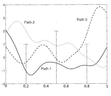
Figure 2: Cylinder sets.

Theorem 4.15.

Let $P_{n}$ be probability measures on $(\boldsymbol{C},\mathcal{C})$. If their finite-dimensional distributions converge weakly $P_{n}\pi^{-1}_{t_{1},\ldots,t_{k}}\Rightarrow\mu_{t_{1},\ldots,t_{k}}$, and if $P_{n}$ is tight, then

(a) there exists a probability measure $P$ on $(\boldsymbol{C},\mathcal{C})$ with $P\pi^{-1}_{t_{1},\ldots,t_{k}}=\mu_{t_{1},\ldots,t_{k}}$, and

(b) $P_{n}\Rightarrow P$.

Proof. Tightness implies relative compactness which in turn implies that each subsequence $(P_{n^{\prime}})\subset(P_{n})$ contains a further subsequence $(P_{n^{\prime\prime}})\subset(P_{n^{\prime}})$ converging weakly to some probability measure $P$. By the mapping theorem $P_{n^{\prime\prime}}\pi^{-1}_{t_{1},\ldots,t_{k}}\Rightarrow P\pi^{-1}_{t_{1},\ldots,t_{k}}$. Thus by hypothesis, $P\pi^{-1}_{t_{1},\ldots,t_{k}}=\mu_{t_{1},\ldots,t_{k}}$. Moreover, by Lemma 4.13, the limit $P$ must be the same for all converging subsequences, thus applying Theorem 3.8 we may conclude that $P_{n}\Rightarrow P$.

4.2 Wiener measure and Donsker’s theorem

Definition 4.16.

Let $\xi_{i}$ be a sequence of r.v. defined on the same probability space $(\Omega,\mathcal{F},\mathbb{P})$. Put $S_{n}=\xi_{1}+\ldots+\xi_{n}$ and let $X^{n}_{t}(\omega)$ as a function of $t$ be the element of $\boldsymbol{C}$ defined by linear interpolation between its values $X^{n}_{i/n}(\omega)={S_{i}(\omega)\over\sigma\sqrt{n}}$ at the points $t=i/n$.

Theorem 4.17.

Let $X^{n}=(X^{n}_{t}:0\leq t\leq 1)$ be defined by Definition 4.16 and let $P_{n}$ be the probability distribution of $X^{n}$. If $\xi_{i}$ are iid with zero mean and finite variance $\sigma^{2}$, then

(a) $P_{n}\pi^{-1}_{t_{1},\ldots,t_{k}}\Rightarrow\mu_{t_{1},\ldots,t_{k}}$, where $\mu_{t_{1},\ldots,t_{k}}$ are Gaussian distributions on $\boldsymbol{R}^{k}$ satisfying

$$\mu_{t_{1},\ldots,t_{k}}\big{\{}(x_{1},\ldots,x_{k}):x_{i}-x_{i-1}\leq\alpha_{i},i=1,\ldots,k\big{\}}=\prod_{i=1}^{k}\Phi\Big{(}{\alpha_{i}\over\sqrt{t_{i}-t_{i-1}}}\Big{)},\mbox{ where }x_{0}=0,$$

(b) the sequence $(P_{n})$ of probability measures on $(\boldsymbol{C},\mathcal{C})$ is tight.

Proof. The claim (a) follows from the classical CLT and independence of increments of $S_{n}$. For example, if $0\leq s\leq t\leq 1$, then

$$(X^{n}_{s},X^{n}_{t}-X^{n}_{s}) ={1\over\sigma\sqrt{n}}(S_{\lfloor ns\rfloor},S_{\lfloor nt\rfloor}-S_{\lfloor ns\rfloor})+\epsilon^{n}_{s,t},$$

$$\epsilon^{n}_{s,t} ={1\over\sigma\sqrt{n}}(\{ns\}\xi_{\lfloor ns\rfloor+1},\{nt\}\xi_{\lfloor nt\rfloor+1}-\{ns\}\xi_{\lfloor ns\rfloor+1}),$$

where $\{nt\}$ stands for the fractional part of $nt$. By the classical CLT and Theorem 2.7c, ${1\over\sigma\sqrt{n}}(S_{\lfloor ns\rfloor},S_{\lfloor nt\rfloor}-S_{\lfloor ns\rfloor})$ has $\mu_{s,t}$ as a limit distribution. Applying Corollary 1.24 to $\epsilon^{n}_{s,t}$, we derive $P_{n}\pi^{-1}_{s,t}\Rightarrow\mu_{s,t}$.

The proof of (b) is postponed until the next subsection.

Definition 4.18.

Wiener measure $\mathbb{W}$ is a probability measure on $\boldsymbol{C}$ with $\mathbb{W}\pi^{-1}_{t_{1},\ldots,t_{k}}=\mu_{t_{1},\ldots,t_{k}}$ given by the formula in Theorem 4.17 part (a). The standard Wiener process $W$ is the random element on $(\boldsymbol{C},\mathcal{C},\mathbb{W})$ defined by $W_{t}(x)=x(t)$.

The existence of $\mathbb{W}$ follows from Theorems 4.15 and 4.17.

Theorem 4.19.

Let $X^{n}=(X^{n}_{t}:0\leq t\leq 1)$ be defined by Definition 4.16. If $\xi_{i}$ are iid with zero mean and finite variance $\sigma^{2}$, then $X^{n}$ converges in distribution to the standard Wiener process.

Proof 1. This is a corollary of Theorems 4.15 and 4.17.

Proof 2. An alternative proof is based on Theorem 4.12. We have to verify that condition (i) of Theorem 4.12 holds under the assumptions of Theorem 4.17. To this end take $t_{j}=j\delta$, $j=0,\ldots,\delta^{-1}$ assuming $n\delta>1$. Then

$$\mathbb{P}(w(X^{n},\delta)\geq 3\epsilon) \leq\sum_{j=1}^{1/\delta}\mathbb{P}\Big{(}\sup_{t_{j-1}\leq s\leq t_{j}}|X^{n}_{s}-X^{n}_{t_{j-1}}|\geq\epsilon\Big{)}$$

$$=\sum_{j=1}^{1/\delta}\mathbb{P}\Big{(}\operatorname*{\vphantom{p}max}_{(j-1)n\delta\leq k\leq jn\delta}{|S_{k}-S_{(j-1)n\delta}|\over\sigma\sqrt{n}}\geq\epsilon\Big{)}=\sum_{j=1}^{1/\delta}\mathbb{P}\Big{(}\operatorname*{\vphantom{p}max}_{k\leq n\delta}|S_{k}|\geq\epsilon\sigma\sqrt{n}\Big{)}$$

$$=\delta^{-1}\mathbb{P}\Big{(}\operatorname*{\vphantom{p}max}_{k\leq n\delta}|S_{k}|\geq\epsilon\sigma\sqrt{n}\Big{)}\leq 3\delta^{-1}\operatorname*{\vphantom{p}max}_{k\leq n\delta}\mathbb{P}\Big{(}|S_{k}|\geq\epsilon\sigma\sqrt{n}/3\Big{)},$$

where the last is Etemadi’s inequality:

$$\mathbb{P}\Big{(}\operatorname*{\vphantom{p}max}_{k\leq n}|S_{k}|\geq\alpha\Big{)}\leq 3\operatorname*{\vphantom{p}max}_{k\leq n}\mathbb{P}\Big{(}|S_{k}|\geq\alpha/3\Big{)}.$$

Remark: compare this with Kolmogorov’s inequality $\mathbb{P}(\operatorname*{\vphantom{p}max}_{k\leq n}|S_{k}|\geq\alpha)\leq{n\sigma^{2}\over\alpha^{2}}$.

It suffices to check that assuming $\sigma=1$,

$$\operatorname*{\vphantom{p}lim}_{\lambda\to\infty}\limsup_{n\to\infty}\lambda^{2}\operatorname*{\vphantom{p}max}_{k\leq n}\mathbb{P}\Big{(}|S_{k}|\geq\epsilon\lambda\sqrt{n}\Big{)}=0.$$

Indeed, by the classical CLT,

$$\mathbb{P}(|S_{k}|\geq\epsilon\lambda\sqrt{k})<4(1-\Phi(\epsilon\lambda))\leq{6\over\epsilon^{4}\lambda^{4}}$$

for sufficiently large $k\geq k(\lambda\epsilon)$. It follows,

$$\limsup_{n\to\infty}\lambda^{2}\operatorname*{\vphantom{p}max}_{k(\lambda\epsilon)\leq k\leq n}\mathbb{P}\Big{(}|S_{k}|\geq\epsilon\lambda\sqrt{n}\Big{)}\leq\limsup_{n\to\infty}\lambda^{2}\operatorname*{\vphantom{p}max}_{k\geq k(\lambda\epsilon)}\mathbb{P}\Big{(}|S_{k}|\geq\epsilon\lambda\sqrt{k}\Big{)}\leq{6\over\epsilon^{4}\lambda^{2}}.$$

On the other hand, by Chebyshev’s inequality,

$$\limsup_{n\to\infty}\lambda^{2}\operatorname*{\vphantom{p}max}_{k\leq k(\lambda\epsilon)}\mathbb{P}\Big{(}|S_{k}|\geq\epsilon\lambda\sqrt{n}\Big{)}\leq\limsup_{n\to\infty}{\lambda^{2}k(\lambda\epsilon)\over\epsilon^{2}\lambda^{2}n}=0$$

finishing the proof of (i) of Theorem 4.12.

Example 4.20.

We show that $h(x)=\sup_{t}x(t)$ is a continuous mapping from $\boldsymbol{C}$ to $\boldsymbol{R}$. Indeed, if $h(x)\geq h(y)$, then there are $t_{i}$ such that

$$0\leq h(x)-h(y)=x(t_{1})-y(t_{2})\leq x(t_{1})-y(t_{1})\leq\|x-y\|.$$

Thus, we have $|h(x)-h(y)|\leq\rho(x,y)$ and continuity follows.

Example 4.21.

Turning to the symmetric simple random walk, put $M_{n}=\operatorname*{\vphantom{p}max}(S_{0},\ldots,S_{n})$. As we show later in Theorem 5.1, for any $b\geq 0$,

$$\mathbb{P}(M_{n}\leq b\sqrt{n})\to{2\over\sqrt{2\pi}}\int_{0}^{b}e^{-u^{2}/2}du.$$

From $h(X^{n})\Rightarrow h(W)$ with $h(x)=\sup_{t}x(t)$ we conclude that $\sup_{0\leq t\leq 1}W_{t}$ is distributed as $|W_{1}|$. The same limit holds for $M_{n}=\operatorname*{\vphantom{p}max}({S_{0}\over\sigma},{S_{1}-\mu\over\sigma}\ldots,{S_{n}-n\mu\over\sigma})$ for sums of iid r.v. with mean $\mu$ and standard deviation $\sigma$. For this reason the functional CLT is also called an invariance principle: the general limit can be computed via the simplest relevant case.

Exercise 4.22.

Check if the following functionals are continuous on $\boldsymbol{C}$:

$$\sup_{\{0\leq s,t\leq 1\}}|x(t)-x(s)|,\qquad\int_{0}^{1}x(t)dt.$$

4.3 Tightness in $\boldsymbol{C}$

Theorem 4.23.

The Arzela-Ascoli theorem. The set $A\subset\boldsymbol{C}$ is relatively compact if and only if

$$(i) \quad\sup_{x\in A}|x(0)|<\infty,$$

$$(ii) \quad\operatorname*{\vphantom{p}lim}_{\delta\to 0}\sup_{x\in A}w_{x}(\delta)=0.$$

Proof. Necessity. If the closure of $A$ is compact, then (i) obviously must hold. For a fixed $x$ the function $w_{x}(\delta)$ monotonely converges to zero as $\delta\downarrow 0$. Since for each $\delta$ the function $w_{x}(\delta)$ is continuous in $x$ this convergence is uniform over $x\in K$ for any compact $K$. It remains to see that taking $K$ to be the closure of $A$ we obtain (ii).

Sufficiency. Suppose now that (i) and (ii) hold. For a given $\epsilon>0$, choose $n$ large enough for $\sup_{x\in A}w_{x}(1/n)<\epsilon$. Since

$$|x(t)|\leq|x(0)|+\sum_{i=1}^{n}|x(ti/n)-x(t(i-1)/n)|\leq|x(0)|+n\sup_{x\in A}w_{x}(1/n),$$

we derive $\alpha:=\sup_{x\in A}\|x\|<\infty$. The idea is to use this and (ii) to prove that $A$ is totally bounded, since $\boldsymbol{C}$ is complete, it will follow that $A$ is relatively compact. In other words, we have to find a finite $B_{\epsilon}\subset\boldsymbol{C}$ forming a $2\epsilon$-net for $A$.

Let $-\alpha=\alpha_{0}<\alpha_{1}<\ldots<\alpha_{k}=\alpha$ be such that $\alpha_{j}-\alpha_{j-1}\leq\epsilon$. Then $B_{\epsilon}$ can be taken as a set of the continuous polygonal functions $y:[0,1]\to[-\alpha,\alpha]$ that linearly connect the pairs of points $({i-1\over n},\alpha_{j_{i-1}}),({i\over n},\alpha_{j_{i}})$. See Figure 3. Let $x\in A$. It remains to show that there is a $y\in B_{\epsilon}$ such that $\rho(x,y)\leq 2\epsilon$. Indeed, since $|x(i/n)|\leq\alpha$, there is a $y\in B_{\epsilon}$ such that $|x(i/n)-y(i/n)|<\epsilon$ for all $i=0,1,\ldots,n$. Both $y(i/n)$ and $y((i-1)/n)$ are within $2\epsilon$ of $x(t)$ for $t\in[(i-1)/n,i/n]$. Since $y(t)$ is a convex combination of $y(i/n)$ and $y((i-1)/n)$, it too is within $2\epsilon$ of $x(t)$. Thus $\rho(x,y)\leq 2\epsilon$ and $B_{\epsilon}$ is a $2\epsilon$-net for $A$.

Figure 3: The Arzela-Ascoli theorem: constructing a $2\epsilon$-net.

Exercise 4.24.

Draw a curve $x\in A$ (cf Figure 3) for which you can not find a $y\in B_{\epsilon}$ such that $\rho(x,y)\leq\epsilon$.

The next theorem explains the nature of condition (i) in Theorem 4.12.

Theorem 4.25.

Let $P_{n}$ be probability measures on $(\boldsymbol{C},\mathcal{C})$. The sequence $(P_{n})$ is tight if and only if the following two conditions hold:

$$(i) \quad\operatorname*{\vphantom{p}lim}_{a\to\infty}\limsup_{n\to\infty}P_{n}(x:|x(0)|\geq a)=0,$$

$$(ii) \quad\operatorname*{\vphantom{p}lim}_{\delta\to 0}\limsup_{n\to\infty}P_{n}(x:w_{x}(\delta)\geq\epsilon)=0,\mbox{ for each positive }\epsilon.$$

Proof. Suppose $(P_{n})$ is tight. Given a positive $\eta$, choose a compact $K$ such that $P_{n}(K)>1-\eta$ for all $n$. By the Arzela-Ascoli theorem we have $K\subset(x:|x(0)|\leq a)$ for large enough $a$ and $K\subset(x:w_{x}(\delta)\leq\epsilon)$ for small enough $\delta$. Hence the necessity.

According to condition (i), for each positive $\eta$, there exist large $a_{\eta}$ and $n_{\eta}$ such that

$$P_{n}(x:|x(0)|\geq a_{\eta})\leq\eta,\quad n\geq n_{\eta},$$

and condition (ii) implies that for each positive $\epsilon$ and $\eta$, there exist a small $\delta_{\epsilon,\eta}$ and a large $n_{\epsilon,\eta}$ such that

$$P_{n}(x:w_{x}(\delta_{\epsilon,\eta})\geq\epsilon)\leq\eta,\quad n\geq n_{\epsilon,\eta},$$

Due to Lemma 3.2 for any finite $k$ the measure $P_{k}$ is tight, and so by the necessity there is a $a_{k,\eta}$ such that $P_{k}(x:|x(0)|\geq a_{k,\eta})\leq\eta$, and there is a $\delta_{k,\epsilon,\eta}$ such that $P_{k}(x:w_{x}(\delta_{k,\epsilon,\eta})\geq\epsilon)\leq\eta$.

Thus in proving sufficiency, we may put $n_{\eta}=n_{\epsilon,\eta}=1$ in the above two conditions. Fix an arbitrary small positive $\eta$. Given the two improved conditions, we have $P_{n}(B)\geq 1-\eta$ and $P_{n}(B_{k})\geq 1-2^{-k}\eta$ with $B=(x:|x(0)|<a_{\eta})$ and $B_{k}=(x:w_{x}(\delta_{1/k,2^{-k}\eta})<1/k)$. If $K$ is the closure of intersection of $B\cap B_{1}\cap B_{2}\cap\ldots$, then $P_{n}(K)\geq 1-2\eta$. To finish the proof observe that $K$ is compact by the Arzela-Ascoli theorem.

Example 4.26.

Consider the Dirac probability measure $P_{n}$ concentrated on the point $z_{n}\in\boldsymbol{C}$ from Example 4.3. Referring to Theorem 4.25 verify that the sequence $(P_{n})$ is not tight.

Proof of Theorem 4.17 part b. The stated tightness follows from Theorem 4.25. Indeed, condition (i) in Theorem 4.25 is trivially fulfilled as $X^{n}_{0}\equiv 0$. Furthermore, condition (i) of Theorem 4.12 (established in the proof 2 of Theorem 4.19) translates into (ii) in Theorem 4.25.

5 Applications of the functional CLT

5.1 The minimum and maximum of the Brownian path

Theorem 5.1.

Consider the standard Wiener process $W=(W_{t},0\leq t\leq 1)$ and let

$$m=\operatorname*{\vphantom{p}inf}_{0\leq t\leq 1}W_{t},\qquad M=\sup_{0\leq t\leq 1}W_{t}.$$

If $a\leq 0\leq b$ and $a\leq a^{\prime}<b^{\prime}\leq b$, then

$$\mathbb{P}( a<m\leq M<b;\ a^{\prime}<W_{1}<b^{\prime})$$

$$=\sum_{k=-\infty}^{\infty}\Big{(}\Phi(2k(b-a)+b^{\prime})-\Phi(2k(b-a)+a^{\prime})\Big{)}$$

$$\qquad-\sum_{k=-\infty}^{\infty}\Big{(}\Phi(2k(b-a)+2b-a^{\prime})-\Phi(2k(b-a)+2b-b^{\prime})\Big{)},$$

so that with $a^{\prime}=a$ and $b^{\prime}=b$ we get

$$\mathbb{P}( a<m\leq M<b)=\sum_{k=-\infty}^{\infty}(-1)^{k}\Big{(}\Phi(k(b-a)+b)-\Phi(k(b-a)+a)\Big{)}.$$

Proof. Let $S_{n}$ be the symmetric simple random walk and put $m_{n}=\min(S_{0},\ldots,S_{n})$, $M_{n}=\operatorname*{\vphantom{p}max}(S_{0},\ldots,S_{n})$. Since the mapping of $\boldsymbol{C}$ into $\boldsymbol{R}^{3}$ defined by

$$x\to\big{(}\operatorname*{\vphantom{p}inf}_{t}x(t),\sup_{t}x(t),x(1)\big{)}$$

is continuous, the functional CLT entails $n^{-1/2}(m_{n},M_{n},S_{n})\Rightarrow(m,M,W_{1})$. The theorem’s main statement will be obtained in two steps.

Step 1: show that for integers satisfying $i<0<j$ and $i\leq i^{\prime}<j^{\prime}\leq j$,

$$\mathbb{P}(i<m_{n}\leq M_{n}<j;\ i^{\prime}<S_{n}<j^{\prime})$$

$$=\sum_{k=-\infty}^{\infty}\mathbb{P}(2k(j-i)+i^{\prime}<S_{n}<2k(j-i)+j^{\prime})$$

$$\quad-\sum_{k=-\infty}^{\infty}\mathbb{P}(2k(j-i)+2j-j^{\prime}<S_{n}<2k(j-i)+2j-i^{\prime}).$$

In other words, we have to show that for $i<0<j$, $i<l<j$

$$\mathbb{P}(i<m_{n}\leq M_{n}<j;\ S_{n}=l) =\sum_{k=-\infty}^{\infty}\mathbb{P}(S_{n}=2k(j-i)+l)$$

$$\qquad-\sum_{k=-\infty}^{\infty}\mathbb{P}(S_{n}=2k(j-i)+2j-l).\qquad\qquad(*)$$

Observe that here both series are just finite sums as $|S_{n}|\leq n$.

Equality $(*)$ is proved by induction on $n$. For $n=1$, if $j>1$, then

$$\mathbb{P}(i<m_{1} \leq M_{1}<j;\ S_{1}=1)=\mathbb{P}(S_{1}=1)$$

$$=\sum_{k=-\infty}^{\infty}\mathbb{P}(S_{1}=2k(j-i)+1)-\sum_{k=-\infty}^{\infty}\mathbb{P}(S_{1}=2k(j-i)+2j-1),$$

and if $i<-1$, then

$$\mathbb{P}(i<m_{1} \leq M_{1}<j;\ S_{1}=-1)=\mathbb{P}(S_{1}=-1)$$

$$=\sum_{k=-\infty}^{\infty}\mathbb{P}(S_{1}=2k(j-i)-1)-\sum_{k=-\infty}^{\infty}\mathbb{P}(S_{1}=2k(j-i)+2j+1).$$

Assume as induction hypothesis that the statement holds for $(n-1,i,j,l)$ with all relevant triplets $(i,j,l)$. Conditioning on the first step of the random walk, we get

$$\mathbb{P}(i<m_{n}\leq M_{n}<j;\ S_{n}=l) ={1\over 2}\cdot\mathbb{P}(i-1<m_{n-1}\leq M_{n-1}<j-1;\ S_{n-1}=l-1)$$

$$+{1\over 2}\cdot\mathbb{P}(i+1<m_{n-1}\leq M_{n-1}<j+1;\ S_{n-1}=l+1),$$

which together with the induction hypothesis yields the stated equality $(*)$

$$2\mathbb{P}( i<m_{n}\leq M_{n}<j;\ S_{n}=l)$$

$$=\sum_{k=-\infty}^{\infty}\Big{(}\mathbb{P}(S_{n-1}=2k(j-i)+l-1)+\mathbb{P}(S_{n-1}=2k(j-i)+l+1)\Big{)}$$

$$\quad-\sum_{k=-\infty}^{\infty}\Big{(}\mathbb{P}(S_{n-1}=2k(j-i)+2j-l+1)+\mathbb{P}(S_{n-1}=2k(j-i)+2j-l-1)\Big{)}$$

$$=2\sum_{k=-\infty}^{\infty}\mathbb{P}(S_{n}=2k(j-i)+l)-2\sum_{k=-\infty}^{\infty}\mathbb{P}(S_{n}=2k(j-i)+2j-l).$$

Step 2: show that for $c>0$ and $a<b$,

$$\sum_{k=-\infty}^{\infty}\mathbb{P}\Big{(}2k\lfloor c\sqrt{n}\rfloor+\lfloor a\sqrt{n}\rfloor< S_{n}<2k\lfloor c\sqrt{n}\rfloor+\lfloor b\sqrt{n}\rfloor\Big{)}$$

$$\to\sum_{k=-\infty}^{\infty}\Big{(}\Phi(2kc+b)-\Phi(2kc+a)\Big{)},\quad n\to\infty.$$

This is obtained using the CLT. The interchange of the limit with the summation over $k$ follows from

$$\operatorname*{\vphantom{p}lim}_{k_{0}\to\infty}\sum_{|k|>k_{0}}\mathbb{P}\Big{(}2k\lfloor c\sqrt{n}\rfloor+\lfloor a\sqrt{n}\rfloor<S_{n}<2k\lfloor c\sqrt{n}\rfloor+\lfloor b\sqrt{n}\rfloor\Big{)}=0,$$

which in turn can be justified by the following series form of Scheffe’s theorem. If $\sum_{k}s_{kn}=\sum_{k}s_{k}=1$, the terms being nonnegative, and if $s_{kn}\to s_{k}$ for each $k$, then $\sum_{k}r_{k}s_{kn}\to\sum_{k}r_{k}s_{k}$ provided $r_{k}$ is bounded. To apply this in our case we should take

$$s_{kn}=\mathbb{P}\Big{(}2k\lfloor\sqrt{n}\rfloor-\lfloor\sqrt{n}\rfloor<S_{n}\leq 2k\lfloor\sqrt{n}\rfloor+\lfloor\sqrt{n}\rfloor\Big{)},\quad s_{k}=\Phi(2k+1)-\Phi(2k-1).$$

Corollary 5.2.

Consider the standard Wiener process $W$. If $a\leq 0\leq b$, then

$$\mathbb{P}(\sup_{0\leq t\leq 1}W_{t}<b) =2\Phi(b)-1,$$

$$\mathbb{P}(\operatorname*{\vphantom{p}inf}_{0\leq t\leq 1}W_{t}>a) =1-2\Phi(a),$$

$$\mathbb{P}(\sup_{0\leq t\leq 1}|W_{t}|<b) =2\sum_{k=-\infty}^{\infty}\Big{\{}\Phi((4k+1)b)-\Phi((4k-1)b)\Big{\}}.$$

5.2 The arcsine law

Lemma 5.3.

For $x\in\boldsymbol{C}$ and a Borel measurable, bounded $v:\boldsymbol{R}\to\boldsymbol{R}$, put $h(x)=\int_{0}^{1}v(x(t))dt$. If $v$ is continuous except on a set $D_{v}$ with $\lambda(D_{v})=0$, where $\lambda$ is the Lebesgue measure, then $h$ is $\mathcal{C}$-measurable and is continuous except on a set of Wiener measure 0.

Proof. Since both mappings $x\to x(t)$ and $t\to x(t)$ are continuous, the mapping $(x,t)\to x(t)$ is continuous in the product topology and therefore Borel measurable. It follows that the mapping $\psi(x,t)=v(x(t))$ is also measurable. Since $\psi$ is bounded, $h(x)=\int_{0}^{1}\psi(x,t)dt$ is $\mathcal{C}$-measurable, see Fubini’s theorem.

Let $E=\{(x,t):x(t)\in D_{v}\}$. If $\mathbb{W}$ is Wiener measure on $(\boldsymbol{C},\mathcal{C})$, then by the hypothesis $\lambda(D_{v})=0$,

$$\mathbb{W}\{x:(x,t)\in E\}=\mathbb{W}\{x:x(t)\in D_{v}\}=0\mbox{ for each }t\in[0,1].$$

It follows by Fubini’s theorem applied to the measure $\mathbb{W}\times\lambda$ on $\boldsymbol{C}\times[0,1]$ that $\lambda\{t:(x,t)\in E\}=0$ for all $x$ outside a set $A_{v}\in\mathcal{C}$ satisfying $\mathbb{W}(A_{v})=0$. Suppose that $\|x_{n}-x\|\to 0$. If $x\notin A_{v}$, then $x(t)\notin D_{v}$ for almost all $t$ and hence $v(x_{n}(t))\to v(x(t))$ for almost all $t$. It follows by the bounded convergence theorem that

$$\mbox{if }x\notin A_{v}\mbox{ and }\|x_{n}-x\|\to 0,\quad\mbox{ then }\int_{0}^{1}v(x_{n}(t))dt\to\int_{0}^{1}v(x(t))dt.$$

Exercise 5.4.

Let $W$ be a standard Wiener process and $t_{0}\in(0,1)$. Put $W^{\prime}_{s}={W_{t}-W_{t_{0}}\over\sqrt{1-t_{0}}}$ for $s={t-t_{0}\over 1-t_{0}}$, $t\in[t_{0},1]$. Using the Donsker invariance principle show that $(W^{\prime}_{s},0\leq s\leq 1)$ is also distributed as a standard Wiener process.

Lemma 5.5.

Each of the following three mappings $h_{i}:\boldsymbol{C}\to\boldsymbol{R}$

$$h_{1}(x) =\sup\{t:x(t)=0,t\in[0,1]\},$$

$$h_{2}(x) =\lambda\{t:x(t)>0,t\in[0,1]\},$$

$$h_{3}(x) =\lambda\{t:x(t)>0,t\in[0,h_{1}(x)]\}$$

is $\mathcal{C}$-measurable and continuous except on a set of Wiener measure 0.

Proof. Using the previous lemma with $v(z)=1_{\{z\in(0,\infty)\}}$ we obtain the assertion for $h_{2}$.

Turning to $h_{1}$, observe that

$$\{x:h_{1}(x)<\alpha\}=\{x:x(t)>0,t\in[\alpha,1]\}\cup\{x:x(t)<0,t\in[\alpha,1]\}$$

is open and hence $h_{1}$ is measurable. If $h_{1}$ is discontinuous at $x$, then there exist $0<t_{0}<t_{1}<1$ such that $x(t_{1})=0$ and

$$\mbox{either }\quad x(t)>0\mbox{ for all }t\in[t_{0},1]\setminus\{t_{1}\}\quad\mbox{ or }\quad x(t)<0\mbox{ for all }t\in[t_{0},1]\setminus\{t_{1}\}.$$

That $h_{1}$ is continuous except on a set of Wiener measure 0 will therefore follow if we show that, for each $t_{0}$, the random variables

$$M_{0}=\sup\{W_{t},t\in[t_{0},1]\}\quad\mbox{ and }\quad\operatorname*{\vphantom{p}inf}\{W_{t},t\in[t_{0},1]\}$$

have continuous distributions. By the last exercise and Theorem 5.1, $M^{\prime}=M_{0}-W_{t_{0}}$ has a continuous distribution. Because $M^{\prime}$ and $W_{t_{0}}$ are independent, we conclude that their sum also has a continuous distribution. The infimum is treated the same way.

Finally, for $h_{3}$, use the representation

$$h_{3}(x)=\psi(x,h_{1}(x)),\quad\mbox{ where }\psi(x,t)=\int_{0}^{t}v(x(u))du\quad\mbox{ with }v(z)=1_{\{z\in(0,\infty)\}}.$$

Theorem 5.6.

Consider the standard Wiener process $W$ and let

$T=h_{1}(W)$ be the time at which $W$ last passes through 0,

$U=h_{2}(W)$ be the total amount of time $W$ spends above 0, and

$V=h_{3}(W)$ be the total amount of time $W$ spends above 0 in the interval $[0,T]$.

so that

$$U=V+(1-T)1_{\{W_{1}\geq 0\}}.$$

Then the triplet $(T,V,W_{1})$ has the joint density

$$f(t,v,z)=1_{\{0<v<t<1\}}g(t,z),\quad g(t,z)={1\over 2\pi}{|z|\over t^{3/2}(1-t)^{3/2}}e^{-{z^{2}\over 2(1-t)}}.$$

In particular, the conditional distribution of $V$ given $(T,W_{1})$ is uniform on $[0,T]$, and

$$\mathbb{P}(T\leq t)=\mathbb{P}(U\leq t)={2\over\pi}\arcsin(\sqrt{t}),\quad 0<t<1.$$

Proof. The main idea is to apply the invariance principle via the symmetric simple random walk $S_{n}$. We will use three properties of $S_{n}$ and its path functionals $(T_{n},U_{n},V_{n})$. First, we need the local limit theorem for $p_{n}(i)=\mathbb{P}(S_{n}=i)$ similar to that of Example 1.29:

$$\mbox{if }{i\over\sqrt{n}}\to z,\mbox{ with }n-i\mbox{ being even},\mbox{ then }{\sqrt{n}\over 2}p_{n}(i)\to{1\over\sqrt{2\pi}}e^{-z^{2}/2}.$$

Second, we need the fact that

$$\mathbb{P}(S_{1}\geq 1,\ldots,S_{n-1}\geq 1,S_{n}=i)={i\over n}p_{n}(i),\quad i\geq 1.$$

The third fact we need is that if $S_{2n}=0$, then $U_{2n}=V_{2n}$ and

$$\mathbb{P}(V_{2n}=2j|S_{2n}=0)={1\over n+1},\quad j=0,1,\ldots,n.$$

Using these three facts we obtain that for $0\leq 2j\leq 2k<n$ and $i\geq 1$,

$$\mathbb{P}(T_{n}=2k, V_{2n}=2j,S_{n}=i)$$

$$=\mathbb{P}(S_{2k}=0,V_{2n}=2j,S_{2k+1}\geq 1,\ldots,S_{n-1}\geq 1,S_{n}=i)$$

$$=\mathbb{P}(S_{2k}=0)\mathbb{P}(V_{2k}=2j|S_{2k}=0)\mathbb{P}(S_{2k+1}\geq 1,\ldots,S_{n-1}\geq 1,S_{n}=i|S_{2k}=0)$$

$$=p_{2k}(0){1\over k+1}{i\over n-2k}p_{n-2k}(i).$$

We apply Theorem 1.28 to the three-dimensional lattice of points $({2k\over n},{2j\over n},{i\over\sqrt{n}})$ for which $i\equiv n\mbox{ (mod 2)}$. The volume of the corresponding cell is ${2\over n}\cdot{2\over n}\cdot{2\over\sqrt{n}}=8n^{-5/2}$. If

$${2k\over n}\to t,\quad{2j\over n}\to v,\quad{i\over\sqrt{n}}\to z,\quad 0<v<t<1,\quad z>0,$$

then

$${n^{5/2}\over 8}\mathbb{P}(T_{n}=2k, V_{2n}=2j,S_{n}=i)$$

$$={\sqrt{n}\over\sqrt{2k}}{\sqrt{2k}\over 2}p_{2k}(0){n\over 2(k+1)}{i\over\sqrt{n}}{n\over n-2k}{\sqrt{n}\over\sqrt{n-2k}}{\sqrt{n-2k}\over 2}p_{n-2k}(i)$$

$$\to{1\over\sqrt{2\pi}}{1\over t^{3/2}}z{1\over(1-t)^{3/2}}{1\over\sqrt{2\pi}}e^{-{z^{2}\over 2(1-t)}}=g(t,z).$$

The same result holds for negative $z$ by symmetry.

The joint density of $(T,W_{1})$ is $tg(t,z)1_{\{0<t<1\}}$, hence the marginal density for $T$ equals

$$f_{T}(t) =\int_{-\infty}^{\infty}tg(t,z)dz=\int_{0}^{\infty}e^{-{z^{2}\over 2(1-t)}}{zdz\over\pi(1-t)^{3/2}t^{1/2}}={1\over\pi(1-t)^{1/2}t^{1/2}}$$

implying

$$\mathbb{P}(T\leq t)={2\over\pi}\arcsin(\sqrt{t}),\quad 0<t<1.$$

Notice also that

$$G(u) :=\int_{-\infty}^{\infty}\int_{u}^{1}g(t,z)dtdz=\int_{u}^{1}\int_{0}^{\infty}e^{-{z^{2}\over 2(1-t)}}{zdz\over\pi(1-t)^{3/2}t^{3/2}}dt$$

$$=\int_{u}^{1}{dt\over\pi(1-t)^{1/2}t^{3/2}}=-{2\over\pi}\int_{u}^{1}{dt^{-1/2}\over\sqrt{1-t}}={2\over\pi}\int_{1}^{u^{-1/2}}{ydy\over\sqrt{y^{2}-1}}={2\over\pi}\sqrt{u^{-1}-1}.$$

If $(T,W_{1})=(t,z)$, then $U$ is distributed uniformly over $[1-t,1]$ for $z\geq 0$, and uniformly over $[0,t]$ for $z<0$:

$$\mathbb{P}(U\leq u|T=t,W_{1}=z) ={u-1+t\over t}1_{\{u\in[1-t,1],z\geq 0\}}+{u\over t}1_{\{u\in[0,t],z<0\}}+1_{\{u\in(t,1],z<0\}}.$$

Thus the marginal distribution function of $U$ equals

$$\mathbb{P}(U\leq u) =\mathbb{E}\Big{(}{u-1+T\over T}1_{\{u\in[1-T,1],W_{1}\geq 0\}}+{u\over T}1_{\{u\in[0,T],W_{1}<0\}}+1_{\{u\in(T,1],W_{1}<0\}}\Big{)}$$

$$=\int_{0}^{\infty}\int_{1-u}^{1}(u-1+t)g(t,z)dtdz+\int_{-\infty}^{0}\int_{u}^{1}ug(t,z)dtdz+\int_{-\infty}^{0}\int_{0}^{u}tg(t,z)dtdz$$

$$={1\over 2}\int_{1-u}^{1}f_{T}(t)dt+{u-1\over 2}G(1-u)+{u\over 2}G(u)+{1\over 2}\int_{0}^{u}f_{T}(t)dt$$

$$={1\over 2}\mathbb{P}(T>1-u)+{1\over 2}\mathbb{P}(T\leq u)={2\over\pi}\arcsin(\sqrt{u}).$$

5.3 The Brownian bridge

Definition 5.7.

The transformed standard Wiener process $W^{\circ}_{t}=W_{t}-tW_{1}$, $t\in[0,1]$, is called the standard Brownian bridge.

Exercise 5.8.

Show that the standard Brownian bridge $W^{\circ}$ is a Gaussian process with zero mean and covariance $\mathbb{E}(W^{\circ}_{s}W^{\circ}_{t})=s(1-t)$ for $s\leq t$.

Example 5.9.

Define $h:\boldsymbol{C}\to\boldsymbol{C}$ by $h(x(t))=x(t)-tx(1)$. This is a continuous mapping since $\rho(h(x),h(y))\leq 2\rho(x,y)$, and $h(X^{n})\Rightarrow W^{\circ}$ by Theorem 4.19.

Theorem 5.10.

Let $P_{\epsilon}$ be the probability measure on $(\boldsymbol{C},\mathcal{C})$ defined by

$$P_{\epsilon}(A)=\mathbb{P}(W\in A|0\leq W_{1}\leq\epsilon),\quad A\in\mathcal{C}.$$

Then $P_{\epsilon}\Rightarrow\mathbb{W}^{\circ}$ as $\epsilon\to 0$, where $\mathbb{W}^{\circ}$ is the distribution of the Brownian bridge $W^{\circ}$.

Proof. We will prove that for every closed $F\in\mathcal{C}$

$$\limsup_{\epsilon\to 0}\mathbb{P}(W\in F|0\leq W_{1}\leq\epsilon)\leq\mathbb{P}(W^{\circ}\in F).$$

Using $W^{\circ}_{t}=W_{t}-tW_{1}$ we get $\mathbb{E}(W^{\circ}_{t}W_{1})=0$ for all $t$. From the normality we conclude that $W_{1}$ is independent of each $(W^{\circ}_{t_{1}},\ldots,W^{\circ}_{t_{k}})$. Therefore,

$$\mathbb{P}(W^{\circ}\in A,W_{1}\in B)=\mathbb{P}(W^{\circ}\in A)\mathbb{P}(W_{1}\in B),\quad A\in\mathcal{C}_{f},B\in\mathcal{R},$$

and since $\mathcal{C}_{f}$, the collection of finite-dimensional sets, see the proof of Lemma 4.13, is a separating class, it follows

$$\mathbb{P}(W^{\circ}\in A|0\leq W_{1}\leq\epsilon)=\mathbb{P}(W^{\circ}\in A),\quad A\in\mathcal{C},\epsilon>0.$$

Observe that $\rho(W,W^{\circ})=|W_{1}|$. Thus,

$$\{|W_{1}|\leq\delta\}\cap\{W\in F\}\subset\{W^{\circ}\in F_{\delta}\},\quad\mbox{where }F_{\delta}=\{x:\rho(x,F)\leq\delta\}.$$

Therefore, if $\epsilon<\delta$

$$\mathbb{P}(W\in F|0\leq W_{1}\leq\epsilon)\leq\mathbb{P}(W^{\circ}\in F_{\delta}|0\leq W_{1}\leq\epsilon)=\mathbb{P}(W^{\circ}\in F_{\delta}),$$

leading to the required result

$$\limsup_{\epsilon\to 0}\mathbb{P}(W\in F|0\leq W_{1}\leq\epsilon)\leq\limsup_{\delta\to 0}\mathbb{P}(W^{\circ}\in F_{\delta})=\mathbb{P}(W^{\circ}\in F).$$

Theorem 5.11.

Distribution functions for several functionals of the Brownian bridge:

$$\mathbb{P}\big{(}a<\operatorname*{\vphantom{p}inf}_{t}W^{\circ}_{t}\leq\sup_{t}W^{\circ}_{t}\leq b\big{)} =\sum_{k=-\infty}^{\infty}\Big{(}e^{-2k^{2}(b-a)^{2}}-e^{-2(b+k(b-a))^{2}}\Big{)},\quad a<0<b,$$

$$\mathbb{P}\big{(}\sup_{t}|W^{\circ}_{t}|\leq b\big{)} =1+2\sum_{k=1}^{\infty}(-1)^{k}e^{-2k^{2}b^{2}},\quad b>0,$$

$$\mathbb{P}\big{(}\sup_{t}W^{\circ}_{t}\leq b\big{)} =\mathbb{P}\big{(}\operatorname*{\vphantom{p}inf}_{t}W^{\circ}_{t}>-b\big{)}=1-e^{-2b^{2}},\quad b>0,$$

$$\mathbb{P}\big{(}h_{2}(W^{\circ})\leq u\big{)} =u,\quad u\in[0,1].$$

Proof. The main idea of the proof is the following. Suppose that $h:\boldsymbol{C}\to\boldsymbol{R}^{k}$ is a measurable mapping and that the set $D_{h}$ of its discontinuities satisfies $\mathbb{W}^{\circ}(D_{h})=0$. It follows by Theorem 5.10 and the mapping theorem that

$$\mathbb{P}(h(W^{\circ})\leq\alpha)=\operatorname*{\vphantom{p}lim}_{\epsilon\to 0}\mathbb{P}(h(W)\leq\alpha|0\leq W_{1}\leq\epsilon).$$

Using either this or alternatively,

$$\mathbb{P}(h(W^{\circ})\leq\alpha)=\operatorname*{\vphantom{p}lim}_{\epsilon\to 0}\mathbb{P}(h(W)\leq\alpha|-\epsilon\leq W_{1}\leq 0)$$

one can find explicit forms for distributions connected with $W^{\circ}$.

Turning to Theorem 5.1 with $a<0<b$ and $a^{\prime}=0,b^{\prime}=\epsilon$ we get

$$\mathbb{P}(a<m\leq M<b; \ 0<W_{1}<\epsilon)$$

$$=\sum_{k=-\infty}^{\infty}\Big{(}\Phi(2k(b-a)+\epsilon)-\Phi(2k(b-a))\Big{)}$$

$$\qquad-\sum_{k=-\infty}^{\infty}\Big{(}\Phi(2k(b-a)+2b)-\Phi(2k(b-a)+2b-\epsilon)\Big{)}.$$

This implies the first statement as

$${\Phi(z+\epsilon)-\Phi(z)\over\epsilon}\to{e^{-z^{2}/2}\over\sqrt{2\pi}}.$$

As for the last statement, we need to show, in terms of $U=h_{2}(W)$, that

$$\operatorname*{\vphantom{p}lim}_{\epsilon\to 0}\mathbb{P}(U\leq u|-\epsilon\leq W_{1}\leq 0)=u,$$

or, in terms of $V=h_{3}(W)$, that

$$\operatorname*{\vphantom{p}lim}_{\epsilon\to 0}\mathbb{P}(V\leq u|-\epsilon\leq W_{1}\leq 0)=u.$$

Recall that the distribution of $V$ for given $T$ and $W_{1}$ is uniform on $(0,T)$, in other words, $L=V/T$ is uniformly distributed on $(0,1)$ and is independent of $(T,W_{1})$. Thus,

$$\mathbb{P}(V\leq u|-\epsilon\leq W_{1}\leq 0) =\mathbb{P}(TL\leq u|-\epsilon\leq W_{1}\leq 0)$$

$$=\int_{0}^{1}\mathbb{P}(T\leq u/s|-\epsilon\leq W_{1}\leq 0)ds$$

$$=u+\int_{u}^{1}\mathbb{P}(T\leq u/s|-\epsilon\leq W_{1}\leq 0)ds.$$

It remains to see that

$$\int_{u}^{1}\mathbb{P}(T\leq u/s |-\epsilon\leq W_{1}\leq 0)ds={1\over\Phi(\epsilon)-\Phi(0)}\int_{u}^{1}\mathbb{P}(T\leq u/s;-\epsilon\leq W_{1}\leq 0)ds$$

$$\leq c\epsilon^{-1}\int_{u}^{1}\mathbb{P}(T\leq r;-\epsilon\leq W_{1}\leq 0){dr\over r^{2}}\leq c\epsilon^{-1}u^{-2}\int_{u}^{1}\int_{0}^{r}\int_{0}^{\epsilon}tg(t,z)dzdtdr$$

$$\leq c_{1}\epsilon u^{-2}\int_{0}^{1}{dt\over t^{1/2}(1-t)^{1/2}}\to 0,\quad\epsilon\to 0.$$

6 The space $\boldsymbol{D}=\boldsymbol{D}[0,1]$

6.1 Cadlag functions

Definition 6.1.

Let $\boldsymbol{D}=\boldsymbol{D}[0,1]$ be the space of functions $x:[0,1]\to\boldsymbol{R}$ that are right continuous and have left-hand limits.

Exercise 6.2.

If $x_{n}\in\boldsymbol{D}$ and $\|x_{n}-x\|\to 0$, then $x\in\boldsymbol{D}$.

For $x\in\boldsymbol{D}$ and $T\subset[0,1]$ we will use notation

$$w_{x}(T)=w(x,T)=\sup_{s,t\in T}|x(t)-x(s)|,$$

and write $w_{x}[t,t+\delta]$ instead of $w_{x}([t,t+\delta])$. This should not be confused with the earlier defined modulus of continuity

$$w_{x}(\delta)=w(x,\delta)=\sup_{0\leq t\leq 1-\delta}w_{x}[t,t+\delta],$$

Clearly, if $T_{1}\subset T_{2}$, then $w_{x}(T_{1})\leq w_{x}(T_{2})$. Hence $w_{x}(\delta)$ is monotone over $\delta$.

Example 6.3.

Consider $x_{n}(t)=$ the fractional part of $nt$. It has regular downward jumps of size $1$. For example, $x_{1}(t)=t$ for $t\in[0,1)$, and $x_{1}(1)=0$. Another example: $x_{2}(t)=2t$ for $t\in[0,1/2)$, $x_{2}(t)=2t-1$ for $t\in[1/2,1)$, and $x_{2}(1)=0$. Placing an interval $[t,t+\delta]$ around a jump, we find $w_{x_{n}}(\delta)\equiv 1$.

Lemma 6.4.

Consider an arbitrary $x\in\boldsymbol{D}$. For each $\epsilon>0$, there exist points $0=t_{0}<t_{1}<\ldots<t_{v}=1$ such that

$$w_{x}[t_{i-1},t_{i})<\epsilon,\quad i=1,2,\ldots,v.$$

It follows that $x$ is bounded, and that $x$ can be uniformly approximated by simple functions constant over intervals, so that it is Borel measurable. It follows also that $x$ has at most countably many jumps.

Proof. To prove the first statement, let $t^{\circ}=t^{\circ}(\epsilon)$ be the supremum of those $t\in[0,1]$ for which $[0,t)$ can be decomposed into finitely many subintervals satisfying $w_{x}[t_{i-1},t_{i})<\epsilon$. We show in three steps that $t^{\circ}=1$.

Step 1. Since $x(0)=x(0+)$, we have $w_{x}[0,\eta_{0})<\epsilon$ for some small positive $\eta_{0}$. Thus $t^{\circ}>0$.

Step 2. Since $x(t^{\circ}-)$ exists, we have $w_{x}[t^{\circ}-\eta_{1},t^{\circ})<\epsilon$ for some small positive $\eta_{1}$, which implies that the interval $[0,t^{\circ})$ can itself be so decomposed.

Step 3. Suppose $t^{\circ}=\tau$, where $\tau<1$. From $x(\tau)=x(\tau+)$ using the argument of the step 1, we see that according to the definition of $t^{\circ}$ we should have $t^{\circ}>\tau$.

The last statement of the lemma follows from the fact that for any natural $n$, there exist at most finitely many points $t$ at which $|x(t)-x(t-)|\geq n^{-1}$.

Exercise 6.5.

Find a bounded function $x\notin\boldsymbol{D}$ with the following property: for any set $0=t_{0}<t_{1}<\ldots<t_{v}=1$ there exists an $i$ such that $w_{x}[t_{i-1},t_{i})\geq 1$.

Definition 6.6.

Let $\delta\in(0,1)$. A set $0=t_{0}<t_{1}<\ldots<t_{v}=1$ is called $\delta$-sparse if $t_{i}-t_{i-1}>\delta$ for $i=1,\ldots,v$. Define an analog of the modulus of continuity $w_{x}(\delta)$ by

$$w^{\prime}_{x}(\delta) =w^{\prime}(x,\delta)=\operatorname*{\vphantom{p}inf}_{\{t_{i}\}}\operatorname*{\vphantom{p}max}_{1\leq i\leq v}w_{x}[t_{i-1},t_{i}),$$

where the infimum extends over all $\delta$-sparse sets $\{t_{i}\}$. The function $w_{x}^{\prime}(\delta)$ is called a cadlag modulus of $x$.

Exercise 6.7.

Using Lemma 6.4 show that a function $x:[0,1]\to\boldsymbol{R}$ belongs to $\boldsymbol{D}$ if and only if $w_{x}^{\prime}(\delta)\to 0$.

Exercise 6.8.

Compute $w^{\prime}_{x}(\delta)$ for $x=1_{[0,a)}$.

Lemma 6.9.

For any $x$, $w^{\prime}_{x}(\delta)$ is non-decreasing over $\delta$, and $w_{x}^{\prime}(\delta)\leq w_{x}(2\delta)$. Moreover, for any $x\in\boldsymbol{D}$,

$$j_{x}\leq w_{x}(\delta)\leq 2w_{x}^{\prime}(\delta)+j_{x},\quad j_{x}=\sup_{0<t\leq 1}|x(t)-x(t-)|.$$

Proof. Taking a $\delta$-sparse set with $t_{i}-t_{i-1}\leq 2\delta$ we get $w_{x}^{\prime}(\delta)\leq w_{x}(2\delta)$. To see that $w_{x}(\delta)\leq 2w_{x}^{\prime}(\delta)+j_{x}$ take a $\delta$-sparse set such that $w_{x}[t_{i-1},t_{i})\leq w_{x}^{\prime}(\delta)+\epsilon$ for all $i$. If $|t-s|\leq\delta$, then $s,t\in[t_{i-1},t_{i+1})$ for some $i$ and $|x(t)-x(s)|\leq 2(w_{x}^{\prime}(\delta)+\epsilon)+j_{x}$.

Lemma 6.10.

Considering triples $t_{1},t,t_{2}$ in [0,1] put

$$w^{\prime\prime}_{x}(\delta) =w^{\prime\prime}(x,\delta)=\sup_{t_{1}\leq t_{2}\leq t_{1}+\delta}\sup_{t_{1}\leq t\leq t_{2}}\{|x(t)-x(t_{1})|\wedge|x(t_{2})-x(t)|\}.$$

For any $x$, $w^{\prime\prime}_{x}(\delta)$ is non-decreasing over $\delta$, and $w^{\prime\prime}_{x}(\delta)\leq w^{\prime}_{x}(\delta)$.

Proof. Suppose that $w^{\prime}_{x}(\delta)<w$ and $\{\tau_{i}\}$ be a $\delta$-sparse set such that $w_{x}[\tau_{i-1},\tau_{i})<w$ for all $i$. If $t_{1}\leq t\leq t_{2}\leq t_{1}+\delta$, then either $|x(t)-x(t_{1})|<w$ or $|x(t_{2})-x(t)|<w$. Thus $w^{\prime\prime}_{x}(\delta)<w$ and letting $w\downarrow w^{\prime}_{x}(\delta)$ we obtain $w^{\prime\prime}_{x}(\delta)\leq w^{\prime}_{x}(\delta)$.

Example 6.11.

For the functions $x_{n}(t)=1_{\{t\in[0,n^{-1})\}}$ and $y_{n}=1_{\{t\in[1-n^{-1},1]\}}$ we have $w^{\prime\prime}_{x_{n}}(\delta)=w^{\prime\prime}_{y_{n}}(\delta)=0$, although $w^{\prime}_{x_{n}}(\delta)=w^{\prime}_{y_{n}}(\delta)=1$ for $n\geq\delta^{-1}$.

Exercise 6.12.

Consider $x_{n}(t)$ from Example 6.3. Find $w^{\prime}_{x_{n}}(\delta)$ and $w^{\prime\prime}_{x_{n}}(\delta)$ for all $(n,\delta)$.

Figure 4: Exercise 6.13.

Exercise 6.13.

Compare the values of $w^{\prime}_{x}(\delta)$ and $w^{\prime\prime}_{x}(\delta)$ for the curve $x$ on the Figure 4.

Lemma 6.14.

For any $x\in\boldsymbol{D}$ and $\delta\in(0,1)$,

$${w^{\prime}_{x}(\delta/2)\over 24}\leq w^{\prime\prime}_{x}(\delta)\vee|x(\delta)-x(0)|\vee|x(1-)-x(1-\delta)|\leq w^{\prime}_{x}(\delta).$$

Proof. The second inequality follows from the definition of $w^{\prime}_{x}(\delta)$ and Lemma 6.10. For the first inequality it suffices to show that

$$(i) \quad w_{x}[t_{1},t_{2})\leq 2(w^{\prime\prime}_{x}(\delta)+|x(t_{2})-x(t_{1})|),\mbox{ if }t_{2}\leq t_{1}+\delta,$$

$$(ii) \quad w^{\prime}_{x}(\delta/2)\leq 6\Big{(}w^{\prime\prime}_{x}(\delta)\vee w_{x}[0,\delta)\vee w_{x}[1-\delta,1)\Big{)},$$

as these two relations imply

$${w^{\prime}_{x}(\delta/2)\over 6} \leq w^{\prime\prime}_{x}(\delta)\vee w_{x}[0,\delta)\vee w_{x}[1-\delta,1)$$

$$\leq(2w^{\prime\prime}_{x}(\delta)+2|x(\delta)-x(0)|)\vee(2w^{\prime\prime}_{x}(\delta)+2|x(1-)-x(1-\delta)|)$$

$$\leq(4w^{\prime\prime}_{x}(\delta))\vee(4|x(\delta)-x(0)|)\vee(4|x(1-)-x(1-\delta)|).$$

Here we used the trick

$$w_{x}[1-\delta,1)=\operatorname*{\vphantom{p}lim}_{t\uparrow 1}w_{x}[1-\delta,t)\leq 2w^{\prime\prime}_{x}(\delta)+2\operatorname*{\vphantom{p}lim}_{t\uparrow 1}|x(t)-x(1-\delta)|.$$

To see (i), note that, if $t_{1}\leq t<t_{2}\leq t_{1}+\delta$, then either $|x(t)-x(t_{1})|\leq w^{\prime\prime}_{x}(\delta)$, or $|x(t_{2})-x(t)|\leq w^{\prime\prime}_{x}(\delta)$. In the latter case, we have

$$|x(t)-x(t_{1})|\leq|x(t)-x(t_{2})|+|x(t_{2})-x(t_{1})|\leq w^{\prime\prime}_{x}(\delta)+|x(t_{2})-x(t_{1})|.$$

Therefore, for $t_{2}\leq t_{1}+\delta$,

$$\sup_{t_{1}\leq t<t_{2}}|x(t)-x(t_{1})|\leq w^{\prime\prime}_{x}(\delta)+|x(t_{2})-x(t_{1})|,$$

hence

$$\sup_{t_{1}\leq s,t<t_{2}}|x(t)-x(s)|\leq 2(w^{\prime\prime}_{x}(\delta)+|x(t_{2})-x(t_{1})|).$$

We prove (ii) in four steps.

Step 1. We will need the following inequality

$$\qquad\qquad|x(s)-x(t_{1})|\wedge|x(t_{2})-x(t)|\leq 2w^{\prime\prime}_{x}(\delta)\mbox{ if }t_{1}\leq s<t\leq t_{2}\leq t_{1}+\delta.\qquad\qquad\qquad(*)$$

To see this observe that, by the definition of $w^{\prime\prime}_{x}(\delta)$, either $|x(s)-x(t_{1})|\leq w^{\prime\prime}_{x}(\delta)$ or both $|x(t_{2})-x(s)|\leq w^{\prime\prime}_{x}(\delta)$ and $|x(t)-x(s)|\leq w^{\prime\prime}_{x}(\delta)$. In the second case, using the triangular inequality we get $|x(t_{2})-x(t)|\leq 2w^{\prime\prime}_{x}(\delta)$ .

Step 2. Putting

$$\alpha:=w^{\prime\prime}_{x}(\delta)\vee w_{x}[0,\delta)\vee w_{x}[1-\delta,1),\qquad T_{x,\alpha}:=\{t:x(t)-x(t-)>2\alpha\},$$

show that there exist points $0=s_{0}<s_{1}<\ldots<s_{r}=1$ such that $s_{i}-s_{i-1}\geq\delta$ and

$$T_{x,\alpha}\subset\{s_{0},\ldots,s_{r}\}.$$

Suppose $u_{1},u_{2}\in T_{x,\alpha}$ and $0<u_{1}<u_{2}<u_{1}+\delta$. Then there are disjoint intervals $(t_{1},s)$ and $(t,t_{2})$ such that $u_{1}\in(t_{1},s)$, $u_{2}\in(t,t_{2})$, and $t_{2}-t_{1}<\delta$. As both these intervals are short enough, we have a contradiction with $(*)$. Thus $(0,1)$ can not contain two points from $T_{x,\alpha}$, within $\delta$ of one another. And neither $[0,\delta)$ nor $[1-\delta,1)$ can contain a point from $T_{x,\alpha}$.

Step 3. Recursively adding middle points for the pairs $(s_{i-1},s_{i})$ such that $s_{i}-s_{i-1}>\delta$ we get and enlarged set $\{s_{0},\ldots,s_{r}\}$ (with possibly a larger $r$) satisfying

$$T_{x,\alpha}\subset\{s_{0},\ldots,s_{r}\},\qquad\delta/2<s_{i}-s_{i-1}\leq\delta,\quad i=1,\ldots,r.$$

Step 4. It remains to show that $w^{\prime}_{x}(\delta/2)\leq 6\alpha$. Since $\{s_{0},\ldots,s_{r}\}$ from step 3 is a $(\delta/2)$-sparse set, it suffices to verify that

$$w_{x}[s_{i-1},s_{i})\leq 6\alpha,\quad i=1,\ldots,r.$$

The proof will be completed after we demonstrate that

$$|x(t_{2})-x(t_{1})|\leq 6\alpha\quad\mbox{ for }s_{i-1}\leq t_{1}<t_{2}<s_{i}.$$

Define $\sigma_{1}$ and $\sigma_{2}$ by

$$\sigma_{1} =\sup\{\sigma\in[t_{1},t_{2}]:\sup_{t_{1}\leq u\leq\sigma}|x(u)-x(t_{1})|\leq 2\alpha\},$$

$$\sigma_{2} =\operatorname*{\vphantom{p}inf}\{\sigma\in[t_{1},t_{2}]:\sup_{\sigma\leq u\leq t_{2}}|x(t_{2})-x(u)|\leq 2\alpha\}.$$

If $\sigma_{1}<\sigma_{2}$, then there are $\sigma_{1}<s<t<\sigma_{2}$ violating $(*)$ due to the fact that by definition of $\alpha$, we have $w^{\prime\prime}_{x}(\delta)\leq\alpha$. Therefore, $\sigma_{2}\leq\sigma_{1}$ and it follows that $|x(\sigma_{1}-)-x(t_{1})|\leq 2\alpha$ and $|x(t_{2})-x(\sigma_{1})|\leq 2\alpha$. Since $\sigma_{1}\in(s_{i-1},s_{i})$, we have $|x(\sigma_{1})-x(\sigma_{1}-)|\leq 2\alpha$ implying

$$|x(t_{2})-x(t_{1})|\leq|x(t_{2})-x(\sigma_{1})|+|x(\sigma_{1})-x(\sigma_{1}-)|+|x(\sigma_{1}-)-x(t_{1})|\leq 6\alpha.$$

6.2 Two metrics in $\boldsymbol{D}$ and the Skorokhod topology

Example 6.15.

Consider $x(t)=1_{\{t\in[a,1]\}}$ and $y(t)=1_{\{t\in[b,1]\}}$ for $a,b\in(0,1)$. If $a\neq b$, then $\|x-y\|=1$ even when $a$ is very close to $b$. For the space $\boldsymbol{D}$, the uniform metric is not good and we need another metric.

Definition 6.16.

Let $\Lambda$ denote the class of strictly increasing continuous mappings $\lambda:[0,1]\to[0,1]$ with $\lambda 0=0$, $\lambda 1=1$. Denote by $1\in\Lambda$ the identity map $1t\equiv t$, and put $\|\lambda\|^{\circ}=\sup_{s<t}\big{|}\log{\lambda t-\lambda s\over t-s}\big{|}$. The smaller $\|\lambda\|^{\circ}$ is the closer to 1 are the slopes of $\lambda$:

$$e^{-\|\lambda\|^{\circ}}\leq{\lambda t-\lambda s\over t-s}\leq e^{\|\lambda\|^{\circ}}.$$

Exercise 6.17.

Let $\lambda,\mu\in\Lambda$. Show that

$$\|\lambda\mu-\lambda\|\leq\|\mu-1\|\cdot e^{\|\lambda\|^{\circ}}.$$

Definition 6.18.

For $x,y\in\boldsymbol{D}$ define

$$d(x,y) =\operatorname*{\vphantom{p}inf}_{\lambda\in\Lambda}\{\|\lambda-1\|\vee\|x-y\lambda\|\},$$

$$d^{\circ}(x,y) =\operatorname*{\vphantom{p}inf}_{\lambda\in\Lambda}\{\|\lambda\|^{\circ}\vee\|x-y\lambda\|\},$$

Exercise 6.19.

Show that $d(x,y)\leq\|x-y\|$ and $d^{\circ}(x,y)\leq\|x-y\|$.

Example 6.20.

Consider $x(t)=1_{\{t\in[a,1]\}}$ and $y(t)=1_{\{t\in[b,1]\}}$ for $a,b\in(0,1)$. Clearly, if $\lambda(a)=b$, then $\|x-y\lambda\|=0$ and otherwise $\|x-y\lambda\|=1$. Thus

$$d(x,y) =\operatorname*{\vphantom{p}inf}\{\|\lambda-1\|:\lambda\in\Lambda,\lambda(a)=b\}=|a-b|,$$

$$d^{\circ}(x,y) =\Big{(}\operatorname*{\vphantom{p}inf}\{\|\lambda\|^{\circ}:\lambda\in\Lambda,\lambda(a)=b\}\Big{)}\wedge 1=\Big{(}\big{|}\log{a\over b}\big{|}\vee\big{|}\log{1-a\over 1-b}\big{|}\Big{)}\wedge 1,$$

so that $d(x,y)\to 0$ and $d^{\circ}(x,y)\to 0$ as $b\to a$.

Exercise 6.21.

Given $0<b<a<c<1$, find $d(x,y)$ for

$$x(t)=2\cdot 1_{\{t\in[a,1]\}},\qquad y(t)=1_{\{t\in[b,1]\}}+1_{\{t\in[c,1]\}}.$$

Does $d(x,y)\to 0$ as $b\to a$ and $c\to a$?

Lemma 6.22.

Both $d$ and $d^{\circ}$ are metrics in $\boldsymbol{D}$, and $d\leq e^{d^{\circ}}-1$.

Proof. Note that $d(x,y)$ is the infimum of those $\epsilon>0$ for which there exists a $\lambda\in\Lambda$ with

$$\sup_{t}|\lambda t-t|=\sup_{t}|t-\lambda^{-1}t|<\epsilon,$$

$$\sup_{t}|x(t)-y(\lambda t)|=\sup_{t}|x(\lambda^{-1}t)-y(t)|<\epsilon.$$

Of course $d(x,y)\geq 0$, $d(x,y)=0$ implies $x=y$, and $d(x,y)=d(y,x)$. To see that $d$ is a metric we have to check the triangle inequality $d(x,z)\leq d(x,y)+d(y,z)$. It follows from

$$\|\lambda_{1}\lambda_{2}-1\|\leq\|\lambda_{1}-1\|+\|\lambda_{2}-1\|,$$

$$\|x-z\lambda_{1}\lambda_{2}\|\leq\|x-y\lambda_{2}\|+\|y-z\lambda_{1}\|.$$

Symmetry and the triangle inequality for $d^{\circ}$ follows from $\|\lambda^{-1}\|^{\circ}=\|\lambda\|^{\circ}$ and the inequality

$$\|\lambda_{1}\lambda_{2}\|^{\circ}\leq\|\lambda_{1}\|^{\circ}+\|\lambda_{2}\|^{\circ}.$$

That $d^{\circ}(x,y)=0$ implies $x=y$ follows from $d\leq e^{d^{\circ}}-1$ which is a consequence of $\|x-y\lambda\|\leq e^{\|x-y\lambda\|}-1$ and

$$\|\lambda-1\|=\sup_{0\leq t\leq 1}t\Big{|}{\lambda t-\lambda 0\over t-0}-1\Big{|}\leq e^{\|\lambda\|^{\circ}}-1.$$

The last inequality uses $|u-1|\leq e^{|\log u|}-1$ for $u>0$.

Example 6.23.

Consider $j_{x}$, the maximum jump in $x\in\boldsymbol{D}$. Clearly, $|j_{x}-j_{y}|<\epsilon$ if $\|x-y\|<\epsilon/2$, and so $j_{x}$ is continuous in the uniform topology. It is also continuous in the Skorokhod topology. Indeed, if $d(x,y)<\epsilon/2$, then there is a $\lambda$ such that $\|\lambda-1\|<\epsilon/2$ and $\|x-y\lambda\|<\epsilon/2$. Since $j_{y}=j_{y\lambda}$, we conclude using continuity in the uniform topology $|j_{x}-j_{y}|=|j_{x}-j_{y\lambda}|<\epsilon$.

Lemma 6.24.

If $d(x,y)=\delta^{2}$ and $\delta\leq 1/3$, then $d^{\circ}(x,y)\leq 4\delta+w^{\prime}_{x}(\delta)$.

Proof. We prove that if $d(x,y)<\delta^{2}$ and $\delta\leq 1/3$, then $d^{\circ}(x,y)<4\delta+w^{\prime}_{x}(\delta)$. Choose $\mu\in\Lambda$ such that $\|\mu-1\|<\delta^{2}$ and $\|x\mu^{-1}-y\|<\delta^{2}$. Take $\{t_{i}\}$ to be a $\delta$-sparse set satisfying $w_{x}[t_{i-1},t_{i})\leq w^{\prime}_{x}(\delta)+\delta$ for each $i$. Take $\lambda$ to agree with $\mu$ at the points $\{t_{i}\}$ and to be linear in between. Since $\mu^{-1}\lambda t_{i}=t_{i}$, we have $t\in[t_{i-1},t_{i})$ if and only if $\mu^{-1}\lambda t\in[t_{i-1},t_{i})$, and therefore

$$|x(t)-y(\lambda t)|\leq|x(t)-x(\mu^{-1}\lambda t)|+|x(\mu^{-1}\lambda t)-y(\lambda t)|<w^{\prime}_{x}(\delta)+\delta+\delta^{2}\leq 4\delta+w^{\prime}_{x}(\delta).$$

Now it is enough to verify that $\|\lambda\|^{\circ}<4\delta$. Draw a picture to see that the slopes of $\lambda$ are always between ${\delta\pm 2(\delta^{2})\over\delta}=1\pm 2\delta$. Since $|\log(1\pm 2\delta)|<4\delta$ for sufficiently small $\delta$, we get $\|\lambda\|^{\circ}<4\delta$.

Theorem 6.25.

The metrics $d$ and $d^{\circ}$ are equivalent and generate the same, so called Skorokhod topology.

Proof. By definition $d(x_{n},x)\to 0$ ($d^{\circ}(x_{n},x)\to 0$) if and only if there is a sequence $\lambda_{n}\in\Lambda$ such that $\|\lambda_{n}-1\|\to 0$ ($\|\lambda_{n}\|^{\circ}\to 0$) and $\|x_{n}\lambda_{n}-x\|\to 0$. If $d^{\circ}(x_{n},x)\to 0$, then $d(x_{n},x)\to 0$ due to $d\leq e^{d^{\circ}}-1$. The reverse implication follows from Lemma 6.33.

Definition 6.26.

Denote by $\mathcal{D}$ the Borel $\sigma$-algebra formed from the open and closed sets in $({\boldsymbol{D}},d)$, or equivalently $({\boldsymbol{D}},d^{\circ})$, using the operations of countable intersection, countable union, and set difference.

Lemma 6.27.

Skorokhod convergence $x_{n}\to x$ in ${\boldsymbol{D}}$ implies $x_{n}(t)\to x(t)$ for continuity points $t$ of $x$. Moreover, if $x$ is continuous on $[0,1]$, then Skorokhod convergence implies uniform convergence.

Proof. Let $\lambda_{n}\in\Lambda$ be such that $\|\lambda_{n}-1\|\to 0$ and $\|x_{n}-x\lambda_{n}\|\to 0$. The first assertion follows from

$$|x_{n}(t)-x(t)|\leq|x_{n}(t)-x(\lambda_{n}t)|+|x(\lambda_{n}t)-x(t)|.$$

The second assertion is obtained from

$$\|x_{n}-x\|\leq\|x_{n}-x\lambda_{n}\|+w_{x}(\|\lambda_{n}-1\|).$$

Example 6.28.

Put $x_{n}(t)=1_{\{t\in[a-2^{-n},1]\}}+1_{\{t\in[a+2^{-n},1]\}}$ and $x(t)=2\cdot 1_{\{t\in[a,1]\}}$ for some $a\in(0,1)$. We have $x_{n}(t)\to x(t)$ for continuity points $t$ of $x$, however $x_{n}$ does not converge to $x$ in the Skorokhod topology.

Exercise 6.29.

Fix $\delta\in(0,1)$ and consider $w^{\prime}_{x}(\delta)$ as a function of $x\in\boldsymbol{D}$.

(i) The function $w^{\prime}_{x}(\delta)$ is continuous with respect to the uniform metric since

$$|w^{\prime}_{x}(\delta)-w^{\prime}_{y}(\delta)|\leq 2||x-y||.$$

Hint: show that $w_{x}[t_{i-1},t_{i})\leq w_{y}[t_{i-1},t_{i})+2||x-y||$.

(ii) However $w^{\prime}_{x}(\delta)$ is not continuous with respect to $(\boldsymbol{D},d)$. Verify this using $x_{n}=1_{[0,\delta+2^{-n})}$ and $x=1_{[0,\delta)}$.

Exercise 6.30.

Show that $h(x)=\sup_{t}x(t)$ is a continuous mapping from $\boldsymbol{D}$ to $\boldsymbol{R}$. Hint: show first that for any $\lambda\in\Lambda$,

$$|h(x)-h(y)|\leq\|x-y\lambda\|.$$

6.3 Separability and completeness of $\boldsymbol{D}$

Lemma 6.31.

Given $0=s_{0}<s_{1}<\ldots<s_{k}=1$ define a non-decreasing map
$\kappa:[0,1]\to[0,1]$ by setting

$$\kappa t=\left\{\begin{array}[]{ll}s_{j-1}&\mbox{for }t\in[s_{j-1},s_{j}),\ j=1,\ldots,k,\\ 1&\mbox{for }t=1.\end{array}\right.$$

If $\operatorname*{\vphantom{p}max}_{j}(s_{j}-s_{j-1})\leq\delta$, then $d(x\kappa,x)\leq\delta\vee w^{\prime}_{x}(\delta)$ for any $x\in\boldsymbol{D}$.

Proof. Given $\epsilon>0$ find a $\delta$-sparse set $\{t_{i}\}$ satisfying $w_{x}[t_{i-1},t_{i})\leq w^{\prime}_{x}(\delta)+\epsilon$ for each $i$. Let $\lambda\in\Lambda$ be linear between $\lambda t_{i}=s_{j}$ for $t_{i}\in(s_{j-1},s_{j}]$, $j=1,\ldots,k$ and $\lambda 0=0$. Since $\|\lambda-1\|\leq\delta$, it suffices to show that $|x(\kappa t)-x(\lambda^{-1}t)|\leq w^{\prime}_{x}(\delta)+\epsilon$. This holds if $t$ is 0 or 1, and it is enough to show that, for $t\in(0,1)$, both $\kappa t$ and $\lambda^{-1}t$ lie in the same $[t_{i-1},t_{i})$, see Figure 5. We prove this by showing that $\kappa t<t_{i}$ is equivalent to $\lambda^{-1}t<t_{i}$, $i=1,\ldots,k$. Suppose that $t_{i}\in(s_{j-1},s_{j}]$. Then

$$\kappa t<t_{i}\quad\Rightarrow\quad\kappa t<s_{j}\quad\Rightarrow\quad\kappa t\leq s_{j-1}\quad\Rightarrow\quad\kappa t<t_{i}.$$

Thus $\kappa t<t_{i}$ is equivalent to $\kappa t<s_{j}$ which in turn is equivalent to $t<s_{j}$. On the other hand, $\lambda t_{i}=s_{j}$, and hence $t<s_{j}$ is equivalent to $t<\lambda t_{i}$ or $\lambda^{-1}t<t_{i}$.

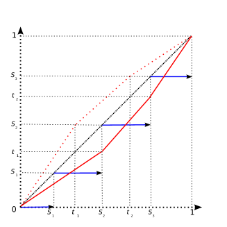
Figure 5: Lemma 6.31. Comparing the blue graph of the function $\kappa$ to the red graph of the function $\lambda^{-1}$.

Example 6.32.

Let $x_{n}(t)=1_{\{t\in[t_{0},t_{0}+2^{-n})\}}$. Since $d(x_{n},x_{n+1})=2^{-n}-2^{-n-1}=2^{-n-1}$, the sequence $(x_{n})$ is fundamental. However, it is not $d$-convergent. Indeed, $x_{n}(t)\to 0$ for all $t\neq t_{0}$ and Skorokhod convergence $x_{n}\to x$ in ${\boldsymbol{D}}$ by Lemma 6.27, should imply $x(t)=0$ for all points of continuity of $x$. Since $x\in{\boldsymbol{D}}$ has at most countably many points of discontinuities, by right continuity we conclude that $x\equiv 0$. Moreover, since the limit $x\equiv 0$ is continuous, we must have $\|x_{n}-x\|\to 0$. But $\|x_{n}\|\equiv 1$.

Theorem 6.33.

The space $\boldsymbol{D}$ is separable under $d$ and $d^{\circ}$, and is complete under $d^{\circ}$.

Proof. $Separability$ for $d$. Put $s_{j}=j/k$, $j=1,\ldots,k$. Let $B_{k}$ be the set of functions having a constant, rational value over each $[s_{j-1},s_{j})$ and a rational value at $t=1$. Then $B=\cup B_{k}$ is countable. Now it is enough to prove that given $x\in{\boldsymbol{D}}$ and $\epsilon>0$ we can find some $y\in B$ such that $d(x,y)<2\epsilon$. Choosing $k$ such that $k^{-1}<\epsilon$ and $w^{\prime}_{x}(k^{-1})<\epsilon$ we can find $y\in B_{k}$ satisfying $d(x\kappa,y)<\epsilon$, for $\kappa$ defined as in Lemma 6.31. It remains to see that $d(x\kappa,x)<\epsilon$ according to Lemma 6.31.

$Completeness$. We show that any $d^{\circ}$-fundamental sequence $x_{n}\in\boldsymbol{D}$ contains a subsequence $y_{k}=x_{n_{k}}$ that is $d^{\circ}$-convergent. Choose $n_{k}$ in such a way that $d^{\circ}(y_{k},y_{k+1})<2^{-k}$. Then $\Lambda$ contains $\mu_{k}$ such that $\|\mu_{k}\|^{\circ}<2^{-k}$ and $\|y_{k}\mu_{k}-y_{k+1}\|<2^{-k}$.

We suggest a choice of $\lambda_{k}\in\Lambda$ such that $\|\lambda_{k}\|^{\circ}\to 0$ and $\|y_{k}\lambda_{k}-y\|\to 0$ for some $y\in\boldsymbol{D}$. To this end put $\mu_{k,m}=\mu_{k}\mu_{k+1}\ldots\mu_{k+m}$. From

$$\|\mu_{k,m+1}-\mu_{k,m}\| \leq\|\mu_{k+m+1}-1\|\cdot e^{\|\mu_{k}\mu_{k+1}\ldots\mu_{k+m}\|^{\circ}}$$

$$\leq(e^{\|\mu_{k+m+1}\|^{\circ}}-1)\cdot e^{\|\mu_{k}\|^{\circ}+\ldots+\|\mu_{k+m}\|^{\circ}}$$

$$\leq 2^{-k-m}\cdot e^{2^{-k}+\ldots+2^{-k-m}}<2^{-k-m+2}$$

we conclude that for a fixed $k$ the sequence of functions $\mu_{k,m}$ is uniformly fundamental. Thus there exists a $\lambda_{k}$ such that $\|\mu_{k,m}-\lambda_{k}\|\to 0$ as $m\to\infty$. To prove that $\lambda_{k}\in\Lambda$ we use

$$\log\Big{|}{\mu_{k,m}t-\mu_{k,m}s\over t-s}\Big{|}\leq\|\mu_{k}\mu_{k+1}\ldots\mu_{k+m}\|^{\circ}<2^{-k+1}.$$

Letting here $m\to\infty$ we get $\|\lambda_{k}\|^{\circ}\leq 2^{-k+1}$. Since $\|\lambda_{k}\|^{\circ}$ is finite we conclude that $\lambda_{k}$ is strictly increasing and therefore $\lambda_{k}\in\Lambda$.

Finally, observe that

$$\|y_{k}\lambda_{k}-y_{k+1}\lambda_{k+1}\|=\|y_{k}\mu_{k}\lambda_{k+1}-y_{k+1}\lambda_{k+1}\|=\|y_{k}\mu_{k}-y_{k+1}\|<2^{-k}.$$

It follows, that the sequence $y_{k}\lambda_{k}\in\boldsymbol{D}$ is uniformly fundamental and hence $\|y_{k}\lambda_{k}-y\|\to 0$ for some $y$. Observe that $y$ must lie in $\boldsymbol{D}$. Since $\|\lambda_{k}\|^{\circ}\to 0$, we obtain $d^{\circ}(y_{k},y)\to 0$.

6.4 Relative compactness in the Skorokhod topology

First comes an analogue of the Arzela-Ascoli theorem in terms of $w^{\prime}_{x}(\delta)$, and then a convenient alternative in terms of $w^{\prime\prime}_{x}(\delta)$.

Theorem 6.34.

A set $A\subset\boldsymbol{D}$ is relatively compact in the Skorokhod topology iff

$$(i) \quad\sup_{x\in A}\|x\|<\infty,$$

$$(ii) \quad\operatorname*{\vphantom{p}lim}_{\delta\to 0}\sup_{x\in A}w^{\prime}_{x}(\delta)=0.$$

Proof of sufficiency only. Put $\alpha=\sup_{x\in A}\|x\|$. For a given $\epsilon>0$,

put $H_{\epsilon}=\{\alpha_{i}\}$, where $-\alpha=\alpha_{0}<\alpha_{1}<\ldots<\alpha_{k}=\alpha$ and $\alpha_{j}-\alpha_{j-1}\leq\epsilon$,

and choose $\delta<\epsilon$ so that $w^{\prime}_{x}(\delta)<\epsilon$ for all $x\in A$.

According to Lemma 6.31 for any $\kappa=\kappa_{\{s_{j}\}}$ satisfying $\operatorname*{\vphantom{p}max}_{j}(s_{j-1}-s_{j})\leq\delta$, we have $d(x\kappa,x)\leq\epsilon$ for all $x\in A$. Take $B_{\epsilon}$ be the set of $y\in\boldsymbol{D}$ that assume on each $[s_{j-1},s_{j})$ a constant value from $H_{\epsilon}$ and $y(1)\in H_{\epsilon}$. For any $x\in A$ there is a $y\in B_{\epsilon}$ such that $d(x\kappa,y)\leq\epsilon$. Thus $B_{\epsilon}$ forms a $2\epsilon$-net for $A$ in the sense of $d$ and $A$ is totally bounded in the sense of $d$.

But we must show that $A$ is totally bounded in the sense of $d^{\circ}$, since this is the metric under which $\boldsymbol{D}$ is complete. This is true as according Lemma 6.33, the set $B_{\delta^{2}}$ is an $\epsilon^{\prime}$-net for $A$, where $\epsilon^{\prime}=4\delta+\sup_{x\in A}w^{\prime}_{x}(\delta)$ can be chosen arbitrary small.

Theorem 6.35.

A set $A\subset\boldsymbol{D}$ is relatively compact in the Skorokhod topology iff

$$(i) \quad\sup_{x\in A}\|x\|<\infty,$$

$$(ii) \quad\left\{\begin{array}[]{l}\operatorname*{\vphantom{p}lim}_{\delta\to 0}\sup_{x\in A}w^{\prime\prime}_{x}(\delta)=0,\\ \operatorname*{\vphantom{p}lim}_{\delta\to 0}\sup_{x\in A}|x(\delta)-x(0)|=0,\\ \operatorname*{\vphantom{p}lim}_{\delta\to 0}\sup_{x\in A}|x(1-)-x(1-\delta)|=0.\end{array}\right.$$

Proof. It is enough to show that (ii) of Theorem 6.35 is equivalent to (ii) of Theorem 6.34. This follows from Lemma 6.14.

7 Probability measures on $\boldsymbol{D}$ and random elements

7.1 Finite-dimensional distributions on $\boldsymbol{D}$

Finite-dimensional sets play in $\boldsymbol{D}$ the same role as they do in $\boldsymbol{C}$.

Definition 7.1.

Consider projection mappings $\pi_{t_{1},\ldots,t_{k}}:\boldsymbol{D}\to\boldsymbol{R}^{k}$. For $T\subset[0,1]$, define in $\mathcal{D}$ the subclass $\mathcal{D}_{f}(T)$ of finite-dimensional sets $\pi_{t_{1},\ldots,t_{k}}^{-1}(H)$, where $k$ is arbitrary, $t_{i}$ belong to $T$, and $H\in\mathcal{R}^{k}$.

Theorem 7.2.

Consider projection mappings $\pi_{t_{1},\ldots,t_{k}}:\boldsymbol{D}\to\boldsymbol{R}^{k}$. The following three statements hold.

(a) The projections $\pi_{0}$ and $\pi_{1}$ are continuous, and for $t\in(0,1)$, $\pi_{t}$ is continuous at $x$ if and only if $x$ is continuous at $t$.

(b) Each $\pi_{t_{1},\ldots,t_{k}}$ is a measurable map.

(c) If $T$ contains 1 and is dense in $[0,1]$, then $\sigma\{\pi_{t}:t\in T\}=\sigma\{\mathcal{D}_{f}(T)\}=\mathcal{D}$ and $\mathcal{D}_{f}(T)$ is a separating class.

Proof. (a) Since each $\lambda\in\Lambda$ fixes 0 and 1, $\pi_{0}$ and $\pi_{1}$ are continuous: for $i=0,1$,

$$d(x,y)\geq\operatorname*{\vphantom{p}inf}_{\lambda\in\Lambda}\|x-y\lambda\|\geq|x(i)-y(i)|=|\pi_{i}(x)-\pi_{i}(y)|.$$

Suppose that $0<t<1$. If $x$ is continuous at $t$, then by Lemma 6.27, $\pi_{t}$ is continuous at $x$. Suppose, on the other hand, that $x$ is discontinuous at $t$. If $\lambda_{n}\in\Lambda$ carries $t$ to $t-1/n$ and is linear on $[0,t]$ and $[t,1]$, and if $x_{n}(s)=x(\lambda_{n}s)$, then $d(x_{n},x)\to 0$ but $x_{n}(t)\nrightarrow x(t)$.

(b) A mapping into $\boldsymbol{R}^{k}$ is measurable if each component mapping is. Therefore it suffices to show that $\pi_{t}$ is measurable. Since $\pi_{1}$ is continuous, we may assume $t<1$. We use the pointwise convergence

$$h_{\epsilon}(x):=\epsilon^{-1}\int_{t}^{t+\epsilon}x_{s}ds\to\pi_{t}(x),\quad\epsilon\to 0,\quad x\in\boldsymbol{D}.$$

If $x^{n}\to x$ in the Skorokhod topology, then $x^{n}_{t}\to x_{t}$ for continuity points $t$ of $x$, and we conclude that $x^{n}\to x$ almost surely. By the Bounded Convergence Theorem, the almost sure convergence $x^{n}\to x$ and the uniform boundedness of $(x^{n})$ imply $h_{\epsilon}(x^{n})\to h_{\epsilon}(x)$. Thus for each $\epsilon$, $h_{\epsilon}$ is continuous and therefore measurable, implying that its limit $\pi_{t}$ is also measurable.

(c) By right-continuity and the assumption that $T$ is dense, it follows that $\pi_{0}$ is measurable with respect to $\sigma\{\mathcal{D}_{f}(T)\}$. So we may as well assume that $0\in T$.

Suppose $s_{0},\ldots,s_{k}$ are points in $T$ satisfying $0=s_{0}<\ldots<s_{k}=1$. For $\alpha=(\alpha_{0},\ldots,\alpha_{k})\in\boldsymbol{R}^{k+1}$ define $V\alpha\in\boldsymbol{D}$ by

$$(V\alpha)(t)=\left\{\begin{array}[]{ll}\alpha_{j-1}&\mbox{for }t\in[s_{j-1},s_{j}),\ j=1,\ldots,k,\\ \alpha_{k}&\mbox{for }t=1.\end{array}\right.$$

Clearly, $V:\boldsymbol{R}^{k+1}\to\boldsymbol{D}$ is continuous implying that $\kappa=V\pi_{s_{0},\ldots,s_{k}}$ is measurable $\sigma\{\mathcal{D}_{f}(T)\}/\mathcal{D}$.

Since $T$ is dense, for any $n$ we can choose $s_{0}^{n},\ldots,s_{k}^{n}$ so that $\operatorname*{\vphantom{p}max}_{i}(s_{i}^{n}-s_{i-1}^{n})<n^{-1}$. Put $\kappa^{n}=V\pi_{s_{0}^{n},\ldots,s_{k}^{n}}$. With this choice define a map $A_{n}:\boldsymbol{D}\to\boldsymbol{D}$ by $A_{n}x=x\kappa^{n}$. By Lemma 6.31, $A_{n}x\to x$ for each $x$. We conclude that the identity map is measurable $\sigma\{\mathcal{D}_{f}(T)\}/\mathcal{D}$ and therefore $\mathcal{D}\subset\sigma\{\mathcal{D}_{f}(T)\}$. Finally, since $\mathcal{D}_{f}(T)$ is a $\pi$-system, it is a separating class.

Definition 7.3.

Let $D_{c}$ be the set of count paths: nondecreasing functions $x\in\boldsymbol{D}$ with $x(t)\in\mathbb{Z}$ for each $t$, and $x(t)-x(t-)=1$ at points of discontinuity.

Exercise 7.4.

Find $d(x,y)$ for $x,y\in D_{c}$ in terms of the jump points of these two count paths. How does a fundamental sequence $(x_{n})$ in $D_{c}$ look for large $n$? Show that $D_{c}$ is closed in the Skorokhod topology.

Lemma 7.5.

Let $T_{0}=\{t_{1},t_{2},\ldots\}$ be a countable, dense set in $[0,1]$, and put $\pi(x)=(x(t_{1}),x(t_{2}),\ldots).$

(a) The mapping $\pi:\boldsymbol{D}\to\boldsymbol{R}^{\infty}$ is $\mathcal{D}/\mathcal{R}^{\infty}$-measurable.

(b) If $x,x_{n}\in D_{c}$ are such that $\pi(x_{n})\to\pi(x)$, then $x_{n}\to x$ in the Skorokhod topology.

Proof. (a) In terms of notation of Section 2.3,

$$\pi^{-1}(\pi^{-1}_{k}H)=\pi^{-1}_{t_{1},\ldots,t_{k}}H\in\mathcal{D}\qquad\mbox{ for }H\in\mathcal{R}^{k},$$

and the finite-dimensional sets $\pi^{-1}_{k}H$ generate $\mathcal{R}^{\infty}$.

(b) Convergence $\pi(x_{n})\to\pi(x)$ implies $x_{n}(t_{i})\to x(t_{i})$, which in turn means that $x_{n}(t_{i})=x(t_{i})$ for $n>n_{i}$, for all $i=1,2,\ldots$. A function in $x\in D_{c}$ has only finitely many discontinuities, say $0<s_{1}<\ldots<s_{k}\leq 1$. For a given $\epsilon$ choose points $u_{i}$ and $v_{i}$ in $T_{0}$ in such a way that $u_{i}<s_{i}\leq v_{i}<u_{i}+\epsilon$ and the intervals $[v_{i-1},u_{i}],i=1,\ldots,k$ are disjoint, with $v_{0}=0$. Then for $n$ exceeding some $n_{0}$, $x_{n}$ agrees with $x$ over each $[v_{i-1},u_{i}]$ and has a single jump in each $[u_{i},v_{i}]$. If $\lambda_{n}\in\Lambda$ carries $s_{i}$ to the point in $[u_{i},v_{i}]$ where $x_{n}$ has a jump and is defined elsewhere by linearity, then $\|\lambda_{n}-1\|\leq\epsilon$ and $x_{n}(\lambda_{n}t)\equiv x(t)$ implying $d(x_{n},x)\leq\epsilon$ for $n>n_{0}$.

Theorem 7.6.

Let $T_{0}$ be a countable, dense set in $[0,1]$. If $P_{n}(D_{c})=P(D_{c})=1$ and $P_{n}\pi^{-1}_{t_{1},\ldots,t_{k}}\Rightarrow P\pi^{-1}_{t_{1},\ldots,t_{k}}$ for all $k$-tuples in $T_{0}$, then $P_{n}\Rightarrow P$.

Proof. The idea is, in effect, to embed $D_{c}$ in $\boldsymbol{R}^{\infty}$ and apply Theorem 2.14. By hypothesis, $P_{n}\pi^{-1}\pi^{-1}_{k}\Rightarrow P\pi^{-1}\pi^{-1}_{k}$, but since in $\boldsymbol{R}^{\infty}$ weak convergence is the same thing as weak convergence of finite-dimensional distributions, it follows that $P_{n}\pi^{-1}\Rightarrow P\pi^{-1}$ in $\boldsymbol{R}^{\infty}$. For $A\subset\boldsymbol{D}$, define $A^{*}=\pi^{-1}(\pi A)^{-}$. If $A\in\mathcal{D}$, then

$$\limsup_{n}P_{n}(A)\leq\limsup_{n}P_{n}(A^{*})=\limsup_{n}P_{n}(\pi^{-1}(\pi A)^{-})\leq P(\pi^{-1}(\pi A)^{-})=P(A^{*}).$$

Therefore, if $F\in\mathcal{D}$ is closed, then

$$\limsup_{n}P_{n}(F)=\limsup_{n}P_{n}(F\cap D_{c})\leq P((F\cap D_{c})^{*})=P((F\cap D_{c})^{*}\cap D_{c}).$$

It remains to show that if $F\in\mathcal{D}$ is closed, then $(F\cap D_{c})^{*}\cap D_{c}\subset F$. Take an $x\in(F\cap D_{c})^{*}\cap D_{c}$. Since $x\in(F\cap D_{c})^{*}$, we have $\pi(x)\in(\pi(F\cap D_{c}))^{-}$ and there is a sequence $x_{n}\in F\cap D_{c}$ such that $\pi(x_{n})\to\pi(x)$. Because $x\in D_{c}$, the previous lemma gives $x_{n}\to x$ in the Skorokhod topology. Since $x_{n}\in F$ and $F\in\mathcal{D}$ is closed, we conclude that $x\in F$.

Corollary 7.7.

Suppose for each $n$, $\xi_{n1},\ldots,\xi_{nn}$ are iid indicator r.v. with $\mathbb{P}(\xi_{ni}=1)=\alpha/n$. If $X^{n}_{t}=\sum_{i\leq nt}\xi_{ni}$, then $X^{n}\Rightarrow X$ in $\boldsymbol{D}$, where $X$ is the Poisson process with parameter $\alpha$.

Proof. The random process $X^{n}_{t}=\sum_{i\leq nt}\xi_{ni}$ has independent increments. Its finite-dimensional distributions weakly converge to that of the Poisson process $X$ with

$$\mathbb{P}(X_{t}-X_{s}=k)={\alpha^{k}(t-s)^{k}\over k!}e^{-\alpha(t-s)}\qquad\mbox{ for }0\leq s<t\leq 1.$$

Exercise 7.8.

Suppose that $\xi$ is uniformly distributed over $[{1\over 3},{2\over 3}]$, and consider the random functions

$$X_{t}=2\cdot 1_{\{t\in[\xi,1]\}},\quad X_{t}^{n}=1_{\{t\in[\xi-n^{-1},1]\}}+1_{\{t\in[\xi+n^{-1},1]\}}.$$

Show that $X^{n}\nRightarrow X$, even though $(X^{n}_{t_{1}},\ldots,X^{n}_{t_{k}})\Rightarrow(X_{t_{1}},\ldots,X_{t_{k}})$ for all $(t_{1},\ldots,t_{k})$. Why does Theorem 7.6 not apply?

Lemma 7.9.

Let $P$ be a probability measure on $(\boldsymbol{D},\mathcal{D})$. Define $T_{P}\subset[0,1]$ as the collection of $t$ such that the projection $\pi_{t}$ is $P$-almost surely continuous. The set $T_{P}$ contains 0 and 1, and its complement in $[0,1]$ is at most countable. For $t\in(0,1)$, $t\in T_{P}$ is equivalent to $P\{x:x(t)\neq x(t-)\}=0$.

Proof. Recall Theorem 7.2 (a) and put $J_{t}=\{x:x(t)\neq x(t-)\}$ for a $t\in(0,1)$. We have to show that $P(J_{t})>0$ is possible for at most countably many $t$. Let $J_{t}(\epsilon)=\{x:|x(t)-x(t-)|>\epsilon\}$. For fixed, positive $\epsilon$ and $\delta$, there can be at most finitely many $t$ for which $P(J_{t}(\epsilon))\geq\delta$. Indeed, if $P(J_{t_{n}}(\epsilon))\geq\delta$ for infinitely many distinct $t_{n}$, then

$$P(J_{t_{n}}(\epsilon)\mbox{ i.o.})=P(\limsup_{n}J_{t_{n}}(\epsilon))\geq\limsup_{n\to\infty}P(J_{t_{n}}(\epsilon))\geq\delta,$$

contradicting the fact that for a single $x\in\boldsymbol{D}$ the jumps can exceed $\epsilon$ at only finitely many points, see Lemma 6.4. Thus $P(J_{t}(\epsilon))>0$ is possible for at most countably many $t$. The desired result follows from

$$\{t:P(J_{t})>0\}=\bigcup_{n}\{t:P(J_{t}(n^{-1}))>0\},$$

which in turn is a consequence of $P(J_{t}(\epsilon))\uparrow P(J_{t})$ as $\epsilon\downarrow 0$.

Theorem 7.10.

Let $P_{n},P$ be probability measures on $(\boldsymbol{D},\mathcal{D})$. If the sequence $(P_{n})$ is tight and $P_{n}\pi^{-1}_{t_{1},\ldots,t_{k}}\Rightarrow P\pi^{-1}_{t_{1},\ldots,t_{k}}$ holds whenever $t_{1},\ldots,t_{k}$ lie in $T_{P}$, then $P_{n}\Rightarrow P$.

Proof. We will show that if a subsequence $(P_{n^{\prime}})\subset(P_{n})$ converges weakly to some $Q$, then $Q=P$. Indeed, if $t_{1},\ldots,t_{k}$ lie in $T_{Q}$, then $\pi_{t_{1},\ldots,t_{k}}$ is continuous on a set of $Q$-measure 1, and therefore, $P_{n^{\prime}}\Rightarrow Q$ implies by the mapping theorem that $P_{n^{\prime}}\pi^{-1}_{t_{1},\ldots,t_{k}}\Rightarrow Q\pi^{-1}_{t_{1},\ldots,t_{k}}$. On the other hand, if $t_{1},\ldots,t_{k}$ lie in $T_{P}$, then $P_{n^{\prime}}\pi^{-1}_{t_{1},\ldots,t_{k}}\Rightarrow P\pi^{-1}_{t_{1},\ldots,t_{k}}$ by the assumption. Therefore, if $t_{1},\ldots,t_{k}$ lie in $T_{Q}\cap T_{P}$, then $Q\pi^{-1}_{t_{1},\ldots,t_{k}}=P\pi^{-1}_{t_{1},\ldots,t_{k}}$. It remains to see that $\mathcal{D}_{f}(T_{Q}\cap T_{P})$ is a separating class by applying Lemma 7.9 and Theorem 7.2.

7.2 Tightness criteria in $\boldsymbol{D}$

Theorem 7.11.

Let $P_{n}$ be probability measures on $(\boldsymbol{D},\mathcal{D})$. The sequence $(P_{n})$ is tight if and only if the following two conditions hold:

$$(i) \quad\operatorname*{\vphantom{p}lim}_{a\to\infty}\limsup_{n\to\infty}P_{n}(x:\|x\|\geq a)=0,$$

$$(ii) \quad\operatorname*{\vphantom{p}lim}_{\delta\to 0}\limsup_{n\to\infty}P_{n}(x:w^{\prime}_{x}(\delta)\geq\epsilon)=0,\mbox{ for each positive }\epsilon.$$

Condition (ii) is equivalent to

$$(ii^{\prime}) \quad\forall\epsilon,\eta>0;\exists\delta,n_{0}>0:\quad P_{n}(x:w^{\prime}_{x}(\delta)\geq\epsilon)\leq\eta,\mbox{ for }n>n_{0}.$$

Proof. This theorem is proven similarly to Theorem 4.25 using Theorem 6.34. Equivalence of (ii) and (ii^′) is due to monotonicity of $w^{\prime}_{x}(\delta)$.

Theorem 7.12.

Let $P_{n}$ be probability measures on $(\boldsymbol{D},\mathcal{D})$. The sequence $(P_{n})$ is tight if and only if the following two conditions hold:

$$(i) \quad\operatorname*{\vphantom{p}lim}_{a\to\infty}\limsup_{n\to\infty}P_{n}(x:\|x\|\geq a)=0,$$

$$(ii) \quad\forall\epsilon,\eta>0;\exists\delta,n_{0}>0:\quad\left\{\begin{array}[]{l}P_{n}(x:w^{\prime\prime}_{x}(\delta)\geq\epsilon)\leq\eta,\\ P_{n}(x:|x(\delta)-x(0)|\geq\epsilon)\leq\eta,\\ P_{n}(x:|x(1-)-x(1-\delta)|\geq\epsilon)\leq\eta,\end{array}\right.\quad\mbox{ for }n>n_{0}.$$

Proof. This theorem follows from Theorem 7.11 with $(i)$ and $(ii^{\prime})$ using Lemma 6.14. (Recall how Theorem 6.35 was obtained from Theorem 6.34 using Lemma 6.14.)

Lemma 7.13.

Turn to Theorems 7.11 and 7.12. Under (ii) condition (i) is equivalent to the following weaker version:

(i$\,{}^{\prime}$) for each $t$ in a set $T$ that is dense in $[0,1]$ and contains 1,

$$\operatorname*{\vphantom{p}lim}_{a\to\infty}\limsup_{n\to\infty}P_{n}(x:|x(t)|\geq a)=0,$$

Proof. The implication (i) $\Rightarrow$ (i^′) is trivial. Assume (ii) of Theorem 7.11 and (i^′). For a given $\delta\in(0,1)$ choose from $T$ points $0<s_{1}<\ldots<s_{k}=1$ such that $\operatorname*{\vphantom{p}max}\{s_{1},s_{2}-s_{1},\ldots,s_{k}-s_{k-1}\}<\delta$. By hypothesis (i^′), there exists an $a$ such that

$$\qquad\qquad\qquad\qquad P_{n}(x:\operatorname*{\vphantom{p}max}_{j}|x(s_{j})|\geq a)<\eta,\quad n>n_{0}\qquad\qquad\qquad\qquad(*)$$

For a given $x$, take a $\delta$-sparse set $(t_{0},\ldots,t_{v})$ such that all $w_{x}[t_{i-1},t_{i})<w^{\prime}_{x}(\delta)+1$. Since each $[t_{i-1},t_{i})$ contains an $s_{j}$, we have

$$\|x\|\leq\operatorname*{\vphantom{p}max}_{j}|x(s_{j})|+w^{\prime}_{x}(\delta)+1.$$

Using (ii^′) of Theorem 7.11 and $(*)$, we get $P_{n}(x:\|x\|\geq a+2)<2\eta$ implying (i).

7.3 A key condition on 3-dimensional distributions

The following condition plays an important role.

Definition 7.14.

For a probability measure $P$ on $\boldsymbol{D}$, we will write $P\in H_{\alpha,\beta}$, if there exist $\alpha>1$, $\beta\geq 0$, and a nondecreasing continuous $H:[0,1]\to\boldsymbol{R}$ such that for all $\epsilon>0$ and all $0\leq t_{1}\leq t_{2}\leq t_{3}\leq 1$,

$$P\pi^{-1}_{t_{1},t_{2},t_{3}}\{(z_{1},z_{2},z_{3}):|z_{2}-z_{1}|\geq\epsilon,|z_{3}-z_{2}|\geq\epsilon\}\leq\epsilon^{-2\beta}(H(t_{3})-H(t_{1}))^{\alpha}.$$

For a random element $X$ on $\boldsymbol{D}$ with probability distribution $P$, this condition $P\in H_{\alpha,\beta}$ means that for all $\epsilon>0$ and all $0\leq r\leq s\leq t\leq 1$

$$\mathbb{P}\Big{(}|X_{s}-X_{r}|\geq\epsilon,|X_{t}-X_{s}|\geq\epsilon\Big{)}\leq\epsilon^{-2\beta}(H(t)-H(r))^{\alpha}.$$

Lemma 7.15.

Let a random element $X$ on $\boldsymbol{D}$ have a probability distribution $P\in H_{\alpha,\beta}$. Then there is a constant $K_{\alpha,\beta}$ depending only on $\alpha$ and $\beta$ such that

$$\mathbb{P}\Big{(}\sup_{r\leq s\leq t}\big{(}|X_{s}-X_{r}|\wedge|X_{t}-X_{s}|\big{)}\geq\epsilon\Big{)}\leq{K_{\alpha,\beta}\over\epsilon^{2\beta}}(H(1)-H(0))^{\alpha}.$$

Proof. The stated estimate is obtained in four consecutive steps.

Step 1. Let $T_{k}=\{i/2^{k},0\leq i\leq 2^{k}\}$ and

$$A_{k} =\operatorname*{\vphantom{p}max}\big{(}|X_{s}-X_{r}|\wedge|X_{t}-X_{s}|\mbox{ over the adjacent triplets }r\leq s\leq t\mbox{ in }T_{k}\big{)},$$

$$B_{k} =\operatorname*{\vphantom{p}max}\big{(}|X_{s}-X_{r}|\wedge|X_{t}-X_{s}|\mbox{ over }r\leq s\leq t\mbox{ from }T_{k}\big{)}.$$

We will show that $B_{k}\leq 2(A_{1}+\ldots+A_{k})$. To this end, for each $t\in T_{k}$ define a $t_{n}\in T_{k-1}$ by

$$t_{n}=\left\{\begin{array}[]{ll}t&\mbox{if }t\in T_{k-1},\\ t-2^{-k}&\mbox{if }t\notin T_{k-1}\mbox{ and }|X_{t}-X_{t-2^{-k}}|\leq|X_{t}-X_{t+2^{-k}}|,\\ t+2^{-k}&\mbox{if }t\notin T_{k-1}\mbox{ and }|X_{t}-X_{t-2^{-k}}|>|X_{t}-X_{t+2^{-k}}|,\end{array}\right.$$

so that $|X_{t}-X_{t_{n}}|\leq A_{k}$. Then for any triplet $r\leq s\leq t$ from $T_{k}$,

$$|X_{s}-X_{r}| \leq|X_{s}-X_{s_{n}}|+|X_{s_{n}}-X_{r_{n}}|+|X_{r}-X_{r_{n}}|\leq|X_{s_{n}}-X_{r_{n}}|+2A_{k},$$

$$|X_{t}-X_{s}| \leq|X_{t_{n}}-X_{s_{n}}|+2A_{k}.$$

Since here $r_{n}\leq s_{n}\leq t_{n}$ lie in $T_{k-1}$, it follows that $|X_{s}-X_{r}|\wedge|X_{t}-X_{s}|\leq B_{k-1}+2A_{k}$, and therefore,

$$B_{k}\leq B_{k-1}+2A_{k}\leq 2(A_{1}+\ldots+A_{k}),\quad k\geq 1.$$

Step 2. Consider a special case when $H(t)\equiv t$. Using the right continuity of the paths we get from step 1 that

$$\sup_{r\leq s\leq t}\big{(}|X_{s}-X_{r}|\wedge|X_{t}-X_{s}|\big{)}\leq 2\sum_{k=1}^{\infty}A_{k}.$$

This implies that for any $\theta\in(0,1)$,

$$\mathbb{P}\Big{(}\sup_{r\leq s\leq t}\big{(}|X_{s}-X_{r}| \wedge|X_{t}-X_{s}|\big{)}\geq 2\epsilon\Big{)}\leq\mathbb{P}\Big{(}\sum_{k=1}^{\infty}A_{k}\geq\epsilon\Big{)}$$

$$\leq\mathbb{P}\Big{(}\sum_{k=1}^{\infty}A_{k}\geq\epsilon(1-\theta)\sum_{k=1}^{\infty}\theta^{k}\Big{)}\leq\sum_{k=1}^{\infty}\mathbb{P}\Big{(}A_{k}\geq\epsilon(1-\theta)\theta^{k}\Big{)}$$

$$\leq\sum_{k=1}^{\infty}\sum_{i=1}^{2^{k}-1}\mathbb{P}\Big{(}|X_{i/2^{k}}-X_{(i-1)/2^{k}}|\wedge|X_{(i+1)/2^{k}}-X_{i/2^{k}}|\geq\epsilon(1-\theta)\theta^{k}\Big{)}.$$

Applying the key condition with $H(t)\equiv t$ we derive from the previous relation choosing a $\theta\in(0,1)$ satisfying $\theta^{2\beta}>2^{1-\alpha}$, that the stated estimate holds in the special case

$$\mathbb{P}\Big{(}\sup_{r\leq s\leq t}\big{(}|X_{s}-X_{r}|\wedge|X_{t}-X_{s}|\big{)}\geq 2\epsilon\Big{)} \leq\sum_{k=1}^{\infty}2^{k}{2^{(1-k)\alpha}\over(\epsilon(1-\theta)\theta^{k})^{2\beta}}$$

$$={2^{\alpha}\over\epsilon^{2\beta}(1-\theta)^{2\beta}}\sum_{k=1}^{\infty}(\theta^{-2\beta}2^{1-\alpha})^{k}.$$

Step 3. For a strictly increasing $H(t)$ take $a$ so that $a^{2\beta}H(1)^{\alpha}=1$, and define a new process $Y_{t}$ by $Y_{t}=aX_{b(t)}$, where the time change $b(t)$ is such that $H(b(t))=tH(1)$. Since

$$\mathbb{P}\Big{(}|Y_{s}-Y_{r}|\geq\epsilon;|Y_{t}-Y_{s}|\geq\epsilon\Big{)} =\mathbb{P}\Big{(}|X_{b(s)}-X_{b(r)}|\geq a^{-1}\epsilon;|X_{b(t)}-X_{b(s)}|\geq a^{-1}\epsilon\Big{)}$$

$$\leq\epsilon^{-2\beta}(t-r)^{\alpha},$$

we can apply the result of the step 2 to the new process and prove the statement of the lemma under the assumption of step 3.

Step 4. If $H(t)$ is not strictly increasing, put $H_{v}(t)=H(t)+vt$ for an arbitrary small positive $v$. We have

$$\mathbb{P}\Big{(}|X_{s}-X_{r}|\geq\epsilon;|X_{t}-X_{s}|\geq\epsilon\Big{)}\leq\epsilon^{-2\beta}(H_{v}(t)-H_{v}(r))^{\alpha},$$

and according to step 3

$$\mathbb{P}\Big{(}\sup_{r\leq s\leq t}\big{(}|X_{s}-X_{r}|\wedge|X_{t}-X_{s}|\big{)}\geq\epsilon\Big{)}\leq{K_{\alpha,\beta}\over\epsilon^{2\beta}}(H(1)+v-H(0))^{\alpha}.$$

It remains to let $v$ go to 0. Lemma 7.15 is proven.

Lemma 7.16.

If $P\in H_{\alpha,\beta}$, then given a positive $\epsilon$,

$$P(x:w^{\prime\prime}_{x}(\delta)\geq\epsilon)\leq{2K_{\alpha,\beta}\over\epsilon^{2\beta}}(H(1)-H(0))(w_{H}(2\delta))^{\alpha-1},$$

so that $P(x:w^{\prime\prime}_{x}(\delta)\geq\epsilon)\to 0$ as $\delta\to 0$.

Proof. Take $t_{i}=i\delta$ for $0\leq i\leq\lfloor 1/\delta\rfloor$ and $t_{\lceil 1/\delta\rceil}=1$. If $|t-r|\leq\delta$, then $r$ and $t$ lie in the same $[t_{i-1},t_{i+1}]$ for some $1\leq i\leq\lceil 1/\delta\rceil-1$. According to Lemma 7.15, for $X$ with distribution $P$,

$$\mathbb{P}\Big{(}\sup_{t_{i-1}\leq r\leq s\leq t\leq t_{i+1}}\big{(}|X_{s}-X_{r}|\wedge|X_{t}-X_{s}|\big{)}\geq\epsilon\Big{)}\leq{K_{\alpha,\beta}\over\epsilon^{2\beta}}(H(t_{i+1})-H(t_{i-1}))^{\alpha},$$

and due to monotonicity of $H$,

$$\mathbb{P}\Big{(}w^{\prime\prime}(X,\delta)\geq\epsilon\Big{)} \leq\sum_{i=1}^{\lceil 1/\delta\rceil-1}{K_{\alpha,\beta}\over\epsilon^{2\beta}}(H(t_{i+1})-H(t_{i-1}))^{\alpha}$$

$$\leq{K_{\alpha,\beta}\over\epsilon^{2\beta}}\Big{(}\sup_{0\leq t\leq 1-2\delta}(H(t+2\delta)-H(t))^{\alpha-1}\Big{)}2(H(1)-H(0))$$

$$={2K_{\alpha,\beta}\over\epsilon^{2\beta}}(H(1)-H(0))(w_{H}(2\delta))^{\alpha-1}.$$

It remains to recall that the modulus of continuity $w_{H}(2\delta)$ of the uniformly continuous function $H$ converges to 0 as $\delta\to 0$.

7.4 A criterion for existence

Theorem 7.17.

There exists in $\boldsymbol{D}$ a random element with finite dimensional distributions $\mu_{t_{1},\ldots,t_{k}}$ provided the following three conditions:

(i) the finite dimensional distributions $\mu_{t_{1},\ldots,t_{k}}$ are consistent, see Definition 2.15,

(ii) there exist $\alpha>1$, $\beta\geq 0$, and a nondecreasing continuous $H:[0,1]\to\boldsymbol{R}$ such that for all $\epsilon>0$ and all $0\leq t_{1}\leq t_{2}\leq t_{3}\leq 1$,

$$\mu_{t_{1},t_{2},t_{3}}\{(z_{1},z_{2},z_{3}):|z_{2}-z_{1}|\geq\epsilon,|z_{3}-z_{2}|\geq\epsilon\}\leq\epsilon^{-2\beta}(H(t_{3})-H(t_{1}))^{\alpha},$$

(iii) $\mu_{t,t+\delta}\{(z_{1},z_{2}):|z_{2}-z_{1}|\geq\epsilon\}\to 0$ as $\delta\downarrow 0$ for each $t\in[0,1)$.

Proof. The main idea, as in the proof of Theorem 4.15 (a), is to construct a sequence $(X^{n})$ of random elements in $\boldsymbol{D}$ such that the corresponding sequence of distributions $(P_{n})$ is tight and has the desired limit finite dimensional distributions $\mu_{t_{1},\ldots,t_{k}}$.

Let vector $(X_{n,0},\ldots,X_{n,2^{n}})$ have distribution $\mu_{t_{0},\ldots,t_{2^{n}}}$, where $t_{i}\equiv t^{n}_{i}=i2^{-n}$, and define

$$X^{n}_{t}=\left\{\begin{array}[]{ll}X_{n,i}&\mbox{for }t\in[i2^{-n},(i+1)2^{-n}),\quad i=0,\ldots,2^{n}-1,\\ X_{n,2^{n}}&\mbox{for }t=1.\end{array}\right.$$

The rest of the proof uses Theorem 7.12 and is divided in four steps.

Step 1. For all $\epsilon>0$ and $r,s,t\in T_{n}=\{t_{0},\ldots,t_{2^{n}}\}$ we have by (ii),

$$\mathbb{P}\Big{(}|X_{s}^{n}-X_{r}^{n}|\geq\epsilon,|X_{t}^{n}-X_{s}^{n}|\geq\epsilon\Big{)}\leq\epsilon^{-2\beta}(H(t)-H(r))^{\alpha}.$$

It follows that in general for $0\leq r\leq s\leq t\leq 1$

$$\mathbb{P}\Big{(}|X_{s}^{n}-X_{r}^{n}|\geq\epsilon,|X_{t}^{n}-X_{s}^{n}|\geq\epsilon\Big{)}\leq\epsilon^{-2\beta}(H(t)-H(r-2^{-n}))^{\alpha},$$

where $H(t)=H(0)$ for $t<0$. Slightly modifying Lemma 7.16 we obtain that given a positive $\epsilon$, there is a constant $K_{\alpha,\beta,\epsilon}$

$$P_{n}(x:w^{\prime\prime}_{x}(\delta)\geq\epsilon)\leq K_{\alpha,\beta,\epsilon}(H(1)-H(0))(w_{H}(3\delta))^{\alpha-1},\quad\mbox{for }\delta\leq 2^{-n}.$$

This gives the first part of (ii) in Theorem 7.12.

Step 2. If $2^{-k}\leq\delta$, then

$$\|X^{n}\|\leq\operatorname*{\vphantom{p}max}_{t\in T_{k}}|X^{n}_{t}|+w^{\prime\prime}(X^{n},\delta).$$

Since the distributions of the first term on the right all coincide for $n\geq k$, it follows by step 1 that condition (i) in Theorem 7.12 is satisfied.

Step 3. To take care of the second and third parts of (ii) in Theorem 7.12, we fix some $\delta_{0}\in(0,1/2)$, and temporarily assume that for $\delta\in(0,\delta_{0})$,

$$\qquad\qquad\mu_{0,\delta}\{(z_{1},z_{2}):z_{1}=z_{2}\}=1,\qquad\mu_{1-\delta,1}\{(z_{1},z_{2}):z_{1}=z_{2}\}=1.\qquad\qquad\qquad(*)$$

In this special case, the second and third parts of (ii) in Theorem 7.12 hold and we conclude that the sequence of distributions $P_{n}$ of $X_{n}$ is tight.

By Prokhorov’s theorem, $(X^{n})$ has a subsequence weakly converging in distribution to a random element $X$ of $\boldsymbol{D}$ with some distribution $P$. We want to show that $P\pi^{-1}_{t_{1},\ldots,t_{k}}=\mu_{t_{1},\ldots,t_{k}}$. Because of the consistency hypothesis, this holds for dyadic rational $t_{i}\in\cup_{n}T_{n}$. The general case is obtained using the following facts:

$$P_{n}\pi^{-1}_{t_{1},\ldots,t_{k}} \Rightarrow P\pi^{-1}_{t_{1},\ldots,t_{k}},$$

$$P_{n}\pi^{-1}_{t_{1},\ldots,t_{k}} =\mu_{t_{n1},\ldots,t_{nk}},\quad\mbox{ for some }t_{ni}\in T_{n},\mbox{ provided }k\leq 2^{n},$$

$$\mu_{t_{n1},\ldots,t_{nk}} \Rightarrow\mu_{t_{1},\ldots,t_{k}}.$$

The last fact is a consequence of (iii). Indeed, by Kolmogorov’s extension theorem, there exists a stochastic process $Z$ with vectors $(Z_{t_{1}},\ldots,Z_{t_{k}})$ having distributions $\mu_{t_{1},\ldots,t_{k}}$. Then by (iii), $Z_{t+\delta}\stackrel{{\scriptstyle\rm P}}{{\to}}Z_{t}$ as $\delta\downarrow 0$. Using Exercise 1.22 we derive $(Z_{t_{n1}},\ldots,Z_{t_{nk}})\stackrel{{\scriptstyle\rm P}}{{\to}}(Z_{t_{1}},\ldots,Z_{t_{k}})$ implying $\mu_{t_{n1},\ldots,t_{nk}}\Rightarrow\mu_{t_{1},\ldots,t_{k}}$.

Step 4. It remains to remove the restriction $(*)$. To this end take

$$\lambda t=\left\{\begin{array}[]{ll}0&\mbox{for }t\leq\delta_{0},\\ {t-\delta_{0}\over 1-2\delta_{0}}&\mbox{for }\delta_{0}<t<1-\delta_{0},\\ 1&\mbox{for }t\geq 1-\delta_{0}.\end{array}\right.$$

Define $\nu_{s_{1},\ldots,s_{k}}$ as $\mu_{t_{1},\ldots,t_{k}}$ for $s_{i}=\lambda t_{i}$. Then the $\nu_{s_{1},\ldots,s_{k}}$ satisfy the conditions of the theorem with a new $H$, as well as $(*)$, so that there is a random element $Y$ of $\boldsymbol{D}$ with these finite-dimensional distributions. Finally, setting $X_{t}=Y_{\delta_{0}+t(1-2\delta_{0})}$ we get a process $X$ with the required finite dimensional distributions $P\pi^{-1}_{t_{1},\ldots,t_{k}}=\mu_{t_{1},\ldots,t_{k}}$.

Example 7.18.

Construction of a Levy process. Let $\nu_{t}$ be a measure on the line for which $\nu_{t}(\boldsymbol{R})=H(t)$ is nondecreasing and continuous, $t\in[0,1]$. Suppose for $s\leq t$, $\nu_{s}(A)\leq\nu_{t}(A)$ for all $A\in\mathcal{R}$ so that $\nu_{t}-\nu_{s}$ is a measure with total mass $H(t)-H(s)$. Then there is an infinitely divisible distribution having mean 0, variance $H(t)-H(s)$, and characteristic function

$$\phi_{s,t}(u)=\exp\int_{-\infty}^{\infty}{e^{iuz}-1-iuz\over z^{2}}(\nu_{t}-\nu_{s})(dz).$$

We can use Theorem 7.17 to construct a random element $X$ of $\boldsymbol{D}$ with $X_{0}=0$, for which the increments are independent and

$$\mathbb{E}(e^{iu_{1}X_{t_{1}}}e^{iu_{2}(X_{t_{2}}-X_{t_{1}})}\cdots e^{iu_{k}(X_{t_{k}}-X_{t_{k-1}})})=\phi_{0,t_{1}}(u_{1})\phi_{t_{1},t_{2}}(u_{2})\cdots\phi_{t_{k-1},t_{k}}(u_{k}).$$

Indeed, since $\phi_{r,t}(u)=\phi_{r,s}(u)\phi_{s,t}(u)$ for $r\leq s\leq t$, the implied finite-dimensional distributions $\mu_{t_{1},\ldots,t_{k}}$ are consistent. Further, by Chebyshev’s inequality and independence, condition (ii) of Theorem 7.17 is valid with $\alpha=\beta=2$:

$$\mu_{t_{1},t_{2},t_{3}}\{(z_{1},z_{3},z_{3}):|z_{2}-z_{1}|\geq\epsilon,|z_{3}-z_{2}|\geq\epsilon\} \leq{H(t_{2})-H(t_{1})\over\epsilon^{2}}\cdot{H(t_{3})-H(t_{2})\over\epsilon^{2}}$$

$$\leq\epsilon^{-4}(H(t_{3})-H(t_{1}))^{2}.$$

Another application of Chebyshev’s inequality gives

$$\mu_{t,t+\delta}\{(z_{1},z_{2}): |z_{2}-z_{1}|\geq\epsilon\}\leq{H(t+\delta)-H(t)\over\epsilon^{2}}\to 0,\quad\delta\downarrow 0.$$

8 Weak convergence on $\boldsymbol{D}$

Recall that the subset $T_{P}\subset[0,1]$, introduced in Lemma 7.9, is the collection of $t$ such that the projection $\pi_{t}$ is $P$-almost surely continuous.

8.1 Criteria for weak convergence in $\boldsymbol{D}$

Lemma 8.1.

Let $P$ be a probability measure on $(\boldsymbol{D},\mathcal{D})$ and $\epsilon>0$. By right continuity of the paths we have $\operatorname*{\vphantom{p}lim}_{\delta\to 0}P(x:|x(\delta)-x(0)|\geq\epsilon)=0$.

Proof. Put $A_{\delta}=\{x:|x(\delta)-x(0)|\geq\epsilon\}$. Let $\delta_{n}\to 0$. It suffices to show that $P(A_{\delta_{n}})\to 0$. To see this observe that right continuity of the paths entails

$$\bigcap_{n\geq 1}\bigcup_{k\geq n}A_{\delta_{k}}=\emptyset,$$

and therefore, $P(A_{\delta_{n}})\leq P(\cup_{k\geq n}A_{\delta_{k}})\to 0$ as $n\to\infty$.

Theorem 8.2.

Let $P_{n},P$ be probability measures on $(\boldsymbol{D},\mathcal{D})$. Suppose $P_{n}\pi^{-1}_{t_{1},\ldots,t_{k}}\Rightarrow P\pi^{-1}_{t_{1},\ldots,t_{k}}$ holds whenever $t_{1},\ldots,t_{k}$ lie in $T_{P}$. If for every positive $\epsilon$

$$(i) \quad\operatorname*{\vphantom{p}lim}_{\delta\to 0}P(x:|x(1)-x(1-\delta)|\geq\epsilon)=0,$$

$$(ii) \quad\operatorname*{\vphantom{p}lim}_{\delta\to 0}\limsup_{n\to\infty}P_{n}(x:w^{\prime\prime}_{x}(\delta)\geq\epsilon)=0,$$

then $P_{n}\Rightarrow P$.

Proof. This result should be compared with Theorem 4.12 dealing with the space $\boldsymbol{C}$.

Recall Theorem 7.10. We prove tightness by checking conditions (i^′) in Lemma 7.13 and (ii) in Theorem 7.12. For each $t\in T_{P}$, the weakly convergent sequence $P_{n}\pi^{-1}_{t}$ is tight which implies (i^′) with $T_{P}$ in the role of $T$.

As to (ii) in Theorem 7.12 we have to verify only the second and third parts. By hypothesis, $P_{n}\pi^{-1}_{0,\delta}\Rightarrow P\pi^{-1}_{0,\delta}$ so that for $\delta\in T_{P}$,

$$\limsup_{n\to\infty}P_{n}(x:|x(\delta)-x(0)|\geq\epsilon)\leq P(x:|x(\delta)-x(0)|\geq\epsilon),$$

and the second part follows from Lemma 8.1.

Turning to the third part of (ii) in Theorem 7.12, the symmetric to the last argument brings for $1-\delta\in T_{P}$,

$$\limsup_{n\to\infty}P_{n}(x:|x(1)-x(1-\delta)|\geq\epsilon)\leq P(x:|x(1)-x(1-\delta)|\geq\epsilon).$$

Now, suppose that

$$|x(1-)-x(1-\delta)|\geq\epsilon.$$

Since

$$|x(1-)-x(1-\delta)|\wedge|x(1)-x(1-)|\leq w^{\prime\prime}_{x}(\delta),$$

we have either $w^{\prime\prime}_{x}(\delta)\geq\epsilon$ or $|x(1)-x(1-)|\leq w^{\prime\prime}_{x}(\delta)$. Moreover, in the latter case, it is either $|x(1)-x(1-\delta)|\geq\epsilon/2$ or $w^{\prime\prime}_{x}(\delta)\geq\epsilon/2$ or both. The last two observations yield

$$\limsup_{n\to\infty} P_{n}(x:|x(1-)-x(1-\delta)|\geq\epsilon)$$

$$\leq P(x:|x(1)-x(1-\delta)|\geq\epsilon/2)+\limsup_{n\to\infty}P_{n}(x:w^{\prime\prime}_{x}(\delta)\geq\epsilon/2),$$

and the third part readily follows from conditions (i) and (ii).

Theorem 8.3.

For $X^{n}\Rightarrow X$ on $\boldsymbol{D}$ it suffices that

(i) $(X^{n}_{t_{1}},\ldots,X^{n}_{t_{k}})\Rightarrow(X_{t_{1}},\ldots,X_{t_{k}})$ for points $t_{i}\in T_{P}$, where $P$ is the probability distribution of $X$,

(ii) $X_{1}-X_{1-\delta}\Rightarrow 0$ as $\delta\to 0$,

(iii) there exist $\alpha>1$, $\beta>0$, and a nondecreasing continuous function $H:[0,1]\to\boldsymbol{R}$ such that

$$\mathbb{E}\Big{(}|X^{n}_{s}-X^{n}_{r}|^{\beta}|X^{n}_{t}-X^{n}_{s}|^{\beta}\Big{)}\leq(H(t)-H(r))^{\alpha}\quad\mbox{ for }0\leq r\leq s\leq t\leq 1.$$

Proof. By Theorem 8.2, it is enough to show that

$$\operatorname*{\vphantom{p}lim}_{\delta\to 0}\limsup_{n\to\infty}\mathbb{P}\Big{(}w^{\prime\prime}(X^{n},\delta)\geq\epsilon\Big{)}=0.$$

This follows from Lemma 7.16 as (iii) implies that $X_{n}$ has a distribution $P_{n}\in H_{\alpha,\beta}$.

8.2 Functional CLT on $\boldsymbol{D}$

The identity map $c:\boldsymbol{C}\to\boldsymbol{D}$ is continuous and therefore measurable $\mathcal{C}/\mathcal{D}$. If $\mathbb{W}$ is a Wiener measure on $(\boldsymbol{C},\mathcal{C})$, then $\mathbb{W}c^{-1}$ is a Wiener measure on $(\boldsymbol{D},\mathcal{D})$. We denote this new measure by $\mathbb{W}$ rather than $\mathbb{W}c^{-1}$. Clearly, $\mathbb{W}(\boldsymbol{C})=1$. Let also denote by $W$ a random element of $\boldsymbol{D}$ with distribution $\mathbb{W}$.

Theorem 8.4.

Let $\xi_{1},\xi_{2},\ldots$ be iid r.v. defined on $(\Omega,\mathcal{F},\mathbb{P})$. If $\xi_{i}$ have zero mean and variance $\sigma^{2}$ and $X^{n}_{t}={\xi_{1}+\ldots+\xi_{\lfloor nt\rfloor}\over\sigma\sqrt{n}}$, then $X^{n}\Rightarrow W$.

Proof. We apply Theorem 8.3. Following the proof of Theorem 4.17 (a) one gets the convergence of the fdd (i) even for the $X^{n}$ as they are defined here. Condition (ii) follows from the fact that the Wiener process $W_{t}$ has no jumps. We finish the proof by showing that (iii) holds with $\alpha=\beta=2$ and $H(t)=2t$. Indeed,

$$\mathbb{E}\big{(}|X^{n}_{s}-X^{n}_{r}|^{2}|X^{n}_{t}-X^{n}_{s}|^{2}\big{)}=0\quad\mbox{ for }0\leq t-r<n^{-1},$$

as either $X^{n}_{s}=X^{n}_{r}$ or $X^{n}_{t}=X^{n}_{s}$. On the other hand, for $t-r\geq n^{-1}$, by independence,

$$\mathbb{E}\big{(}|X^{n}_{s}-X^{n}_{r}|^{2}|X^{n}_{t}-X^{n}_{s}|^{2}\big{)} ={\lfloor ns\rfloor-\lfloor nr\rfloor\over n}\cdot{\lfloor nt\rfloor-\lfloor ns\rfloor\over n}$$

$$\leq\Big{(}{\lfloor nt\rfloor-\lfloor nr\rfloor\over n}\Big{)}^{2}\leq(2(t-r))^{2}.$$

Example 8.5.

Define $(\xi_{n})$ on $([0,1],\mathcal{B}_{[0,1]},\lambda)$ using the Rademacher functions $\xi_{n}(\omega)=2w_{n}-1$ in terms of the dyadic (binary) representation $\omega=\omega_{1}\omega_{2}\ldots$. Then $(\xi_{n})$ is a sequence of independent coin tossing outcomes with values $\pm 1$. Theorem 8.4 holds with $\sigma=1$: $\Big{(}{\xi_{1}+\ldots+\xi_{\lfloor nt\rfloor}\over\sqrt{n}}\Big{)}_{t\in[0,1]}\Rightarrow W.$

Lemma 8.6.

Consider a probability space $(\Omega,\mathcal{F},\mathbb{P})$ and let $\mathbb{P}_{0}$ be a probability measure absolutely continuous with respect to $\mathbb{P}$. Let $\mathcal{F}_{0}\subset\mathcal{F}$ be an algebra of events such that for some $A_{n}\in\sigma(\mathcal{F}_{0})$

$$\mathbb{P}(A_{n}|E)\to\alpha,\quad\mbox{ for all }E\in\mathcal{F}_{0}\mbox{ with }\mathbb{P}(E)>0.$$

Then $\mathbb{P}_{0}(A_{n})\to\alpha$.

Proof. We have $\mathbb{P}_{0}(A)=\int_{A}g_{0}(\omega)\mathbb{P}(d\omega)$, where $g_{0}=d\mathbb{P}_{0}/d\mathbb{P}$. It suffices to prove that

$$\ \qquad\qquad\qquad\qquad\int_{A_{n}}g(\omega)\mathbb{P}(d\omega)\to\alpha\int_{\Omega}g(\omega)\mathbb{P}(d\omega)\qquad\qquad\qquad\qquad(*)$$

if $g$ is $\mathcal{F}$-measurable and $\mathbb{P}$-integrable. We prove $(*)$ in three steps.

Step 1. Write $\mathcal{F}_{1}=\sigma(\mathcal{F}_{0})$ and denote by $\mathcal{F}_{2}$ the class of events $E$ for which

$$\mathbb{P}(A_{n}\cap E)\to\alpha\mathbb{P}(E).$$

We show that $\mathcal{F}_{1}\subset\mathcal{F}_{2}$. To be able to apply Theorem 1.3 we have to show that $\mathcal{F}_{2}$ is a $\lambda$-system. Indeed, suppose for a sequence of disjoint sets $E_{i}$ we have

$$\mathbb{P}(A_{n}\cap E_{i})\to\alpha\mathbb{P}(E_{i}).$$

Let $E=\cup_{i}E_{i}$, then by Lemma 2.10,

$$\mathbb{P}(A_{n}\cap E)=\sum_{i}\mathbb{P}(A_{n}\cap E_{i})\to\alpha\sum_{i}\mathbb{P}(E_{i})=\alpha\mathbb{P}(E).$$

Step 2. Show that $(*)$ holds for $\mathcal{F}_{1}$-measurable functions $g$. Indeed, due to step 1, relation $(*)$ holds if $g$ is the indicator of an $\mathcal{F}_{1}$-set. and hence if it is a simple $\mathcal{F}_{1}$-measurable function. If $g$ is $\mathcal{F}_{1}$-measurable and $\mathbb{P}$-integrable function, choose simple $\mathcal{F}_{1}$-measurable functions $g_{k}$ that satisfy $|g_{k}|\leq|g|$ and $g_{k}\to g$. Now

$$\Big{|}\int_{A_{n}}g(\omega)\mathbb{P}(d\omega)-\alpha\int_{\Omega}g(\omega)\mathbb{P}(d\omega)\Big{|}\leq\Big{|}\int_{A_{n}}g_{k}(\omega)\mathbb{P}(d\omega)-\alpha\int_{\Omega}g_{k}(\omega)\mathbb{P}(d\omega)\Big{|}+(1+\alpha)\mathbb{E}|g-g_{k}|.$$

Let first $n\to\infty$ and then $k\to\infty$ and apply the dominated convergence theorem.

Step 3. Finally, take $g$ to be a $\mathcal{F}$-measurable and $\mathbb{P}$-integrable. We use conditional expectation $g_{1}=\mathbb{E}(g|\mathcal{F}_{1})$

$$\int_{A_{n}}g(\omega)\mathbb{P}(d\omega)=\mathbb{E}(g1_{\{A_{n}\}})=\mathbb{E}(g_{1}1_{\{A_{n}\}})\to\alpha\mathbb{E}(g_{1})=\alpha\int_{\Omega}g(\omega)\mathbb{P}(d\omega).$$

Theorem 8.7.

Let $\xi_{1},\xi_{2},\ldots$ be iid r.v. defined on $(\Omega,\mathcal{F},\mathbb{P})$ having zero mean and variance $\sigma^{2}$. Put $X^{n}_{t}={\xi_{1}+\ldots+\xi_{\lfloor nt\rfloor}\over\sigma\sqrt{n}}$. If $\mathbb{P}_{0}$ is a probability measure absolutely continuous with respect to $\mathbb{P}$, then $X^{n}\Rightarrow W$ with respect to $\mathbb{P}_{0}$.

Proof. Step 1. Choose $k_{n}$ such that $k_{n}\to\infty$ and $k=o(n)$ as $n\to\infty$ and put

$$\bar{X}^{n}_{t} ={1\over\sigma\sqrt{n}}\sum_{i=k_{n}}^{\lfloor nt\rfloor}\xi_{i},$$

$$Y_{n} ={1\over\sigma\sqrt{n}}\operatorname*{\vphantom{p}max}_{1\leq k<k_{n}}|\xi_{1}+\ldots+\xi_{k}|.$$

By Kolmogorov’s inequality, for any $a>0$,

$$\mathbb{P}(Y_{n}\geq a)\to 0,\ \ n\to\infty,$$

and therefore

$$d(X^{n},\bar{X}^{n})\leq\|X^{n}-\bar{X}^{n}\|=Y_{n}\Rightarrow 0\quad\mbox{with respect to }\mathbb{P}.$$

Applying Theorem 8.4 and Corollary 1.24 we conclude that $\bar{X}^{n}\Rightarrow W$ with respect to $\mathbb{P}$.

Step 2: show using Lemma 8.6, that $\bar{X}^{n}\Rightarrow W$ with respect to $\mathbb{P}_{0}$. If $A\in\mathcal{D}$ is a $\mathbb{W}$-continuity set, then $\mathbb{P}(A_{n})\to\alpha$ for $A_{n}=\{\bar{X}^{n}\in A\}$ and $\alpha=\mathbb{W}(A)$. Let $\mathcal{F}_{0}$ be the algebra of the cylinder sets $\{(\xi_{1},\ldots,\xi_{k})\in H\}$. If $E\in\mathcal{F}_{0}$, then $A_{n}$ are independent of $E$ for large $n$ and by Lemma 8.6, $\mathbb{P}_{0}(\bar{X}^{n}\in A)\to\mathbb{W}(A)$.

Step 3. Since $1_{\{Y_{n}\geq a\}}\to 0$ almost surely with respect to $\mathbb{P}$, the dominated convergence theorem gives

$$\mathbb{P}_{0}(Y_{n}\geq a)=\int g_{0}(\omega)1_{\{Y_{n}\geq a\}}\mathbb{P}(d\omega)\to 0.$$

Arguing as in step 1 we conclude that $d(X^{n},\bar{X}^{n})\Rightarrow 0$ with respect to $\mathbb{P}_{0}$.

Step 4. Applying once again Corollary 1.24 we conclude that $X^{n}\Rightarrow W$ with respect to $\mathbb{P}_{0}$.

Example 8.8.

Define $\xi_{n}$ on $([0,1],\mathcal{B}_{[0,1]},\lambda_{p})$ with

$$\lambda_{p}(du)=au^{a-1}du,\quad a=-\log_{2}(1-p),\quad p\in(0,1)$$

again, as in Example 8.5, using the Rademacher functions. If $p={1\over 2}$, then $\lambda_{p}=\lambda$ and we are back to Example 8.5. With $p\neq{1\over 2}$, this corresponds to dependent $p$-coin tossings with

$$\int_{0}^{2^{-n}}\lambda_{p}(du)=(1-p)^{n}$$

being the probability of having $n$ failures in the first $n$ tossings, and

$$\int_{1-2^{-n}}^{1}\lambda_{p}(du)=1-(1-p)^{-\log_{2}(1-2^{-n})}$$

being the probability of having $n$ successes in the first $n$ tossings. By Theorem 8.7, even in this case $\Big{(}{\xi_{1}+\ldots+\xi_{\lfloor nt\rfloor}\over\sqrt{n}}\Big{)}_{t\in[0,1]}\Rightarrow W.$

8.3 Empirical distribution functions

Definition 8.9.

Let $\xi_{1}(\omega),\ldots,\xi_{n}(\omega)$ be iid with a distribution function $F$ over $[0,1]$. The corresponding empirical process is defined by $Y^{n}_{t}=\sqrt{n}(F_{n}(t)-F(t))$, where

$$F_{n}(t)=n^{-1}(1_{\{\xi_{1}\leq t\}}+\ldots+1_{\{\xi_{n}\leq t\}})$$

is the empirical distribution function.

Figure 6: An example of the empirical distribution function with $n=10$ for the uniform distribution (left panel) and the corresponding empirical process (right panel).

Lemma 8.10.

Let $(Z_{1}^{n},\ldots,Z_{r}^{n})$ have a multinomial distribution Mn$(n,p_{1},\ldots,p_{r})$. Then the normalized vector $\Big{(}{Z_{1}^{n}-np_{1}\over\sqrt{n}},\ldots,{Z_{r}^{n}-np_{r}\over\sqrt{n}}\Big{)}$ converges in distribution to a multivariate normal distribution with zero means and a covariance matrix

$$\bf V=\left(\begin{array}[]{ccccc}p_{1}(1-p_{1})&-p_{1}p_{2}&-p_{1}p_{3}&\ldots&-p_{1}p_{r}\\ -p_{2}p_{1}&p_{2}(1-p_{2})&-p_{2}p_{3}&\ldots&-p_{2}p_{r}\\ -p_{3}p_{1}&-p_{3}p_{2}&p_{3}(1-p_{3})&\ldots&-p_{3}p_{r}\\ \ldots&\ldots&\ldots&\ldots&\ldots\\ -p_{r}p_{1}&-p_{r}p_{2}&-p_{r}p_{3}&\ldots&p_{r}(1-p_{r})\end{array}\right).$$

Proof. To apply the continuity property of the multivariate characteristic functions consider

$$\mathbb{E}\exp\Big{(}i\theta_{1}{Z_{1}^{n}-np_{1}\over\sqrt{n}}+\ldots+i\theta_{r}{Z_{r}^{n}-np_{r}\over\sqrt{n}}\Big{)}=\Big{(}\sum_{j=1}^{r}p_{j}e^{i\tilde{\theta}_{j}/\sqrt{n}}\Big{)}^{n},$$

where $\tilde{\theta}_{j}=\theta_{j}-(\theta_{1}p_{1}+\ldots+\theta_{r}p_{r})$. Similarly to the classical case we have

$$\Big{(}\sum_{j=1}^{r}p_{j}e^{i\tilde{\theta}_{j}/\sqrt{n}}\Big{)}^{n}=\Big{(}1-{1\over 2n}\sum_{j=1}^{r}p_{j}\tilde{\theta}_{j}^{2}+o(n^{-1})\Big{)}^{n}\to e^{-{1\over 2}\sum_{j=1}^{r}p_{j}\tilde{\theta}_{j}^{2}}=e^{-{1\over 2}(\sum_{j=1}^{r}p_{j}\theta_{j}^{2}-(\sum_{j=1}^{r}p_{j}\theta_{j})^{2})}.$$

It remains to see that the right hand side equals $e^{-{1\over 2}\boldsymbol{\theta}\mathbf{V}\boldsymbol{\theta}^{\rm t}}$ which follows from the representation

$${\bf V}=\left(\begin{array}[]{ccc}p_{1}&&0\\ &\ddots&\\ 0&&p_{r}\end{array}\right)-\left(\begin{array}[]{c}p_{1}\\ \vdots\\ p_{r}\end{array}\right)\Big{(}p_{1},\ldots,p_{r}\Big{)}.$$

Theorem 8.11.

If $\xi_{1},\xi_{2},\ldots$ are iid $[0,1]$-valued r.v. with a distribution function $F$, then the empirical process weakly converges $Y^{n}\Rightarrow Y$ to a random element $(Y_{t})_{t\in[0,1]}=(W^{\circ}_{F(t)})_{t\in[0,1]}$, where $W^{\circ}$ is the standard Brownian bridge. The limit $Y$ is a Gaussian process specified by $\mathbb{E}(Y_{t})=0$ and $\mathbb{E}(Y_{s}Y_{t})=F(s)(1-F(t))$ for $s\leq t$.

Proof. We start with the uniform case, $F(t)\equiv t$ for $t\in[0,1]$, by showing $Y^{n}\Rightarrow W^{\circ}$, where $W^{\circ}$ is the Brownian bridge with $\mathbb{E}(W^{\circ}_{s}W^{\circ}_{t})=s(1-t)$ for $s\leq t$. Let

$$U^{n}_{t}=nF_{n}(t)=1_{\{\xi_{1}\leq t\}}+\ldots+1_{\{\xi_{n}\leq t\}}$$

be the number of $\xi_{1},\ldots,\xi_{n}$ falling inside $[0,t]$. Since the increments of $U^{n}_{t}$ are described by multinomial joint distributions, by the previous lemma, the fdd of $Y^{n}_{t}={U^{n}_{t}-nt\over\sqrt{n}}$ converge to those of $W^{\circ}$. Indeed, for $t_{1}<t_{2}<\ldots$ and $i<j$,

$$\mathbb{E}(W^{\circ}_{t_{i}}-W^{\circ}_{t_{i-1}})(W^{\circ}_{t_{j}}-W^{\circ}_{t_{j-1}})=-(t_{i}-t_{i-1})(t_{j}-t_{j-1})=-p_{i}p_{j}.$$

By Theorem 8.3 it suffices to prove for $t_{1}\leq t\leq t_{2}$ that

$$\mathbb{E}\Big{(}(Y^{n}_{t}-Y^{n}_{t_{1}})^{2}(Y^{n}_{t_{2}}-Y^{n}_{t})^{2}\Big{)}\leq(t-t_{1})(t_{2}-t)\leq(t_{2}-t_{1})^{2}.$$

In terms of $\alpha_{i}=1_{\{\xi_{i}\in(t_{1},t]\}}+t_{1}-t$ and $\beta_{i}=1_{\{\xi_{i}\in(t,t_{2}]\}}+t-t_{2}$ the first inequality is equivalent to

$$\mathbb{E}\Big{(}\big{(}\sum_{i=1}^{n}\alpha_{i}\big{)}^{2}\big{(}\sum_{i=1}^{n}\beta_{i}\big{)}^{2}\Big{)}\leq n^{2}(t-t_{1})(t_{2}-t).$$

As we show next, this follows from $\mathbb{E}(\alpha_{i})=\mathbb{E}(\beta_{i})=0$, independence $(\alpha_{i},\beta_{i})\mathchoice{\mathrel{\hbox to0.0pt{$\displaystyle\perp$\hss}\mkern 4.0mu{\displaystyle\perp}}}{\mathrel{\hbox to0.0pt{$\textstyle\perp$\hss}\mkern 4.0mu{\textstyle\perp}}}{\mathrel{\hbox to0.0pt{$\scriptstyle\perp$\hss}\mkern 4.0mu{\scriptstyle\perp}}}{\mathrel{\hbox to0.0pt{$\scriptscriptstyle\perp$\hss}\mkern 4.0mu{\scriptscriptstyle\perp}}}(\alpha_{j},\beta_{j})$ for $i\neq j$, and the following formulas for the second order moments. Let us write $p_{1}=t-t_{1}$, and $p_{2}=t_{2}-t$. Since

$$\alpha_{i}=\left\{\begin{array}[]{cl}1-p_{1}&\mbox{w.p. }p_{1},\\ -p_{1}&\mbox{w.p. }1-p_{1},\end{array}\right.\ \beta_{i}=\left\{\begin{array}[]{cl}1-p_{2}&\mbox{w.p. }p_{2},\\ -p_{2}&\mbox{w.p. }1-p_{2},\end{array}\right.$$

and

$$\alpha_{i}\beta_{i}=\left\{\begin{array}[]{cl}-(1-p_{1})p_{2}&\mbox{w.p. }p_{1},\\ -p_{1}(1-p_{2})&\mbox{w.p. }p_{2},\\ p_{1}p_{2}&\mbox{w.p. }1-p_{1}-p_{2},\end{array}\right.$$

we have

$$\mathbb{E}(\alpha_{i}^{2})=p_{1}(1-p_{1}),\quad\mathbb{E}(\beta_{i}^{2})=p_{2}(1-p_{2}),\quad\mathbb{E}(\alpha_{i}\beta_{i})=-p_{1}p_{2},$$

$$\mathbb{E}(\alpha_{i}^{2}\beta_{i}^{2})=p_{1}(1-p_{1})^{2}p_{2}^{2}+p_{2}p_{1}^{2}(1-p_{2})^{2}+(1-p_{1}-p_{2})p_{1}^{2}p_{2}^{2}=p_{1}p_{2}(p_{1}+p_{2}-3p_{1}p_{2})$$

and

$$\mathbb{E}\Big{(}\big{(}\sum_{i=1}^{n}\alpha_{i}\big{)}^{2}\big{(}\sum_{i=1}^{n}\beta_{i}\big{)}^{2}\Big{)} =n\mathbb{E}(\alpha_{i}^{2}\beta_{i}^{2})+n(n-1)\mathbb{E}(\alpha_{i}^{2})\mathbb{E}(\beta_{i}^{2})+2n(n-1)(\mathbb{E}(\alpha_{i}\beta_{i}))^{2}$$

$$\leq n^{2}p_{1}p_{2}(p_{1}+p_{2}-3p_{1}p_{2}+1-p_{1}-p_{2}+3p_{1}p_{2})$$

$$=n^{2}p_{1}p_{2}=n^{2}(t-t_{1})(t_{2}-t).$$

This proves the theorem for the uniform case. For a general continuous and strictly increasing $F(t)$ we use the transformation $\eta_{i}=F(\xi_{i})$ into uniformly distributed r.v. If $G_{n}(t)=G_{n}(t,\omega)$ is the empirical distribution function of $(\eta_{1}(\omega),\ldots,\eta_{n}(\omega))$ and $Z^{n}_{t}=\sqrt{n}(G_{n}(t)-t)$, then $Z^{n}\Rightarrow W^{\circ}$.

Observe that

$$G_{n}(F(t))={1_{\{\eta_{1}\leq F(t)\}}+\ldots+1_{\{\eta_{n}\leq F(t)\}}\over n}={1_{\{F(\xi_{1})\leq F(t)\}}+\ldots+1_{\{F(\xi_{n})\leq F(t)\}}\over n}=F_{n}(t).$$

Define $\psi:\boldsymbol{D}\to\boldsymbol{D}$ by $(\psi x)(t)=x(F(t))$. If $x_{n}\to x$ in the Skorokhod topology and $x\in\boldsymbol{C}$, then the convergence is uniform, so that $\psi x_{n}\to\psi x$ uniformly and hence in the Skorokhod topology. By the mapping theorem $\psi(Z^{n})\Rightarrow\psi(W^{\circ})$. Therefore,

$$Y^{n}=(Y^{n}_{t})_{t\in[0,1]}=(Z^{n}_{F(t)})_{t\in[0,1]}=\psi(Z^{n})\Rightarrow\psi(W^{\circ})=(W^{\circ}_{F(t)})_{t\in[0,1]}=Y.$$

Finally, for $F(t)$ with jumps and constant parts (see Figure 7) the previous argument works provided there exists an iid sequence $\eta_{1},\eta_{2},\ldots$ of uniformly distributed r.v. as well as iid $\xi^{\prime}_{1},\xi^{\prime}_{2},\ldots$ with distribution function $F$, such that

$$\{\eta_{i}\leq F(t)\}\equiv\{\xi_{i}^{\prime}\leq t\},\quad t\in[0,1],i\geq 1.$$

This is achieved by starting with uniform $\eta_{1},\eta_{2},\ldots$ on possibly another probability space and putting $\xi_{i}^{\prime}=\phi(\eta_{i})$, where $\phi(u)=\operatorname*{\vphantom{p}inf}\{t:u\leq F(t)\}$ is the quantile function satisfying

$$\{\phi(u)\leq t\}=\{u\leq F(t)\}.$$

Figure 7: The time transformation $\psi:\boldsymbol{D}\to\boldsymbol{D}$. Along the $y$-axis an original path $x(t)$ is depicted, along the $x$-axis the time transformed path $(\psi x)(t)=x(F(t))$ is given. The jumps of $F$ translate into path jumps, the constant parts of $F$ translate into the horizontal pieces of the transformed path.

Example 8.12.

Kolmogorov-Smirnov test. Let $F$ be continuous. By the mapping theorem we obtain

$$\sqrt{n}\sup_{t}|F_{n}(t)-F(t)|=\sup_{t}|Y^{n}_{t}|\Rightarrow\sup_{t}|W^{\circ}_{F(t)}|=\sup_{t}|W^{\circ}_{t}|,$$

where the limit distribution is given by Theorem 5.11.

9 The space $\boldsymbol{D}_{\infty}=\boldsymbol{D}[0,\infty)$

9.1 Two metrics on $\boldsymbol{D}_{\infty}$

To extend the Skorokhod theory to the space $\boldsymbol{D}_{\infty}=\boldsymbol{D}[0,\infty)$ of the cadlag functions on $[0,\infty)$, consider for each $t>0$ the space $\boldsymbol{D}_{t}=\boldsymbol{D}[0,t]$ of the same cadlag functions restricted on $[0,t]$. All definitions for $\boldsymbol{D}=\boldsymbol{D}[0,1]$ have obvious analogues for $\boldsymbol{D}_{t}$: for example we denote by $d_{t}(x,y)$ the analogue of $d_{1}(x,y):=d(x,y)$. Denote $\|x\|_{t}=\sup_{u\in[0,t]}|x(u)|$.

Example 9.1.

One might try to define Skorokhod convergence $x_{n}\to x$ on $\boldsymbol{D}_{\infty}$ by requiring that $d_{t}(x_{n},x)\to 0$ for each finite $t>0$. This does not work: if $x_{n}(t)=1_{\{t\in[0,1-n^{-1})\}}$, the natural limit would be $x(t)=1_{\{t\in[0,1)\}}$ but $d_{1}(x_{n},x)=1$ for all $n$. The problem here is that $x$ is discontinuous at $t=1$, and the definition must accommodate discontinuities.

Lemma 9.2.

Let $0<u<t<\infty$. If $d_{t}(x_{n},x)\to 0$ and $x$ is continuous at $u$, then $d_{u}(x_{n},x)\to 0$.

Proof. By hypothesis, there are time transforms $\lambda_{n}\in\Lambda_{t}$ such that $\|\lambda_{n}-1\|_{t}\to 0$ and $\|x_{n}-x\lambda_{n}\|_{t}\to 0$ as $n\to\infty$. Given $\epsilon$, choose $\delta$ so that $|v-u|\leq 2\delta$ implies $|x(v)-x(u)|\leq\epsilon/2$. Now choose $n_{0}$ so that, if $n\geq n_{0}$ and $v\leq t$, then $|\lambda_{n}v-v|\leq\delta$ and $|x_{n}(v)-(x\lambda_{n})(v)|\leq\epsilon/2$. Then, if $n\geq n_{0}$ and $|v-u|\leq\delta$, we have

$$|\lambda_{n}v-u|\leq|\lambda_{n}v-v|+|v-u|\leq 2\delta$$

and hence

$$|x_{n}(v)-x(u)|\leq|x_{n}(v)-(x\lambda_{n})(v)|+|(x\lambda_{n})(v)-x(u)|\leq\epsilon.$$

Thus

$$\sup_{|v-u|\leq\delta}|x(v)-x(u)|\leq\epsilon,\quad\sup_{|v-u|\leq\delta}|x_{n}(v)-x(u)|\leq\epsilon\quad\mbox{ for }n\geq n_{0}.$$

Let

$$u_{n}=\left\{\begin{array}[]{ll}u-n^{-1}&\mbox{if }\lambda_{n}u>u,\\ u&\mbox{if }\lambda_{n}u=u,\\ \lambda_{n}^{-1}(u-n^{-1})&\mbox{if }\lambda_{n}u<u,\end{array}\right.$$

so that $u_{n}\leq u$. Since

$$|u_{n}-u|\leq|\lambda_{n}^{-1}(u-n^{-1})-(u-n^{-1})|+n^{-1},$$

we have $u_{n}\to u$, and since

$$|\lambda_{n}u_{n}-u|\leq|\lambda_{n}u_{n}-u_{n}|+|u_{n}-u|,$$

we also have $\lambda_{n}u_{n}\to u$.

Figure 8: A detail of the proof of Lemma 9.2 and Theorem 9.8.

Define $\mu_{n}\in\Lambda_{u}$ so that $\mu_{n}v=\lambda_{n}v$ for $v\in[0,u_{n}]$ and interpolate linearly on $(u_{n},u]$ aiming at the diagonal point $\mu_{n}u=u$, see Figure 8. By linearity, $|\mu_{n}v-v|\leq|\lambda_{n}u_{n}-u_{n}|$ for $v\in[u_{n},u]$ and we have $\|\mu_{n}-1\|_{u}\to 0$.

It remains to show that $\|x_{n}-x\mu_{n}\|_{u}\to 0$. To do this we choose $n_{1}$ so that

$$u_{n}>u-\delta\quad\mbox{ and }\quad\lambda_{n}u_{n}>u-\delta\quad\mbox{for }n\geq n_{1}.$$

If $v\leq u_{n}$, then

$$|x_{n}(v)-(x\mu_{n})(v)|=|x_{n}(v)-(x\lambda_{n})(v)|\leq\|x_{n}-x\lambda_{n}\|_{t}.$$

On the other hand, if $v\in[u_{n},u]$ and $n\geq n_{1}$, then $v\in[u-\delta,u]$ and $\mu_{n}v\in[u-\delta,u]$ implying for $n\geq n_{1}\vee n_{0}$

$$|x_{n}(v)-(x\mu_{n})(v)|\leq|x_{n}(v)-x(u)|+|x(u)-(x\mu_{n})(v)|\leq 2\epsilon.$$

The proof is finished.

Definition 9.3.

For any natural $i$, define a map $\psi_{i}:\boldsymbol{D}_{\infty}\to\boldsymbol{D}_{i}$ by

$$(\psi_{i}x)(t)=x(t)1_{\{t\leq i-1\}}+(i-t)x(t)1_{\{i-1<t\leq i\}}$$

making the transformed function $(\psi_{i}x)(t)$ continuous at $t=i$.

Definition 9.4.

Two topologically equivalent metrics $d_{\infty}(x,y)$ and $d_{\infty}^{\circ}(x,y)$ are defined on $\boldsymbol{D}_{\infty}$ in terms of $d(x,y)$ and $d^{\circ}(x,y)$ by

$$d_{\infty}(x,y)=\sum_{i=1}^{\infty}{1\wedge d_{i}(\psi_{i}x,\psi_{i}y)\over 2^{i}},\qquad d_{\infty}^{\circ}(x,y)=\sum_{i=1}^{\infty}{1\wedge d_{i}^{\circ}(\psi_{i}x,\psi_{i}y)\over 2^{i}}.$$

The metric properties of $d_{\infty}(x,y)$ and $d_{\infty}^{\circ}(x,y)$ follow from those of $d_{i}(x,y)$ and $d_{i}^{\circ}(x,y)$. In particular, if $d_{\infty}(x,y)=0$, then $d_{i}(\psi_{i}x,\psi_{i}y)=0$ and $\psi_{i}x=\psi_{i}y$ for all $i$, and this implies $x=y$.

Lemma 9.5.

The map $\psi_{i}:\boldsymbol{D}_{\infty}\to\boldsymbol{D}_{i}$ is continuous.

Proof. It follows from the fact that $d_{\infty}(x_{n},x)\to 0$ implies $d_{i}(\psi_{i}x_{n},\psi_{i}x)\to 0$.

9.2 Characterization of Skorokhod convergence on $\boldsymbol{D}_{\infty}$

Let $\Lambda_{\infty}$ be the set of continuous, strictly increasing maps $\lambda:[0,\infty)\to[0,\infty)$ such that $\lambda 0=0$ and $\lambda t\to\infty$ as $t\to\infty$. Denote $\|x\|_{\infty}=\sup_{u\in[0,\infty)}|x(u)|$.

Exercise 9.6.

Let $\lambda\in\Lambda_{t}$ where $t\in(0,\infty]$. Show that the inverse transformation $\lambda^{-1}\in\Lambda_{t}$ is such that $\|\lambda^{-1}-1\|_{t}=\|\lambda-1\|_{t}$.

Example 9.7.

Consider the sequence $x_{n}(t)=1_{\{t\geq n\}}$ of elements of $\boldsymbol{D}_{\infty}$. Its natural limit is $x\equiv 0$ as $\|x_{n}-x\|_{t}=0$ for all $n>t>0$. However, $\|x_{n}\lambda_{n}-x\|_{\infty}=\|x_{n}\lambda_{n}\|_{\infty}=1$ for any choice of $\lambda_{n}\in\Lambda_{\infty}$.

Theorem 9.8.

Convergence $d_{\infty}(x_{n},x)\to 0$ takes place if and only if there is a sequence $\lambda_{n}\in\Lambda_{\infty}$ such that

$$\|\lambda_{n}-1\|_{\infty}\to 0\mbox{ and }\|x_{n}\lambda_{n}-x\|_{i}\to 0\mbox{ for each }i.$$

Proof. Necessity. Suppose $d_{\infty}(x_{n},x)\to 0$. Then $d_{i}(\psi_{i}x_{n},\psi_{i}x)\to 0$ and there exist $\lambda_{n}^{(i)}\in\Lambda_{i}$ such that

$$\epsilon_{n}^{(i)}=\|\lambda_{n}^{(i)}-1\|_{i}\vee\|(\psi_{i}x_{n})\lambda_{n}^{(i)}-\psi_{i}x\|_{i}\to 0,\quad n\to\infty\quad\mbox{for each }i.$$

Choose $n_{i}>1$ such that $n\geq n_{i}$ implies $\epsilon_{n}^{(i)}<i^{-1}$. Arrange that $n_{i}<n_{i+1}$, and let

$$i_{1}=\ldots=i_{n_{1}-1}=1,\quad i_{n_{1}}=\ldots=i_{n_{2}-1}=2,\quad i_{n_{2}}=\ldots=i_{n_{3}-1}=3,\quad\ldots$$

so that $i_{n}\to\infty$. Define $\lambda_{n}\in\Lambda_{\infty}$ by

$$\lambda_{n}t=\left\{\begin{array}[]{ll}\lambda_{n}^{(i_{n})}t&\mbox{if }t\leq i_{n},\\ t&\mbox{if }t>i_{n}.\end{array}\right.$$

Then

$$\|\lambda_{n}-1\|_{\infty}=\|\lambda_{n}^{(i_{n})}-1\|_{i_{n}}\leq\epsilon_{n}^{(i_{n})}<i^{-1}_{n}\to 0.$$

Now fix $i$. If $n$ is large enough, then $i<i_{n}-1$ and

$$\|x_{n}\lambda_{n}-x\|_{i} =\|(\psi_{i_{n}}x_{n})\lambda_{n}-\psi_{i_{n}}x\|_{i}$$

$$\leq\|(\psi_{i_{n}}x_{n})\lambda_{n}-\psi_{i_{n}}x\|_{i_{n}}=\|(\psi_{i_{n}}x_{n})\lambda_{n}^{(i_{n})}-\psi_{i_{n}}x\|_{i_{n}}\leq\epsilon_{n}^{(i_{n})}<i^{-1}_{n}\to 0.$$

Sufficiency. Suppose that there is a sequence $\lambda_{n}\in\Lambda_{\infty}$ such that, firstly, $\|\lambda_{n}-1\|_{\infty}\to 0$, and secondly, $\|x_{n}\lambda_{n}-x\|_{i}\to 0$ for each $i$. Observe that for some $C_{i}$,

$$\|x\|_{i}\leq C_{i}\mbox{ and }\|x_{n}\|_{i}\leq C_{i}\mbox{ for all }(n,i).$$

Indeed, by the first assumption, for large $n$ we have $\lambda_{n}(2i)>i$ implying $\|x_{n}\|_{i}\leq\|x_{n}\lambda_{n}\|_{2i}$, where by the second assumption, $\|x_{n}\lambda_{n}\|_{2i}\to\|x\|_{2i}$.

Fix an $i$. It is enough to show that $d_{i}(\psi_{i}x_{n},\psi_{i}x)\to 0$. As in the proof of Lemma 9.2 define

$$u_{n}=\left\{\begin{array}[]{ll}i-n^{-1}&\mbox{if }\lambda_{n}i<i,\\ i&\mbox{if }\lambda_{n}i=i,\\ \lambda_{n}^{-1}(i-n^{-1})&\mbox{if }\lambda_{n}i>i,\end{array}\right.$$

and $\mu_{n}\in\Lambda_{i}$ so that $\mu_{n}v=\lambda_{n}v$ for $v\in[0,u_{n}]$ interpolating linearly on $(u_{n},i]$ towards $\mu_{n}i=i$. As before, $\|\mu_{n}-1\|_{i}\to 0$ and it suffices to check that

$$\|(\psi_{i}x_{n})\mu_{n}-\psi_{i}x\|_{i}\to 0,\quad n\to\infty.$$

To see that the last relation holds suppose $j:=\lambda_{n}^{-1}(i-1)\leq i-1$ (the other case $j>i-1$ is treated similarly) and observe that

$$\|(\psi_{i}x_{n})\lambda_{n}-\psi_{i}x\|_{i} =\Big{(}\|x_{n}\lambda_{n}-x\|_{j}\Big{)}\vee\Big{(}\sup_{j<t\leq i-1}|(i-\lambda_{n}t)x_{n}(\lambda_{n}t)-x(t)|\Big{)}$$

$$\vee\Big{(}\sup_{i-1<t\leq i}|(i-\lambda_{n}t)x_{n}(\lambda_{n}t)-(i-t)x(t)|\Big{)}$$

$$\leq\Big{(}\|x_{n}\lambda_{n}-x\|_{i}+C_{i}\sup_{j<t\leq i-1}|(i-1-\lambda_{n}t)|\Big{)}$$

$$\vee\Big{(}\sup_{i-1<t\leq i}|i-\lambda_{n}t|\cdot|x_{n}(\lambda_{n}t)-x(t)|+\sup_{i-1<t\leq i}|(\lambda_{n}t-t)x(t)|\Big{)}$$

$$\leq\|x_{n}\lambda_{n}-x\|_{i}+C_{i}\|\lambda_{n}-1\|_{i}\to 0.$$

It follows that for $t\leq u_{n}$,

$$|(\psi_{i}x_{n})(\mu_{n}t)-(\psi_{i}x)(t)|\leq\|(\psi_{i}x_{n})\lambda_{n}-\psi_{i}x\|_{i}\to 0.$$

Turning to the case $u_{n}<t\leq i$, given an $\epsilon\in(0,1)$ choose $n_{0}$ such that for $n>n_{0}$, $u_{n}$ and $\mu_{n}u_{n}$ both lie in $[i-\epsilon,i]$. Then

$$|(\psi_{i}x_{n})(\mu_{n}t)-(\psi_{i}x)(t)|\leq\sup_{u_{n}<t\leq i}|(i-\mu_{n}t)x_{n}(\mu_{n}t)-(i-t)x(t)|\leq 2C_{i}\epsilon.$$

Theorem 9.9.

Convergence $d_{\infty}(x_{n},x)\to 0$ takes place if and only if $d_{t}(x_{n},x)\to 0$ for each continuity point $t$ of $x$.

Proof. Necessity. If $d_{\infty}(x_{n},x)\to 0$, then $d_{i}(\psi_{i}x_{n},\psi_{i}x)\to 0$ for each $i$. Given a continuity point $t$ of $x$, take an integer $i$ for which $t<i-1$. According to Lemma 9.2, $d_{t}(x_{n},x)=d_{t}(\psi_{i}x_{n},\psi_{i}x)\to 0$.

Sufficiency. Choose continuity points $t_{i}$ of $x$ in such a way that $t_{i}\uparrow\infty$ as $i\to\infty$. By hypothesis,

$$d_{t_{i}}(x_{n},x)\to 0,\quad n\to\infty,\quad i\geq 1.$$

Choose $\lambda_{n}^{(i)}\in\Lambda_{t_{i}}$ so that

$$\epsilon_{n}^{(i)}=\|\lambda_{n}^{(i)}-1\|_{t_{i}}\vee\|x_{n}\lambda_{n}^{(i)}-x\|_{t_{i}}\to 0,\quad n\to\infty\quad\mbox{for each }i.$$

Using the argument from the first part of the proof of Theorem 9.8, define integers $i_{n}$ in such a way that $i_{n}\to\infty$ and $\epsilon_{n}^{(i_{n})}<i^{-1}_{n}$. Put

$$\lambda_{n}t=\left\{\begin{array}[]{ll}\lambda_{n}^{(i_{n})}t&\mbox{if }t\leq t_{i_{n}},\\ t&\mbox{if }t>t_{i_{n}},\end{array}\right.$$

so that $\lambda_{n}\in\Lambda_{\infty}$. We have $\|\lambda_{n}-1\|_{\infty}\leq i^{-1}_{n}$, and for any given $i$, if $n$ is sufficiently large so that $i<t_{i_{n}}$, then

$$\|x_{n}\lambda_{n}-x\|_{i}=\|x_{n}\lambda_{n}^{(i_{n})}-x\|_{i}\leq\|x_{n}\lambda_{n}^{(i_{n})}-x\|_{t_{i_{n}}}\leq\epsilon_{n}^{(i_{n})}<i^{-1}_{n}\to 0.$$

Applying Theorem 9.8 we get $d_{\infty}(x_{n},x)\to 0$.

Exercise 9.10.

Show that the mapping $h(x)=\sup_{t\geq 0}x(t)$ is not continuous on $\boldsymbol{D}_{\infty}$.

9.3 Separability and completeness of $\boldsymbol{D}_{\infty}$

Lemma 9.11.

Suppose $(\boldsymbol{S}_{i},\rho_{i})$ are metric spaces and consider $\boldsymbol{S}=\boldsymbol{S}_{1}\times\boldsymbol{S}_{2}\times\ldots$ together with the metric of coordinate-wise convergence

$$\rho(x,y)=\sum_{i=1}^{\infty}{1\wedge\rho_{i}(x_{i},y_{i})\over 2^{i}}.$$

If each $\boldsymbol{S}_{i}$ is separable, then $\boldsymbol{S}$ is separable. If each $\boldsymbol{S}_{i}$ is complete, then $\boldsymbol{S}$ is complete.

Proof. Separability. For each $i$, let $B_{i}$ be a countable dense subset in $\boldsymbol{S}_{i}$ and $x_{i}^{\circ}\in\boldsymbol{S}_{i}$ be a fixed point. We will show that the countable set $B=B(x_{1}^{\circ},x_{2}^{\circ},\ldots)$ defined by

$$B=\{x\in\boldsymbol{S}:x=(x_{1},\ldots,x_{k},x_{k+1}^{\circ},x_{k+2}^{\circ},\ldots),x_{1}\in B_{1},\ldots x_{k}\in B_{k},k\in\boldsymbol{N}\}$$

is dense in $\boldsymbol{S}$. Given an $\epsilon$ and a point $y\in\boldsymbol{S}$, choose $k$ so that $\sum_{i>k}2^{-i}<\epsilon$ and then choose points $x_{i}\in B_{i}$ so that $\rho_{i}(x_{i},y_{i})<\epsilon$. With this choice the corresponding point $x\in B$ satisfies $\rho(x,y)<2\epsilon$.

Completeness. Suppose that $x^{n}=(x^{n}_{1},x^{n}_{2},\ldots)$ are points of $\boldsymbol{S}$ forming a fundamental sequence. Then each sequence $(x^{n}_{i})$ is fundamental in $\boldsymbol{S}_{i}$ and hence $\rho_{i}(x^{n}_{i},x_{i})\to 0$ for some $x_{i}\in\boldsymbol{S}_{i}$. By the M-test, Lemma 2.10, $\rho(x^{n},x)\to 0$, where $x=(x_{1},x_{2},\ldots)$.

Definition 9.12.

Consider the product space $\overline{\boldsymbol{D}}=\boldsymbol{D}_{1}\times\boldsymbol{D}_{2}\times\ldots$ with the coordinate-wise convergence metric (cf Definition 9.4)

$$\rho(\bar{x},\bar{y})=\sum_{i=1}^{\infty}{1\wedge d_{i}^{\circ}(\bar{x}_{i},\bar{y}_{i})\over 2^{i}},\qquad\bar{x}=(\bar{x}_{1},\bar{x}_{2},\ldots),\ \bar{y}=(\bar{y}_{1},\bar{y}_{2},\ldots)\in\overline{\boldsymbol{D}}.$$

Put $\psi x=(\psi_{1}x,\psi_{2}x,\ldots)$ for $x\in\boldsymbol{D}_{\infty}$. Then $\psi x\in\overline{\boldsymbol{D}}$ and $d^{\circ}_{\infty}(x,y)=\rho(\psi x,\psi y)$ so that $\psi$ is an isometry of $(\boldsymbol{D}_{\infty},d^{\circ}_{\infty})$ into $(\overline{\boldsymbol{D}},\rho)$.

Lemma 9.13.

The image $\overline{\boldsymbol{D}}_{\infty}:=\psi\boldsymbol{D}_{\infty}$ is closed in $\overline{\boldsymbol{D}}$.

Proof. Suppose that $x_{n}\in\boldsymbol{D}_{\infty}$, $\bar{x}=(\bar{x}_{1},\bar{x}_{2},\ldots)\in\overline{\boldsymbol{D}}$, and $\rho(\psi x_{n},\bar{x})\to 0$, then $d_{i}(\psi_{i}x_{n},\bar{x}_{i})\to 0$ for each $i$. We must find an $x\in\boldsymbol{D}_{\infty}$ such that $\bar{x}=\psi x$.

The sequence of functions $\bar{x}_{i}\in\boldsymbol{D}_{i}$, $i=1,2,\ldots$ has at most countably many points of discontinuity. Therefore, there is a dense set $T\in[0,\infty)$ such that for every $i\geq t\in T$, the function $\bar{x}_{i}(\cdot)$ is continuous at $t$. Since $d_{i}(\psi_{i}x_{n},\bar{x}_{i})\to 0$, we have $\psi_{i}x_{n}(t)\to\bar{x}_{i}(t)$ for all $t\in T\cap[0,i]$. This means that for every $t\in T$ there exists the limit $x(t)=\operatorname*{\vphantom{p}lim}_{n}x_{n}(t)$, since $\psi_{i}x_{n}(t)=x_{n}(t)$ for $i>t+1$.

Now $\psi_{i}x(t)=\bar{x}_{i}(t)$ on $T\cap[0,i]$. Hence $x(t)=\bar{x}_{i}(t)$ on $T\cap[0,i-1]$, so that $x$ can be extended to a cadlag function on each $[0,i-1]$ and then to a cadlag function on $[0,\infty)$. We conclude, using right continuity, that $\psi_{i}x(t)=\bar{x}_{i}(t)$ for all $t\in[0,i]$.

Theorem 9.14.

The metric space $(\boldsymbol{D}_{\infty},d_{\infty}^{\circ})$ is separable and complete.

Proof. According Lemma 9.11 the space $\overline{\boldsymbol{D}}$ is separable and complete, so are the closed subspace $\overline{\boldsymbol{D}}_{\infty}$ and its isometric copy $\boldsymbol{D}_{\infty}$.

9.4 Weak convergence on $\boldsymbol{D}_{\infty}$

Definition 9.15.

For any natural $i$ and any $s\geq i$, define a map $\psi_{s,i}:\boldsymbol{D}_{s}\to\boldsymbol{D}_{i}$ by

$$(\psi_{s,i}x)(t)=x(t)1_{\{t\leq i-1\}}+(i-t)x(t)1_{\{i-1<t\leq i\}}.$$

Exercise 9.16.

Show that the mapping $\psi_{s,i}$ is continuous.

Lemma 9.17.

A necessary and sufficient condition for $P_{n}\Rightarrow P$ on $\boldsymbol{D}_{\infty}$ is that $P_{n}\psi_{k}^{-1}\Rightarrow P\psi_{k}^{-1}$ on $\boldsymbol{D}_{k}$ for every $k\in\boldsymbol{N}$.

Proof. Since $\psi_{k}$ is continuous, the necessity follows from the mapping theorem.

For the sufficiency we need the isometry $\psi$ from Definition 9.12 and the inverse isometry $\psi^{-1}$:

$$\boldsymbol{D}_{\infty}\stackrel{{\scriptstyle\psi_{k}}}{{\to}}\boldsymbol{D}_{k},\qquad\boldsymbol{D}_{\infty}\stackrel{{\scriptstyle\psi}}{{\to}}\overline{\boldsymbol{D}},\qquad\overline{\boldsymbol{D}}_{\infty}\stackrel{{\scriptstyle\psi^{-1}}}{{\to}}\boldsymbol{D}_{\infty}.$$

Define two more mappings

$$\overline{\boldsymbol{D}}\stackrel{{\scriptstyle\zeta_{k}}}{{\to}}\boldsymbol{D}_{1}\times\ldots\times\boldsymbol{D}_{k},\qquad\boldsymbol{D}_{k}\stackrel{{\scriptstyle\chi_{k}}}{{\to}}\boldsymbol{D}_{1}\times\ldots\times\boldsymbol{D}_{k}$$

by

$$\zeta_{k}(\bar{x})=(\bar{x}_{1},\ldots,\bar{x}_{k}),\qquad\chi_{k}(x)=(\psi_{k,1}x,\ldots,\psi_{k,k}x).$$

Consider the Borel $\sigma$-algebra $\overline{\mathcal{D}}$ for $(\overline{\boldsymbol{D}},\rho)$ and let $\overline{\mathcal{D}}_{f}\subset\overline{\mathcal{D}}$ be the class of sets of the form $\zeta_{k}^{-1}H$ where $k\geq 1$ and $H\in\mathcal{D}_{1}\times\ldots\times\mathcal{D}_{k}$, see Definition 2.5. The remainder of the proof is split into four steps.

Step 1. Applying Theorem 2.4 show that $\mathcal{A}=\overline{\mathcal{D}}_{f}$ is a convergence-determining class. Given a ball $B(\bar{x},\epsilon)\subset\overline{\boldsymbol{D}}$, take $k$ so that $2^{-k}<\epsilon/2$ and consider the cylinder sets

$$A_{\eta}=\{\bar{y}\in\overline{\boldsymbol{D}}:d_{i}^{\circ}(\bar{x}_{i},\bar{y}_{i})<\eta,i=1,\ldots,k\}\quad\mbox{for }0<\eta<\epsilon/2.$$

Then $\bar{x}\in A_{\eta}^{\circ}=A_{\eta}\subset B(\bar{x},\epsilon)$ implies $A_{\eta}\in\mathcal{A}_{x,\epsilon}$. It remains to see that the boundaries of $A_{\eta}$ for different $\eta$ are disjoint.

Step 2. For probability measures $Q_{n}$ and $Q$ on $\overline{\boldsymbol{D}}$ show that if $Q_{n}\zeta_{k}^{-1}\Rightarrow Q\zeta_{k}^{-1}$ for every $k$, then $Q_{n}\Rightarrow Q$.

This follows from the equality $\partial(\zeta_{k}^{-1}H)=\zeta_{k}^{-1}\partial H$ for $H\in\mathcal{D}_{1}\times\ldots\times\mathcal{D}_{k}$, see the proof of Theorem 2.14.

Step 3. Assume that $P_{n}\psi_{k}^{-1}\Rightarrow P\psi_{k}^{-1}$ on $\boldsymbol{D}_{k}$ for every $k$ and show that $P_{n}\psi^{-1}\Rightarrow P\psi^{-1}$ on $\overline{\boldsymbol{D}}$.

The map $\chi_{k}$ is continuous: if $x_{n}\to x$ in $\boldsymbol{D}_{k}$, then $\psi_{k,i}x_{n}\to\psi_{k,i}x$ in $\boldsymbol{D}_{i}$, $i\leq k$. By the mapping theorem, $P_{n}\psi_{k}^{-1}\chi_{k}^{-1}\Rightarrow P\psi_{k}^{-1}\chi_{k}^{-1}$, and since $\chi_{k}\psi_{k}=\zeta_{k}\psi$, we get $P_{n}\psi^{-1}\zeta_{k}^{-1}\Rightarrow P\psi^{-1}\zeta_{k}^{-1}$. Referring to step 2 we conclude $P_{n}\psi^{-1}\Rightarrow P\psi^{-1}$.

Step 4. Show that $P_{n}\psi^{-1}\Rightarrow P\psi^{-1}$ on $\overline{\boldsymbol{D}}$ implies $P_{n}\Rightarrow P$ on $\boldsymbol{D}_{\infty}$.

Extend the isometry $\psi^{-1}$ to a map $\eta:\overline{\boldsymbol{D}}\to\boldsymbol{D}_{\infty}$ by putting $\eta(\bar{x})=x_{0}\in\boldsymbol{D}_{\infty}$ for all $\bar{x}\notin\overline{\boldsymbol{D}}_{\infty}$. Then $\eta$ is continuous when restricted to $\overline{\boldsymbol{D}}_{\infty}$, and since $\overline{\boldsymbol{D}}_{\infty}$ supports $P\psi^{-1}$ and the $P_{n}\psi^{-1}$, it follows that

$$P_{n}=P_{n}\psi^{-1}\eta^{-1}\Rightarrow P\psi^{-1}\eta^{-1}=P.$$

Definition 9.18.

For a probability measure $P$ on $\boldsymbol{D}_{\infty}$ define $T_{P}\subset[0,\infty)$ as the set of $t$ for which $P(J_{t})=0$, where $J_{t}=\{x:x\mbox{ is discontinuous at }t\}$. (See Lemma 7.9.)

Exercise 9.19.

Let $P$ be the probability measure on $\boldsymbol{D}_{\infty}$ generated by the Poisson process with parameter $\lambda$. Show that $T_{P}=[0,\infty)$.

Lemma 9.20.

For $x\in\boldsymbol{D}_{\infty}$ let $r_{t}x$ be the restriction of $x$ on $[0,t]$. The function $r_{t}:\boldsymbol{D}_{\infty}\to\boldsymbol{D}_{t}$ is measurable. The set of points at which $r_{t}$ is discontinuous belongs to $J_{t}$.

Proof. Denote $\delta_{k}=t/k$. Define the function $r^{k}_{t}x\in\boldsymbol{D}_{t}$ as having the value $x({i\delta_{k}})$ on $[{i\delta_{k}},{(i+1)\delta_{k}})$ for $0\leq i\leq k-1$ and the value $x(t)$ at $t$. Since the $\pi_{i\delta_{k}}$ are measurable $\mathcal{D}_{\infty}/\mathcal{R}_{1}$, it follows as in the proof of Theorem 7.2 (b) that $r^{k}_{t}$ is measurable $\mathcal{D}_{\infty}/\mathcal{D}_{t}$. By Lemma 6.31,

$$d_{t}(r^{k}_{t}x,r_{t}x)\leq\delta_{k}\vee w^{\prime}_{t}(x,\delta_{k})\to 0\mbox{ as }k\to\infty\mbox{ for each }x\in\boldsymbol{D}_{\infty}.$$

Now, to show that $r_{t}$ is measurable take a closed $F\in\mathcal{D}_{t}$. We have $F=\cap_{\epsilon}F^{2\epsilon}$, where the intersection is over positive rational $\epsilon$. From

$$r_{t}^{-1}F\subset\operatorname*{\vphantom{p}liminf}_{k}(r^{k}_{t})^{-1}F^{\epsilon}=\bigcup_{j=1}^{\infty}\bigcap_{k=j}^{\infty}(r^{k}_{t})^{-1}F^{\epsilon}\subset r_{t}^{-1}F^{2\epsilon}$$

we deduce that $r_{t}^{-1}F=\cap_{\epsilon}\operatorname*{\vphantom{p}liminf}_{k}(r^{k}_{t})^{-1}F^{\epsilon}$ is measurable. Thus $r_{t}$ is measurable.

To prove the second assertion take an $x\in\boldsymbol{D}_{\infty}$ which is continuous at $t$. If $d_{\infty}(x_{n},x)\to 0$, then by Theorem 9.9,

$$d_{t}(r_{t}x_{n},r_{t}x)=d_{t}(x_{n},x)\to 0.$$

In other words, if $x\notin J_{t}$, then $r_{t}$ is continuous at $x$.

Theorem 9.21.

A necessary and sufficient condition for $P_{n}\Rightarrow P$ on $\boldsymbol{D}_{\infty}$ is that $P_{n}r_{t}^{-1}\Rightarrow Pr_{t}^{-1}$ for each $t\in T_{P}$.

Proof. If $P_{n}\Rightarrow P$ on $\boldsymbol{D}_{\infty}$, then $P_{n}r_{t}^{-1}\Rightarrow Pr_{t}^{-1}$ for each $t\in T_{P}$ due to the mapping theorem and Lemma 9.20.

For the reverse implication, it is enough, by Lemma 9.17, to show that $P_{n}\psi_{i}^{-1}\Rightarrow P\psi_{i}^{-1}$ on $\boldsymbol{D}_{i}$ for every $i$. Given an $i$ choose a $t\in T_{P}$ so that $t\geq i$. Since $\psi_{i}=\psi_{t,i}\circ r_{t}$, the mapping theorem gives

$$P_{n}\psi_{i}^{-1}=(P_{n}r_{t}^{-1})\psi_{t,i}^{-1}\Rightarrow(Pr_{t}^{-1})\psi_{t,i}^{-1}=P\psi_{i}^{-1}.$$

Exercise 9.22.

Let $W^{\circ}$ be the standard Brownian bridge. For $t\in[0,\infty)$ put $W_{t}=(1+t)W^{\circ}_{t\over 1+t}$. Show that such defined random element $W$ of $\boldsymbol{D}_{\infty}$ is a Gaussian process with zero means and covariance function $\mathbb{E}(W_{s}W_{t})=s$ for $0\leq s\leq t<\infty$. This is a Wiener process $W=(W_{t},0\leq t<\infty)$. Clearly, $r_{t}(W)$ is a Wiener process which is a random element of $\boldsymbol{D}_{t}$.

Corollary 9.23.

Let $\xi_{1},\xi_{2},\ldots$ be iid r.v. defined on $(\Omega,\mathcal{F},\mathbb{P})$. If $\xi_{i}$ have zero mean and variance $\sigma^{2}$ and $X^{n}_{t}={\xi_{1}+\ldots+\xi_{\lfloor nt\rfloor}\over\sigma\sqrt{n}}$, then $X^{n}\Rightarrow W$ on $\boldsymbol{D}_{\infty}$.

Proof. By Theorem 8.4, $X^{n}\Rightarrow W$ on $\boldsymbol{D}_{1}$. The same proof gives $X^{n}\Rightarrow W$ on $\boldsymbol{D}_{t}$ for each $t\in[0,\infty)$. In other words, $r_{t}(X^{n})\Rightarrow r_{t}(W)$ for each $t\in[0,\infty)$, and it remains to apply Theorem 9.21.

Corollary 9.24.

Suppose for each $n$, $\xi_{n1},\ldots,\xi_{nn}$ are iid indicator r.v. with $\mathbb{P}(\xi_{ni}=1)=\alpha/n$. If $X^{n}_{t}=\sum_{i\leq nt}\xi_{ni}$, then $X^{n}\Rightarrow X$ on $\boldsymbol{D}_{\infty}$, where $X$ is the Poisson process with parameter $\alpha$.

Proof. Combine Corollary 7.7 and Theorem 9.21.