A Hierarchical Approach to Scaling Batch Active Search Over Structured Data

Abstract

Active search is the process of identifying high-value data points in a large and often high-dimensional parameter space that can be expensive to evaluate. Traditional active search techniques like Bayesian optimization trade off exploration and exploitation over consecutive evaluations, and have historically focused on single or small ($<$5) numbers of examples evaluated per round. As modern data sets grow, so does the need to scale active search to large data sets and batch sizes. In this paper, we present a general hierarchical framework based on bandit algorithms to scale active search to large batch sizes by maximizing information derived from the unique structure of each dataset. Our hierarchical framework, Hierarchical Batch Bandit Search (HBBS), strategically distributes batch selection across a learned embedding space by facilitating wide exploration of different structural elements within a dataset. We focus our application of HBBS on modern biology, where large batch experimentation is often fundamental to the research process, and demonstrate batch design of biological sequences (protein and DNA). We also present a new Gym environment to easily simulate diverse biological sequences and to enable more comprehensive evaluation of active search methods across heterogeneous data sets. The HBBS framework improves upon standard performance, wall-clock, and scalability benchmarks for batch search by using a broad exploration strategy across coarse partitions and fine-grained exploitation within each partition of structured data.

Keywords: Active Search, Bandits, Deep Learning

1 Introduction

Active search is a canonical problem in machine learning that involves querying an often unknown or “black-box” function which assigns labels to a set of unlabeled data points or features. The goal of active search is to find examples that maximize this unknown function or that fulfill some necessary conditions. As modern datasets have grown, active search methods are increasingly asked to search larger parameter spaces using batched queries. Our insight is that these large data sets have emergent structure which is naturally conducive to a hierarchical approach, where we broadly sample unexplored partitions while greedily optimizing local search within a partition. We present a novel hierarchical framework for active search that balances exploration and exploitation in batch search across structured data. Our approach, Hierarchical Batch Bandit Search (HBBS), treats the search problem as one of multi-arm bandit optimization, using a 2-hierarchical approach to balance exploration across $k$ different partitions. At the top level, the HBBS framework uses Thompson sampling to explore structurally different data partitions, and then at the lower level greedily exploits by optimizing within clusters of structurally similar data points. We evaluate HBBS by comparing it with standard baseline methods for active search and bandit optimization on synthetic and real-world biological datasets, where there is an acute need to identify sequences of research, diagnostic or therapeutic interest. We find that HBBS usually outperforms baseline methods when a dataset has distinct structural features in its embedding.

2 Background

2.1 Active Search and Bandits

Active search has been traditionally addressed through techniques like Bayesian Optimization where a surrogate model such as a Gaussian Process (GP) is used in conjunction with an acquisition function such as Upper Confidence Bound (UCB) to intelligently sample new points by balancing exploration and exploitation. GPs are popular but notoriously difficult to scale to large data sets. Proposed solutions include altering the GP model, implementation or acquisition function (McIntire et al. (2016); Desautels et al. (2014); González et al. (2016); Gardner et al. (2018)), non-GP Bayesian Optimization techniques (Kathuria et al. (2016); Wang et al. (2017)), or more recent deep learning-based techniques (Damianou and Lawrence (2013); Snoek et al. (2015)). Domain-specific approaches to active search have used generative models to propose diverse inputs to maximize properties of interest (Brookes and Listgarten (2018); Gómez-Bombarelli et al. (2018); Killoran et al. (2017); Gupta and Zou (2019)) or surveyed an ensemble of models with strong domain-specific priors (Biswas et al. (2018); Alley et al. (2019); Yang et al. (2019)). These methods either are not adaptable or optimized for large batch settings, assume an oracle, or do not generalize.

The exploration-exploitation trade-off is also handled in the multi-armed bandit context. A multi-armed bandit consists of a set of “arms” $\mathcal{A}$, each with some reward distribution. At each time step, an agent selects an arm $a\in\mathcal{A}$ to pull, observing a single value drawn from its reward distribution, with the end goal of maximizing the total reward of all samples. The standard evaluation metric for bandit algorithms is cumulative regret, and to achieve low regret, a bandit algorithm must balance exploration and exploitation. Thompson sampling is a popular bandit algorithm that achieves this balance (Thompson (1933)).

2.2 Contribution

Our framework combines the structural embedding of deep learning-based methods with Thompson sampling to guide a top-level search over partitions of data, while using exploitative methods to search within each partition. By viewing the selection between different clusters of data as a bandit problem, and then using a simpler exploitative policy within each partition, we can scale to explore the diverse high-level structural features of complex datasets. In principle, our hierarchical framework could apply any exploitative approach within each partition, but for time and implementation ease we have often found good results with greedy partition search.

One of the difficulties in assessing active search methods is the variability in their performance across different tasks and data sets. This problem is particularly apparent in biology due to the large diversity of datasets available and experimental objectives that are pursued. We make available an OpenAI Gym (Brockman et al. (2016)) environment, ClusterEnv, as a public resource to enable assessing generalizability beyond the relatively small number of currently publicly available data sets.

3 Methods

3.1 Problem statement

Algorithm 1 HBBS[$k,(\mu_{0},n_{0},\alpha,\beta)$]

1:procedure Act($f,\mathcal{D},M,S$)

2:$\triangleright$ Observations $\mathcal{D}$, labels $f$

3:$\triangleright$ Select $M$ sequences in $S$ to sample

4:     Fit predictor $\hat{f}$ and embedding $\hat{e}$ to $f,\mathcal{D}$

5:     k-means cluster $S$ into $S_{1}\ldots S_{k}$

6:    using $\ell_{2}$ metric induced by $\hat{e}$

7:     for $i\in\{1\ldots k\}$ do

8:         $d_{1}\ldots d_{m}\leftarrow S_{i}\cap\mathcal{D}$

9:         $x_{1}\ldots x_{m}\leftarrow f(d_{1})\ldots f(d_{m})$

10:         $\mu\leftarrow\text{mean}~{}\{x_{1}\ldots x_{m}\}$

11:         $\tau\leftarrow\Gamma\left(\alpha+{m\over 2},\beta+\frac{1}{2}\sum_{j}(x_{j}-\mu)^{2}\right.$

12:                                   $\left.+mn_{0}\left({(\mu-\mu_{0})^{2}\over 2(m+n_{0})}\right)\right)$

13:         $\mathcal{NG}_{i}\leftarrow\mathcal{N}\left({m\mu+n_{0}\mu_{0}\over m+n_{0}},\frac{1}{\sqrt{m\tau+n_{0}\tau}}\right)$

14:     end for

15:     $A\leftarrow\{\}$

16:     for $j\in\{1\ldots M\}$ do

17:         $\forall i,q_{i}\sim\mathcal{NG}_{i}$

18:         $b\leftarrow\arg\max_{i}q_{i}$ $\triangleright$ Thompson step

19:         $a\leftarrow\underset{x\in(S_{b}\setminus\mathcal{D})\setminus A}{\arg\max}\hat{f}(x)$ $\triangleright$ Greedy step

20:         $A\leftarrow A\cup\{a\}$

21:     end for

22:     select $A$

23:end procedure

To formalize the problem, we model a biological sequence environment as a triple $E=(S,f,M)$, which includes a collection of unlabeled sequences $S$, a function $f$ which assigns a label (score) to a sequence, and a batch size $M$. Each $x_{i}\in S$ is a fixed-length string and each label $f(x_{i})\in[0,1]$. Agents acting in $E$ propose sets of sequences (batches) to try to optimize the label function over $S$; the value $M$ is the size of these batches. At each time step $t$, an agent acting in $E$ has a set of previously observed sequences $\mathcal{D}_{t}$, with the ability to see $f(x)$ for any $x\in\mathcal{D}_{t}$. Based on these observations, the agent selects $M$ elements $z_{1}\ldots z_{M}\in S$ to observe the labels of $f(z_{1})\ldots f(z_{M})$. At the next time step, these selections are added to the set of observations, so $\mathcal{D}_{t+1}=\mathcal{D}_{t}\cup\{z_{i}\}_{i=1}^{M}$.

3.2 Metrics

We use two main metrics to evaluate how well agents find sequences with good labels.

Regret.

First, we use the following cumulative regret metric: For each past selected batch of size $M$, we compute the sum of the differences between the scores of the top $\lfloor\rho M\rfloor$ of the selected sequences’ scores and those of the top $\lfloor\rho M\rfloor$ of the best possible batch of size $M$ that could be selected. Regret represents the distance between each agent and the optimal agent. Formally, at each time step, we have regret $r_{t}=\sum_{n=1}^{t}R_{n}^{*}-R_{n}$ where $R_{n}$ and $R_{n}^{*}$ are the sum of the top $\lfloor\rho M\rfloor$ of the labels in a batch drawn from the remaining sequences at time step $n$, for the agent’s selections and the maximal selections respectively. We focus on the value $\rho=0.2$ in this paper, evaluating the top 20% of each agent’s selections.

Time.

One of the most common issues with GPs is their time to fit. As our second metric for evaluating agents, we compare for each method the wall-clock time for a single run at each time step, where a single run is defined as execution of a single hyper-parameter choice.

3.3 Hierarchical Batch Bandit Search

We present a 2-level hierarchical model with a bandit component and greedy component. The bandit component employs Thompson sampling with a Gaussian prior. Algorithm 1 presents the core HBBS algorithm. Our key insight is that using an embedding, we can use clustering methods to create the arms of a bandit from structurally related sequences. At each time step, we refit a predictive model and embedding function to the observed data points $\mathcal{D}_{t}$. We k-means cluster the observed and unobserved points in the embedding to obtain clusters $S_{1}\ldots S_{k}$. We then construct normal-gamma conjugate distributions $\mathcal{NG}_{1}\ldots\mathcal{NG}_{k}$ for the elements of $\mathcal{D}_{t}$ in each $S_{i}$. Finally, $M$ times, we sample from each $\mathcal{NG}_{i}$, denoting the maximum $\mathcal{NG}_{b}$, and select the unobserved sequence in $S_{b}$ that maximizes the predictions of our predictive model.

Architecture and Hyperparameters.

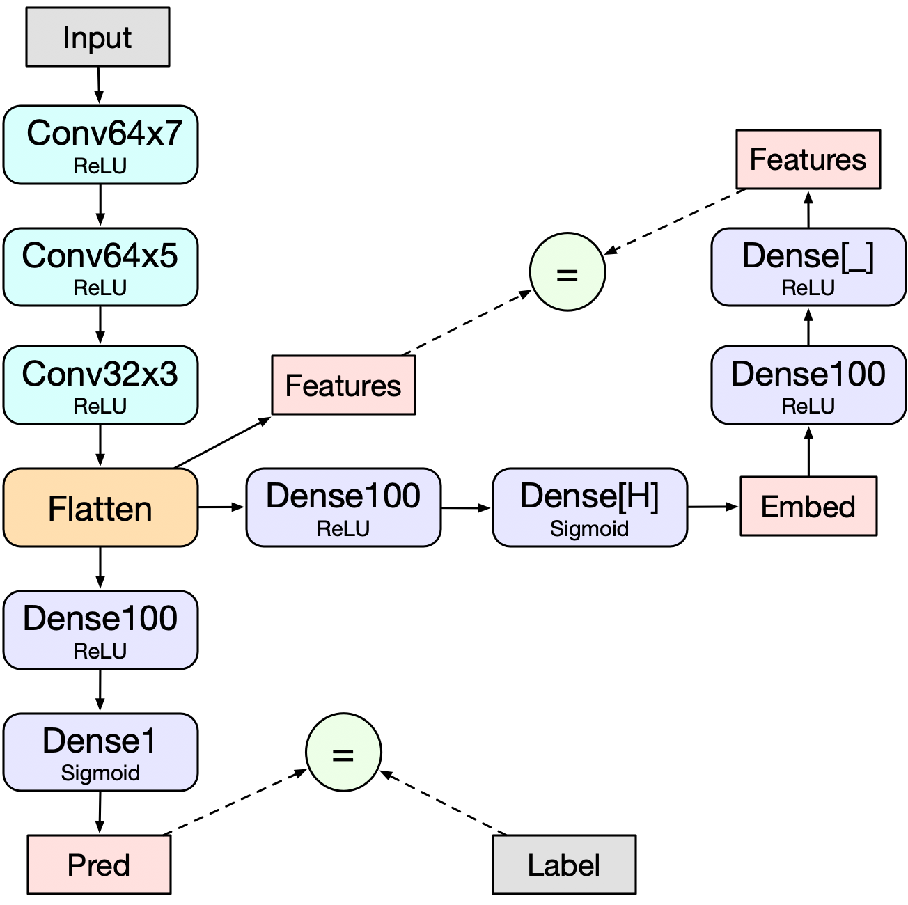
Figure 1: Model architecture for predictions and dimension $H$ embedding.

We use a deep neural network architecture as a predictive model and for embeddings (as described in 3.5). The Thompson sampling in HBBS requires priors $\mu_{0},n_{0},\alpha,\beta$ for conjugate distributions maintained at each cluster and a parameter $k$ for the number of clusters at each time step. We found HBBS was robust with respect to the prior hyperparameters, and used $\mu_{0}=0.5,n_{0}=10,\alpha=1,\beta=1$.

3.4 Baselines

One baseline method is a greedy agent that selects the batch of $M$ sequences maximizing the predictive model (Algorithm 3). We also compare against a simple exploration technique that randomly selects $\left\lceil\varepsilon M\right\rceil$ of the batch of sequences to sample, and samples the remaining $\left\lfloor(1-\varepsilon)M\right\rfloor$ of the sequences greedily (Algorithm 4).

We further analyze a batch version of GP-UCB (Algorithm 5). We first fit a Gaussian process model to the observed sequences $\mathcal{D}_{t}$ at each time step, which provides mean and uncertainty predictions $\mu,\sigma$ for each sequence in $S$. Then, we greedily sample $M$ sequences from the upper confidence bound $\mu+\sigma\sqrt{\beta}$ for a hyperparameter $\beta$. Every $m$ sequences sampled, we can refit the $\sigma$ predictions. The baseline algorithms are in Section E.

3.5 Architecture

All agents that require an embedding of prior observed sequences or a predictive model use the same architecture (Figure 1). For predictions, we fit a model to $\mathcal{D}_{t}$, the observed sequences with labels, at each time step using 1D convolutions. Further, many agents require some metric representing the similarity of different sequences, which we construct by embedding the output of the convolutional layers with an autoencoder. Since the convolutional layers extract features, the embedding will result in sequences that are similar in label for similar structural reasons clustering closely. The model has several hyperparameters (learning rate, epochs to train, embedding dimension, etc.) detailed in Appendix B, which were selected for robust performance across protein and artificial cluster environments.

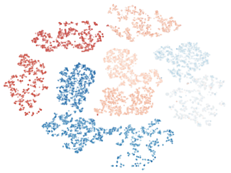
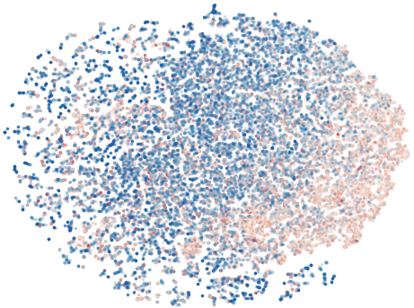
Figure 2: Cluster environment

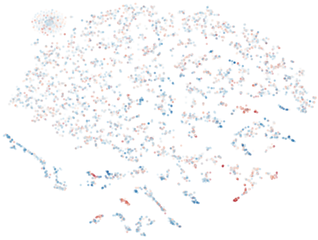
Figure 3: MPRA environment

Figure 4: BRCA1 environment

4 Experiments

4.1 Environments

We assessed our approach on one synthetic environment (ClusterEnv) as well as two real environments: one with DNA sequences (MPRA) and one with protein sequences (BRCA1). Our synthetic environment, made publicly available, simulates clusters of sequences with related features and labels with clear structure. See Appendix C for details.

4.2 Setup

We compared performance of HBBS agents against greedy, $\varepsilon$-greedy, and GP-UCB baselines on the aforementioned environments. We also generated TSNE plots (Maaten and Hinton (2008)) of the embeddings produced by our architecture when trained on half of the sequences in each environment, plotting the embedding colored by label on the other half. All agents were run for 60 time steps. The artificial environment was run with batch size $M=100$ while all of the real environments were run with $M=20$. For computational reasons, the GP-UCB algorithm could not be run on the artificial environment as doing so would require repeated GP evaluations on $\sim$3000 sequences. At the end of each run, we recorded the final Regret(0.2) obtained. For each environment, we randomly selected batches of 32 agents to run concurrently with 32 CPUs and 8 NVIDIA GeForce GTX 1080 Ti GPUs. We repeated this process until each agent had been run for 60 trials or a set amount of time had elapsed.

Due to some environments taking significantly longer to run than others, we varied this set amount between environments so there would be sufficient runs of each agent. We ran agents on the MPRA, BRCA1, and cluster environments with the aforementioned setup for approximately $50,30,20,$ and $10$ hours respectively. Final Regret(0.2) values at the last time step for each agent and environment are presented with 90% confidence intervals. We also compare the wall-clock time of agents on the MPRA environment, averaged across all trials with one representative for each class of agents with the same time complexity.

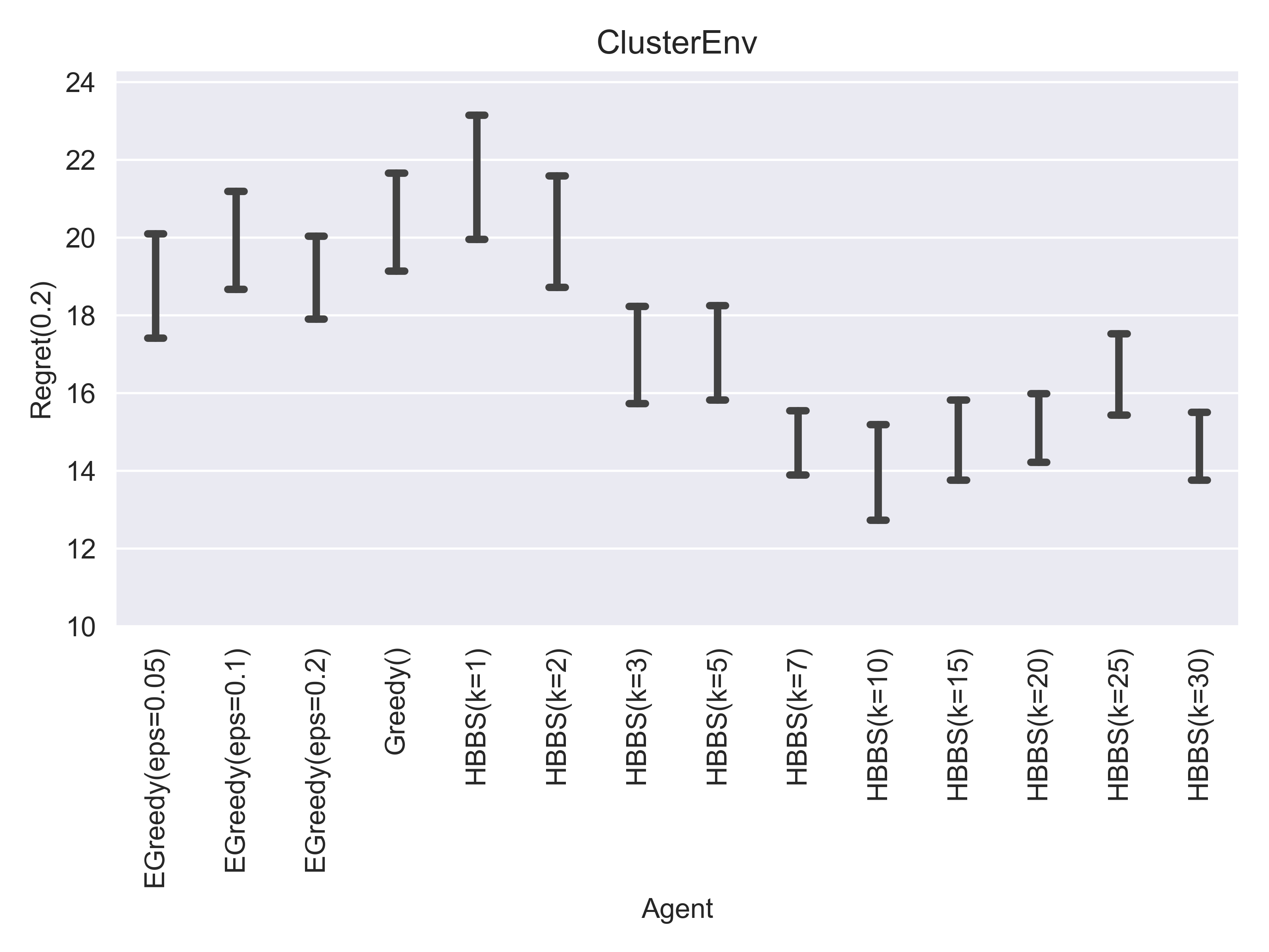
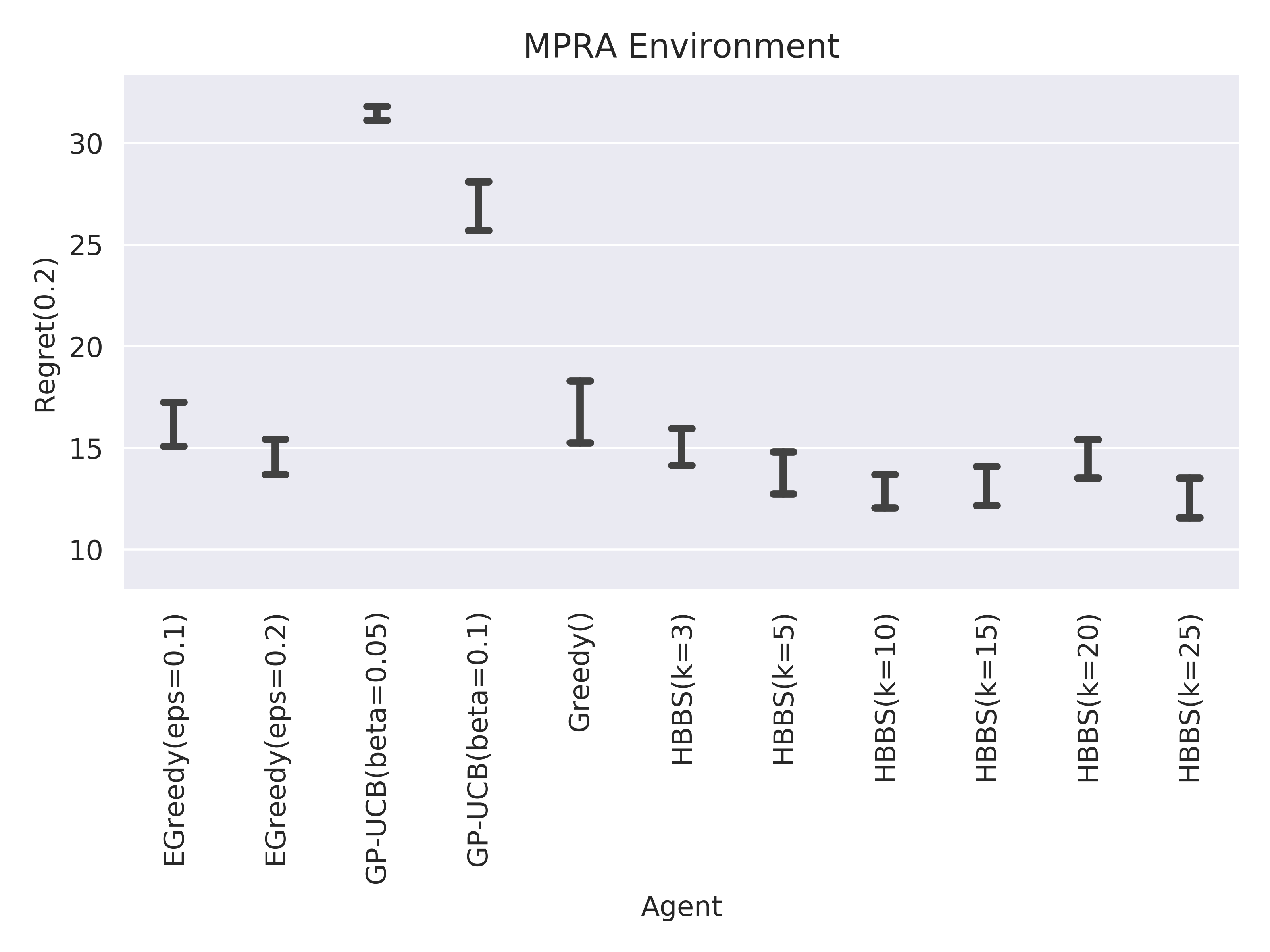
Figure 5: Cluster environment

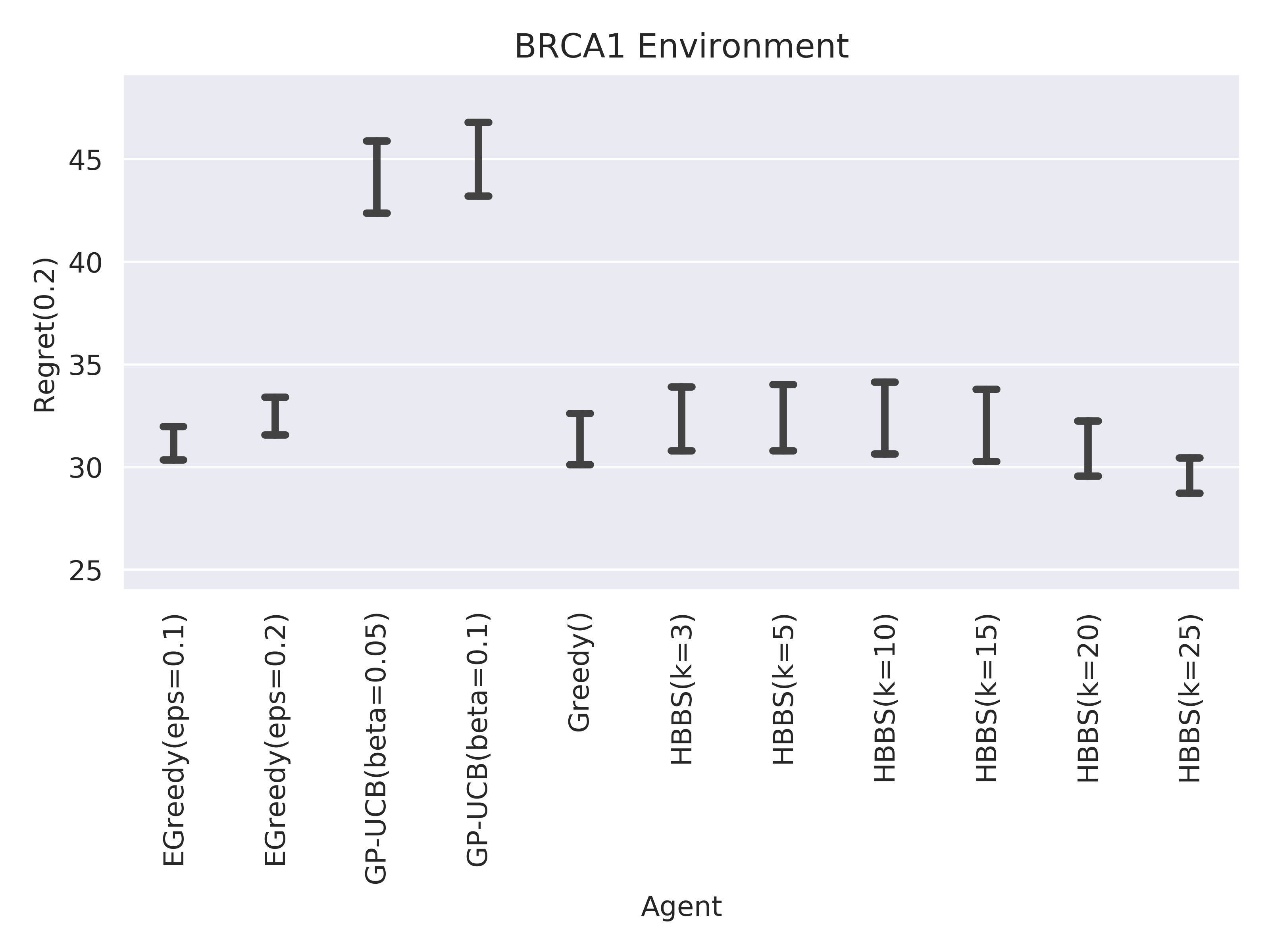
Figure 6: MPRA environment

Figure 7: BRCA1 environment

4.3 Results

We present sequence embeddings, colored by label (blue high) in Figures 4, 4, and 4. We also compare the final regret of HBBS, $\varepsilon$-greedy, and greedy agents in Figures 7, 7, and 7. See Appendix D for efficiency experiment results.

4.4 Discussion

ClusterEnv.

The clear separation of the embedding into multiple clusters indicates that HBBS may perform well on this environment.

Indeed, HBBS performs optimally near the number of actual clusters in the environment.

MPRA.

In the embedding there are multiple overlapping regions of good and bad sequences.

The HBBS agents with $k$ between $5$ and $15$, as well as $k=25$ perform best.

BRCA1.

The embedding exhibits complex structure, with numerous high scoring clusters.

The HBBS agent with $k=25$ performs statistically significantly better than all other agents.

5 Conclusion

We found HBBS to perform the best on all the environments presented with obvious nonlinear structure to their embedding—its primary shortcoming in performance is often achieving similar or slightly improved results to $\varepsilon$-greedy. The overall trends we observe in wall-clock time demonstrate HBBS can effectively search across tens of thousands of sequences with easy scalability to larger datasets. $\varepsilon$-greedy has been documented as a reliable baseline for similar active search tasks, though its performance is highly dependent on the parameter $\varepsilon$ (Hernández-Lobato et al. (2017)). Most surprising is the relatively poor performance of GPs, but this can be explained by our observation that methods that can take advantage of the neural network’s predictive capacity consistently outperform those that do not.

In execution time, HBBS can cause methods which are superlinear in time-complexity with respect to the number of sequences in the dataset to run faster. For instance, if HBBS is used with GP-UCB within each partition, by making the partitions arbitrarily small, the $\mathcal{O}(n^{3})$ time complexity of GP-UCB can be mitigated. This key insight that HBBS is a general framework that can improve speed or performance and can be used hierarchically with any method per partition allows its extension to both increasingly large datasets and increasingly specialized search methods.

Acknowledgments

We would like to acknowledge support for this project from the Stanford CURIS program, the Schmidt Science Fellowship program, and Emma Brunskill and lab members. Thank you to the Google Cloud Platform for supplying research credits for this work.

A Code

Our Gym environment and our code for all experiments is publicly available at
https://github.com/StanfordAI4HI/HBBS.

B Model Details

We use a learning rate of $\alpha=5\cdot 10^{-4}$ with MSE loss at each of the green nodes in Figure 1 for both the autoencoder and prediction portions of the model, and a minibatch size of $100$. We also use an embedding dimension of $H=5$.

The gray nodes in Figure 1 represent inputs and the red nodes represent output. Input values are one-hot encoded sequences.

C Environments

Algorithm 2 ClusterEnv[$N,n,\sigma,c,\ell$]

1:procedure Generate

2:  $\triangleright$ Produces sequences $S$ labeled by $f$

3:     $S\leftarrow\{\}$

4:     for $i\in\{1\ldots N\}$ do

5:         $\mu\sim U(\frac{-1}{2},\frac{1}{2})$

6:         $\xi\sim\sigma U(0,1)$

7:         for $j\in\{1\ldots\ell\}$ do

8:              $x_{1},x_{2},x_{3},x_{4}\sim\mathcal{N}(0,1)$

9:              $v_{j}\leftarrow[|x_{1}|^{1/c},|x_{2}|^{1/c},|x_{3}|^{1/c},|x_{4}|^{1/c}]$

10:              $v_{j}\leftarrow v_{j}/\sum_{i}|x_{i}|^{1/c}$

11:         end for

12:         $u\leftarrow$ distribution over $\{A,C,T,G\}^{\ell}$

13:      with each component one of the $v_{j}$

14:         for $j\in\{1\ldots n\}$ do

15:              $s\sim u$

16:              $S\leftarrow S\cup\{s\}$

17:              $y\sim\mathcal{N}(\mu,\xi)$

18:              $f(s)\leftarrow\frac{1}{1+e^{-y}}$

19:         end for

20:     end for

21:end procedure

C.1 ClusterEnv Synthetic Environment

We present a simple artificial environment that mimics the traditional bandit setting with artificial DNA sequences. This environment consists of a set of sequences $\{A,T,C,G\}^{\ell}$ in $N$ clusters each containing $n$ sequences. Each cluster is generated by first selecting a probability mass function over $\{A,T,C,G\}^{\ell}$ as well as a Gaussian label distribution, then sampling $n$ sequences (Algorithm 2). To ensure labels are within $[0,1]$, they are clamped with the sigmoid function. Because labels depend only on the cluster of a sequence, each cluster can be viewed as an arm in a bandit problem, with a reward distribution determined by the labels it contains. Since the distributions are Gaussian, an optimal agent for Gaussian bandits with $N$ arms will also perform well on ClusterEnv if it views the clusters as the $N$ arms. We used the parameters $N=10,n=30000,\sigma=0.1,c=0.2$ for our experiments as this setup yielded a small number of clusters with highly distinct structure and reward distribution.

C.2 Real Environments

We also evaluate the agents described in Section 3 on real biological sequence environments.

DNA Sequences.

DNA environments consist of sequences of the form $\{A,C,T,G\}^{l}$, with an optional additional strand direction identifier, $+$ or $-$. We test on Massively Parallel Reporter Assay (MPRA) sequences of length 150 base pairs (Urtecho et al. (2020)) designed to promote gene expression to higher levels. The MPRA dataset has exponentially distributed scores, so to avoid creating an environment putting undue focus on any particular sequences, we renormalize it to have labels uniformly distributed on $[0,1].$

Protein Sequences.

Protein sequence environments consist of sequences of 20 different amino acids of the same length representing mutated versions of a protein, along with labels corresponding to the effects of their mutations on their function. We focus on the the protein BRCA1 in this paper by evaluating data from a parallel assay to measure the effects of missense substitutions in the RING domain of BRCA1 on its activity and binding functions (Starita et al. (2015)).

D Efficiency

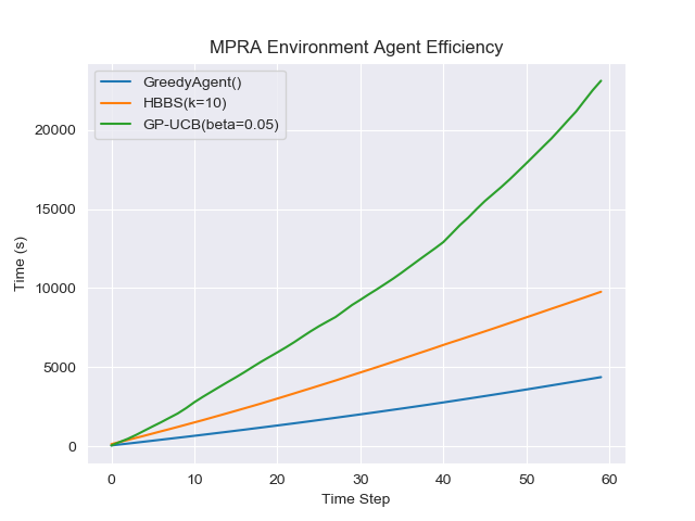
Figure 8: Total wall-clock time used at each timestep.

Discussion.

Using HBBS adds overhead which is linear with respect to time step. GP-UCB achieves by far the worst performance, especially at larger time steps. This performance is consistent with the $\mathcal{O}(n^{3})$ GP-fitting step which GP-UCB must perform multiple times per action.

E Baseline Algorithms

Algorithm 3 Greedy

1:procedure Act($f,\mathcal{D},M,S$)

2:  $\triangleright$ Observations $\mathcal{D}$, labels $f$; select $M$ sequences in $S$ to sample.

3:     Fit predictor $\hat{f}$ to $f,\mathcal{D}$

4:     $A\leftarrow\{\}$

5:     for $i\in\{1\ldots M\}$ do

6:         $a\leftarrow\underset{x\in(S\setminus(\mathcal{D}\cup A))}{\arg\max}\hat{f}(x)$

7:         $A\leftarrow A\cup\{a\}$

8:     end for

9:     select $A$

10:end procedure

Algorithm 4 $\varepsilon$-Greedy[$\varepsilon$]

1:procedure Act($f,\mathcal{D},M,S$)

2:  $\triangleright$ Observations $\mathcal{D}$, labels $f$; select $M$ sequences in $S$ to sample.

3:     Fit predictor $\hat{f}$ to $f,\mathcal{D}$

4:     $A\leftarrow$ random sample of $\lceil\varepsilon M\rceil$ sequences in $S-\mathcal{D}$

5:     for $i\in\{1\ldots\lfloor(1-\varepsilon)M\rfloor\}$ do

6:         $a\leftarrow\underset{x\in(S\setminus(\mathcal{D}\cup A))}{\arg\max}\hat{f}(x)$

7:         $A\leftarrow A\cup\{a\}$

8:     end for

9:     select $A$

10:end procedure

Algorithm 5 GP-UCB[$\beta,m$]

1:procedure Act($f,\mathcal{D},M,S$)

2:  $\triangleright$ Observations $\mathcal{D}$, labels $f$; select $M$ sequences in $S$ to sample.

3:     Fit embedding to $f,\mathcal{D}$, use to fit GP $\mu,\sigma$ to $f,\mathcal{D}$

4:     $A\leftarrow\{\}$

5:     for $i\in\{1\ldots M\}$ do

6:         $a\leftarrow\underset{x\in(S\setminus(\mathcal{D}\cup A))}{\arg\max}\mu(x)+\sigma(x)\sqrt{\beta}$

7:         $A\leftarrow A\cup\{a\}$

8:         if $m$ divides $i$ then

9:              Refit $\sigma$ with $\mathcal{D}\cup A$

10:         end if

11:     end for

12:     select $A$

13:end procedure

References

- Alley et al. (2019) Ethan C Alley, Grigory Khimulya, Surojit Biswas, Mohammed AlQuraishi, and George M Church. Unified rational protein engineering with sequence-based deep representation learning. Nature methods, 16(12):1315–1322, 2019.
- Biswas et al. (2018) Surojit Biswas, Gleb Kuznetsov, Pierce J Ogden, Nicholas J Conway, Ryan P Adams, and George M Church. Toward machine-guided design of proteins. bioRxiv, page 337154, 2018.
- Brockman et al. (2016) Greg Brockman, Vicki Cheung, Ludwig Pettersson, Jonas Schneider, John Schulman, Jie Tang, and Wojciech Zaremba. Openai gym. arXiv preprint arXiv:1606.01540, 2016.
- Brookes and Listgarten (2018) David H Brookes and Jennifer Listgarten. Design by adaptive sampling. arXiv preprint arXiv:1810.03714, 2018.
- Damianou and Lawrence (2013) Andreas Damianou and Neil Lawrence. Deep gaussian processes. In Artificial Intelligence and Statistics, pages 207–215, 2013.
- Desautels et al. (2014) Thomas Desautels, Andreas Krause, and Joel W Burdick. Parallelizing exploration-exploitation tradeoffs in gaussian process bandit optimization. The Journal of Machine Learning Research, 15(1):3873–3923, 2014.
- Gardner et al. (2018) Jacob Gardner, Geoff Pleiss, Kilian Q Weinberger, David Bindel, and Andrew G Wilson. Gpytorch: Blackbox matrix-matrix gaussian process inference with gpu acceleration. In Advances in Neural Information Processing Systems, pages 7576–7586, 2018.
- Gómez-Bombarelli et al. (2018) Rafael Gómez-Bombarelli, Jennifer N Wei, David Duvenaud, José Miguel Hernández-Lobato, Benjamín Sánchez-Lengeling, Dennis Sheberla, Jorge Aguilera-Iparraguirre, Timothy D Hirzel, Ryan P Adams, and Alán Aspuru-Guzik. Automatic chemical design using a data-driven continuous representation of molecules. ACS central science, 4(2):268–276, 2018.
- González et al. (2016) Javier González, Zhenwen Dai, Philipp Hennig, and Neil Lawrence. Batch bayesian optimization via local penalization. In Artificial intelligence and statistics, pages 648–657, 2016.
- Gupta and Zou (2019) Anvita Gupta and James Zou. Feedback gan for dna optimizes protein functions. Nature Machine Intelligence, 1(2):105–111, 2019.
- Hernández-Lobato et al. (2017) José Miguel Hernández-Lobato, James Requeima, Edward O Pyzer-Knapp, and Alán Aspuru-Guzik. Parallel and distributed thompson sampling for large-scale accelerated exploration of chemical space. In Proceedings of the 34th International Conference on Machine Learning-Volume 70, pages 1470–1479. JMLR. org, 2017.
- Kathuria et al. (2016) Tarun Kathuria, Amit Deshpande, and Pushmeet Kohli. Batched gaussian process bandit optimization via determinantal point processes. In Advances in Neural Information Processing Systems, pages 4206–4214, 2016.
- Killoran et al. (2017) Nathan Killoran, Leo J. Lee, Andrew Delong, David Duvenaud, and Brendan J. Frey. Generating and designing dna with deep generative models, 2017.
- Maaten and Hinton (2008) Laurens van der Maaten and Geoffrey Hinton. Visualizing data using t-sne. Journal of machine learning research, 9(Nov):2579–2605, 2008.
- McIntire et al. (2016) Mitchell McIntire, Daniel Ratner, and Stefano Ermon. Sparse gaussian processes for bayesian optimization. In UAI, 2016.
- Snoek et al. (2015) Jasper Snoek, Oren Rippel, Kevin Swersky, Ryan Kiros, Nadathur Satish, Narayanan Sundaram, Mostofa Patwary, Mr Prabhat, and Ryan Adams. Scalable bayesian optimization using deep neural networks. In International conference on machine learning, pages 2171–2180, 2015.
- Starita et al. (2015) Lea M Starita, David L Young, Muhtadi Islam, Jacob O Kitzman, Justin Gullingsrud, Ronald J Hause, Douglas M Fowler, Jeffrey D Parvin, Jay Shendure, and Stanley Fields. Massively parallel functional analysis of brca1 ring domain variants. Genetics, 200(2):413–422, 2015.
- Thompson (1933) William R Thompson. On the likelihood that one unknown probability exceeds another in view of the evidence of two samples. Biometrika, 25(3/4):285–294, 1933.
- Urtecho et al. (2020) Guillaume Urtecho, Kimberly D. Insigne, Arielle D. Tripp, Marcia Brinck, Nathan B. Lubock, Hwangbeom Kim, Tracey Chan, and Sriram Kosuri. Genome-wide functional characterization of escherichia coli promoters and regulatory elements responsible for their function. bioRxiv, 2020. doi: 10.1101/2020.01.04.894907. URL https://www.biorxiv.org/content/early/2020/01/06/2020.01.04.894907.
- Wang et al. (2017) Zi Wang, Clement Gehring, Pushmeet Kohli, and Stefanie Jegelka. Batched large-scale bayesian optimization in high-dimensional spaces. arXiv preprint arXiv:1706.01445, 2017.
- Yang et al. (2019) Kevin K Yang, Zachary Wu, and Frances H Arnold. Machine-learning-guided directed evolution for protein engineering. Nature methods, 16(8):687–694, 2019.