Abstract

A method of regulating spin dynamics of the so-called magnetic graphene is analyzed. Magnetic moments can be incorporated into graphene flakes and graphene ribbons through defects, such as adatoms and vacancies. Local spins can also be attached to graphene at hydrogenated zigzag edges. Spin flips can be produced by transverse pulses and by connecting the sample to a resonance electric coil. The action of the resonator feedback field strongly accelerates spin reversal. The possibility of fast spin reversal is important for spintronics and for quantum information processing allowing for an efficient functioning of spin registers.

Keywords: Spin dynamics; graphene flakes; magnetic defects; magnetization reversal

1 Traditional approaches

Graphene is an allotrope of carbon in the form of a sheet of a single layer (monolayer) of carbon atoms, tightly bound in a hexagonal honeycomb lattice with a molecular bond length of $0.142$ nanometers. The properties of graphene have been described in detail in several reviews [1, 2, 3, 4, 5, 6, 7, 8, 9] discussing a number of applications within different scientific disciplines, e.g., in high-frequency electronics, bio sensors, chemical sensors, magnetic sensors, ultra-wide bandwidth photodetectors, energy storage and generation.

The so-called magnetic graphene can be created by incorporating local defects, such as adatoms and vacancies, into graphene flakes and ribbons [10, 11, 12, 13]. This can be done in different ways, for instance, by irradiating graphene flakes or using mechanical and chemical methods of incorporating defects. Local magnetic moments can be attached to graphene flakes at hydrogenated zigzag edges, forming a kind of nanomolecules exhibiting ferromagnetism at room temperatures. The hydrogenated zigzag-edge groups can possess local magnetic moments with spins $1/2$, $3/2$, and $5/2$.

It is the magnetic properties of graphene that is the topic of the present chapter. More precisely, our aim is to describe how the direction of magnetic moments could be regulated. The possibility of regulating the polarization of spins is of principal importance for spintronics as well as for information processing.

The most often used method of realizing spin reversal is by acting on polarized spins by an alternating transverse magnetic field. For the efficient spin reversal, it is necessary to find the appropriate strength of the alternating field, its frequency, and duration. Below we describe another method in which the required field, with the necessary features, is created automatically, being a feedback field.

2 Magnetic defects coupled to a resonance electric circuit

Magnetic defects in graphene interact through exchange forces, which can be characterized [10, 11, 12, 13] by the anisotropic Heisenberg model

$$\hat{H}_{def}=-\;\frac{1}{2}\sum_{i\neq j}J_{ij}\left[\left(S_{i}^{x}S_{j}^{x}+S_{i}^{y}S_{j}^{y}\right)+\alpha S_{i}^{z}S_{j}^{z}\right]\;,$$ (1)

in which $S_{i}^{\nu}$ is a $\nu$ spin component of the $i$-th magnetic defect, $J_{ij}$ is the exchange interaction potential, and $\alpha$ is an anisotropy parameter. The index $i=1,2,\ldots,N$ enumerates the sites of magnetic defects. The typical values of the exchange interactions for the nearest neighbors are $J_{ij}<0.1$ eV, that is $J_{ij}<10^{-13}$ erg. Hence $J_{ij}/\hbar<10^{14}$ s^-1. The magnetic anisotropy usually is not large, such that $\alpha$ is close to one.

Adding the Zeeman part gives us the total Hamiltonian

$$\hat{H}=\hat{H}_{def}-\mu_{S}\sum_{j=1}^{N}{\bf B}\cdot{\bf S}_{j}\;,$$ (2)

where $\mu_{S}$ is the magnetic moment of a defect with spin $S$. The external magnetic field consists of two terms,

$${\bf B}=B_{0}{\bf n}_{z}+H{\bf n}_{x}\;.$$ (3)

One term is a constant magnetic field $B_{0}$ along a unit vector ${\bf n}_{z}$. In addition, the sample is assumed to be inserted into a magnetic coil of an electric circuit, so that moving spins induce electric current in the circuit, which creates a magnetic feedback field $H$. With the coil axis along the unit vector ${\bf n}_{x}$, the feedback field acts along ${\bf n}_{x}$.

The electric circuit contains resistance $R$, inductance $L$, and capacity $C$. The coil has $n$ turns, length $l$, and cross-sectional area $A_{coil}$, hence volume $V_{coil}=A_{coil}l$. The induced current is given by the Kirchhoff equation

$$L\;\frac{dj}{dt}+Rj+\frac{1}{C}\int_{0}^{t}j(t^{\prime})\;dt^{\prime}=-\;\frac{d\Phi}{dt}\;,$$ (4)

in which $\Phi$ is the magnetic flux

$$\Phi=\frac{4\pi}{c}\;nA_{coil}\eta m_{x}\;,$$ (5)

where $\eta\approx V/V_{coil}$ is the filling factor, and $V$ is the sample volume. The magnetic flux is formed by the $x$ component of the moving magnetization density

$$m_{x}=\frac{\mu_{s}}{V}\sum_{j=1}^{N}\;\langle\;S_{j}^{x}\;\rangle\;.$$ (6)

The induced electric current, circulating over the coil, creates a magnetic field

$$H\equiv\frac{4\pi n}{cl}\;j\;.$$ (7)

The circuit natural frequency is given by the expression

$$\omega\equiv\frac{1}{\sqrt{LC}}\qquad\left(L\equiv 4\pi\;\frac{n^{2}A_{coil}}{c^{2}l}\right)\;$$ (8)

and the circuit damping by

$$\gamma\equiv\frac{R}{2L}=\frac{\omega}{2Q}\;,$$ (9)

with $Q$ being the quality factor

$$Q\equiv\frac{\omega L}{R}=\frac{\omega}{2\gamma}\;.$$ (10)

Then from the Kirchhoff equation for the induced electric current, we get [14] the equation for the feedback magnetic field

$$\frac{dH}{dt}+2\gamma H+\omega^{2}\int_{0}^{t}H(t^{\prime})\;dt^{\prime}=-4\pi\eta\;\frac{dm_{x}}{dt}\;.$$ (11)

Finally, introducing the dimensionless feedback field

$$h\equiv\frac{H}{B_{0}}$$ (12)

and differentiating equation (11), we come to the equation

$$\frac{d^{2}h}{dt^{2}}+\frac{1}{Q}\;\frac{dh}{dt}+h=4\pi\beta\;\frac{d^{2}e_{x}}{dt^{2}}\;,$$ (13)

in which the parameter

$$\beta=\left|\;\frac{\mu_{S}SN}{B_{0}V_{coil}}\right|$$ (14)

characterizes the strength of coupling of the sample with the circuit. The electromotive force in the right-hand side of equation (13) is formed by moving spins

$$e_{\nu j}=\frac{1}{S}\;\langle\;S_{j}^{\nu}\;\rangle\qquad(\nu=x,y,z)\;,$$ (15)

with

$$e_{\nu}=\frac{1}{N}\sum_{j=1}^{N}e_{\nu j}=\frac{1}{NS}\sum_{j=1}^{N}\;\langle\;S_{j}^{\nu}\;\rangle$$ (16)

being the average over the sample $\nu$-th spin component.

Note that $j$ is the total electric current in the circuit generated by all spins inside the coil. This is why the expression for the electromotive force contains the summation over all spins. Respectively, the feedback magnetic field $H$, proportional to the total electric current $j$, is the field resulting from the summary action of all spins, independently from their location inside the coil. In practice, the distribution of magnetic defects can be arbitrary and we do not require any translational invariance. And really we consider the case, when the defects are located at the graphene sample edges. Their location does not change the total current induced in the coil, but does influence the equations of motion and, respectively, the overall dynamics. The equations of motion, treated in the following section, study the case of magnetic defects located at the edges of graphene flakes.

Angle brackets imply statistical averaging

$$\langle\;S_{j}^{\alpha}\;\rangle={\rm Tr}\hat{\rho}(0)S_{j}^{\alpha}(t)=\langle\;S_{j}^{\alpha}(t)\;\rangle\;,$$ (17)

in which $\hat{\rho}(0)$ is the statistical operator at the initial time $t=0$. As far as the system is nonequilibrium, the standard notion of temperature, strictly speaking, is not defined. In principle, for nonequilibrium spins, it could be possible to introduce a negative effective spin temperature dependent on time [15]. This, however, is not necessary, since the time evolution of average spins is prescribed by the Heisenberg equations of motion. And all information on the initial statistical operator can be included in the initial values

$$e_{\alpha}(0)=\frac{1}{NS}\sum_{j=1}^{N}\langle\;S_{j}^{\alpha}(0)\;\rangle=\frac{1}{NS}\sum_{j=1}^{N}{\rm Tr}\hat{\rho}(0)S_{j}^{\alpha}(0)\;,$$ (18)

where the left-hand side is given as an initial condition.

The initial conditions to equation (13) are

$$h(0)=\dot{h}(0)=0\;,$$ (19)

where the overdot signifies time derivative. The electric circuit is tuned in resonance with the Zeeman frequency,

$$\omega_{0}=\frac{1}{\hbar}\;|\;\mu_{S}B_{0}\;|\;,$$ (20)

so that

$$\omega=\omega_{0}\;,$$ (21)

because of which the electric circuit is termed a resonance circuit.

Magnetic defects are assumed to be incorporated into a graphene flake that is in equilibrium, hence being characterized by temperature. Generally speaking, the interaction of magnetic defects with the graphene matrix can result in the appearance of temperature effects in spin motion. The main influence of these effects is in the arising attenuation in spin dynamics caused by the interaction of spins with phonon fluctuations. This leads to the emergence of the so-called attenuation term $\gamma_{1}=1/T_{1}$ in the equations of spin motion [15] that is of the order of the strength of spin-phonon interactions and depending on temperature. However, considering short-time spin dynamics, the term $\gamma_{1}$ can be safely omitted. This is because fast coherent spin reversal, as is studied in the present paper, occurs during the time shorter than the time of spin dephasing $T_{2}$ being of the order of the strength of spin interactions. Spin-phonon interactions are practically always much smaller than spin interactions, so that $T_{2}\ll T_{1}$. This means that if the main processes occur at times shorter than $T_{2}$, and $\gamma_{1}\ll\gamma_{2}$, then the attenuation $\gamma_{1}=1/T_{1}$ can be neglected. So, the dependence of $\gamma_{1}$ on temperature is of no importance. Of course, the said above assumes that temperature is not too high, being such that $k_{B}T/J_{ij}\ll 1$. Under this condition, spin dynamics is much more influenced by spin interactions, but not by temperature effects. If the nearest-neighbor spin interactions are of order $J_{ij}\sim 10^{-13}$ erg, as is mentioned at the beginning of this section, this means that temperature is considered as low for $T\ll 10^{3}$ K. Throughout the paper, we keep in mind that graphene temperature is low in the above sense, so that temperature effects are negligible.

3 Equations of motion for spin variables

We write the equations for the spin variables (15) using the Heisenberg equations of motion

$$i\hbar\;\frac{de_{\nu j}}{dt}=\frac{1}{S}\;\langle\;[\;S_{j}^{\nu},\;\hat{H}\;]\;\rangle$$ (22)

and then calculate the time dependence of variable (16) employing the mean-field approximation

$$\langle\;S_{i}^{\mu}S_{j}^{\nu}\;\rangle=\langle\;S_{i}^{\mu}\;\rangle\langle\;S_{j}^{\nu}\;\rangle\;.$$ (23)

At the initial moment of time, spins are polarized along the axis $z$ so that the distribution of up or down spins at their sites is random, but their average polarization (16) is fixed as

$$\langle\;e_{z}(0)\;\rangle=-0.9\;.$$ (24)

The external magnetic field $B_{0}$ is directed so that the initial spin polarization (24) corresponds to a nonequilibrium state, while the equilibrium spin polarization would correspond to the up direction. Our aim is to find the system parameters that could produce fast spin reversal, when the reversal time, that is, the time from the starting point to the moment of time, where the average spin is reversed, would be short. Also, it is desirable that the reversal be practically complete and after the reversal the average spin would not strongly fluctuate. Such a regime of spin reversal is optimal for applications in spintronics and information processing.

4 Defects at zigzag edges of graphene flakes

As a concrete system, we consider magnetic defects caused by hydrogenation of zigzag edges of graphene flakes. Spins interact through the nearest neighbors, with a ferromagnetic exchange potential $J>0$. For simplicity, the value of the external field $B_{0}$ is taken such that $JS=\hbar\omega_{0}$. We study the dynamics of spin reversals by varying the anisotropy parameter $\alpha$, coupling parameter $\beta$, and the resonator quality factor $Q$. We pay attention to the following three features: (i) when the reversal time is shorter, (ii) if the reversal is complete, and (iii) if there appear spin oscillations after the reversal.

In Fig. 1, there is no anisotropy, hence $\alpha=1$, and the coupling parameter is set to $\beta=0.1$, while the quality factor is varied. The temporal behavior of the spin polarization $e_{z}$ as a function of time in units of $1/\omega$ is shown. The larger the quality factor $Q$, the shorter the reversal time. The reversal is complete, but there appear oscillations after the reversal, if $Q>1$.

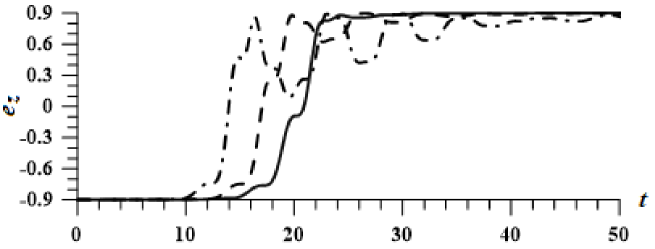
Figure 1: Longitudinal, $e_{z}$, spin polarization as a function of dimensionless time (measured in units of $1/\omega$), for the coupling parameter $\beta=0.1$ and anisotropy parameter $\alpha=1$ (no anisotropy) for different resonator quality factors $Q$: (a) $Q=1$ (solid line), (b) $Q=2$ (dashed line), and (c) $Q=5$ (dashed-dotted line).

The anisotropy is also absent in Fig. 2, where $\alpha=1$. The coupling parameter is smaller than in the previous figure, being $\beta=0.01$. The smaller coupling parameter makes the reversal time longer. The reversal is complete. The after-reversal oscillations are practically absent even for $Q=5$.

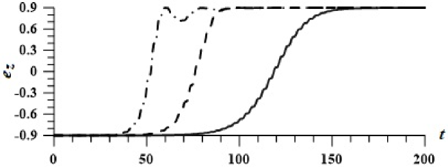
Figure 2: Longitudinal, $e_{z}$, spin polarization as a function of dimensionless time (measured in units of $1/\omega$), for the coupling parameter $\beta=0.01$ and anisotropy parameter $\alpha=1$ (no anisotropy) for different resonator quality factors $Q$: (a) $Q=1$ (solid line), (b) $Q=2$ (dashed line), and (c) $Q=5$ (dashed-dotted line).

Figure 3 studies the influence of the anisotropy, under the fixed coupling parameter $\beta=0.01$ and the quality factor $Q=1$. As is expected, the larger the anisotropy, the longer the reversal time. The parasitic oscillations are absent, but the reversal is not complete, when the anisotropy parameter $\alpha>1.5$.

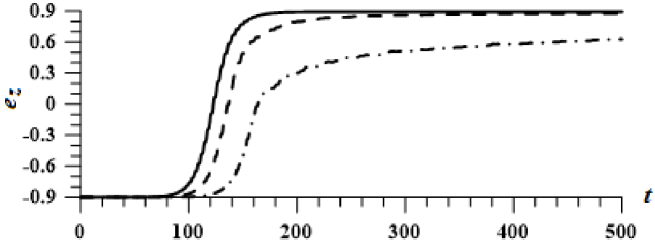
Figure 3: Longitudinal, $e_{z}$, spin polarization as a function of dimensionless time (measured in units of $1/\omega$), for the coupling parameter $\beta=0.01$ and the resonator quality factor $Q=1$ for different anisotropy parameters $\alpha$: (a) $\alpha=1.2$ (solid line), (b) $\alpha=1.4$ (dashed line), and (c) $\alpha=1.6$ (dashed-dotted line).

In Fig. 4, the role of the coupling parameter is explored, under the given $\alpha=1$ and $Q=1$. Increasing $\beta$ diminishes the reversal time. Slight oscillations occur for $\beta>0.2$.

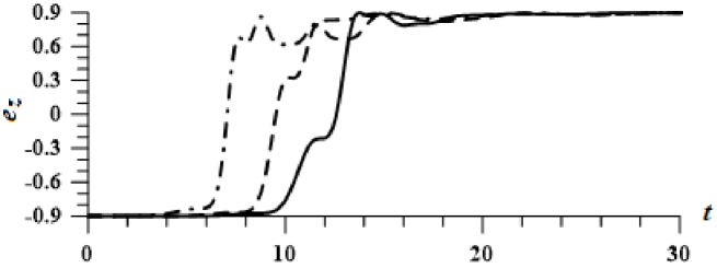
Figure 4: Longitudinal, $e_{z}$, spin polarization as a function of dimensionless time (measured in units of $1/\omega$), for the resonator quality factor $Q=1$ and anisotropy parameter $\alpha=1$, for different coupling parameters $\beta$: (a) $\beta=0.2$ (solid line), (b) $\beta=0.3$ (dashed line), and (c) $\beta=0.4$ (dashed-dotted line).

Figure 5 demonstrates that increasing the quality factor, under $\alpha=1$ and the larger coupling parameter $\beta=0.4$, shortens the reversal time, although rather strong oscillations arise for $Q>1$.

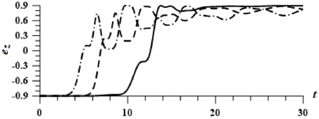
Figure 5: Longitudinal, $e_{z}$, spin polarization as a function of dimensionless time (measured in units of $1/\omega$), for the coupling parameter $\beta=0.4$ and anisotropy parameter $\alpha=1$ for different resonator quality factors $Q$: (a) $Q=1$ (solid line), (b) $Q=2$ (dashed line), and (c) $Q=3$ (dashed-dotted line).

For sufficiently large coupling parameter, such as in Fig. 6, where $\beta=0.2$, the reversal time does not essentially depends on the anisotropy, however under strong anisotropy $\alpha>1.5$ the reversal is never complete.

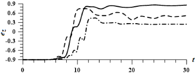
Figure 6: Longitudinal, $e_{z}$, spin polarization as a function of dimensionless time (measured in units of $1/\omega$), for the coupling parameter $\beta=0.2$ and the resonator quality factor $Q=1$, for different anisotropy parameters $\alpha$: (a) $\alpha=1.5$ (solid line), (b) $\alpha=3$ (dashed line), (c) $\alpha=5$ (dashed-dotted line).

In that way, to realize optimal conditions for spin reversal, requiring the validity of three criteria, short reversal time, complete spin reversal, and the absence of parasitic oscillations, one has to appropriately adjust the system parameters $\alpha$, $\beta$, and $Q$. From numerical calculations, we find for the product of these parameters the condition $\alpha\beta Q\sim 0.1$, when all three criteria are satisfied. Keeping in mind the definition of $\beta$ and $Q$, we come to the condition

$$\frac{\rho\mu_{S}^{2}S}{\hbar\gamma}\sim 0.1\;,$$ (25)

where $\rho$ is the density of magnetic defects. In this way, for realizing optimal spin reversal in graphene flakes, one needs to choose the system parameters satisfying estimate (25).

5 Conclusion

We have described a method of regulating spin dynamics of the so-called magnetic graphene. Magnetic moments can be incorporated into graphene flakes and graphene ribbons through defects, such as adatoms and vacancies. Also, spins can be located at hydrogenated zigzag edges of graphene. Spin reversal can be produced by connecting the sample to a resonance electric circuit. The action of the resonator feedback field strongly accelerates spin reversal. This method is essentially simpler than spin reversal by means of transverse alternating fields, where one needs to define the field amplitude, its frequency, and duration. The feedback field adjusts automatically, being created by moving spins themselves. Choosing the needed parameters, one can easily regulate the spin reversal time, finding the conditions when there are no after-reversal oscillations. The described method of fast and easily regulated spin reversal can find applications in spintronics and in quantum information processing. Other applications can be connected with the electromagnetic radiation emitted by coherently moving spins [14], as it is generated in different systems under coherent spin motion [16, 17, 18, 19, 20, 21, 22]. It is important to stress that the coherent spin motion, when no strong external coherent fields are involved, necessarily requires the presence of a resonator [23].

References

- [1] A.H. Castro Neto, F. Guinea, N.M. Peres, K.S. Novoselov, and A.K. Geim. The electronic properties of graphene. Rev. Mod. Phys., 81: 109–162, 2009.
- [2] D.S. Abergel, V. Apalkov, J. Berashevich, K. Ziegler, and T. Chakraborty. Properties of graphene: a theoretical perspective. Adv. Phys., 59: 261–482, 2010.
- [3] M.S. Dresselhaus, A. Jorio, R. Saito. Characterizing graphene, graphite, and carbon nanotubes by Raman spectroscopy. Annu. Rev. Condens. Matter Phys., 1: 89–108, 2010.
- [4] S. Das Sarma, S. Adam, E.H. Hwang, and E. Rossi. Electronic transport in two-dimensional graphene. Rev. Mod. Phys., 83: 407–470, 2011.
- [5] M.O. Goerbig. Electronic properties of graphene in a strong magnetic field. Rev. Mod. Phys., 83: 1193–1244, 2011.
- [6] R. Saito, M. Hofman, G. Dresselhaus, A. Jorio, and M.S. Dresselhaus. Raman spectroscopy of graphene and carbon nanotubes. Adv. Phys., 60: 413–550, 2011.
- [7] V.N. Kotov, B. Uchoa, V.M. Pereira, F. Guinea, and A.H. Castro Neto. Electron–electron interactions in graphene: current status and perspectives. Rev. Mod. Phys., 84: 1067–1126, 2012.
- [8] E. McCann and M. Koshiro. The electronic properties of bilayer graphene. Rep. Prog. Phys., 76: 056503, 2013.
- [9] T.O. Wehling, A.M. Black–Schaffer, and A.V. Balatsky. Dirac materials. Adv. Phys., 63: 1–76, 2014.
- [10] O.V. Yaziev. Emergence of magnetism in graphene materials and nanostructures. Rep. Prog. Phys., 73: 056501, 2010.
- [11] J.J. Palacios, J. Fernandez-Rossier, L. Brey, and H.A. Fertig. Electronic and magnetic structure of graphene nanoribbons. Semicond. Sci. Technol., 25: 033003, 2010.
- [12] M.I. Katsnelson. Graphene: Carbon in Two Dimensions. Cambridge University, Cambridge, 2012.
- [13] T. Enoki and T. Ando. Physics and Chemistry of Graphene. Pan Stanford, Singapore, 2013.
- [14] V.I. Yukalov, V.K. Henner, and T.S. Belozerova. Generation of coherent radiation by magnetization reversal in graphene. Laser Phys. Lett., 13: 016001, 2016.
- [15] A. Abragam and M. Goldman. Nuclear Magnetism: Order and Disorder. Oxford University, Oxford, 1982.
- [16] T.S. Belozerova, V.K. Henner, and V.I. Yukalov. Coherent effects in dipole spin systems. Phys. Rev. B, 46, 682–686, 1992.
- [17] V.I. Yukalov. Theory of coherent radiation by spin maser. Laser Phys., 5, 970–992, 1995.
- [18] V.I. Yukalov and E.P. Yukalova. Coherent nuclear radiation. Phys. Part. Nucl., 35, 348–382, 2004.
- [19] V.I. Yukalov, V.K. Henner, P.V. Kharebov, and E.P. Yukalova. Coherent spin radiation by magnetic nanomolecules and nanoclusters. Laser Phys. Lett., 5, 887–893, 2008.
- [20] V.I. Yukalov, V.K. Henner, and P.V. Kharebov. Coherent spin relaxation in molecular magnets. Phys. Rev. B, 77, 134427, 2008.
- [21] V.I. Yukalov and E.P. Yukalova. Possibility of superradiance by magnetic nanoclusters. Laser Phys. Lett., 8, 804–813, 2011.
- [22] V.I. Yukalov. Coherent radiation by magnets with exchange interactions. Laser Phys., 25, 085801, 2015.
- [23] V.I. Yukalov and E.P. Yukalova. Absence of spin suprerradiance in resonatorless magnets. Laser Phys. Lett., 2, 302–308, 2005.