Lattice QCD constraints on the heavy quark diffusion coefficient

Abstract

We report progress toward computing the heavy quark momentum diffusion coefficient from the correlator of two chromoelectric fields attached to a Polyakov loop in pure SU(3) gauge theory. Using a multilevel algorithm and tree-level improvement, we study the behavior of the diffusion coefficient as a function of temperature in the wide range $1.1<T/T_{\rm c}<10^{4}$ in order to compare it to perturbative expansions at high temperature. We find that within errors the lattice results are remarkably compatible with the next-to-leading order perturbative result.

I Introduction

The matter produced in heavy ion collisions can be described as a nearly ideal fluid; see Ref. Busza et al. (2018) for a recent review. Because of the high energy density, the created matter is deconfined and can be characterized as a strongly coupled quark-gluon plasma (sQGP) Shuryak and Zahed (2004); Shuryak (2004). One recently realized interesting feature of the quark gluon plasma is the fact that heavy quarks participate in the collective behavior, see Ref. Beraudo et al. (2018) for a recent review. This is interesting for the following reason: The relaxation time of heavy quarks is expected to be $\sim(M/T)t_{\rm rel}^{\rm light}$, with $M$ being the heavy quark mass, $T$ being the temperature, and $t_{\rm rel}^{\rm light}$ being the relaxation time of the bulk (light) degrees of freedom in sQGP. The lifetime of the hot medium created in heavy ion collisions is about $5-10$ fm. Since the collectivity in the heavy quark sector implies that the relaxation time of the heavy quark is much shorter than the lifetime of the medium despite the enhancement factor of $M/T$, this in turn means that the relaxation time of the bulk degrees of freedom is very short, thus further corroborating the strongly coupled nature of the matter produced in heavy ion collisions.

Because the relaxation time of heavy quarks is much larger than the relaxation time of light degrees of freedom, the dynamics of heavy quarks can be understood in terms of Langevin equations Moore and Teaney (2005). The drag coefficient $\eta$ and the heavy quark momentum diffusion coefficient $\kappa$ that enter into the Langevin equations describe the interaction of the heavy quarks with the medium and are connected by the Einstein relation $\eta=\kappa/(2MT)$ in thermal equilibrium. The heavy quark diffusion coefficient has been calculated in perturbation theory at leading order (LO) Moore and Teaney (2005); Svetitsky (1988), as well as at next-to-leading order (NLO) Caron-Huot and Moore (2008). The NLO correction is very large, thus calling into question the validity of the perturbative expansion. Analytic calculations for strong coupling are available only for supersymmetric Yang-Mills theories Herzog et al. (2006); Casalderrey-Solana and Teaney (2006). Therefore, lattice QCD calculations for the heavy quark diffusion coefficient are needed.

It is well known, however, that lattice calculations of the transport coefficients are very difficult. To obtain the transport coefficients one has to reconstruct the spectral functions from the appropriate Euclidean time correlation functions. At low energies, $\omega$, the spectral function has a peak, called the transport peak, and the width of the transport peak defines the transport coefficient. Thus, one needs a reliable determination of the width of the transport peak in order to obtain the transport coefficient from lattice QCD calculations, which is difficult Aarts and Martinez Resco (2002); Petreczky and Teaney (2006). In the case of heavy quarks, this is even more challenging because the width of the transport peak is inversely proportional to the heavy quark mass. Moreover, Euclidean time correlators are rather insensitive to small widths Petreczky and Teaney (2006); Petreczky (2009); Ding et al. (2012, 2019); Lorenz et al. (2020); Borsanyi et al. (2014). Recently the problem of heavy quark diffusion has also been studied out of equilibrium with real-time lattice simulations in Refs. Boguslavski et al. (2020, 2020). Moreover, the heavy quark momentum diffusion coefficient is a crucial parameter entering the evolution equations describing the out-of-equilibrium dynamics of heavy quarkonium in sQGP Brambilla et al. (2017, 2018, 2019).

The above difficulty in the determination of the heavy quark diffusion coefficient can be circumvented by using an effective field theory approach. Namely, by integrating out the heavy quark fields, one can relate the heavy quark diffusion coefficient to the correlator of the chromoelectric field strength Caron-Huot et al. (2009). The corresponding spectral function does not have a transport peak, and the small $\omega$ behavior is smoothly connected to the UV behavior of the spectral function Caron-Huot et al. (2009). The heavy quark diffusion coefficient is given by the intercept of the spectral function at $\omega=0$ and no determination of the width of the transport peak is needed. Lattice calculations of $\kappa$ along these lines have been carried out in the SU(3) gauge theory in the deconfined phase i.e., for purely gluonic plasma Meyer (2011); Francis et al. (2011); Banerjee et al. (2012); Francis et al. (2015); Altenkort et al. (2019). The correlator of the chromoelectric field strength is very noisy, making the lattice calculations extremely challenging. To deal with this problem, it is mandatory to use noise-reducing techniques such as the multilevel algorithm by Lüscher and Weisz Lüscher and Weisz (2001). This algorithm is based on the locality of the action and therefore is only available for the pure gauge theory. This is the reason why the calculations of the heavy quark diffusion coefficient are performed in the SU(3) gauge theory. Another challenge in the determination of the heavy quark diffusion coefficient is the reconstruction of the spectral function from the Euclidean time correlation function. The above lattice studies used a simple parameterization of the spectral function to extract $\kappa$. One has to explore the sensitivity of the results on the parameterization of the spectral function. More generally, one has to understand to what extent the Euclidean time correlation function of the chromoelectric field strength is sensitive to the small $\omega$ behavior of the corresponding spectral function.

At sufficiently high temperatures the perturbative calculations of the heavy quark diffusion coefficient should be adequate. This suggests that $\kappa/T^{3}$ should decrease from large values at temperatures close to the transition temperature to smaller values when the temperature is increasing. It would be interesting to see if contacts between the lattice and the perturbative calculations can be made for the heavy quark diffusion coefficient, as has already been done for the equation of state Bazavov et al. (2018), quark number susceptibilities Bazavov et al. (2013); Ding et al. (2015), and static correlation functions Bazavov et al. (2016, 2018, 2019). If such contacts can be established, these would validate the methodology used in the lattice extraction of $\kappa$. Previous lattice studies focused on a narrow temperature region Banerjee et al. (2012) or only considered a single value of the temperature Francis et al. (2015). In Ref. Banerjee et al. (2012), no significant temperature dependence of $\kappa/T^{3}$ was found. Large temperatures are needed in the lattice studies to establish the temperature dependence of $\kappa/T^{3}$. The temperature dependence of $\kappa/T^{3}$ is also important for phenomenology, as with a constant value of $\kappa/T^{3}$ it is impossible to explain simultaneously the elliptic flow parameter, $v_{2}$, for heavy quarks and the nuclear modification factor Beraudo et al. (2018). Furthermore, the spectral function of the chromoelectric field strength correlator is known at NLO Burnier et al. (2010). Using this NLO result at high $\omega$ one can constrain the functional form of the spectral function used in the analysis of the lattice correlator.

The aim of this paper is to study the correlator of the chromoelectric field strength in a wide temperature range in order to make contact with weak coupling calculations of the Euclidean correlation function up to NLO in the spectral function, and also to constrain the temperature dependence of $\kappa$.

The rest of the paper is organized as follows: In the next section, we go through the procedure of calculating the Euclidean correlator of the chromoelectric field strength on the lattice. The spectral function of the chromoelectric correlator and its relation to $\kappa$ is discussed in Sec III. There we also review the perturbative results for this spectral function. The short-time behavior of the chromoelectric correlator and its proper normalization is clarified in Sec IV. In Sec V, we discuss how to model the spectral functions of the chromoelectric correlator and to extract the value of $\kappa$ from the lattice results. Finally, Sec VI contains our conclusions.

II Lattice results for the chromoelectric correlator

For a heavy quark of mass $M\gg\pi T$, the heavy quark effective theory (HQEFT) provides a method of calculating the heavy quark diffusion coefficient in the heavy quark limit by relating it to a chromoelectric correlator in Euclidean time Caron-Huot et al. (2009); Casalderrey-Solana and Teaney (2006):

$$G_{\mathrm{E}}(\tau)=-\sum_{i=1}^{3}\frac{\left\langle\textrm{Re}\,\textrm{Tr}\,\left[U(1/T,\tau)E_{i}(\tau,\mathbf{0})U(\tau,0)E_{i}(0,\mathbf{0})\right]\right\rangle}{3\left\langle\textrm{Re}\,\textrm{Tr}\,U(1/T,0)\right\rangle}\,,$$ (1)

where $T$ is the temperature, $U(\tau_{1},\tau_{2})$ is the temporal Wilson line between $\tau_{1}$ and $\tau_{2}$, and the chromoelectric field, in which the coupling has been absorbed $E_{i}\equiv gE_{i}$, is discretized on the lattice as Caron-Huot et al. (2009):

$$E_{i}(\mathbf{x},\tau)=U_{i}(\mathbf{x},\tau)U_{4}(\mathbf{x}+\hat{i},\tau)-U_{4}(\mathbf{x},\tau)U_{i}(\mathbf{x}+\hat{4})\,.$$ (2)

This discretization is expected to be the least sensitive to ultraviolet effects Caron-Huot et al. (2009).

To calculate the discretized chromoelectric correlator defined above on the lattice, we use the standard Wilson gauge action and the multilevel algorithm Lüscher and Weisz (2001). We consider $N_{\rm s}^{3}\times N_{\rm t}$ lattices and vary the temperature in a wide range $T=1.1\,T_{\rm c}-10^{4}\,T_{\rm c}$ by varying the lattice gauge coupling $\beta=6/g_{0}^{2}$. Here $T_{\rm c}$ is the deconfinement phase transition temperature. We use $N_{\rm t}=12,~{}16,~{}20$, and $24$ at each temperature to check for lattice spacing effects and perform the continuum extrapolation. In this study we use $N_{\rm s}=48$, except for $N_{\rm t}=12$ lattices, where multiple spatial volumes are used to check for finite-volume effects.

To set the temperature scale as well as the lattice spacing, we use the gradient flow parameter $t_{0}$ Lüscher (2010) and the value $T_{\rm c}\sqrt{t_{0}}=0.2489(14)$ Francis et al. (2015). We use the result of Ref. Francis et al. (2015) to relate the temperature scale or the lattice spacing to $\beta$. The parameters of the lattice calculations, including the statistics, are given in Table II. In the simulations with the multilevel algorithm, we divide the lattice into four sublattices and update each sublattice 2000 times to evaluate the chromoelectric correlator on a single gauge configuration. We use the simulation program developed in a prior study Banerjee et al. (2012).

In order to obtain the heavy quark diffusion coefficient, the lattice chromoelectric correlator needs to be renormalized and then extrapolated to the continuum. The renormalization coefficient $Z_{\mathrm{E}}(\beta)\equiv Z_{\mathrm{E}}(g_{0}^{2})$ of the chromoelectric correlator in the case of the Wilson gauge action has been calculated at one loop Christensen and Laine (2016):

$$Z_{\mathrm{E}}^{\mathrm{1-loop}}=1+0.1377185690942757(4)g_{0}^{2}\,.$$ (3)

We will use this one loop correction in the present study. However, we expect that the one loop result for $Z_{\mathrm{E}}$ is not precise enough. As will be clear from the results of the lattice calculations, this is indeed the case. The perturbative error in $Z_{\mathrm{E}}(\beta)$ affects both its absolute value for fixed $\beta$ and its $\beta$-dependence. For the continuum extrapolation, it is important to estimate the uncertainty in the $\beta$-dependence of the renormalization constant. The error in the absolute value of $Z_{\mathrm{E}}$ could be corrected after the continuum extrapolation is done by introducing an additional multiplicative factor. We will postpone the discussion of this multiplicative factor to Sec IV. To estimate the error in the $\beta$ dependence of $Z_{\mathrm{E}}$ we consider the tadpole improved result for $Z_{\mathrm{E}}$, namely $Z_{\mathrm{E}}^{\mathrm{tad}}=1/u_{0}$, with $u_{0}$ being the plaquette expectation value Banerjee et al. (2012). The difference in the $\beta$ dependence of $Z_{\mathrm{E}}^{\mathrm{tad}}$ and $Z_{\mathrm{E}}^{\mathrm{1-loop}}$ can be used as an estimate of the error of the $\beta$-dependence of $Z_{\mathrm{E}}$. Therefore, at each temperature we consider the variation in $Z_{\mathrm{E}}^{\mathrm{1-loop}}\cdot u_{0}$ in the $\beta$ range that corresponds to $N_{\rm t}=12-24$ as an estimate of the systematic errors in $Z_{\mathrm{E}}$ for bare gauge couplings in that range.

$T/T_{c}$	$N_{\rm t}\times N_{\rm s}^{3}$	$\beta$	$N_{\mathrm{conf}}$
	$12\times 48^{3}$	6.407	1350
1.1	$16\times 48^{3}$	6.621	2623
	$20\times 48^{3}$	6.795	2035
	$24\times 48^{3}$	6.940	2535
	$12\times 48^{3}$	6.639	1801
	$12\times 32^{3}$	6.639	1557
1.5	$12\times 24^{2}$	6.639	1000
	$16\times 48^{3}$	6.872	2778
	$20\times 48^{3}$	7.044	2081
	$24\times 48^{3}$	7.192	2496
2.2	$12\times 48^{3}$	6.940	1535
	$12\times 48^{3}$	7.193	1579
3	$16\times 48^{3}$	7.432	1553
	$20\times 48^{3}$	7.620	1401
	$24\times 48^{3}$	7.774	1663
	$12\times 48^{3}$	7.774	1587
6	$16\times 48^{3}$	8.019	1556
	$20\times 48^{3}$	8.211	1258
	$24\times 48^{3}$	8.367	1430
	$12\times 48^{3}$	8.211	1807
	$12\times 32^{3}$	8.211	1737
10	$12\times 24^{3}$	8.211	1000
	$16\times 48^{3}$	8.458	2769
	$20\times 48^{3}$	8.651	2073
	$24\times 48^{3}$	8.808	2423
	$12\times 48^{3}$	14.194	1039
10000	$16\times 48^{3}$	14.443	1157
	$20\times 48^{3}$	14.635	1139
	$24\times 48^{3}$	14.792	1375
20000	$12\times 48^{3}$	14.792	1948

Table 1: Parameters of the lattice calculations.

The chromoelectric correlator decays rapidly with increasing $\tau$. This feature can be understood from the leading order (tree-level) result Caron-Huot et al. (2009):

$$\frac{G_{\mathrm{E}}^{\mathrm{LO}}(\tau)}{g^{2}C_{\rm F}}\equiv G_{\mathrm{E}}^{\mathrm{norm}}(\tau)=\pi^{2}T^{4}\left[\frac{\cos^{2}(\pi\tau T)}{\sin^{4}(\pi\tau T)}+\frac{1}{3\sin^{2}(\pi\tau T)}\right]\,,$$ (4)

where $C_{\rm F}=4/3$ is the Casimir of the fundamental representation of SU(3). In Fig. 1 we show $Z_{\mathrm{E}}G_{\mathrm{E}}/G_{\mathrm{E}}^{\mathrm{norm}}$ for different temperatures calculated on the largest, $48^{3}\times 24$ lattice. We see a significant temperature dependence in this ratio. Also shown in the figure are the numerical results for the lowest temperature, $T=1.1\,T_{\rm c}$ calculated for different $N_{\rm t}$. As one can see from the figure, the cutoff ($N_{\rm t}$) dependence is significant even for relatively large values of $\tau T$. We expect that the cutoff dependence increases with decreasing $\tau T$, except when $\tau$ is of the order of the lattice spacing because the cutoff dependence of $Z_{\mathrm{E}}G_{\mathrm{E}}/G_{\mathrm{E}}^{\mathrm{norm}}$ is proportional to $(a/\tau)^{2}$. We see that our lattice data follow this expectation for $\tau T>0.2$. This observation is important for estimating the reliability of the continuum extrapolations. A similar $N_{\rm t}$ dependence is observed at other temperatures.

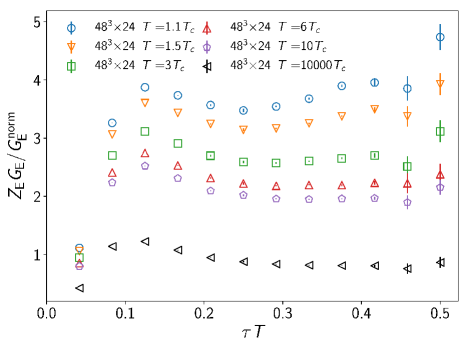
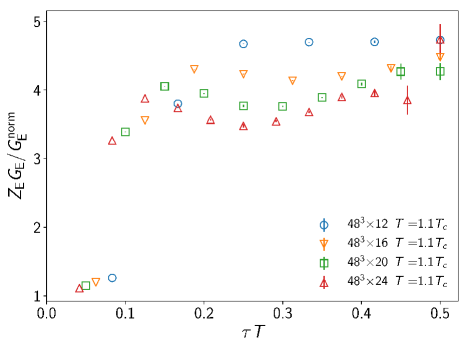
Figure 1: The chromoelectric field correlator from Eq. (1) normalized with Eq. (4). Top: all measured temperatures for $N_{\rm t}=24$. Bottom: all measured temporal extents $N_{\rm t}$ for the smallest temperature.

In order to reduce discretization errors we turn to a tree-level improvement procedure Sommer (1994); Meyer (2009), where the leading order results in the continuum (4) and the lattice perturbation theory are matched. The LO lattice perturbation theory gives Francis et al. (2011):

$$\frac{G_{\mathrm{E}}^{\mathrm{LO,lat}}(\tau)}{g^{2}C_{\rm F}} =\int_{-\pi}^{\pi}\frac{\mathop{\mathrm{d}^{3}q}}{(2\pi)^{3}}\frac{\tilde{q}^{2}e^{\bar{q}N_{\rm t}(1-\tau T)}+\tilde{q}^{2}e^{\bar{q}N_{\rm t}\tau T}}{3a^{4}\left(e^{\bar{q}N_{\rm t}}-1\right)\sinh(\bar{q})}\,,$$ (5)

where

$$\bar{q} =2\mathrm{arsinh}(\tilde{q}/2)\,,$$ (6)

$$\tilde{q}^{2} =\sum_{i=1}^{3}4\sin^{2}(q_{i}/2)\,.$$ (7)

The improved distance $\overline{\tau}$ is then defined so that $G_{\mathrm{E}}^{\mathrm{LO}}(\overline{\tau})=G_{\mathrm{E}}^{\mathrm{LO,lat}}(\tau)$. In Fig. 2, we show our results for $Z_{\mathrm{E}}G_{\mathrm{E}}^{\mathrm{imp}}(\tau)/G_{\mathrm{E}}^{\mathrm{norm}}=Z_{\mathrm{E}}G_{\mathrm{E}}(\overline{\tau})/G_{\mathrm{E}}^{\mathrm{norm}}$. From the figure, we can observe that after the tree-level improvement, the ratio $Z_{\mathrm{E}}G_{\mathrm{E}}/G_{\mathrm{E}}^{\mathrm{norm}}$ appears monotonically increasing with increasing $\tau T$ and has a decreasing slope as a function of temperature. At the highest temperature, $T=10^{4}\,T_{\rm c}$, we see a nearly horizontal $\tau$-independent line. Moreover, we observe a large reduction of cutoff effects for all temperatures when tree-level improvement is used. As an example, we show this reduction at the bottom of Fig. 2 for the lowest temperature, $T=1.1\,T_{\rm c}$. A similar reduction in the $N_{\rm t}$ dependence is seen at other temperatures. Due to its impact, we will use the tree level improvement for the rest of this paper, and therefore, unless otherwise indicated, drop the overline from $\overline{\tau}$ and the superscript "imp" from $G_{\mathrm{E}}^{\mathrm{imp}}$.

Figure 2: The chromoelectric field correlator from Eq. (1) normalized with Eq. (4) and tree-level improved with (5). Top: all measured temperatures for the biggest $N_{\rm t}=24$. Bottom: all measured temporal extents $N_{\rm t}$ for the smallest temperature.

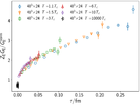
Figure 3: The data of Fig 2 in physical units.

The normalized chromoelectric correlator shown in Fig. 2 has a significant $\tau$-dependence. We conclude that the LO perturbative result does not capture the key features of the chromoelectric correlator. Only at the highest temperature, $T=10^{4}\,T_{\rm c}$, is the $\tau$-dependence of the correlator well described by the leading order result. One may wonder whether the observed behavior of the normalized chromoelectric correlator is due to thermal effects that are not present at leading order, like the physics of the heavy quark transport, or are due to higher-order effects at zero temperature. In order to answer this question, we show our lattice results in Fig. 3 as a function of $\tau$ in physical units rather than a function of $\tau T$. This figure shows that the ratio of the chromoelectric correlator to the free theory result is largely temperature independent implying that the chromoelectric correlator is dominated by the vacuum part of the spectral function. It thus becomes even more important to quantify the temperature dependence of the chromoelectric correlator. This can be done by considering the following ratio of the normalized correlator at a fixed value of $\beta$, but at two temperatures corresponding to temporal extents $N_{\rm t}$ and $2N_{\rm t}$. Lattice artifacts are canceled out in the double ratio:

$$R_{2}(N_{\rm t})=\frac{G_{\mathrm{E}}(N_{\rm t},\beta)}{G_{\mathrm{E}}^{\mathrm{norm}}(N_{\rm t})}\bigg{/}\frac{G_{\mathrm{E}}(2N_{\rm t},\beta)}{G_{\mathrm{E}}^{\mathrm{norm}}(2N_{\rm t})}\,.$$ (8)

Furthermore, if the LO result is a good approximation of the correlator and $\kappa/T^{3}$ is temperature independent, $R_{2}(N_{\rm t})$ should be 1 and independent of the temperature, while the temperature dependence of $\kappa/T^{3}$ will make this ratio different from 1 and also temperature dependent. The amount by which $R_{2}(N_{\rm t})$ deviates from 1 also depends on the value of $\kappa/T^{3}$: small values of $\kappa/T^{3}$ will result only in small deviations of $R_{2}(N_{\rm t})$ from 1. Our results for $R_{2}(N_{\rm t})$ are shown in Fig. 4. At the highest temperature the double ratio is consistent with 1 within errors, perhaps not surprisingly as at high temperatures the temperature dependence of $\kappa/T^{3}$ is expected to be logarithmic, and thus rather mild. At lower temperatures, however, we see deviations from 1 in the double ratio at the few-percent level, which increase with decreasing temperature and increasing $\tau T$. On the other hand, for $\tau T<0.2$ the double ratio is close to 1, implying that there the correlator is dominated by the $T=0$ part of the spectral function. In any case, thermal effects in the chromoelectric correlator, which encode the value of $\kappa$, are small, at the level of few percent. This fact implies that extracting $\kappa$ from lattice determinations of the chromoelectric correlator is challenging.

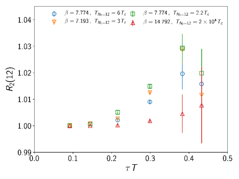
Figure 4: The ratio Eq. (8) of simulations with the same $\beta$ at different temperatures with $N_{\rm t}=12$.

Before extracting the heavy quark diffusion coefficient we need to address finite-volume effects and perform the continuum extrapolation of $Z_{\mathrm{E}}G_{\mathrm{E}}$. Most of our calculations have been performed using $N_{\rm s}=48$. To check for finite-volume effects for $N_{\rm t}=12$, we have performed calculations using spatial sizes $N^{3}_{\mathrm{s}}=24^{3},32^{3},48^{3}$ at two temperatures, $T=1.5\,T_{\rm c}$ and $T=10\,T_{\rm c}$. The smallest spatial volume here corresponds to the aspect ratio $N_{\rm s}/N_{\rm t}=2$. The detailed study of finite-volume effects is discussed in Appendix A. We find that the finite-volume effects are small, considerably smaller than other sources of error down to the aspect ratio $N_{\rm s}/N_{\rm t}=2$. Therefore, at the current level of precision, using a $N_{\rm s}=48$ lattice is sufficient even for $N_{\rm t}=24$.

Next, we perform the continuum extrapolations of $Z_{\mathrm{E}}G_{\mathrm{E}}$. The systematic errors in the renormalization constant estimated above are combined with the statistical errors of the chromoelectric correlator before performing the continuum extrapolation. In the interval $0.1\leq\tau T\leq 0.45$ we have a sufficient number of data points to perform the continuum extrapolations. We first interpolate the data for each $N_{\rm t}$ in $\tau T$ using ninth-order polynomials to estimate $Z_{\mathrm{E}}G_{\mathrm{E}}$ at common $\tau T$ values. We perform linear extrapolations in $1/N_{\rm t}^{2}=(aT)^{2}$ of $Z_{\mathrm{E}}G_{\mathrm{E}}$ at these $\tau T$ values using lattices with $N_{\rm t}=16,~{}20$, and $24$. As an example, we show the continuum extrapolation for selected values of $\tau T$ in Fig. 5. One can see that the $N_{\rm t}=12$ data do not lie in the $1/N_{\rm t}^{2}$ scaling region. Therefore, we also perform extrapolations to $N_{\rm t}=12$ data with a $(aT)^{4}$ term included. The difference between these continuum extrapolations is used as an estimate of the systematic error of the continuum result. The slope of the $a^{2}$ dependence is increasing with decreasing $\tau T$, as can be seen from Fig. 5. This is expected; the cutoff effects are larger at smaller $\tau T$. However, at the smallest value, $\tau T=0.1$, the slope of the $a^{2}$ dependence becomes smaller again contrary to expectations. We take this as an indication that the cutoff effects in this region cannot be described by a simple $a^{2}$ or $a^{2}+a^{4}$. As shown in Appendix A the slope of the $a^{2}$ dependence increases monotonically only till $\tau T\geq 0.175$. Therefore, we consider the continuum extrapolation to be reliable only for $\tau T\geq 0.175$. For an additional cross-check, we also perform the continuum extrapolation of the lattice data without tree-level improvement. This is discussed in Appendix A, where further details of the continuum extrapolations can be found.

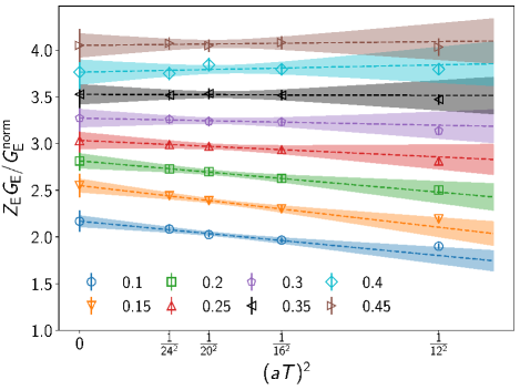
Figure 5: The continuum extrapolation. The lines represent the fit performed with the three largest $N_{\rm t}$’s at temperature $T=1.1\,T_{\rm c}$ at different values of $\tau T$, shown with different colors. The fitted line is extrapolated to 0 and to $1/12^{2}$ to show the quality of the fit compared to points at those locations. The point at zero includes the systematic error coming from the inclusion of the smallest lattice.

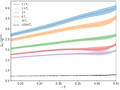
Figure 6: The continuum extrapolation for all temperatures as a function of $\tau T$.

The continuum-extrapolated chromoelectric correlator normalized by $G_{\mathrm{E}}^{\mathrm{norm}}$ is shown in Fig. 6 for all temperatures as function of $\tau T$. The continuum-extrapolated results share the general features of the tree-level-improved results at nonzero lattice spacing in terms of $\tau$ and temperature dependence. In particular, we see a strong dependence on $\tau T$, except for the highest temperature, indicating that the leading-order result does not capture the $\tau T$ dependence of $G_{\mathrm{E}}$. We will try to understand these features of the correlator in the next sections.

III Spectral functions and diffusion coefficient in perturbation theory

In order to determine the heavy quark diffusion coefficient $\kappa$ from the chromoelectric correlator $G_{\mathrm{E}}$, one has to use the relation between this correlator and the spectral function $\rho(\omega,T)$:

$$G_{\mathrm{E}}(\tau) =\int_{0}^{\infty}\frac{\mathop{\mathrm{d}\omega}}{\pi}\rho(\omega,T)K(\omega,\tau T)\,,$$ (9)

where

$$K(\omega,\tau T) =\frac{\cosh\left(\frac{\omega}{T}\left(\tau T-\frac{1}{2}\right)\right)}{\sinh\left(\frac{\omega}{2T}\right)}.$$

The heavy quark diffusion coefficient is determined in terms of $\rho$ through the Kubo formula Kapusta and Gale (2011)

$$\kappa\equiv\lim_{\omega\rightarrow 0}\frac{2T\rho(\omega,T)}{\omega}.$$ (10)

At the leading order of the perturbation theory, the spectral function is given by Caron-Huot et al. (2009):

$$\rho^{\mathrm{LO}}(\omega,T)=\frac{g^{2}(\mu_{\omega})C_{\rm F}\omega^{3}}{6\pi}\,,$$ (11)

where the coupling has been evaluated at the scale $\mu_{\omega}$. We use the five-loop running coupling constant in this work Tanabashi et al. (2018). At LO the scale $\mu_{\omega}$ is arbitrary. A natural choice is $\mu_{\omega}^{\mathrm{simple}}=\mathrm{max}(\omega,\pi T)$ Francis et al. (2015). The LO spectral function (11) gives $\kappa=0$.

At NLO, the perturbative calculation of $\rho(\omega,T)$ needs Hard-Thermal-Loop (HTL) resummation for $\omega\mathrel{\raise 1.29167pt\hbox{$<$\kern-7.5pt\lower 4.30554pt\hbox{$\sim$}}}m_{\mathrm{E}}$, with $m_{\mathrm{E}}$ being the LO Debye mass: $m_{\mathrm{E}}=\sqrt{N_{\rm c}/3}gT$ in the pure gauge theory. The full NLO result of $\rho(\omega,T)$ has been calculated in Ref. Burnier et al. (2010). The NLO spectral function provides the LO nonvanishing result for $\kappa$:

$$\frac{\kappa^{\mathrm{LO}}}{T^{3}}=\frac{g^{4}C_{\rm F}N_{\rm c}}{18\pi}\left[\ln\frac{2T}{m_{\mathrm{E}}}+\xi\right]\,,$$ (12)

where $\xi=\frac{1}{2}-\gamma_{\mathrm{E}}+\frac{\zeta^{\prime}(2)}{\zeta(2)}\simeq-0.64718$. For $\omega\mathrel{\raise 1.29167pt\hbox{$>$\kern-7.5pt\lower 4.30554pt\hbox{$\sim$}}}T$, there is no need for resummation when calculating the spectral function at NLO; the naive (nonresummed) NLO result for $\rho(\omega,T)$ in the pure gauge case reads

$$\rho_{\mathrm{naive}}(\omega,T)=$$ (13)

$$\frac{g^{2}C_{\rm F}\omega^{3}}{6\pi}\biggl{\{}1+\frac{g^{2}}{(4\pi)^{2}}\biggl{[}N_{\rm c}\biggl{(}\frac{11}{3}\ln\frac{\mu^{2}_{\omega}}{4\omega^{2}}+\frac{149}{9}-\frac{8\pi^{2}}{3}\biggr{)}\biggr{]}\biggr{\}}$$

$$+\frac{g^{2}C_{\rm F}}{6\pi}\frac{g^{2}}{2\pi^{2}}\biggl{\{}N_{\rm c}\int_{0}^{\infty}\!\mathop{\mathrm{d}q}\,n_{\mathrm{B{}}}(q)\biggl{[}(q^{2}+2\omega^{2})\ln\left|\frac{q+\omega}{q-\omega}\right|$$

$$+q\omega\biggl{(}\ln\frac{|q^{2}-\omega^{2}|}{\omega^{2}}-1\biggr{)}$$

$$+\frac{\omega^{4}}{q}\mathbbm{P}\biggl{(}\frac{1}{q+\omega}\ln\frac{q+\omega}{\omega}+\frac{1}{q-\omega}\ln\frac{\omega}{|q-\omega|}\biggr{)}\biggr{]}\biggr{\}}\,,$$

where $n_{\mathrm{B{}}}(q)=(\exp(q/T)-1)^{-1}$ is the Bose–Einstein distribution, $\mathbbm{P}$ takes the principal value, and $g^{2}\equiv g^{2}(\mu_{\omega})$. The first line of Eq. (13) gives the NLO $T=0$ contribution, and the subsequent lines carry the thermal effects. For the NLO $\rho(\omega,T)$, $\mu_{\omega}$ may be set such that the NLO $T=0$ contribution vanishes Burnier et al. (2010):

$$\ln(\mu_{\omega})=\ln(2\omega)+\frac{(24\pi^{2}-149)}{66}\,,$$ (14)

and the $T=0$ part of Eq. (13) reduces to Eq. (11). This is a convenient choice of scale for $\omega\gg T$. For $\omega\sim T$ or smaller a convenient choice of scale was proposed in Ref. Kajantie et al. (1997)

$$\ln(\mu_{\omega})=\ln(4\pi T)-\gamma_{\mathrm{E}}-\frac{1}{22}\,,$$ (15)

in the pure gauge case. We switch between these two scales when they become equal at $\omega\simeq 0.8903\,T$ Burnier et al. (2010).

The heavy quark diffusion coefficient has been calculated at NLO, and the result reads Caron-Huot and Moore (2008):

$$\frac{\kappa^{\mathrm{NLO}}}{T^{3}}=\frac{g^{4}C_{\rm F}N_{\rm c}}{18\pi}\left[\ln\frac{2T}{m_{\mathrm{E}}}+\xi+2.3302\frac{m_{\mathrm{E}}}{T}\right].$$ (16)

The NLO result for $\kappa$ cannot be replicated from currently known spectral functions as that would require $\rho(\omega,T)$ to be available at NNLO, which it is not. Both the LO and NLO results for $\kappa$ are obtained under the weak coupling assumption $m_{\mathrm{E}}~\ll T$. This condition, however, is not satisfied for most of the temperatures of interest. As a consequence, one obtains an unphysical behavior at LO i.e., that $\kappa$ becomes negative for $T<10^{3}\,T_{\rm c}$.

One can also calculate $\kappa$ using the kinetic theory. The corresponding expression reads Caron-Huot and Moore (2008, 2008):

$$\kappa^{\mathrm{LO}}= \frac{g^{4}C_{\rm F}}{12\pi^{3}}\int_{0}^{\infty}q^{2}\mathop{\mathrm{d}q}\int_{0}^{2q}\frac{p^{3}\mathop{\mathrm{d}p}}{(p^{2}+\Pi_{00})^{2}}$$ (17)

$$\times N_{\rm c}n_{\mathrm{B{}}}(q)(1+n_{\mathrm{B{}}}(q))\left(2-\frac{p^{2}}{q^{2}}+\frac{p^{4}}{4q^{4}}\right)\,.$$

If we do not expand in the temporal gluon self-energy, $\Pi_{00}(p)$, which is formally of order $g^{2}$, the above expression contains higher-order contributions to $\kappa$ as well. Therefore, the above expression can be considered as the resummed leading-order result. The temporal gluon self-energy depends on the gauge choice. For small momenta, it can be expanded as

$$\Pi_{00}(p)=m_{\mathrm{E}}^{2}-\frac{N_{\rm c}}{4}g^{2}Tp+...\,.$$ (18)

The first two terms in this expansion are gauge independent. We can take either the first term or the first and second terms in the above expression and evaluate the integral in Eq. (17) numerically. Only keeping the first term in the above expression for $\Pi_{00}$ already leads to a positive result, while keeping the second term as well leads to an enhancement of the $\kappa$ value. We present all the different perturbative results for $\kappa$ as a function of temperature in Fig. 7. The scale of the coupling is the one defined in Eq. (15).

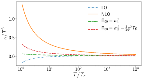
Figure 7: Perturbative estimates of $\kappa$ for the pure gauge theory as a function of temperature calculated at LO and NLO, as well as using the resummed leading-order expression (17).

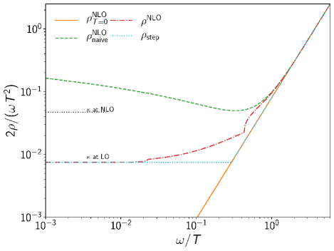
Figure 8: The perturbative spectral functions $\rho(\omega,T)$ at $T=10^{4}\,T_{\rm c}$ for different orders of perturbation theory. The dotted lines on the left indicate the perturbative estimates of $\kappa$ given by Eqs. (12) (LO) and (16) (NLO).

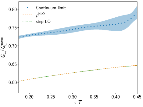
Figure 9: The chromoelectric correlator at $T=10^{4}\,T_{\rm c}$ calculated from the NLO spectral function (orange band) and the perturbative step form of the spectral function (green band). The orange band completely overlaps with the green band, and it is hardly distinguishable from it. The errors for both orange and green bands come from varying the scale by a factor of 2. In blue, we show the continuum limit of the $T=10^{4}\,T_{\rm c}$ lattice data.

At the highest temperature considered in this, $T=10^{4}\,T_{\rm c}$, study we expect that the NLO result can provide some guidance on the properties of the spectral function and on the $\tau$ dependence of the chromoelectric correlator. Therefore, in Fig. 8 we show different versions of the NLO spectral function, including the zero-temperature one. The full NLO spectral function can be described well by the simple $\kappa^{\mathrm{LO}}\omega/(2T)$ form for $\omega<0.02\,T$, while it approximately agrees with the $T=0$ result for $\omega>2\,T$. The full NLO result and the naive (unresummed) NLO result agree for $\omega>0.6\,T$. At small $\omega$, the naive NLO result is logarithmically divergent. This divergence cancels against contributions coming from the scale $m_{\mathrm{E}}$ in the resummed expression. We can model the spectral function by smoothly matching the $\kappa^{\mathrm{LO}}\omega/(2T)$ behavior at small $\omega$ with the zero-temperature spectral function at large $\omega$. We call this the perturbative step form. It is also shown in Fig. 8 by the blue dotted line. By using the NLO spectral function evaluated for $\mu=\mu_{\omega}$, we can calculate the corresponding chromoelectric correlator, which is shown in Fig. 9. Varying the renormalizarion scale by a factor of 2 around $\mu_{\omega}$ leads only to very small changes of the correlator, roughly corresponding to the width of the line in Fig. 9. We also calculate the chromoelectric correlator corresponding to the perturbative step form. The resulting correlator is indistinguishable from the one obtained using the NLO spectral function. This means that the additional structures in the spectral function in the region $0.02<\omega/T<0.6$ play no significant role when it comes to the correlator. We have also considered a perturbative step model using $\kappa^{\mathrm{NLO}}$. While using the NLO result for $\kappa$ significantly enhances the spectral function in the low $\omega$ region it only leads to a $0.2\%$ enhancement of the chromoelectric correlator compared to the one obtained using $\kappa^{\mathrm{LO}}$. Thus, the correlator is not sensitive to the small $\omega$ part of the spectral function at the highest temperature. At lower temperatures, $\kappa/T^{3}$ gets larger, and the contribution of the low $\omega$ part of the spectral functions is more prominent. Therefore, it is at lower temperatures that the value of $\kappa$ can be constrained by accurate calculations of the chromoelectric correlator.

While at $T=10^{4}\,T_{\rm c}$, one may expect the resummed NLO result to provide an adequate description of the spectral function, this is not expected at lower temperatures, because, as pointed out above, numerically $m_{\mathrm{E}}>T$. In particular, for $T<10^{3}\,T_{\rm c}$ the resummed spectral function turns negative at some point in the region $\omega<T$, thus implying that the resummed perturbative result is not applicable in this $\omega$ range. In Sec. V we will discuss the implications of this finding.

In Fig. 9, we also show the continuum limit of the chromoelectric correlator at the high temperature $T=10^{4}\,T_{\rm c}$ for comparison. The continuum-extrapolated lattice result of the chromoelectric correlator has the same shape as the NLO calculation. We note, however, that our continuum data differ from the perturbative curve by a factor 1.2, which indicates that the renormalization constant is not accurate. If we normalize the above lattice result to the correlator obtained from the NLO spectral function discussed above at $\tau T=0.19$, we find that the two agree within errors.

IV Short-time behavior of the lattice results on the electric correlator

The continuum results of $G_{\mathrm{E}}$ normalized by $G_{\mathrm{E}}^{\mathrm{norm}}$ show significant dependence on $\tau$. The analysis in Sec. II implies that this cannot be caused by thermal effects (cf. Figs. 3 and 4 ). The LO result does not take into account the effect of the running of the gauge coupling, and this could be the reason why $G_{\mathrm{E}}^{\mathrm{LO}}$, or equivalently $G_{\mathrm{E}}^{\mathrm{norm}}$ (which is the same up to a multiplicative factor) does not capture the $\tau$ dependence of the chromoelectric correlator. Therefore, as an alternative normalization we consider a correlator obtained from Eq. (9) using the zero-temperature NLO result for the spectral function with a running coupling constant evaluated at scale $\mu_{\omega}$ given by Eqs. (14) and (15). We label the corresponding correlator as $G_{\mathrm{E}}^{\mathrm{NLO+}}$.

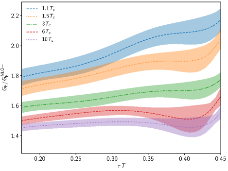
Figure 10: Continuum extrapolation for all temperatures as a function of $\tau T$.

	1.1	1.5	3	6	10	$10^{4}$
0.5$\mu_{\omega}$	1.82(5)	1.74(5)	1.61(3)	1.52(3)	1.47(2)	1.20(1)
1$\mu_{\omega}$	1.81(5)	1.73(5)	1.60(3)	1.51(3)	1.46(2)	1.20(1)
2$\mu_{\omega}$	1.84(5)	1.76(5)	1.62(3)	1.53(3)	1.48(2)	1.20(1)

Table 2: Normalization factor $C_{\mathrm{N}}$ for three different renormalization scales (rows) and for each measured temperature (columns) at $\tau T=0.19$.

The numerical results for $G_{\mathrm{E}}/G_{\mathrm{E}}^{\mathrm{NLO+}}$ are shown in Fig. 10. We see that this ratio increases less with increasing $\tau$. We expect that for small enough $\tau T$, one would see a plateau in $G_{\mathrm{E}}/G_{\mathrm{E}}^{\mathrm{NLO+}}$. This is not the case, however, because the continuum extrapolation is not reliable for $\tau T<0.17$, and for larger $\tau T$ there are some small thermal effects. On the other hand, given the uncertainties, we could still fit $G_{\mathrm{E}}/G_{\mathrm{E}}^{\mathrm{NLO+}}$ with a constant for $0.17\leq\tau T\leq 0.19$. This indicates that $G_{\mathrm{E}}^{\mathrm{NLO+}}$ captures the $\tau$ dependence of the chromoelectric correlator obtained on the lattice much better. However, even at the smallest $\tau$ the ratio $G_{\mathrm{E}}/G_{\mathrm{E}}^{\mathrm{NLO+}}$ is different from 1. This is most likely due to the fact that the one-loop result is not accurate for $Z_{\mathrm{E}}$. As shown in the previous section, even for the highest temperature, $T=10^{4}\,T_{\rm c}$, the NLO result is lower by a factor of 1.2, as seen in Fig. 9, although its $\tau$-dependence agrees well with the continuum extrapolated lattice data. Therefore, we introduce an additional normalization factor, $C_{\mathrm{N}}$ by normalizing the ratio $G_{\mathrm{E}}/G_{\mathrm{E}}^{\mathrm{NLO+}}$ to 1 at $\tau T=0.19$. To check the uncertainty of $C_{\mathrm{N}}$ due to the choice of the normalization point, we also consider $\tau T=0.175$ as a possible normalization point. Furthermore, we vary the scale $\mu_{\omega}$ by a factor of 2 around the optimal value when evaluating $C_{\mathrm{N}}$. The numerical values of $C_{\mathrm{N}}$ are shown in Tab. 2 for different temperatures. The dependence on the normalization point is shown in the systematic error and is of the same order as the scale dependence. The additional normalization constant $C_{\mathrm{N}}$ decreases with increasing temperature. This is due to the fact that the $\beta$ range used in the evaluation of the lattice correlator is increasing with increasing temperature, and the one-loop result is more reliable at large $\beta$ values. We will normalize $G_{\mathrm{E}}/G_{\mathrm{E}}^{\mathrm{NLO+}}$ with $C_{\mathrm{N}}$ given in Table 2 before comparing with the model spectral functions used for the extraction of $\kappa$.

V Modeling the spectral function and determination of $\kappa$

To obtain the heavy quark diffusion coefficient from the continuum-extrapolated lattice results, we need to assume some model for the spectral function. We will use the NLO results on the spectral function as well as $\kappa$ to guide us in this process. We also need to consider how sensitive the Euclidean-time chromoelectric correlator is to the spectral function in different $\omega$ regions. From the previous sections it is clear that $G_{E}$ is dominated by the large $\omega$ part of the spectral function and thermal effects in the spectral function contribute at the level of a few percent to the correlator.

It is reasonable to assume that at large enough $\omega$, perturbation theory is reliable even if the condition $m_{E}\ll T$ is not satisfied. This is because for large $\omega$ HTL resummation is not important, as will be detailed later. Certainly at zero temperature the perturbative calculation of $\rho(\omega,T)$ is reliable for $\omega\gg\Lambda_{\mathrm{QCD}}$. Therefore, we assume that for $\omega>\omega^{\mathrm{UV}}$ the spectral function is given by $\rho^{\mathrm{UV}}(\omega,T)$, which is calculated perturbatively. On the other hand, for sufficiently small $\omega$, the spectral function is given by

$$\rho^{\mathrm{IR}}(\omega,T)=\frac{\omega\kappa}{2T},$$ (19)

and we can assume that $\rho(\omega,T)=\rho^{\mathrm{IR}}(\omega,T)$ for $\omega<\omega^{\mathrm{IR}}$. In the region $\omega^{\mathrm{IR}}<\omega<\omega^{\mathrm{UV}}$, the form of the spectral function is not known, in general, and this lack of knowledge will generate an uncertainty in the determination of $\kappa$. Based on these considerations, we adopt the following procedure to estimate $\kappa$:

• For a given value of $\kappa$, we construct the model spectral function that is given by the NLO result at high energy, $\omega>\omega^{\mathrm{UV}}$, and by Eq. (19) at low energy, $\omega<\omega^{\mathrm{IR}}$.

• For intermediate $\omega$, namely $\omega^{\mathrm{IR}}\leq\omega\leq\omega^{\mathrm{UV}}$, we consider various forms of the spectral function such that the total spectral function is smooth, as described below.

• We match the continuum-extrapolated lattice result for the chromoelectric correlator to the correlator obtained from the model spectral function at small $\tau T$ and adjust the value of $\kappa$ to obtain the best description of the lattice result. We take care that $\tau T$ is not too small, so that the procedure is not affected by lattice artifacts.

• We estimate the uncertainties due to modeling the spectral function for $\omega^{\mathrm{IR}}\leq\omega\leq\omega^{\mathrm{UV}}$, due to the normalization point in $\tau T$, and due to the choice of the renormalization scale in the NLO result.

We consider two possible forms of the spectral functions that are continuous and are based on simple interpolations between the small $\omega$ (IR) region and the large $\omega$ (UV) region:

$$\rho_{\mathrm{line}}(\omega,T)=\rho^{\mathrm{IR}}(\omega,T)\theta(\omega^{\mathrm{IR}}-\omega)+$$ (20)

$$\left[\frac{\rho^{\mathrm{IR}}(\omega,T)-\rho^{\mathrm{UV}}(\omega,T)}{\omega^{\mathrm{IR}}-\omega^{\mathrm{UV}}}\left(\omega-\omega^{\mathrm{IR}}\right)+\rho^{\mathrm{IR}}(\omega,T)\right]\times$$

$$\theta(\omega-\omega^{\mathrm{IR}})\theta(\omega^{\mathrm{UV}}-\omega)+\rho^{\mathrm{UV}}(\omega,T)\theta(\omega-\omega^{\mathrm{UV}})\,,$$

and

$$\rho_{\mathrm{step}}(\omega,T)=\rho^{\mathrm{IR}}(\omega,T)\,\theta(\Lambda-\omega)+\rho_{T=0}^{\mathrm{UV}}(\omega,T)\,\theta(\omega-\Lambda)\,.$$ (21)

The latter case corresponds to $\omega^{\mathrm{IR}}=\omega^{\mathrm{UV}}=\Lambda$ and the value of $\Lambda$ is self-consistently determined by the continuity of the spectral function for a given $\kappa$. Thus, this model depends only on $\kappa$. In the former case additional considerations are needed to fix $\omega^{\mathrm{IR}}$ and $\omega^{\mathrm{UV}}$, which are described below. We will refer to these two forms as the line model and the step model, respectively.

The NLO result for the spectral function naturally interpolates between the IR and UV regions, but it is not reliable for small $\omega$ even at the highest temperature as discussed in Sec. III. However, it can provide some guidance on how to choose $\omega^{\mathrm{IR}}$ and $\omega^{\mathrm{UV}}$. As mentioned above, for $\omega>T$, HTL resummation may not be important, and the naive and resummed NLO result for the spectral function should agree. As discussed in Appendix B, the resummed and naive NLO results for the spectral function agree well for $\omega>2.2\,T$. Furthermore, the thermal contribution to $\rho(\omega,T)$ is about the same for $\omega>2.2\,T$ at the lowest and the highest temperature when normalized by $\omega T^{2}$. This indicates that the perturbative calculations are reliable for these values of $\omega$. Therefore, we choose $\omega^{\mathrm{UV}}=2.2\,T$. At the highest temperatures, the resummed NLO result is well described by the linear form given by Eq. (19) with $\kappa=\kappa^{\mathrm{LO}}$ for $\omega<0.02\,T$. Therefore, $\omega^{\mathrm{IR}}=0.01\,T$ appears to be a reasonable choice. The NLO result for $\kappa$ is significantly larger than the LO result, implying that the spectral function at low $\omega$ is also larger and therefore will match $\rho^{\mathrm{UV}}(\omega,T)$ at larger $\omega$. We find that $\rho^{\mathrm{IR}}(\omega,T)$ and $\rho^{\mathrm{UV}}(\omega,T)$ are equal at around $\omega=0.4\,T$. Therefore, besides $\omega^{\mathrm{IR}}=0.01\,T$, we will also use $\omega^{\mathrm{IR}}=0.4\,T$ and $\omega^{\mathrm{IR}}=1\,T$ in our analysis.

In Fig. 11 we show the spectral functions obtained from Eqs. (20) and (21), assuming $\kappa=\kappa^{\mathrm{NLO}}$ in $\rho_{\mathrm{step}}$ and $\rho_{\mathrm{line}}$, and three different $\omega^{\mathrm{IR}}$ at three representative temperatures, $T=1.1\,T_{\rm c},~{}6\,T_{\rm c}$, and $10^{4}\,T_{\rm c}$. From the figure, we see that at the lowest temperature, the $\rho_{\mathrm{step}}(\omega,T)$ model matches the UV behavior at larger $\omega$ without the dip around $\omega\sim T$ of the $\rho_{\mathrm{line}}(\omega,T)$ model. The $\rho_{\mathrm{line}}$ form with $\omega^{\mathrm{IR}}=0.01\,T$ and $\rho_{\mathrm{step}}$ provide upper and lower bounds for the spectral function at $T=1.1\,T_{\rm c}$. The picture is the same for $T=1.5\,T_{\rm c}$ and $T=3\,T_{\rm c}$. At $T=6\,T_{\rm c}$, all forms of the spectral functions provide nearly identical results. At the highest two temperatures, the possible choices of the spectral functions are limited by $\rho_{\mathrm{line}}$ with $\omega^{\mathrm{IR}}=0.01\,T$ and $\omega^{\mathrm{IR}}=T$.

Using the models for the spectral functions described above, we have calculated the corresponding Euclidean-time chromoelectric correlators for different values of $\kappa$ and compared these with the continuum-extrapolated lattice results at each temperature to estimate the heavy quark diffusion coefficient. As discussed in the previous section, the continuum-extrapolated lattice results need an additional renormalization because the one-loop renormalization constant, $Z_{E}$, is not accurate. Therefore, we have matched the correlator obtained from the model spectral function to the continuum-extrapolated lattice data at $\tau T=0.19$. The resulting multiplicative constants $C_{N}$ are slightly different from those shown in Table 2. This is because the correlators obtained from the model spectral functions are slightly different from $G_{\mathrm{E}}^{\mathrm{NLO+}}$ at $\tau T=0.19$ due to the thermal contribution. We demonstrate this procedure in Appendix B for different model spectral functions. Different forms give different values of $\kappa$, and this is the dominant source of systematic error in the determination of $\kappa$. We have also studied the dependence of $\kappa$ on the choice of the normalization point in $\tau$ and the choice of the renormalization scale. Choosing the normalization point in the range $0.17\leq\tau T\leq 0.19$ leads to an 8% variation in the resulting $\kappa$. Varying the renormalization scale by a factor of 2 results in a similar variation.

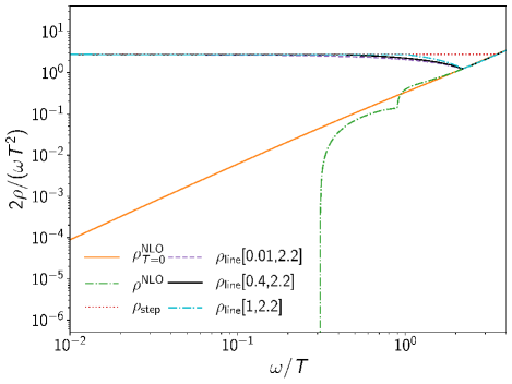
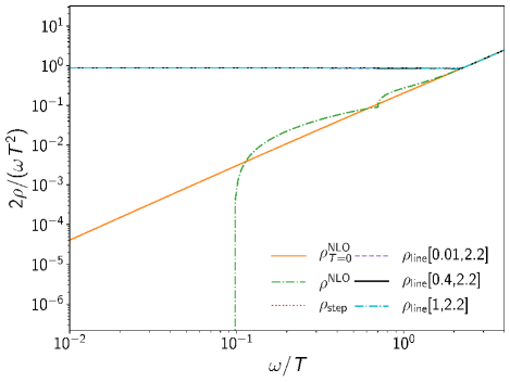
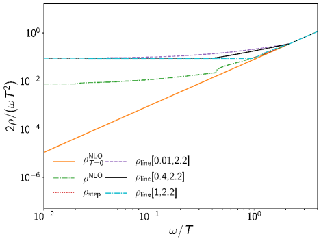
Figure 11: The shapes of different spectral function models $\rho(\omega,T)$ at (from top to bottom) $T=1.1\,T_{\rm c}$, $T=6\,T_{\rm c}$, and $T=10^{4}\,T_{\rm c}$. The arguments of $\rho_{\mathrm{line}}$ in square brackets stand for $[\omega^{\mathrm{IR}},\omega^{\mathrm{UV}}]$.

Putting everything together we obtain the following estimates for the heavy quark diffusion coefficient from the analysis:

$$1.91<\frac{\kappa}{T^{3}}<5.4\; \;T=1.1\,T_{\rm c}\,,$$ for (22)

$$1.31<\frac{\kappa}{T^{3}}<3.64\; \;T=1.5\,T_{\rm c}\,,$$ for (23)

$$0.63<\frac{\kappa}{T^{3}}<2.20\; \;T=3\,T_{\rm c}\,,$$ for (24)

$$0.43<\frac{\kappa}{T^{3}}<1.05\; \;T=6\,T_{\rm c}\,,$$ for (25)

$$0<\frac{\kappa}{T^{3}}<0.72\; \;T=10\,T_{\rm c}\,,$$ for (26)

$$0<\frac{\kappa}{T^{3}}<0.10\; \;T=10^{4}\,T_{\rm c}\,,$$ for (27)

although one should be reminded that, as discussed at the end of Sec. III, the lattice data are weakly sensitive to $\kappa$ at the highest temperature. The dominant uncertainty in the above result comes from the form of the spectral function used in the analysis and the uncertainty of the continuum-extrapolated lattice results.

We compare our result on $\kappa$ with the results of other lattice studies Ding et al. (2012); Meyer (2011); Francis et al. (2011); Banerjee et al. (2012); Francis et al. (2015) in terms of the spatial diffusion coefficient $D_{s}$, which is given by the relation $\kappa/T^{3}=2/(D_{s}T)$, in the temperature range $T_{\rm c}-3\,T_{\rm c}$. This is shown in Fig. 12. We see that our results agree well with the other lattice determinations, with the exception of the one in Ref. Ding et al. (2012) that is based on charmonium correlators. This is likely due to the fact that the determination of $D_{s}$ from the quarkonium correlators is not accurate, since the width of the transport peak is difficult to determine Petreczky and Teaney (2006); Petreczky (2009).

The temperature dependence of the heavy quark diffusion coefficient in the entire temperature region is shown in Fig. 13. We clearly see the temperature dependence of $\kappa^{3}/T$. The $\kappa$ obtained on the lattice is not incompatible with the NLO result given the large errors. Inspired by this, we fit the temperature dependence of the lattice result by modeling it on Eq. (16) but keeping the coefficient of $m_{\mathrm{E}}/T$ as a free parameter $C$. From the fit, we obtain $C=3.81(1.33)$, which is larger than the NLO perturbative result $C\approx 2.3302$.

We note that our result is significantly larger than the simple holographic estimate Kovtun et al. (2003): $2\pi D_{s}T=1$. However, more recent holographic estimates Andreev (2018) are close to our results. Finally, comparing with more experimental quantities, we note that our result for $D_{s}$ at the lowest temperature is in agreement with the calculations of $D$ Tolos and Torres-Rincon (2013) and $\bar{\mathrm{B}}$ Torres-Rincon et al. (2014) mesons propagating in a medium of light hadrons, which find $2\pi D_{s}T\sim 5$ for $T\approx T_{\rm c}$, but much smaller than an earlier pion gas study Abreu et al. (2011) that found $2\pi D_{s}T\approx 17$ for $T\approx T_{\rm c}$. Experimental determinations of the D-meson azimuthal anisotropy coefficient $\nu_{2}$ at ALICE Acharya et al. (2018) and STAR Adamczyk et al. (2017) estimate at $T\approx T_{\rm c}$ that $\kappa/T^{3}\approx 1.8-8.38$ and $\kappa/T^{3}\approx 1.05-6.28$, respectively. These are in agreement with our findings. All these experimental determinations include mass-dependent contributions, while our determination of $\kappa$ is in the heavy quark limit. Therefore the two should agree up to $1/m$ corrections.

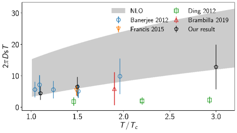
Figure 12: Our results compared to existing lattice studies. The shaded band shows the perturbative behavior (16) and the effect of the scale $\mu_{\omega}$ being varied by a factor of 2.

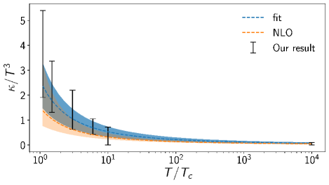
Figure 13: Temperature dependence of our results compared to the NLO result. The shaded bands include the errors coming from varying the scale by a factor of 2. The blue band also includes the statistical error.

VI Conclusions

In this paper, we have studied the chromoelectric correlator, $G_{\mathrm{E}}$ at finite temperature on the lattice with the aim of extracting the heavy quark diffusion coefficient $\kappa$. The calculations have been performed in quenched QCD (SU(3) gauge theory) in order to obtain small statistical errors with the help of the multilevel algorithm. We have studied the dependence of the chromoelectric correlator on the Euclidean time, $\tau$, in a wide temperature range in order to enable the comparison with weak coupling results. It turned out that the $\tau$-dependence of the electric correlator is poorly captured by the leading order result. Going beyond the leading-order result and incorporating the effect of the running coupling in the corresponding spectral function results in a correlation function $G_{\mathrm{E}}^{\mathrm{NLO+}}$ that can capture the $\tau$-dependence of the lattice result much better.

To fully describe the $\tau$-dependence of $G_{\mathrm{E}}$ calculated on the lattice, the effect of $\kappa$ encoded in the low $\omega$ part of the chromoelectric spectral function has to be considered. At high $\omega$, we have used forms of the spectral function that are motivated by the next-to-leading-order perturbative results. Fitting the lattice results on $G_{\mathrm{E}}$, we have obtained values of $\kappa$ at different temperatures. We observe that the sensitivity of the chromoelectric correlator to $\kappa$ is small, varying from a few percent at the lowest temperatures to sub-percent at the highest temperatures. This finding is corroborated by a model-independent analysis of the chromoelectric correlator, cf. Figs. 3 and 4. It is this small sensitivity that makes the lattice determination of $\kappa$ quite challenging. Our main result is summarized in Fig. 13, which shows the temperature dependence of the heavy quark diffusion coefficient. For $T<2\,T_{\rm c}$, our results agree with other lattice determinations, while at higher temperatures, they appear consistent with the NLO result.

One of the shortcomings of the present analysis is the use of the one-loop result for the renormalization constant, $Z_{\mathrm{E}}$, which, as we argued, is not reliable. The use of tadpole-improved one-loop perturbation theory will not help, since it will make $Z_{\mathrm{E}}$ even larger, while in order to achieve agreement of the lattice and NLO results at small $\tau$, we need a smaller $Z_{\mathrm{E}}$ than the one-loop result. Clearly, a nonperturbative renormalization procedure will be needed, but this is beyond the scope of the present paper.

Appendix A Infinite-volume limit and continuum extrapolation

To check to what extent using lattices with an aspect ratio $N_{\rm s}/N_{\rm t}$ smaller than 4 leads to visible finite-volume effects, we have performed calculations at two temperatures, $T=1.5\,T_{\rm c}$ and $T=10\,T_{\rm c}$, on $N_{\rm s}^{3}\times 12$ lattices with $N_{\rm s}=24,~{}32$, and $48$. The numerical results are shown in Fig. 14 for some representative values of $\tau T$. As one can see from the figure, the finite-volume effects are small. We have also attempted to perform an infinite-volume extrapolation by fitting the lattice results with a $1/N_{s}^{3}$ form. The corresponding fits are shown in the figure as lines and bands together with the infinite-volume result. It is clear from the figure that the differences between the infinite-volume result and the lattice results with different $N_{\rm s}$ values are of the order of the statistical errors. Therefore, the use of $N_{\rm s}=48$ is justified.

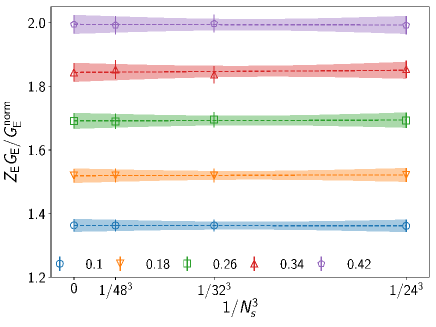
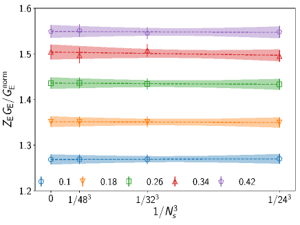
Figure 14: Finite-volume effects for several $\tau T$ values presented with different colors at $T=1.5\,T_{\rm c}$ (left) and $T=10\,T_{\rm c}$ (right). The lines and bands correspond to the $1/N_{\rm s}^{2}$ fits and their uncertainties.

As discussed in the main text, to obtain the continuum result for the chromoelectric correlator, we first perform the interpolation in $\tau T$, and then for each value of $\tau T$ we perform the continuum extrapolation using the $a/N_{\rm t}^{2}$ form without $N_{\rm t}=12$ data or using the $a/N_{\rm t}^{2}+b/N_{\rm t}^{4}$ form with $N_{\rm t}=12$ data included ($a$ and $b$ are fit constants). We have demonstrated this procedure in Fig. 5 for $T=1.1\,T_{c}$. In Fig. 15, we show this procedure for other temperatures: $T=1.5\,T_{\rm c}$, $3.0\,T_{\rm c}$, $6\,T_{\rm c}$, and $T=10^{4}\,T_{\rm c}$. We do not show the analysis for $10\,T_{\rm c}$, as it looks similar to the one for $T=10^{4}\,T_{\rm c}$. From the figure, we see that the slope of the $1/N_{\rm t}^{2}$ dependence increases with decreasing $\tau T$ as expected, since the cutoff dependence is larger for smaller $\tau T$. But for the smallest $\tau T$, we do not see this tendency. To understand the situation better, we show the coefficient of the $1/N_{\rm t}^{2}$ term in the continuum extrapolation as a function of $\tau T$ in Fig. 16. The coefficient of the $1/N_{\rm t}^{2}$ term decreases monotonically as $\tau T$ decreases. For this coefficient, the minimum of the absolute value is reached at $\tau T=0.32$ instead of at the largest available $\tau T$. Note, however, that this is somewhat accidental, as the coefficient changes sign around this value of $\tau T$. Also, the errors for $0.3<\tau<0.4$ are quite large. More importantly for us, the absolute value of the coefficient increases when we decrease $\tau T$ from 0.3 to 0.175, and then either flattens off or decreases if $\tau T$ is further decreased. We take this as an indication that the continuum limit is not reliable for $\tau T<0.175$.

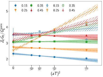
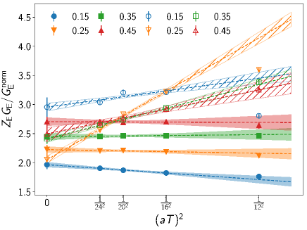
Figure 15: The continuum extrapolation of the chromoelectric correlator for $T=1.5\,T_{\rm c}$ and $T=3.0\,T_{\rm c}$ (top panels) and for $T=6.0\,T_{\rm c}$ and $T=10^{4}\,T_{\rm c}$ (bottom panels). The filled symbols and solid bands correspond to the extrapolation of the tree-level-improved lattice data, while the open symbols and patterned bands correspond to the extrapolations of the lattice data without tree-level improvement. The different colors correspond to different $\tau T$ values.

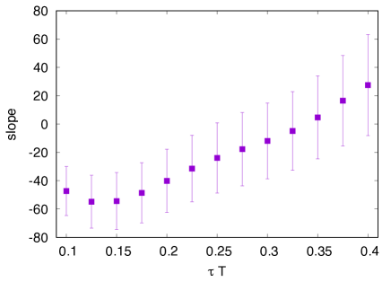
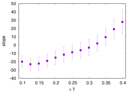
Figure 16: The coefficient of the $1/N_{\rm t}^{2}$ dependence as a function of $\tau$ for $T=1.5\,T_{\rm c}$ (left) and $T=10\,T_{\rm c}$ (right).

We also perform continuum extrapolations using lattice data without tree-level improvement and the corresponding results are also shown in Fig. 15 as open symbols. In this case, the continuum limit is always approached from above. The continuum-extrapolated result from tree-level-improved lattice data and the unimproved lattice data agree within errors for $\tau T\geq 0.25$. In the absence of tree-level improvement, the continuum extrapolations for smaller $\tau T$ are not reliable.

Appendix B Modeling of the spectral function and $\kappa$ determination

In order to understand the main features of the perturbative spectral function corresponding to the chromoelectric correlator at NLO, in Fig. 17 we show the quantity $2(\rho(\omega,T)-\rho(\omega)_{T=0}^{\mathrm{NLO}})/(\omega T^{2})$ calculated with and without HTL resummation at the lowest and highest temperatures. The plotted quantity gives $\kappa$ in the $\omega\rightarrow 0$ limit. The naive (unresummed) result is logarithmically divergent at small $\omega$. On the other hand, for $\omega>2.2\,T$, the resummed and the naive results agree well. This indicates that the NLO calculation is valid in this $\omega$ range. We also see that for $2.2<\omega/T<10$, the naive and resummed NLO expressions are negative, and their shapes are independent of the temperature.

In Fig. 17 we also show the two model spectral functions (line model and step model), where we use $\kappa=2.75\,T^{3}$ for the lowest temperature and $\kappa=0.088\,T^{3}$ for the highest one. At the lowest temperature, the step model has a larger finite-temperature part than the linear model, while at the highest temperature, the opposite is true. The two models also have somewhat different UV behavior. The step model is matched to the zero-temperature spectral function and thus ignores the thermal correction in the region $2.2<\omega/T<10$, while the line model incorporates this. The two models thus allow us to extract $\kappa$ using a set of reasonable assumptions about the large-$\omega$ behavior of the spectral function.

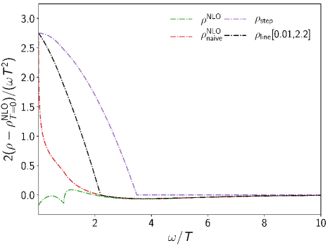
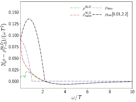
Figure 17: The NLO $T=0$ spectral function subtracted from different models or perturbative curves at $T=1.1\,T_{\rm c}$ (left) and $T=10^{4}\,T_{\rm c}$ (right). See the text for further specifications.

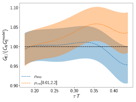
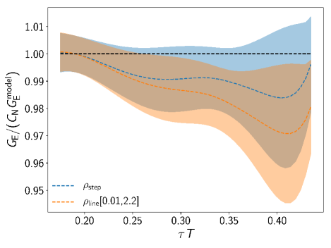
Figure 18: The ratio of the continuum-extrapolated chromoelectric correlator obtained on the lattice and the correlator obtained within the line model (orange band) and the step model (blue band) for $1.1\,T_{\rm c}$ and $\kappa=2.75\,T^{3}$ (left), and for $10^{4}\,T_{\rm c}$ and $\kappa=0.05\,T^{3}$ (right). The bands show the errors originating from lattice effects and from varying the scale by a factor of 2.

We match the chromoelectric correlator $G_{\mathrm{E}}^{\mathrm{model}}$, obtained from the above model spectral functions at $\tau T=0.19$ to the continuum-extrapolated lattice result to find the optimal value of $\kappa$. We demonstrate this procedure in Fig. 18 where we show the continuum lattice result for the lowest and the highest temperatures divided by the corresponding $G_{\mathrm{E}}^{\mathrm{model}}$. For a given spectral function and the appropriately chosen $\kappa$ this ratio should be close to 1. Since the errors of the continuum-extrapolated lattice result are sizable we get a range of $\kappa$ that is compatible with the lattice result. In Fig. 18 we show the results for $\kappa=2.75\,T^{3}$ and $\kappa=0.05\,T^{3}$, and for $T=1.1\,T_{\rm c}$ and $T=10^{4}\,T_{\rm c}$, respectively. These $\kappa$ values are chosen to be in the middle of the quoted ranges (see Eqs. (22) and (27)). At the lowest temperature for the given $\kappa$ the step form and the line form seem to be on the opposite side compared to the lattice result, while at the highest temperature the step form clearly gives a better description of the lattice data on average. We see that the optimal value of $\kappa$ strongly depends on the assumed form, especially at high temperatures.

References

- Busza et al. (2018) W. Busza, K. Rajagopal, and W. van der Schee, Ann. Rev. Nucl. Part. Sci., 68, 339 (2018), arXiv:1802.04801 [hep-ph] .
- Shuryak and Zahed (2004) E. V. Shuryak and I. Zahed, Phys. Rev., C70, 021901 (2004), arXiv:hep-ph/0307267 [hep-ph] .
- Shuryak (2004) E. Shuryak, Heavy ion reaction from nuclear to quark matter. Proceedings, International School of Nuclear Physics, 25th Course, Erice, Italy, September 16-24, 2003, Prog. Part. Nucl. Phys., 53, 273 (2004), arXiv:hep-ph/0312227 [hep-ph] .
- Beraudo et al. (2018) A. Beraudo et al., Nucl. Phys., A979, 21 (2018), arXiv:1803.03824 [nucl-th] .
- Moore and Teaney (2005) G. D. Moore and D. Teaney, Phys. Rev., C71, 064904 (2005), arXiv:hep-ph/0412346 [hep-ph] .
- Svetitsky (1988) B. Svetitsky, Phys. Rev., D37, 2484 (1988).
- Caron-Huot and Moore (2008) S. Caron-Huot and G. D. Moore, JHEP, 02, 081 (2008a), arXiv:0801.2173 [hep-ph] .
- Herzog et al. (2006) C. P. Herzog, A. Karch, P. Kovtun, C. Kozcaz, and L. G. Yaffe, JHEP, 07, 013 (2006), arXiv:hep-th/0605158 [hep-th] .
- Casalderrey-Solana and Teaney (2006) J. Casalderrey-Solana and D. Teaney, Phys. Rev., D74, 085012 (2006), arXiv:hep-ph/0605199 [hep-ph] .
- Aarts and Martinez Resco (2002) G. Aarts and J. M. Martinez Resco, JHEP, 04, 053 (2002), arXiv:hep-ph/0203177 [hep-ph] .
- Petreczky and Teaney (2006) P. Petreczky and D. Teaney, Phys. Rev., D73, 014508 (2006), arXiv:hep-ph/0507318 [hep-ph] .
- Petreczky (2009) P. Petreczky, Eur. Phys. J. C, 62, 85 (2009), arXiv:0810.0258 [hep-lat] .
- Ding et al. (2012) H. T. Ding, A. Francis, O. Kaczmarek, F. Karsch, H. Satz, and W. Soeldner, Phys. Rev., D86, 014509 (2012), arXiv:1204.4945 [hep-lat] .
- Ding et al. (2019) H.-T. Ding, O. Kaczmarek, A.-L. Kruse, R. Larsen, L. Mazur, S. Mukherjee, H. Ohno, H. Sandmeyer, and H.-T. Shu, Proceedings, 27th International Conference on Ultrarelativistic Nucleus-Nucleus Collisions (Quark Matter 2018): Venice, Italy, May 14-19, 2018, Nucl. Phys., A982, 715 (2019), arXiv:1807.06315 [hep-lat] .
- Lorenz et al. (2020) A.-L. Lorenz, H.-T. Ding, O. Kaczmarek, H. Ohno, H. Sandmeyer, and H.-T. Shu, PoS, LATTICE2019, 207 (2020), arXiv:2002.00681 [hep-lat] .
- Borsanyi et al. (2014) S. Borsanyi et al., JHEP, 04, 132 (2014), arXiv:1401.5940 [hep-lat] .
- Boguslavski et al. (2020) K. Boguslavski, A. Kurkela, T. Lappi, and J. Peuron, in 28th International Conference on Ultrarelativistic Nucleus-Nucleus Collisions (2020) arXiv:2001.11863 [hep-ph] .
- Boguslavski et al. (2020) K. Boguslavski, A. Kurkela, T. Lappi, and J. Peuron, JHEP, 09, 077 (2020b), arXiv:2005.02418 [hep-ph] .
- Brambilla et al. (2017) N. Brambilla, M. A. Escobedo, J. Soto, and A. Vairo, Phys. Rev., D96, 034021 (2017), arXiv:1612.07248 [hep-ph] .
- Brambilla et al. (2018) N. Brambilla, M. A. Escobedo, J. Soto, and A. Vairo, Phys. Rev., D97, 074009 (2018), arXiv:1711.04515 [hep-ph] .
- Brambilla et al. (2019) N. Brambilla, M. A. Escobedo, A. Vairo, and P. Vander Griend, Phys. Rev., D100, 054025 (2019), arXiv:1903.08063 [hep-ph] .
- Caron-Huot et al. (2009) S. Caron-Huot, M. Laine, and G. D. Moore, JHEP, 04, 053 (2009), arXiv:0901.1195 [hep-lat] .
- Meyer (2011) H. B. Meyer, New J. Phys., 13, 035008 (2011), arXiv:1012.0234 [hep-lat] .
- Francis et al. (2011) A. Francis, O. Kaczmarek, M. Laine, and J. Langelage, Proceedings, 29th International Symposium on Lattice field theory (Lattice 2011): Squaw Valley, Lake Tahoe, USA, July 10-16, 2011, PoS, LATTICE2011, 202 (2011), arXiv:1109.3941 [hep-lat] .
- Banerjee et al. (2012) D. Banerjee, S. Datta, R. Gavai, and P. Majumdar, Phys. Rev., D85, 014510 (2012), arXiv:1109.5738 [hep-lat] .
- Francis et al. (2015) A. Francis, O. Kaczmarek, M. Laine, T. Neuhaus, and H. Ohno, Phys. Rev., D92, 116003 (2015a), arXiv:1508.04543 [hep-lat] .
- Altenkort et al. (2019) L. Altenkort, O. Kaczmarek, L. Mazur, and H.-T. Shu, PoS, LATTICE2019, 204 (2019), arXiv:1912.11248 [hep-lat] .
- Lüscher and Weisz (2001) M. Lüscher and P. Weisz, JHEP, 09, 010 (2001), arXiv:hep-lat/0108014 [hep-lat] .
- Bazavov et al. (2018) A. Bazavov, P. Petreczky, and J. H. Weber, Phys. Rev., D97, 014510 (2018a), arXiv:1710.05024 [hep-lat] .
- Bazavov et al. (2013) A. Bazavov, H. T. Ding, P. Hegde, F. Karsch, C. Miao, S. Mukherjee, P. Petreczky, C. Schmidt, and A. Velytsky, Phys. Rev., D88, 094021 (2013), arXiv:1309.2317 [hep-lat] .
- Ding et al. (2015) H. T. Ding, S. Mukherjee, H. Ohno, P. Petreczky, and H. P. Schadler, Phys. Rev., D92, 074043 (2015), arXiv:1507.06637 [hep-lat] .
- Bazavov et al. (2016) A. Bazavov, N. Brambilla, H. T. Ding, P. Petreczky, H. P. Schadler, A. Vairo, and J. H. Weber, Phys. Rev., D93, 114502 (2016), arXiv:1603.06637 [hep-lat] .
- Bazavov et al. (2018) A. Bazavov, N. Brambilla, P. Petreczky, A. Vairo, and J. H. Weber (TUMQCD), Phys. Rev., D98, 054511 (2018b), arXiv:1804.10600 [hep-lat] .
- Bazavov et al. (2019) A. Bazavov et al., Phys. Rev. D, 100, 094510 (2019), arXiv:1908.09552 [hep-lat] .
- Burnier et al. (2010) Y. Burnier, M. Laine, J. Langelage, and L. Mether, JHEP, 08, 094 (2010), arXiv:1006.0867 [hep-ph] .
- Lüscher (2010) M. Lüscher, JHEP, 08, 071 (2010), [Erratum: JHEP 03, 092 (2014)], arXiv:1006.4518 [hep-lat] .
- Francis et al. (2015) A. Francis, O. Kaczmarek, M. Laine, T. Neuhaus, and H. Ohno, Phys. Rev., D91, 096002 (2015b), arXiv:1503.05652 [hep-lat] .
- Christensen and Laine (2016) C. Christensen and M. Laine, Phys. Lett., B755, 316 (2016), arXiv:1601.01573 [hep-lat] .
- Sommer (1994) R. Sommer, Nucl. Phys., B411, 839 (1994), arXiv:hep-lat/9310022 [hep-lat] .
- Meyer (2009) H. B. Meyer, JHEP, 06, 077 (2009), arXiv:0904.1806 [hep-lat] .
- Kapusta and Gale (2011) J. Kapusta and C. Gale, Finite-temperature field theory: Principles and applications, Cambridge Monographs on Mathematical Physics (Cambridge University Press, 2011) ISBN 978-0-521-17322-3, 978-0-521-82082-0, 978-0-511-22280-1.
- Tanabashi et al. (2018) M. Tanabashi et al. (Particle Data Group), Phys. Rev., D98, 030001 (2018).
- Kajantie et al. (1997) K. Kajantie, M. Laine, K. Rummukainen, and M. E. Shaposhnikov, Nucl. Phys., B503, 357 (1997), arXiv:hep-ph/9704416 [hep-ph] .
- Caron-Huot and Moore (2008) S. Caron-Huot and G. D. Moore, Phys. Rev. Lett., 100, 052301 (2008b), arXiv:0708.4232 [hep-ph] .
- Kovtun et al. (2003) P. Kovtun, D. T. Son, and A. O. Starinets, JHEP, 10, 064 (2003), arXiv:hep-th/0309213 [hep-th] .
- Andreev (2018) O. Andreev, Mod. Phys. Lett. A, 33, 1850041 (2018), arXiv:1707.05045 [hep-ph] .
- Tolos and Torres-Rincon (2013) L. Tolos and J. M. Torres-Rincon, Phys. Rev. D, 88, 074019 (2013), arXiv:1306.5426 [hep-ph] .
- Torres-Rincon et al. (2014) J. M. Torres-Rincon, L. Tolos, and O. Romanets, Phys. Rev. D, 89, 074042 (2014), arXiv:1403.1371 [hep-ph] .
- Abreu et al. (2011) L. M. Abreu, D. Cabrera, F. J. Llanes-Estrada, and J. M. Torres-Rincon, Annals Phys., 326, 2737 (2011), arXiv:1104.3815 [hep-ph] .
- Acharya et al. (2018) S. Acharya et al. (ALICE), Phys. Rev. Lett., 120, 102301 (2018), arXiv:1707.01005 [nucl-ex] .
- Adamczyk et al. (2017) L. Adamczyk et al. (STAR), Phys. Rev. Lett., 118, 212301 (2017), arXiv:1701.06060 [nucl-ex] .