Quadrilateral meshes for PSLGs

Abstract.

We prove that every planar straight line graph with $n$ vertices has a conforming quadrilateral mesh with $O(n^{2})$ elements, all angles $\leq 120^{\circ}$ and all new angles $\geq 60^{\circ}$. Both the complexity and the angle bounds are sharp.

1. Introduction

The purpose of this paper is to prove:

Theorem 1.1.

Suppose $\Gamma$ is a planar straight line graph with $n$ vertices. Then $\Gamma$ has a conforming quadrilateral mesh with $O(n^{2})$ elements, all angles $\leq 120^{\circ}$ and all new angles $\geq 60^{\circ}$.

The precise definitions of all the terminology will be given in the next few sections, but briefly, this means that each face of $\Gamma$ (each bounded complementary component) can be meshed with quadrilaterals so that the meshes are consistent across the edges of $\Gamma$ and all angles are in the interval $[60^{\circ},120^{\circ}]$ except when forced to be smaller by two edges of $\Gamma$ that meet at an angle $<60^{\circ}$.

Bern and Eppstein showed in [2] that any simple polygon $P$ has a linear sized quadrilateral mesh with all angles $\leq 120^{\circ}$. They also used Euler’s formula to prove that any quadrilateral mesh of a regular hexagon must contain an angle of measure $\geq 120^{\circ}$. Thus the upper angle bound is sharp. Moreover, if a polygon contains an angle of measure $120^{\circ}+\epsilon$, $\epsilon>0$, then this angle must be subdivided in the mesh (in order to achieve the upper bound), giving at least one new angle $\leq 60^{\circ}+\epsilon/2$. Thus the $60^{\circ}$ lower bound is also sharp. In [6] I showed that every simple polygon has a linear sized quadrilateral mesh with all angles $\leq 120^{\circ}$ and all new angles $\geq 60^{\circ}$. Theorem 1.1 extends this result to planar straight line graphs (PSLGs). The complexity bound increases from $O(n)$ to $O(n^{2})$, but this is necessary: see Figure 1.

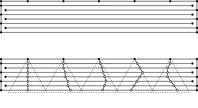
Figure 1. Consider a vertex $v$ along the top edge of the illustrated PSLG. Any mesh of this PSLG with all angles $\leq 120^{\circ}$ must insert a new edge at $v$, creating a new vertex (white) on the edge below. This repeats until we have a path that reaches the bottom edge. If there are $n+1$ horizontal lines and we place $n$ widely spaced vertices on the top edge, then at least $n^{2}$ mesh vertices must be created. A similar argument works if $120^{\circ}$ is replaced by any bound $<180^{\circ}$.

To save space, we will say that a quadrilateral is $\theta$-nice if all four interior angles are between $90^{\circ}-\theta$ and $90^{\circ}+\theta$ (inclusive). When $\theta=30^{\circ}$ we shorten this to saying the quadrilateral is nice. In this paper, we mostly deal with convex quadrilaterals, so we will always take $0<\theta<90^{\circ}$ in this definition. A quadrilateral mesh of a simple polygon is nice if all the quadrilaterals are nice. A conforming quadrilateral mesh of a PSLG will be called nice if all the angles are between $60^{\circ}$ and $120^{\circ}$, except for smaller angles forced by angles in the PSLG. Thus Theorem 1.1 says that every PSLG with $n$ vertices has a nice conforming quadrilateral mesh with at most $O(n^{2})$ elements.

The quad-meshing result for simple polygons given in [6] is one of the main ingredients in the proof of Theorem 1.1. We will start by adding vertices and edges to the PSLG so that all of the faces become simple polygons. We then quad-mesh a small neighborhood of each vertex “by hand” using a construction we call a protecting sink (Lemma 5.3); the mesh elements near the vertex will never be changed at later steps of the construction. The “unprotected” region is divided into simple polygons with all interior angles $\geq 90^{\circ}$. We then apply the result of [6] to give a nice quad-mesh of each of these simple polygons. However, these meshes might not be consistent across the edges of the PSLG. If the mesh elements have bounded eccentricity (the eccentricity ${\mathcal{E}}(Q)$ of a quadrilateral $Q$ is the length of the longest side divided by the length of the shortest side), then we can use a device called “sinks” (described below) to merge the meshes of different faces into a mesh of the whole PSLG.

We say that a simple polygon $P$ is a sink if whenever we add an even number of vertices to the edges of $P$ to form a new polygon $P^{\prime}$, then the interior of $P^{\prime}$ has a nice quadrilateral mesh so that the only mesh vertices on $P$ are the vertices of $P^{\prime}$ (we say such a mesh extends $P^{\prime}$). It is not obvious that sinks exist, but we shall show (Lemma 5.2) that any nice quadrilateral $Q$ can be made into a sink $P$ by adding $N=O({\mathcal{E}}(Q))$ vertices to the edges of $Q$. If we add $M$ extra points to the boundary of a sink, then nicely re-meshing the sink to account for the new vertices will use $O(NM^{2})$ quadrilaterals in general, but only $O(NM)$ quadrilaterals in the important special case when only add the extra points to a single side of the quadrilateral (or to a single pair of opposite sides).

The name sink comes from a sink in a directed graph, i.e., a vertex with zero out-degree. Paths that enter a sink can’t leave. In our construction, points will be propagated through a quad-mesh (this will be precisely defined in Section 4) and propagation paths continue until they hit the boundary of the mesh or until they run “head on” into another propagation path. Sinks allow us to force the latter to happen. When an even number of propagation paths hit the boundary of a sink, we can re-mesh the interior of the sink so that these paths hits vertices of the mesh and terminate. Thus sinks “absorb” propagation paths. Since our complexity bounds depend on terminating propagation paths quickly, sinks are a big help.

Sinks can also be used to merge two or more quadrilateral meshes that are defined on disjoint regions that have overlapping boundaries. As a simple example of how this works, consider a PSLG $\Gamma$ which has several faces, $\{\Omega_{k}\}$, so that $\Omega_{k}$ can be nicely meshed using $N_{k}$ quadrilaterals with maximum eccentricity $M<\infty$. Use Lemma 5.2 to add $O(M)$ vertices to the sides of each quadrilateral in every face of $\Gamma$, in order to make every quadrilateral into a sink. This requires $O(M\sum_{k}N_{k})$ new vertices. Every quadrilateral is now a sink with at most $O(M)$ extra vertices on its boundary (due to the sink vertices added to its neighbors). We make sure that the number of extra vertices for each quadrilateral is even by cutting every edge in half and adding the midpoints. By the definition of sink we can now nicely re-mesh every quadrilateral consistently with all its neighbors, obtaining a mesh of $\Gamma$, i.e., assuming Lemma 5.2, we have proven:

Lemma 1.2.

Suppose $\Gamma$ is a PSLG, and that every face of $\Gamma$ is a simple polygon with a nice quadrilateral mesh. Suppose a total of $N$ elements are used in these meshes, and every quadrilateral has eccentricity bounded by $M$. Then $\Gamma$ has a nice mesh using $O(NM^{2})$ quadrilaterals.

Unfortunately, the proof of Theorem 1.1 is not quite as simple as this. When we use the result for quad-meshing a simple polygon from [6], the method will sometimes produce quadrilaterals with very large eccentricity, so the merging argument above does not give a uniform bound. However, the proof in [6] shows that these high eccentricity quadrilaterals have very special shapes and structure that allow us to use a result from [4] to nicely quad-mesh the union of these pieces. We then use sinks to merge this mesh with a nice mesh on the union of the low eccentricity pieces. Thus the proof of Theorem 1.1 rests mainly on four ideas:
(1) adding edges to $\Gamma$ to reduce to the case when every face of $\Gamma$ is a simple polygon,
(2) the linear quad-meshing algorithm for simple polygons from [6],
(3) a quad-meshing result from [4] for regions with special dissections, and
(4) the construction of sinks (this takes up the bulk of the current paper).

Section 2 will review the definitions of meshes and dissections and record some basic facts. In Section 3 we show how to reduce Theorem 1.1 to the case when the PSLG is connected and every face is a simple polygon. In Section 4 we discuss some properties of quadrilateral meshes and, in particular, the idea of propagating a point through a quadrilateral mesh. Section 5 gives the definition of a sink and states various results about sinks that are proven in Sections 6-12. Section 13 defines a dissection by nice isosceles trapezoids and quotes a result from [4] that a domain with such a dissection has a nice quadrilateral mesh. Section 14 will review the thick/thin decomposition of a simple polygon and quote the precise result from [6] that we will need. In particular, we will see that the union of “high eccentricity” quadrilaterals produced by the algorithm in [6] has the kind of dissection needed to apply the result from [4]. In Section 15 we will give the proof of Theorem 1.1 using all the tools assembled earlier. Actually, we will prove a slightly stronger version of Theorem 1.1: for any $\theta>0$, we can construct a nice conforming mesh that has $O(n^{2}/\theta^{2})$ elements, and all but $O(n/\theta^{2})$ of them are $\theta$-nice. Thus when $\theta$ is small, “most” pieces are close to rectangles.

I thank Joe Mitchell and Estie Arkin for numerous helpful conversations about computational geometry in general, and about the results of this paper in particular. Also thanks to two anonymous referees whose thoughtful remarks and suggestions on two versions of the paper greatly improved the precision and clarity of the exposition. A proof suggested by one of the referees is included in Section 8.

2. Planar straight line graphs

A planar straight line graph $\Gamma$ (or PSLG from now on) is a compact subset of the plane $\mathbb{R}^{2}$, together with a finite set $V(\Gamma)\subset\Gamma$ (called the vertices of $\Gamma$) such that $E=\Gamma\setminus V$ is a finite union of disjoint, bounded, open line segments (called the edges of $\Gamma$). Throughout the paper we will let $n=n(\Gamma)$ denote the number of vertices of $\Gamma$ and $m=m(\Gamma)$ the number of edges. The vertex set $V$ includes both endpoints of every edge, and may include other points as well (i.e., isolated points of the PSLG). Note that the vertex set of a PSLG is not uniquely determined. However, every PSLG has a minimal vertex set and every other vertex set is obtained from this one by adding extra points along the edges. It would be reasonable to define a PSLG as the pair $\Gamma=(V,E)$ and to let $|\Gamma|$ denote the compact planar set which is the union of these sets, but I have chosen to let $\Gamma$ denote this set, since I will most often be treating a PSLG as a planar set, rather than as a combinatorial object.

We let ${\rm{CH}}(\Gamma)$ denote the closed convex hull of $\Gamma$, i.e., the intersection of all closed half-planes containing $\Gamma$. Let $\partial{\rm{CH}}(\Gamma)$ denote the boundary of the convex hull and let ${\rm int}({\rm{CH}}(\Gamma))={\rm{CH}}(\Gamma)\setminus\partial{\rm{CH}}(\Gamma)$ be the interior of the convex hull. We say $\Gamma$ is non-degenerate if ${\rm int}({\rm{CH}}(\Gamma))$ is non-empty, i.e., $\Gamma$ is not contained in a single line.

A face of $\Gamma$ is any of the bounded, open connected components of $\mathbb{R}^{2}\setminus\Gamma$. Every PSLG has a unique unbounded complementary component that we sometimes call the unbounded face, but a PSLG may or may not have faces. We will say that a bounded, connected open set $\Omega$ is a polygonal domain if it is the face of some PSLG (informally, $\partial\Omega$ is a finite union of points and line segments).

The polynomial hull of a PSLG $\Gamma$ is the compact planar set that is the union of $\Gamma$ and all of its bounded faces. This set is denoted ${\rm{PH}}(\Gamma)$. The name comes from complex analysis, where the polynomial hull of a compact set $K$ is defined as

$${\rm{PH}}(K)=\{z\in\mathbb{C}:|p(z)|\leq\sup_{w\in K}|p(w)|\text{ for all polynomials }p\}.$$

This agrees with our definition in the case $K$ is a PSLG. See Figure 2.

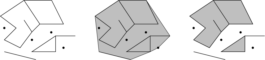
Figure 2. A PSLG, its convex hull and its polynomial hull.

A polygon or polygonal curve is a sequence of vertices $z_{1},\dots z_{n}$ and open edges $(z_{1},z_{2}),\dots,(z_{n},z_{1})$. A polygonal path or arc is a similar list of vertices, but with edges $(z_{1},z_{2}),\dots(z_{n-1},z_{n})$; the last is not connected back to the first. A polygon is simple if the vertices are all distinct and the edges are pairwise disjoint. A polygon is called edge-simple if the (open) edges are all pairwise disjoint, but vertices may be repeated.

The Jordan curve theorem implies that a simple closed polygon has two distinct complementary connected components, exactly one of which is bounded. This is the interior (or face) of the simple polygon. A domain (i.e., an open, connected set) that is the interior of some simple polygon will be called a simple polygonal domain. If $\Omega$ is multiply connected, but every connected component of $\partial\Omega$ is a simple polygon, we say $\Omega$ is a simple polygonal domain with holes. See Figure 3 for some examples.

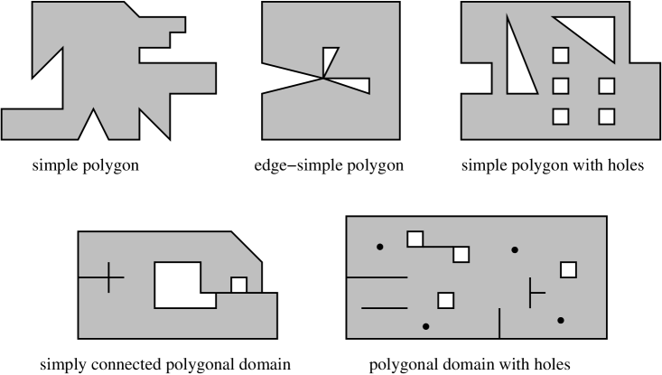
Figure 3. Examples of the different types of polygonal domains.

A triangle is a simple polygon with three vertices (hence three edges). We say a simple polygon $P$ has a triangular shape if there is a triangle $T$ so that $P$ is obtained by adding vertices to the edges of $T$. See Figure 4. Similarly, a quadrilateral $Q$ is a simple polygon with four vertices. We say a simple polygon $P$ has a quadrilateral shape (or is quad-shaped), if $P$ is obtained by extra adding vertices to the edges of a quadrilateral $Q$. The four vertices of $Q$ will be called the corners of $P$ (they are the only vertices of $P$ where the interior angle is not $180^{\circ}$). The other vertices of $P$ will be called interior edge vertices.

Figure 4. A triangle, a triangular shaped octagon, a quadrilateral and a quad-shaped decagon. The black dots are the corners and the white dots are the interior edge vertices.

A refinement (also called a sub-division) of a PSLG $\Gamma$ is a PSLG $\Gamma^{\prime}$ so that $V(\Gamma)\subset V(\Gamma^{\prime})$ and $\Gamma\subset\Gamma^{\prime}$. Informally, $\Gamma^{\prime}$ is obtained from $\Gamma$ by adding new vertices and edges and by subdividing existing edges. A mesh of $\Gamma$ is a sub-division $\Gamma^{\prime}$ of $\Gamma$ such that $\Gamma^{\prime}\subset{\rm{PH}}(\Gamma)$ and every face of $\Gamma^{\prime}$ is a simple polygonal domain. Note that we allow the addition of new vertices (called Steiner points) when we mesh a PSLG.

A mesh $\Gamma^{\prime}$ is called a triangulation if every face of $\Gamma^{\prime}$ is a triangle and is called a quadrilateral mesh or quad-mesh if every face is a quadrilateral. We will only consider meshes by convex quadrilaterals in this paper. It is always possible to triangulate a PSLG without adding Steiner points, but this is not the case for quadrilateral meshes. Sometimes we wish the mesh of a PSLG to cover the convex hull of the PSLG. In this case, we should add the boundary of the convex hull to the PSLG and mesh this new PSLG.

A quadrilateral dissection is a mesh in which every face is a quad-shaped polygon. (Similarly, a triangular dissection is a mesh where every face is triangular shaped, but we won’t use these in this paper.) More informally, a quadrilateral dissection is like a quadrilateral mesh, except that quadrilaterals whose boundaries intersect, do not have to intersect at just points or full edges; two edges can overlap without being equal and the corner of one piece can be an interior edge vertex of another piece. A vertex where this happens is called a non-conforming vertex. A quadrilateral dissection is also called a non-conforming quadrilateral mesh. See Figure 5.

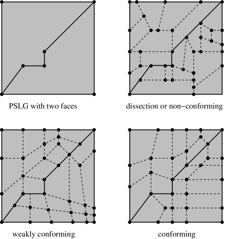
Figure 5. On the upper left is a PSLG with two simple polygonal faces, followed by a quadrilateral dissection, a weakly conforming quadrilateral mesh and a fully conforming quadrilateral mesh.

If every face of $\Gamma$ is a simple polygon, then a weak quadrilateral mesh of $\Gamma$ is a quadrilateral mesh of each face, without the requirement that the meshes match up across the edges of $\Gamma$. One of the main goals of this paper is to give a method of converting a weak mesh of a PSLG into a true mesh of similar size.

3. Connecting $\Gamma$ with no small angles

We reduce Theorem 1.1 to the case when every face of $\Gamma$ is a simple polygon.

Lemma 3.1.

If $\Gamma$ is a PSLG with $n$ vertices such that ${\rm{PH}}(\Gamma)$ is connected, then by adding at most $O(n)$ new edges and vertices, we can find a connected refinement $\Gamma^{\prime}$ of $\Gamma$ so that every face of $\Gamma^{\prime}$ is a simple polygon and any angles less than $60^{\circ}$ were already angles in a face of $\Gamma$.

Proof.

We use an idea of Bern, Mitchell and Ruppert [3] (refined by David Eppstein in [7]) of adding disks that connect different components of $\Gamma$. For each component $\gamma$ of $\Gamma$, except the component $\gamma_{u}$ (“u” for unbounded) bounding the unbounded complementary component of $\Gamma$, choose a left-most vertex $v$ of $\gamma$ and consider the left half-plane defined by the vertical line through this point, e.g., the vertical line on the left side of Figure 6. Consider the family of open disks in the left half-plane tangent to this line at $v$, and take the maximal open disk that does not intersect $\Gamma$. Its boundary must hit one or more components of $\Gamma$ that are distinct from $\gamma$. Choose one point on the circle from each distinct component (see the right side of Figure 6); a previously chosen disk touching some component counts as part of that component. Do this for each component of $\Gamma$ other than $\gamma_{u}$, taking the maximal open disk that is disjoint from $\Gamma$ and all the previously constructed disks.

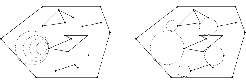
Figure 6. For each connected component of $\Gamma$ (except the component bounding the unbounded complementary component), choose the leftmost point and expand a disk until it contacts another component or a previously constructed disk. The process for one component is shown on the left; the result for all the components is shown on the right.

After all the disks have been placed, we connect the chosen points on the boundary of each disk by a PSLG inside the disk that has no angles $<60^{\circ}$, e.g., as illustrated in Figure 7. If the points are widely spaced, we can simply join them all to the origin (left side of Figure 7), assuming this does not form an angle $<60^{\circ}$. Otherwise we place a regular hexagon around the orgin and connect the points on the circle to the hexagon by radial segments (right side of Figure 7).

Figure 7. Joining points on a circle without creating angles $<60^{\circ}$.

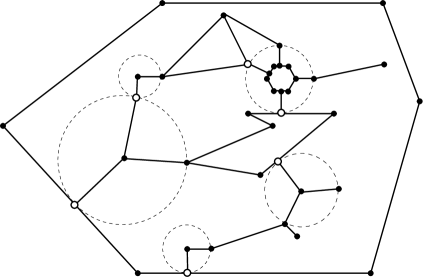
Figure 8. The PSLG in Figure 6 with the disks replaced by the connecting PSLGs from Figure 7. One face is not a simple polygon.

We have now replaced $\Gamma$ by another PSLG $\Gamma^{\prime}$ that is connected and contains no angles $<60^{\circ}$, except for those that were already in $\Gamma$. However, the faces of $\Gamma^{\prime}$ need not be simple polygons. We will add more disks to get this property.

Each face $\Omega$ of $\Gamma^{\prime}$ is either a simple polygon or $\partial\Omega$ has an edge or vertex whose removal disconnects $\partial\Omega$. If there is an edge $e$ so that $\partial\Omega\setminus e$ has two components, then one of them, $\gamma_{o}$ (“o” for outer) separates the other, $\gamma_{i}$ (“i” for inner) from $\infty$. Let $p$ be the endpoint of $e$ that meets $\gamma_{i}$; after a rotation and translation we can assume $p=0$ and $e$ lies on the negative real axis. Choose a vertex $v=a+ib$ on $\gamma_{i}$ that is farthest to the right, and consider disks in the half-plane $\{x+iy:x>a\}$ that are tangent to the vertical line $\{x+iy:x=a\}$ at $v$. There is a maximal such open disk $D$ contained in $\Omega$ and its boundary must intersect $\gamma_{o}$ or a previously generated disk. We repeat the process until there are no separating edges left and then connect points in the disks as above. The procedure is repeated at most once for each edge in the the boundary of the face, hence at most $O(n)$ edges and vertices are added.

Figure 9. If $\partial\Omega$ is not an edge-simple polygon then there is at least one edge $e$ that divides $\partial\Omega$ into “outer” and “inner” parts. The inner component can be connected to the outer component by adding a disk as described in the text.

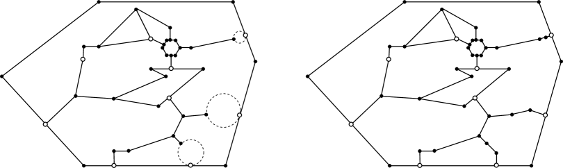
Figure 10. The PSLG in Figures 6 and 8 with the disks that prevent “two-sided” edges on the left and these disks replaced by PSLGs on the right. The resulting polygon has faces that are simple polygons.

We now have a PSLG so that all the faces are edge-simple. To make the faces simple, we choose a small circle around each repeated vertex and add polygonal arcs inscribed in arcs of these circles as shown in Figure 11. This is easy to do and the details are left to the reader. ∎

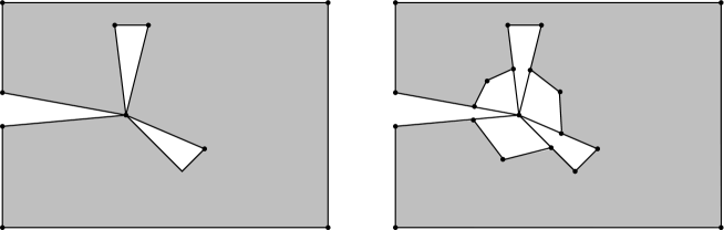
Figure 11. If there is a vertex that disconnects $\partial\Omega$, then we place cross-cuts around this vertex that block access from $\Omega$. These lie on some sufficiently small circle around the vertex and use at most $O(\deg(v))$ new edges and vertices. Summing over all vertices gives $O(n)$.

4. Propagation in quadrilateral meshes

In this section we review a few helpful properties of quadrilateral meshes.

Lemma 4.1.

If $\Omega$ is a simply connected polygonal domain that has a quadrilateral mesh, then the number of boundary vertices must be even.

Proof.

Let $Q$ be the number of quadrilaterals in the mesh, $I$ the number of interior vertices, $B$ the number of boundary vertices and $E$ the number of edges. Note that the number of edges on the boundary also equals $B$. Each quadrilateral has four edges, and each interior edge is counted twice, so $4Q=2(E-B)+B=2E-B.$ Thus $B=2(E-2Q)$ is even. ∎

Given a convex quadrilateral $Q$ with vertices ${a,b,c,d}$ (in the counterclockwise direction) and a point $x=ta+(1-t)b$, $0<t<1$, on the edge $[a,b]$, use a line segment to connect $x$ to $y=td+(1-t)c$ on the opposite edge of the quadrilateral. We will call this a propagation segment. By replacing $x$ with $y$ and repeating the construction, we create a path through the mesh that can be continued until it either hits a boundary edge or returns to the original starting point $x$. If $x$ is a boundary point, the latter is impossible, so the path must terminate at a distinct boundary point. Applying this to every midpoint of a boundary edge shows that each such edge is paired with a distinct edge, giving an alternate proof of Lemma 4.1.

We will repeatedly use propagation lines to subdivide a quadrilateral mesh, and so a basic fact we need is that this process preserves “niceness”.

Lemma 4.2 (Lemma 4.1, [4]).

Suppose $Q$ is a $\theta$-nice quadrilateral. If $Q$ is sub-divided by a propagation segment, then each of the resulting sub-quadrilaterals is also $\theta$-nice.

Corollary 4.3.

Suppose $\Omega$ is polygonal domain and every component of $\partial\Omega$ is a simple polygon. Then every nice quadrilateral mesh of $\Omega$ has a nice subdivision with exactly twice as many vertices on each component of $\partial\Omega$.

Proof.

Split each quadrilateral by two segments joining the midpoints of opposite sides. Each boundary edge is split in two so the number of boundary edges on each component doubles. ∎

Alternatively, one can just split each boundary edge into two, and propagate these vertices until they hit another boundary midpoint. See Figure 12 for an example of both types of subdivision.

               

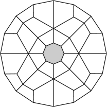
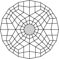
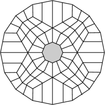
Figure 12. A mesh of an annular region (left) and its double (center). On the right we only double the boundary edges and propagate these.

Lemma 4.4.

A propagation path in a quadrilateral mesh can visit each quadrilateral at most twice (once connecting each pair of opposite sides)

Proof.

First we show each edge is visited at most once. Suppose the edge $e$ is visited twice by a path that crosses $e$ in the same direction both times. Then the path must cross $e$ at the same point both times (by the definition of how points propagate). Thus the path is really a closed loop that hits $e$ once. Next suppose $e$ is visited twice by a propagation path that crosses in opposite directions each time. Then there is another edge $f$, opposite to $e$ on one of the adjacent quadrilaterals, so that $f$ is crossed twice by the same path before $e$ is crossed twice. Iterating the argument gives a contradiction since the crossings of $e$ are separated by only a finite number of steps. Thus no edge is visited twice. Since each quadrilateral has four sides, and each side is visited at most once, each quadrilateral is visited at most twice. ∎

5. Sinks

We start by reviewing the definition given in the introduction, and then stating the results that we will prove in later sections.

We say that a mesh $\Gamma$ of the interior $\Omega$ of a simple polygon $P$ extends $P$ if $V(\Gamma)\cap P=V(P)$, i.e., the only vertices of the mesh that occur on $P$ are the vertices of $P$ (no extra boundary vertices are added).

As noted in the introduction, a sink is a simple polygon $P$ with the property that whenever we add an even number of vertices to the edges of $P$ to obtain a new polygon $P^{\prime}$, then there is nice mesh of the interior that extends $P^{\prime}$. By Lemma 4.1, a sink must have an even number of vertices and it is a simple exercise to check that neither a square nor a regular hexagon is a sink.

Lemma 5.1.

The regular octagon is a sink. If we add $M\geq 1$ vertices to the edges of a regular octagon $P$, the resulting polygon $P^{\prime}$ can be extended by a nice quadrilateral mesh with $O(M)$ elements.

From octagons we will construct other sinks, e.g. we can make a square into a sink by adding 24 vertices to its boundary, obtaining a 28-gon. Using such square sinks we can make any rectangle $R$ into a sink by adding $O({\mathcal{E}}(R))$ extra vertices to the sides of the rectangle (recall that for a quadrilateral $Q$, ${\mathcal{E}}(Q)\geq 1$ denotes its eccentricity, i.e., the longest side length of $Q$ divided by the shortest side length of $Q$). From the case of rectangles we will deduce:

Lemma 5.2.

If $Q$ is a nice quadrilateral, then we can make $Q$ into a sink $Q^{\prime}$ by adding $N=O({\mathcal{E}}(Q))$ vertices to the sides of $Q$. If we add $M$ vertices to the sides of $Q^{\prime}$, the resulting polygon $Q^{\prime\prime}$ can be extended by a nice mesh using $O(N+M^{2})$ quadrilaterals. More precisely, if $M=M_{1}+M_{2}$, where $M_{1}\geq 1$ is an upper bound for the number of extra points added to one pair of opposite sides of $Q$ and $M_{2}\geq 1$ is an upper bound for the number of extra points added to the other pair of opposite sides of $Q$ , then the number of elements in the nice extension of $Q^{\prime\prime}$ is $O(N+M_{1}M_{2})$.

In particular, if all the extra vertices are added to a single side of the quadrilateral $Q$ (or are only added to a single pair of opposite sides) then the number of mesh elements is $O(N+M)$.

In addition to the “regular” sinks described above, we will also need some “special” sinks that use some angles less than $60^{\circ}$. These sinks will be polygons inscribed in a circle or a sector. A cyclic polygon $P$ will refer to a simple polygon whose vertices $V$ are all on a circle that circumscribes the polygon. The polygon is $\theta$-cyclic if every complementary arc of $V$ on the circle has angle measure $\leq\theta$ (so the smaller $\theta$ is, the more $P$ looks like a circle).

In this paper, an $n$-tuple will always refer to an ordered list of $n$ distinct points on a circle, ordered counter-clockwise. Most commonly, we will take these on the unit circle $\circle{missing}\partial\mathbb{D}=\{z:|z|=1\}$ (a circle is a 1-dimensional torus, which is why the unit circle is traditionally denoted with a $\circle{missing}).An$(n,θ)$-tupleisan$n$-tuple$X ⊂

1. the vertices of $P$ contain $X$,

2. if we add vertices to the edges of $P$ to get a new polygon $P^{\prime}$, then there is quadrilateral mesh that extends $P^{\prime}$,

3. the edges of this mesh cover all the radial segments connecting the origin to points of $X$,

4. every angle in the mesh is between $60^{\circ}$ and $120^{\circ}$, except for any angles less than $60^{\circ}$ at the orgin formed by the radial segments corresponding to $X$; such angles remain undivided in the mesh.

This mesh actually conforms to the PSLG consisting of the closed radial segments connecting the origin to the points of $X$. We abuse notation slightly by saying it conforms to $X$. We will prove in Section 12 that

Lemma 5.3.

Given any $d$-tuple $X$ on the unit circle, there is a cyclic polygon $P$ with $O(d)$ vertices that is a sink conforming to $X$. If $M$ points are added to $P$, then the corresponding nice conforming mesh has at most $O(Md+d^{2})$ elements. For any $\theta>0$ the number of mesh elements that are not $\theta$-nice is $O(Md+d/\theta)$. If at most $O(K)$ extra points are added to each boundary edge of the sink, then at most $O(Kd/\theta)$ of the quadrilaterals are not $2\theta$-nice.

This lemma is the device that we will use in the proof of Theorem 1.1 to “protect” small angles in the original PSLG, i.e., to prevent these angles from being subdivided. When the vertex $v$ is on the boundary of a face of the PSLG, then instead of using the whole mesh we will only use the part that lies inside the face (a sector at $v$). This lemma is also one of two places where the worst case $O(n^{2})$ estimate comes from; the other is Theorem 13.1.

6. The regular octagon is a sink

In this section we prove Lemma 5.1. We start with:

Lemma 6.1.

Suppose $\theta_{1},\theta_{2},\theta_{3},\theta_{4}\in[0^{\circ},360^{\circ}]$, that $\theta_{1}<\theta_{3}$, $\theta_{2}<\theta_{4}$, and that

$$|\theta_{1}-\theta_{3}|,|\theta_{2}-\theta_{4}|<45^{\circ},\quad|\theta_{1}-\theta_{2}|,|\theta_{3}-\theta_{4}|<1^{\circ}.$$

Then the quadrilateral with vertices

$$z_{1}=e^{i\theta_{1}}=\cos(\theta_{1})+i\sin(\theta_{1}),\qquad z_{2}=2e^{i\theta_{2}}=2(\cos(\theta_{2})+i\sin(\theta_{2})),$$

$$z_{3}=e^{i\theta_{3}}=\cos(\theta_{3})+i\sin(\theta_{3}),\qquad z_{4}=2e^{i\theta_{4}}=2(\cos(\theta_{4})+i\sin(\theta_{4})),$$

has all its interior angles between $60^{\circ}$ and $120^{\circ}$. (Note that $z_{1},z_{3}$ are both on $\circle{missing}with$z_1$clockwisefrom$z_3$,and$z_2, z_4$areon$2

Proof.

This is a straightforward trigonometry calculation. We carry it out in detail for the corner located at $z_{1}$; the other three corners are very similar, and are left to the reader. The situation is illustrated in Figure 13. Consider the segments $[z_{1},z_{3}]$ and $[z_{1},z_{2}]$. The angle formed by these two sides at $z_{1}$ is the sum or difference of the angles that each of these sides makes with the radial line $L_{1}$ from the origin through $z_{1}$. Set $\tau=\theta_{3}-\theta_{1}$. Then considering the isosceles triangle formed by $0,z_{1},z_{3}$, we see that the angle between $[z_{1},z_{3}]$ and $L_{1}$ is between $90^{\circ}$ and $90^{\circ}+\tau/2$ (see Figure 13). Since $\tau\leq 45^{\circ}$, this is between $90^{\circ}$ and $112.5^{\circ}$.

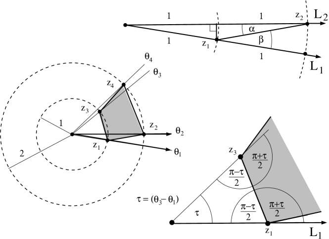
Figure 13. The diagram in the proof of Lemma 6.1. The quadrilateral formed by the points $z_{1},z_{2},z_{3},z_{4}$ has all four angles between $60^{\circ}$ and $120^{\circ}$ if $|\theta_{1}-\theta_{3}|,|\theta_{2}-\theta_{4}|$ are both smaller than $45^{\circ}$ and $|\theta_{1}-\theta_{2}|$, $|\theta_{3}-\theta_{4}|$ are both small enough, say less than $1^{\circ}$ (these numbers are not sharp).

On the other hand, if $\beta$ denotes the angle between $[z_{1},z_{2}]$ and $L_{1}$ (as labeled in Figure 13) and $\alpha$ denotes the angle formed by $[z_{1},z_{2}]$ and the ray $L_{2}$ from $0$ through $z_{2}$, then $\beta=(\theta_{2}-\theta_{1})+\alpha$. We claim $\alpha\leq\theta_{2}-\theta_{1}$. To prove this, consider the segment perpendicular to $[0,z_{2}]$ through $z_{1}$. This intersects $[0,z_{2}]$ closer to $0$ than to $z_{2}$ (see Figure 13) and hence $\tan(\alpha)\leq\tan(\theta_{2}-\theta_{1})$, giving the claimed inequality. Thus

$$\beta=|\theta_{2}-\theta_{1}|+\alpha\leq 2|\theta_{2}-\theta_{1}|\leq 2^{\circ}.$$

This proves the angle bounds at $z_{1}$ with room to spare. The argument for $z_{3}$ is identical and the arguments for $z_{2}$, $z_{4}$ are almost the same (we only need to estimate $\alpha$, not $\beta$). ∎

Lemma 6.2.

Suppose $\theta>0$ and that ${\bf z}=\{z_{1},\dots,z_{n}\}$ and ${\bf w}=\{w_{1},\dots,w_{n}\}$ are both $(n,\theta)$-tuples on the unit circle (in particular, they are both ordered on the circle in the same direction). Given any $\tau>0$ there is an integer $t$ (depending on $\tau$, but not on ${\bf z}$ or ${\bf w}$) and a sequence of $(n,\theta)$-tuples $\{z_{1}^{k},\dots,z_{n}^{k}\}_{k=1}^{t}$ so that $z_{j}^{0}=z_{j}$ and $z_{j}^{t}=w_{j}$ for $j=1,\dots n$ and so that $|z_{j}^{k}-z_{j}^{k+1}|<\tau$ for all $k=0,\dots,t-1$ and $0=1,\dots n$. In other words, we can discretely deform ${\bf z}$ into ${\bf w}$ through a sequence of $(n,\theta)$-tuples that move individual points by less than $\tau$ at each step. If $z_{j}=w_{j}$ for some $j$, then the points $z_{j}^{k}$, $k=1,\dots t$ are all the same.

Proof.

Choose arguments $\theta_{1},\phi_{1}\in(0^{\circ},360^{\circ}]$ for $z_{1}$ and $w_{1}$. Then choose arguments $\{\theta_{j}\}_{2}^{n}$ for $z_{2},\dots z_{n}$ in $(\theta_{1},\theta_{1}+360^{\circ})$; note that the arguments increase since we assume the $n$-tuple ${\bf z}$ is ordered in the counter-clockwise direction. Similarly choose arguments $\{\phi_{j}\}_{2}^{n}\subset(\phi_{1},\phi_{1}+360^{\circ})$ for the elements of ${\bf w}$. Now use linear interpolation on the angles, i.e.,

$$\theta_{j}^{k}=(1-\frac{k}{t})\theta_{j}+\frac{k}{t}\phi_{j},\qquad k=0,\dots,t,$$

to define points $z_{j}^{k}=\exp(i\theta_{j}^{k})$. See Figure 14. Since both $n$-tuples have the same orderings, none of the lines in Figure 14 cross each other, hence these intermediate points define $n$-tuples with the correct ordering. Moreover, the $0\leq\arg(z_{k}^{j})-\arg(z_{k}^{j+1})<360^{\circ}/t$ is as small as we wish if $t$ is large enough. In particular, it is smaller than $\tau$ if $t$ is large enough, depending only on $\tau$. ∎

Figure 14. Linear interpolation of the arguments ($n=7$, $t=10$).

Corollary 6.3.

Suppose that ${\bf z}=\{z_{1},\dots,z_{n}\}$ and ${\bf w}=\{w_{1},\dots,w_{n}\}$ are $(n,45^{\circ})$-tuples. There is an integer $s$ so that the annular region bounded between $P_{\bf z}$ and $2^{-s}P_{\bf w}$ can be meshed with $ns$ quadrilaterals using only angles between $60^{\circ}$ and $120^{\circ}$. (Recall that $P_{\bf z}$ is a cyclic polygon inscribed on the unit circle $\circle{missing},and$2^-sP_w$isacyclicpolygoninscribedon$2^-s

Proof.

This is immediate from Lemma 6.1 and Lemma 6.2. See Figure 15. ∎

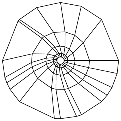
Figure 15. A quadrilateral mesh of the annular region bounded by two $20$-gons inscribed on concentric circles (the outer $20$-tuple is a regular octagon with 12 randomly chosen points added; the inner one is a regular icosagon). This illustrates Corollary 6.3

Lemma 6.4.

Suppose ${\bf z}=\{z_{1},\dots,z_{n}\}$ is an $(n,45^{\circ})$-tuple on the unit circle and suppose $V$ is a set of $t$ points on the edges of the inscribed polygon $P_{\bf z}$ corresponding to ${\bf z}$. Let ${\bf w}$ be the $(n+t)$-tuple consisting of ${\bf z}$ and the radial projection of $V$ onto the unit circle. Let $A$ be the annular region bounded between $P_{\bf z}$ and $\frac{1}{2}P_{\bf w}$ and consider the quadrilateral mesh formed by joining each point of $\frac{1}{2}{\bf w}\subset\{|z|=1/2\}$ to its radial projection onto $P_{\bf z}$. Then all angles used in this mesh are between $67.5^{\circ}$ and $112.5^{\circ}$.

Proof.

Each angle on $\frac{1}{2}P_{\bf w}$ is the supplement of the base angle of an isosceles triangle with vertex at the origin and vertex angle $\leq 45^{\circ}$, hence is between $90^{\circ}$ and $112.5^{\circ}$. Each angle on $P_{\bf z}$ is clearly between $67.5^{\circ}$ and $112.5^{\circ}$. See Figure 16. (The figure shows ${\bf z}$ as a regular octagon, but this need not be the case in general.) ∎

Figure 16. The annular region between a octagon with four extra points added to the sides and the “rounded” version of this polygon. Since $\theta\leq 45^{\circ}$, we have $\alpha=90^{\circ}-\theta/2$ is between $67.5^{\circ}$ and $90^{\circ}$. Similarly $67.5^{\circ}\leq\alpha\leq\beta\leq 180^{\circ}-\alpha\leq 112.5^{\circ}$. Finally, $90^{\circ}\geq\gamma\geq 90^{\circ}-\theta/2\geq 67.5^{\circ}$ as claimed in the text.

Lemma 6.5.

Suppose $P$ is a regular octagon, centered at the origin with four of its vertices on the coordinate axes. Nicely mesh the interior using twelve quadrilaterals, as shown in Figure 17. Place $t$ distinct points on the sides of octagon that touch the $x$-axis, and connect each of these to another boundary point by a propagation path in the given mesh of the octagon. The resulting refinement is a nice mesh with at most $12+4t$ elements.

Proof.

The niceness is immediate from Lemma 4.2. The complexity bound follows from the fact that the propagation paths don’t intersect unless they agree (i.e., two of the points are endpoints of the same path), and each passes through four mesh elements. See Figure 17. ∎

     

Figure 17. On the left is the “standard mesh” of a regular octagon. In the center is a mesh formed by non-intersecting propagation paths; given $t$ extra points, $4t$ new elements are created. In general, $\simeq t^{2}$ new elements might be formed (right side) by intersecting propagation paths.

Lemma 6.6.

Suppose ${\bf z}$ is an $(n,45^{\circ})$-tuple on the unit circle and $P$ is the cyclic polygon with these vertices. Suppose we form a new polygon $P^{\prime}$ by adding $k$ distinct points to $P$ (all distinct from ${\bf z}$), so that $n+k$ is even. Then $P^{\prime}$ has a nice mesh with $O(n+k)$ elements. In particular, this holds if $P$ is a regular octagon, so this result contains Lemma 5.1 as a special case.

Proof.

Let ${\bf z^{\prime\prime}}$ be the radial projection of ${\bf z}$ onto $\frac{1}{2}\circle{missing}\{|z|=\frac{1}{2}\}$ and let $P^{\prime\prime}$ be the cyclic polygon with these vertices. Clearly $n\geq 8$, so $n+k\geq 8$. Hence $n+k=n+2t$ for some $t\geq 0$. Let ${\bf w}$ be some $(8+2t)$-tuple as described in Lemma 6.5: eight points are evenly spaced on the unit circle and the other $2t$ are the endpoints of $t$ non-intersecting propagation paths for the standard mesh of the octagon shown in Figure 17. Let $s$ be the constant from Corollary 6.3. Let $P_{\bf w}$ be the cyclic polygon on $\circle{missing}withvertices$w$andlet$2^-s-1 P_w$bethedilationofthisbyafactorof$2^-s-1$(soitisacyclicpolygonon$2^-s-1

Nicely mesh $2^{-s-1}P_{\bf w}$ by cutting the standard mesh of the octagon by the $t$ propagation paths as in Lemma 6.5. Let ${\bf z^{\prime\prime}}$ be the rounded version of ${\bf z^{\prime}}$. Apply Lemma 6.3 to nicely mesh the region between $2^{-s-1}P_{\bf w}$ and $\frac{1}{2}P_{\bf z^{\prime\prime}}$. Then use Lemma 6.4 to nicely mesh the region between $\frac{1}{2}P_{\bf z^{\prime\prime}}$ and $P^{\prime}$. Thus the $P^{\prime}$ has been nicely meshed without adding any extra boundary points, as claimed. See Figure 18 (but note that scales are distorted in this figure to make the smaller layers more visible). ∎

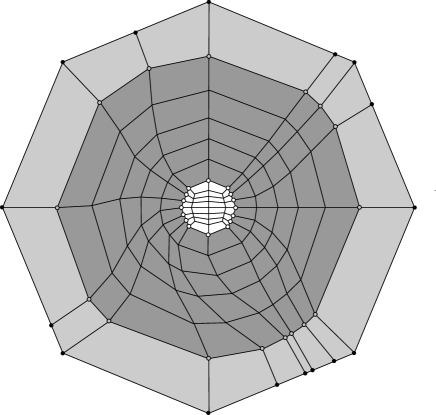
Figure 18. This illustrates the proof of Lemma 6.6 with $n=8,k=8,t=4,s=5$. The back dots are ${\bf z^{\prime}}$, the gray dots are $\frac{1}{2}{\bf z^{\prime\prime}}$ and the white dots are $2^{-s-1}{\bf w}$. The light gray region is meshed by Lemma 6.4, the dark gray by Corollary 6.3 and the white by Lemma 6.5. These results ensure the angles in each region satisfy the desired bounds. Note that the cyclic polygons should be inscribed on circles with radii $1,\frac{1}{2},\dots,\frac{1}{32}$, but to make the combinatorics more visible we have made the circles larger than this (which distorts the angles).

7. Square shaped sinks

Given octagonal sinks, we can build sinks with other shapes. In this section we show that there are “square shaped sinks”:

Lemma 7.1.

We can add 24 vertices to the sides of a square $S$ to make it into a sink. If we then add $2M>0$ extra vertices to the sides of the sink, the interior can be re-meshed using $O(M^{2})$ nice quadrilaterals. If at most $M_{1}\geq 1$ points are added to one pair of opposite sides of $S$, and at most $M_{2}\geq 1$ are added points are added to the other pair of opposite sides, then the number of quadrilaterals needed is $O(M_{1}M_{2})$.

Proof.

We want to place a copy of a regular octagon inside a square in a certain way. Suppose we have a octagon centered at the origin, with sides of length 1 and two sides parallel to each coordinate axis. Let $a$ denote the origin. Let $b=(\frac{1}{2}+\frac{1}{\sqrt{2}},\frac{1}{2}),$ and $c=(\frac{1}{2},\frac{1}{2}+\frac{1}{\sqrt{2}})$ be the vertices of the octagon in the first quadrant. See Figure 19. Now form an equilateral triangle $T$ with one side parallel to the $x$-axis and passing through $b$, the vertex $e$ opposite this side on the same vertical line as $b$, and a side passing from $e$ through $c$ ($T$ is the dashed triangle in Figure 19). Let $d$ be the vertex of the triangle inside the octagon. Let $f$ be the third vertex of the triangle. Let $S$ be the axis-parallel square centered at the origin and passing through $e$.

Figure 19. Placing the octagon within a concentric square.

The Law of Sines implies that

$$|f-b|=|d-b|=|b-c|\frac{\sin 75^{\circ}}{\sin 60^{\circ}}=1\cdot\frac{1+\sqrt{3}}{\sqrt{6}}\approx 1.11536,$$

and hence

$$|e-b|=|d-b|\tan 60^{\circ}=\frac{1+\sqrt{3}}{\sqrt{2}}\approx 1.93185.$$

Therefore

$$e=(\frac{1}{2}+\frac{1}{\sqrt{2}},\frac{1}{2}+\frac{1+\sqrt{3}}{\sqrt{2}})\approx(1.20711,2.43185),$$

and

$$f=(\frac{1}{2}+\frac{1}{\sqrt{2}}+\frac{1+\sqrt{3}}{\sqrt{6}},\frac{1}{2})\approx(2.32246,.5).$$

Hence $f$ is inside the square $S$. Therefore the line through $a$ and $b$ intersects the segment $[e,f]$ at a point $g$ strictly inside the square, as shown in Figure 19.

We now mesh the region between the square and the octagon as in Figure 20.

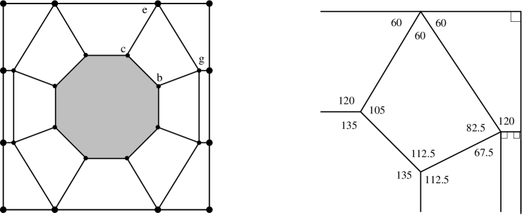
Figure 20. The mesh of the region between the octagon and the square using the points defined in the text. The mesh is symmetric with respect to the $x$ and $y$ axes, so it suffices the check the angles in the upper right corner, as done in the right side of the figure.

Consider boundary points of the square that propagate through this mesh. See Figure 21. Every point on the two vertical sides of the square hits the octagon under propagation, and this is true for some points on the horizontal sides of the square, but there are some points that propagate to the other side of the square without hitting the octagon (e.g., the dashed line on the far right in Figure 21).

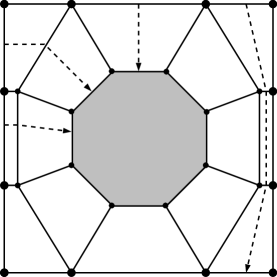
Figure 21. Some boundary points propagate to the octagon, but other propagate past it.

To fix this, we place two small squares inside $S$ as shown in Figure 22. Inside each square we place an octagon and mesh the region between the small square and the small octagon as shown in Figure 19, but rotated by $90^{\circ}$, so that every propagation path hitting the small square from above or below propagates to the small octagon inside it. Paths hitting the small square on the vertical sides either propagate to the small octagon, or past it and then to the large octagon. In either case, every boundary point of the large square $S$ now propagates to one of the three octagons.

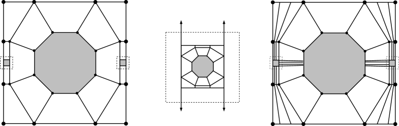
Figure 22. Now all boundary points of the square propagate to one of three octagons inside the square. After re-meshing to account for the new vertices on the small squares, the mesh has 28 vertices on the boundary of the large square.

If we add an even number of new vertices to the boundary of the large square, we can propagate these until they each hit one of the three octagons. If each octagon gets an even number of points, then, since each octagon is a sink, we can re-mesh the interior of the octagons using these points and without adding any new points to the boundaries of the octagons. If some octagon gets an odd number of extra points, then exactly two of them do. If these two are the central octagon and one of the smaller side octagons, we connect them a propagation path, thus adding one more point to each boundary. If the two side octagons have an odd number of extra points each, then we connect them both to the central octagon by a propagation path; this adds one point to each of the smaller octagons and adds two points to the central octagon. In either case, all three octagons now have an even number of boundary points and we can proceed as before. This proves a square can be turned into a sink; counting points in Figure 22 shows that the sink has seven edges on each side of the original square, hence it has 28 vertices in all (including the corners of the square).

If we add $M>0$ points to the boundary of the square, and propagate these points until they hit one of the three octagons, then $M$ points are created on the boundaries of the octagons. After add extra paths (for parity) and re-mesh the octagons, $O(M)$ quadrilaterals are created inside the octagons. However, up to $O(M^{2})$ elements might be formed between the octagons and the boundary of the square. For example, if $M_{1},M_{2}\geq 1$ points are added to two edges that are both adjacent to the same corner of the square $S$, then the every propagation path from one group crosses every path from the other group, generating $M_{1}\cdot M_{2}$ quadrilaterals. See Figure 23. This can only happen when extra points are added to adjacent sides of $S$; if all the extra points are added to one side, or to a single pair of opposite sides of $S$, then only $O(M)$ quadrilaterals are needed to re-mesh the interior of $S$. ∎

Figure 23. $M_{1},M_{2}$ extra points placed on two edges adjacent to a corner of a square sink can create $M_{1}\cdot M_{2}$ mesh elements.

8. Rectangular Sinks

Let $\lceil x\rceil=\min\{n\in\mathbb{Z}:n\geq x\}$.

Lemma 8.1.

For any rectangle $R$ we can add at most $28\cdot\lceil{\mathcal{E}}(R)\rceil$ vertices to the boundary and make $R$ into a sink. If we then add $M_{1}\geq 1$ extra vertices to one pair of opposite sides, and add $M_{2}\geq 1$ extra vertices to the other pair of opposite sides, then the interior can be re-meshed using $O({\mathcal{E}}(R)+M_{1}M_{2})$ nice quadrilaterals.

Proof.

The idea for this proof was suggested by one of the referees and modifies an earlier proof of the author.

We claim the construction of square sinks in the previous section can be adapted to also handle rectangles with ${\mathcal{E}}(R)\leq\sqrt{2}$. See Figure 24. This figure replicates the left side of Figure 22 and shows that if the two vertical sides of the square are moved outward and the small shaded squares are expanded accordingly, the same construction gives a rectangular sink. This works as long as the expanding shaded squares do not cover the point $g$. This holds as long as $\Re(p)-\Re(g)\leq 2\Im(g)$ ($\Re$ and $\Im$ denote the real and imaginary parts of a complex number).

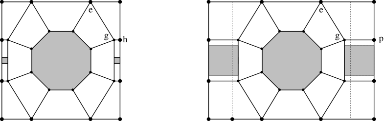
Figure 24. The construction for squares also works for rectangles with eccentricity sufficiently close to $1$. The left side is the same as in Figure 22. The right side is obtained by moving the vertical sides of the big square outwards and expanding the small shaded squares as shown (we also expand the mesh inside these squares accordingly).

Using the formulas from Section 7 we can show that

$$|b-f| = (1+\sqrt{3})/\sqrt{6}\approx 1.11536,$$

$$|b-g| = |b-f|\sin 60^{\circ}/\sin 97.5^{\circ}\approx.974261,$$

$$\Re(g) = \Re(b)+|b-g|\cos 22.5^{\circ}\approx 2.10721,$$

$$\Im(g) = \Im(b)+|b-g|\sin 22.5^{\circ}\approx.872833.$$

These estimates imply $A=\Re(g)+2\Im(g)\approx 3.85287$. Since $\Im(e)\approx 2.43185$, this says the construction works for rectangles with eccentricity up to $A/\Im(e)\approx 1.58434$. This number is larger that $\sqrt{2}\approx 1.41421$, proving the claim.

It is not hard to see that a $1\times r$ rectangle can be sub-divided into at most $\lceil r\rceil$ rectangles with eccentricity in $[1,\sqrt{2}]$ (it suffices to consider $1<r<2$ and note that a $1\times\sqrt{2}$ rectangle can be split into two $1\times\frac{1}{\sqrt{2}}$ rectangles that also have eccentricity $\sqrt{2}$). Therefore we can place a modified square sink in each sub-rectangle. When we add new boundary points to the large rectangle, every such point is on the boundary of one of the sub-rectangles. If every sub-rectangle gets an even number of boundary points, we simply re-mesh all the rectangular sinks. Otherwise, we can add points to the common sides of the sub-rectangles so that they all end up with an even number of new points (see Figure 25) and then re-mesh.

Figure 25. Any $1\times r$ rectangle can be sub-divided into at most $\lceil r\rceil$ sub-rectangles with eccentricity bounded by $\sqrt{2}$, and each such sub-rectangle is a sink. When we add extra boundary points, it is easy to add internal points to make sure each sub-rectangle ends up with an even number of boundary points. Then each can be re-meshed.

The bound on the number of mesh elements needed when we add extra boundary points follows immediately from the similar bounds for the square and near-square sub-sinks. ∎

9. Nice quadrilateral sinks

Finally, we are ready to prove Lemma 5.2 (nice quadrilateral sinks exist).

Proof of Lemma 5.2.

As shown in Figure 26, we can mesh a nice quadrilateral $Q$ using nine elements, four of which are rectangles, each rectangle touching one side of $Q$ and with the sides of the rectangle parallel or perpendicular to that side of $Q$. It is easy to check that each of the five remaining regions is $\theta$-nice if $Q$ is $\theta$-nice. It is also easy to see that we can choose the rectangles with eccentricity bounded by $O({\mathcal{E}}(Q))$.

    

Figure 26. The nice quadrilateral $Q$ (left) is meshed with 4 rectangles (shaded) and 5 smaller quadrilaterals (white). Every boundary point of $Q$ is either on one of the rectangles, or it propagates through one of the white corner quadrilaterals to a rectangle.

When we place extra points on the boundary of $Q$, each point is either on the side of a rectangle or on the boundary of one of the four corner regions. In the latter case, we propagate the point through the corner to a rectangle. If every rectangle ends up with an even number of the new boundary points, then we can re-mesh each rectangle since they are all sinks. Otherwise, either all four rectangles get an odd number of boundary points, or exactly two do. In the first case, we can connect opposite sides by a propagation segment as shown on the top right of Figure 27. If exactly two rectangles get an odd number of boundary points, and these two rectangles touch opposite sides of $Q$, then we again connect them by a propagation segment as shown on the top left in Figure 27.

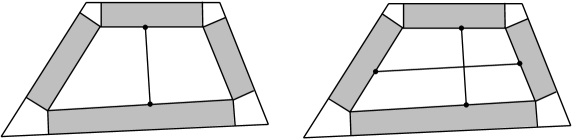
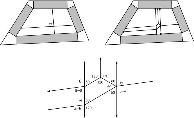
Figure 27. The top figures show what to do if opposite pairs of rectangles get an odd number of new boundary points: we connect the pair by a propagation segment to make the number of boundary points even again. The second row shows the construction when a pair of adjacent rectangles each get an odd number of extra boundary points. The bottom figure verifies the necessary angle bounds.

The final possibility is that exactly two rectangles get an odd number of new boundary points and these rectangles touch adjacent sides of $Q$. In this case, we make a connection as shown in the middle of Figure 27. Here we connect both pairs of opposite rectangles by propagation segments for $Q$, and these segments must cross at some angle $\theta$ that is between $60^{\circ}$ and $120^{\circ}$. We then replace these segments by parallel segments as shown in Figure 27. The exact angles near the crossing point are show in the lower part of Figure 27. These angles are all between $60^{\circ}$ and $120^{\circ}$. After adding these segments, all the rectangles have an even number of new boundary points and they can then be re-meshed. Thus the quadrilateral with the extra $O({\mathcal{E}}(Q))$ boundary points due to the four rectangular sinks is also a sink.

As with square sinks and rectangular sinks, certain placements of $M$ extra points near the corners of $Q$ can create $\simeq M^{2}$ quadrilaterals in the “corner sub-regions” of $Q$. However, if we place at most $M_{1}\geq 1$ points on one pair of opposite sides of $Q$, and at most $M_{2}\geq 1$ points on the other pair of opposite sides, then each of the four sub-rectangles gets (either directly or by propagation through a corner region) at most $M_{1}$ points on one pair of opposite sides and $M_{2}$ points on the other pair of opposite sides. Thus the sink can be re-meshed using $O({\mathcal{E}}(Q)+M_{1}M_{2})$ elements. ∎

10. The standard sector mesh

A sector of angle $\theta$ and radius $r$ is a region in the plane isometric to

$$S=\{z=te^{i\psi}:0<t<r,|\psi|<\theta/2\}.$$

The point corresponding to the origin is called the vertex of the sector. We shall use the term “inscribed sector” to refer to polygons where the circular arc in $S$ has been replaced by a polygonal arc with the same endpoints and possibly other vertices placed (in order) along the circular arc. See Figure 28. A “truncated sector” with inner radius $r_{1}$ and outer radius $r_{2}$ is a region similar to

$$S=\{z=te^{i\psi}:r_{1}<t<r_{2},|\psi|<\theta/2\},$$

and we define an inscribed truncated sector in the analogous way. See Figure 28.

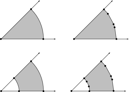
Figure 28. The definition of a sector and truncated sector (left top and bottom) and inscribed sector and inscribed truncated sector (right top and bottom).

Given a sector of angle $\theta\leq 120^{\circ}$, the “standard sector mesh” is illustrated in Figure 29. Note that every angle (except possibly the angle $\theta$ at the vertex of the sector), is between $60^{\circ}$ and $120^{\circ}$. This can be verified by the following calculations ($\theta_{1}$, $\theta_{2}$ are as labeled in Figure 29):

$$0<\theta\leq 120$$

$$60\leq\theta_{1}=180-60-\frac{1}{2}\theta\leq 120$$

$$60\leq\theta_{2}=\frac{1}{2}(180-\frac{1}{2}\theta)\leq 90$$

Note that the mesh covers an inscribed sector, where the circular arc is replaced by a polygonal arc with two segments of equal length.

Figure 29. The standard sector mesh. If $0<\theta\leq 120^{\circ}$ this uses only angles between $60^{\circ}$ and $120^{\circ}$, except possibly for the angle $\theta$ at the vertex of the sector.

We define a similar, but more complicated “standard mesh” of a truncated sector as is illustrated in Figure 30. Here we assume $0^{\circ}<\theta\leq 60^{\circ}$. In the figure, we take the vertex of the sector to be the origin, one radial edge along the positive real axis and the other along the ray passing through $0$ and $e^{i\theta}$. Define the points

$$z_{1}=1,z_{2},=2,z_{3}=4,z_{4}=8,z_{5}=e^{i\theta},$$

$$z_{8}=4e^{i\theta},z_{9}=8e^{i\theta},z_{10}=8e^{i\theta/2},z_{11}=\frac{3}{4}z_{3}+\frac{1}{4}z_{8}.$$

The point $z_{12}$ is the intersection of the horizontal line through $z_{11}$ and the line of slope $\sqrt{3}$ through $z_{2}$. The point $z_{6}$ is the intersection of the upper radial edge of the sector with the line of slope $-\sqrt{3}$, through $z_{2}$. The point $z_{7}$ is the intersection of the same radial edge of the sector with the line of slope $-\sqrt{3}$ through $z_{12}$.

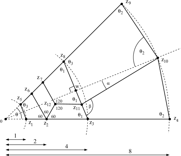
Figure 30. The standard truncated sector mesh. Angle bounds are given in the text.

It is easy to check that $\theta\leq 60^{\circ}$ implies

$$60^{\circ}\leq\theta_{1}=90^{\circ}-\theta/2\leq 90^{\circ},$$

$$75^{\circ}\leq\theta_{2}=90^{\circ}-\theta/4\leq 90^{\circ},$$

$$90^{\circ}\leq\theta_{3}=180^{\circ}-\theta_{1}=90^{\circ}+\theta/2\leq 120^{\circ}.$$

From the diagram, we also see that if $w$ is the intersection of the segments $[z_{3},z_{8}]$ and $[0,z_{10}]$, then

$$\tan\alpha=\frac{|w-z_{11}|}{|w-z_{10}|}=\frac{|w-z_{3}|/2}{|z_{10}|-|w|}=\frac{(|z_{3}|/2)\sin\frac{\theta}{2}}{8-|z_{3}|\cos\frac{\theta}{2}}=\frac{2\sin\frac{\theta}{2}}{8-4\cos\frac{\theta}{2}}.$$

Since $\theta/2\leq 30^{\circ}$, this means

$$\tan\alpha\leq\frac{1}{2(4-\sqrt{3})}\approx.220463<.267949\approx 2-\sqrt{3}=\tan 15^{\circ}.$$

Thus $0\leq\alpha\leq 15^{\circ}$. Hence the two angles at $z_{10}$ are $\theta_{2}\pm\alpha$, and satisfy

$$75^{\circ}\leq\theta_{2}\pm\alpha=(90^{\circ}-\frac{\theta}{4})\pm\alpha\leq 105^{\circ}.$$

Therefore

$$\beta = 360^{\circ}-\theta_{2}-(180^{\circ}-\theta_{1})-(\theta_{2}-\alpha)$$

$$= 180^{\circ}-2\theta_{2}+\theta_{1}+\alpha$$

$$= 180^{\circ}-(180^{\circ}-\theta/2)+(180^{\circ}-\theta)/2+\alpha$$

$$= 90^{\circ}+\alpha,$$

so $90^{\circ}\leq\beta\leq 90^{\circ}+15^{\circ}\leq 105^{\circ}.$ Clearly, the supplementary angle to $\beta$ also satisfies the desired bounds. Finally, we should check that the point $z_{12}$ is actually in the lower half of the sector as shown in Figure 30. Note that

$$\Im(z_{12})=\Im(z_{11})\leq|z_{3}-z_{11}|=\frac{1}{2}|z_{3}|\sin\frac{\theta}{2}\leq 2\tan\frac{\theta}{2},$$

and the right hand side is the length of the vertical segment connecting $z_{2}$ to the segment $[0,z_{10}]$ (the dashed ray in Figure 30). Since $\Re(z_{12})>\Re(z_{2})$, this implies $z_{12}$ is below the dashed line, as claimed.

11. Layered sector meshes

In this section we combine the standard meshes for a sector and truncated sector to form a “layered” sector mesh.

First consider two line segments that meet at angle $\theta\leq 120^{\circ}$. Without loss of generality we can assume these are the radial segments $[0,1]$ and $[0,e^{i\theta}]$. Mesh the sector of radius 1 between these lines using the standard sector mesh. Then mesh the truncated sector between $[1,8]$ and $[e^{i\theta/2},8e^{i\theta/2}]$ using the standard truncated sector mesh. Then reflect this mesh over the segment $[0,8e^{\theta/2}]$. The union of these three components gives a 2-layer mesh of the sector of angle $\theta$. The important point is that the vertices on the radial edges of the sector are at radii that are independent of the angle of the sector. Therefore, if we mesh disjoint sectors at the same vertex that share a radial edge, then the meshes match up along that radial edge. See Figures 31 and 32.

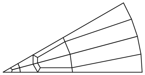
Figure 31. A 2-layer sector mesh. At the vertex of the sector is the standard sector mesh, and between radii 1 and 8 are two copies of the standard truncated sector mesh for angle $\theta/2$ (they are symmetric with respect to the sector bisector).

      

      

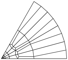
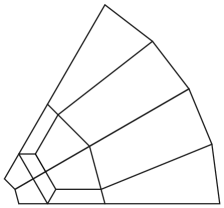
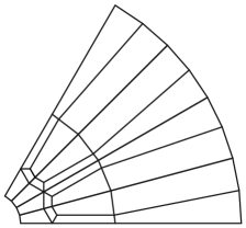
Figure 32. A 3-layer sector mesh. The upper left shows a sector mesh with three layers and the other three pictures show rescalings of each layer. At top right is layer 1, the standard sector mesh for some angle $\theta$ (this layer is not visible in the picture at upper left); at lower left is layer 2, two copies of a standard truncated sector mesh for angle $\theta/2$; and at lower right is layer 3, four copies of a standard truncated mesh for angle $\theta/4$. More layers could be added to give as many points as desired on the outer boundary of the sector (the number of such points doubles with each layer).

By repeating the construction on larger truncated sectors we can bisect each of these angles again, and continue until the angles are as small as we wish. If we start with an $n$-tuple $X=X^{0}$ on the unit circle, the standard mesh in each sector creates a mesh of the cyclic polygon with vertices $X^{1}$. Using a pair of symmetric truncated sector meshes as above, we quad-mesh the region between the cyclic polygon for $\frac{1}{8}X^{1}$ and $X^{2}$. In general, using $k$ layers we can mesh the cyclic polygon for $X^{k}$ (this was defined in Section 5, by repeatedly bisecting the components of $\circle{missing}X$).

Figure 33. Meshing each sector using two layers as described in Section 11 gives a conforming mesh of the PSLG consisting of six line segments meeting at a point.

We now do a similar construction in each given sector. See Figure 33 for an example of a two layer mesh in six sectors. The mesh points that occur on the given segments occur at fixed distances from the origin, independent of the angle, so the sector meshes fit together to form a mesh of a polygon inscribed in the circle. We summarize our conclusions as:

Lemma 11.1.

Given any $(d,120^{\circ})$-tuple $X$ on the circle and a non-negative integer $k$, there is a nice conforming quadrilateral mesh for $X^{k}$ that uses $O(2^{k}d)$ elements and so that the edges of the mesh cover each radial segment connecting the orgin to a point of $X$.

This mesh will form the center part of the protecting sinks constructed next.

12. Sinks protecting a vertex

Proof of Lemma 5.3.

Consider $d$ segments meeting at a single point, as shown on the left side of Figure 34. Assume the meeting point is the origin and the segments all have length $1$. If any of the angles formed are $\geq 45^{\circ}$ then we add extra radial segments until all the angles are $\leq 45^{\circ}$ (the dashed lines in the top left of Figure 34). When finished, we have $d+O(1)=O(d)$ segments.

Figure 34. The construction of a vertex protecting sink. We first add edges so every sector has angle $\leq 45^{\circ}$ (upper left). When then create cyclic polygons $P$ and $\frac{1}{2}P$ (upper right) and place bounded eccentricity quadrilaterals $\{Q_{j}\}$ between these polygons (shaded region in lower left picture). We then propagate the corners of these quadrilaterals until they run into another quadrilateral (bottom right). Inside a much smaller polygon (dark gray, lower right) we place the layered sector mesh given by Lemma 11.1. The white annular region between this and $\frac{1}{2}P$ is meshed using Corollary 6.3. We show the case when the sink surrounds the vertex $v$, but if $v$ is on the boundary of a face of the PSLG, then the picture above may be restricted to the sector with vertex $v$ that lies inside the face.

Intersect the radial segments with the circles of radii $1$ and $\frac{1}{2}$ centered at the origin, and inscribe cyclic polygons $P$ and $\frac{1}{2}P$ on each circle using these points. Let $A$ be the topological annulus bounded by these two polygons. The edges of $A$ on $\frac{1}{2}P$ will be called the inner edges and the opposite sides on $P$ will be called the outer edges; these outer edges will be the boundary edges of the sink.

Place quadrilaterals $\{Q_{j}\}$ in $A$ as shown by the shaded regions on the bottom, left of Figure 34. Each quadrilateral has one side that is an inner side of $A$ and two sides that are sub-segments of the radial segments. The fourth side is parallel to the first and chosen so that the quadrilateral has bounded eccentricity (for large angles, the fourth side might be a side of $P$, but for small angles it is in the interior of $A$. Later, it will be convenient to assume the radial sides of the quadrilaterals $\{Q_{j}\}$ only take certain values, e.g., powers of $2$. This is easy to do while keeping bounded eccentricity.

Next, propagate any vertices of the quadrilaterals $\{Q_{j}\}$ around the annular region, until the propagation paths run into another quadrilateral. Since there are $O(d)$ quadrilaterals, and each path might travel through $O(d)$ sectors, this will create at most $O(d^{2})$ new vertices.

Now place a sink inside each of the quadrilaterals $\{Q_{j}\}$. Since all these quadrilaterals have bounded eccentricity, there is a uniform upper bound $K$ for the number of sink vertices that occur on each inner edge. Choose an integer $k$ so that $2^{k-1}<K\leq 2^{k}$ and add at most $2^{k}-K$ extra points to each inner edge so that the number of vertices on the inner edge of each quadrilateral sink is exactly $2^{k}$. Call the resulting polygon $P^{\prime}$ (this is a subdivision of $\frac{1}{2}P$). Let $P^{\prime\prime}$ be the rounded version of $P^{\prime}$ inscribed on the circle $\{|z|=1/4\}$. Then choose $r=2^{-s-2}\ll\frac{1}{2}$ using Lemma 11.1, and place a copy of a $k$-layer conforming mesh for $X$ in the disk of radius $r$. The value of $s$ is chosen using Corollary 6.3 so that the annular region between the outer boundary of the $k$-layer mesh (this is a cyclic polygon on $\{|z|=r\}$ with $2^{k}d$ vertices) and $P^{\prime}$ (this is a cyclic polygon with vertices on $\{|z|=\frac{1}{4}\}$ with $2^{k}d$ vertices) can be nicely meshed.

At most $2\pi/\theta$ of the sectors in the sinks can have angle $\geq\theta$, so at most $O(d/\theta)$ of the quadrilaterals created in the mesh of the protecting sink can fail to be $2\theta$-nice.

If we add $M=M_{1}+\dots M_{d}$ points to the boundary of the sink, with $M_{j}$ points being added inside the $j$th sector, these propagate inwards to the quadrilateral sinks. The propagation produces at most $O(Md)$ elements in the region outside the ring of quadrilateral sinks, and it the adds $M_{j}$ points to the outer edge of the quadrilateral sink $Q_{j}$ in the $j$th sector. Suppose $Q_{j}$ had $d_{j}$ points added to its radial sides by the propagation of the corner points around the annular region. Since $M$ is even and $\sum_{j}d_{j}$ is also even, extra vertices can be added (if needed) between adjacent quadrilaterals $\{Q_{j}\}$ to ensure every sink has an even number of extra vertices (see Figure 25 where this was done for rectangles). Then each $Q_{j}$ can be re-meshed with $O(1+d_{j}M_{j})$ elements (but see remark after proof). Summing over $j=1,\dots,d$ shows that at most $O(d+Md)$ mesh elements are used in the re-meshing of all these quadrilaterals. The mesh elements created are nice, but we have no better control on their angles.

However, we do have some control on angles used outside the ring of quadrilateral sinks. The angles in these new elements depend on the sectors they belong to; if they all belong to a sector with angle greater than $\theta$ then they may all fail to be $\theta$-nice so the number of non-$\theta$-nice elements can be as large as $O(Md+d/\theta)$. But if we only add $K$ extra points in each sector, then since there are only $O(1/\theta)$ sectors with angle $>\theta$, we will only create $O(Kd/\theta)$ non-$\theta$-nice elements. ∎

It is important to note that when we add extra vertices to the boundary of a protecting sink, and then re-mesh the interior of the sink, the quadrilaterals touching the center are never changed. All changes required by the new vertices take place in the region $A$ between $P$ and $\frac{1}{2}P$. In the proof of Theorem 1.1, this prevents us from subdividing any angles that are less than $60^{\circ}$.

The argument above shows that each quadrilateral $Q_{j}$ is remeshed with at most $O(1+d_{j}M_{j})$ elements, but a more careful argument shows only $O(1+d_{j}+M_{j})$ elements are needed. Since we won’t use this stronger estimate, we merely sketch the proof. Recall that each quadrilateral $Q_{j}$ is made into a sink by taking four rectangular sinks inside $Q_{j}$, one touching each side of $Q_{j}$ (see Section 9). The point is that we have chosen the radial sides of the quadrilaterals to be powers of two and this implies that when we propagate the corners of the quadrilaterals, only $O(1)$ extra vertices are added to the sub-rectangles of $Q_{j}$ that lie along its radial sides; the remainder are added to the corner regions that are adjacent to $\frac{1}{2}P$ and then these points propagate through the corner region to the sub-rectangle of $Q_{j}$ that lies along $\frac{1}{2}P$. This rectangle does not get any extra points via propagation from the boundary of the sink. These observations easily imply the $O(1+d_{j}+M_{j})$ estimate.

13. Isosceles trapezoid dissections

In this section we recall a result from [4] that will be needed in the proof of Theorem 1.1 to deal with high eccentricity quadrilaterals.

The construction of propagation paths for quadrilateral meshes also works for quadrilateral dissections, although it is then possible that a path will terminate at an interior vertex of the dissection, rather than continuing to the boundary of the dissected region. Moreover, in contrast to propagation paths in a quadrilateral mesh, a propagation path in a quadrilateral dissection can return to the same quadrilateral arbitrarily often; see Figure 35 for two such examples. In many cases, a dissection of a polygonal region $\Omega$ can be turned into a mesh by propagating non-conforming vertices through the dissection until they hit the boundary or another non-conforming vertex (recall from Section 2 that a non-conforming vertex is a corner of one quad-shaped piece of the dissection, but an interior edge vertex of another piece). In general, there is no bound on how many times such a propagation path can revisit the same piece, and hence no bound the number of mesh elements generated in terms of the number of dissection elements.

      

Figure 35. Unlike in a mesh, a propagation path in a dissection can cross the same quadrilateral many times. On a left is a spiral where this happens finitely often. In the picture on the right, it is straightforward to check that the propagation path starting at a point $x\in(0,1)$ will reach $x+\alpha\mod 1$ on its second crossing of $(0,1)$ (three such iterates are shown as the dashed line connecting black dots). If $\frac{1}{2}<\alpha<1$ is irrational, this implies that each propagation path will be dense in the dissected region. Thus propagation paths can revisit a trapezoid infinitely often.

However, in [4] I proved there is such a bound if we “bend” propagation paths and we introduce some holes in the domain that the bent paths can run in to. We state the result more carefully below, but first we give some definitions and notation.

For our application, it suffices to consider a very special kind of quadrilateral dissection. An isosceles trapezoid is a quadrilateral that is symmetric with respect to the line that bisects two opposite sides (called the bases of the trapezoid). Propagation segments in the trapezoid parallel to the base side will be called $P$-segments (“P” for parallel or propagation). A $P$-path is a polygonal path made up of $P$-segments. The two base sides will also be called $P$-sides of the trapezoid. Propagation segments connecting the base sides will be called $Q$-segments and the two non-base sides of the trapezoid will be called the $Q$-sides.

An isosceles trapezoid dissection is a dissection of a region $W$ into simple polygons (or pieces) such that
(1) all the polygons have the shape of an isosceles trapezoid, and
(2) any two trapezoidal pieces can only meet along boundary segments of the same type (along two $Q$-sides or two $P$-sides).
The second condition implies we can keep adding $P$-segments to form a $P$-path until the path either hits a non-conforming vertex or leaves the region covered by the dissection.

The domains in Figures 35 and 36 are drawn with isosceles trapezoid dissections. We say that the dissection is $\theta$-nice if all the pieces are $\theta$-nice. If $W$ is a region with an isosceles trapezoid dissection, then every boundary edge of $W$ is a subset of either a $P$-side or a $Q$-side of some trapezoid in the dissection. We call the union of the former edges the $P$-boundary of $W$ and the union of the latter edges the $Q$-boundary of $W$.

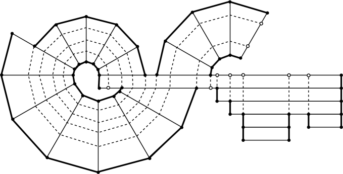
Figure 36. A domain $W$ dissected by isosceles trapezoids and a quadrilateral mesh constructed by propagating non-conforming vertices along $P$-paths (the $P$-sides of the isosceles trapezoids are drawn with a thicker line). However, in general, we need to allow edges that are only “close to parallel” to the base edges. It is proven in [4], that if we allow $\theta$ deviation from parallel, then we can always mesh with $O(n^{2}/\theta^{2})$ quadrilaterals that are $2\theta$-nice.

A chain in a dissection is a maximal collection of distinct trapezoids $T_{1},\dots,T_{k}$ so that for $j=1,\dots k-1$, $T_{j}$ and $T_{j+1}$ share a $Q$-side (i.e., the $Q$-sides are identical, not just overlapping; in other words, the chain of trapezoids forms a quad-mesh of their union). If a trapezoid in the dissection does not share a $Q$-side with any other trapezoid, we consider it as a chain of length one. For example, the dissection on the left of Figure 35 consists of a single chain of length 8. The dissection on the right of Figure 35 consists of a three chains of length 5 (each is similar to the others). The dissection in Figure 36 has chains of length 2, 4, 5 and 7 and four chains of length 1. The ends of a chain consists of two segments: the $Q$-side of $T_{1}$ that is not shared with $T_{2}$, and the $Q$-side of $T_{k}$ that is not shared with $T_{k-1}$. The corners of a chain are the endpoints of the ends of the chain. Usually there are four distinct corners, but there may only be two in the case when $T_{1}$ and $T_{k}$ also share a $Q$-side. In this case, the chain forms a closed loop, and we will call this a closed chain. This case is not of much interest to us since no propagation paths will ever occur inside a closed chain.

The precise result that we will use is Lemma 11.1 of [4]:

Theorem 13.1.

Suppose that $W$ is a polygonal domain with an isosceles trapezoid dissection with $n$ pieces. Suppose also that $0^{\circ}\leq\theta\leq 15^{\circ}$ and that every dissection piece is $\theta$-nice. Finally, suppose the number of chains in the dissection is $M$. Then we can remove $O(M/\theta)$ $\theta$-nice quadrilaterals of uniformly bounded eccentricity from $W$ so that the remaining region $W^{\prime}$ has a $2\theta$-nice quadrilateral mesh with $O(nM/\theta)$ elements. At most $O(M/\theta)$ new vertices are created on the $Q$-boundary of $W^{\prime}$. At most $O(M)$ vertices are created on the $P$-boundary of $W^{\prime}$, and no more than $O(1)$ vertices are placed in any single $P$-side of dissection piece of $W^{\prime}$. For this quad-mesh, any boundary point on a $Q$-side of $W^{\prime}$ propagates to another boundary point after crossing at most $O(n)$ quadrilaterals.

Very briefly, the proof in [4] creates $O(M)$ sub-regions of $W$ called return regions that are chains of isosceles trapezoids with the property that any $P$-path crossing $5n+1$ trapezoids must hit at least one return region. Each return region is sub-divided by $P$-paths into at most $O(1/\theta)$ parallel chains, called tubes, that are each approximately $1/\theta$ times “longer” than they are “wide” (this is made precise in [4]). This property implies that we can place two quadrilaterals inside each tube with the property that any propagation path entering either end of tube can be $\theta$-bent so that it hits a $Q$-side of one of the two quadrilaterals. See Figure 37. This terminates the path. The $O(M/\theta)$ quadrilaterals inside the tubes are the ones that are removed from $W$ to give $W^{\prime}$. There are $O(M/\theta)$ tubes and the corners of these tubes must be $P$-propagated until the hit $\partial W^{\prime}$; this gives the $O(M/\theta)$ boundary vertices that may be created on the $Q$-sides of $W^{\prime}$. The corners of the $O(M/\theta)$ removed quadrilaterals also have to propagated as $Q$-paths, giving points on the $P$-sides of $W^{\prime}$, but by choosing the quadrilaterals appropriately we can arrange for only $O(M)$ vertices to be created on the $P$-sides of $W$, and at most $O(1)$ vertices are added to any single $P$-side of $W^{\prime}$. Since these details of the proof Theorem 13.1 are not needed to apply the result, we refer the reader to [4] for further information.

Figure 37. An example of a return region divided into two tubes and of quadrilaterals placed at opposite ends of these tubes. The corners of these quadrilaterals are connected by a path (dashed) in the tube, dividing it into $2\theta$-nice quadrilaterals. Every path entering the tube will either hit one of the quadrilaterals immediately, or propagate to hit the quadrilateral at the other end of the tube.

14. Thick/thin decompositions and meshing a simple polygon

In this section, we review some facts from [6] about meshing a simple polygon. Most of the discussion is background that motivates the result, but is not needed to apply the result. Theorem 14.1, at the end of the section, will contain the precise statements that we will use.

The papers [5] and [6] make use of a decomposition of a polygon into pieces called the thick and thin parts. The name is motivated by the thick/thin decomposition of a hyperbolic Riemann surface; the $\epsilon$-thin parts of a surface are the points that lie on a closed curve of hyperbolic length $<\epsilon$ that is not deformable to a point (i.e., a homotopically non-trivial loop). A famous theorem of Margulis says that if $S$ is a hyperbolic Riemann surface, then there is an $\epsilon_{0}>0$ (independent of the surface), so that for $\epsilon<\epsilon_{0}$, the $\epsilon$-thin parts are all disjoint. Moreover, each thin part is either a punctured disk (curves around the puncture can be deformed to loops of arbitrarily short length) or a cylinder (there is a positive lower bound for the length of any non-trivial loop in such a thin part). See Figure 38. These two cases are called parabolic and hyperbolic thin parts respectively. The names come from the classification of the group elements that represent these loops when the surface is represented as the hyperbolic unit disk quotiented by a discrete group of Möbius transformations.

Figure 38. A surface with one hyperbolic thin part (darker) and three parabolic thin parts (lighter).

The precise definition of the thin part of a polygon is given in Section 12 of [5]; the construction of the thick and thin parts of a polygon is somewhat involved and makes use of an approximation of the conformal map from the interior of the polygon to the unit disk. For readers who know the terminology, each thin part corresponds to a pair of edges of $P$ whose extremal distance inside $P$ is less than $\epsilon$. Briefly, two sides $e,f$ of a polygon have extremal distance $<\epsilon$ if and only if there is a non-negative function $\rho$ on the interior of $P$ so that:
(1) $\int_{\gamma}\rho ds\geq 1$ for any curve in the interior connecting $e$ to $f$, and
(2) $\iint\rho^{2}dxdy<\epsilon$.
Extremal distance is a conformal invariant that plays a fundamental role in modern complex function theory and dynamics; for its basic properties see [1], [9]. We will not need to understand it to use the results from [5] and [6], but we will use the following fact: if $e$ and $f$ are sides of a polygon $P$ that have small extremal distance in $P$, then they can be joined inside $P$ by a curve $\gamma$ whose length is much less than $\min({\rm{diam}}(e),{\rm{diam}}(f))$. The converse need not be true, i.e., a relatively short joining curve does not imply the extremal distance is small. However, two sides of $P$ that touch at a common vertex must have extremal distance zero; thus there will be a thin part associated to every pair of adjacent edges (parabolic thin parts), and possibly other thin parts associated to non-adjacent pairs of edges (hyperbolic thin parts).

A cross-cut of a domain is a Jordan arc in the domain that has both its endpoints on the boundary of the domain. If the domain is bounded by a Jordan curve, a cross-cut $\gamma$ cuts the domain into two pieces that have $\gamma$ as the intersection of their boundaries. The thick/thin decomposition of a polygon is a special partition of its interior by cross-cuts. A parabolic thin part is bounded by two sub-segments of $P$ meeting at vertex $v$ of $P$ and by a single circular cross-cut (a subset of the circle centered at $v$). The diameter of the piece is small compared to the distance from $v$ to the nearest distinct vertex or non-adjacent edge of $P$ (as measured in the internal path metric). See Figure 39.

A hyperbolic thin part is bounded by two segments on non-adjacent sides of $P$ and two disjoint cross-cuts that connect the endpoints of these segments. The segments have the same length, and the internal path distance between them is much smaller than this length. The cross-cuts are either both concentric circular arcs, or each is the union of two circular arcs. See Figure 39. The thick parts are everything else. Thin parts can only share a cross-cut boundary with a thick part (never an another thin part).

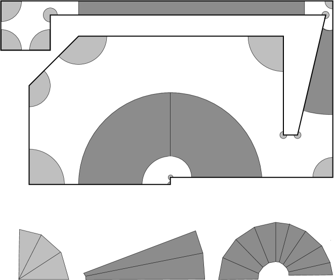
Figure 39. Parabolic thin parts are shown in light gray, hyperbolic thin parts in dark gray and the thick part is the remaining white part of the polygon. It is also possible to inscribe polygonal cross-cuts into these arcs as illustrated on the bottom.

We can replace the circular cross-cuts by inscribing polygonal arcs into these cross-cuts to get polygonal thick and thin parts. This gives thin parts that are simple polygons and it is this type of thin part that we want to use in the proof of Theorem 1.1. In fact, [5] shows that by inscribing $O(1/\theta)$ vertices on each cross-cut, we can ensure that each polygonal hyperbolic thin part is meshed by a chain of $\theta$-nice isosceles trapezoids. However, the eccentricity of these trapezoids may be arbitrarily large, depending on $P$.

In [6] the thick/thin decomposition is applied to quad-meshing as follows. The thin parts come in a small number of very simple shapes and all of these are meshed “by hand”. The thick parts have complex geometry, but the conformal map of a polygon to the unit disk is very well behaved on the thick parts (i.e., there are good estimates of the distortion) and it can be used to transfer nice meshes on the disk (constructed using hyperbolic geometry) back to a nice mesh of the thick part that agrees with the meshes of the thin parts on the common cross-cut boundaries.

The following result includes various facts that are needed in the proof of Theorem 1.1. The result is not stated like this in [6], but all the claims made here are established as part of the proofs in [5] and [6].

Theorem 14.1.

Suppose $P$ is a simple polygon with $n$ vertices. Then $P$ has a decomposition into $O(n)$ simple polygonal pieces of three types: thick pieces, parabolic thin pieces and hyperbolic thin pieces. The total number of edges used in $O(n)$. Suppose $\theta>0$. Then $P$ has a quadrilateral mesh with $O(n/\theta^{2})$ elements that sub-divides the thick/thin decomposition. The mesh quadrilaterals in the thick parts will be called thick quadrilaterals. Similarly for the parabolic quadrilaterals and hyperbolic quadrilaterals. The quad-mesh restricted to each type of piece satisfies the following properties:

Thick pieces: The interior angles of the thick pieces are all either in $[90^{\circ},90^{\circ}+\theta]$ or in $[180^{\circ},180^{\circ}+\theta]$. If a thick piece has $k$ cross-cuts boundary arcs, then the quadrilateral mesh in this piece has $O(k/\theta^{2})$ elements and $O(k/\theta)$ vertices occur on the boundary of the thick piece. The eccentricity of every quadrilateral mesh element in a thick piece is bounded by a constant $M$, independent of anything else. All the mesh elements are nice (angles between $60^{\circ}$ and $120^{\circ}$). Each quadrilateral mesh element in a thick piece has at most one of its sides on $P$.

Parabolic thin pieces: A parabolic thin piece contains exactly one vertex $v$ of $P$. It is bounded by two sub-segments of $P$ and one polygonal cross-cut with $O(1/\theta)$ elements. The mesh in this piece has $O(\theta^{-2})$ elements and $O(\theta^{-1})$ vertices on the boundary of the thin piece. Every angle of the mesh, except possibly one, has angle measure in $[60^{\circ},120^{\circ}]$. The possible exception occurs if the vertex $v$ has interior angle $\alpha<60^{\circ}$ in $P$. In that case, exactly one quadrilateral $Q$ in the mesh of the thin part has $v$ as a vertex and the angle of $Q$ at $v$ is $\alpha$. This quadrilateral is a kite with eccentricity $O(1/\alpha)$; all other quadrilaterals in the mesh of the parabolic thin piece have eccentricity that is uniformly bounded. Each parabolic quadrilateral $Q$ that does not contain a vertex $v$ of $P$ has at most one of its sides on $P$. If $P$ has angle $\leq 120^{\circ}$ at $v$ then the quadrilateral $Q$ having $v$ as a vertex has two sides on $P$. If the angle of $P$ at $v$ is greater than $120^{\circ}$ then the angle is subdivided and there are two or more quadrilateral mesh elements that have $v$ for a vertex, and these all have at most one side on $P$.

Hyperbolic thin pieces: Each hyperbolic thin part is bounded by two sub-segments $S_{1},S_{2}$ of non-adjacent sides of $P$. The endpoints of $S_{1},S_{2}$ are connected by two polygonal cross-cuts with $O(1/\theta)$ edges each. The mesh of the thin part is a chain of $O(1/\theta)$ isosceles trapezoids. The ends of the chain are the segments $S_{1},S_{2}$. Each $P$-side of each trapezoid is also the side of a thick quadrilateral mesh element.

15. The proof of Theorem 1.1

We can now give the proof of Theorem 1.1. We will actually prove the following result that implies Theorem 1.1 if we set $\theta=15^{\circ}$ (the proof simplifies slightly in this case and the reader may wish to first read it with this in mind):

Theorem 15.1.

Suppose $\Gamma$ is a PSLG with $n$ vertices and suppose $0<\theta<90^{\circ}$. Then there is a nice conforming quadrilateral mesh of $\Gamma$ such that

1. every angle of every quadrilateral is $\leq 120^{\circ}$,

2. every new mesh angle is $\geq 60^{\circ}$, i.e., all angles are $\geq 60^{\circ}$ unless the angle occurs at a mesh vertex that is a vertex of $\Gamma$ and the edges of the corresponding quadrilateral lie on edges of $\Gamma$ that make an angle $\alpha<60^{\circ}$ with each other. In this case, the angle of the mesh element there is also $\alpha$ (small angles of the PSLG are not sub-divided),

3. the mesh uses $O(n^{2}/\theta^{2})$ quadrilaterals,

4. all the mesh angles actually lie in the smaller interval from $90^{\circ}-2\theta$ to $90^{\circ}+2\theta$ with at most $O(n/\theta^{2})$ exceptions.

Taking $\theta$ small, we see that in the worst case there are quadratically many mesh elements, but they are all close to rectangles with only a linear number of exceptions. Taking $\theta=15^{\circ}$ we see that a PSLG with $n$ vertices has a conforming mesh with $O(n^{2})$ elements that are all nice with at most $O(n)$ exceptions (one for each interior angle of measure less than $60^{\circ}$ of some face of $\Gamma$.

Proof of Theorem 15.1.

We give the construction of the mesh as a series of steps, and then we will count the number of mesh elements created.

Step 1: Using Lemma 3.1 we reduce to the case when $\Gamma$ is already meshed by $O(n)$ simple polygons and has $O(n)$ vertices and edges.

Step 2: For each vertex $v$ of $\Gamma$, we choose a disk $D$ centered at $v$ with diameter much smaller than the distance to the nearest distinct vertex or edge of $\Gamma$. Inside $D\cap{\rm{PH}}(\Gamma)$ we place a $5^{\circ}$-conforming sink using Lemma 5.3. The interiors of these conforming sinks are called the protected regions. The only quadrilaterals in our final mesh that will have angles less than $60^{\circ}$ are those at the center these protecting sinks, and only when there are edges of $\Gamma$ that touch $v$ making angle $<60^{\circ}$. These quadrilaterals touching $v$ will not be altered by any later step of the construction.

Note that when we define the boundary of the protecting sink for $D$, we can assume that each connected component of $\partial D\setminus\Gamma$ is divided into equal sized intervals by the boundary vertices of the sink (when a component has angle measure less than $5^{\circ}$ it contains a single boundary edge of the sink; otherwise the boundary of the sink inscribed on this arc consists of subarcs of equal angle measure $\leq 5^{\circ}$). This fact will be used later to show that protecting sinks do not touch hyperbolic thin parts in the unprotected region.

Step 3: Note that the unprotected region is now meshed by simple polygons where all the angles are either close to $90^{\circ}$ or close to $180^{\circ}$. The former occurs where boundaries of the protecting sinks meet the edges of $\Gamma$, and the latter occur at other boundary vertices of the protecting sinks. More precisely, the non-protected region of ${\rm{PH}}(\Gamma)$ is now meshed by simple polygons $\{P_{j}\}$ with all angles either in $[90^{\circ},95^{\circ}]$ or $[180^{\circ},185^{\circ}]$. By Theorem 14.1 each such face in the unprotected region can be nicely meshed using $O(k/\theta^{2})$ quadrilaterals having the properties listed in Theorem 14.1, where $k$ is the number of sides of that face. Summing over all the simple polygons shows that $O(n/\theta^{2})$ quadrilaterals are used overall.

Step 4: By Theorem 14.1, the thick quadrilaterals have uniformly bounded eccentricity independent of the polygon. Each such quadrilateral can share at most one side with $P$. We place a sink in each thick quadrilateral.

Step 5: Similarly, the parabolic quadrilaterals have bounded eccentricity if the angles of the polygon are bounded away from zero, which occurs in our case (as noted in Step 3, we only apply the thick/thin decomposition to a polygon where all the angles are $\geq 90^{\circ}$). Thus all the parabolic quadrilaterals have uniformly bounded eccentricities. We place a sink in every parabolic quadrilateral.

Step 6: By Theorem 14.1, the hyperbolic quadrilaterals are all $\theta$-nice isosceles trapezoids and each hyperbolic thin part consists of a chain of such trapezoids. The $P$-sides of these trapezoids agree with sides of thick quadrilaterals and their $Q$-sides either agree with the $Q$-sides of other elements of the chain or they lie on $P$. Thus the union $W$ of all the closed hyperbolic quadrilaterals has a dissection by $\theta$-nice, isosceles trapezoids that has $N=O(n/\theta)$ elements but only $M=O(n)$ chains. Theorem 13.1 says that we can remove $O(M)=O(n)$ nice quadrilaterals with uniformly bounded eccentricity from $W$ to obtain a region $W^{\prime}$, such that $W^{\prime}$ can be $2\theta$-nicely meshed using $O(MN/\theta)=O(n^{2}/\theta^{2})$ quadrilaterals. The mesh creates at most $O(n/\theta)$ new vertices on the $Q$-sides $\partial W^{\prime}$ and at most $O(1)$ vertices on each $P$-side of $W^{\prime}$.

Step 7: Place sinks in each of the nice quadrilaterals in $W\setminus W^{\prime}$ (i.e., the quadrilaterals removed from $W$). Any extra vertices coming from propagation through the mesh of $W^{\prime}$ always land on a single pair of opposite sides of such a quadrilaterals (the $Q$-sides), and so the removed quadrilaterals can be remeshed using a number of elements that is comparable to the number of extra vertices.

Step 8: On the boundary of $W^{\prime}$ there may be points that correspond to vertices of adjacent sinks, but are not vertices of the mesh of $W^{\prime}$. Propagate such points through the mesh of $W^{\prime}$ until they connect with another boundary point of $W^{\prime}$. There are at most $O(n/\theta)$ such boundary points ($O(1)$ for each sink) and each propagation path has length $O(N)=O(n/\theta)$ by Theorem 13.1. Thus at most $O(n^{2}/\theta^{2})$ new mesh elements are created.

Step 9: Next we use the re-meshing property of sinks. To make sure every sink has an even number of points on its boundary, we first bisect the mesh on $W^{\prime}$ (i.e., split every quadrilateral into four by bisecting all four edges) and then we split every boundary edge of every sink into two equal sub-edges. This includes both the sinks placed in thick quadrilaterals (Step 4) and thin parabolic quadrilaterals (Step 5), as well as the protecting sinks placed around each original vertex (Step 2). This doubles the number of vertices on the boundary of each sink, and hence this number is even for each sink. Re-mesh the interiors of all the sinks to conform with these vertices. The meshes on the sinks and on $W^{\prime}$ now match each other along all common edges so we have the desired conforming mesh of $\Gamma$.

This completes the construction of the mesh.

Finally, we have to count the total number of mesh elements that we have created. We are interested both in the total number of elements and in the number of elements that are not $2\theta$-nice. From our remarks above, the number of mesh elements inside $W^{\prime}$ is $O(n^{2}/\theta^{2})$ and all of these are $2\theta$-nice. (The original mesh of $W^{\prime}$ is $2\theta$-nice by Theorem 13.1; any further quadrilaterals in $W^{\prime}$ are formed by standard propagation paths, and these preserve niceness by Lemma 4.2.)

Next we consider elements created when remeshing the sinks. Each sink has some share of the $O(n/\theta)$ vertices that are created on the boundary of $W^{\prime}$. It also has $O(1)$ other extra vertices that come from adjacent sinks. There are four types of sinks that have to be considered:

Protecting sinks: We claimed earlier that at most $O(d)$ points would be added to boundary of a sink protecting a vertex of degree $d$. To prove this claim we will show that the boundary of a protecting sink can only touch thick or parabolic quadrilaterals, never a hyperbolic quadrilateral, and hence the protecting sinks never touch $W^{\prime}$. More precisely,

Lemma 15.2.

An edge $e$ of the boundary of a sink protecting a vertex $v$ of $\Gamma$ never touches a hyperbolic thin part in the unprotected region.

Proof.

Suppose $e$ is a boundary edge of a protecting sink that also lies on the boundary of a face $P$ of the unprotected region, and suppose that $e$ contains the side of a hyperbolic thin part in $P$. Then $e$ would have to have small extremal distance in $P$ to some other side $f$ of $P$. By the definition of hyperbolic thin parts, $e$ and $f$ cannot be adjacent on $P$, and by properties of extremal distance, the path distance between $e$ and $f$ inside $P$ would have to be much smaller than the diameter of either $e$ or $f$. The disk $D$ containing the sink was chosen to be small compared to the distance of $v$ to other vertices and edges of $\Gamma$, and hence all edges of $P$ that do not touch the boundary of the sink have a distance from the sink that is much larger than the diameter of the sink itself. Hence $f$ must lie on one of the edges of $\Gamma$ that define the sector containing $e$, or $f$ must be another boundary edge of the same sink (and inside the same sector as $e$). However, both these alternatives are impossible. By the way that the protecting sinks are constructed in Step 2, each boundary edge of the sink in the sector has the same length. If $f$ is a subsegment of $\Gamma$, then $e$ is not adjacent to $f$ and hence it must be separated from $f$ by a distance comparable to its own diameter. On the other hand, if $f$ is on the boundary of the sink, then $e$ and $f$ have the same diameter and since they are not adjacent, they must be separated by a third edge of the same size. Hence there is no side $f$ of $P$ with small extremal distance to $e$, and the lemma is proven. ∎

Thus the only extra vertices that are added to the boundaries of protecting sinks are due to sink vertices corresponding to adjacent thick or parabolic quadrilaterals. The number of such points is $O(1)$ per quadrilateral and there are at most $O(d)$ such quadrilaterals, so by Lemma 5.3 the total number of mesh elements used in a protecting sink is $O(d^{2})$ where $d$ is the degree of the vertex being protected. Also by Lemma 5.3, at most $O(d/\theta)$ of the mesh elements are not $\theta$-nice. Since summing $d$ over all protecting sinks gives at most $O(n)$, see that at most $O(n^{2})$ mesh elements are used inside protecting sinks, and that at most $O(n/\theta)$ of these are not $2\theta$-nice.

Thick quadrilateral sinks: there are $O(n/\theta^{2})$ such quadrilaterals and hence $O(n/\theta^{2})$ elements in the corresponding sinks (because of uniformly bounded eccentricity). Each thick quadrilateral shares at most one edge with $P$. Hence each thick quadrilateral can share at most one edge with a $Q$-side of $W^{\prime}$ and may share a second side with $P$-side of $W^{\prime}$ (this would be a $P$-side of a hyperbolic quadrilateral in $P$). Thus there is at most one side of the thick quadrilateral that gets more than $O(1)$ extra boundary vertices. Thus if $K$ extra vertices are added from $W^{\prime}$, the re-meshing can be done with $O(K)$ extra elements. Summing over all thick quadrilaterals gives $O(n/\theta)$ extra mesh elements, so the total is still $O(n/\theta^{2})$

Thin quadrilateral sinks: A thin quadrilateral $Q$ can share either zero, one or two sides with the simple polygon $P$ that contains it. In the first two cases, $Q$ can share at most one side with $W^{\prime}$ and the other sides each have at most $O(1)$ extra vertices, due to sinks in adjacent quadrilaterals. Moreover, there are $O(n/\theta^{2})$ such quadrilaterals and there are $O(n/\theta)$ vertices on the boundary of $W^{\prime}$. Thus summing the number of elements in the remeshings of all such quadrilaterals gives at most $O(n/\theta^{2})$ mesh elements in total. All could be non-$\theta$-nice.

If $Q$ shares two sides with $P$, we claim that at most one of these sides is on $\partial W^{\prime}$. To see this, note if $Q$ has two sides on $P$, then $Q$ contains a vertex $v$ of $P$. If the angle of $P$ at $v$ close to $180^{\circ}$, then the method from [6] subdivides the angle at $v$ and any quadrilaterals containing $v$ have at most one edge with $P$. Thus the angle of $P$ at $v$ must be close to $90^{\circ}$. However, this implies $Q$ has one side on the boundary of a protecting sink, and hence at most one side can be on $\partial W^{\prime}$.

Thus the analysis in this case (2 sides on $P$) is the same as in the two previous cases (0 or 1 side on $P$). Actually, it is a little better since there are only $O(n)$ such parabolic quadrilaterals instead of $O(n/\theta^{2})$ as in the previous two cases.

Quadrilateral sinks removed from $W$: these all have uniformly bounded eccentricity and extra vertices coming from propagation through $W^{\prime}$ are only added to a single pair of opposite sides (the $Q$-sides). Thus if $K$ vertices are added to such a sink, the re-meshing can be accomplished with $O(K)$ elements. There are $O(n/\theta)$ propagation paths that can add extra vertices, so summing over all such quadrilaterals, gives $O(n/\theta)$ mesh elements inside the removed quadrilaterals.

In conclusion, the total number of mesh elements is $O(n^{2}/\theta^{2})$ (the dominant terms are $O(n/\theta^{2})$ from the mesh of $W^{\prime}$ and $O(n^{2})$ from the protecting sinks). The number of mesh elements that are not $2\theta$-nice is $O(n/\theta^{2})$ (this includes all the mesh elements in the last four categories of sinks above, plus the number of non-$\theta$-nice mesh elements that can occur in protecting sinks). This completes the proof of Theorem 15.1, and hence of Theorem 1.1 as well. ∎

Taking a fixed $\theta$, say $\theta=15^{\circ}$, the mesh of $\Gamma$ has only $O(n)$ vertices on the boundary of the polynomial hull of $\Gamma$ and all but $O(n)$ of the interior vertices have all angles close to $90^{\circ}$, so

Corollary 15.3.

The mesh in Theorem 1.1 can be taken so that all but $O(n)$ vertices have degree four.

This implies that the mesh can be partitioned into $O(n)$ (combinatorial) rectangular grids using motorcycle graphs as described by Eppstein, Goodrich, Kim and Tamstorf in [8]. Hence the mesh is completely described by a graph of size $O(n)$ with integer labels on the edges; the vertices of the graph are the corners of the rectangular pieces, edges of the graph correspond to a shared boundary arc of two rectangular pieces, and the labels give the number of mesh elements on this shared boundary arc (e.g., see Figure 5 of [8]). Thus, although the mesh in Theorem 1.1 may have $O(n^{2})$ elements, it only has complexity $O(n)$ in a certain sense. Can this observation be exploited in numerical methods that make use of quadrilateral meshes?

References

- [1] L. V. Ahlfors. Lectures on quasiconformal mappings. The Wadsworth & Brooks/Cole Mathematics Series. Wadsworth & Brooks/Cole Advanced Books & Software, Monterey, CA, 1987. With the assistance of Clifford J. Earle, Jr., Reprint of the 1966 original.
- [2] M. Bern and D. Eppstein. Quadrilateral meshing by circle packing. Internat. J. Comput. Geom. Appl., 10(4):347–360, 2000. Selected papers from the Sixth International Meshing Roundtable, Part II (Park City, UT, 1997).
- [3] M. Bern, S. Mitchell, and J. Ruppert. Linear-size nonobtuse triangulation of polygons. Discrete Comput. Geom., 14(4):411–428, 1995. ACM Symposium on Computational Geometry (Stony Brook, NY, 1994).
- [4] C.J. Bishop. Nonobtuse triangulations of PSLGs. to appear, Discrete and Computational Geometry.
- [5] C.J. Bishop. Conformal mapping in linear time. Discrete Comput. Geom., 44(2):330–428, 2010.
- [6] C.J. Bishop. Optimal angle bounds for quadrilateral meshes. Discrete Comput. Geom., 44(2):308–329, 2010.
- [7] D. Eppstein. Faster circle packing with application to nonobtuse triangulation. Internat. J. Comput. Geom. Appl., 7(5):485–491, 1997.
- [8] D. Eppstein, M.T. Goodrich, E. Kim, and R. Tamstorf. Motorcycle graphs: Canonical quad mesh partitioning. Eurographics Symposium on Geometric Processing 2008, 27(5), 2009.
- [9] J.B. Garnett and D.E. Marshall. Harmonic measure, volume 2 of New Mathematical Monographs. Cambridge University Press, Cambridge, 2005.