Structured identification for network reconstruction of RC-models

Abstract

Resistive-capacitive (RC) networks are used to model various processes in engineering, physics or biology. We consider the problem of recovering the network connection structure from measured input-output data. We address this problem as a structured identification one, that is, we assume to have a state-space model of the system (identified with standard techniques, such as subspace methods) and find a coordinate transformation that puts the identified system in a form that reveals the nodes connection structure. We characterize the solution set, that is, the set of all possible RC-networks that can be associated to the input-output data. We present a possible solution algorithm and show some computational experiments.

Keywords: Structured identification, RC-networks, algebraic methods.

1 Introduction

Various dynamical models of processes in engineering, physics or biology have the following form

$$\begin{array}[]{ll}G\dot{x}(t)=Sx(t)+Bu(t)\\ y(t)=Cx(t)\,,\end{array}$$ (1)

where $x(t)\in\mathbb{R}^{n}$ is the state, $u(t)\in\mathbb{R}^{m}$ is the input, $y(t)\in\mathbb{R}^{p}$ is the output. We assume that $S\in\mathbb{R}^{n\times n}$ is symmetric, $G\in\mathbb{R}^{n\times n}$ is diagonal and positive definite, while $B$ and $C$ have no special structure.

For instance, model (1) may represent a generic RC (resistive and capacitive) network, in which the components of $x\in\mathbb{R}^{n}$ are the node potentials, $S$ is the admittance matrix and the diagonal elements of $G$ are the nodes capacitances. As an example, consider the RC circuit represented in Figure 3 and assume that the output is the potential of node $A$. The corresponding model has form (1):

$$\begin{gathered}\left(\begin{array}[]{cc}C_{1}&0\\ 0&C_{2}\end{array}\right)\left(\begin{array}[]{cc}\dot{v}_{1}(t)\\ \dot{v}_{2}(t)\end{array}\right)\\ =\left(\begin{array}[]{cc}-R_{1}^{-1}-R_{12}^{-1}&R_{12}^{-1}\\ R_{12}^{-1}&-R_{2}^{-1}-R_{12}^{-1}\end{array}\right)\left(\begin{array}[]{cc}v_{1}(t)\\ v_{2}(t)\end{array}\right)\,,\end{gathered}$$ (2)

$$y(t)=\left(\begin{array}[]{cc}1&0\end{array}\right)\left(\begin{array}[]{cc}v_{1}(t)\\ v_{2}(t)\end{array}\right)\,.$$

We can associate a weighted undirected graph to matrix $S$ in (1) by considering $S$ a weighted adjacency matrix. Namely, we define a node for each component of vector $x$ and we define an edge between node $i$ and node $j$ if the entry of row $i$ and column $j$ of $S$ is nonzero. The numerical value of the entry represents the edge weight. For instance, Figure 2 represents the graph associated to the model of the circuit in Figure 3.

For simplicity, in the rest of the paper we will omit self loops when representing the graph associated to the $S$ matrix of a system in form (1),

Figure 1: Example of an RC-circuit.

Figure 2: Graph representation of model associated to the circuit in Figure 3.

Form (1) can also be used to model those systems that have the same mathematical representation of RC-circuits, such as thermal systems, physical network systems ([1]), dendritic structures ([2]), mammillary systems ([3]), or, more generally, diagonally symmetrizable compartmental systems (see [4]).

Consider a second system of form

$$\begin{array}[]{ll}\dot{z}(t)=\hat{A}z(t)+\hat{B}u(t)\\ y(t)=\hat{C}z(t)\,,\end{array}$$ (3)

in which $\hat{A}$, $\hat{B}$, $\hat{C}$ have the same dimensions of $S$, $B$, $C$. In this paper we consider the following algebraic problem.

Problem 1.

Consider systems (1), (3), where matrices $\hat{A},\hat{B},\hat{C},B,C$ are given. Find, if possible, an invertible matrix $T$, a symmetric matrix $S$ and a strictly positive diagonal matrix $G$ such that

$$\left\{\begin{array}[]{ll}T^{-1}\hat{A}T=G^{-1}S\\ \hat{C}T=C\\ T^{-1}\hat{B}=G^{-1}B\,.\end{array}\right.$$ (4)

In other words, we are looking for a state-space transformation of form $z=Tx$ and suitable matrices $S$ and $G$ such that (3) takes on form (1).

Problem 1 can be interpreted as a structured identification one. Namely, system (3) represents an identified black-box model, obtained from experimental data with standard techniques, for instance state space identification methods. Our aim is to check if this system, after state transformation $z=Tx$, can be given the form of model (1), and, if this is possible, find such a transformation. The structural requirements imposed in Problem 1 are the following ones

• The transformed system matrix $T^{-1}\hat{A}T$ must be the product of a positive diagonal and a symmetric matrix.

• The input and output matrices are assigned.

The first requirement ensures that the transformed system matrix can be written as the product of a diagonal matrix (containing the inverse capacities, in the case of RC-circuits) and a symmetric matrix (the admittance matrix in the case of RC-circuits). The second requirement is due to the fact that, in some cases, the input matrix $B$ or the output matrix $C$ may be known from structural properties of the system at hand. For instance, in an RC-circuit we may be able to measure the potential of the first $n_{1}$ nodes, while the potentials of the remaining ones are not accessible. In this case, $C$ would correspond to the projection matrix on the first $n_{1}$ components. Note that we may not have this requirement on $B$ or $C$. In this case, the second, the third condition in (4), or both could be omitted.

Further, we consider a more restrictive version of Problem 1, based on the observation that, in various dynamical models, matrix $S$ in (1) is Metzler, that is, all its off-diagonal entries are non-negative. For instance, in RC-networks, off-diagonal entries correspond to the values of the resistances connecting the network nodes (see (2)). This suggests the following formulation.

Problem 2.

Solve Problem 1 with the additional requirement that $S$ is Metzler.

Further, if Problem 2 has multiple solutions, one may minimize the number of nonzero components of $S$, that is, minimize $\|S\|_{0}$, the so-called zero-norm of $S$. This follows the principle of parsimony of finding the simplest model of form 1 that fits the data. This leads to the following additional problem.

Problem 3.

Find the solutions of Problem 2 in which $\|S\|_{0}$ is minimum.

For instance, in an RC-circuit, the nonzero elements of $S$ represent the resistive connections between the nodes. Hence, minimizing $\|S\|_{0}$ corresponds to reducing the overall number of resistive components.

1.1 Statement of contribution

Regarding Problem 1, we will show that it is convenient to parameterize the set of solutions as $T=PQ\sqrt{G}$, where $P$, $Q$ is the polar decomposition of $T\sqrt{G}^{-1}$. In particular,

• Proposition 4 shows that $P$ and $G$ are the solution of a problem with a reduced number of unknowns. Essentially, this result leverages the symmetry of $S$. Further, if either the second or the third condition in (4) is missing, $P$ and $G$ are the solution of a convex problem. We will consider this last case in more detail. We will mention that, in many cases, the solution $P$, $G$ is unique up to a scaling factor.

• Proposition 7 parameterizes all solutions of $Q$ corresponding to each solution $P$, $G$.

These results can also be used to reduce the number of unknowns in Problems 2 and 3. Anyway, these last two problems are more difficult than Problem 1. To solve them, we will resort to general local search algorithms.

1.2 Comparison with literature

A problem similar in structure to Problem 1, but more general, consists in solving the following system with respect to unknown parameter vector $\theta$

$$\left\{\begin{array}[]{ll}T^{-1}\hat{A}T=A(\theta)\\ \hat{C}T=C(\theta)\\ T^{-1}\hat{B}=B(\theta)\,,\end{array}\right.$$ (5)

in which matrices $A$, $B$, $C$ depend on $\theta$. Problem 1 may be considered a special case of (5), in which $C$ and $B$ do not depend on $\theta$ and the only constraint on $A$ is symmetry.

Problem (5) has been extensively studied in recent literature. A common approach consists in two phases. First, one finds a black-box model (this is in general an easy one, for instance, resorting to subspace-based methods). Second, one finds a coordinate transformation $T$ and a parameter vector $\theta$ that satisfy (5). In the general case, this second step is not an easy task. In fact, even assuming, as commonly done, that $A$, $B$, $C$ are a linear function of $\theta$, Problem (5) is bilinear and, thus, nonconvex.

This approach has been introduced in [5] and studied in various subsequent works. For instance, [6] studied the problem of parameter initialization. Works [7], [8], [9], [10] present different numerical approaches for the solution.

With respect to these general approaches, this work leverages the special structure imposed by Problem (1), in particular the symmetry of $S$ to obtain specific properties (see Propositions 4 and 7) that do not apply to the more general case (5). As far as we know, the results presented in these two propositions are new, perhaps also due to the specificity of the problem discussed in this paper.

In literature, we can also find approaches for network topology reconstruction not based on structured identification, such as [11, 12, 13].

Notation: Matrix $A\in\mathbb{R}^{n\times n}$ is diagonalizable if there exist a nonsingular matrix $V$ and a diagonal matrix $\Lambda$ such that $AV=V\Lambda$. The columns of $V$ are the right eigenvectors of $A$. Set $W=V^{-1}$, then we have that $WA=V^{-1}A=\Lambda V^{-1}=\Lambda W$, which shows that the rows of $W$ are left eigenvectors of $A$. We also write that $(V,\Lambda,W)$ is a diagonalization of $A$. We denote the orthogonal group over $\mathbb{R}$ by

$$\begin{array}[]{ll}O(n)=\{M\in\mathbb{R}^{n\times n}\textrm{ such that }M\textrm{ is invertible}\textrm{ and }M^{T}M=I\},\end{array}$$

that is the set of real orthonormal matrices of dimension $n$. Given a subspace $V\subset\mathbb{R}^{n}$, we will denote by $V^{\perp}$ its orthogonal subspace.

2 Discussion of Problem 1

The following proposition presents a necessary condition for the feasibility of Problem 1.

Proposition 1.

Problem 1 has a solution only if $\hat{A}$ is diagonalizable and has real eigenvalues.

Proof.

Assume that Problem 1 has a solution. By the first of (4) it follows that $G^{1/2}T^{-1}\hat{A}TG^{-1/2}=G^{-1/2}SG^{-1/2}$. Note that this last matrix is symmetric, hence $\hat{A}$ is diagonalizable and has real eigenvalues, being similar to a symmetric matrix. ∎

Due to the previous proposition, we will make this assumption throughout the paper.

Assumption 1.

$\hat{A}$ is diagonalizable and has real eigenvalues

Remark 1.

By Proposition 1, if Assumption 1 does not hold for $\hat{A}$, then Problem 1 does not have a solution. This means that the identified system has not the structure of an RC-network.

We will parameterize the set of possible solutions $T$ of Problem 1 as

$$T=PQ\sqrt{G}\,,$$ (6)

where $P$ is a symmetric and positive definite matrix and $Q\in O(n)$. Note that $PQ$ corresponds to the left polar decomposition of $T\sqrt{G}^{-1}$, which is unique, being $T\sqrt{G}^{-1}$ invertible. In particular, $P$ corresponds to a scaling and $Q$ to a rotation or reflection, further $P=\sqrt{TG^{-1}T^{T}}$. In the following, we will show that parameterization (6) is convenient since couple $P$, $G$ can be found separately from $Q$. As a first step, the following proposition shows that the feasibility of Problem 1 is equivalent to the existence of a solution of an equation independent of $Q$. The proof is presented in the Appendix.

Proposition 2.

Problem 1 has a solution $T,S,G$ if and only if there exists a positive definite matrix $M$ such that

$$\left\{\begin{array}[]{lll}\hat{A}M=M\hat{A}^{T}\\ \hat{C}M\hat{C}^{T}=CG^{-1}C^{T}\\ \hat{B}^{T}M^{-1}\hat{B}=B^{T}G^{-1}B\\ \hat{C}\hat{B}=CG^{-1}B.\end{array}\right.$$ (7)

Moreover, $M=P^{2}$, where $P$ is defined as in (6) .

Note that, with respect to form (6), equation (7) contains variables $M=P^{2}$, $G$, but does not contain $Q$. The structure of (7) can be simplified by diagonalizing $\hat{A}$. It particular, if $(V,\Lambda,W)$ is a diagonalization of $\hat{A}$ (i.e., $\hat{A}=V\Lambda W$), the following proposition shows that the first equation in (7) can be substituted with $M=VDV^{T}$, where $D$ is a matrix that commutes with $\Lambda$ (i.e., $D\Lambda=\Lambda D$).

Proposition 3.

Let $(V,\Lambda,W)$ be a diagonalization of $\hat{A}$ and let $M\in\mathbb{R}^{n\times n}$, then the following statements are equivalent

i) $\hat{A}M=M\hat{A}^{T}$

ii) there exists a matrix $D$, that commutes with $\Lambda$, such that $M=VDV^{T}$.

Proof.

i) $\Rightarrow$ ii) Substituting $\hat{A}=V\Lambda V^{-1}$ in i) we obtain $V\Lambda V^{-1}M=MV^{-T}\Lambda V^{T}$, which implies $\Lambda V^{-1}MV^{-T}=V^{-1}MV^{-T}\Lambda$. Set $D=V^{-1}MV^{-T}$, then $\Lambda D=D\Lambda$ and $M=VDV^{T}$.

ii) $\Rightarrow$ i) Let $D$ be any matrix such that $\Lambda D=D\Lambda$ and set $M=VDV^{T}$. Then $\hat{A}M=\hat{A}VDV^{T}=V\Lambda V^{-1}VDV^{T}=V\Lambda DV^{T}=VD\Lambda V^{T}=VDV^{T}V^{-T}\Lambda V^{T}=M\hat{A}^{T}$.

∎

Remark 2.

The requirement that $D$ commutes with $\Lambda$ limits the actual number of unknown entries of $D$. In fact, setting $\Lambda=\textrm{diag }\{\lambda_{1},\ldots,\lambda_{n}\}$, $D=(d_{ij})$ commutes with $\Lambda$ if and only if

$$d_{ij}=0,\textrm{ for all }i,j\textrm{ such that }\lambda_{i}\neq\lambda_{j}\,.$$

For instance, if all eigenvalues of $A$ are distinct, $D$ must be diagonal. In the general case, $D$ has a block-diagonal structure.

Combining the results of Propositions 2 and 3, we derive the following result.

Proposition 4.

Problem 1 has a solution $T,S,G$ if and only if there exist a symmetric matrix $D$ and a diagonal matrix $G$ such that

$$\left\{\begin{array}[]{lll}D>0\\ \Lambda D=D\Lambda\\ G>0\\ \hat{C}VDV^{T}\hat{C}^{T}=CG^{-1}C^{T}\\ \hat{B}^{T}W^{T}D^{-1}W\hat{B}=B^{T}G^{-1}B\\ \hat{C}\hat{B}=CG^{-1}B.\end{array}\right.$$ (8)

Moreover, $P=\sqrt{VDV^{T}}$, where $P$ is defined in (6).

In Problem (8) the optimization variables are $D$ and $G$. This problem is nonconvex, since variable $D$ appears in it together with its inverse.

Remark 3.

If the third condition is not present in (4), the third and fourth conditions disappear from (7) and, setting $H=G^{-1}$, problem (8) reduces to a convex one:

$$\left\{\begin{array}[]{lll}D>0\\ \Lambda D=D\Lambda\\ H>0\\ \hat{C}VDV^{T}\hat{C}^{T}=CHC^{T}\,.\end{array}\right.$$ (9)

The fact that the third condition is not present in (4) means that we do not impose any structural requirement on matrix $B$. The solution of (9) is not unique. In fact, if $D$, $H$ is a solution of (8), any scaling $\alpha D$, $\alpha H$, with $\alpha>0$ is still a solution.

In particular, if $\hat{A}$ has distinct eigenvalues, $D$ must be diagonal and Problem (9) reduces to finding positive diagonal matrices $D$, $H$ such that

$$\hat{C}VDV^{T}\hat{C}^{T}=CHC^{T}.$$ (10)

The set of all solutions of (9) corresponds to a polyhedral cone and can be expressed as a conical combination of a finite set of vertices (by Weyl-Minkowski theorem), that is, we can find vectors $v_{1},\ldots,v_{l}$ (called generators) such that the set of all solutions of (9) is

$$\{\alpha_{1}v_{1}+\alpha_{2}v_{2}+\ldots+\alpha_{l}v_{l},\quad\alpha_{1},\alpha_{2},\ldots,\alpha_{l}>0\}.$$ (11)

These considerations also hold if the second condition of (4) is not present.

Remark 4.

We present an intuitive discussion on the number of distinct solutions of (9). Assuming $\hat{A}$ has distinct eigenvalues, so that $D$ is diagonal, Problem (9) reduces to finding positive diagonal matrices $D$, $H$ such that (10) holds. The solutions of (10) are represented by vector $x=[\textrm{diag }{D},\textrm{diag }{H}]$, that contains the elements on the diagonal of the two matrices $D$ and $H$.

Note that, since the left and right-hand sides of this expression are symmetric $p\times p$ matrices, this corresponds to a set of $n_{e}=\frac{p(p+1)}{2}$ equations. We have $n_{u}=2n$ unknown terms (the diagonal elements of $D$ and $H$). Hence, for a generic choice of problem data (i.e., matrices $\hat{A}$, $C$, $\hat{C}$ are randomly selected) we have a solution consisting of a unique ray (that is, unique up to scaling) if $n_{e}\geq n_{u}-1$, that is $p\geq\frac{\sqrt{16n-7}-1}{2}$, where the $-1$ term is due to the fact that a ray has dimension one. However, if the problem data are not generic, we may have multiple solutions even if this condition is satisfied. For instance, if $C$ is a projection on the first $p$ components, then term $CHC^{T}$ does not contain the last $n-p$ elements of the diagonal of $H$. Hence, these are left undetermined and can be chosen as arbitrary positive values. In this case, the number of remaining unknowns is $n_{u}=n+p$, so that, if remaining parameters $\hat{A}$, $\hat{C}$ are generic, we have only one solution for $D$ and for the first $p$ elements of the diagonal of $H$ (up to a scaling factor) if $n_{e}\geq n_{u}-1$, that is

$$p\geq\frac{\sqrt{8n-7}+1}{2}\,.$$ (12)

These considerations intuitively justify the fact that, in generic cases, if $p$ is sufficiently high, equation (9) has only one solution (up to a scaling factor). Our numerical experiments confirm this fact, however, we do not have a formal proof.

Example 1.

Consider the RC circuit depicted in Figure 3.

Figure 3: Circuit used in Example 1.

If $x(t)\in\mathbb{R}^{4\times 1}$ represents the node potentials, $C_{1}=C_{2}=C_{3}=C_{4}=1$, $R_{1}=R_{4}=R_{2}=1$, $R_{3}=2$, the model of the system corresponds to (1) with $G=I$ and

$$S=\left(\begin{array}[]{cccc}-4&1&1&2\\ 1&-1&0&0\\ 1&0&-2&1\\ 2&0&1&-3\end{array}\right).$$ (13)

We assume that the system is autonomous (i.e., $B$ is not present) and the outputs are the potentials of the first three nodes, that is

$$C=\left(\begin{array}[]{cccc}1&0&0&0\\ 0&1&0&0\\ 0&0&1&0\end{array}\right).$$

Suppose that we do not known matrices $G$ and $S$, but we do know matrix $C$, since our output consists in the potentials of the first three nodes. Assume also that, by using standard identification techniques (for instance subspace-based methods), we are able to identify a state-space model in form

$$\begin{array}[]{ll}\dot{z}(t)=\hat{A}z(t)\\ y(t)=\hat{C}z(t)\,,\end{array}$$

with

$$\hat{A}=\left(\begin{array}[]{cccc}-10&-4&-23&5\\ 1&-1&3&-1\\ 3&1&7&-2\\ 1&-1&3&-4\end{array}\right),\hat{C}=\left(\begin{array}[]{cccc}1&0&3&-1\\ 0&1&0&0\\ 0&-1&1&0\end{array}\right).$$

Then, solving Problem 1 consists in finding a coordinate transformation $x=Tz$ and matrices $G$ and $S$ such that (4) holds. In particular, matrix $S$ is a key piece of information since it allows to reconstruct the network structure. Note that assumption 1 is satisfied. We use parameterization (6) and apply Proposition 4 to find matrices $P$ and $G$. Since we do not have any requirement on input matrix $B$, we have to solve convex problem (9). Further, since $\hat{A}$ has distinct eigenvalues, by Remark 2, $D$ must be diagonal, so that Problem (9) reduces to the following linear one, in which the variables are the diagonal matrices $D$ and $H$,

$$\left\{\begin{array}[]{lll}D>0\\ H>0\\ \hat{C}VDV^{T}\hat{C}^{T}=CHC^{T}\,.\end{array}\right.$$ (14)

As previously noted, the solution to this problem is not unique, since, if $D$ and $H$ are a solution of (14) for any $\alpha\in\mathbb{R}$, with $\alpha>0$, also $\alpha D,\alpha H$ is a solution of (14). The solution set has form (11), in particular there are two generators, so that the set of all solutions is given by

$$x=\{v_{1}\alpha_{1},v_{2}\alpha_{2}\},$$ (15)

with $v_{1}=\left(\begin{array}[]{cccccccc}1.98&11.334&7.5&3.186&1&1&1&0\end{array}\right)$,
$v_{2}=\left(\begin{array}[]{cccccccc}0&0&0&0&0&0&0&1\end{array}\right)$.

All solutions are parameterized by positive parameters $\alpha_{1}$, $\alpha_{2}$. In particular, $\alpha_{2}$ is related to the fact that we cannot know the capacitance of the unmeasured node. Moreover, $D$ depends only on $\alpha_{1}$, so that the $P$ component of the solution $T$ in unique apart from an unknown scaling factor.

At this point, we compute the rotation component $Q$ of parameterization (6).

Let $P=\sqrt{M},G$ be solutions of (7) and let $T$ be defined as in (6). Then, substituting $T$ in the second and third of (4), we obtain the following conditions

$$\begin{array}[]{ll}\hat{C}PQ\sqrt{G}=C\\ \sqrt{G}Q^{T}P^{-1}\hat{B}=G^{-1}B\,.\end{array}$$ (16)

These conditions can be rewritten as $QZ=W$, where

$$W=\left(\begin{array}[]{ll}P\hat{C}^{T}&P^{-1}\hat{B}\end{array}\right),\,Z=\left(\begin{array}[]{ll}\sqrt{G}^{-1}C^{T}&\sqrt{G}^{-1}B\end{array}\right)\,.$$ (17)

Note that, by the second, the third and the fouth of (7), $Z^{T}Z=W^{T}W$, so that $Z$ and $W$ have the same rank.

In the following computations, it is convenient to assume that $Z$ and $W$ are full column-rank since, in this case, their left inverses $Z^{+}$ and $W^{+}$ are well-defined. If $Z$ and $W$ are not full column-rank, it is possible to reduce them to full column-rank matrices by right multiplying them by a suitable matrix $L$, as a consequence of the following simple algebraic property.

Proposition 5.

Let $n,m,r$ be positive natural numbers, $Z,W\in\mathbb{R}^{n\times m}$ with $Z^{T}Z=W^{T}W$, $Q\in\mathbb{R}^{n\times n}$ and let $L\in\mathbb{R}^{m\times r}$ be such that $ZL$ is full column-rank and $\textrm{Im }ZL=\textrm{Im }Z$, then the following statements are equivalent:

i) $QZ=W$

ii) $QZL=WL$.

Proof.

i) $\Rightarrow$ ii). Obvious.

ii) $\Rightarrow$ i). By Proposition 8, being $Z^{T}Z=W^{T}W$, there exists $\hat{Q}\in O(n)$ such that $\hat{Q}Z=W$. Since $\textrm{Im }ZL=\textrm{Im }Z$, there exists $M\in\mathbb{R}^{r\times m}$ such that $Z=ZLM$. Then, $WLM=\hat{Q}ZLM=\hat{Q}Z=W$. Then i) is obtained by left-multipling ii) by $M$. ∎

In the following, we will assume that $Z$ is full column-rank. In fact, if this is not the case, it is sufficient to pick $L$ such that $ZL$ is full column-rank and to redefine $Z=ZL$, $W=WL$.

The following proposition shows that, if (7) holds, there always exists an orthonormal matrix $Q$ that satisfies $QZ=W$. We can distinguish two cases. First, in the trivial case in which $\textrm{rank }Z=n$ (that is, $Z$ is full row-rank) the solution is unique, as shown in the following Proposition.

Proposition 6.

Let $P,G$ be a solution of (7), let $W,Z$ defined as in (17) be such that $\textrm{rank }W=n$. Set $T=PQ\sqrt{G}$. Then, $T$ is a solution of Problem 1 if and only if

$$Q=WZ^{-1}\,.$$ (18)

Proof.

($\Rightarrow$) By assumption $QZ=W$ has a solution, then, since $Z$ is full rank, it is invertible and $Q=WZ^{-1}$. ($\Leftarrow$) Assume that $Q$ is given by (18) and set $T=PQ\sqrt{G}$, where $P$ and $G$ are a solution of (7). Note that (7) implies that $\hat{A}P^{2}=P^{2}\hat{A}^{T}$, that is $P^{-1}\hat{A}P=P\hat{A}^{T}P^{-1}$, so that $P^{-1}\hat{A}P$ is symmetric. Then, also matrix

$$\begin{gathered}GT^{-1}\hat{A}T=G\sqrt{G^{-1}}Q^{T}P^{-1}\hat{A}PQ\sqrt{G}=\\ \sqrt{G}Q^{T}P^{-1}\hat{A}PQ\sqrt{G}\end{gathered}$$

is symmetric, proving the first of (4). Moreover, $QZ=WZ^{-1}Z=W$, which implies conditions (16). ∎

If $\textrm{rank }Z<n$, the solution $Q$ of $QZ=W$ is not unique, since, if $Q$ satisfies $QZ=W$ and $\hat{Q}$ is any orthonormal matrix such that $\hat{Q}Z=Z$, then also $Q\hat{Q}Z=W$. In fact, the following proposition shows that the set of possible solutions $Q$ is parameterized by $O(n-\textrm{rank }Z)$.

Proposition 7.

Let $P,G$ be a solution of (7), let $W,Z$ be defined as in (17) with $\textrm{rank }Z<n$ and let $\bar{W}$, $\bar{Z}$ be orthonormal matrices such that $\textrm{Im }\bar{W}=(\textrm{Im }W)^{\perp}$, $\textrm{Im }\bar{Z}=(\textrm{Im }Z)^{\perp}$. Set $T=PQ\sqrt{G}$. Then, $T$ is a solution of Problem 1 if and only if

$$Q=WZ^{+}+\bar{W}\bar{U}\bar{Z}^{T},$$ (19)

where $\bar{U}\in O(n-\textrm{rank }Z)$.

Proof.

($\Rightarrow$) Let $P$, $G$ be a solution of (7) and set $T=PQ\sqrt{G}$. Then, $Q$ satisfies (16) or, equivalently, $QZ=W$. Then, the thesis follows from Proposition 9.

($\Leftarrow$) It is the same as the proof of the necessity of Proposition (6), with the difference that, in this case, $QZ=WZ^{+}Z+\bar{W}\bar{Q}\bar{Z}^{T}Z=W$, which implies conditions (16).

∎

Example 1 (continued).

We consider again example 1, and we choose a particular solution for $P$ and $G$ by setting $\alpha_{1}=\alpha_{2}=1$ in (15). We made this choice in order to have $G=I$. We apply Proposition (7) to find the rotation component $Q$. In this case, $B$ is not present and $\dim(\textrm{Im }W)^{\perp}=1$. For this reason $\bar{U}\in O(1)$, since $O(1)=\{-1,1\}$, there are two possible solutions for $Q$, given by

$$Q_{1}=WZ^{+}+\bar{W}\bar{Z}^{T},Q_{2}=WZ^{+}-\bar{W}\bar{Z}^{T}\,.$$

The corresponding transformation matrices $T_{1},T_{2}$ are obtained from (6) and the symmetric part $S$ of (4) by relation $S_{i}=GT_{i}^{-1}\hat{A}T_{i}$, $i=1,2$, that is

$$S_{1}=\left(\begin{array}[]{cccc}-4&1&1&2\\ 1&-1&0&0\\ 1&0&-2&1\\ 2&0&1&-3\end{array}\right),S_{2}=\left(\begin{array}[]{cccc}-4&1&1&-2\\ 1&-1&0&0\\ 1&0&-2&-1\\ -2&0&-1&-3\end{array}\right).$$

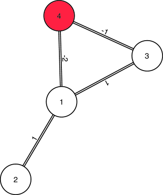
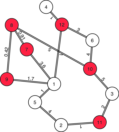
These are all the solutions of Problem 1 that correspond to the chosen values for $P$ and $G$. Note that only $S_{1}$ is Metzler, so that it is the only solution of Problem 2, moreover $S_{1}=S$, where $S$ is in (13). Figures 4 and 5 represent the graphs associated to matrices $S_{1}$ and $S_{2}$. In these and in next graph figures, red nodes denote unmeasured outputs.

Figure 4: Graph representation of $S_{1}$

Figure 5: Graph representation of $S_{2}$

3 Discussion of Problems 2 and 3

Proposition 7 shows that, in the general case, Problem 1 has multiple solutions. We introduced Problems 2 and 3 in order to find specific solutions that satisfy additional properties. Consider a solution of form (6) and assume that $P$ and $G$ are fully known. Then, Problem 2 consists in finding an orthonormal matrix $Q$ such that $T^{-1}\hat{A}T$ is Metzler, or equivalently, finding an orthonormal matrix $\bar{U}$ that satisfies the following equation.

$$\begin{array}[]{ll}\left(\sqrt{G}^{-1}Q^{T}P^{-1}\hat{A}PQ\sqrt{G}\right)_{i,j}\geq 0,\,i\neq j\\ Q=WZ^{+}+\bar{W}\bar{U}\bar{Z}^{T}\end{array}$$ (20)

Note that Problem (20) is non-convex due to the orthonormality constraint on $\bar{U}$ (i.e., $\bar{U}^{T}\bar{U}=I$). Anyway, because of Proposition 7, the dimension of $\bar{U}$ may be small, so that, in some cases, solving (20) can still be a simple task.

Problem 3 adds the requirement of minimizing $\|S\|_{0}$, or, equivalently, minimizing $\|T^{-1}\hat{A}T\|_{0}$. Since the minimization of the zero-norm is a difficult task, as commonly done (see, for instance, [14]), one can use the $1$-norm as a sparsity-promoting objective function, obtaining the following problem:

$$\min_{\bar{U}}\left\|\sqrt{G}^{-1}Q^{T}P^{-1}\hat{A}PQ\sqrt{G}\right\|_{1}\textrm{ such that~{}\eqref{eqn_for_prob_2} holds.}$$ (21)

We can rewrite this problem more explicitly as

$$\begin{array}[]{ll}\underset{\bar{U}}{\min}\left\|\sqrt{G}^{-1}Q^{T}P^{-1}\hat{A}PQ\sqrt{G}\right\|_{1}\\ \textrm{ such that}\\ \left(\sqrt{G}^{-1}Q^{T}P^{-1}\hat{A}PQ\sqrt{G}\right)_{i,j}\geq 0,\,i\neq j\\ Q=WZ^{+}+\bar{W}\bar{U}\bar{Z}^{T}\\ \bar{U}\bar{U}^{T}=I.\end{array}$$ (22)

3.1 Overall algorithm for Problem 3

Leveraging Proposition 4, we can formulate the following algorithm for solving Problem 3. Here the problem data are the identified model $\hat{A}$, $\hat{B}$, $\hat{C}$ and the required input and output matrices $B$, $C$. The final output is given by matrices $P$, $G$ and $\bar{U}$, that give transformation $T$ by (6) and (19).

• Solve Problem (8) in order to find a solution $P$, $G$. Note, that, by Remark 4, in many cases, this solution is unique up to a scaling factor.

• Solve Problem (22) using a nonlinear local search algorithm. In our tests we used different randomly generated initial conditions $\bar{U}_{0}$ for $\bar{U}$ and selected the best solution.

Some remarks are in order on the choice of the initial conditions $\bar{U}_{0}$ for $\bar{U}$. Note that $O(n)$ has two connected components given by $\{e^{S}A,S\in\mathbb{R}^{n\times n}:S=-S^{T},A\in\{I,M\}\}$, where $M$ is the diagonal matrix with all ones on the diagonal apart from a term $-1$ on the first element and $S$ is a skew-symmetric matrix. This comes from the facts the set of skew-symmetric matrices is the Lie algebra of $O(n)$ and that $I$ and $M$ belong to separate connected components of $O(n)$. Hence, we can generate a random initial guess $\bar{U}_{0}$ for $\bar{U}$ by setting $\bar{U}=e^{S}A$, where $S$ is a random skew-symmetric matrix and $A$ is randomly chosen between $I$ and $M$.

3.2 Case of data affected by noise

Real input and output data are affected by noise. In this case, Problem 4 may not have a feasible solution and can be substituted with the following relaxed one.

$$\left\{\begin{array}[]{lll}\min\|\hat{C}VDV^{T}\hat{C}^{T}-CG^{-1}C^{T}\|^{2}+\|\hat{B}^{T}W^{T}D^{-1}W\hat{B}-B^{T}G^{-1}B\|^{2}+\|\hat{C}\hat{B}-CG^{-1}B\|^{2}\\ \textrm{subject to }\\ D>0\\ \Lambda D=D\Lambda\\ G>0\end{array}\right.$$ (23)

Note that if second or third conditions (the requirement on $B$ and $C$) are not present in (4), Problem (23) becomes a convex one. In fact if, for instance, the third conditions is missing, by setting $H=G^{-1}$ the objective function reduces to the convex one $\|\hat{C}VDV^{T}\hat{C}^{T}-CHC^{T}\|^{2}$.

4 Examples

In this section, we consider some examples of larger dimension. In order to test the possibility of recovering the network connections, we randomly generate some autonomous systems in form (1) (the “true” systems) with the following procedure. Given a number of states $n$, we set $G=I$ and $S=-\mathcal{I}K\mathcal{I}^{T}$, where $\mathcal{I}$ is the incidence matrix of a randomly generated graph of $n$ vertices and $K$ is a diagonal matrix of randomly generated conductances (with integer values). Then, we compute a random transformation matrix $\tilde{T}$ and set $\hat{A}=\tilde{T}^{-1}A\tilde{T}$, $\hat{C}=C\tilde{T}$. We consider as output matrix $C$ the projection on the first $m$ components. In all examples, $\hat{A}$ is diagonalizable and condition (12) is satisfied. Hence, $P$ and the first $m$ component along the diagonal of $G$ have only one solution, up to a positive scaling factor. The remaining elements of the diagonal $G$ are undetermined, since they do not appear in Problem (14). For simplicity, we chose the scaling factor such that the reconstructed $G$ is the identity. We solved Problem 3 with the algorithm presented in Section 3.1 and computed the corresponding transformation matrix $T$ and the reconstructed matrix $S$ as $\hat{S}=GT^{-1}\hat{A}T$. Then, we compared matrix $S$ of the true system with the reconstructed one $\hat{S}$, to check if we have been able to correctly reconstruct the network connections. We considered the following two cases.

4.1 Case 1: $n=10$, $m=8$

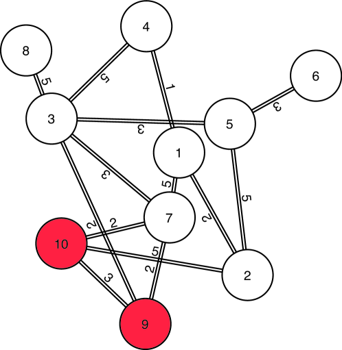
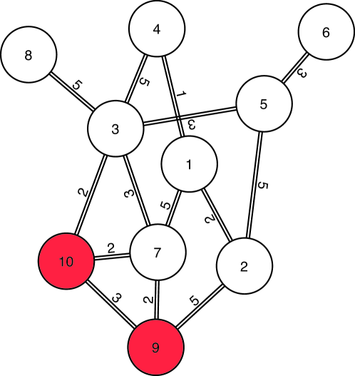
In this example, we do not measure the potential of the last $2$ nodes, that is, matrix $C$ in (4) is the projection on the first $8$ nodes. Generically (see Remark 4), $P$ and $G$ are unique (up to a positive scaling), apart from the last two components of the diagonal of $G$, that are undetermined. By Proposition (7), since $\textrm{ dim}\textrm{ ker }C=2$, the component $Q$ of (6) has multiple solution, parameterized by $\bar{U}\in O(2)$. The algorithm in Section 3.1 allows finding one among such solutions. Figure 6 is the graph associated to $S$ while Figure 7 is the one associated to the reconstructed $\hat{S}$. Note that the two graphs are similar but different. That is, at the end of our procedure, we found a reconstructed system of form (1) which solves Problem 2 (and, approximately, Problem 3), but is different from the true system. This is unavoidable since, by Proposition (7), there are multiple systems that solve Problem 1 and, in general, there may be multiple solutions also of Problems 2 and 3.

Figure 6: Case 1: true connections

Figure 7: Case 1: reconstructed connections

4.2 Case 2: $n=12$, $m=6$

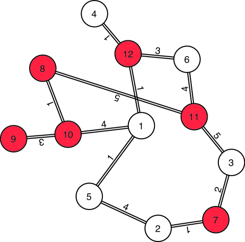
In this example, we measure the potential of $6$ nodes out of $12$. Again, Figure 8 refers to the true matrix $S$ while Figure 9 refers to the reconstructed $\hat{S}$. In this case, $Q$ has multiple solutions parameterized by $\bar{U}\in O(6)$. Again, the reconstructed matrix is different from the true one, namely, at the end of our procedure, we found one of the multiple solutions that solve Problem 2.

Figure 8: Case 2: true connections

Figure 9: Case 2: reconstructed connections

5 Conclusions

Resistive-capacitive (RC) networks are used to model various systems in engineering, physics or biology. We considered a structured identification task, characterized the solution set and presented a possible algorithm for reconstructing the network connections.

Appendix

Proof of Proposition 2

($\Rightarrow$) Assume that (4) has a solution $T$, $S$, $G$, then $GT^{-1}\hat{A}T$ is symmetric, which implies that $GT^{-1}\hat{A}T=T^{T}\hat{A}^{T}T^{-T}G$, which, setting $M=TG^{-1}T^{T}$, implies the first of (7). The second of (4) implies $T^{T}\hat{C}^{T}=C^{T}$, thus $\hat{C}TG^{-1}T^{T}\hat{C}^{T}=CG^{-1}C^{T}$, that is the second of (7). Similarly, the third of (4) implies $\hat{B}^{T}T^{-T}GT^{-1}\hat{B}=B^{T}G^{-1}B$, that is the third of (7). Finally, by the second and third of (4) $CG^{-1}B=\hat{C}TT^{-1}\hat{B}=\hat{C}\hat{B}$.

($\Leftarrow$) Assume that (7) has a solution $M,G$. Let $UU^{T}=M$ be the Cholesky decomposition of $M$. The second, third and fourth conditions of (7) imply that

$$\begin{gathered}\left(\begin{array}[]{ll}\hat{C}U,\\ \hat{B}^{T}U^{-T}\end{array}\right)\left(\begin{array}[]{ll}U^{T}\hat{C}^{T},\quad U^{-1}\hat{B}\end{array}\right)\\ =\left(\begin{array}[]{ll}CG^{-1/2}\\ B^{T}G^{-1/2}\end{array}\right)\left(\begin{array}[]{ll}G^{-1/2}C^{T},\quad G^{-1/2}B\end{array}\right)\,.\end{gathered}$$

Then, by Proposition 8, there exists an orthonormal matrix $Q$ such that $\left(\begin{array}[]{ll}\hat{C}U\\ \hat{B}^{T}U^{-T}\end{array}\right)Q=\left(\begin{array}[]{ll}CG^{-1/2}\\ B^{T}G^{-1/2}\end{array}\right)$, that is

$$\begin{array}[]{ll}\hat{C}UQ=CG^{-1/2}\\ \hat{B}^{T}U^{-T}Q=B^{T}G^{-1/2}\end{array}$$

and, setting $T=UQG^{1/2}$, it follows that $\hat{C}T=C$ and $T^{-1}\hat{B}=B$. Finally, $\hat{A}M=M\hat{A}^{T}$ implies that $\hat{A}=M\hat{A}^{T}M^{-1}=UU^{T}\hat{A}^{T}U^{-T}U^{-1}$ and $GT^{-1}\hat{A}T=GG^{-1/2}Q^{T}U^{-1}\hat{A}UQG^{1/2}=G^{1/2}Q^{T}U^{-1}UU^{T}\hat{A}^{T}U^{-T}U^{-1}UQG^{1/2}$ $=G^{1/2}Q^{T}U^{T}\hat{A}^{T}U^{-T}QG^{-1/2}G=T^{T}\hat{A}^{T}T^{-T}G$. Hence $GT^{-1}\hat{A}T$ is symmetric, which proves the first of (4).

The following is a well-known property of Gram matrices (see for instance Theorem 3.1 of [15].

Proposition 8.

Let $A,B\in\mathbb{R}^{n\times m}$ be such that $A^{T}A=B^{T}B$, then there exists $Q\in O(n)$ such that $A=QB$.

The following proposition is a property of orthonormal transformations.

Proposition 9.

Let $A,B\in\mathbb{R}^{n\times m}$ with $A^{T}A=B^{T}B$ and $\textrm{rank }A=m<n$, let $\bar{A}$, $\bar{B}$ be such that $\bar{A}^{T}\bar{A}=I$, $\bar{B}^{T}\bar{B}=I$, $\bar{B}^{T}B=0$, $\bar{A}^{T}A=0$, and let $Q\in\mathbb{R}^{n\times n}$. Let $\mathcal{R}=\{Q\in O(n):QA=B\}$ and $\mathcal{S}=\{BA^{+}+\bar{B}U\bar{A}^{T},U\in O(n-m)\}$, then $\mathcal{R}=\mathcal{S}$.

Proof.

(Proof that $\mathcal{R}\subset\mathcal{S}$.)

Let $Q\in\mathcal{R}$, then $QA=B$ and $B^{T}Q\bar{A}=(QA)^{T}Q\bar{A}=A^{T}\bar{A}=0$. Hence, $Q\bar{A}$ is orthogonal to $B$ and the image of $Q\bar{A}$ belongs to the image of $\bar{B}$. This implies that there exists a matrix $U$ such that $Q\bar{A}=\bar{B}U$. Moreover, $\bar{A}^{T}Q^{T}Q\bar{A}=I=U^{T}\bar{B}^{T}\bar{B}U$ so that $\bar{B}U\in O(n-m)$. Then, $Q\left(\begin{array}[]{cc}A&\bar{A}\end{array}\right)=\left(\begin{array}[]{cc}B&\bar{B}U\end{array}\right)$. Note that $\left(\begin{array}[]{cc}A^{+}\\ \bar{A}^{T}\end{array}\right)\left(\begin{array}[]{cc}A&\bar{A}\end{array}\right)=I$, so that $\left(\begin{array}[]{cc}A^{+}\\ \bar{A}^{T}\end{array}\right)=\left(\begin{array}[]{cc}A&\bar{A}\end{array}\right)^{-1}$ and $Q=\left(\begin{array}[]{cc}B&\bar{B}U\end{array}\right)\left(\begin{array}[]{cc}A^{+}\\ \bar{A}^{T}\end{array}\right)=BA^{+}+\bar{B}U\bar{A}^{T}$.

(Proof that $\mathcal{S}\subset\mathcal{R}$.)

Let $U\in O(n-m)$, note that

$$\left(\begin{array}[]{cc}B^{T}\\ U^{T}\bar{B}^{T}\end{array}\right)\left(\begin{array}[]{cc}B&\bar{B}U\end{array}\right)=\left(\begin{array}[]{cc}B^{T}B&0\\ 0&I\end{array}\right)=\left(\begin{array}[]{cc}A^{T}A&0\\ 0&I\end{array}\right)=\left(\begin{array}[]{cc}A^{T}\\ \bar{A}^{T}\end{array}\right)\left(\begin{array}[]{cc}A&\bar{A}\end{array}\right),$$

then, by Proposition 8, there exists $Q\in O(n)$ such that $\left(\begin{array}[]{cc}B&\bar{B}U\end{array}\right)=Q\left(\begin{array}[]{cc}A&\bar{A}\end{array}\right)$, so that $QA=B$. Finally, since $\left(\begin{array}[]{cc}A^{+}\\ \bar{A}^{T}\end{array}\right)=\left(\begin{array}[]{cc}A&\bar{A}\end{array}\right)^{-1}$, it follows that $Q=\left(\begin{array}[]{cc}B&\bar{B}U\end{array}\right)\left(\begin{array}[]{cc}A^{+}\\ \bar{A}^{T}\end{array}\right)=BA^{+}+\bar{B}U\bar{A}^{T}$. ∎