Nonobtuse triangulations of PSLGs

Abstract.

We show that any planar straight line graph with $n$ vertices has a conforming triangulation by $O(n^{2.5})$ nonobtuse triangles (all angles $\leq 90^{\circ}$), answering the question of whether any polynomial bound exists. A nonobtuse triangulation is Delaunay, so this result also improves a previous $O(n^{3})$ bound of Eldesbrunner and Tan for conforming Delaunay triangulations of PSLGs. In the special case that the PSLG is the triangulation of a simple polygon, we will show that only $O(n^{2})$ triangles are needed, improving an $O(n^{4})$ bound of Bern and Eppstein. We also show that for any $\epsilon>0$, every PSLG has a conforming triangulation with $O(n^{2}/\epsilon^{2})$ elements and with all angles bounded above by $90^{\circ}+\epsilon$. This improves a result of S. Mitchell when $\epsilon=\frac{3}{8}\pi=67.5^{\circ}$ and Tan when $\epsilon=\frac{7}{30}\pi=42^{\circ}$.

1. Introduction

A planar straight line graph $\Gamma$ (or PSLG from now on) is the disjoint union of a finite number (possibly none) of non-intersecting open line segments (called the edges of $\Gamma$) together with a disjoint finite point set (the vertices of $\Gamma$) that includes all the endpoints of the line segments, but may include other points as well.

If $V$ is a finite point set in the plane, a triangulation of $V$ is a PSLG with vertex set $V$ and a maximal set of edges. If $\Gamma$ is a PSLG with vertex set $V$, then a conforming triangulation for $\Gamma$ is a triangulation of a point set $V^{\prime}$ that contains $V$ and such that the union of the vertices and edges of the triangulation covers $\Gamma$. We allow $V^{\prime}$ to be strictly larger than $V$; in this case $V^{\prime}\setminus V$ are called the Steiner points. We want to build conforming triangulations for $\Gamma$ that have small complexity (the number of triangles used) and good geometry (the shape of each triangle; no angles too large or too small), but these two goals are often in conflict. In this paper, we are interested in finding the best angle bounds on the triangles that allow us to polynomially bound the number of triangles needed in terms of $n$, the number of vertices of $\Gamma$.

If we triangulate a $1\times r$ rectangle into a fixed number of elements, it is easy to check that some angles must tend to zero as $r\to\infty$, so there is no uniform, strictly positive lower angle bound possible, if we want the number of triangles to be bounded only in terms of the number of vertices of the given PSLG. Since the angles of a triangle sum to $180^{\circ}$, if we had an upper bound of $90^{\circ}-\epsilon$ on the angles of a triangulation, then we also have a $2\epsilon$ lower angle bound. Therefore, no upper bound strictly less than $90^{\circ}$ is possible. Thus nonobtuse triangulation (all angles $\leq 90^{\circ}$) is the best we can hope for.

In 1960 Burago and Zalgaller [15] showed that any polyhedral surface has an acute triangulation (all angles $<90^{\circ}$), but without giving a bound on the number of triangles needed. This was used as a technical lemma in their proof of a polyhedral version of the Nash embedding theorem. In 1984 Gerver [25] used the Riemann mapping theorem to show that if a polygon’s angles all exceed $36^{\circ}$, then there exists a dissection of it into triangles with maximum angle $72^{\circ}$ (in a dissection, adjacent triangles need not meet along an entire edge). In 1988 Baker, Grosse and Rafferty [2] again proved that any polygon has a nonobtuse triangulation, and their construction also gives a lower angle bound. As noted above, in this case no complexity bound in terms of $n$ alone is possible, although there is a sharp bound in terms of integrating the local feature size over the polygon. For details, see [7], [40] or the survey [18].

A linear bound for nonobtuse triangulation of point sets was given by Bern, Eppstein and Gilbert [7], and Bern and Eppstein [6] gave a quadratic bound for simple polygons with holes (this is a polygonal region where every boundary component is a simple closed curve or an isolated point). Bern, Dobkin and Eppstein [4] improved this to $O(n^{1.85})$ for convex domains. Bern, S. Mitchell and Ruppert [9] gave a $O(n)$ algorithm for nonobtuse triangulation of simple polygons with holes in 1994 and their construction uses only right triangles. We shall make use of their result in this paper. These and related results are discussed in the surveys [5] and [10]. Other papers that deal with algorithms for finding nonobtuse and acute triangulations include [20], [33], [35], and [37]. Giving a polynomial upper bound for the complexity of nonobtuse triangulation of PSLGs has remained open (e.g., see Problem 3 of [5]). We give such a bound by proving:

Theorem 1.1.

Every PSLG with $n$ vertices has a $O(n^{2.5})$ conforming nonobtuse triangulation.

Maehara [36] showed that any nonobtuse triangulation using $N$ triangles can be refined to an acute triangulation (all angles $<90^{\circ}$) with $O(N)$ elements. A different proof was given by Yuan [55]. In our proof of Theorem 1.1 the triangulation will consist of all right triangles, but the arguments of Maehara or Yuan then show the theorem also holds with an acute triangulation, at the cost of a larger constant in the $O(n^{2.5})$. As noted above, simple examples give a quadratic lower bound for PSLGs (see [6]), so a gap remains between our upper bound and the worst known example. However, this gap can be eliminated in some special cases, e.g.,

Theorem 1.2.

A triangulation of a simple $n$-gon has a $O(n^{2})$ nonobtuse refinement.

This improves a $O(n^{4})$ bound given by Bern and Eppstein [6]. We can also approach the quadratic lower bound if we consider “almost nonobtuse” triangulations:

Theorem 1.3.

Suppose $\theta>0$. Every PSLG with $n$ vertices has a conforming triangulation with $O(n^{2}/\theta^{2})$ elements and all angles $\leq 90^{\circ}+\theta$.

This improves a result of S. Mitchell [38] with upper angle bound $\frac{7}{8}\pi=157.5^{\circ}$ and a result of Tan [47] with $\frac{11}{15}\pi=132^{\circ}$.

A triangulation is called Delaunay if whenever two triangles share an edge $e$, the two angles opposite $e$ sum to $180^{\circ}$ or less. If all the triangles are nonobtuse, then this is certainly the case, so Theorem 1.1 immediate implies

Corollary 1.4.

Every PSLG with $n$ vertices has a $O(n^{2.5})$ conforming Delaunay triangulation.

This improves a 1993 result of Edelsbrunner and Tan [19] that any PSLG has a conforming Delaunay triangulation of size $O(n^{3})$. Conforming Delaunay triangulations for $\Gamma$ are also called Delaunay refinements of $\Gamma$. There are numerous papers discussing Delaunay refinements including [18], [21], [39], [40], [41] and [45]. The argument in this paper does not seem to give a better estimate for Delaunay triangulations than for nonobtuse triangulations, nor does the proof appear to simplify in the Delaunay case. Finding an improvement (either for the estimate or the argument) in the Delaunay case would be extremely interesting.

An alternative formulation of the Delaunay condition is that every edge in the triangulation is the chord of an open disk that contains no vertices of the triangulation. We say the triangulation is Gabriel if every edge is the diameter of such disk. It is easy to check that a nonobtuse triangulation must be Gabriel, so we also obtain a stronger version of the previous corollary:

Corollary 1.5.

Every PSLG with $n$ vertices has a $O(n^{2.5})$ conforming Gabriel triangulation.

Given a finite planar point set $V$, and a point $v\in V$, the Voronoi cell corresponding to $v$ is the open set of points that are strictly closer to $v$ than to any other point of $V$. The union of the boundaries of the all the Voronoi cells is called the Voronoi diagram of $V$. In [42], it is shown that given a nonobtuse triangulation with $N$ elements, one can find a set of $O(N)$ points so that the Voronoi diagram of the point set covers all the edges of the triangulation. Thus we obtain

Corollary 1.6.

For every PSLG $\Gamma$ with $n$ vertices, there is a point set $S$ of size $O(n^{2.5})$ whose Voronoi diagram covers $\Gamma$.

The authors of [42] were interested in a type of machine learning called “nearest neighbor learning”. Given $\Gamma$ and $S$ as in the corollary, and any point $z$ in the plane, we can decide which complementary component of $\Gamma$ $z$ belongs to by finding the element $w$ of $S$ that is closest to $z$; $z$ and $w$ must belong to the same complementary component of $\Gamma$. Thus the corollary says that a partition of the plane by a PSLG of size $n$ can be “learned” from a point set of size $O(n^{2.5})$. This answers a question from [42] asking if a polynomial number of points always suffices.

Acute and nonobtuse triangulations arise in a variety of other contexts. In recreational mathematics one asks for the smallest triangulation of a given object into acute or nonobtuse pieces. For example, a square can obviously be meshed with two right triangles, but less obvious is the fact that it can be acutely triangulated with eight elements but not seven; see [16]. For further results of this type see [23], [24], [26], [27], [28], [29], [30], [31], [43], [56], [57], [58], the 2002 survey [60] and the 2010 survey [59]. There is less known in higher dimensions, but recent work has shown there is an acute triangulation of $\mathbb{R}^{3}$, but no acute triangulation of $\mathbb{R}^{n}$, $n\geq 4$ [14], [32], [34], [50], [51], [52]. Finding polynomial bounds for conforming Delaunay tetrahedral meshes in higher dimensions remains open.

In various numerical methods involving meshes, a nonobtuse triangulation frequently gives simpler and better behaved algorithms. For example, in [54] Vavasis bounds various matrix norms arising from the finite element method in terms of the number $n$ of triangulation elements; for general triangulations his estimate is exponential in $n$, but for nonobtuse triangulations it is only linear in $n$. Other examples where nonobtuse or Delaunay triangulations give simpler or faster methods include: discrete maximum principles [12], [17], [53]; Stieltjes matrices in finite element methods [13], [46]; convenient description of the dual graph [8]; the Hamilton-Jacobi equation [3]; the fast marching method [44]; the tent pitcher algorithm for meshing space-time [1], [48], [49].

The ideas in this paper are used in a companion paper [11] to obtain conforming quadrilateral meshes for PSLGs that have optimal angle bounds and optimal worst case complexity. The precise statement from this paper used in [11] is Lemma 13.1; this follows from a slight modification of the proof of Theorem 1.3. The result obtained in [11] says that every PSLG has an $O(n^{2})$ conforming quadrilateral mesh with all angles $\leq 120^{\circ}$ and all new angles $\geq 60^{\circ}$. The angle bounds and quadratic complexity bound are both sharp.

Many thanks to Joe Mitchell and Estie Arkin for numerous conversations about computational geometry in general and the results of this paper in particular. Also thanks to two anonymous referees for many helpful comments and suggestions on two earlier versions of the paper; their efforts greatly improved the presentation in this version.

In Section 2 we recall a theorem of Bern, Mitchell and Ruppert [9] that connects nonobtuse triangulation to finding Gabriel edges, and we sketch the proof of this result in Section 3. In Section 4 we use their theorem to give a simple proof of Theorem 1.2. In Sections 5-8 we discuss propagation paths, dissections and return regions; these are used in the proofs of both Theorems 1.1 and 1.3. Sections 9–12 give the proof of Theorem 1.3 and Section 13 summarizes facts from the proof that are used in the sequel paper [11]. Section 14 gives an overview of the proof of Theorem 1.1 and Sections 15–21 provide the details.

2. The theorem of Bern, Mitchell and Ruppert

Given a point set $V$ and two points $v,w\in V$, the segment $vw$ is called a Delaunay edge if it is the chord of some open disk that contains no points of $V$ and is called a Gabriel edge if it is the diameter of such a disk (see [22]). We will call a PSLG $\Gamma$ with vertex set $V$ and edge set $E$ Gabriel if every edge in $E$ is Gabriel for $V$. Given a PSLG which is not Gabriel, can we always add extra vertices to the edges, making a new PSLG that is Gabriel? We are particularly interested in the case when $P=T$ is a triangle. See Figure 1.

Figure 1. A triangle that is not Gabriel and one way to add points so that it becomes Gabriel.

The connection between Gabriel triangles and nonobtuse triangulation is given by the following result of Bern, Mitchell and Ruppert [9]. Suppose $T$ is a triangle with three vertices $V_{0}=\{a,b,c\}$ and suppose $V$ is a finite subset of the edges of $T$. Then $T\setminus(V_{0}\cup V)$ is a finite union of segments and we let $V^{\prime}$ denote the midpoints of these segments.

Theorem 2.1.

Suppose we add $N$ points $V$ to the edges of a triangle $T$, so that the triangle becomes Gabriel. Assume further that no point of the interior of $T$ is in more that two of the Gabriel disks. Then the interior of $T$ has a nonobtuse triangulation consisting of $O(N)$ right triangles and the triangulation vertices on the boundary of $T$ are exactly the vertices of $T$ and the points in $V$ and $V^{\prime}$.

This follows from the proof in [9], but this precise statement does not appear there, so in the next section we will briefly describe now to deduce Theorem 2.1 from the arguments in [9].

We say that one triangulation ${\mathcal{T}}_{1}$ is a refinement of another triangulation ${\mathcal{T}}_{2}$, if each triangle in ${\mathcal{T}}_{2}$ is a union of triangles in ${\mathcal{T}}_{1}$. If $\Gamma$ is a PSLG that is a triangulation and we add enough points to the edges of $\Gamma$ to make every triangle Gabriel, then the resulting nonobtuse refinements of each triangle agree along any common edges (the set of boundary vertices is $e\cap(V\cup V^{\prime})$ for both triangles with edge $e$). Thus we get:

Corollary 2.2.

Suppose that $\Gamma$ is a planar triangulation with $n$ elements, and that we can add $N$ vertices to the edges of $\Gamma$ so that every triangle becomes Gabriel. Then $\Gamma$ has a refinement consisting of $O(n+N)$ right triangles.

It is fairly easy to see that we can always add a finite number of vertices and make each triangle Gabriel. Thus nonobtuse refinement of a triangulation is always possible, but the difficulty is to bound $N$ in terms of $n$. Since any PSLG with $n$ vertices can be triangulated using $O(n)$ triangles (and the same vertex set), Theorem 1.1 is reduced to

Theorem 2.3.

Given any triangulation with $n$ elements we can add $O(n^{2.5})$ vertices to the edges so that every triangle becomes Gabriel.

We will prove this for general planar triangulations later in the paper. We start with the simpler case of triangulations of simple polygons (Theorem 1.2) in Section 4. The key feature of this special case is that the elements of such a triangulation form a tree under adjacency (sharing an edge); this fails for general triangulations, and dealing with this failure is the main goal of this paper.

In Theorem 2.3 we only need to check that each triangle becomes Gabriel, not that the point set is Gabriel for the whole triangulation. The difference is that in the first case if we take a disk $D$ with an edge $e$ as its diameter, we only have to make sure that $D$ does not contain any vertices belonging to the two triangles that have $e$ on their boundary. In the second case, we would have to check that $D$ does not contain any vertices at all. This apparently stronger condition follows from the weaker “triangles-only” condition, but we don’t need this fact for the proof of Theorem 1.1.

3. Sketch of the proof of Theorem 2.1

As noted above, Theorem 2.1 is due to Bern, Mitchell and Ruppert in [9], but the precise result is not given in that paper. For the convenience of the reader, we briefly sketch how our statement is deduced using the argument in [9].

The basic idea in [9] is to pack the interior of a polygon $P$ (which in our case is just a triangle $T$) with disks until the remaining region is a union of pieces that are each bounded by three or four circular arcs, or a segment lying on the polygon’s boundary. These are called the remainder regions.

Each remainder region $R$ is associated to a simple polygon $R^{+}$, called the augmented region of $R$ as follows. Each circular arc in the boundary of $R$ lies on some circle,and we add to $R$ the sector of the circle subtended by this arc. Doing this for each boundary arc of $R$ gives the polygon $R^{+}$. See Figure 2.

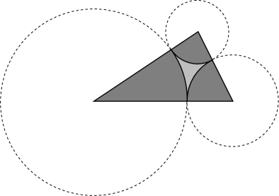
Figure 2. The light gray is a 3-sided remainder region $R$ and the dark gray is the corresponding augmented region $R^{+}$.

The augmented regions decompose the original polygon into simple polygons and the authors of [9] show how each augmented region can be meshed with right triangles. Moreover, the mesh of $R^{+}$ only has vertices at the vertices of $R^{+}$ (the centers of the circles), the endpoints of the boundary arcs (the tangent points between disks) or on the straight line segments that lie on the boundary of $P=T$.

We modify their construction first placing the Gabriel disks along the edge of the triangle, as shown in Figure 3. The disk packing construction of [9] will only be applied to the part of the triangle outside the Gabriel disks, hence none of the remainder regions that are formed will have straight line boundary segments on the boundary of $T$.

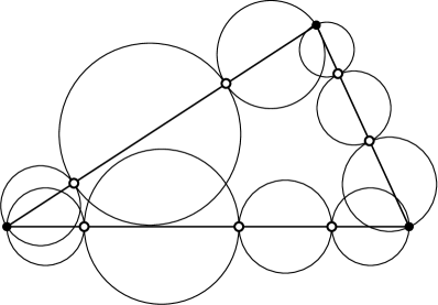
Figure 3. The white points are the set $V$ that makes the triangle $T$ Gabriel. The Gabriel disks may intersect in pairs, but we assume that no three of them intersect.

Whenever two Gabriel disks overlap, we place a small disk $D$ near each of the intersection points of their boundaries. The disk $D$ is tangent to both overlapping disks and its interior is disjoint from all the Gabriel disks. See Figures 4 and 5 for two situations where this can occur: the boundaries of the Gabriel disks (which we call the Gabriel circles) either have two intersections inside $T$ or they have just one intersection inside $T$.

Figure 4 shows what happens when the boundaries intersect at two points. We place two disks near the intersections points (the dashed disks in the figure), and we form a quadrilateral by connecting the centers of the four circles. This quadrilateral is then meshed with 16 right triangles as shown in the figure. The overall structure is shown on the left, and an enlargement is shown on the right. The black point on the right where six triangles meet is the common intersection point of three lines: the line $L_{0}$ through the two intersection points of the Gabriel circles, and the two tangent lines $l_{1},l_{2}$ between the dashed disk and the the Gabriel disks. It is proven in [9] that these three lines meet at a single point, as shown. The center of the dashed circle in Figure 4 is not necessarily on $L_{0}$ (although it appears this way in the figure). Figure 5 shows the case when two Gabriel circles have one intersection inside $T$ (and the other is at vertex of $T$). The proof that all the triangles are right is fairly evident (see [9]).

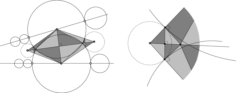
Figure 4. Gabriel disks whose boundaries intersect twice inside $T$. We add tangent disks as shown (dashed) and triangulate as shown. The picture on the right shows more detail near one of the added disks. The point where six triangles meet is the intersection of the line through the intersection points of the Gabriel circles and the two tangent lines between the added disk and the Gabriel disks.

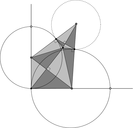
Figure 5. Figure 5 is analogous to Figure 4, but shows that case when two Gabriel circles have a single intersection inside $T$ (the other is at a vertex of $T$). In this case, the mesh is a sub-picture of the previous case and only uses 10 right triangles.

From this point the proof follows [9]. Lemma 1 of the paper shows that we can add disjoint disks until all the remainder regions have three or four sides and that the number of disks added is comparable to the number of Gabriel disks we started with. See Figure 6.

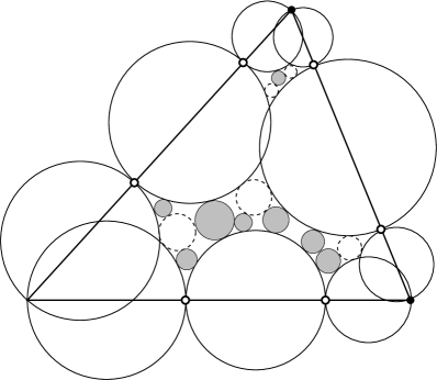
Figure 6. After adding the disks (dashed) tangent to the intersecting Gabriel disks, we pack the remaining region with disjoint disks (gray) until only circular arc regions with three or four sides remain. This step and the rest of the proof follow the proof in [9] exactly.

Because of the Gabriel disks, none of the remainder regions have straight line boundary arcs, so all the augmented regions are meshed by right triangles whose vertices are either interior to $T$ or lie in the set $V$ or in the set $V^{\prime}$ (the centers of the Gabriel disks) and every such point is used. This gives Theorem 2.1.

4. Proof of Theorem 1.2

A PSLG $\gamma$ is a simple polygon if it is a simple closed Jordan curve. Suppose $\gamma$ is a simply polygon and $\{T_{k}\}_{1}^{N}$ is a triangulation of $\gamma$ with no Steiner points. The union of the edges and vertices of the triangulation is the PSLG $\Gamma$ in Theorem 1.2. For each triangle $T_{k}$, let $C_{k}$ be the inscribed circle and let $T_{k}^{\prime}\subset T_{k}$ be the triangle with vertices at the three points where $C_{k}$ is tangent to $T_{k}$. Note that the arcs between points of $C_{k}$ all have angle measure $<\pi$, so $T_{k}^{\prime}$ must be acute. These vertices of $T_{k}^{\prime}$ will sometimes be called the cusp points of $T_{k}$. See Figures 7 and 8.

Figure 7. The definition of $C_{k}$ and $T_{k}^{\prime}$.

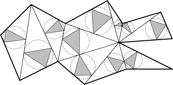
Figure 8. A triangulation $\{T_{k}\}$ of a simple polygon, the inscribed circles (dashed) and triangles $\{T_{k}^{\prime}\}$ (shaded).

Also note that $T_{k}\setminus T_{k}^{\prime}$ consists of three isosceles triangles, each with its base as one side of $T_{k}^{\prime}$ and its opposite vertex a vertex of $T_{k}$. Foliate each isosceles triangle with segments that are parallel to its base (foliate simply means to write a region as a disjoint union of curves). We call these P-segments (since they are “parallel” to the base and they will also allow us to “propagate” certain points through the triangulation).

Given a vertex $v$ of some $T_{k}^{\prime}$, this point is either on $\gamma$ (the boundary of the triangulation) or it is on the side of some other triangulation element $T_{j}$, $j\neq k$. In the first case do nothing. In the second case, either $v$ is also a vertex of $T_{j}^{\prime}$ or it is not. In the first case, again do nothing. In the second case, build a polygonal path whose first edge is the $P$-segment in $T_{j}$ that has $v$ as one endpoint. The other endpoint is a point $w$ on a different side of $T_{j}$. If $w$ is on $\gamma$, or is a vertex of some $T_{i}^{\prime}$, $i\neq j$, then end the polygonal arc at $w$. Otherwise, $w$ is on the side of some third triangle $T_{i}$ and we can add the $P$-segment in $T_{i}$ that has one endpoint at $w$. See Figures 9 and 10.

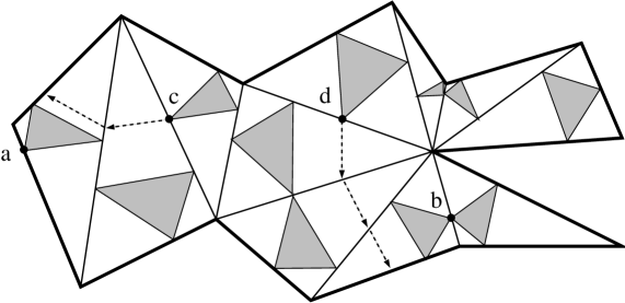
Figure 9. A cusp point (vertex of a shaded triangle) can either be on $\gamma$ (the boundary of the triangulation), can be a vertex of another shaded triangle, or neither. In the last case we can “propagate” the vertex using a $P$-segment and continue the process until one the first two conditions holds. Vertices $a$ and $b$ represent the first two possibilities and vertices $c$ and $d$ both represent the third case; the dashed lines show how these points propagate until they hit the boundary.

Figure 10. Here is the same triangulation as in Figure 9 with all cusp points propagated until they terminate. This refines the triangulation into acute triangles (shaded) and isosceles triangles and trapezoids (white). We claim the new vertices make all the original triangles Gabriel.

We continue in this way, adding $P$-segments to our polygonal path until we either reach a point on the boundary of the triangulation or hit a point that is the vertex of some triangle $T_{m}^{\prime}$. We call the path formed by adjoining $P$-segments a $P$-path. Since our triangles come from a triangulation of a simple polygon, they form a tree under edge-adjacency and so the $P$-paths starting at the three vertices of $T_{k}^{\prime}$ must cross distinct triangles and hence can use at most $n-1$ segments altogether. Thus every $P$-path must terminate and all the $P$-paths formed by starting at all vertices of all the $\{T_{k}^{\prime}\}$ can create at most $n(n-1)$ new vertices altogether.

Lemma 4.1.

The set $U$ of vertices created by these $P$-paths crossing edges of $\{T_{k}\}$ makes every triangle Gabriel.

Proof.

Note that $U$ contains every vertex of every $T_{k}^{\prime}$ and we also include in $U$ the all vertices of all the $T_{k}$’s. To prove the lemma, consider a segment $e$ that is a connected component of $T_{k}\setminus U$ (so $e$ is a diameter of one of our Gabriel disks). Since $U$ contains the vertices of $T_{k}^{\prime}$, $e$ lies on a non-base side of one of the three isosceles triangles inside $T_{k}$. If we reflect $e$ over the symmetry axis of this isosceles triangle we get an edge $e^{\prime}$ on the other non-base side. Moreover, $e^{\prime}$ is also one of the edges created by adding $U$ to the triangulation, and the disks $D$, $D^{\prime}$ with diameters $e$ and $e^{\prime}$ respectively, are reflections of each other through the symmetry line of the isosceles triangle. Thus the boundaries of $D$ and $D^{\prime}$ intersect, if at all, on the line of symmetry, so $D\cap e^{\prime}\subset e^{\prime}$ and $D^{\prime}\cap e\subset e$. In particular, the open disk $D$ does not contain the endpoints of $e^{\prime}$ and vice versa. This implies $D$ can’t contain any of the points of $U$ that lie on the same side of $T_{k}$ as $e^{\prime}$. Clearly $D$ does not contain any points of $U$ on the side of $T_{k}$ containing $e^{\prime}$. Finally, $D$ does not contain any points of $U$ that are on the third side of $T_{k}$ because $D$ is contained in the disk $D^{\prime\prime}$, centered at the vertex of $T_{k}$ where the sides containing $e$ and $e^{\prime}$ intersect and passing through two vertices of $T_{k}^{\prime}$, and this disk does not hit the third side of $T_{k}$. See Figure 11. ∎

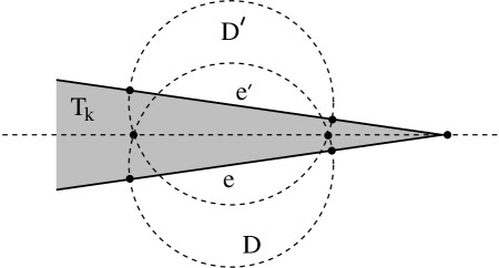
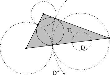
Figure 11. The points where propagation paths cross triangle edges define Gabriel edges in each triangle. Note that at most two Gabriel disks can intersect when the cusp points are included in set of endpoints (the set $V$ in Theorem 2.1).

This argument also shows that two Gabriel disks can only intersect if they lie on different non-base sides of one of the three isosceles sub-triangles. Thus no three disks can intersect and the condition in Theorem 2.1 is automatically satisfied whenever the set $V$ contains the vertices of $T_{k}^{\prime}$ for every $k$.

Thus for each triangle $T_{k}$, the points $U\cap T_{k}$ makes $T_{k}$ Gabriel. By Theorem 2.1, $T_{K}$ has a nonobtuse triangulation with only these boundary vertices and using $O(\#(U\cap T_{k}))$ triangles. These triangulations fit together to form a nonobtuse refinement of the original triangulation of size $O(\#(U)+n)=O(n^{2})$, which proves Theorem 1.2.

We can make a slight improvement to the algorithm above. As we propagated each vertex, we could have stopped whenever the path encountered any isosceles triangle with angle $\geq 90^{\circ}$. In this case, the Gabriel condition will be satisfied no matter how we add points to a non-base sides of the isosceles triangle, since the corresponding disks don’t intersect the other non-base side of the triangle. See Figure 12. In some cases this might lead to a smaller nonobtuse triangulation. This observation will also be used later in the proof of Theorem 1.1, when it will be convenient to assume we are dealing only with isosceles triangles that are acute.

Figure 12. $P$-paths can be stopped when they hit an isosceles triangle with angle $\geq 90^{\circ}$ since the corresponding Gabriel disks can’t hit the other sides of the triangle.

5. Dissections and quadrilateral propagation

We now start to prepare for the proofs of Theorems 1.1 and 1.3. The definitions and results in this and the next three sections will be used in both proofs.

Suppose $\Omega$ is a domain in the plane (an open connected set). We say $\Omega$ has a polygonal dissection if there are a finite number of simple polygons (called the pieces of the dissection) whose interiors are disjoint and contained in $\Omega$ and so that the union of their closures covers the closure of $\Omega$. A mesh is a dissection where any two of the closed polygonal pieces are either (1) disjoint or (2) intersect in a point that is a vertex for both pieces or (3) intersect in a line segment that is an edge for both pieces. See Figure 13 for an example. A dissection is also called a non-conforming mesh. A vertex of one dissection piece that lies on the interior of an edge for another piece is called a non-conforming vertex. If there are no such vertices, then the dissection is actually a mesh.

Figure 13. On the left is a polygon dissected into quadrilaterals and triangles and on the right is the standard propagation of the non-conforming vertices until the propagation paths leave the polygon. If all the paths terminate, this gives a mesh, as described in the text.

Given any convex quadrilateral with vertices $a,b,c,d$ (say in counterclockwise order), there is a unique affine map from $[a,b]$ to $[c,d]$ that takes $a$ to $d$ and $b$ to $c$. A propagation segment in the quadrilateral is a segment connecting a point in $[a,b]$ to its affine image point in $[c,d]$ (or connecting a point in $[b,c]$ to its affine image in $[d,a]$ under the analogous map for that pair of sides). See Figure 14. In a triangle $A,B,C$ with marked vertex, say $A$, propagation paths either connect points on $[A,B]$ to their linear images on $[A,C]$ or they connect any point on $[B,C]$ to the single point $A$ (this is what we would get if we think of the triangle as a degenerate quadrilateral $A,B,C,D$ with $A=D$, i.e., one side of length zero).

Given $\theta>0$, we say a quadrilateral is $\theta$-nice if all the angles are within $\theta$ of $90^{\circ}$. In this paper we will always assume $\theta<90^{\circ}$ so the quadrilateral is convex. We say a triangle with a marked vertex is $\theta$-nice if the two unmarked vertices have angles that are within $\theta$ of $90^{\circ}$.

Figure 14. Standard propagation segments for a quadrilateral and a triangle with a marked vertex (A). In both cases, “$\theta$-niceness” is preserved by cutting a piece into sub-pieces by such segments.

Lemma 5.1.

Suppose $\theta<90^{\circ}$ and that $Q$ is a $\theta$-nice quadrilateral. If $Q$ is sub-divided by a propagation line, then each of the resulting sub-quadrilaterals is also $\theta$-nice.

Proof.

Set $a_{t}=(1-t)a+tb$ and $c_{t}=(1-t)d+tc$. Let $I_{t}=[a_{t},c_{t}]$ be the segment connecting these points and let $\theta(t)$ be the angle formed by the segments $[a,b]$ and $I_{t}$. It suffices to show this function is monotone in $t$. If it were not monotone, then there would be two distinct values of $s,t\in[0,1]$ where $I_{s}$ and $I_{t}$ were parallel. Because both endpoints move linearly in $t$, this implies $I_{r}$ is parallel to $I_{s}$ for all $s\leq r\leq t$. Because $\theta(t)$ is analytic in $t$, this means it is constant on $[0,1]$. Thus $\theta$ is either strictly monotone or is constant; in either case it is monotone, as desired. ∎

Similarly (but more obviously), when a $\theta$-nice triangle is cut by such a propagation segment (of either type) the resulting pieces are $\theta$-nice quadrilaterals or $\theta$-nice triangles.

Lemma 5.2.

Suppose $\Omega$ has a dissection into $\theta$-nice pieces (triangles and quadrilaterals). Suppose that every non-conforming vertex can be propagated so that it reaches the boundary of $\Omega$ or hits another vertex after a finite number of steps. Then the resulting paths cut the $\theta$-nice dissection pieces into $\theta$-nice triangles and quadrilaterals that mesh $\Omega$.

The proof is evident since when we are finished, there are no vertices that are in the interior of any edge of any piece. See Figure 13. What is not so clear is whether, in general, the propagation paths have to end; in the proof of Theorem 1.2 every propagation path did end within a fixed number of steps, but in general, the paths may never terminate (see Figure 15) or may only terminate only after a huge number of steps. Later in this paper we discuss two ways of “bending” the standard propagation paths so that they terminate within a certain number of steps, and so that the pieces formed satisfy certain geometric conditions.

      

      

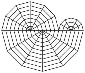
Figure 15. The upper lefts shows an isosceles dissection of a region. The horizontal segment is $S=[0,1]$ and the six vertices shown on this segment are (left to right) $0,\frac{\alpha}{2},\frac{1}{2},\alpha,\frac{1+\alpha}{2},1$. A path started at a point $x\in S$ will visit $x-\alpha\mod 1$ after propagating once through the upper half-plane and once through the lower half-plane. The upper right and lower left pictures show a path after 2 visits to the lower half-plane and 50 visits for $\alpha=1/\sqrt{2}$. If $\alpha$ is irrational, then the propagation path becomes dense in the dissected region. When $\alpha$ is rational, the propagation paths either connect non-conforming vertices or are loops; the connecting paths give a mesh but there is no uniform bound on the number of elements. The connecting paths for $\alpha=.7$ are shown at lower right; the resulting tubes are filled with $P$-loops.

6. Isosceles dissections

Next we discuss a special type of polygonal dissection. An isosceles triangle is a triangle $T$ with a marked vertex $v$ so that the two sides adjacent to $v$ have equal length. An equilateral triangle can be considered as isosceles in three ways, but we assume that if such triangles occur, a vertex is specified.

The side opposite $v$ is called the base of $T$ and the other two sides are the non-base sides of $T$. The angle of an isosceles triangle will always refer to the interior angle at the vertex opposite the base edge. A $P$-segment is a segment in $T$ with endpoints on the non-base sides that is parallel to the base. This is a special case of the propagation segments for marked triangles in the previous section. We require the interior of the segment to be in the interior of $T$, so the base itself is not a $P$-segment. We say a triangle is $\theta$-nice if all its angles are bounded above by $90^{\circ}+\theta$.

An isosceles trapezoid is a quadrilateral that has a line of symmetry that bisects opposite sides. This is equivalent to saying that there is at least one pair of parallel sides (called the base sides) that have the same perpendicular bisector and the other pair of sides (the non-base sides) have the same length as each other. We allow rectangles, but in this case we specify a pair of opposite sides as the base sides. The angle of an isosceles trapezoid is the angle made by the lines that contain the two non-base sides; we take this to be zero if these sides are parallel (when the trapezoid is a rectangle). The vertex of the trapezoid is the point where these same lines intersect (in the case when they are not parallel; otherwise we say the vertex is at $\infty$). See Figure 16. We say a quadrilateral is $\theta$-nice if all its interior angles are between $90^{\circ}-\theta$ and $90^{\circ}+\theta$ (inclusive). This is the same as saying the angle of the trapezoid is $\leq\theta$.

Figure 16. An isosceles trapezoid. The base sides are vertical in this picture. The vertex is the point $v$ and the width $w$ is the length of the non-base sides. The angle of the trapezoid is $\theta$.

As with isosceles triangles, we can define $P$-segments in an isosceles trapezoid as segments in the trapezoid that are parallel to the base sides (again, these correspond to propagation segments for quadrilaterals). A $P$-path is a simple polygonal arc formed by adjoining $P$-segments end-to-end.

An isosceles piece is either an isosceles triangle or an isosceles trapezoid. We will use this term when it is unimportant which type of shape it is. When referring to a base side of an isosceles piece we mean either base side for a trapezoid and the base side or the opposite vertex for a triangle; the vertex is considered as a segment of length $0$, so when we refer to the length of the smaller base side of an isosceles piece, we mean zero if the piece is a triangle.

A $Q$-segment in an isosceles triangle is a segment joining a point of the base to the vertex opposite the base. The two non-base sides do count as $Q$-segments, and we shall also call these the $Q$-sides of the isosceles triangle. A $Q$-segment for an isosceles trapezoid is a propagation segment that connects the base sides of the trapezoids. As with triangles, we count the non-base sides as $Q$-segments and call these the $Q$-sides of the trapezoid. The width of the piece is the length of a $Q$-side (both $Q$ sides have the same length). It might be more natural to define the width as the distance between the base sides, but the definition as given will simplify matters when we later join isosceles pieces to form tubes.

Suppose that $\Omega$ is a domain in the plane (an open connected set). As might be expected, an isosceles dissection of $\Omega$ is a finite collection of disjoint, open isosceles triangles and trapezoids contained in $\Omega$, so that the union of their closures covers all of $\Omega$. However, we also require that when two pieces have sides with non-trivial intersection, these sides are both $Q$-sides. We do this so that in an isosceles dissection, a $P$-path can always be continued unless the path hits a vertex of the dissection, or hits the boundary of the dissected region. A $\theta$-isosceles dissection is an isosceles dissection where every piece is $\theta$-nice.

For example, Figure 8 in Section 4 shows a triangulated polygon. Let $\Omega$ be the part of interior of the polygon with the (closed) shaded triangles removed; the remaining white region it is a union of isosceles triangles that only meet along non-base sides. Thus $\Omega$ has an isosceles dissection; note that it is not a mesh since the isosceles triangles do not always meet along full edges. When we remove the $P$-paths generated by propagating the vertices of the central triangles, we obtain a mesh into isosceles triangles and trapezoids (as required by Lemma 5.2). See Figure 10. We call this an isosceles mesh.

Figure 15, upper left, shows an isosceles dissection of a region using 18 triangles. In that example, if $\alpha$ is irrational, then the $P$-paths never hit the boundary of the region and can continue forever without terminating. For $\alpha$ rational the $P$-paths starting at non-conforming vertices terminate at other non-conforming vertices and these paths create an isosceles mesh. However, the number of mesh elements depends on the choice of $\alpha$ and may be arbitrarily large.

In Figure 17, we show an isosceles dissection using only trapezoids, and an isosceles mesh generated by propagating non-conforming vertices along $P$-paths.

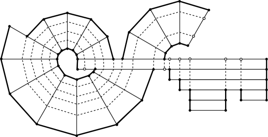
Figure 17. A domain $W$ dissected by isosceles trapezoids and a mesh generated by propagating non-conforming vertices along $P$-paths. The $P$-sides of the trapezoids are drawn thicker.

A chain in a dissection is a maximal collection of distinct pieces $T_{1},\dots,T_{k}$ so that for $j=1,\dots k-1$, $T_{j}$ and $T_{j+1}$ share a $Q$-side (the sides are identical, not just overlapping). If a piece in the dissection does not share $Q$-side with any other piece, we consider it as a chain of length one. For example, the dissection in Figure 17 has chains of length 2,4, 5 and 7 and four chains of length 1. The $Q$-ends of a chain are the $Q$-side of $T_{1}$ not shared with $T_{2}$, and the $Q$-side of $T_{k}$ not shared with $T_{k-1}$. When $T_{1}$ and $T_{k}$ also share a $Q$-side, then the chain forms a closed loop. We will call this a closed chain (this case is not of much interest to us since no propagation paths will ever occur inside such a closed chain.)

Suppose $T$ is an isosceles piece. Given $\theta>0$, a $\theta$-segment is a segment in $T$ with one endpoint on each non-base side, and so that the segment is within angle $\theta$ of being parallel to the base. We allow one endpoint of a $\theta$-segment to be a vertex of $T$, but the interior of the segment must be contained in the interior of $T$, so we don’t consider base sides of $T$ to be $\theta$-segments. A $\theta$-path is a polygonal arc made up of $\theta$-segments joined end-to-end. We shall sometimes refer to this as a $\theta$-bent path. Note that if $T$ is an $\theta$-nice isosceles piece that is cut by a $P$-segment, then it is cut into two $\theta$-nice isosceles pieces. If it is cut by a $\theta$-segment, then we get two pieces (triangles or quadrilaterals) that are $2\theta$-nice (but not isosceles unless $\theta=0$). See Figure 18.

           

Figure 18. A $\theta$-segment (dashed) makes angle at most $\theta$ with $P$-segments (solid). A $\theta$-path is made up out of $\theta$-segments.

We say that a finite set of points on the $Q$-sides of an isosceles piece make that piece Gabriel if the following holds. Each $Q$ side is split into several segments by these points and we require that the open disks with these segments as diameters do not contain any of the added points or corners of the piece. See Figure 19.

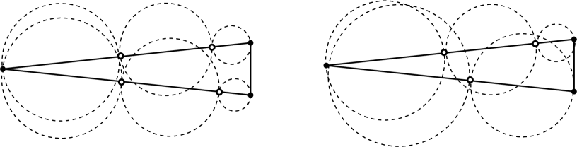
Figure 19. On the left the points make this piece Gabriel, on the right they do not.

7. Tubes

Two $P$-paths $\gamma_{0},\gamma_{1}$ are parallel if each point of $\gamma_{0}$ can be connected to a point of $\gamma_{1}$ by a $Q$-segment (equivalently, the paths cross the same sequence of isosceles pieces, in the same order). A tube in $\Omega$ is the union of two parallel $P$-paths $\gamma_{0},\gamma_{1}$ and all the $Q$ segments that connect the first to the second. The $P$-paths $\gamma_{0}$, $\gamma_{1}$ are called the $P$-sides or $P$-boundaries of the tube. See Figure 20.

Suppose the endpoints of $\gamma_{0}$ and $\gamma_{1}$ are $\{x_{0},y_{0}\}$ and $\{x_{1},y_{1}\}$ respectively and that $[x_{0},x_{1}]$ and $[y_{0},y_{1}]$ are $Q$-segments. These segments are called the ends or $Q$-ends of the tube. These may or may not be disjoint segments. The two ends of a tube have the same length, and this common length of each of the two $Q$-ends is called the width of the tube (a tube can be thought of as a union of isosceles pieces, all of the same width, joined end-to-end along their $Q$-sides). The points $\{x_{0},y_{0},x_{1},y_{1}\}$ are the corners of the tube (although in some cases, these need not be four distinct points in the plane, e.g. pure spirals that we will discuss later). Opposite corners of a tube mean either the pair $\{x_{0},y_{1}\}$ or the pair $\{x_{1},y_{0}\}$. A maximal width tube is the union of all $P$-paths parallel to a given one. If a tube is maximal width, then each of the $P$-path boundaries contains segments that are bases for at least one piece that the tube crosses (otherwise we could widen the tube). See Figure 20.

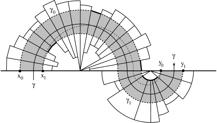
Figure 20. Given a $P$-path $\gamma$ that returns to the same $Q$-segment, there is an associated widest return region consisting of all parallel paths. The $P$-boundary of this tube consists of the two curves $\gamma_{0},\gamma_{1}$; by maximality, each must contain a base edge of a dissection piece (highlighted with darker edges in the figure). The points $x_{0},y_{1}$ form one pair of opposite corners; $x_{1},y_{0}$ the other pair. We are interested in joining opposite corners by a $\theta$-path crossing the tube (dashed curve connecting $x_{1}$ to $y_{0}$).

We say a path strictly crosses a tube if it is contained in the tube and has one endpoint on each $Q$-end. We say a path crosses a tube if it contains a sub-path that strictly crosses the tube. The $P$-paths that strictly cross a tube can be parameterized as $\gamma_{t}$ with $t\in[0,1]$ where $\gamma_{0}$ and $\gamma_{1}$ are the $P$-sides of the tube as discussed above and $\gamma_{t}$ has endpoints $x_{t}=(1-t)x_{0}+tx_{1}$ and $y_{t}=(1-t)y_{0}+ty_{1}$. Moreover

$$\ell(\gamma_{t})=(1-t)\ell(\gamma_{0})+t\ell(\gamma_{1}),$$

where $\ell(\gamma)$ denotes the length of a path $\gamma$. This formula is obvious for tubes that have a single isosceles piece, and it follows in general since a sum of affine functions is affine. The path with $t=1/2$ is called the center path of the tube. Note that

(7.1) $$\ell(\gamma_{1/2})=\frac{1}{2}(\ell(\gamma_{0})+\ell(\gamma_{1})).$$

The length $\ell(T)$ of a tube $T$ is the minimum length of the two $P$-sides, i.e.,

$$\ell(T)=\min(\ell(\gamma_{0}),\ell(\gamma_{1})).$$

It is possible for a tube to have length zero, e.g., when all the pieces are triangles with a common vertex. See the left side of Figure 21.

The length of an isosceles piece is the length of its shorter base edge (zero for triangles). If a tube $T$ is made up of isosceles pieces $\{T_{k}\}$ then it is possible to have both $\ell(T)>0$ and and $\ell(T_{k})=0$ for all $k$. See the right side of Figure 21. We define the minimal-length of a tube to be

$$\tilde{\ell}(T)=\sum\ell(T_{k}),$$

i.e., we sum over the minimal base length for each piece of the tube, whereas $\ell(T)$ is defined by summing over all segments in one $P$-boundary of the tube or all segments in the other. Clearly $\tilde{\ell}(T)\leq\ell(T)$.

       

Figure 21. On the left is a tube of length zero. On the right is a tube with positive length, but zero minimal-length.

As noted above, it is possible to have both $\tilde{\ell}(T)=0$ and $\ell(T)>0$. However, if we split a tube into two parallel tubes using the center path then this cannot happen for either sub-tube:

Lemma 7.1.

Let $Q$ be a tube and $Q_{1}$, $Q_{2}$ the parallel sub-tubes obtained by splitting $Q$ by its center path $\gamma$. Then $\ell(Q)\leq\ell(Q_{1})$ and $\ell(Q)\leq 4\tilde{\ell}(Q_{1})$.

Proof.

Let $\gamma_{1}$ be the common $P$-boundary of $Q$ and $Q_{1}$, and $\gamma_{2}$ the common $P$-boundary of $Q$ and $Q_{2}$. See Figure 22. By Equation (7.1), the center path $\gamma$ of $Q$ has length between the lengths of $\gamma_{1}$ and $\gamma_{2}$. Thus

$$\ell(Q)=\min(\ell(\gamma_{1}),\ell(\gamma_{2}))\leq\min(\ell(\gamma_{1}),\ell(\gamma))=\ell(Q_{1}).$$

This is the first inequality in the lemma.

Figure 22. The tube $Q$ is split into two parallel tubes $Q_{1},Q_{2}$, by its mid-path $\gamma$.

To prove the second inequality, suppose $L=\ell(Q)$ is the length of the tube $Q$ and $\gamma_{1}$ is the $P$-boundary shared by $Q$ and $Q_{1}$. The length of $\gamma_{1}$ is the sum of the lengths of its segments and we group this sum into two parts, depending on whether or not the segments are the longer or shorter base sides of the corresponding isosceles pieces in $Q$ (if the piece has equal length bases, its makes no difference in which sub-sum we place the segment). Call the two sums $L_{0}$ and $L_{1}$ where these give the sums over the shorter edges and longer edges respectively. By definition $L=L_{0}+L_{1}$. If $L_{0}\geq\frac{1}{2}L$, then the short sides of $Q$ (and hence the short sides of $Q_{1}$) add up to at least $\frac{1}{2}L_{1}$. So in this case $\tilde{\ell}(Q_{1})\geq\frac{1}{2}L\geq\frac{1}{4}L$, as desired. If $L_{0}<\frac{1}{2}L$, then $L_{1}>\frac{1}{2}L$ and hence the corresponding mid-segments of the pieces add up to $\frac{1}{4}L$ (since the mid-segment has length as least half the longer base side). But these mid-segments are the shorter base sides of pieces in $Q_{1}$, so again $\tilde{\ell}(Q_{1})\geq\frac{1}{4}L$, as desired. This proves the lemma. ∎

The $P$-segments give an identification between the non-base sides of an isosceles piece that preserves length. The displacement of a $\theta$-segment $[a,b]$ is $|p-b|$ where $[a,p]$ is a $P$-segment. It is easy to check that this is unchanged if we reverse the roles of $a$ and $b$. Similarly, the two ends of a tube are identified by an isometry induced by the parallel $P$-paths defining the tube. The displacement of a path that strictly crosses the tube is $|b-p|$ where $a,b$ are the endpoints of the path and the $P$-path starting at $a$ hits the other end at $p$. The most important estimates in the remainder of the paper involve how much displacement a path can have, given that it satisfies certain limitations on its “bending” across each isosceles piece. For Theorem 1.3, the bending is bounded by a fixed angle $\theta$, and for Theorem 1.1 the amount of bending depends on the piece and is determined by the Gabriel condition.

8. Return regions

In this section we introduce a collection of regions, one of which must be hit by any $P$-path that is sufficiently long (in terms of the number of pieces it crosses). We will classify the regions into four types, and bound the total number of regions needed to form such an unavoidable collection.

Suppose, as above, that $\Omega$ has an isosceles dissection. A return path is a $P$-path that begins and ends on the same $Q$-side of some piece of the dissection, and that intersects any $Q$ segment at most three times. Figure 23 shows four ways that this can happen:

C-curve:

both ends of $\gamma$ hit the same side of $S$ and $\gamma\cup S$ separates the endpoints of $S$ from $\infty$,

S-curve:

$\gamma$ starts and ends on different sides of $S$, crossing $S$ exactly once in between, and this crossing point separates the endpoints of $\gamma$ on $S$,

G1-curve:

$\gamma$ starts and ends on different sides of $S$, crossing $S$ exactly once, and this crossing point does not separate the endpoints of $\gamma$ on $S$,

G2-curve:

$\gamma$ starts and ends on different sides of $S$ with no crossings $S$.

When we refer to a G-curve, we can mean either a G1 or a G2-curve.

Figure 23. A C-curve, S-curve and the two types of G-curve. Each is named for the letter it vaguely resembles.

Lemma 8.1.

Suppose $n$ is the number of isosceles pieces in an isosceles dissection. Every $P$-path $\gamma$ with $2n+1$ segments contains a sub-path that is a return path of one of the four types described above.

Proof.

A $P$-path $\gamma$ with $2n+1$ segments must cross some dissection piece three times by the pigeon hole principle. Therefore $\gamma$ crosses a non-base side $S$ of such a piece at least three times. By passing to a sub-path, if necessary, we can also assume $\gamma$ does not hit any $Q$-side more than three times. Suppose that $\gamma$ does not contain a C-curve or a G2-curve as a subpath. Then the sub-path between its first and second visit to $S$ starts and ends on the same side of $S$ and the same for the sub-path between its second and third visit (but now it starts and ends on the other side of $S$). Thus the subpath formed between the first and third visits is either a S-curve or a G1-curve. Thus one of the four types of curve must occur as a subpath. ∎

A tube consisting of parallel return paths will be called a return tube and be called a C-tube, S-tube, G1-tube or G2-tube depending on the type of curves it contains (clearly all parallel curves must be of the same type). We want to show that the length of a return tube cannot be too small compared to its width. We do this by considering the different types of tubes one at a time. We call a return tube a simple tube if the two ends have disjoint interiors (they may share a corner); otherwise the region is called a spiral. A C-tube or S-tube must be a simple tube; a G-tube can be either be a simple tube or a spiral. As the name suggests, simple tubes are easier to understand and we start with this case. See Figure 24.

         

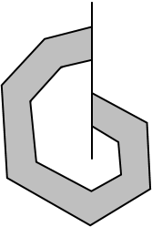
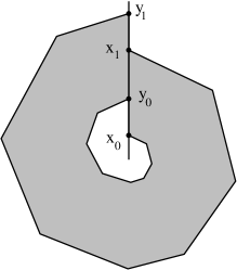
Figure 24. A G-region can form a single tube with disjoint ends (a simple G-tube) or the two ends can overlap (a spiral).

Lemma 8.2.

The length $L$ of a C-tube is at least twice its width $w$.

Proof.

The ends of a C-tube are disjoint intervals on the same $Q$-segment $S$, so the length of $S$ is at least $2w$. But both $P$-sides of the tube cover $S$ when projected orthogonally onto the line containing $S$, so both $P$-sides have length $\geq|S|\geq 2w$. The length of the tube is the minimum of these two path lengths, so is also $\geq 2w$. ∎

Lemma 8.3.

The length $L$ of a S-tube is at least twice its width $w$.

Proof.

Split the S-tube into four sub-tubes as follows. Each $P$-path in the tube is cut by a point where it crosses $S$ and this cuts the tube into two sub-tubes that also have width $w$, say $U_{1}$, $U_{2}$, which meet end-to-end. Each of these are split into two thinner tubes by the central $P$-path $\gamma_{1/2}$, giving four sub-tubes called $U_{1}^{i},U_{1}^{o},U_{2}^{i},U_{2}^{o}$, e.g., $U_{1}^{i}$ is the inner part of $U_{1}$ and its endpoints on $S$ separate the endpoints of the outer part $U_{1}^{o}$ on $S$. See Figure 25. Note that the length of the original S-tube is at least the minimum of the lengths of the two outer tubes (since they each have a $P$-boundary contained in the $P$-boundary of the S-tube).

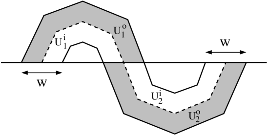
Figure 25. The outer tubes of a S-tube are shaded.

However, the endpoints of the outer $P$-boundary of an outer part are separated by at least distance $2w$, and each $P$-boundary of $S$ contains the outer $P$-boundary of one of its outer parts. Thus both $P$-boundaries have length at least $2w$. ∎

Lemma 8.4.

The length $L$ of a simple G-tube is at least its width.

Proof.

Suppose $I$ and $J$ are the ends of the spiral. If we project either $P$-side of the tube orthogonally onto $S$, then it covers either $I$ or $J$, so both sides of the tube are longer than the tube is wide. ∎

Putting together the last three lemmas we get

Corollary 8.5.

The length $L$ of a simple return tube is at least its width $w$. If the tube is not a $G$ tube, then $L\geq 2w$.

The more interesting and difficult return regions are the spirals: G-tubes where the $Q$-ends $[x_{0},x_{1}]$ and $[y_{0},y_{1}]$ overlap but are not identical.

Suppose $S$ is a spiral return tube and the corners are ordered on $S$ as $x_{0}<y_{0}<x_{1}<y_{1}$ and define $Q$-segments $I_{0}=[x_{0},y_{0}]$ and $I_{1}=[x_{1},y_{1}]$. See Figure 26. There is a $P$-path in that starts at $y_{0}$ and ends at a point $z$ in $I_{1}$ and is composed of $P$-paths in the tube joined end-to-end where they cross $S$.

If $z<y_{1}$, then we can remove the simple G-sub-tube with $Q$-end $[z,y_{1}]$ as shown in Figure 26 (the dark gray tube). What is left after removing this simple tube a pure spiral, a union of parallel $P$-paths that each consist of $N$ $P$-paths from the original tube. We call $N$ the winding number of the pure spiral (in this notation a simple tube has winding number one).

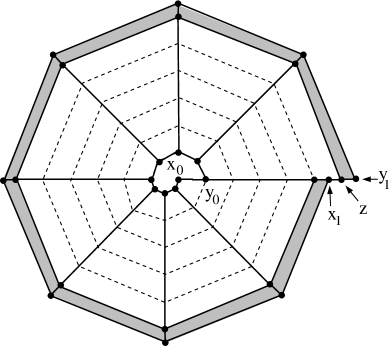
Figure 26. A spiral can always be divided into a simple tube (shaded) and a pure spiral. The pure spiral can be thought of as many parallel simple G-tubes that don’t cross $S$, or as one very long tube that crosses $S$ multiple times. The pure spiral here has five windings.

Since a pure spiral is made up of $N$ simple G-tubes all with the same width joined end-to-end, it is clear that the length of a spiral with $N$ windings should be at least $N$ times its width. However, we can do better than this, since each turn of the spiral is longer than the previous one.

Lemma 8.6.

A pure spiral with $N$ turns and width $w$ has length at least $N^{2}w$.

Proof.

Without loss of generality we may scale the spiral so the width $w=1$. Use the segment $[x_{0},y_{1}]$ to cut the entire spiral into $N$ simple G-tubes. The first has length at least $w$, because both $P$-boundaries project orthogonally onto one of the $Q$-ends. In general, both the parts of the $P$-boundary paths of the $j$th sub-tube have length at least $2j-1$. To see this, consider the curves in each half-plane defined by the line $L$ through $x_{0},y_{1}$, and project orthogonally onto $L$. The part in one half-plane projects to a segment of length at least $j-1$ and the other to a segment of length at least $j$. See Figure 27. Hence the $j$th tube has length at least $2j-1$. Summing $1+3+5+\dots+(2N-1)=N^{2}$ gives the result. ∎

Figure 27. Estimating the length of a G-curve.

The argument proving Lemma 8.6 will be used again in Section 18. Next we slightly refine Lemma 8.1

Lemma 8.7.

Suppose $n$ is the number of isosceles pieces in an isosceles dissection. Every $P$-path $\gamma$ with $3n+1$ segments contains a sub-path that begins and ends on the $Q$-end of a chain and is a return path of one of the four types described above (S, C, G1, G2).

Proof.

Apply Lemma 8.1 to the initial path of $2n+1$ steps, to get a return path of one of the four types. If the path already begins and ends on the $Q$-end of a chain there is nothing to do. If it begins and ends at an interior $Q$-segment of the chain then by deleting or extending the paths as shown in Figure 28 we can obtain a path that begins and ends on the $Q$-end of the chain. The number of steps added is less than $n$, so the new path must be a sub-path of $\gamma$. ∎

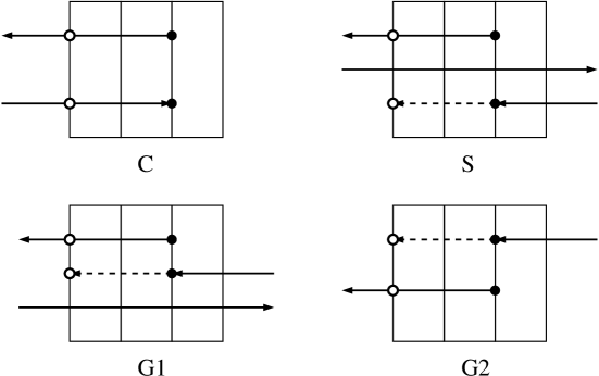
Figure 28. A return path ending inside a chain can easily be modified to start and finish on the $Q$-end of the chain (the extensions are shown as dashed lines and follow $P$-paths). Black dots are the original endpoints of the path an the white dots are the modified endpoints.

We say that a return region is standard if is of one of the types (C, S, G1, G2) discussed above and if it begins and ends on segments that are the $Q$-ends of some chains (possibly the same chain or two different chains). The following is one of the key estimates of this paper.

Lemma 8.8.

If $\Omega$ has an isosceles dissection into $n$ pieces with $M$ chains, then there are $O(M)$ standard return regions with disjoint interiors so that any $P$-path with more than $5n+1$ segments must hit one of the regions.

Proof.

Each chain in the dissection has two $P$-boundaries. Each of these $P$-boundaries may or may not be part of the $P$-boundary of a standard return region. If it is, then associate to the $P$-boundary of the chain the maximal width standard return region that contains the $P$-boundary of the chain in its own boundary. Note that at most $2M$ return regions can be selected in this way, since there are $M$ chains and each has two $P$-boundaries.

We claim that any $P$-path $\gamma$ in the dissection with $5n+1$ steps contains a sub-path that crosses one of the selected return regions. Let $\gamma^{\prime}$ be the path obtained by deleting $n$ steps from each end of $\gamma$. By Lemma 8.7, $\gamma^{\prime}$ contains a sub-path $\gamma^{\prime\prime}$ that is a return path of one of the four standard types and which begins and terminates on the $Q$-end of a chain. Thus the set of paths parallel to $\gamma^{\prime\prime}$ forms a standard return tube $T$ of maximal width. If $T$ is one of the chosen return regions, then we are done since $\gamma^{\prime\prime}\subset\gamma$ crosses $T$.

On the other hand, suppose $T$ is not one of the chosen regions. Since $T$ is maximal, it contains the $P$-boundary of some chain $C$ within its own $P$-boundary. Since $T$ was not chosen, there must be another return region $T^{\prime}$, at least as wide as $T$, that was chosen and $T\cap C\subset T^{\prime}\cap C$. Thus every path crossing $T$ hits $T^{\prime}$. Thus $\gamma^{\prime\prime}$ hits $T^{\prime}$. If we add $n$ steps to both ends of $\gamma^{\prime\prime}$, the new, longer path must now cross $T^{\prime}$, but it is still a sub-path of $\gamma$. Thus $\gamma$ crosses some return region in the chosen collection. This proves the claim.

The collection of maximal width return regions defined above may overlap. To get disjointness, we order the chosen regions $R_{1},\dots,R_{m}$, $m=O(M)$, from widest to narrowest and label the first region “protected” and label the remainder “unprotected”. At each stage we look at the first unprotected region $R_{k}$ in the current list and see if there are any $P$-paths strictly crossing it that intersect a protected region (anything earlier in the list). If there is no such path, then label $R_{k}$ protected, and move to the next region.

If there is a $P$-path $\gamma$ strictly crossing $R_{k}$ that hits a protected region $R_{j}$, then remove from $R_{k}$ any $P$-paths that hit $R_{j}$. Since $R_{j}$ is at least as wide as $R_{k}$, removing these paths gives a connected return region $R_{k}^{\prime}\subset R_{k}$ (possibly empty). Now re-sort the list by width. $R_{k}^{\prime}$ either stays where it is or moves later in the list; the protected regions all stay where they are. Since two regions will never overlap after the first time they were compared, this process stops after at most $m^{2}$ steps, and gives a collection of return regions with disjoint interiors. Moreover, once a region is protected, it is never modified again and is part of the final collection.

Finally, we have check that every long enough $P$-path hits one of the disjoint regions. If $\gamma$ is any path with $5n+1$ segments then it crossed some region in the original list. Suppose $R_{\gamma}$ is the first region on the original sorted list that is crossed by $\gamma$. If a part of $R_{\gamma}$ containing $\gamma$ is deleted in the construction, then $\gamma$ must hit a protected return region. Thus $\gamma$ hits a return region in the final collection, as desired. ∎

This lemma is used in the proofs of both Theorems 1.1 and 1.3. In both cases we will reduce to meshing a region $\Omega$ that has an isosceles dissection. We will propagate the non-conforming vertices until they either hit the boundary of $\Omega$ or hit the $Q$-end of a return region. By Lemma 8.8, one of these two options must occur with $O(n)$ steps. The proofs of the two theorems differ mostly in how we construct $\Omega$ and how we mesh inside the return regions.

9. Proof of Theorem 1.3: reduction to a meshing lemma

This is the first of four sections that construct the almost nonobtuse triangulation in Theorem 1.3. Unlike the proofs of Theorems 1.1 and 1.2, the proof of Theorem 1.3 does not make use of Theorem 2.1 to create the triangulation; we shall construct the triangulation directly. However, we will use the result of Bern, Mitchell and Ruppert [9] that any simply $n$-gon has a nonobtuse triangulation with $O(n)$ triangles. We will also make use of return regions and bending paths, both ideas we shall use again in the proof of Theorem 1.1.

As in the proof of Theorem 1.2, we start with a PSLG that is a triangulation. In that earlier proof we divided each triangle $T$ into a central triangle and three isosceles triangles. Here we will replace the single central triangle by a simple polygon that approximates a triangle with circular edges.

Given a triangle $T$ with vertices $v_{1},v_{2},v_{3}$, let $C$ be the inscribed circle and let $z_{1},z_{2},z_{3}$ be the three points where this circle is tangent to the triangle (numbered so that $z_{k}$ lies on the side of $T$ opposite $v_{k}$). Any pair of the $z$’s are equidistant from one of the vertices of $T$ and hence are connected by a circular arc centered at this vertex. This defines a central region bounded by three circular arcs, each pair of arcs tangent where they meet (see the shaded area on the left of Figure 29). We will replace each of these circular arcs by a polygonal path inscribed in the arc. For example, let $\gamma_{1}$ be a polygonal arc inscribed in the circular arc connecting $z_{2}$ and $z_{3}$. If $\gamma_{1}$ consists of $m$ equal length segments, then the angle subtended from $v_{1}$ by these segments is less than $\pi/m$, (since $\gamma_{1}$ subtends at most angle $\pi$). If we then connect the vertices of $\gamma_{1}$ to $v_{1}$ we obtain a chain of isosceles triangles all with angle $\leq\theta=\pi/m$. See the right side of Figure 29. Taking the union of these isosceles triangles over all $T$ in the original triangulation gives the region $\Omega$, that clearly has a $\theta$-nice isosceles dissection with $O(n)$ chains and $O(n/\theta)$ pieces.

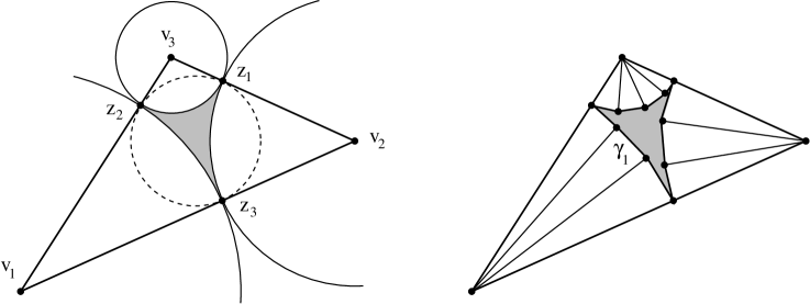
Figure 29. We define a simple polygon by inscribing polygon arcs on circular arcs as shown above. If we use $m$ evenly points on each arc then remaining region clearly has a $\theta$-isosceles dissection for $\theta=\pi/m$.

Lemma 9.1.

Suppose $\Omega$ is a region that has a $\theta$-nice isosceles dissection (both triangles and quadrilaterals are allowed). Assume that the dissection has $O(n)$ chains and $O(n/\theta)$ pieces. Then there is a mesh of $\Omega$ using $O(n^{2}/\theta^{2})$ $\theta$-nice quadrilaterals and triangles. Moreover, each dissection piece $T$ contains at most $O(n/\theta)$ mesh elements and every mesh element $Q$ contained in $T$ is bounded by at most two sub-segments of the $Q$-sides of $T$ (possibly points) and at most two $\theta$-paths in $T$ (possibly the vertex of $T$, if $T$ is a triangle).

We will prove this in the next three sections. We can deduce Theorem 1.3 from Lemma 9.1 as follows. By a result of Bern, Mitchell and Ruppert, each central polygon has a nonobtuse triangulation with at most $O(1/\theta)$ triangles. This triangulation may place extra vertices on the edges of the central polygon, but not more than $O(1/\theta)$ vertices in total. Each such edge $e$ is the base of one of the isosceles triangles $T$ in the dissection, and we connect the extra vertex on $e$ to the opposite vertex of $T$ by a $Q$-segment $S$. See Figure 30.

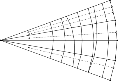
Figure 30. Each isosceles triangles $T$ in the dissection of $\Omega$ is meshed by at most $O(n/\theta)$ quadrilaterals and triangles (here a chain of four triangles is shown). Connecting “extra” vertices (white dots) on the base of $T$ to the opposite vertex thus creates at most $O(n/\theta)$ extra mesh pieces per dissection triangle.

This creates a new $\theta$-nice quadrilateral or triangle for each $\theta$-path that $S$ crosses. Since there are at most $O(n/\theta)$ such paths per piece, each extra vertex on $e$ creates at most $O(n/\theta)$ new elements of the mesh. Since there are $O(n)$ central polygons and each has at most $O(1/\theta)$ extra boundary points coming from its nonobtuse triangulation, at most $O(n^{2}/\theta^{2})$ extra pieces are created overall.

As the final step, we add diagonals to the quadrilateral pieces of the mesh, getting a triangulation. Since all the quadrilaterals are $\theta$-nice, the resulting triangles have maximum angle $90^{\circ}+\theta$, which proves Theorem 1.3.

Our application of Lemma 9.1 to Theorem 1.3 only needs to apply to dissections consisting entirely of triangles, but has been stated for more general isosceles dissections which may use both triangles and quadrilaterals. The extra generality does not lengthen the proof at all, but it is useful for the application to optimal quad-meshing given in [11]. That application involves an isosceles dissection that uses only trapezoid pieces; the precise variant of Lemma 9.1 that is needed in that paper will be stated and proved in Section 13.

10. Proof of Lemma 9.1: outside the return regions

We continue with the proof of Theorem 1.3, by starting the proof of Lemma 9.1. In this section we will mesh the part of $\Omega$ that is outside the return regions.

Let $\{R_{k}\}_{1}^{N}$ be the disjoint return regions for $\Omega$ given by Lemma 8.8. Since there are $O(n)$ chains there are $O(n)$ return regions. For each triangle $T_{k}$, and each of the three vertices of $T_{k}^{\prime}$ on its boundary, construct the $P$-path starting at this point and continued until it hits another cusp point, leaves $\Omega$ or enters a return region. Lemma 5.2 says these paths cut the isosceles pieces of the dissection into isosceles pieces that form a mesh. By Lemma 8.8, each $P$-path we generate terminates within $O(n/\theta)$ steps and there are less than $3n$ of these paths (at most three per triangle), so a total of $O(n^{2}/\theta)$ mesh pieces are created outside the return regions. Moreover, each such path crosses a single dissection piece at most $O(1)$ times. Thus each dissection piece can be crossed at most $O(n)$ times but such paths.

Next we place $O(1/\theta)$ evenly spaced points on both $Q$-sides of each return region (the reason for this will be explained in the next section). Each of these points is propagated by $P$-paths outside the return region it belongs to, until it runs into the boundary of $\Omega$ or hits the $Q$-side of some return region (possibly the same one they started from). As above, this generates a $\theta$-nice mesh outside the return regions. There are $O(n)$ return regions and $O(1/\theta)$ points per region to be propagated. Each path continues for at most $O(n/\theta)$ steps, so at most $O(n^{2}/\theta^{2})$ mesh elements are created in total. Moreover, each dissection piece is crossed at most $O(1)$ times by each path, so is crossed $O(n/\theta)$ times in total by such paths.

11. Proof of Lemma 9.1: the simple tubes

Next, we have mesh inside the return regions. In this section, we deal with the return regions that are simple tubes and in the next section we deal with spirals.

For the first time we will use $\theta$-paths rather than $P$-paths (recall that a $\theta$-path is made up of segments that are within $\theta$ of parallel to the base of the isosceles piece; when we cut a $\theta$-nice piece by a $\theta$-path we get two $2\theta$-nice pieces). We need the following lemma.

Lemma 11.1.

Suppose $Q$ is a tube whose width $w$ is at most $\sin\theta$ times its minimal-length $\tilde{\ell}$. Then opposite corners of $Q$ can be connected by a $\theta$-path inside the tube.

Proof.

Suppose $T$ is a $\theta$-nice isosceles piece and $x,y$ are the endpoints of a $P$-segment $S=[x,y]$ crossing $T$. Then any point $z$ on the same side as $y$ and within distance $\sin(\theta)|x-y|$ can joined to $x$ by a $\theta$-path. See Figure 31. Thus if $\{T_{k}\}$ is an enumeration of the pieces making up the tube and $\ell_{k}$ is the minimal base length of the $k$th piece, then we can create a $\theta$-path that crosses the tube and whose endpoints are displaced by $\sum_{k}\ell_{k}\sin\theta=\tilde{\ell}\sin\theta$ with respect to a $P$-path. This proves the lemma. ∎

Figure 31. Clearly $|p-y|\geq|q-y|=|x-y|\sin\theta\geq\tilde{\ell}\sin\theta$ where $q$ is the closest point to $y$ on the line making angle $\theta$ with the segment $xy$.

Corollary 11.2.

If $R$ is return region that is a C-tube, S-tube or simple G-tube, then we can cut $R$ into $O(1/\theta)$ parallel sub-tubes and connect opposite corners of the each tube by a $\theta$-path contained in that tube.

Proof.

Suppose the return region $R$ has length $L$ and width $w$. Choose an even integer $M\geq{4}/{\sin\theta}$ and split the return region $R$ into the disjoint union of $M$ thinner tubes $\{T_{j}\}$ of width $w/M$. By Lemmas 8.2, 8.3 and 8.4 each of these new tubes has length that is at least $w$ and width equal to $w/M$. Thus each has length that is at least $M$ times as long as its width.

Since $M\geq 2$, each of our thin tubes is half of a thicker tube that is still inside the given tube $R$. By Lemma 7.1

$$\tilde{\ell}(T_{j})\geq\frac{1}{4}\ell(T_{j})\geq\frac{1}{4}\ell(R)\geq\frac{1}{4}w.$$

On the other hand, the width of $T_{j}$ is $w/M$. Hence the minimal-length of each tube $T_{j}$ is more than $M/4=1/\sin\theta$ times its width, so the previous Lemma 11.1 applies to $T_{j}$, as desired. ∎

We can now continue with the proof of Lemma 9.1. We then cut the return region into $O(1/\theta)$ parallel tubes as described above, and divide each tube by a $\theta$-path connecting opposite corners. This meshes each tube using $2\theta$-nice pieces. Any $P$-path hitting a $Q$-end of one of these tubes is then propagated to a corner on the opposite end of the tube by standard quadrilateral propagation paths. This gives a $2\theta$-nice mesh of the tube that is consistent with all the meshes created outside the tube.

Since there were at most $O(n/\theta)$ $P$-paths that might terminate and each return region has at most $O(n/\theta)$ isosceles pieces, at most $O(n^{2}/\theta^{2})$ $2\theta$-nice triangles and quadrilaterals are created inside all the return regions. Moreover, each dissection piece is crossed by at most $O(n/\theta)$ paths (there are $O(1/\theta)$ paths per return region and $O(n)$ return regions), so it contains at most this many mesh pieces.

12. Proof of Lemma 9.1: the spirals

This is the final section in the proof of Theorem 1.3. Here we prove Lemma 9.1 inside the spiral return regions.

Since any spiral can be divided into a simple G-tube and a pure spiral, and we can treat the simple tube as above, it suffices to deal with the pure spirals. Let $N$ be the winding number of the spiral; we may assume $N\geq 2$, since otherwise the spiral can be treated as a tube and can be triangulated as in the previous section. Let $p$ be the number of isosceles pieces that are hit by the spiral (this is the number of steps it take to complete one winding of the spiral).

The spiral can be divided into $N$ tubes joined end-to-end, each starting and ending on the same $Q$-edge of some isosceles pieces. We divide the first and last of these tubes into $O(1/\theta)$ parallel thin tubes. Then any $P$-path that enters the tube from either end can be $\theta$-bent so that it terminates at the corner of one of the thin tubes after winding once around the spiral.

If $N=O(1/\theta)$, then we simply propagate all the interior corners of the thin tubes at one end of the spiral around the spiral until they run into the corners of the thin tubes at the other end. This generates $O(N\cdot p\cdot\theta^{-1})=(p\theta^{-2})$ new vertices. See Figure 32.

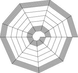
Figure 32. Cut the inner and outer tubes into $O(1/\theta)$ parallel narrow tubes and $\theta$-bend all entering $P$-paths so they terminate inside these narrow tubes. The corners of the narrow inner tubes are then propagated around the $N$ turns of the spiral until they hit the corners of the narrow outer tubes. This creates a $2\theta$-nice mesh of the spiral using $O(nN/\theta)$ pieces. The figure shows $p=9$ and $N=6$.

If $N\gtrsim 2\theta^{-1}\geq 1/\sin(\theta)$ then after $O(\theta^{-1})$ spirals, we can create a $\theta$ curve that is a closed loop and we let the paths generated by the interior corners of the inner thin part hit this closed loop. We create another $\theta$-bent closed loop at radius $N-2$ and let the paths generated by the corners of the outer thin tubes hit this. No propagation paths enter the region between the two closed loops and a total of $O(p\theta^{-2})$ vertices are used. See Figure 33.

       

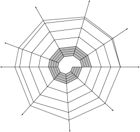
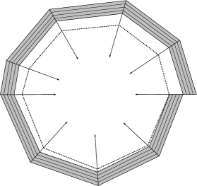
Figure 33. If the winding number is much larger than $\frac{1}{\theta}$, then after $O(1/\theta)$ windings we can create a closed $\theta$-bent loop (the dashed curve). We then propagate the corners of the narrow inner tunes until they hit a vertex of this closed loop. We can also create a $\theta$-bent loop one winding in from the outer tube and use it similarly to propagate the corners of the narrow outer tubes until they hit a vertex of this loop.

The propagation paths cut the spiral into $2\theta$-nice triangles and quadrilaterals. Moreover, as in the case of simple tubes, it is easy to check that each dissection piece is crossed by at most $1/\theta$ paths in the construction of each spiral. Since there are $O(n)$ spirals, this means there are at most $O(n/\theta)$ such crossings of a dissection piece in total. The propagation paths that enter each spiral cross each dissection piece at most once, and there are $O(n/\theta)$ such paths in total, hence $O(n/\theta)$ such crossings of each piece.

This completes the proof of Lemma 9.1, and hence the proof of Theorem 1.3.

13. A lemma for quadrilateral meshing

We now restate our conclusions in a form that is useful for proving the theorem on optimal quad-meshing in [11]. Readers interested only in Theorem 1.1 may skip this section.

Theorem 13.1.

Suppose that $W$ is a polygonal domain with an isosceles trapezoid dissection with $n$ pieces. Suppose also that $0^{\circ}\leq\theta\leq 15^{\circ}$ and that every dissection piece is $\theta$-nice. Finally, suppose the number of chains in the dissection is $M$. Then we can remove $O(M/\theta)$ $\theta$-nice quadrilaterals of uniformly bounded eccentricity from $W$ so that the remaining region $W^{\prime}$ has a $2\theta$-nice quadrilateral mesh with $O(nM/\theta)$ elements. At most $O(M/\theta)$ new vertices are created on the $Q$-boundary of $W^{\prime}$. At most $O(M)$ vertices are created on the $P$-boundary of $W^{\prime}$, and no more than $O(1)$ vertices are placed in any single $P$-side of any dissection piece of $W^{\prime}$. For this quad-mesh, any boundary point on a $Q$-side of $W^{\prime}$ propagates to another boundary point after crossing at most $O(n)$ quadrilaterals.

Proof.

The proof is exactly the same as the argument of the last few sections, except for some slight modifications inside the return regions.

For each return region we place $O(1/\theta)$ equally space points along the two $Q$-sides of the region and propagate these outside the return regions until they hit the boundary of $\Omega$ or hit the $Q$-side of some return region. There are $O(M/\theta)$ such paths and they generate at most $O(Mn/\theta)$ quadrilaterals and $O(M/\theta)$ endpoints on $Q$-sides of $\partial\Omega$.

First consider return regions that are simple tubes. As before, split each such region into $O(1/\theta)$ parallel sub-tubes and so that in each sub-tube we can connect opposite corners by a $\theta$-path. Now, however, we remove a small quadrilaterals at a pair of opposite corners of the tube. These quadrilaterals have one edge on a $P$-boundary of the tube, one edge on a $Q$-end of the tube, one vertex in the interior of the tube and the two edges adjacent to this vertex are chosen to lie a $P$-segment and a $Q$-segment. See Figure 34.

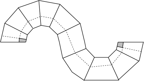
Figure 34. We place quadrilaterals (shaded) at opposite corners of a tube, and connect the internal corners by a $\theta$-path. Every path entering tube either immediately hits the shaded quadrilateral at that end, or propagates to hit the shaded quadrilateral at the other end. We also have to propagate the interior corner of the shaded quadrilateral along a $Q$-path. This gives a mesh of every tube by $2\theta$-nice quadrilaterals.

We then connect the interior corner of each of the two quadrilaterals by a $\theta$-curve. This requires less displacement than connecting the corners, so it is clearly possible to do this (to make it easier to see, we could always increase the number of tubes and decrease their width by a fixed factor). We have freedom in choosing the size of the quadrilaterals, and so we can arrange for all the quadrilaterals chosen in the same dissection trapezoid to have sides along the same $Q$-segment. Thus when we $Q$-propagate the corners of the quadrilaterals, only two extra points will be created on the $P$-side of the dissection piece containing such a quadrilateral.

If we apply quadrilateral propagation to each $P$-path entering the tube from either end, it crosses the tube and hits a $Q$-side of the removed quadrilateral at the other end of the tube. See Figure 34. This gives a $2\theta$-nice quadrilateral mesh inside the modified tubes.

Inside the spirals we do a similar thing. In the previous proof, paths inside spirals were terminated by bending them in a sub-tube of the spiral until they hit a corner on the opposite side of the tube from where they entered, in order to form a loop. so the same construction works. Outside the return regions, the $P$-paths convert the $\theta$-nice dissection into a $\theta$-nice quadrilatal mesh (previously the only triangles created by the $P$-paths were in triangular pieces of the dissection, which we now assume don’t exist). See Figures 35 and 36. ∎

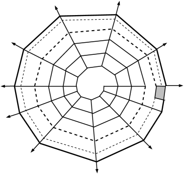
Figure 35. For spirals with $\gg\theta^{-1}$ windings, we can make a $\theta$-path loop in the $j$th spiral when $j\gtrsim 1/\theta$ (solid thick curve). Then place a quadrilateral as shown with one edge on the loop; one corner is $\theta$-propagated around the spiral once to hit the center of a side of the same quadrilateral (thin dashed curve). The boundary of the spiral is $\theta$-bent to hit the other corner (thick dashed curve).

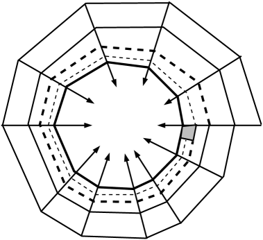
Figure 36. The quadrilateral construction near the outside of a large spiral. This is similar to the construction in Figure 35, but we can do it in the sub-tube adjacent to the outermost one. The two constructions give a $2\theta$-nice mesh of the entire spiral (minus the two quadrilaterals).

14. Overview of the proof of Theorem 1.1

The remainder of the paper gives the proof of Theorem 1.1. In this section we give the overall strategy of the proof and we will provide the details in the following sections.

The proof combines ideas already seen in the proofs of Theorems 1.2 and 1.3 but requires a different displacement estimate in tubes and a more intricate construction in the spirals. As explained in Section 2, it suffices to prove Theorem 2.3: assume $\Gamma$ is a triangulation and show we can place $O(n^{2.5})$ points along the edges so that each triangle becomes Gabriel. As in the proof of Theorem 1.2 we start taking the dissected domain $\Omega$ to be the original triangles $\{T_{k}\}$ with the central triangles $\{T_{k}^{\prime}\}$ removed (recall the vertices of $T_{k}$ are the three points where the inscribed circle touches the triangle $T_{k}$). We do not use the “approximate circular-arc triangles” that were used in the proof of Theorem 1.3.

For each triangle $T_{k}$, remove the closed triangle $T_{k}^{\prime}$ as in Section 4. As before, $T_{k}\setminus T_{k}^{\prime}$ is a union of three isosceles triangles. Keep the isosceles triangles with angle $<90^{\circ}$; as explained at the end of Section 4, isosceles triangles with angles $\geq 90^{\circ}$ can be ignored because adding any set of points to the $Q$-edges will make the triangle Gabriel. The remaining region $\Omega$ thus has an isosceles dissection by $O(n)$ acute triangles. We construct return regions for $\Omega$ just as before.

Each vertex of each $T_{k}^{\prime}$ are propagated by $P$-paths until then leave $\Omega$ or hit the $Q$-side of a return region. This creates $O(n^{2})$ crossing points on $\Gamma$.

If a return region has $k$ isosceles pieces then we will place $O(\sqrt{k})$ even spaced points in each $Q$-end of the region and propagate these until they leave $\Omega$ or hit a return region. Since $k=O(n)$, this creates at most $O(n^{2.5})$ new points. If different return regions had to use distinct isosceles pieces this estimate would be $O(n^{2})$ instead. Improving the exponent in Theorem 1.1 seems to be entirely a matter of understanding the behavior of distinct return regions that share isosceles pieces.

Why do we split the $Q$-ends of the return regions into $O(\sqrt{k})$ pieces? When we bend the $P$-paths inside the return regions, we must verify that the Gabriel condition is satisfied by the points that we generate. This is a more restrictive condition than the $\theta$-bending of the earlier proof, so paths can be bent less and hence take a more steps to terminate. The difference is illustrated in Figure 37. The left side shows the range of options for a $\theta$-segment crossing a single rectangle; the allowable displacement is roughly $\theta|a-b|$. The center and right pictures of Figure 37 show the restrictions on a Gabriel path. Note that there are two such restrictions: the exit point $b$ must be between the Gabriel disks tangent at $a$ and the entrance point $a$ must be between the disks tangent at $b$. This restricts $b$ to an interval of length approximately $|a-b|^{2}/w$, where $w$ is the width of the piece. This estimate will be made more precise in the next section; the main point is that it shrinks quadratically with $|a-b|$ whereas the estimate for $\theta$-paths decreased linearly. Thus the proof of Theorem 1.1 requires longer, narrower tubes than the proof of Theorem 1.3.

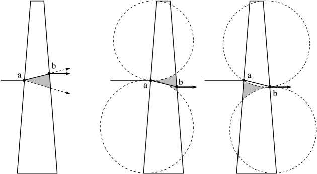
Figure 37. A $\theta$-bent path can reach any point defined by a cone with angle $2\theta$, but a Gabriel bent path can only reach points defined by the cusp between two tangent disks. Moreover, this is a two part condition: the exit point must be the cusp defined by the entrance point and the entrance point must be in the cusp defined by the exit point.

To illustrate the idea, consider a simple case: a square divided into $k$ thin parallel rectangles. See Figure 38. A Gabriel path crossing the square takes $k$ steps, each with displacement $\simeq 1/k^{2}$, so the total displacement is $\simeq 1/k$. At first glance, this seems to say we should cut the square into $O(k)$ parallel tubes; then we could get all entering paths to terminate before hitting the far side of tube. This works, but leads to the estimate $O(n^{3})$ in Theorem 1.1.

Figure 38. A Gabriel-bent path must stay outside certain pairs of tangent disks. When we cut a unit square into $\frac{1}{k}\times 1$ rectangles then a Gabriel path has total displacement at most $O(1/k)$. If we cut the square into $O(\sqrt{k})$ horizontal tubes, paths in each tube take $k$ steps with displacement of $k^{-3/2}$ and hence total displacement of $1/\sqrt{k}$. Since this is also the width of the tube, we can Gabriel-bend a path to hit the side of a tube before leaving it.

We can do better. Cut the square into $\sqrt{k}$ tubes instead. Now the tangent disks have diameter $k^{-1/2}$ and the cusp regions where we choose our next point have height $\simeq\frac{1}{\sqrt{k}}(\frac{1}{\sqrt{k}}/\frac{1}{k})^{2}=k^{-3/2}$. Thus a Gabriel path takes $k$ steps, each with displacement $\simeq k^{-3/2}$, for a total displacement $\simeq k^{-1/2}$, which is the approximate width of the tube. Thus using only $O(\sqrt{k})$ tubes, we can bend Gabriel paths enough to hit the far corner of the tube (and thus terminate).

We shall prove in the next two sections this holds for any return regions that are simple tubes, not just squares with rectangular pieces. Each return region that is a C-tube, S-tube or simple G-tube will be split into $O(\sqrt{k})$ narrow parallel tubes and the entering propagation paths will be Gabriel bent until they a far corner of the tube; here $k$ is the number of isosceles pieces forming the tube.

We also place $O(\sqrt{k})$ narrow parallel sub-tubes at the two ends of spiral return regions, i.e., we subdivide the innermost and outermost windings of the spiral. As with simple tubes, all paths entering the spiral can be bent within these narrow tubes to terminate within $O(k)$ steps. But then we have to propagate both the external and internal corners of the narrow tubes. The external corners propagate outside the spiral until they terminate just as described for the corners for narrow tubes in the previous paragraph.

The most difficult part of the proof of Theorem 1.1 is dealing with the $\sqrt{k}$ internal corners that propagate through the spiral; since we have no bound for the number $N$ of windings of the spiral in terms of $n$, this could produce arbitrarily many new vertices. Thus propagation paths of the internal corners must be bent to terminate earlier. Consider the case of paths that start near the inner end of the spiral (the outer part is handled in the same way, but is easier, since the windings of the spiral are longer). We consider what happens for very large spirals (where the number of windings $N$ is bigger than the number $k$ of isosceles pieces in the spiral; for smaller values of $N$ we truncate the construction at the appropriate stage.)

We first bend the propagation paths so that adjacent paths merge, and then merge adjacent merged paths, and continue until all the propagation paths generated by the $O(\sqrt{k})$ internal corners have merged into a single path. This occurs around winding $k^{1/3}$. This path is then propagated as a $P$-path out to winding $k^{1/2}$. See Figure 39.

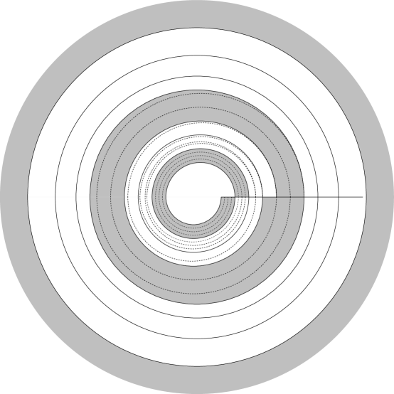
Figure 39. This illustrates the stages in the spiral construction. First (light gray), we divide the tube into thinner tubes and entering paths are bent to hit the sides of these. Next (white), the thin tubes are bent and collapsed in pairs; in this figure four tubes are merged into one after two windings. In the third stage (gray), the single tube is propagated until we can bend it to intersect itself. Next (white) comes a sequence of closed loops that gradually grow further apart. Finally we reach the empty region (gray), where no paths propagate. This figure gives a rough idea of the construction, but scales have been drastically compressed to make all the stages visible in the same picture.

At this stage we have enough freedom to bend the curve to hit itself, forming a closed loop that wraps once around the spiral. This is similar to what we did in the proof of Theorem 1.3, but in this case, in order for this closed loop to be Gabriel, there must be another (larger) closed loop parallel to it. This did not occur in Theorem 1.3. This constraint requires us to construct a sequence of parallel closed loops in the spiral between windings $k^{1/2}$ and $k$. The closed loops gradually can become farther and farther apart; only $O(\sqrt{k})$ loops are used in all. At winding $k$, there is no need for a “next” loop and the sequence of closed loops ends. The part of the spiral beyond winding $k$ is an “empty” region until we reach a closed loop coming from the analogous construction in the outer half of the spiral.

In the remainder of the paper we give the details of the argument sketched above.

15. Gabriel bending in isosceles pieces

This section contains the main estimate used in proof of Theorem 1.1.

Suppose $a$ and $b$ are endpoints of a $P$-path in an isosceles piece $T$. If we keep $a$ fixed, how far we can move $b$ and still have the Gabriel condition hold? More precisely, can we find an $\epsilon>0$ so that all points on the same $Q$-side as $b$ that are within distance $\epsilon$ of $b$ can be connected to $a$ by a Gabriel segment? If this holds we say that the allowable displacement for the piece is at least $\epsilon$.

Lemma 15.1.

Suppose $T$ is an isosceles piece of width $w$. Suppose $[a,b]$ is a $P$-segment crossing $T$ and $R$ is the distance of $a$ from the vertex of the piece ($R=\infty$ if the piece is a rectangle). Then if $c$ is a point on the same $Q$-side as $b$ and is within distance

(15.1) $$\epsilon=\frac{|a-b|^{2}}{4}\max(\frac{1}{w},\frac{1}{R}),$$

of $b$, then $[a,c]$ is a Gabriel segment crossing $T$. In particular, the allowable displacement is at least $\epsilon$.

Proof.

First suppose the isosceles piece is a rectangle ($R=\infty$). Consider disjoint sub-segments of the $Q$-side containing $a$ that have $a$ as a common endpoint and consider the disks $D_{1},D_{2}$ with these segments as diameters. See Figure 40. Assume these disks have radii $r$ and $s$. The diameters of these disks are disjoint segments that both lie on the same non-base side of an isosceles piece, so their length adds up to be less than the width of the piece, i.e., $2r+2s\leq w$. Thus $\max(2r,2s)\leq w$.

Figure 40. The segment $[a,b]$ is a $P$-segment for a rectangular piece. A simple estimate shows $|c-b|\geq|a-b|^{2}/r$ and $|d-b|\geq|a-b|^{2}/s$.

Suppose $[c,d]$ is the $Q$-segment containing $b$ that is disjoint from these disks (again, see Figure 40). We want to estimate $|c-b|$ and $|d-b|$ from below. Such a lower bound gives the desired lower bound on the allowable displacement.

If the disk $D_{1}$ is too small, i.e., $r<|a-b|$, then the disk $D_{1}$ does not hit the $Q$-side containing $b$ and the Gabriel condition is automatically satisfied. Thus we may assume $r\geq|a-b|$. Then by the Pythagorean theorem

$$|c-b|=r-\sqrt{r^{2}-|a-b|^{2}},$$

or (using $1-\sqrt{1-y}\geq y/2$ on $[0,1]$),

$$\frac{1}{r}|c-b|=1-\sqrt{1-\frac{|a-b|^{2}}{r^{2}}}\geq\frac{|a-b|^{2}}{2r^{2}}$$

so $|c-b|\geq|a-b|^{2}/2r$. The calculation for the other disk is identical, so the two disks omit all points within distance

$$\epsilon=|a-b|^{2}\min(\frac{1}{r},\frac{1}{s})\geq\frac{|a-b|^{2}}{2w}.$$

of $b$. Since $1/R=0$ in this case, this implies (15.1).

Next we consider what happens when the piece is not a rectangle. To be concrete, we assume one $Q$-side lies on the real axis, the vertex of the piece is at $-R$ and the $P$-path connects $a=0$ to $b$ in the upper half-plane. Suppose the piece has angle $\theta$. Some elementary trigonometry shows that the disk $D_{1}$ does not hit the $Q$-side containing $b$ if (see Figure 41)

$$r<(R-r)\sin\theta.$$

Figure 41. If $r,s$ are small enough then the Gabriel disks for one $Q$-side don’t hit the other $Q$-side.

Since $|a-b|=2R\sin\theta/2$, this is equivalent to

(15.2) $$r<R\frac{\sin\theta}{1+\sin\theta}=\frac{|a-b|\sin\theta}{2\sin(\theta/2)(1+\sin\theta)}.$$

By the double angle formula, for $0\leq\theta\leq\pi/2$ we have $\sin\theta=2\sin\frac{\theta}{2}\cos\frac{\theta}{2}$, so

(15.3) $$\frac{\sin\theta}{2\sin(\theta/2)(1+\sin\theta)}=\frac{\cos\theta/2}{(1+\sin\theta)}\geq\frac{\cos\pi/4}{(1+\sin\pi/2)}=\frac{1}{2\sqrt{2}}.$$

Hence (15.2) holds if $r<|a-b|/2\sqrt{2}$. If this condition holds, then the point $c$ is a corner of the piece $T$, so the estimate holds trivially to the left of $b$. Therefore we may assume $r\geq|a-b|/2\sqrt{2}$ in what follows. Note also that this implies $w\geq|a-b|/\sqrt{2}$ since $r\leq w/2$.

A similar calculation shows $D_{2}$ does not hit the opposite $Q$-side if

$$s<\frac{|a-b|\sin\theta}{\sin(\theta/2)(1-\sin\theta)}=2|a-b|\frac{\cos\theta/2}{1-\sin\theta}.$$

See Figure 41. The trigonometric function on the far right is increasing for $\theta\in[0,\pi/2]$ (compute the derivative), so it takes its minimum value $1$ at $\theta=0$. Hence $D_{2}$ does not hit the opposite $Q$-side if $s<2|a-b|$. In this case $d$ is a corner of the isosceles piece and the lemma holds trivially to the right of $b$. Therefore we may assume $s\geq|a-b|$ in what follows.

Now suppose we have an isosceles piece with angle $\theta>0$. We normalize the picture as in Figure 42 with one $Q$-side along the real axis, the vertex of the piece at $-R$. The other $Q$-side is labeled $L$. We consider a $P$-path with one endpoint at the origin and the other endpoint (labeled $b$ in the figure) on $L$ in the upper half-plane. We also consider disks $D_{0}$, $D_{1}$, $D_{2}$ centered at points $-R$,$-r$, $s$ on the real line that are tangent at the origin. We let $[c,d]$ be the segment of $L\setminus(D_{1}\cup D_{2})$ that contains $b$. See Figure 42.

Figure 42. We want a lower bound on $|b-c|$ and $|b-d|$ in terms of $|a-b|$, $r$, $s$ and $R$. We prove this by applying the transformation $z\to 1/z$ to this picture, to get the picture in Figure 43.

Figure 43. This is the inversion of Figure 42. The point $a=0$ maps to $a^{\prime}=\infty$ and the circles through $0$ map to vertical lines, whose distance apart is easy to compute. The line $L$ maps to a circle $L^{\prime}$.

Now apply the map $z\to 1/z$. The origin is mapped to infinity and the circles centered on the real line passing through $0$ now map to vertical lines. (The map $z\to 1/z$ is a linear fractional transformation that maps $0$ to $\infty$, so circles through $0$ map to circles through $\infty$, i.e., lines.) See Figure 43. The boundary of $D_{1}$ maps to $L_{1}=\{x=-1/2r\}$, the boundary of $D_{2}$ maps to $L_{2}=\{x=1/2s\}$ and the boundary of $D_{0}$ maps to $L_{0}=\{x=1/2R\}$. Since $R\geq 2r$, we have the distance between $L_{0}$ and $L_{1}$ is at least $1/4r$.

The line $L$ is distance $\rho=R\sin\theta$ from the origin, whereas $|a-b|=2R\sin(\theta/2),$ so by a similar calculation to (15.3), we get

$$\rho=\frac{|a-b|\sin\theta}{2\sin(\theta/2)}\geq\frac{|a-b|}{\sqrt{2}},$$

since we assume $0\leq\theta\leq\pi/2$. This means that on the line $L$, the derivative of $1/z$ is bounded above by $2/|a-b|^{2}$. Therefore the image of the segment $[c,b]$ has length at most $2|c-d|/|a-b|^{2}$. Thus

$$|c^{\prime}-b^{\prime}|\leq 2\frac{|c-d|}{|a-b|^{2}}.$$

However, the image of this segment is a circular arc that connects the lines $L_{1}$ and $L_{0}$ and hence has length at least

$$|c^{\prime}-b^{\prime}|\geq|\frac{1}{2r}-\frac{1}{2R}|\geq\frac{1}{4r}$$

since $r\leq R/2$. Combining these inequalities gives

$$2\frac{|c-b|}{|a-b|^{2}}\geq\frac{1}{4r}.$$

Since $r\leq w/2$ and $r\leq R/2$ this gives

$$|c-b|\geq\frac{|a-b|^{2}}{8r}\geq\max(\frac{|a-b|^{2}}{4w},\frac{|a-b|^{2}}{4R}).$$

Similar calculations show

$$\frac{2|d-b|}{|a-b|^{2}}\geq|b^{\prime}-d^{\prime}|,$$

and

$$|b^{\prime}-d^{\prime}|\geq\frac{1}{2R}+\frac{1}{2s}\geq\frac{1}{2R}+\frac{1}{w}$$

from which we deduce

$$|d-b|\geq\frac{|a-b|^{2}}{4}(\frac{1}{R}+\frac{1}{w})\geq\frac{|a-b|^{2}}{4}\max(\frac{1}{R},\frac{1}{w}).$$

∎

16. Gabriel bending in tubes

Next we apply the Cauchy-Schwarz inequality to our displacement estimate for pieces, to get a displacement estimate for tubes:

Lemma 16.1.

Suppose $T$ is a tube of width $w$, minimal-length $L=\tilde{\ell}(T)$ and consists of $p$ isosceles pieces. Let $a,b$ be points on opposite ends of $T$ that are connected by a $P$-path in $T$. Then $a$ can be connected by a Gabriel path to any point on the opposite end of $T$ that is within distance $d=L^{2}/(4pw)$ of $b$.

Proof.

For the $j$th piece in the tube, let $\ell_{j}$ be the length of the piece (the shorter of its two base lengths, zero for triangles). Then $L=\sum_{j}\ell_{j}$ by definition. By the Cauchy-Schwarz inequality

$$L^{2}=(\sum_{j}\ell_{j})^{2}\leq(\sum_{j}1^{2})\cdot(\sum_{j}\ell_{j}^{2})=p\sum_{j}\ell_{j}^{2}.$$

The allowable displacement of each piece is at least $\ell_{j}^{2}/4w$, so the total allowable displacement is at least

$$\sum_{j}\frac{\ell_{j}^{2}}{4w}\geq\frac{L^{2}}{4pw}.$$

∎

Corollary 16.2.

If $T$ is a tube with minimal-length $L$, width $w$ composed of $p$ pieces and $w\leq L/2\sqrt{p}$, then opposite corners of the tube can be connected by a Gabriel path inside the tube.

Proof.

By assumption we have $L\geq 2w\sqrt{p}$ so the allowable displacement is at least

$$\frac{(2w\sqrt{p})^{2}}{4wp}\geq w,$$

where $w$ is the width of the tube. Thus opposite corners can be connected. ∎

Corollary 16.3.

Suppose $T$ is a C-tube, S-tube or simple G-tube composed of $p$ isosceles pieces and we cut $T$ into $M$ parallel, equal width sub-tubes with $M\geq 8\sqrt{p}$. Then the opposite corners of each sub-tube can be connected by a Gabriel path in that sub-tube.

Proof.

Since $M\geq 2$, each sub-tube is half of a wider tube inside $T$ and hence has length that is at most four times its minimal length by Lemma 7.1. Moreover, the length of each sub-tube is bounded below by the length of $T$. By Corollary 8.5 every simple return tube has length that is at least its width $w$ and hence its minimal-length is at least $w/4$. Thus each sub-tube has minimal-length at least $M/4\geq 2\sqrt{p}$ times longer than its width. The conclusion then follows from Corollary 16.2. ∎

17. Gabriel bending in spirals

Finally we have to consider bending in pure spirals. This is the final, but most complicated, step in the proof of Theorem 1.1, and we break the construction into several steps described in different sections.

Lemma 17.1.

Suppose $S$ is a pure spiral made up of at most $k$ isosceles pieces. Then we can mesh the interior of the spiral using at most $O(k^{1.5})$ quadrilaterals and triangles so that the added vertices make every isosceles piece in the spiral Gabriel. Also, every path entering the spiral can be Gabriel bent to terminate within one winding. The bound on the number of points added is independent of $N$, the number of windings of the spiral.

Without loss of generality we will assume the bound $k$ on the number of isosceles pieces is a power of $4$, $k=4^{K}=2^{2K}$ and that it is at least 16 times larger than that actual number of isosceles pieces in the spiral. We do this so that we can apply Corollary 16.3 with the value $M=\sqrt{k}$ instead of $M=16\sqrt{k}$. This will make notation slightly easier and does not affect the statement of the lemma.

For simplicity, we rescale so that the entrance and exit segments of the spiral have length $1$, i.e., the width of the tubes in the spiral is $w=1$. The spiral is a topological annulus, with one bounded and one unbounded complementary component. The two ends of the spiral corresponding to these two regions will be called the inner-end and outer-end respectively. The spiral is a union of $N$ simple G-tubes joined end-to-end. We number these consecutively starting at the inner-end and denote them $T_{1},\dots,T_{N}$. We will call $T_{1}$ and $T_{N}$ the innermost and outermost tubes (or windings) respectively.

If the number of windings satisfies $1<N\leq 100$ then we can treat the spiral like a simple tube. We divide both $T_{1}$ and $T_{N}$ into $\sqrt{k}=2^{K}$ parallel sub-tubes just as we did for simple G-tubes. We call these the narrow tubes. Then every $P$-path entering the innermost tube either hits a corner of one of the narrow tubes, or it enters one of the narrower sub-tubes. In the latter case, it can be Gabriel bent to hit a far corner of this narrow sub-tube. Similarly for paths entering the outermost tube. The $\sqrt{k}$ corners of the narrow tubes are propagated as $P$-paths through the spiral until they hit the corners of the narrow tubes at the other end. This creates at most $O(k^{1.5})$ vertices in the spiral. See Figure 44.

Figure 44. For small spirals (less than 100 windings) we divide the tubes into $\sqrt{k}$ narrow sub-tubes. Every entering path can be Gabriel bent to terminate within one winding. Here we show $N=2$.

For larger $N$ there are four different types of construction we will use, divided by certain “phase transitions” in our ability to bend curves as $N$ increases. The transitions occur at $N\simeq k^{1/3}$, $k^{1/2}$ and $k$, as described in the next few sections.

18. $100<N\leq 16k^{1/3}:$ Dyadic merging of paths

We now consider the case $100<N\leq 16k^{1/3}$. As above, we subdivide the innermost and outermost tubes into $\sqrt{k}=2^{K}$ narrow, parallel sub-tubes, we terminate all entering paths within these narrow sub-tubes and we propagate the $2^{K}$ corners of the narrow sub-tubes through the spiral. However, if we propagate each corner of a narrow tube as a separate path all the way through the spiral we will generate too many new vertices. The solution is to merge paths as they propagate through the spiral.

The general idea is to take pairs of adjacent paths and bend them towards each other until they meet; this reduces the number of paths from $\sqrt{k}$ to $\sqrt{k}/2$. We then define new adjacent pairs and bend these towards each other, until they merge, creating $\sqrt{k}/4$ paths. We continue merging pairs of paths, reducing the number of paths by a factor of two each time, but needing more steps to accomplish this each time. Since each pair of paths to be merged at some stage starts twice as far apart as pairs in the previous stage, we need a total displacement that is twice as long as before. Moreover, since the tubes are twice as wide, the allowable displacement is half as large per piece. Since the formula for displacement in Lemma 16.1 involves a factor of $L^{2}$, the length only needs to double to merge the next set of tubes.

However, this does not mean we need twice as many windings. Since the windings of the spiral become longer as we move outwards, fewer windings are needed to achieve a given length, so the number of pieces crossed grows, but does not double, i.e., it grows at a geometric rate that is strictly less than $2$. This will allow us to obtain the desired bound. We do the same construction starting at both ends of the spiral, so that when paths meet at the center of the spiral, the surviving paths from both ends match up. Next we give the details about how the merging and matching process works. See Figure 45.

If $N$ is even write $N=2M$; otherwise write $N=2M+1$. We will give the details for the merging process in the inner-half of the spiral, i.e., $T_{1}\cup\dots\cup T_{M}$. The same procedure is used in the outer half $T_{N-M}\cup\dots T_{N}$; these tubes are all longer than the corresponding tubes in the inner half of the spiral, and so the allowable displacements will be larger; thus any displacement that can be achieved in the inner half can also (more easily) be attained in the outer half. Thus we can assume the merged paths in the inner half terminate at the same points as the merged paths in the outer half when $N$ is even and that they can be joined by $P$-paths in $T_{M+1}$ when $N$ is odd.

Figure 45. Between windings $100$ and $16k^{1/3}$ we merge the paths generated by the internal corners of the narrow tubes at the entrances to the spiral. Here we show four tubes merging into two tube in the first winding and the remaining two tubes merging into one in the second winding. (In general though, it will take more windings to merge wider tubes.)

Let $\lambda=2^{2/3}<2$ and let $\lambda_{j}$ be the integer part of $\lambda^{j}$. Let $S_{j}=T_{\lambda_{j}+1}\cup\dots\cup T_{\lambda_{j+1}}$, i.e., this is a sub-tube of the spiral that goes from winding $\lambda_{j}$ to winding $\lambda_{j+1}$. By the argument proving Lemma 8.6 this part of the tube has length at least

$$\sum_{i=\lambda_{j}+1}^{\lambda_{j+1}}(2i-1) \geq \lambda_{j+1}^{2}-(\lambda_{j}+1)^{2}\geq(\lambda^{j+1}-1)^{2}-(\lambda^{j}+1)^{2}$$

$$= [\lambda^{2j+2}-2\lambda^{j+1}+1-\lambda^{2j}-2\lambda^{j}-1]$$

$$= \lambda^{2j}[\lambda^{2}-2\lambda^{-j+1}-1-2\lambda^{-j}]$$

An explicit calculation shows that for $j=5$

$$\lambda^{2}-2\lambda^{-j+1}-1-2\lambda^{-j}\approx 1.00644\geq 1,$$

and since this function is increasing in $j$, we deduce that $S_{j}$ has length $\geq\lambda^{2j}$ if $j\geq 5$. Moreover $\lambda^{10}=2^{20/3}\approx 101.594\geq 100$.

Suppose $S_{j}$ is divided into $2^{m}$ parallel sub-tubes of width $w=2^{-m}$. By Lemma 16.1 a path entering one of these sub-tubes can be Gabriel bent within the tube to hit either of the far corners of the tube if

$$w\leq\frac{L^{2}}{4pw}.$$

In this case $L\geq\lambda^{2j}$, $p=k\lambda^{j}$ (each piece is repeated in the tube $k\lambda^{j}$ times; once per spiral), and $w=2^{-m}$, so this inequality becomes

$$2^{-m}\leq\frac{(\lambda^{2j})^{2}}{4\lambda^{j}k2^{-m}}$$

and this occurs iff

$$4k2^{-2m}\leq\lambda^{3j}.$$

Since $2^{2j}=\lambda^{3j}$ and $k=2^{2K}$, this is equivalent to

$$2^{-m}\leq 2^{j-1}/\sqrt{k}=2^{j-1-K}.$$

So for $j\geq 5$ we divide $S_{j}$ into $2^{K-j+1}$ parallel sub-tubes. The tube $S_{j}$ shares an end with $S_{j-1}$. The corners of the narrow sub-tubes of $S_{j}$ on this end form a subset of the corners of the narrow sub-tubes of $S_{j-1}$ on the shared end. The remaining corners are mid-points of one end of the narrow tubes in $S_{j}$ and can be propagated by Gabriel paths through the narrow sub-tubes of $S_{j}$ so that they hit far corners of these sub-tubes, merging another set of paths.

The total number of vertices created in $S_{j}$ is therefore $O(\lambda^{j}\cdot 2^{K-j}\cdot k)$ (the number of windings of the tube, times the number of paths propagating through the tube, times the number of pieces crossed in each winding). The inner half of the spiral contains tubes $S_{5},\dots,S_{m}$ as long as $\lambda^{m}=2^{2m/3}<M$, or $m\leq\frac{3}{2}\log_{2}M$. Summing over all $j\in[5,m]$ gives the upper bound

$$O(\sum_{j=5}^{\frac{3}{2}\log_{2}M}\lambda^{j}2^{K-j}2^{2K})=O(2^{3K}\sum_{j=5}^{\infty}2^{\frac{2}{3}j-j})=O(2^{3K})=O(k^{1.5}).$$

Therefore if $N=O(k^{1/3})$, we can terminate every path entering the spiral using only $O(k^{1.5})$ new vertices in the spiral.

19. $16k^{1/3}<N\leq 8k^{1/2}:$ a single path

If $16k^{1/3}<N\leq 8k^{1/2}$ we duplicate the construction of the previous section up to and including $S_{K+5}$ and after this point we simply let the single remaining path propagate as a $P$-path. Since the path winds around the spiral at most $\sqrt{k}$ times, at most $O(k^{1.5})$ new vertices are created between $2k^{1/3}$ and $k^{1/2}$, and the path in the inner half eventually hits the analogous path from the outer half of the spiral.

20. $8k^{1/2}<N\leq k:$ multiple closed curves

When $j=8\sqrt{k}$ we hit a new transition point: $S_{j}$ now has length $8\sqrt{k}=2^{K+3}$, hence minimal length $\geq 2\sqrt{k}$. Hence Lemma 15.1 says that if $j\geq 8\sqrt{k}$, then the allowable displacement in $S_{j}$ is at least

$$\frac{\tilde{\ell}(S_{j})}{4k}=\frac{(2j)^{2}}{4k}\geq 1,$$

i.e., the allowable displacement is larger than the width of the tube, so we can connect opposite corners of $S_{j}$ by a Gabriel path (Gabriel assuming the tangent disks have diameter $1$, the width of the tube).

The idea is that for $j\geq 8\sqrt{k}$ we cut the spiral by closed curves $\gamma_{j}$ in $S_{j}$. See Figure 46. If we choose one such curve from every $S_{j}$ for $\sqrt{k}\leq j\leq k$ then we generate $\simeq k$ curves, each with $k$ vertices, giving a total of $k^{2}$ new vertices. This will eventually lead to a $O(n^{3})$ estimate in Theorem 1.1 (still a polynomial bound, but larger than we want). Instead, we will select a subsequence of tubes $\{S_{j_{p}}\}$ to contain closed curves. We want to choose at most $O(\sqrt{k})$ indices between $\sqrt{k}$ and $k$ and we want $\gamma_{j_{p}}$ to be Gabriel with respect to annular region bounded between $\gamma_{j_{p-1}}$ and $\gamma_{j_{p+1}}$. The length of the $Q$-segments connecting these two curves is exactly $\delta_{p}\equiv j_{p+1}-j_{p-1}$ and the minimal-length of $S_{j_{p}}$ is at least $\frac{1}{4}j_{p}$, so by Lemma 16.1, (taking $L=j_{p}/4$, $p=k$, $w=\delta_{p}$) the Gabriel condition can be met if

$$\frac{(j_{p}/4)^{2}}{4k\delta_{p}}\geq 1,$$

or equivalently

$$\delta_{p}\leq\frac{j_{p}^{2}}{64k}$$

Figure 46. Between windings $k^{1/2}$ and $k$ we use closed Gabriel loops that start with unit spacing near $k^{1/2}$ and eventually reach spacing $\simeq k$. We shall see in the next section that beyond radius $\simeq k$, no more loops are needed.

Suppose we have an increasing sequence of integers $\{j_{i}\}_{i=1}^{P}$ with

1. $j_{1}=\sqrt{k}=2^{K}$,

2. $j_{P}=k=2^{2K}$,

3. $P=O(\sqrt{k})$,

4. $j_{i+1}-j_{i}\leq\frac{1}{128k}j_{i}^{2}$.

The fourth condition implies

$$|j_{i+1}-j_{i-1}|\leq|j_{i+1}-j_{i}|+|j_{i}-j_{i-1}|\leq\frac{1}{128k}(j_{i}^{2}+j_{i-1}^{2})\leq\frac{1}{64k}j_{i}^{2},$$

since $j_{i-1}\leq j_{i}$. So if we can find such a set of integers, we will have constructed the desired closed loops.

We divide the interval $[\sqrt{k},k]=[2^{K},2^{2K}]$ into geometrically increasing blocks

$$[2^{K},2^{K+1}],\dots,[2^{K+q},2^{K+q+1}],\dots,[2^{2K-1},2^{2K}].$$

In the $q$th block we can take our sequence to be separated by gaps of size $\frac{1}{128k}(2^{q}\sqrt{k})^{2}=2^{2q-7}$ and hence $2^{K+7-q}$ evenly spaced integers suffice to cross this block with the desired spacing. Summing over all $q$’s shows that at most

$$\sum_{q=0}^{K}2^{K+7-q}\leq 2^{7}\cdot 2^{K}=128\sqrt{k},$$

integers $j_{p}$ are needed. Thus at most $O(k^{1.5})$ new vertices are created in this phase of the construction.

21. $N>k:$ the empty region

In the previous section we created Gabriel loops in the spiral, assuming there were other loops nearby to prevent the Gabriel disks from getting too large; thus we needed a sequence of larger and larger loops. However, once $j\geq k$, we no longer need to limit the size of the Gabriel disks and this sequence of loops can end. More precisely,

Lemma 21.1.

Suppose the spiral has $k$ pieces and the spiral has more than $k/4$ windings. Then each sub-tube $T_{j}$ with $j\geq k/4$ is crossed by a closed loop so that the vertices of the loop make each isosceles piece Gabriel.

Proof.

As above, we assume $T_{j}$ has width $1$. Lemma 15.1 implies that the allowable displacement for an isosceles piece is at least $|a-b|^{2}/4R$, where $R$ is the distance to the vertex of the piece. We also have $|a-b|=2R\sin(\theta/2)$ where $\theta\in[0,\pi)$ is the angle of the piece. Since $\sin(\theta/2)\geq\sqrt{2}\theta/\pi$, the allowable displacement for such a piece is at least

$$R\sin^{2}(\theta/2)\geq R\frac{2}{\pi^{2}}\theta^{2}.$$

If we only bend the path for pieces where the vertex direction points towards the center of the spiral, the sum of the angles is at least $2\pi$, so by the Cauchy-Schwarz inequality, the sum of the angles squared is at least $(2\pi)^{2}/k$. Hence the total allowable displacement in the tube $T_{j}$ is at least $8R/k$ times the minimal-length of $T_{j}$. In $T_{j}$ every piece with vertex towards the center of the spiral has $R\geq m-1\geq m/2$, (since all our pieces have angle $\leq\pi/2$, there are at least $4$ of them) so the allowable displacement is at least $4m/k\geq 1$, the width of $T_{j}$. ∎

Up to this point, we have divided the spiral into inner and outer halves, but at this stage this is not necessary. The outermost tube contains a Gabriel curve that connects opposite corners, forming a loop and every entering path can be Gabriel propagated to hit this same corner. The region between this loop and the loop formed in $S_{k}$ is left empty.

The number of points created in a spiral constructed from $k$ isosceles pieces is $O(k^{1.5})$ with a constant that is bounded independent of $N$, the number of windings. Since for each spiral $k=O(n)$ ($n$ recall that $n$ is the number of vertices in the PSLG) and since there can only be $O(n)$ spirals (each is a return region and there are only $O(n)$ return regions), the total number of points added due to all spirals is $O(n^{2.5})$. This completes the proof of Theorem 1.1.

References

- [1] R. Abedi, S.H. Chung, J. Erickson, Y. Fan, M. Garland, D. Guoy, R. Haber, J.M. Sullivan, S. Thite, and Y. Zhou. Spacetime meshing with adaptive refinement and coarsening. In SCG ’04: Proceedings of the twentieth annual symposium on computational geometry, pages 300–309, New York, NY, USA, 2004. ACM.
- [2] B.S. Baker, E. Grosse, and C.S. Rafferty. Nonobtuse triangulation of polygons. Discrete Comput. Geom., 3(2):147–168, 1988.
- [3] T.J. Barth and J.A. Sethian. Numerical schemes for the Hamilton-Jacobi and level set equations on triangulated domains. J. Comput. Phys., 145(1):1–40, 1998.
- [4] M. Bern, D. Dobkin, and D. Eppstein. Triangulating polygons without large angles. Internat. J. Comput. Geom. Appl., 5(1-2):171–192, 1995. Eighth Annual ACM Symposium on Computational Geometry (Berlin, 1992).
- [5] M. Bern and D. Eppstein. Mesh generation and optimal triangulation. In Computing in Euclidean geometry, volume 1 of Lecture Notes Ser. Comput., pages 23–90. World Sci. Publ., River Edge, NJ, 1992.
- [6] M. Bern and D. Eppstein. Polynomial-size nonobtuse triangulation of polygons. Internat. J. Comput. Geom. Appl., 2(3):241–255, 1992. Selected papers from the 7th Annual Symposium on Computational Geometry, I (Conway, NH, 1991).
- [7] M. Bern, D. Eppstein, and J. Gilbert. Provably good mesh generation. J. Comput. System Sci., 48(3):384–409, 1994. 31st Annual Symposium on Foundations of Computer Science (FOCS) (St. Louis, MO, 1990).
- [8] M. Bern and J.R. Gilbert. Drawing the planar dual. Inform. Process. Lett., 43(1):7–13, 1992.
- [9] M. Bern, S. Mitchell, and J. Ruppert. Linear-size nonobtuse triangulation of polygons. Discrete Comput. Geom., 14(4):411–428, 1995. ACM Symposium on Computational Geometry (Stony Brook, NY, 1994).
- [10] M. Bern and P. Plassmann. Mesh generation. In Handbook of computational geometry, pages 291–332. North-Holland, Amsterdam, 2000.
- [11] C.J. Bishop. Quadrilateral meshes for PSLGs. to appear, Discrete and Computational Geometry.
- [12] A.I. Bobenko and B.A. Springborn. A discrete Laplace-Beltrami operator for simplicial surfaces. Discrete Comput. Geom., 38(4):740–756, 2007.
- [13] E.G. Boman, B. Hendrickson, and S. Vavasis. Solving elliptic finite element systems in near-linear time with support preconditioners. SIAM J. Numer. Anal., 46(6):3264–3284, 2008.
- [14] J. Brandts, S. Korotov, M. Křížek, and J. Šolc. On nonobtuse simplicial partitions. SIAM Rev., 51(2):317–335, 2009.
- [15] Yu. D. Burago and V. A. Zalgaller. Polyhedral embedding of a net. Vestnik Leningrad. Univ., 15(7):66–80, 1960.
- [16] C. Cassidy and G. Lord. A square acutely triangulated. J. Recreational Math., 13(4):263–268, 1980/81.
- [17] P.G. Ciarlet and P.A. Raviart. Maximum principle and uniform convergence for the finite element method. Comput. Methods Appl. Mech. Engrg., 2:17–31, 1973.
- [18] H. Edelsbrunner. Triangulations and meshes in computational geometry. In Acta numerica, 2000, volume 9 of Acta Numer., pages 133–213. Cambridge Univ. Press, Cambridge, 2000.
- [19] H. Edelsbrunner and T. S. Tan. An upper bound for conforming Delaunay triangulations. Discrete Comput. Geom., 10(2):197–213, 1993.
- [20] H. Erten and A. Üngör. Computing acute and non-obtuse triangulations. In CCCG 2007, Ottawa, Cananda. 2007.
- [21] H. Erten and A. Üngör. Quality triangulations with locally optimal Steiner points. SIAM J. Sci. Comput., 31(3):2103–2130, 2009.
- [22] K. Gabriel and R. Sokal. A new statistical approach to geographic variation analysis. Systematic Zoology, 18:259–278, 1969.
- [23] M. Gardner. Mathematical games. a fifth collection of brain-teasers. Scientific American, 202(2):150–154, 1960.
- [24] M. Gardner. Mathematical games. the games and puzzles of Lewis Carroll, and the answers to February’s problems. Scientific American, 202(3):172–182, 1960.
- [25] J. L. Gerver. The dissection of a polygon into nearly equilateral triangles. Geom. Dedicata, 16(1):93–106, 1984.
- [26] M. Goldberg and W. Manheimer. Elementary Problems and Solutions: Solutions: E1406. Amer. Math. Monthly, 67(9):923, 1960.
- [27] T. Hangan, J. Itoh, and T. Zamfirescu. Acute triangulations. Bull. Math. Soc. Sci. Math. Roumanie (N.S.), 43(91)(3-4):279–285, 2000.
- [28] J. Itoh. Acute triangulations of sphere and icosahedron. In Differential geometry (Sakado, 2001), volume 3 of Josai Math. Monogr., pages 53–62. Josai Univ., Sakado, 2001.
- [29] J. Itoh and L. Yuan. Acute triangulations of flat tori. European J. Combin., 30(1):1–4, 2009.
- [30] J. Itoh and T. Zamfirescu. Acute triangulations of the regular icosahedral surface. Discrete Comput. Geom., 31(2):197–206, 2004.
- [31] J. Itoh and T. Zamfirescu. Acute triangulations of the regular dodecahedral surface. European J. Combin., 28(4):1072–1086, 2007.
- [32] E. Kopczynski, I. Pak, and P. Przytycki. Acute triangulations of polyhedra and . Preprint.
- [33] S. Korotov and J. Stańdo. Nonstandard nonobtuse refinements of planar triangulations. In Conjugate gradient algorithms and finite element methods, Sci. Comput., pages 149–160. Springer, Berlin, 2004.
- [34] M. Křížek. There is no face-to-face partition of into acute simplices. Discrete Comput. Geom., 36(2):381–390, 2006.
- [35] J. Y. S. Li and H. Zhang. Nonobtuse remeshing and mesh decimation. In SGP ’06: Proceedings of the fourth Eurographics symposium on Geometry processing, pages 235–238, Aire-la-Ville, Switzerland, Switzerland, 2006. Eurographics Association.
- [36] H. Maehara. Acute triangulations of polygons. European J. Combin., 23(1):45–55, 2002.
- [37] E.A. Melissaratos and D.L. Souvaine. Coping with inconsistencies: a new approach to produce quality triangulations of polygonal domains with holes. In SCG ’92: Proceedings of the eighth annual symposium on computational geometry, pages 202–211, New York, NY, USA, 1992. ACM.
- [38] S. A. Mitchell. Refining a triangulation of a planar straight-line graph to eliminate large angles. In 34th Annual Symposium on Foundations of Computer Science (Palo Alto, CA, 1993), pages 583–591. IEEE Comput. Soc. Press, Los Alamitos, CA, 1993.
- [39] L. R. Nackman and V. Srinivasan. Point placement algorithms for Delaunay triangulation of polygonal domains. Algorithmica, 12(1):1–17, 1994.
- [40] J. Ruppert. A new and simple algorithm for quality -dimensional mesh generation. In Proceedings of the Fourth Annual ACM-SIAM Symposium on Discrete Algorithms (Austin, TX, 1993), pages 83–92, New York, 1993. ACM.
- [41] A. Saalfeld. Delaunay edge refinements. In Proceedings of the third Canadian conference on computational geoemtry, pages 33–36. 1991.
- [42] S. Salzberg, A.L. Delcher, D Heath, and S. Kasif. Best-case results for nearest-neighbor learning. IEEE Trans. Pattern Anal. MAch. Intell., 17(6):599–608, 1995.
- [43] S. Saraf. Acute and nonobtuse triangulations of polyhedral surfaces. European J. Combin., 30(4):833–840, 2009.
- [44] J. A. Sethian. Fast marching methods. SIAM Rev., 41(2):199–235 (electronic), 1999.
- [45] J. R. Shewchuk. Delaunay refinement algorithms for triangular mesh generation. Comput. Geom., 22(1-3):21–74, 2002. 16th ACM Symposium on Computational Geometry (Hong Kong, 2000).
- [46] D.A. Spielman and S.-H. Teng. Nearly-linear time algorithms for graph partitioning, graph sparsification, and solving linear systems. In Proceedings of the 36th Annual ACM Symposium on Theory of Computing, pages 81–90 (electronic), New York, 2004. ACM.
- [47] T.-S. Tan. An optimal bound for high-quality conforming triangulations. Discrete Comput. Geom., 15(2):169–193, 1996.
- [48] S. Thite. Adaptive spacetime meshing for discontinuous Galerkin methods. Comput. Geom., 42(1):20–44, 2009.
- [49] A. Üngör and A. Sheffer. Pitching tents in space-time: mesh generation for discontinuous Galerkin method. Internat. J. Found. Comput. Sci., 13(2):201–221, 2002. Volume and surface triangulations.
- [50] E. VanderZee, A.N. Hirani, D. Guoy, and E. Ramos. Well-centered planar triangulation – an iterative approach. In Michael L. Brewer and David Marcum, editors, Proceedings of the 16th International Meshing Roundtable, pages 121–138, Seattle, Washington, October 14–17 2007.
- [51] E. VanderZee, A.N. Hirani, D. Guoy, and E. Ramos. Well-centered triangulation. SIAM Journal on Scientific Computing, 31(6):4497–4523, 2010. Also available as preprint arXiv:0802.2108v3 [cs.CG] on arxiv.org.
- [52] E. Vanderzee, A.N. Hirani, V. Zharnitsky, and D. Guoy. A dihedral acute triangulation of the cube. Computational Geometry: Theory and Applications, (Accepted, and available online), 2009. Also available as a preprint at arXiv as arXiv:0905.3715v4 [cs.CG].
- [53] R. Vanselow. About Delaunay triangulations and discrete maximum principles for the linear conforming FEM applied to the Poisson equation. Appl. Math., 46(1):13–28, 2001.
- [54] S. A. Vavasis. Stable finite elements for problems with wild coefficients. SIAM J. Numer. Anal., 33(3):890–916, 1996.
- [55] L. Yuan. Acute triangulations of polygons. Discrete Comput. Geom., 34(4):697–706, 2005.
- [56] L. Yuan and C.T. Zamfirescu. Acute triangulations of doubly covered convex quadrilaterals. Boll. Unione Mat. Ital. Sez. B Artic. Ric. Mat. (8), 10(3, bis):933–938, 2007.
- [57] L. Yuan and T. Zamfirescu. Acute triangulations of flat Möbius strips. Discrete Comput. Geom., 37(4):671–676, 2007.
- [58] C. Zamfirescu. Acute triangulations of the double triangle. Bull. Math. Soc. Sci. Math. Roumanie (N.S.), 47(95)(3-4):189–193, 2004.
- [59] C.T. Zamfirescu. Survey of two-dimensional acute triangulations. 2010. Preprint.
- [60] T. Zamfirescu. Acute triangulations: a short survey. In Proceedings of the VI Annual Conference of the Romanian Society of Mathematical Sciences, Vol. I (Romanian) (Sibiu, 2002), pages 10–18. Soc. Ştiinţe Mat. România, Bucharest, 2003.