Revisiting Efficient Multi-Step Nonlinearity Compensation with Machine Learning: An Experimental Demonstration

Abstract

Efficient nonlinearity compensation in fiber-optic communication systems is considered a key element to go beyond the “capacity crunch”. One guiding principle for previous work on the design of practical nonlinearity compensation schemes is that fewer steps lead to better systems. In this paper, we challenge this assumption and show how to carefully design multi-step approaches that provide better performance–complexity trade-offs than their few-step counterparts. We consider the recently proposed learned digital backpropagation (LDBP) approach, where the linear steps in the split-step method are re-interpreted as general linear functions, similar to the weight matrices in a deep neural network. Our main contribution lies in an experimental demonstration of this approach for a $25$ Gbaud single-channel optical transmission system. It is shown how LDBP can be integrated into a coherent receiver DSP chain and successfully trained in the presence of various hardware impairments. Our results show that LDBP with limited complexity can achieve better performance than standard DBP by using very short, but jointly optimized, finite-impulse response filters in each step. This paper also provides an overview of recently proposed extensions of LDBP and we comment on potentially interesting avenues for future work.

I Introduction

Mitigating fiber nonlinearity is a significant challenge in high-speed fiber-optic communication systems. As transmission power is increased, the nonlinear Kerr effect degrades the system performance, preventing operation at higher transmission rates, as would be expected in a linear system [1]. This performance gap motivates the development of nonlinear compensation techniques, whose design is usually based on analytical models for signal propagation in an optical fiber.

Digital backpropagation (DBP) based on the split-step Fourier method (SSFM) [2] theoretically offers ideal compensation of deterministic propagation impairments including nonlinear effects [3, 4, 5, 6]. The SSFM is arguably the most popular numerical method to solve the nonlinear Schrödinger equation (NLSE) and simulate fiber propagation, while DBP essentially reverses the SSFM operators. Other digital techniques for nonlinearity compensation include Volterra series approximations [7, 8, 9, 10] and recursive perturbation approaches [11, 12, 13, 14]. The main challenge for all these nonlinear compensation techniques is to obtain significant performance improvement and a reasonable computational complexity [15]. Indeed, several authors have highlighted the large computational burden associated with a real-time digital signal processing (DSP) implementation and proposed various techniques to reduce the complexity [5, 16, 17, 18, 19, 20, 21, 22, 14, 23]. In many of these works, the number of steps (or compensation stages) is used not only to quantify complexity but also as a general measure of the quality for the proposed complexity-reduction method. The resulting message appears to be that fewer steps are better and provide more efficient solutions.

While previous work has indeed demonstrated that complexity savings are possible by reducing steps [16, 17, 21], the main purpose of this paper is to highlight the fact that fewer steps are not more efficient per se. In fact, recent progress in machine learning suggests that deep computation graphs with many steps (or layers) tend to be more parameter-efficient than shallow ones using fewer steps [24]. In this paper, we illustrate how this insight can be applied in the context of fiber-nonlinearity compensation in order to achieve low-complexity and hardware-efficient DBP. The main idea is to fully parameterize the linear steps in the SSFM by regarding them as general linear functions that can be approximated via finite impulse response (FIR) filters. All FIR filters can then be jointly optimized, similar to optimizing the weight matrices in a deep neural network (NN) [23, 25]. Complexity is reduced via pruning, i.e., progressively shortening the filters during the optimization procedure [26]. This can be seen as a form of model compression, which is commonly used in machine learning to reduce the size of NNs [27, 28]. We refer to the resulting approach as learned DBP (LDBP) [23]. The nonlinear steps in LDBP can also be parameterized and jointly optimized together with the linear steps [23]. In this paper, we assume for simplicity that the nonlinear steps remain fixed throughout the optimization procedure (similar to a conventional NN activation function).

This paper is an extension of [29], where we provided a tutorial-like introduction to LDBP. LDBP was originally introduced in [23] and the novel technical contribution in this paper lies in an experimental validation of this approach for a single-channel optical transmission system. In particular, it is demonstrated that LDBP with limited complexity can outperform standard DBP by using very short, but jointly optimized, FIR filters in each step. During the review process of this paper, another experimental demonstration of LDBP was published in [30]. Besides the different system parameters adopted for the experiments (such as fiber length, symbol rate, and transmitted constellation), our work differs from [30] in terms of the methodology followed in the LDBP pre-optimisation stage: whilst we used experimental data to optimize only the LDBP parameters, in [30] two MIMO filters are jointly optimized together with LDBP. In another recent work, the authors in [31] propose a new training method for LDBP in the presence of practical impairments such as laser phase noise. Their approach relies on extracting the relevant impairment estimates from a standard DSP chain based on chromatic dispersion (CD) compensation, which is similar to our approach discussed in Sec. IV-C.

This paper is organized as follows. In Sec. II, we review the theoretical background behind optical fiber propagation and DBP. Sec. III introduces LDBP and shows how machine learning can be applied in the context of fiber nonlinearity compensation. Sec. IV presents the experimental results and the comparison between DBP and LDBP. Sec. V provides a tutorial-style overview of related works and indicates possible avenues for future work. Finally, Sec. VI concludes the paper.

II Background

In this section, we review the mathematical foundation for LDBP. The optical field propagating in a fiber can be represented by a vector function of time $t$ and distance $z$, $\mathbf{E}(t,z)=[{E_{\text{x}}}\color[rgb]{0,0,0}(t,z),{E_{\text{y}}}\color[rgb]{0,0,0}(t,z)]^{\top}$, which takes values in $\mathbb{C}^{2}$, where ${E_{\text{x}}}\color[rgb]{0,0,0}$ and ${E_{\text{y}}}\color[rgb]{0,0,0}$ are the components of the optical field over 2 arbitrary orthogonal polarization modes x and y. The evolution of $\mathbf{E}$ in a birefringent optical fiber in the presence of polarization-mode dispersion (PMD) is described by the Manakov-PMD equation [32] as

$$\dfrac{\partial\mathbf{E}(t,z)}{\partial z}= \left(-\dfrac{\boldsymbol{\alpha}(z)}{2}-\dfrac{j\beta_{2}}{2}\dfrac{\partial^{2}}{\partial t^{2}}-\Delta\beta^{\prime}(z)\overline{\boldsymbol{\sigma}}(z)\dfrac{\partial}{\partial t}\right)\mathbf{E}(t,z)$$

$$+j\gamma\dfrac{8}{9}|\mathbf{E}(t,z)|^{2}\mathbf{E}(t,z),$$ (1)

where $\boldsymbol{\alpha}\in\mathbb{R}^{2\times 2}$ models the polarization-dependent attenuation and amplification effects in a fiber link [33], $\beta_{2}$ is the group-velocity dispersion coefficient, $\gamma$ is the nonlinear coefficient, and $\Delta\beta^{\prime}$ is the delay per unit length along the 2 local principal states of polarizations whose evolution is described by the matrix $\overline{\boldsymbol{\sigma}}(z)\in\text{SU}(2)$. When polarization dependent attenuation/amplification effects can be neglected, then $\boldsymbol{\alpha}(z)=\alpha\mathbf{I}$, where $\alpha\in\mathbb{R}$ is the fibre attenuation coefficient and $\mathbf{I}$ represents the identity matrix.

Although (1) does not have a known closed-form solution, an approximated solution can be obtained using the Baker–Campbell–Hausdorff formula [34] as

$$\begin{split}&\mathbf{E}(t,z+h)\approx\exp{\left(\int_{z}^{z+h}\widehat{\mathbf{D}}(\xi)\text{d}\xi\right)}\\ &\exp{\left(\int_{z}^{z+h}\widehat{\mathbf{N}}(\xi)\text{d}\xi\right)}\mathbf{E}(t,z),\end{split}$$ (2)

where $\widehat{\mathbf{D}}$ and $\widehat{\mathbf{N}}$ are the so-called linear and nonlinear operators, respectively, given by

$$\widehat{\mathbf{D}}(z) =-\dfrac{\boldsymbol{\alpha}(z)}{2}-\dfrac{j\beta_{2}}{2}\dfrac{\partial^{2}}{\partial t^{2}}-\Delta\beta^{\prime}(z)\overline{\boldsymbol{\sigma}}(z)\dfrac{\partial}{\partial t},$$ (3)

$$\widehat{\mathbf{N}}(z) =j\gamma\dfrac{8}{9}|\mathbf{E}(t,z)|^{2}.$$ (4)

The error incurred using (2) as a solution of (1) is vanishingly small as $h$ decreases [35]. This approximation is the main idea behind the SSFM, which underpins DBP.

In the SSFM, the linear and nonlinear operators in (2) are recursively applied in frequency and time domain, respectively. The exponential of the nonlinear operator in (4) corresponds instead, in the time-domain, to a multiplication by the term

$$\exp\left(j\gamma\frac{8}{9}\int_{z}^{z+h}|\mathbf{E}(t,\xi)|^{2}d\xi\right).$$ (5)

The exponential of the linear operator $\widehat{\mathbf{D}}(\xi)$ in (3) can be expressed in the Fourier domain as a (frequency-dependent) matrix multiplication by

$$\begin{split}\exp\left(-\int_{z}^{z+h}\frac{\boldsymbol{\alpha}(\xi)}{2}d\xi\right)\exp{\left(j\omega^{2}\frac{\beta_{2}}{2}h\right)}\mathbf{J}(\omega,z),\end{split}$$ (6)

where $\mathbf{J}(\omega,z)=\exp\left(-\int_{z}^{z+h}j\omega\Delta\beta^{\prime}(\xi)\overline{\boldsymbol{\sigma}}(\xi)d\xi\right)$ is a unitary, frequency-dependent matrix, commonly referred to as (local) Jones matrix. For small enough $h$, the Jones matrix can be factorized as $\mathbf{J}(\omega,z)=\mathbf{R}(z)\mathbf{T}(\omega,z)$, where $\mathbf{R}$ is a unitary complex matrix which describes the evolution of the polarization state of the optical field, and where

$$\mathbf{T}(\omega,z) =\left[\begin{array}[]{cc}\exp{\left(-j\omega\frac{\tau(z)}{2}\right)}&0\\ 0&\exp{\left(j\omega\frac{\tau(z)}{2}\right)}\end{array}\right]$$ (9)

with $\tau(z)=\Delta\beta^{\prime}(z)h$ describes the delay over the two principal states of polarization at section $z$. Together, $\mathbf{R}(z)$ and $\mathbf{T}(\omega,z)$ contribute to define the evolution of PMD along the link.

The conventional DBP algorithm aims to reconstruct the transmitted field $\mathbf{E}(t,0)$ from the received one $\mathbf{E}(t,z)$ using (2) recursively as

$$\begin{split}\hat{\mathbf{E}}(t,0)&=\prod_{n=1}^{N_{\text{DBP}}}\exp{\left(-\int_{z_{n}}^{z_{n+1}}\widehat{\mathbf{D}}^{\prime}(\xi)\text{d}\xi\right)}\\ &\exp{\left(-\int_{z_{n}}^{z_{n+1}}\widehat{\mathbf{N}}(\xi)\text{d}\xi\right)}\mathbf{E}(t,z),\end{split}$$ (10)

where $\widehat{\mathbf{D}}^{\prime}=-\dfrac{\alpha}{2}-\dfrac{j\beta_{2}}{2}\dfrac{\partial^{2}}{\partial t^{2}}$, $z_{n}$ and $\Delta z_{n}=z_{n}-z_{n-1}$ for $n=1,\ldots,N_{\text{DBP}}$ are the propagation section and so-called DBP step size at iteration $n$, and $N_{\text{DBP}}$ is the number of DBP steps. Like in the SSFM implementation, the two operators in (10) are typically applied in frequency- and time-domain for the linear and nonlinear operators, respectively. This is performed numerically via two fast-Fourier transforms (FFTs).

Comparing (2) with (10), we note that in the conventional DBP implementation, the operator $\widehat{\mathbf{D}}^{\prime}$ does not exactly invert $\widehat{\mathbf{D}}$ in (2), because $\widehat{\mathbf{D}}^{\prime}$ does not account for the effects of $\mathbf{R}(z)$ and $\mathbf{T}(\omega,z)$. Including these two matrices in $\widehat{\mathbf{D}}^{\prime}$ is challenging, since they are stochastically distributed over an ensemble of fibres and unknown to the receiver. Failing to invert $\mathbf{R}(z)$ and $\mathbf{T}(\omega,z)$ in a distributed fashion results in a performance penalty due to the uncompensated interaction between PMD and the Kerr effect [36, 37]. Combining DBP (and LDBP) with distributed PMD compensation is discussed in more detail in Sec. V-B. However, distributed PMD compensation is not yet integrated into the experimental demonstration.

III Efficient Multi-Step Nonlinearity Compensation using Deep Learning

For hardware-efficient and low-complexity DBP, the task is to approximate the solution of the NLSE using as few computational resources as possible. As described in the previous section, the SSFM computes a numerical solution by alternating between linear filtering steps (accounting for CD and attenuation) and nonlinear phase rotation steps (accounting for the optical Kerr effect). It was observed in [23] that this is indeed quite similar to the functional form of a deep NN, where linear (or affine) transformations are alternated with pointwise nonlinearities. In this section, we illustrate how this observation can be exploited by applying tools from machine learning, in particular deep learning.

III-A Supervised Learning and Neural Networks

We start by reviewing the standard supervised learning setting for feed-forward neural networks (NNs). A feed-forward NN with $M$ layers defines a mapping $\hat{\boldsymbol{y}}=\boldsymbol{f}_{\theta}(\boldsymbol{x})$ where the input vector $\boldsymbol{x}\in\mathcal{X}$ is mapped to the output vector $\hat{\boldsymbol{y}}\in\mathcal{Y}$ by alternating between affine transformations $\boldsymbol{z}^{(i)}=\boldsymbol{W}^{(i)}\boldsymbol{x}^{(i-1)}+\boldsymbol{b}^{(i)}$ and pointwise nonlinearities $\boldsymbol{x}^{(i)}=\phi(\boldsymbol{z}^{(i)})$ with $\boldsymbol{x}^{(0)}=\boldsymbol{x}$ and $\boldsymbol{x}^{(M)}=\hat{\boldsymbol{y}}$. The parameter vector $\theta$ comprises all elements of the weight matrices $\boldsymbol{W}^{(1)},\dots,\boldsymbol{W}^{(M)}$ and vectors $\boldsymbol{b}^{(1)},\dots,\boldsymbol{b}^{(M)}$. Given a training set $S\subset\mathcal{X}\times\mathcal{Y}$ that contains a list of desired input–output pairs, training proceeds by minimizing the empirical loss $\mathcal{L}_{S}(\theta)\triangleq\frac{1}{|S|}\sum_{(\boldsymbol{x},\boldsymbol{y})\in S}\ell\big{(}f_{\theta}(\boldsymbol{x}),\boldsymbol{y})$, where $\ell(\hat{\boldsymbol{y}},\boldsymbol{y})$ is a real number that, given a pair $(\boldsymbol{x},\boldsymbol{y})\in S$, determines the performance of the prediction $\hat{\boldsymbol{y}}=f_{\theta}(\boldsymbol{x})$ when $\boldsymbol{y}$ is the correct output target. We call $\ell$ the loss function. In our case, $\boldsymbol{x}$ is a vector of received samples after fiber propagation and some impairments compensations, $\boldsymbol{y}$ is the vector of transmitted symbols, $\hat{\boldsymbol{y}}$ is the estimated symbol vector, and $\ell$ is the mean-squared error (MSE) function $\ell(\hat{\boldsymbol{y}},\boldsymbol{y})=\lVert\hat{\boldsymbol{y}}-\boldsymbol{y}\rVert^{2}$, where $\lVert\cdot\rVert$ is the Euclidean norm. When the training set is large, one typically optimizes $\theta$ using a variant of stochastic gradient descent (SGD). In particular, mini-batch SGD uses the parameter update $\theta_{t+1}=\theta_{t}-\alpha\nabla_{\theta}\mathcal{L}_{B_{t}}(\theta_{t})$, where $\alpha$ is the step size and $B_{t}\subseteq S$ is the mini-batch used in the $t$-th step.

Supervised machine learning is not restricted to NNs and learning algorithms such as SGD can be applied to other function classes as well. In this paper, we do not further consider NNs, but instead focus on approaches where the function $\boldsymbol{f}_{\theta}$ results from parameterizing a model-based algorithm, in particular the SSFM. In fact, prior to the current revolution in machine learning, communication engineers were quite aware that system parameters (such as filter coefficients) could be learned using SGD. It was not at all clear, however, that more complicated parts of the system architecture could be learned as well. For example, in the linear operating regime, PMD can be compensated by choosing the function $\boldsymbol{f}_{\theta}$ as the convolution of the received signal with the impulse response of a linear multiple-input multiple-output (MIMO) filter, where $\theta$ corresponds to the filter coefficients. For a suitable choice of the loss function $\ell$, applying SGD then maps into the well-known constant modulus algorithm (CMA) [38]. For the experimental investigation in this paper, the CMA is used as part of our receiver DSP chain as an adaptive equalizer (see Sec. IV-A).

III-B Learned Digital Backpropagation

Real-time DBP based on the SSFM is widely considered to be impractical due to the complexity of the FFTs commonly used to implement frequency-domain (FD) CD filtering. To address this issue, time-domain (TD) filtering with finite impulse response (FIR) filters has been suggested in, e.g., [5, 39, 40, 22]. In these works, either a single filter or filter pair is designed and then used repeatedly in each step. However, using the same filter multiple times is suboptimal in general and all the filter coefficients used by the DBP algorithm should be optimized jointly. To that end, it was proposed in [23] (see also [25]) to apply supervised learning based on SGD by letting the function $\boldsymbol{f}_{\theta}$ be the SSFM, where the linear steps are now implemented using FIR filters. In this case, $\theta$ corresponds to the filter coefficients used in all steps. The resulting method is referred to as LDBP.

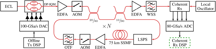
Figure 1: Experimental optical recirculating loop setup (ECL: external cavity laser, DP-IQ Mod: dual polarization IQ Modulator, EDFA: erbium-doped fiber amplifier, AOM: acousto-optic modulator, WSS: wavelength selective switch, DAC: digital-to-analog converter, ADC: analog-to-digital converter, DSP: digital signal processing, OTF: optical tunable filter, LSPS: loop-synchronized polarization scrambler, SSMF: standard single-mode fiber).

Figure 2: DSP chain applied to the digitized fiber output detected by the coherent receiver and analog-to-digital converter as shown in Fig. 1.

The complexity of LDBP can be reduced by applying model compression, which is commonly used in ML to reduce the size of NNs [27, 28]. In this paper, we use a simple pruning approach where the FIR filters are progressively shortened during SGD [26]. Our main finding is that the filters can be pruned to remarkably short lengths without sacrificing performance. As an example, consider single-channel DBP of a $10.7$-Gbaud signal over $25\times 80$ km of standard single-mode fiber (SSMF) using the SSFM with one step per span (StPS). For this scenario, Ip and Kahn have shown that $70$-tap filters are required to obtain acceptable accuracy [5]. This assumes that the filters are designed using FD sampling and that the same filter is used in each step. The resulting hardware complexity was estimated to be over $100$ times larger than for linear equalization. On the other hand, with jointly optimized filters, it was previously demonstrated that one can achieve similar accuracy by alternating between filters that are as short as $5$ and $3$ taps [25]. This reduces the complexity by almost two orders of magnitude, making it comparable to linear equalization in this case.

At first glance, it may not be clear why multi-step DBP can benefit from joint optimization of the filters. After all, the standard SSFM applies the same CD filter many times in succession, without the need for any elaborate optimization. The explanation is that in the presence of practical imperfections such as finite-length filter truncation, applying the same imperfect filter multiple times can be detrimental because it magnifies any weakness. To achieve a good combined response of neighboring filters and a good overall response, the truncation of each filter needs to be delicately balanced. For a more detailed discussion, we refer readers to [25, 41].

IV Experimental Results

For the experimental results presented in this section, our focus is on single-channel DBP of a polarization-multiplexed (PM) $25$ Gbaud signal over $1500$ km of SSMF. To obtain the results, we proceed in three steps:

1. Pre-train LDBP using data from split-step simulations and apply filter pruning to obtain short FIR filters in each step.

2. Fine-tune the model using pre-processed experimental data traces.

3. Test the fully-trained model on raw experimental data traces, by integrating LDBP into the receiver DSP chain.

The pre-processed experimental data traces mentioned in step 2 are obtained using the procedures described in Sec. IV-C. This pre-processing is necessary in order to provide LDBP with an estimation of effects such as phase noise and state of polarization. The raw experimental data traces in step 3 are the digital domain samples of the fiber output. These raw traces are processed by a different DSP chain, described in Sec. IV-A. In the following, we discuss each step in more detail, starting with the experimental testbed and DSP algorithms used for the experimental validation. Effective SNR is used throughout this section as the main figure of merit. We also note that the training procedure described in Sec. IV-B and Sec. IV-C is performed only once, since we only consider static effects, i.e., chromatic dispersion and fiber nonlinearities. Moreover, the trained model is independent of the transmitted power, as described in more detail below.

IV-A Recirculating Loop Setup and DSP Chain

A schematic of the experimental recirculating loop setup is depicted in Fig. 1. A total of 851 traces were captured in the launch power range of $-5$ dBm to $6$ dBm with steps of $0.5$ dBm, accounting for 37 traces per launch power. For each trace, we generate offline a sequence of $2^{16}$ symbols, using the Permuted Congruential Generator XSL RR 128/64 random number generator [42]. A new random seed is used for each sequence. The sequences are pulse-shaped using a root-raised cosine (RRC) filter with 1% roll-off, digitally pre-compensated for transmitter bandwidth limitations and uploaded to a 100-GSa/s digital-to-analog converter (DAC). The $193.4$ THz carrier is generated by an external cavity laser (ECL), modulated by a dual-polarization IQ-modulator (DP-IQM) and amplified using an erbium doped fiber amplifier (EDFA). Using acousto-optic modulators (AOMs), the optical signal is circulated in a recirculating loop consisting of a loop-synchronised polarization scrambler (LSPS), a 75-km span of SSMF, an EDFA and an optical tunable filter (OTF) for gain equalization.

At the receiver, the optical signal is amplified with an EDFA, filtered using a $50$ GHz optical bandwidth wavelength selective switch (WSS) and detected using an intradyne coherent receiver consisting of a local oscillator (LO), 90-degree hybrid and 4 balanced photodiodes with $43$ GHz electrical bandwidth. The resulting electrical signal is digitized by an 80-GSa/s real-time oscilloscope with an electrical bandwidth of $36$ GHz.

The receiver DSP consists of seven blocks, which are applied sequentially as represented in Fig. 2. Orthonormalization using blind moment estimation is applied to the signal for receiver optical front-end IQ compensation (gain imbalance and offset angle between the in-phase and quadrature components). Rational resampling to 2 samples per symbol is then applied. The next step is frequency-offset estimation and compensation to correct effects such as frequency difference between the local oscillator and the signal laser and frequency offsets introduced by the AOMs. After frequency-offset compensation, we apply either electronic dispersion compensation (EDC), DBP, or LDBP. The signal is then adaptively equalized and phase noise compensated. Here we use a MIMO equalizer trained with MSE metric. The MIMO equalizer is used to recover the signal state of polarization and partially compensate for other impairments, such as PMD. Within the update loop of the equalizer, blind phase search using the known transmitted symbols removes phase noise. The equalized signal is then downsampled to 1 sample per symbol and aligned with the transmitted sequence. Finally, the effective SNR is estimated.

IV-B Pre-Training and Filter Pruning

Simulations are used for pre-training where the simulation parameters are closely matched to the experimental setup. In particular, we assume single-channel transmission of a $25$ Gbaud signal (PM $16$-QAM, 1% RRC) over $20\times 75.484$ km of fiber ($\alpha=0.2$ dB/km, $\beta_{2}=-20.87$ ps²/km, $\gamma=1.3$ rad/W/km), where EDFAs (noise figure $5.0$ dB) compensate for attenuation after each span. Forward propagation is simulated with $300$ logarithmic StPS and $100$ GHz simulation bandwidth. No PMD or other hardware impairments are included in the simulations. At the receiver, the signal is low-pass filtered ($30$ GHz bandwidth) and downsampled to $2$ samples/symbol for further processing. LDBP is applied first, followed by a matched filter (MF) and phase-offset correction. LDBP is based on the symmetric SSFM using $3$ StPS and a logarithmic step size. When combining the adjacent linear half-steps, the overall model has $61$ linear steps. MSE is the loss function employed for training all FIR filters, defined as $\sum_{p\in\{\text{x},\text{y}\}}\lVert\boldsymbol{y}_{p}-\hat{\boldsymbol{y}}_{p}\rVert^{2}/2$, where $\boldsymbol{y}_{p}$ and $\hat{\boldsymbol{y}}_{p}$ are the transmitted and estimated symbol vectors of the $p$-polarization after the phase-offset correction, respectively. We assume that the filters are symmetric and that different filters are used in each polarization. This is essentially the same methodology as described in earlier work [23, 25].

Compared to most prior work on complexity-reduced DBP, it should be stressed that our goal is not to reduce the number of steps, but instead to reduce the per-step complexity. This is accomplished by employing filter pruning. All FIR filters are initialized with constrained least-squares CD coefficients according to [43]. The approach in [43] minimizes the frequency-response error of the FIR filter with respect to an ideal CD compensation filter within the signal bandwidth, while constraining the out-of-band filter gain. The initial filter lengths are chosen large enough to ensure good performance. The filters are then progressively pruned to a given target length by forcing the outermost taps to zero at certain iterations during SGD [26]. The zero forcing is done using a masking operation in TensorFlow. The iterations where pruning occurs are predefined before the training begins. For the considered scenario, the targeted model consisted of $22$ filters with $7$ taps and $39$ filters with $9$ taps. Training is performed for $50000$ iterations using the Adam optimizer [44], learning rate $0.0007$, and batch size $50$, which took around two hours on our machine. In principle, the number of iterations (and, hence, the training time) could be reduced, for example by setting a more aggressive learning rate. However, we observed that larger learning rates can sometimes lead to diverging MSE losses and numerical instabilities in our implementation. The filters are trained considering data from different launch powers, randomly chosen from the set $\mathcal{P}=\{1,1.5,2,2.5,3\}\,$dBm, resulting in a single model that tolerates changes in the input power.

IV-C Fine-Tuning with Experimental Data

The next step is to fine-tune the pre-trained and pruned LDBP model using experimental data traces. The key challenge when training with experimental data is the presence of various hardware impairments and time-varying effects such as PMD and carrier phase noise. Our approach is to first estimate these impairments using the conventional DSP chain and then properly pre-process the data. The actual training is then performed with the resulting pre-processed data. In particular:

• The received data samples are pre-processed by applying receiver front-end compensation and frequency-offset compensation. The frequency offset is estimated from the standard DSP chain. DBP is then applied to the resulting signal to improve the estimation of phase noise and the SOP.

• The data symbols used for supervised learning are circular-shifted for alignment with the data samples. These data symbols are pre-processed using the estimated phase noise process to de-rotate the symbols. More precisely, let $e^{\jmath\hat{\phi}_{i}}$ for $i=1,\ldots,N$ be the estimated phase noise process, where $N$ is the length of the data trace. Then, training is performed using the pre-processed symbols $e^{-\jmath\hat{\phi}_{i}}x_{i}$, $i=1,\ldots,N$, where $x_{i}$ are the true data symbols.

• Finally, the filter taps for the adaptive MIMO equalizer after the first $60000$ symbols are extracted and saved for each data trace. The equalizer is then assumed to be static for the rest of the trace. During LDBP training, the MIMO equalizer is integrated as a static DSP component after the MF, where the saved filter coefficients are loaded and applied. Note that the MIMO filter taps are not updated during the fine tuning of LDBP.

Fine-tuning using the above approach is performed for an additional $5000$ iterations using a learning rate $0.0007$, and batch size $50$. For training, we only consider 19 out of the 37 available traces for each launch power in the set $\mathcal{P}$, where the remaining traces are reserved for testing.

IV-D Testing

Figure 3: Experimental results for single-channel transmission of a $25\text{\,}\mathrm{G}\mathrm{b}\mathrm{a}\mathrm{u}\mathrm{d}$ signal with PM $16$-QAM over $1500\text{\,}\mathrm{k}\mathrm{m}$.

After fine-tuning is completed, the obtained model can then be used as a static nonlinear equalizer in the standard DSP chain described in Sec. IV-A (see middle block in Fig. 2). During the testing phase, all DSP blocks are operated normally and the raw (i.e., not pre-processed) experimental data is used. The obtained performance is shown in Fig. 3 with circle and diamond markers for EDC, standard DBP ($3$ StPS), and LDBP ($3$ StPS). For DBP, a well-known issue is that the nonlinearity parameter $\gamma$ is usually not known precisely and needs to be estimated [45]. We performed a simple grid search over $\gamma$, jointly with $\beta_{2}$, in order to optimize performance . For DBP with 3 StPS, the optimization was done at $2.5$ dBm launch power, which led to an optimal value of $\gamma=1.21$ rad/W/km and $\beta_{2}=-20.90$ ps²/km. The latter is close to the experimentally estimated $\beta_{2}=-20.87$ ps²/km. Similar to $\gamma$ and $\beta_{2}$, the fiber length is also usually not precisely determined. We already had an estimated measure of $75.484$ km for the span length, which was confirmed to be optimum after a grid search. The optimum attenuation coefficient for DBP was $\alpha=0.19$ dB/km, the same as in the fiber specifications. DBP with $3$ StPS achieves a peak-SNR gain of $2.1$ dB over EDC. The peak-SNR gain obtained by DBP is similar to those reported in prior experimental studies on single-channel DBP [46, 47]. DBP also improves the optimum launch power with respect to EDC by $4$ dB, from $-1.5$ dBm to $2.5$ dBm. By using LDBP, the peak-SNR gain is slighly increased with respect to DBP. Further increasing the number of StPS or filter taps for LDBP did not improve performance. The optimum launch power for LDBP remains the same as the one for DBP. We also repeated the same procedure assuming $1$ StPS for both DBP and LDBP, in which case the LDBP model uses $21$ filters per polarization, where $12$ filters are pruned to $23$ taps and $9$ filters to $21$ taps. The results in Fig. 3 (square markers) show that in this case LDBP achieves a performance improvement of around $0.35$ dB with respect to DBP. For DBP with 1 StPS, the optimum values for $\gamma$ and $\beta_{2}$ were found to be $\gamma=1.62$ rad/W/km and $\beta_{2}=-21.41$ ps²/km.

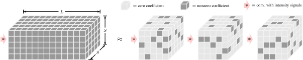
Figure 4: Tensor representation of an $L$-tap $S\times S$ MIMO filter for DBP based on subband processing, where $S$ is the number of subbands (left); learned multi-step decomposition with sparse subfilters (right).

In terms of complexity, it has been shown that the power consumption and chip area for time-domain DBP [48] and LDBP [26] are dominated by the linear steps, whereas the nonlinear steps have efficient hardware implementations using a Taylor expansion. Therefore, we focus on the linear steps for simplicity. As a simple surrogate measure for complexity, we use the overall impulse response length of the entire LDBP model, which is defined as the length of the filter obtained by convolving all LDBP subfilters. Since the same filter lengths are used in both polarizations, one may focus on a single polarization. For the $3$-StPS model, we have $22$ filters of length $7$ and $39$ filters of length $9$. Hence, the overall impulse response length is $2(22\cdot(7-1)/2+39\cdot(9-1)/2)+1=445$ taps. For the $1$-StPS model, the overall impulse response length is $2(12\cdot(23-1)/2+9\cdot(21-1)/2)+1=445$, i.e., the same as the $3$-StPS model. Thus, even though the number of steps is reduced by a factor of $3$ and performance decreases by around $0.3$ dB (see the inlet figure in Fig. 3), the expected hardware complexity of the two models is roughly comparable. Moreover, the overall impulse response lengths should be compared to the memory that is introduced by CD. To estimate the memory, one may use the fact that CD leads to a group delay difference of $2\pi|\beta_{2}|\Delta fL_{\text{tot}}$ over a bandwidth $\Delta f$ and transmission distance $L_{\text{tot}}$. Normalizing by the sampling interval $T$, this confines the memory to roughly $(2\pi|\beta_{2}|\Delta fL_{\text{tot}})/T$ samples. For our scenario, we have $\beta_{2}=-20.87$ ps²/km, $L_{\text{tot}}\approx 1510$ km, and $1/T=50$ GHz. The bandwidth $\Delta f$ depends on the baud rate, the pulse shaping filter, and the spectral broadening during propagation. In order to obtain an estimate for $\Delta f$, we quantified the effect of spectral broadening in an ideal noiseless simulation environment for the same parameters as listed in Sec. IV-B. The bandwidth percentage (with respect to $1/T$) that contained $99.9$% of the received signal power was found to vary between $51$% for $P=-4\,$dBm and $77$% for $P=6\,$dBm. With these numbers, the CD memory varies between $253$ and $381$ taps, which is comparable to the impulse response length of LDBP. This is a major improvement compared to previous work where the filter lengths in DBP are significantly longer than the CD memory, sometimes by orders of magnitude [5, 49]. We also note that it is possible to further prune the filters at the expense of some performance loss. To illustrate this, we further pruned the 3-StPS model to $22$ filters of length $5$ and $39$ filters of length $7$. This gave a peak-SNR penalty of $0.32$ dB (see Fig. 3), making the performance comparable to the $1$-StPS model, while at the same time reducing the overall impulse response length to only $323$ taps.

V Outlook and Future Work

In this section, we give an overview of related work on LDBP that has previously appeared in the literature and also comment on potentially interesting avenues for future work.

V-A Sparse MIMO Filters for Subband Processing

The complexity of DBP with TD filtering is largely dominated by the total number of required CD filter taps in all steps and this increases quadratically with bandwidth, see, e.g., [50, 51]. Thus, efficient TD-DBP of wideband signals is challenging. One possible solution is to employ subband processing and split the received signal into $S$ parallel signals using a filter bank [50, 51, 52, 53, 54, 55, 56, 57]. A theoretical foundation for DBP based on subband processing is obtained by inserting the split-signal assumption $u=\sum_{i=1}^{S}u_{i}$ into the NLSE. This leads to a set of coupled equations which can then be solved numerically. We focus on the modified SSFM proposed in [58] which is essentially equivalent to the standard SSFM for each subband, except that all sampled intensity waveforms $|u_{1}|^{2},\ldots,|u_{S}|^{2}$ are jointly processed with a MIMO filter prior to each nonlinear phase rotation step. This accounts for cross-phase modulation between subbands but not four-wave mixing because no phase information is exchanged.

The MIMO filters for subband processing can be relatively demanding in terms of hardware complexity. As an example, in [57] we considered a scenario where a $96$-Gbaud signal is split into $S=7$ subbands. For a filter length of $13$, the MIMO filter in each SSFM step can be represented as a $7\times 7\times 13$ tensor with $637$ real coefficients which is shown in Fig. 4 (left). The resulting complexity per step and subband would be almost $6$ times larger than that of the CD filters used in [57]. The situation can be improved significantly by decomposing each MIMO filter into a cascade of sparse filters as shown in Fig. 4 (right). For a cascade of $3$ filters, it was shown that a simple $L_{1}$-norm regularization applied to the filter coefficients during SGD leads to a sparsity level of round $8$%, i.e., $92$% of the filter coefficients can be set to zero with little performance penalty. Note that this filter decomposition happens within each SSFM step. In other words, complexity is reduced by further increasing the depth of the multi-step DBP computation graph.

V-B Distributed PMD Compensation

Different techniques have been proposed in previous works to embed the distributed compensation of PMD in the DBP algorithm, when the knowledge of the PMD evolution in the link is missing [37, 36, 59]. In this section, we describe how distributed PMD compensation can be combined with LDBP in a hardware-efficient manner.

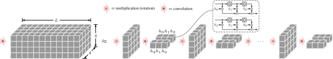
Figure 5: Tensor representation of an $L$-tap $4\times 4$ MIMO filter for PMD compensation (left); multi-step decomposition where $4$-D rotations are alternated with short fractional-delay (FD) filters accounting for DGD (right). Each FD filters is applied to both the real and imaginary part.

As discussed in Sec. II, PMD can be modeled by dividing a fiber link of length $L_{\text{tot}}$ into $M=L_{\text{tot}}/h$ sections, where for large enough $M$ the link Jones matrix $\mathbf{J}_{\text{Link}}(\omega)$ can be factorized as

$$\mathbf{J}_{\text{Link}}(\omega)\triangleq\exp\left(-j\omega\int_{0}^{L_{\text{tot}}}\Delta\beta^{\prime}(\xi)\overline{\boldsymbol{\sigma}}(\xi)d\xi\right)=\prod_{i=1}^{M}\mathbf{R}^{(i)}\mathbf{T}^{(i)}(\omega)$$ (11)

where $\mathbf{R}^{(i)}\triangleq\mathbf{R}(ih)$ and $\mathbf{T}^{(i)}(\omega)\triangleq\mathbf{T}(ih,\omega)$ for $i=1,2,\ldots,M$. PMD compensation (and polarization demultiplexing) then amounts to finding and applying the inverse $\mathbf{J}_{\text{Link}}^{-1}(\omega)$ to the received signal. This is typically performed after CD compensation, e.g., using an $L$-tap MIMO filter that tries to approximate $\mathbf{J}_{\text{Link}}^{-1}(\omega)$. Fig. 5 (left) shows the corresponding tensor representation assuming a real-valued $4\times 4$ filter that is applied to the separated real and imaginary parts of both polarizations [60].

An efficient multi-step decomposition of this filter is depicted in Fig. 5 (right), which essentially mimics (11) in a reverse fashion. Here, the matrices $\mathbf{T}^{(i)}(\omega)$ are approximated with two real-valued fractional-delay (FD) filters employing symmetrically flipped filter coefficients for different polarizations. The FD filters can be very short provided that the expected DGD per step is sufficiently small (i.e., many steps are used). In [61], it was shown how to integrate the decomposed filter structure into LDBP. The resulting multi-step PMD architecture can be trained effectively using SGD. An important feature compared to previous work is the fact that the employed approach does not assume any knowledge about the particular PMD realizations along the link, nor any knowledge about the total accumulated PMD. However, more research is needed to fully characterize the training behavior, e.g., in terms of convergence speed for adaptive compensation.

V-C Coefficient Quantization and ASIC Implementation

Fixed-point requirements and other DSP hardware implementation aspects for DBP have been investigated in [22, 26, 48, 49, 62]. A potential benefit of multi-step architectures is that they empirically tend to have many “good” parameter configurations that lie relatively close to each other. This implies that even if the optimized parameters are slightly perturbed (e.g., by quantizing them) there may exist a nearby parameter configuration that exhibits similarly good performance to mitigate the resulting performance loss due to the perturbation.

Numerical evidence for this phenomenon can be obtained by considering the joint optimization of CD filters in DBP including the effect of filter coefficient quantization. This has been studied in [26] and the approach relies on applying so-called “fake” quantizations to the filter coefficients, where the gradient computations and parameter updates during SGD are still performed in floating point. Compared to other quantization methods, this jointly optimizes the responses of quantized filters and can lead to significantly reduced fixed-point requirements. For the scenario in [26], it was shown for example that the bit resolution can be reduced from $8$-$9$ coefficient bits to $5$–$6$ bits without adversely affecting performance. Furthermore, hardware synthesis results in $28$-nm CMOS show that multi-step DBP based on TD filtering with short FIR filters is well within the limits of current ASIC technology in terms of chip area and power consumption [26, 48].

VI Conclusions

We have illustrated how machine learning can be used to achieve efficient fiber-nonlinearity compensation. Rather than reducing the number of steps (or steps per span), it was highlighted that complexity can also be reduced by carefully designing and optimizing multi-step methods, or even by increasing the number of steps and decomposing complex operations into simpler ones, without losing performance. We also avoided the use of neural networks as universal (but sometimes poorly understood) function approximators. Instead, the considered learned digital backpropagation relied on parameterizing the split-step method, i.e., an existing model-based algorithm. We have performed an experimental demonstration of this approach, which was shown to outperform standard digital backropagation with limited complexity. Some extensions of the approach and steps towards possible future works were also presented, showing that there is a possibility for further performance improvements in these systems.

References

- [1] E. Agrell, A. Alvarado, and F. R. Kschischang, “Implications of information theory in optical fibre communications,” Philosophical Transactions of the Royal Society A: Mathematical, Physical and Engineering Sciences, vol. 374, Mar. 2016.
- [2] G. Agrawal, Nonlinear Fiber Optics, 5th ed., ser. Optics and Photonics. Boston: Academic Press, 2013.
- [3] X. Li, et al., “Electronic post-compensation of WDM transmission impairments using coherent detection and digital signal processing,” Opt. Express, vol. 16, no. 2, pp. 880–888, Jan. 2008.
- [4] E. Mateo, L. Zhu, and G. Li, “Impact of XPM and FWM on the digital implementation of impairment compensation for WDM transmission using backward propagation,” Opt. Express, vol. 16, no. 20, pp. 16 124–16 137, Sept. 2008.
- [5] E. Ip and J. M. Kahn, “Compensation of dispersion and nonlinear impairments using digital backpropagation,” J. Lightw. Technol., vol. 26, no. 20, pp. 3416–3425, Oct. 2008.
- [6] D. S. Millar, et al., “Mitigation of fiber nonlinearity using a digital coherent receiver,” IEEE J. Sel. Topics. Quantum Electron., vol. 16, no. 5, pp. 1217–1226, Sept. 2010.
- [7] K. V. Peddanarappagari and M. Brandt-Pearce, “Volterra series transfer function of single-mode fibers,” J. Lightw. Technol., vol. 15, no. 12, pp. 2232–2241, Dec. 1997.
- [8] Y. Gao, F. Zhang, L. Dou, Z. Chen, and A. Xu, “Intra-channel nonlinearities mitigation in pseudo-linear coherent QPSK transmission systems via nonlinear electrical equalizer,” Opt. Communications, vol. 282, no. 12, pp. 2421–2425, 2009.
- [9] L. Liu, et al., “Intrachannel nonlinearity compensation by inverse Volterra series transfer function,” J. Lightw. Technol., vol. 30, no. 3, pp. 310–316, Feb. 2012.
- [10] F. P. Guiomar, J. D. Reis, A. L. Teixeira, and A. N. Pinto, “Mitigation of intra-channel nonlinearities using a frequency-domain Volterra series equalizer,” Opt. Express, vol. 20, no. 2, pp. 1360–1369, Jan. 2012.
- [11] W. Yan, et al., “Low complexity digital perturbation back-propagation,” in Proc. European Conf. Optical Communication (ECOC), Geneva, Switzerland, Sept. 2011.
- [12] Z. Tao, L. Dou, W. Yan, L. Li, T. Hoshida, and J. C. Rasmussen, “Multiplier-free intrachannel nonlinearity compensating algorithm operating at symbol rate,” J. Lightw. Technol., vol. 29, no. 17, pp. 2570–2576, Sept. 2011.
- [13] X. Liang and S. Kumar, “Multi-stage perturbation theory for compensating intra-channel nonlinear impairments in fiber-optic links,” Opt. Express, vol. 22, no. 24, p. 29733, Dec. 2014.
- [14] H. Nakashima, T. Oyama, C. Ohshima, Y. Akiyama, Z. Tao, and T. Hoshida, “Digital nonlinear compensation technologies in coherent optical communication systems,” in Proc. Optical Fiber Communication Conf. (OFC), Los Angeles, CA, 2017.
- [15] J. C. Cartledge, F. P. Guiomar, F. R. Kschischang, G. Liga, and M. P. Yankov, “Digital signal processing for fiber nonlinearities,” Opt. Express, vol. 25, no. 3, pp. 1916–1936, Feb. 2017.
- [16] L. B. Du and A. J. Lowery, “Improved single channel backpropagation for intra-channel fiber nonlinearity compensation in long-haul optical communication systems.” Opt. Express, vol. 18, no. 16, pp. 17 075–17 088, July 2010.
- [17] D. Rafique, M. Mussolin, M. Forzati, J. Mrtensson, M. N. Chugtai, and A. D. Ellis, “Compensation of intra-channel nonlinear fibre impairments using simplified digital back-propagation algorithm.” Opt. Express, vol. 19, no. 10, pp. 9453–9460, Apr. 2011.
- [18] A. Napoli, et al., “Reduced complexity digital back-propagation methods for optical communication systems,” J. Lightw. Technol., vol. 32, no. 7, pp. 1351–1362, Apr. 2014.
- [19] A. M. Jarajreh, et al., “Artificial neural network nonlinear equalizer for coherent optical OFDM,” IEEE Photon. Technol. Lett., vol. 27, no. 4, pp. 387–390, Feb. 2015.
- [20] E. Giacoumidis, et al., “Fiber nonlinearity-induced penalty reduction in CO-OFDM by ANN-based nonlinear equalization,” Opt. Lett., vol. 40, no. 21, pp. 5113–5116, Nov. 2015.
- [21] M. Secondini, S. Rommel, G. Meloni, F. Fresi, E. Forestieri, and L. Poti, “Single-step digital backpropagation for nonlinearity mitigation,” Photon. Netw. Commun., vol. 31, no. 3, pp. 493–502, 2016.
- [22] C. Fougstedt, M. Mazur, L. Svensson, H. Eliasson, M. Karlsson, and P. Larsson-Edefors, “Time-domain digital back propagation: algorithm and finite-precision implementation aspects,” in Proc. Optical Fiber Communication Conf. (OFC), Los Angeles, CA, 2017.
- [23] C. Häger and H. D. Pfister, “Nonlinear interference mitigation via deep neural networks,” in Proc. Optical Fiber Communication Conf. (OFC), San Diego, CA, 2018.
- [24] H. W. Lin, M. Tegmark, and D. Rolnick, “Why does deep and cheap learning work so well?” J. Stat. Phys., vol. 168, no. 6, pp. 1223–1247, Sept. 2017.
- [25] C. Häger and H. D. Pfister, “Deep learning of the nonlinear Schrödinger equation in fiber-optic communications,” in Proc. IEEE Int. Symp. Information Theory (ISIT), Vail, CO, 2018.
- [26] C. Fougstedt, C. Häger, L. Svensson, H. D. Pfister, and P. Larsson-Edefors, “ASIC implementation of time-domain digital backpropagation with deep-learned chromatic dispersion filters,” in Proc. European Conf. Optical Communication (ECOC), Rome, Italy, 2018.
- [27] Y. Lecun, J. S. Denker, and S. A. Solla, “Optimal Brain Damage,” in Proc. Advances in Neural Information Processing Systems (NIPS), Denver, CO, 1989.
- [28] S. Han, H. Mao, and W. J. Dally, “Deep compression: compressing deep neural networks with pruning, trained quantization and Huffman coding,” in Proc. Int. Conf. Learning Representations (ICLR), San Juan, Puerto Rico, 2016.
- [29] C. Häger, H. D. Pfister, R. M. Bütler, G. Liga, and A. Alvarado, “Revisiting multi-step nonlinearity compensation with machine learning,” in Proc. European Conf. Optical Communication (ECOC), Dublin, Ireland, 2019.
- [30] E. Sillekens, et al., “Experimental demonstration of learned time-domain digital back-propagation,” arXiv:1912.12197, Dec. 2019.
- [31] B. I. Bitachon, A. Ghazisaeidi, B. Baeuerle, M. Eppenberger, and J. Leuthold, “Deep Learning Based Digital Back Propagation with Polarization State Rotation & Phase Noise Invariance,” in Proc. Optical Fiber Communication Conf. (OFC), San Diego, CA, 2020.
- [32] D. Marcuse, C. R. Menyuk, and P. K. A. Wai, “Application of the Manakov-PMD equation to studies of signal propagation in optical fibers with randomly varying birefringence,” J. Lightw. Technol., vol. 15, no. 9, pp. 1735–1745, Sept. 1997.
- [33] E. Ip, “Nonlinear compensation using backpropagation for polarization-multiplexed transmission,” J. Lightw. Technol., vol. 28, no. 6, pp. 939–951, Mar. 2010.
- [34] R. Gilmore, “Baker-Campbell-Hausdorff formulas,” J. Mathematical Physics, vol. 15, no. 12, pp. 2090–2092, Dec. 1974.
- [35] O. V. Sinkin, R. Holzlohner, J. Zweck, and C. R. Menyuk, “Optimization of the split-step Fourier method in modeling optical-fiber communications systems,” J. Lightw. Technol., vol. 21, no. 1, pp. 61–68, Jan. 2003.
- [36] C. B. Czegledi, et al., “Digital backpropagation accounting for polarization-mode dispersion,” Opt. Express, vol. 25, no. 3, pp. 1903–1915, Feb. 2017.
- [37] G. Liga, C. Czegledi, and P. Bayvel, “A PMD-adaptive DBP receiver based on SNR optimization,” in Proc. Optical Fiber Communication Conf. (OFC), San Diego, CA, 2018.
- [38] S. J. Savory, “Digital filters for coherent optical receivers,” Opt. Express, vol. 16, no. 2, pp. 804–817, Jan. 2008.
- [39] L. Zhu, X. Li, E. Mateo, and G. Li, “Complementary FIR filter pair for distributed impairment compensation of WDM fiber transmission,” IEEE Photon. Technol. Lett., vol. 21, no. 5, pp. 292–294, Mar. 2009.
- [40] G. Goldfarb and G. Li, “Efficient backward-propagation using wavelet- based filtering for fiber backward-propagation,” Opt. Express, vol. 17, no. 11, pp. 814–816, May 2009.
- [41] M. Lian, C. Häger, and H. D. Pfister, “What can machine learning teach us about communications?” in Proc. IEEE Information Theory Workshop (ITW), Guangzhou, China, 2018.
- [42] M. E. O’Neill, “Pcg: A family of simple fast space-efficient statistically good algorithms for random number generation,” Harvey Mudd College, Claremont, CA, Tech. Rep. HMC-CS-2014-0905, Sept. 2014.
- [43] A. Sheikh, C. Fougstedt, A. Graell i Amat, P. Johannisson, P. Larsson-Edefors, and M. Karlsson, “Dispersion compensation FIR filter with improved robustness to coefficient quantization errors,” J. Lightw. Technol., vol. 34, no. 22, pp. 5110–5117, Nov. 2016.
- [44] D. P. Kingma and J. Ba, “Adam: a method for stochastic optimization,” in Proc. Int. Conf. Learning Representations (ICLR), San Diego, CA, 2015.
- [45] C.-Y. Lin, et al., “Adaptive digital back-propagation for optical communication systems,” in Proc. Optical Fiber Communication Conf. (OFC), San Franscisco, CA, 2014.
- [46] C. Lin, S. Chandrasekhar, and P. J. Winzer, “Experimental study of the limits of digital nonlinearity compensation in DWDM systems,” in Proc. Optical Fiber Communication Conf. (OFC), Los Angeles, CA, 2015.
- [47] L. Galdino, et al., “On the limits of digital back-propagation in the presence of transceiver noise,” Opt. Express, vol. 25, no. 4, pp. 4564–4578, Feb. 2017.
- [48] C. Fougstedt, L. Svensson, M. Mazur, M. Karlsson, and P. Larsson-Edefors, “ASIC implementation of time-domain digital back propagation for coherent receivers,” IEEE Photon. Technol. Lett., vol. 30, no. 13, pp. 1179–1182, July 2018.
- [49] C. S. Martins, L. Bertignono, A. Nespola, A. Carena, F. P. Guiomar, and A. N. Pinto, “Efficient time-domain DBP using random step-size and multi-band quantization,” in Proc. Optical Fiber Communication Conf. (OFC), San Diego, CA, 2018.
- [50] M. G. Taylor, “Compact digital dispersion compensation algorithms,” in Proc. Optical Fiber Communication Conf. (OFC), San Diego, CA, 2008.
- [51] K.-P. Ho, “Subband equaliser for chromatic dispersion of optical fibre,” Electronics Lett., vol. 45, no. 24, pp. 1224–1226, Nov. 2009.
- [52] I. Slim, A. Mezghani, L. G. Baltar, J. Qi, F. N. Hauske, and J. A. Nossek, “Delayed single-tap frequency-domain chromatic-dispersion compensation,” IEEE Photon. Technol. Lett., vol. 25, no. 2, pp. 167–170, Jan. 2013.
- [53] M. Nazarathy and A. Tolmachev, “Subbanded DSP architectures based on underdecimated filter banks for coherent OFDM receivers: Overview and recent advances,” IEEE Signal Processing Mag., vol. 31, no. 2, pp. 70–81, Mar. 2014.
- [54] E. F. Mateo, F. Yaman, and G. Li, “Efficient compensation of inter-channel nonlinear effects via digital backward propagation in WDM optical transmission,” Opt. Express, vol. 18, no. 14, pp. 15 144–15 154, July 2010.
- [55] E. Ip, N. Bai, and T. Wang, “Complexity versus performance tradeoff for fiber nonlinearity compensation using frequency-shaped, multi-subband backpropagation,” in Proc. Optical Fiber Communication Conf. (OFC), Los Angeles, CA, 2011.
- [56] T. Oyama, et al., “Complexity reduction of perturbation-based nonlinear compensator by sub-band processing,” in Proc. Optical Fiber Communication Conf. (OFC), Los Angeles, CA, 2015.
- [57] C. Häger and H. D. Pfister, “Wideband time-domain digital backpropagation via subband processing and deep learning,” in Proc. European Conf. Optical Communication (ECOC), Rome, Italy, 2018.
- [58] J. Leibrich and W. Rosenkranz, “Efficient numerical simulation of multichannel WDM transmission systems limited by XPM,” IEEE Photon. Technol. Lett., vol. 15, no. 3, pp. 395–397, Mar. 2003.
- [59] K. Goroshko, H. Louchet, and A. Richter, “Overcoming performance limitations of digital back propagation due to polarization mode dispersion,” in Proc. Int. Conf. Transparent Optical Networks (ICTON), Trento, Italy, 2016.
- [60] D. E. Crivelli, et al., “Architecture of a single-chip 50 Gb/s DP-QPSK/BPSK transceiver with electronic dispersion compensation for coherent optical channels,” IEEE Trans. Circuits Syst. I: Reg. Papers, vol. 61, no. 4, pp. 1012–1025, Apr. 2014.
- [61] C. Häger, H. D. Pfister, R. M. Bütler, G. Liga, and A. Alvarado, “Model-based machine learning for joint digital backpropagation and PMD compensation,” in Invited paper at the Optical Fiber Communication Conf. (OFC), San Diego, CA, 2020.
- [62] T. Sherborne, B. Banks, D. Semrau, R. I. Killey, P. Bayvel, and D. Lavery, “On the impact of fixed point hardware for optical fiber nonlinearity compensation algorithms,” J. Lightw. Technol., vol. 36, no. 20, pp. 5016–5022, Oct. 2018.