Non-locality and entanglement in multi- qubit systems from a unified framework

Abstract

Non-classical probability is the underlying feature of quantum mechanics. The emergence of Bell-CHSH non-locality for bipartite systems and linear entanglement inequalities for two-qubit systems has been shown in Adhikary et al. 2020 [Eur. Phys. J. D 74, 68 (2020)], purely as violations of classical probability rules. In this paper, we improve upon that work by showing that violation of any nonlocality inequality implies violation of classical probability rules, manifested through negative probabilities, without recourse to any underlying theory. Moving on to entanglement, we employ parent pseudoprojections to show how any number of linear and nonlinear entanglement witnesses for multiqubit systems can be obtained as violations of classical probability rules. They include the ones that have been derived earlier by employing different methods. It provides a perspective complementary to the current understanding in terms of the algebraic approaches.

1 Introduction

In quantum information, endeavour for identification of non-classical states has been motivated mainly by the non-classical applications that they offer. These applications are either altogether novel Bennett93 ; Ekert91 or show advantage over their classical counterparts Deutsch85 . Promising though these applications are, the true potential in various practical scenarios, such as conference quantum key distribution and multi-party quantum communication tasks can unravel in multi-party scenarios. So, various multi-partite generalisations of quantum communication protocols have been shown to this end Bouda01 ; Jian07 ; Epping17 . Non-classicality of correlations, e.g., non-locality Svetlichney87 , quantum entanglement Horodecki09 and quantum discord Ollivier01 acts as a resource in these applications. It has led to many criteria for detection of multiparty states possessing different features of nonclassicality Svetlichney87 ; Mermin90 ; Acin01 ; Seevinck02 ; Toth05 ; Guhne10 ; Vicente11 . The criteria are motivated from distinctive features of resource states (e.g., nonlocal and entangled states) vis-a-vis the so-called free states (e.g., local and separable states). Since there are many apparently different paradigms of (non-) classicality, the need for a common framework from which all the criteria of non-classicality are emergent becomes paramount.

Needless to mention, such a framework should rest on fundamental properties of quantum mechanics. As quantum mechanics is a new theory of probability Dirac42 ; Bartlett45 ; Feynman87 , violation of classical probability rules becomes an important avenue for emergence of various non-classicality criteria. In his seminal paper Fine82 , Fine has shown that the existence of joint probability distribution is equivalent to the condition of existence of hidden variable model, i.e., Bell inequality holds. Thus, nonlocality, a nonclassical feature not restricted only to quantum mechanics, can also be looked upon as the non-existence of joint probability distribution. Along the same lines, we show in this paper how nonlocality ineqaulities can be derived from violations of classical probability rules. We show that nonlocality leads to pseudoprobability scheme with negative entries (probabilities). This does not take recourse to any underlying physical theory. In fact, we present a formal proof that violation of any nonlocality inequality can be looked upon as a violation of classical probability sum rule. Existence of a nonnegative joint probability scheme would have precluded such a nonclassical behaviour.

Since entanglement is a nonclassical feature of quantum mechanics, in order to lay down an operational framework incorporating nonclassical probability, we introduced, in a recent work Adhikary20 , a new class of operators called pseudo projections. They are, by definition, quantum representatives of indicator functions for classical events in phase space. We showed that their expectation values – for a given state – have the significance of pseudo probabilities. When pseudo probabilities take values outside the interval $[0,1]$, they flag a non classical property of the underlying state. For, they essentially exhibit violations of classical probability rules.

A special case of interest is the Margenau Hill distribution Hill61 ; Barut88 , which is just the pseudo projection for the joint outcome of two observables (pseudo projections for outcomes of a single observable are always projections.). Employing just these minimal operators, we have recovered, in Adhikary20 , a number of non-classicality criteria which have been derived earlier from diverse considerations. They include Bell-CHSH inequality in any dimension and entanglement inequalities for two qubit states. In a subsequent work Asthana20 , we have further established the relationship between anomalous weak values and pseudo- probabilities. We have also derived conditions for quantum coherence in single qubit systems and quantum discord in two qubit systems. The generic nature of the framework gets manifested in that the criteria for so many different features of nonclassicality emerge from it as violations of classical probability rules.

In this paper, as a direct continuation of Adhikary20 ; Asthana20 , we answer the questions: (i) whether conditions for nonlocality and entanglement in multiparty and multiqubit systems respectively can also be looked upon as violations of classical probability rules and, (ii) how violation of classical probability rules can yield nonlinear entanglement inequalities in multi-qubit systems?

We employ our approach to unravel the violation of classical probability rules when the multi-party nonlocality inequalities derived in Svetlichney87 ; Mermin90 ; Seevinck02 ; Das17 get violated. Next, we show that multi-qubit entanglement inequalities, obtained in Acin01 ; Toth05 ; Guhne10 through various approaches, also emerge as violation of classical probability sum rules by employing pseudoprojections. In summary, we show that nonlocality leads to negative probabilities without any recourse to any physical theory, whereas entanglement leads to negative pseudoprobabilities constructed according to quantum mechanical rules.

The plan of the paper is as follows: For clarity and completeness, a brief account of the formalism for nonlocality and entanglement will be given in sections (2.1) and (2.2) respectively. We discuss relation of our work with the previous works in section (3). In section (4), we prove a central result, viz., violation of any condition for locality is concomitant on violation of a classical probability rule. We set up the notations in section (5) and explicitly identify pseudoprobabilities that turn negative for various multiparty nonlocality inequalities in section (6). Section (7) contains the results on entanglement. After describing the methodology to choose pseudoprobabilities for deriving entanglement inequalities in section (7.1), we present entanglement inequalities in sections (7.2- 7.4). In section (8), relative strengths of various inequalities are compared. Finally, section (9) summarises the paper.

2 The Formalism

In this section, we lay down the formalism to be employed for deriving nonlocality and entanglement inequalities as violations of classical probability rules. We first explicitly state the methodology employed for nonlocality.

2.1 Nonlocality

Nonlocality is a nonclassical feature not restricted to quantum mechanics. We start with a joint probability scheme without recourse to any physical model. We add suitably chosen entries from this scheme. Classically, this sum would have been nonnegative. We show that the conditions for nonlocality emerge when entries in the joint probability scheme turn negative. We term the joint probabilities as pseudoprobabilities, as they can take negative values. In section (4), we prove that violation of any nonlocality inequality always entails a sum of entries of underlying joint probability scheme to assume negative value.

2.2 Entanglement

In this section, we present the formalism to be employed for deriving sufficiency conditions for multiqubit entanglement. The pseudoprobabilities that we employ for obtaining entanglement inequalities are constructed using quantum mechanical rules.

The mathematical tool required for the formalism has been laid down in Adhikary20 . We recapitulate the formalism here for an uncluttered discussion.

2.2.1 Classical probability for an outcome of a single observable

Let there be a classical system in state $f$ and $M$ represents an observable taking values from the set $\{m_{i};i=1,2,\cdots\}$. In classical probability theory, in order to find the probability of an event $M=m_{i}$, one needs to identify the support $S^{M}_{m_{i}}$ for the event. Support is that region of event space in which the probability of happening of that event is 1. Thereafter, the overlap of the indicator function, $I_{S^{M}_{m_{i}}}$, constructed over the support $S^{M}_{m_{i}}$, with the state $f$ yields the probability of the event. Indicator functions are Boolean observables that assume value 1 inside the support and 0 outside it.

2.2.2 Extension to two observables

This method extends to more than one observable as well. For example, let there be two observables $M,N$ taking values in the sets $\{m_{i};i=1,2,\cdots\}$ and $\{n_{j};j=1,2,\cdots\}$. The overlap of the indicator function constructed over the intersection of the supports of the two events, ${S^{M}_{m_{i}}}$ and ${S^{N}_{n_{j}}}$, with the state $f$ yields the probability for the event $M=m_{i}$ and $N=n_{j}$.

2.2.3 Quantum representatives of indicator functions for joint events: Pseudoprojections

While transiting to quantum mechanics, observables map to hermitian operators. Indicator functions for different outcomes of a given observable map to projections of the hermitian operators with the corresponding eigenvalues. The crux of the matter is that indicator functions for joint outcomes of two or more observables do not map to projection operators, unless the observables commute. Such indicator functions for the joint outcomes of multiple observables map to pseudo projections Adhikary20 , which are symmetrised products of the individual projections. By construction, pseudo projections are hermitian, but not idempotent. Nor are their spectrums bounded in the unit interval $[0,1]$, unlike their parent indicator functions. Violation of this classical bound is the source of non-classicality in quantum mechanics.

Consider, for instance, the two observables $M,N$ and let $\pi_{m_{i}},~{}\pi_{n_{j}}$ be the projection operators representing the respective indicator functions for the outcomes $M=m_{i}$ and $N=n_{j}$. The operator, i.e., the pseudo-projection representing the classical indicator function for their joint outcome is the symmetrised product Hill61 ; Barut88 :

$$\mathbf{\Pi}_{m_{i}n_{j}}=\frac{1}{2}\Big{\{}\pi_{m_{i}},\pi_{n_{j}}\Big{\}},$$ (1)

in accordance with Weyl ordering Weyl27 .

2.2.4 Pseudoprojection for joint outcomes of more than two observables

Pseudoprojections representing joint outcomes of more than two observables can also be constructed similarly. For example, consider the joint outcomes, $O_{1}=o_{1},\cdots,O_{N}=o_{N}$, of $N$ observables. If $\pi_{o_{i}}$ represents the projection for $O_{i}=o_{i}$, their product can be permuted, in general, in $N!$ ways. If all the projections happen to be distinct from each other, this will give rise to $N!/2$ quantum representatives of the form

$${\bf\Pi}_{o_{1}\cdots o_{N}}=\dfrac{1}{2}\big{(}\pi_{o_{1}}\cdots\pi_{o_{N}}+{\rm h.~{}c.}\big{)},$$ (2)

where ${\rm h.c.}$ represents hermitian conjugate. A pseudoprojection obtained from a given order of $N$ distinct projections is termed as unit pseudoprojction.

All $N!/2$ unit pseudoprojections are legitimate quantum representatives of the same classical indicator function. For this reason, one may consider their convex sums, which will also be equally valid quantum representatives of classical indicator function.

2.2.5 Pseudoprobability in quantum mechanics

The overlap of a pseudoprojection with a state $\rho$ is defined to be pseudo-probability, i.e., the pseudo-probability ${\cal P}_{o_{1}\cdots o_{N}}$ for joint outcomes of $O_{1}=o_{1},\cdots,O_{N}=o_{N}$ in a state $\rho$ is defined as,

$${\cal P}_{o_{1}\cdots o_{N}}\equiv{\rm Tr}({\bf\Pi}_{o_{1}\cdots o_{N}}\rho).$$ (3)

Pseudoprojections for a multipartite system are direct products of those for single subsystems.

Only a pseudo-projection involving mutually commuting projections is a true projection, whence its expectation value in any state necessarily possesses an interpretation of being a probability. More generally, if we were to construct a scheme of joint pseudo-probabilities (PPS), involving all possible outcomes of each observable, then only the marginals, involving only sets of mutually commuting observables, are guaranteed to have the character of a classical probability scheme – with entries in agreement with the predictions of quantum mechanics.

This leads to a broad definition of non-classicality of a state with respect to a given set of observables Adhikary20 .

2.2.6 Nonclassicality of quantum states

Definition: A quantum state is nonclassical if even one pseudo-probability in the PPS is negative.

This definition is more general than the ones given in Hill61 ; Barut88 ; Johansen_04 ; Pusey14 since it incorporates pseudo-probabilities generated by pseudo-projections for joint outcomes of any number of observables and by convex sums of unit pseudoprojections as well. The sum of a chosen set of pseudoprobabilities of a scheme may also assume value outside [0, 1] and may act as an independent signature of nonclassicality.

Indeed, PPS, is of fundamental importance. If all the entries in a PPS turn to be non-negative, it will be equivalent to a classical joint probability scheme; there would be no non classicality. This leads us to conjecture that pseudoprobabilities capture all the nonclassical features of quantum mechanics. If this be so, one must recover the conditions for various manifests of nonclassicality in quantum mechanics, in particular, entanglement in multi-qubit systems from pseudoprobabilities. In section (7), we show that it is indeed so.

Before we move to our main results, we make a comparison between our work and the previous works in the next section.

3 Relation with previous works

Historically, we note that the product of noncommuting projections was first employed by Kirkwood Kirkwood33 and Barut Barut57 for construction of a complex probability distribution. Later, Margenau and Hill Hill61 , and Barut et al.Barut88 employed the hermitized product for construction of a quasiprobability distribution of joint outcome of non-commuting operators. Such a distribution has been used in Puri12 to characterise nonclassical correlations of multiqubit system with prior knowledge of average direction of single subsystem. The present approach starts with the more fundamental indicator functions, and systematically provides conditions for non-classicality purely as violations of classical probability rules. This, to the best of our knowledge, has not been explored before.

In this paper, we are interested in two specific forms of nonclassicality: nonlocality in multiparty systems and entanglement in multiqubit systems. The conditions for multiparty nonlocality have earlier been derived assuming (i) hybrid local-nonlocal models Svetlichney87 ; Seevinck02 and (ii) completely factorisable local hidden variable model Mermin90 . In this paper, we show that conditions for nonlocality emerge when there are negative entries in the underlying joint probability scheme. The two approaches are dual to each other, as shown by Fine for Bell inequality Fine82 . In fact, our approach gives a mathematical framework to the hidden variable models and those models provide a physical basis for our appraoch.

Conditions for different kinds of multiqubit entanglement have earlier been obtained through (i) conditions on entries of density matrices of biseparable and completely separable states vis-a-vis entangled states Guhne10 , (ii) stabiliser formalism Toth05 , (iii) witnesses involving projection operators for entangled states Acin01 , to name a few. In contrast, in our work, we show that all these conditions can be arrived at purely by looking at violation of classical probability rules through pseudoprobabilties in quantum mechanics.

4 Violation of any linear nonlocality inequality implies violation of a classical probability rule

In this section, we prove that violation of any linear nonlocality inequality is equivalent to the nonexistence of an underlying classical joint probability scheme. We show it for a bipartite system but the proof admits a straightforward generalisation to multipartite systems as well.

4.1 Condition for locality

Let $\{C_{\alpha}\}$ and $\{D_{\beta}\}$ be sets of $N_{1}$ and $N_{2}$ observables for the first and the second subsystems of a bipartite system respectively. The respective sets of outcomes of the observables $C_{\alpha}$ and $D_{\beta}$ are represented by $\{c_{\alpha}^{i_{\alpha}}\}$ and $\{d_{\beta}^{j_{\beta}}\}$. If ${\cal P}(C_{\alpha}=c^{i_{\alpha}}_{\alpha};D_{\beta}=d_{\beta}^{j_{\beta}})$ represents the probability for the joint event $C_{\alpha}=c_{\alpha}^{i_{\alpha}}$ and $D_{\beta}=d_{\beta}^{j_{\beta}}$, a linear nonlocality inequality obeyed by local hidden variable models Brunner14 would read as follows:

$${\cal I}\equiv\sum_{\alpha\beta}\sum_{i_{\alpha}j_{\beta}}w^{\alpha\beta}_{i_{\alpha}j_{\beta}}{\cal P}(C_{\alpha}=c^{i_{\alpha}}_{\alpha};D_{\beta}=d^{j_{\beta}}_{\beta})\leq R.$$ (4)

We can take all the coefficients $w^{\alpha\beta}_{i_{\alpha}j_{\beta}}\geq 0$, for if any of them were negative, we rewrite the corresponding ${\cal P}$ as $1-{\cal P}^{\prime}$, where ${\cal P}^{\prime}$ is the probability for the complementary event. This implies the existence of an upper bound $R\geq 0$ for all local hidden variable models.

Lemma: Let ${\cal M}_{1},{\cal M}_{2},\cdots$ be the sets of all mutually consistent events $\{C_{\alpha}=c^{i_{\alpha}}_{\alpha};D_{\beta}=d_{\beta}^{j_{\beta}}\}$, and let ${\cal N}_{1},{\cal N}_{2},\cdots$ represent the sets of corresponding coefficients $w^{\alpha\beta}_{i_{\alpha}j_{\beta}}$ in inequality $(\ref{Nonlocality})$. Mutually consistent events imply the events that can be simultaneously assigned probability equal to one in a local hidden variable model. If, for a given ${\cal N}_{k}$, the sum of all coefficients $w^{\alpha\beta}_{i_{\alpha}j_{\beta}}\in{\cal N}_{k}$ is $R_{k}$, then,

$$R\geq\underset{\{{\cal N}_{k}\}}{\max}R_{k},$$ (5)

where the maximum is taken over all ${\cal N}_{1},{\cal N}_{2},\cdots$.

Proof: For a given $k$, there always exists a local hidden variable model in which all the events belonging to the set ${\cal M}_{k}$ can be assigned unit probability, and all the events inconsistent with the events belonging to ${\cal M}_{k}$ have zero probability. Since $k$ is an arbitrary label and the inequality (4) is obeyed by all the local hidden variable models, equation (5) holds.

Theorem 1: Violation of the inequality (4) implies violation of a classical probability rule.
Proof: We prove by contradiction. Assume that there exists an underlying nonnegative joint probability scheme,

$$\Big{\{}{\cal P}\Big{(}C_{1}=c_{1}^{i_{1}},\cdots,C_{N_{1}}=c_{N_{1}}^{i_{N_{1}}};D_{1}=d_{1}^{j_{1}},\cdots,D_{N_{2}}=d_{N_{2}}^{j_{N_{2}}}\Big{)}\Big{\}},$$

which we compactly represent as $\{{\cal P}\big{(}\{C_{\alpha}=c_{\alpha}^{i_{\alpha}}\};\{D_{\beta}=d_{\beta}^{j_{\beta}}\}\big{)}\}$. Consider the expression

$$R-{\cal I}= R-\sum_{\alpha\beta}\sum_{i_{\alpha}j_{\beta}}w^{\alpha\beta}_{i_{\alpha}j_{\beta}}{\cal P}(C_{\alpha}=c_{\alpha}^{i_{\alpha}};D_{\beta}=d_{\beta}^{j_{\beta}}),$$

which we rewrite as $R\cdot 1-{\cal I}$, where we insert the sum rule for joint probabilities,

$$\sum_{\begin{subarray}{c}i_{1}\cdots i_{N_{1}}\\ j_{1}\cdots j_{N_{2}}\end{subarray}}{\cal P}\big{(}\{C_{\alpha}=c_{\alpha}^{i_{\alpha}}\};\{D_{\beta}=d_{\beta}^{j_{\beta}}\}\big{)}=1,$$ (6)

Thus,

$$R-{\cal I}$$

$$=R\sum_{\begin{subarray}{c}i_{1}\cdots i_{N_{1}}\\ j_{1}\cdots j_{N_{2}}\end{subarray}}{\cal P}\big{(}\{C_{\alpha}=c_{\alpha}^{i_{\alpha}}\};\{D_{\beta}=d_{\beta}^{j_{\beta}}\}\big{)}-\sum_{\alpha\beta}\sum_{\begin{subarray}{c}i_{1}\cdots i_{N_{1}}\\ j_{1}\cdots j_{N_{2}}\end{subarray}}w^{\alpha\beta}_{i_{\alpha}j_{\beta}}{\cal P}\big{(}\{C_{\alpha}=c_{\alpha}^{i_{\alpha}}\};\{D_{\beta}=d_{\beta}^{j_{\beta}}\}\big{)}.$$ (7)

The proof follows by employing the inequality in equation (5). Since only mutually consistent events in a local hidden variable model have common joint events, the coefficient of a given joint probability ${\cal P}\big{(}\{C_{\alpha}=c_{\alpha}^{i_{\alpha}}\};\{D_{\beta}=d_{\beta}^{j_{\beta}}\}\big{)}$ in the second term of equation (7) equals $R_{k}$, for some $k$. So, equation (7) contains the sum of joint probabilities with nonnegative coefficients. If, in addition, all the joint probabilities were to be nonnegative, it would follow that,

$$R-\sum_{\alpha\beta}\sum_{i_{\alpha}j_{\beta}}w^{\alpha\beta}_{i_{\alpha}j_{\beta}}{\cal P}(C_{\alpha}=c_{\alpha}^{i_{\alpha}};D_{\beta}=d_{\beta}^{j_{\beta}})\geq 0,$$ (8)

which agrees with the locality condition (4). Thus, a violation of inequality (4) is possible only if the weighted sum of joint probabilities given in equation (7) is negative. This, in turn, implies that in place of joint probabilities, we have pseudoprobabilities that assume negative values as well. The validity of the result is not restricted to linear nonlocality inequalities. That it can be extended to nonlinear nonlocality inequalities is shown in Appendix (A).

Theorem 1 and 1A (proved in Appendix (A)) provide the formal basis for our constructions of combinations of pseudoprobabilities to exhibit violations of classical probability rules. In this paper, we shall focus our attention exclusively on nonlocality and entanglement inequalities in multiparty and multiqubit systems respectively.

5 Notations

In this section, we setup compact notations to be used henceforth in the paper for expressing the results. This is made possible because we employ only dichotomic observables, with outcomes $\pm 1$.

1. The symbol ${\cal E}$ is reserved to denote events.

2. Recall that the symbol ${\cal P}$ has a dual significance: it represents pseudoprobabilities for joint outcomes of observables for nonlocality, which can assume both negative and nonnegative values. For entanglement, it represents pseudo probabilities, defined as expectations of the pseudoprojections for the corresponding joint events.

3. $\mathcal{E}(A=+1)\equiv\mathcal{E}(A)$, and its negation, $\mathcal{E}(A=-1)\equiv\mathcal{E}({\bar{A}})$.

4. For an $N$ party system, the observable $A_{i}$ refers to the $i^{th}$ subsystem. Observables belonging to the same subsystem are distinguished by primes in the superscript, such as $A^{\prime}_{i},~{}A^{\prime\prime}_{i},\cdots$.

5. The pseudo-probability for a joint event ${\cal E}(A_{1}=+1,A^{\prime}_{1}=+1;A_{2}=+1,A^{\prime}_{2}=-1)$ is represented compactly as $\mathcal{P}(A_{1}A^{\prime}_{1};A_{2}{\bar{A}}^{\prime}_{2})$. This rule admits easy generalisation.

6. The pseudo probability $\mathcal{P}(A_{1}=A^{\prime}_{1})$ represents the sum $\mathcal{P}(A_{1}A^{\prime}_{1})+\mathcal{P}(\bar{A}_{1}\bar{A}^{\prime}_{1})$.

7. The compact notation ${\cal P}({\cal E};A)$ represents the pseudo-probability for the joint occurrence of event ${\cal E}$ together with $A=+1$.

8. The symbol $\vee$ is employed for standard OR operation. Since, we use mutually exclusive events, so

   $${\cal P}({\cal E}_{1}\vee{\cal E}_{2})={\cal P}({\cal E}_{1})+{\cal P}({\cal E}_{2}),$$

   for any two events ${\cal E}_{1}$ and ${\cal E}_{2}$.

9. As an exception, we employ lower case letters for the observables of a qubit: $A_{i}\rightarrow a_{i}\equiv\vec{\sigma}_{i}\cdot\hat{a}_{i}$.

6 Multiparty non-locality

Equipped with the result of section (4), we apply the framework to multiparty nonlocality. Combinations of appropriate pseudoprobabilities of a joint pseudoprobability scheme yield us the required inequality. Furthermore, we reexpress the pseudoprobabilities in terms of expectations of observables, that can be experimentally measured.

6.1 Svetlichny Inequality

Svetlichny inequality detects $N$– party nonlocal correlations that are not reducible to ($N-M$) party correlations related locally to the rest of $M$–parties ($M<N$). For illustration, we consider the simplest case of three party system first.

6.1.1 N=3

Of relevance to this example is the specific sum of pseudoprobabilities, given by

$${\cal P}_{3}^{S}\equiv \mathcal{P}({\cal E}_{2}^{\alpha};A^{\prime}_{3})+\mathcal{P}({\cal E}_{2}^{\alpha^{\prime}};{\bar{A}}^{\prime}_{3})+\mathcal{P}({\cal E}_{2}^{\beta};A_{3})+\mathcal{P}({\cal E}_{2}^{\beta^{\prime}};{\bar{A}}_{3}),$$ (9)

where the event ${\cal E}_{2}^{\alpha}$ is the event underlying the Bell CHSH inequality for the residual two party subsystem:

$${\cal E}_{2}^{\alpha}\equiv{\cal E}({\bar{A}}_{1}=A^{\prime}_{1}=A_{2})\vee{\cal E}(A_{1}=A^{\prime}_{1}=A^{\prime}_{2}).$$ (10)

The other three events, again for the residual two party systems, are obtained via the transformations of observables as shown in table (1).

Events	Observables
${\cal E}_{2}^{\alpha}\rightarrow{\cal E}_{2}^{\beta}$	Interchange of primed and unprimed observables
${\cal E}_{2}^{\alpha}\rightarrow{\cal E}_{2}^{\alpha^{\prime}}$ ${\cal E}_{2}^{\beta}\rightarrow{\cal E}_{2}^{\beta^{\prime}}$	$A_{2}\leftrightarrow{\bar{A}}_{2};~{}A^{\prime}_{2}\leftrightarrow{\bar{A}}^{\prime}_{2}$

Table 1: Transformation of events and corresponding transformation of observables.

We write the pseudoprobabilities in terms of expectations of observables by employing the sum rule for pseudoprobabilities and dichotomic nature of the observables (see Appendix (B) for derivation). The demand that ${\cal P}_{3}^{S}<0$, which is forbidden classically, gives rise to the inequality

$$\langle S_{3}\rangle= \Big{\langle}\big{\{}(-A_{1}+A^{\prime}_{1})A_{2}+(A_{1}+A^{\prime}_{1})A^{\prime}_{2}\big{\}}A^{\prime}_{3}$$

$$+ \big{\{}(A_{1}+A^{\prime}_{1})A_{2}+(A_{1}-A^{\prime}_{1})A^{\prime}_{2}\big{\}}A_{3}\Big{\rangle}<-4$$ (11)

If we now interchange ${\bar{A}}_{1}$ and ${\bar{A}}^{\prime}_{1}$ with $A_{1}$ and $A^{\prime}_{1}$ respectively in equation (9), we obtain the complementary condition $\langle S_{3}\rangle>4$ which, combined with (6.1.1), yields the simplest Svetlichny inequality,

$${\cal I}_{S_{3}}:~{}|\langle S_{3}\rangle|= \Big{|}\Big{\langle}\big{\{}(-A_{1}+A^{\prime}_{1})A_{2}+(A_{1}+A^{\prime}_{1})A^{\prime}_{2}\big{\}}A^{\prime}_{3}$$

$$+ \big{\{}(A_{1}+A^{\prime}_{1})A_{2}+(A_{1}-A^{\prime}_{1})A^{\prime}_{2}\big{\}}A_{3}\Big{\rangle}\Big{|}>4$$ (12)

6.1.2 $N$-party system

The above approach suggests construction of pseudo probabilities to set up Svetlichny inequality for an $N$– party system. It is identified to be the sum, recursively defined in terms of $(N-1)$ party events, given by

$${\cal P}^{S}_{N}\equiv \mathcal{P}({\mathcal{E}_{N-1}^{\alpha}};A^{\prime}_{N})+\mathcal{P}(\mathcal{E}_{N-1}^{\alpha^{\prime}};{\bar{A}}^{\prime}_{N})+\mathcal{P}(\mathcal{E}_{N-1}^{\beta};A_{N})+\mathcal{P}(\mathcal{E}_{N-1}^{\beta^{\prime}};{\bar{A}}_{N});N\geq 3.$$ (13)

The associated event ${\cal E}^{\alpha}_{N}$ is given, recursively by

$${\cal E}^{\alpha}_{N}\equiv {\cal E}({\mathcal{E}_{N-1}^{\alpha}};A^{\prime}_{N})\vee{\cal E}(\mathcal{E}_{N-1}^{\alpha^{\prime}};{\bar{A}}^{\prime}_{N})\vee{\cal E}(\mathcal{E}_{N-1}^{\beta};A_{N})\vee{\cal E}(\mathcal{E}_{N-1}^{\beta^{\prime}};{\bar{A}}_{N});$$ (14)

The elementary event ${\cal E}_{2}^{\alpha}$ is defined in equation (10). The other events – ${\cal E}_{N-1}^{\alpha^{\prime}},{\cal E}_{N-1}^{\beta},{\cal E}_{N-1}^{\beta^{\prime}}$, can be obtained by changing the observables, as prescribed in table (2).

Events	Observables
${\cal E}_{N-1}^{\alpha}\rightarrow{\cal E}_{N-1}^{\beta}$	Change primed and unprimed observables.
${\cal E}_{N-1}^{\alpha}\rightarrow{\cal E}_{N-1}^{\alpha^{\prime}}$ ${\cal E}_{N-1}^{\beta}\rightarrow{\cal E}_{N-1}^{\beta^{\prime}}$	$A_{N-1}\leftrightarrow{\bar{A}}_{N-1}$ and $A^{\prime}_{N-1}\leftrightarrow{\bar{A}}^{\prime}_{N-1}$

Table 2: Transformation of events and corresponding transformation of observables.

After writing pseudoprobabilities in terms of expectations of observables, the non classicality condition, ${\cal P}^{S}_{N}<0$, straightaway yields the inequality (obtained in Bancal11 , by an entirely different method):

$${\cal I}_{S_{N}}:~{}\langle S_{N-1}A^{\prime}_{N}+S^{\prime}_{N-1}A_{N}\rangle<-2^{N-1},$$ (15)

where $S_{N-1}$ is the Svetlichny polynomial for the $(N-1)$–party system; $S^{\prime}_{N-1}$ can be obtained from $S_{N-1}$ by interchanging the primed and the unprimed observables.

6.2 Das-Datta-Agrawal inequalities.

Recently, Das et al. Das17 derived an inequality for three party systems, by combining Bell inequalities for the constituent two party subsystems. The inequality was tested against the so called generalised GHZ states, and subsequently generalised to multiparty states. Here, the stringent condition on correlations, imposed while deriving Svetlichny inequality, is relaxed to admit the existence of correlations involving $(N-1)$ parties as well. As promised, we recover them as violations of appropriate classical probability rules. We start with the simplest case.

6.2.1 $N$=3

We start with the sum of pseudo-probabilities,

$${\cal P}^{D}_{3}\equiv {\cal P}({\cal E}_{3}^{\alpha})+{\cal P}({\cal E}_{3}^{\beta}),$$ (16)

for the events

$${\cal E}_{3}^{\alpha} \equiv{\cal E}(A_{1}=A^{\prime}_{1}=A_{2};A_{3})\vee{\cal E}(A_{1}=A^{\prime}_{1}={\bar{A}}_{2};{\bar{A}}_{3});$$

$${\cal E}_{3}^{\beta} \equiv{\cal E}(A_{1}={\bar{A}}^{\prime}_{1}=A^{\prime}_{2}).$$ (17)

Again after writing the pseudoprobabilities in terms of expectations of the observables, the non-classicality condition, ${\cal P}_{3}^{D}<0$, yields the inequality

$$\big{\langle}(A_{1}+A^{\prime}_{1})A_{2}A_{3}+(A_{1}-A^{\prime}_{1})A^{\prime}_{2}\big{\rangle}<-2.$$ (18)

which, as we may see, involves two party correlators also. Furthermore, it does not treat all the subsystems on par. As in the previous subsection, the generalization to an $N$ party system is straightforward, except that we need to distinguish the two cases, viz., $N$ even or odd.

6.2.2 $N$ even

The relevant sum of pseudo probabilities is defined recursively, by

$${\cal P}^{D}_{N}\equiv {\cal P}({\cal E}_{N}^{\alpha})+{\cal P}({\cal E}_{N}^{\beta});N\geq 4,$$ (19)

where

$${\cal E}_{N}^{\alpha} \equiv{\cal E}({\cal E}_{N-1}^{\alpha};A_{N})\vee{\cal E}({\cal E}_{N-1}^{\alpha^{\prime}};{\bar{A}}_{N});$$

$${\cal E}_{N}^{\beta} \equiv{\cal E}({\cal E}_{N-1}^{\gamma};A^{\prime}_{N})\vee{\cal E}({\cal E}_{N-1}^{\gamma^{\prime}};{\bar{A}}^{\prime}_{N}),$$ (20)

where ${\cal E}_{N-1}^{\gamma}\equiv{\cal E}({\cal E}^{\beta}_{N-1};A^{\prime}_{N-1})\vee({\cal E}^{\beta^{\prime}}_{N-1};{\bar{A}}^{\prime}_{N-1})$. The transformations required to obtain ${\cal E}^{\alpha^{\prime}}_{N-1}$, ${\cal E}^{\beta^{\prime}}_{N-1}$ and ${\cal E}^{\gamma^{\prime}}_{N-1}$ from ${\cal E}^{\alpha}_{N-1},{\cal E}^{\beta}_{N-1}$ and ${\cal E}^{\gamma}_{N-1}$ respectively are shown in table (3).

Events	Observables
${\cal E}_{N-1}^{\alpha}\rightarrow{\cal E}_{N-1}^{\alpha^{\prime}}$	$A_{N-1}\leftrightarrow{\bar{A}}_{N-1}$
${\cal E}_{N-1}^{\beta}\rightarrow{\cal E}_{N-1}^{\beta^{\prime}}$	$A^{\prime}_{N-2}\leftrightarrow{\bar{A}}^{\prime}_{N-2}$
${\cal E}_{N-1}^{\gamma}\rightarrow{\cal E}_{N-1}^{\gamma^{\prime}}$	$A^{\prime}_{N-1}\leftrightarrow{\bar{A}}^{\prime}_{N-1}$

Table 3: Transformation of events and corresponding transformation of observables.

After plugging in the expressions of pseudoprobabilities in terms of expectations, the condition ${\cal P}^{D}_{N}<0$, translates to the inequality

$$\big{\langle}(A_{1}+A^{\prime}_{1})A_{2}\cdots A_{N}+(A_{1}-A^{\prime}_{1})A^{\prime}_{2}\cdots A^{\prime}_{N}\big{\rangle}<-2.$$ (21)

It may be noted that every term has the full $N$ party correlation.

6.2.3 $N$ odd

The pseudo probability that we need is

$${\cal P}^{D}_{N}\equiv {\cal P}({\cal E}^{\alpha}_{N})+{\cal P}({\cal E}^{\beta}_{N});N\geq 5,$$ (22)

where the events,

$${\cal E}^{\alpha}_{N}\equiv{\cal E}({\cal E}^{\alpha}_{N-1};A_{N})\vee{\cal E}({\cal E}^{\alpha^{\prime}}_{N-1};{\bar{A}}_{N});{\cal E}^{\beta}_{N}\equiv{\cal E}^{\beta}_{N-1}.$$ (23)

The event ${\cal E}^{\alpha^{\prime}}_{N-1}$ can be obtained from ${\cal E}^{\alpha}_{N-1}$ by the interchange $A_{N-1}\leftrightarrow{\bar{A}}_{N-1}$. After writing the pseudoprobabilities in terms of expectations of observables and imposing the nonclassicality condition ${\cal P}^{D}_{N}$, the ensuing inequality reads as

$$\big{\langle}(A_{1}+A^{\prime}_{1})A_{2}\cdots A_{N}+(A_{1}-A^{\prime}_{1})A^{\prime}_{2}\cdots A^{\prime}_{N-1}\big{\rangle}<-2$$ (24)

which also gets a contribution from $(N-1)$ party correlators.

6.3 Mermin-Ardehali Inequality

Mermin derived an inequality for a completely factorisable local hidden variable model for correlations of $N$–party statesMermin90 . We present the results, first for three party system and subsequently, for $N$ party systems. These inequalities also differ for $N$ even and $N$ odd, and are expressed in terms of the Mermin polynomial $M_{N}$, defined recursively by $M_{N}=M_{N-1}A^{\prime}_{N}+M^{\prime}_{N-1}A_{N}$, with $M_{2}\equiv A_{1}A_{2}+A^{\prime}_{1}A^{\prime}_{2}$ and $M^{\prime}_{2}\equiv A_{1}A^{\prime}_{2}-A^{\prime}_{1}A_{2}$. $M^{\prime}_{N}$ can be obtained from $M_{N}$ through the substitution: $A_{N}\rightarrow A^{\prime}_{N}$ and $A^{\prime}_{N}\rightarrow-A_{N}$.

The inequality reads as

$${\cal I}_{M_{N}}:\langle M_{N}\rangle=\langle M_{N-1}A^{\prime}_{N}+M^{\prime}_{N-1}A_{N}\rangle<C_{N}$$ (25)

where, $C_{N}=-2^{\frac{N}{2}}$ for $N$ even and $-2^{\frac{N-1}{2}}$ for $N$ odd.

6.3.1 $N=3$

Following sum of pseudo-probabilities is of interest for us:

$${\cal P}^{M}_{3}\equiv \mathcal{P}(\mathcal{E}_{2}^{\alpha};A^{\prime}_{3})+\mathcal{P}(\mathcal{E}_{2}^{\alpha^{\prime}};{\bar{A}}^{\prime}_{3})+\mathcal{P}(\mathcal{E}_{2}^{\beta};A_{3})+\mathcal{P}(\mathcal{E}_{2}^{\beta^{\prime}};{\bar{A}}_{3}).$$ (26)

Here, $\mathcal{E}_{2}^{\alpha}\equiv\mathcal{E}(A_{1}=A^{\prime}_{1}=A_{2}=A^{\prime}_{2})\vee\mathcal{E}(A_{1}={\bar{A}}^{\prime}_{1}=A_{2}={\bar{A}}^{\prime}_{2})$. The transformations of observables required to obtain ${\cal E}_{2}^{\alpha^{\prime}},{\cal E}_{2}^{\beta}$ and ${\cal E}_{2}^{\beta^{\prime}}$ are given in table (4).

Events	Observables
${\cal E}_{2}^{\alpha}\rightarrow{\cal E}_{2}^{\alpha^{\prime}}$ ${\cal E}_{2}^{\beta}\rightarrow{\cal E}_{2}^{\beta^{\prime}}$	$A_{2}\leftrightarrow{\bar{A}}_{2};~{}A^{\prime}_{2}\leftrightarrow{\bar{A}}^{\prime}_{2}$
${\cal E}_{2}^{\alpha}\rightarrow{\cal E}_{2}^{\beta}$	$A_{2}\rightarrow A^{\prime}_{2};~{}A^{\prime}_{2}\rightarrow{\bar{A}}_{2}$ ${\bar{A}}_{2}\rightarrow{\bar{A}}^{\prime}_{2};~{}{\bar{A}}^{\prime}_{2}\rightarrow A_{2}$

Table 4: Transformation of events and corresponding transformation of observables.

Writing the pseudoprobabilties in terms of expectations of observables and imposing the nonclassicality condition ${\cal P}_{3}^{M}<0,$ we arrive at equation (25) with $N=3$.

6.3.2 $N$ Even

We start with the sum

$${\cal P}^{M}_{N} \equiv\mathcal{P}(\mathcal{E}_{N-1}^{\alpha};A^{\prime}_{N})+\mathcal{P}(\mathcal{E}_{N-1}^{\alpha^{\prime}};{\bar{A}}^{\prime}_{N})+\mathcal{P}(\mathcal{E}_{N-1}^{\beta};A_{N})+\mathcal{P}(\mathcal{E}_{N-1}^{\beta^{\prime}};{\bar{A}}_{N});N\geq 4.$$ (27)

where the classical event${\cal E}^{\alpha}_{N}$ is recursively defined to be

$${\cal E}^{\alpha}_{N}\equiv {\cal E}(\mathcal{E}_{N-1}^{\alpha};A^{\prime}_{N})\vee{\cal E}(\mathcal{E}_{N-1}^{\alpha^{\prime}};{\bar{A}}^{\prime}_{N})\vee{\cal E}(\mathcal{E}_{N-1}^{\beta};A_{N})\vee{\cal E}(\mathcal{E}_{N-1}^{\beta^{\prime}};{\bar{A}}_{N})$$ (28)

Events	Observables
${\cal E}_{N-1}^{\alpha}\rightarrow{\cal E}_{N-1}^{\beta}$	$A_{N-1}\rightarrow A^{\prime}_{N-1}$ and $A^{\prime}_{N-1}\rightarrow{\bar{A}}_{N-1}$; ${\bar{A}}_{N-1}\rightarrow{\bar{A}}^{\prime}_{N-1}$ and ${\bar{A}}^{\prime}_{N-1}\rightarrow A_{N-1}$
${\cal E}_{N-1}^{\alpha}\rightarrow{\cal E}_{N-1}^{\alpha^{\prime}}$ ${\cal E}_{N-1}^{\beta}\rightarrow{\cal E}_{N-1}^{\beta^{\prime}}$	$A_{N-1}\leftrightarrow{\bar{A}}_{N-1}$ and $A^{\prime}_{N-1}\leftrightarrow{\bar{A}}^{\prime}_{N-1}$

Table 5: Transformation of events and corresponding transformation of observables.

The other events, ${\cal E}_{N-1}^{\alpha^{\prime}},{\cal E}_{N-1}^{\beta}$ and ${\cal E}_{N-1}^{\beta^{\prime}}$ are obtained via the substitutions and exchanges which are shown in table (5). Imposing the condition ${\cal P}_{N}^{M}<0,$ we arrive at equation (25) with $C_{N}=-2^{N/2}$.

6.3.3 $N$ Odd

The sum of pseudoprobabilities, which we require, may be taken to be,

$${\cal P}_{N}^{M}\equiv {\cal P}({\cal E}_{N-3}^{\alpha^{\prime}_{1}};{\cal E}_{2}^{\beta^{\prime}_{1}};{A}^{\prime}_{N})+{\cal P}({\cal E}_{N-3}^{\alpha^{\prime}_{2}};{\cal E}_{2}^{\beta^{\prime}_{2}};{A}^{\prime}_{N})+{\cal P}({\cal E}_{N-3}^{\alpha_{1}};{\cal E}_{2}^{\beta_{1}};{A}^{\prime}_{N})+{\cal P}({\cal E}_{N-3}^{\alpha_{2}};{\cal E}_{2}^{\beta_{2}};{A}^{\prime}_{N})$$

$$+ {\cal P}({\cal E}_{N-3}^{\alpha^{\prime}_{1}};{\cal E}_{2}^{\beta^{\prime}_{2}};{\bar{A}}^{\prime}_{N})+{\cal P}({\cal E}_{N-3}^{\alpha^{\prime}_{2}};{\cal E}_{2}^{\beta^{\prime}_{1}};{\bar{A}}^{\prime}_{N})+{\cal P}({\cal E}_{N-3}^{\alpha_{1}};{\cal E}_{2}^{\beta_{2}};{\bar{A}}^{\prime}_{N})+{\cal P}({\cal E}_{N-3}^{\alpha_{2}};{\cal E}_{2}^{\beta_{1}};{\bar{A}}^{\prime}_{N})$$

$$+ {\cal P}({\cal E}_{N-3}^{\alpha^{\prime}_{1}};{\cal E}_{2}^{\beta_{1}};A_{N})+{\cal P}({\cal E}_{N-3}^{\alpha^{\prime}_{2}};{\cal E}_{2}^{\beta_{2}};A_{N})+{\cal P}({\cal E}_{N-3}^{\alpha_{1}};{\cal E}_{2}^{\beta^{\prime}_{2}};{\bar{A}}_{N})+{\cal P}({\cal E}_{N-3}^{\alpha_{2}};{\cal E}_{2}^{\beta^{\prime}_{1}};{A}_{N})$$

$$+ {\cal P}({\cal E}_{N-3}^{\alpha^{\prime}_{1}};{\cal E}_{2}^{\beta_{2}};{\bar{A}}_{N})+{\cal P}({\cal E}_{N-3}^{\alpha^{\prime}_{2}};{\cal E}_{2}^{\beta_{1}};{\bar{A}}_{N})+{\cal P}({\cal E}_{N-3}^{\alpha_{1}};{\cal E}_{2}^{\beta^{\prime}_{1}};{\bar{A}}_{N})+{\cal P}({\cal E}_{N-3}^{\alpha_{2}};{\cal E}_{2}^{\beta^{\prime}_{2}};{\bar{A}}_{N});N\geq 5.$$ (29)

where the events

$${\cal E}_{N-3}^{\alpha_{1}}\equiv{\cal E}({\cal E}_{N-5}^{\alpha^{\prime}_{1}};{\cal E}_{2}^{\lambda^{\prime}_{1}})\vee{\cal E}({\cal E}_{N-5}^{\alpha^{\prime}_{2}};{\cal E}_{2}^{\lambda^{\prime}_{2}})\vee{\cal E}({\cal E}_{N-5}^{\alpha_{1}};{\cal E}_{2}^{\lambda_{1}})\vee{\cal E}({\cal E}_{N-5}^{\alpha_{2}};{\cal E}_{2}^{\lambda_{2}});$$

$${\cal E}^{\alpha_{1}}_{2}\equiv{\cal E}(A_{1}=A^{\prime}_{1}=A_{2}=A^{\prime}_{2})\vee{\cal E}(A_{1}={\bar{A}}^{\prime}_{1}=A_{2}={\bar{A}}^{\prime}_{2});$$

$${\cal E}_{2}^{\beta_{1}}\equiv{\cal E}(A_{N-2}=A^{\prime}_{N-2}={\bar{A}}_{N-1}=A^{\prime}_{N-1})\vee{\cal E}({A}_{N-2}={\bar{A}}^{\prime}_{N-2}={\bar{A}}_{N-1}={\bar{A}}^{\prime}_{N-1});$$

$${\cal E}_{2}^{\lambda_{1}}\equiv{\cal E}({\bar{A}}_{N-4}=A^{\prime}_{N-4}={A}_{N-3}=A^{\prime}_{N-3})\vee{\cal E}({\bar{A}}_{N-4}={\bar{A}}^{\prime}_{N-4}=A_{N-3}={\bar{A}}^{\prime}_{N-3}).$$ (30)

The transformations required to get the other events are given in table (6).

Events	Observables
${\cal E}^{\alpha_{1}}_{N-3}\rightarrow{\cal E}^{\alpha^{\prime}_{1}}_{N-3}$	$A_{N-3}\rightarrow A^{\prime}_{N-3}$; ${\bar{A}}_{N-3}\rightarrow{\bar{A}}^{\prime}_{N-3}$; $A^{\prime}_{N-3}\rightarrow{\bar{A}}_{N-3}$; ${\bar{A}}^{\prime}_{N-3}\rightarrow A_{N-3}$
${\cal E}^{\alpha_{1}}_{N-3}\rightarrow{\cal E}^{\alpha_{2}}_{N-3};$ ${\cal E}^{\alpha^{\prime}_{1}}_{N-3}\rightarrow{\cal E}^{\alpha^{\prime}_{2}}_{N-3}$	$A_{N-3}\leftrightarrow{\bar{A}}_{N-3};$ $A^{\prime}_{N-3}\leftrightarrow{\bar{A}}^{\prime}_{N-3}$
${\cal E}^{\beta_{1}}_{2}\rightarrow{\cal E}^{\beta_{2}}_{2}$ ${\cal E}^{\beta^{\prime}_{1}}_{2}\rightarrow{\cal E}^{\beta^{\prime}_{2}}_{2}$	$A_{N-2}\leftrightarrow{\bar{A}}_{N-2};$ $A^{\prime}_{N-2}\leftrightarrow{\bar{A}}^{\prime}_{N-2}$
${\cal E}^{\beta_{1}}_{2}\rightarrow{\cal E}^{\beta^{\prime}_{1}}_{2}$	$A_{N-1}\rightarrow{\bar{A}}^{\prime}_{N-1};~{}{\bar{A}}_{N-1}\rightarrow{A}^{\prime}_{N-1}$ ${A}^{\prime}_{N-1}\rightarrow{A}_{N-1};~{}{\bar{A}}^{\prime}_{N-1}\rightarrow{\bar{A}}_{N-1}$
${\cal E}^{\lambda_{1}}_{2}\rightarrow{\cal E}^{\lambda^{\prime}_{1}}_{2}$	$A_{N-3}\rightarrow{\bar{A}}^{\prime}_{N-3};~{}A^{\prime}_{N-3}\rightarrow{A}_{N-3}$ ${\bar{A}}_{N-3}\rightarrow{A}^{\prime}_{N-3};~{}{\bar{A}}^{\prime}_{N-3}\rightarrow{\bar{A}}^{\prime}_{N-3}$
${\cal E}^{\lambda_{1}}_{2}\rightarrow{\cal E}^{\lambda_{2}}_{2}$ ${\cal E}^{\lambda^{\prime}_{1}}_{2}\rightarrow{\cal E}^{\lambda^{\prime}_{2}}_{2}$	$A_{N-4}\leftrightarrow{\bar{A}}_{N-4};~{}A^{\prime}_{N-4}\leftrightarrow{\bar{A}}^{\prime}_{N-4}$

Table 6: Transformation of events and corresponding transformation of observables.

As before, the non classicality condition ${\cal P}^{M}_{N}<0$, yields equation (25), but with $C_{N}=-2^{\frac{N-1}{2}}$. This concludes our discussion on non-locality for any $N$ party system. We now turn our attention to entanglement in $N$ qubit systems.

7 Entanglement

Ever since the concept of entanglement witness was introduced, a large number of them have been derived, initially for two qubit systems Guhne03 and later for $N$ qubit systemsGuhne04 ; Toth05 . This is an ongoing project, and the derivations are based on diverse considerations. This section not only shows that they can all be arrived at through violation of classical probability rules, but also gives an explicit method of deriving many more such inequalities, without having to employ algebraic techniques. For three-qubit systems, we recover already known witnesses (inequalities 1 and 2 section (7.2)). To show the potential of the framework, we also derive a new witness (inequality 3 in section (7.2)), with equal ease. In fact, in Appendix (C), we prove that any hermitian operator can be expanded in the overcomplete basis of pseudoprojection operators with nonnegative weights. Employing that expansion, the expectation value of any entanglement witness, which is necessarily a hermitian operator, can be written as a sum of pseudoprobabilities. From this expansion, the corresponding violation of classical probability rule can be identified whenever the expectation value of entanglement witness becomes negative.

We employ a common methodology for deriving entanglement inequalities which is outlined as follows.

7.1 Methodology

While deriving conditions for entanglement, we choose appropariate sums of pseudoprobabilties and replace each of them by expectation of its parent pseudo-projection. The choice of pseudoprobabilities has been made such that:

1. The sum of pseudoprobabilities involves two or more correlators between observables of the three or more qubits. The observables of each qubit do not commute, e.g., if the sum involves two terms $\langle a_{1}a_{2}a_{3}\rangle$ and $\langle a^{\prime}_{1}a^{\prime}_{2}a^{\prime}_{3}\rangle$, where $a_{i}$ and $a^{\prime}_{i}$ refer to observables corresponding to $i^{\rm th}$ qubit, then, $[a_{i},a^{\prime}_{i}]\neq 0$.

2. The ensuing inequality is violated by all the fully separable states and is obeyed by at least one entangled state.

The discussion to follow is simplified by first representing the choice of observables geometrically. First of all, note that for a qubit, a dichotomic observable $a\equiv\vec{\sigma}\cdot\hat{a}$ is uniquely specified by the unit vector $\hat{a}$.

Geometry

All the cases discussed in this section have the same underlying geometry which we describe below:

1. For each qubit, we have three sets of doublets of observables. For the $i^{\rm th}$ qubit, we denote them by $\{a^{1}_{i},a^{2}_{i}\}$, $\{a^{1^{\prime}}_{i},a^{2^{\prime}}_{i}\}$, $\{a^{1^{\prime\prime}}_{i},a^{2^{\prime\prime}}_{i}\}$ (Recall $a^{1}_{i}\equiv\vec{\sigma}_{i}\cdot\hat{a}^{1}_{i}$).

2. The angles between the observables in all the doublets take the same value, $\alpha$ – which is the only free parameter, i.e.,

   $${\rm Tr}(a_{i}^{1}a_{i}^{2})\equiv {\rm Tr}(\vec{\sigma}_{i}\cdot\hat{a}^{1}_{i}\vec{\sigma}_{i}\cdot\hat{a}^{2}_{i})=\hat{a}^{1}_{i}\cdot\hat{a}^{2}_{i}=\cos\alpha$$

   $$= {\rm Tr}(\vec{\sigma}_{i}\cdot\hat{a}^{1^{\prime}}_{i}\vec{\sigma}_{i}\cdot\hat{a}^{2^{\prime}}_{i})={\rm Tr}(\vec{\sigma}_{i}\cdot\hat{a}^{1^{\prime\prime}}_{i}\vec{\sigma}_{i}\cdot\hat{a}^{2^{\prime\prime}}_{i})$$

   .

3. For each qubit, the normalised sums of vectors within each doublet form an orthonormal basis. For the $i^{\rm{th}}$ qubit, we represent the normalised sums of vectors within doublets $\{\hat{a}_{1}^{1},\hat{a}_{i}^{2}\},\{\hat{a}_{1}^{1^{\prime}},\hat{a}_{i}^{2^{\prime}}\}$ and $\{\hat{a}_{1}^{1^{\prime\prime}},\hat{a}_{i}^{2^{\prime\prime}}\}$ by $\hat{a}_{i},\hat{a}^{\prime}_{i}$ and $\hat{a}^{\prime\prime}_{i}$ respectively, i.e.,

   $$\hat{a}_{i}=\dfrac{\hat{a}_{i}^{1}+\hat{a}_{i}^{2}}{|\hat{a}_{i}^{1}+\hat{a}_{i}^{2}|};~{}\hat{a}^{\prime}_{i}=\dfrac{\hat{a}_{i}^{1^{\prime}}+\hat{a}_{i}^{2^{\prime}}}{|\hat{a}_{i}^{1^{\prime}}+\hat{a}_{i}^{2^{\prime}}|};~{}\hat{a}^{\prime\prime}_{i}=\dfrac{\hat{a}_{i}^{1^{\prime\prime}}+\hat{a}_{i}^{2^{\prime\prime}}}{|\hat{a}_{i}^{1^{\prime\prime}}+\hat{a}_{i}^{2^{\prime\prime}}|}.$$ (31)

This is completely depicted in figure (1).

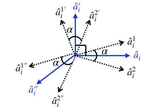
Figure 1: Directions chosen for pseudoprojections in construction of entanglement inequalities. $\hat{a}_{i},\hat{a}^{\prime}_{i},\hat{a}^{\prime\prime}_{i}$: Orthonormal triplets in the space of $i^{\rm th}$ qubit that appear in the entanglement inequality (shown in blue). $\hat{a}^{1,2}_{i},\hat{a}^{1^{\prime},2^{\prime}}_{i},\hat{a}^{1^{\prime\prime},2^{\prime\prime}}_{i}$: Directions used in the construction of pseudo-projection in the space of $i^{\rm th}$ qubit (shown in black).

Unlike in the case of nonlocality, we construct families of inequalities, some of which also involve higher order moments of pseudo probabilities. Separable states can also display non-classical features, e.g., quantum discord. Thus, in order to construct sufficiency conditions for entanglement, we explicitly preclude separable states by fixing the range of $\alpha$ in each case.

7.2 Linear entanglement inequalities: $N=3$

7.2.1 Inequality 1

The first set of events which we consider leads to entanglement inequalities involving only three body correlation terms. They involve the sum of pseudo probabilities,

$${\cal P}^{1}_{3}\equiv \sum_{i=1}^{2}\big{(}\mathcal{P}({\cal E}_{2}^{i};a^{\prime}_{3})+\mathcal{P}({\cal E}_{2}^{i+2};{\bar{a}}^{\prime}_{3})+\mathcal{P}({\cal E}_{2}^{i+4};a_{3})+\mathcal{P}({\cal E}_{2}^{i+6};{\bar{a}}_{3})\big{)},$$ (32)

where, ${\cal E}^{1}_{2}\equiv{\cal E}(a^{1}_{1}=a^{2}_{1}=a_{2});{\cal E}^{2}_{2}\equiv{\cal E}(a^{1^{\prime}}_{1}=a^{2^{\prime}}_{1}=a^{\prime}_{2})$. The other events are obtained via the transformations exhibited in Table (7).

Set of events	Observables
${\cal E}_{2}^{1,2}\rightarrow{\cal E}_{2}^{3,4}$ ${\cal E}_{2}^{5,6}\rightarrow{\cal E}_{2}^{7,8}$	$a_{2}(a^{\prime}_{2})\leftrightarrow{\bar{a}}_{2}({\bar{a}}^{\prime}_{2})$
${\cal E}_{2}^{1,2}\rightarrow{\cal E}_{2}^{5,6}$	$a_{2}\rightarrow a^{\prime}_{2};~{}a^{\prime}_{2}\rightarrow{\bar{a}}_{2}$ ${\bar{a}}_{2}\rightarrow{\bar{a}}^{\prime}_{2};~{}{\bar{a}}^{\prime}_{2}\rightarrow a_{2}$

Table 7: Transformation of ordered set of events and corresponding transformation of observables.

Writing the pseudoprobabilities and imposing the nonclassicality condition ${\cal P}_{3}^{1}<0,$ we arrive at the first family of entanglement inequalities

$$E^{1}_{3}\equiv\big{\langle} 4\cos\frac{\alpha}{2}+M_{3}\big{\rangle}<0;~{}0<\alpha\leq{\rm arccos}\Big{(}-\frac{7}{8}\Big{)},$$ (33)

where $M_{3}$ is the Mermin polynomial for the 3-qubit system. We now argue why the upper limit of $\alpha$ is ${\rm arccos}\Big{(}-\dfrac{7}{8}\Big{)}$. Note that $\langle M_{3}\rangle$ can take the minimum value $-1$ for separable states. To show this, without any loss of generality, we may choose:

$$a_{1}\equiv x_{1};~{}a^{\prime}_{1}\equiv y_{1};~{}a_{2}\equiv x_{2};~{}a^{\prime}_{2}\equiv y_{2};~{}a_{3}\equiv y_{3};~{}a^{\prime}_{3}\equiv x_{3}.$$

With this choice, $M_{3}$ takes the following form:

$$M_{3}\equiv(x_{1}x_{2}+y_{1}y_{2})x_{3}+(x_{1}y_{2}-y_{1}x_{2})y_{3},$$

whose minimum expectation value for a fully separable three-qubit pure state $\dfrac{1}{8}(1+p_{1})(1+p_{2})(1+p_{3})$ is $-1$. Since fully separable mixed states are convex sums of fully separable pure states, $\langle M_{3}\rangle$ has a lower bound of $-1$ for fully separable mixed states as well. Thus, if we demand that $\big{\langle}4\cos\dfrac{\alpha}{2}+M_{3}\big{\rangle}$ takes negative value only for entangled states, then $1\leq 4\cos\dfrac{\alpha}{2}<4$. This, in turn, fixes the range of $\alpha$ to be $0<\alpha\leq{\rm arccos}\Big{(}-\frac{7}{8}\Big{)}$. The bounds of $\alpha$ in the subsequent entanglement inequalities can be similarly found.

The detailed proof of inequality (33) is given in Appendix (D).

7.2.2 Inequality 2

We now refine the inequality $E^{1}_{3}$ (given in equation (33)) through the inclusion of two-body correlation terms. Of interest is the sum,

$${\cal P}^{2}_{3}\equiv {\cal P}^{1}_{3}+\sum_{(ij)}\mathcal{P}(a^{\prime\prime}_{i}=a_{j}^{1^{\prime\prime}}=a_{j}^{2^{\prime\prime}}).$$ (34)

Here $(ij)$ represents cyclic permutation of $i,j=1,2,3$. Writing the pseudoprobabilities and imposing the nonclassicality condition ${\cal P}^{2}_{3}<0$ implies the following inequality

$$E^{2}_{3}\equiv\big{\langle} 7\cos\dfrac{\alpha}{2}+M_{3}+a^{\prime\prime}_{1}a^{\prime\prime}_{2}+a^{\prime\prime}_{2}a^{\prime\prime}_{3}+a^{\prime\prime}_{3}a^{\prime\prime}_{1}\big{\rangle}<0;~{}0<\alpha\leq{\rm arccos}\Big{(}-\frac{31}{49}\Big{)}.$$ (35)

The range of $\alpha$ gets fixed by the demand that all the fully separable states violate the inequality $E_{3}^{2}$. The condition corresponding to $\alpha={\rm arccos}\big{(}-\frac{31}{49}\big{)}$ has been derived earlier as a $W$– witness by Acín et al.Acin01 using algebraic approaches.

7.2.3 Inequality 3

It is possible to derive new inequalities from this framework. For example, we introduce the following combination which involves the same pseudoprobabilities as in ${\cal P}^{2}_{3}$ but with different weights:

$${\cal P}^{3}_{3}\equiv {\cal P}^{1}_{3}+\dfrac{1}{3}\sum_{(ij)}\mathcal{P}(a^{\prime\prime}_{i}=a_{j}^{1^{\prime\prime}}=a_{j}^{2^{\prime\prime}}).$$ (36)

As before, writing the pseudoprobabilities and imposing the nonclassicality condition ${\cal P}^{3}_{3}<0$ yields the following inequality for inseparability:

$$E^{3}_{3}\equiv\Big{\langle}5\cos\dfrac{\alpha}{2}+M_{3}+ \frac{1}{3}\big{(}a^{\prime\prime}_{1}a^{\prime\prime}_{2}+a^{\prime\prime}_{2}a^{\prime\prime}_{3}+a^{\prime\prime}_{3}a^{\prime\prime}_{1}\big{)}\Big{\rangle}<0;~{}0<\alpha\leq{\rm arccos}\Big{(}-\frac{23}{25}\Big{)}.$$ (37)

The range of $\alpha$ gets fixed by the demand that all the completely separable states violate the inequality $E_{3}^{3}$. The detailed proof of inequality (37) is given in Appendix (E). Since the inequality is new, we also give the derivation for the range of $\alpha$ in the appendix.

The inequalities $E^{1}_{3},E^{2}_{3}$ and $E^{3}_{3}$ can also be be derived using stabiliser formalism, proposed in Toth05 . The present formalism successfully traces back the underlying cause to classical probability rule violations.

7.2.4 Inequality 4

Now we derive an entanglement inequality that involves correlation tensors as well as local terms for those three qubit states which are in the neighbourhood of the $W$-state. We start with the sum

$${\cal P}^{4}_{3}\equiv\ \sum_{i=1}^{3}{\cal P}(a^{1^{\prime\prime}}_{i},a^{2^{\prime\prime}}_{i})$$

$$+ \sum_{i<j=1}^{3}\Big{\{}{\cal P}(a^{1^{\prime\prime}}_{i}=a^{2^{\prime\prime}}_{i}={\bar{a}}^{\prime\prime}_{j})+2\big{\{}{\cal P}(a^{1^{\prime}}_{i}=a^{2^{\prime}}_{i}=a^{\prime}_{j})+{\cal P}(a^{1}_{i}=a^{2}_{i}=a_{j})\big{\}}\Big{\}}$$

$$+ 3\big{\{}{\cal P}(a^{1^{\prime\prime}}_{1}=a^{2^{\prime\prime}}_{1}=a^{\prime\prime}_{2};{\bar{a}}^{\prime\prime}_{3})+{\cal P}(a^{1^{\prime\prime}}_{1}=a^{2^{\prime\prime}}_{1}={\bar{a}}^{\prime\prime}_{2};a^{\prime\prime}_{3})\big{\}}$$

$$+ \sum_{(ijk)}\Big{\{}2\big{\{}\mathcal{P}(a^{1}_{i}=a^{2}_{i}=a_{j};a^{\prime\prime}_{k})+\mathcal{P}(a^{1^{\prime}}_{i}=a^{2^{\prime}}_{i}=a^{\prime}_{j};a^{\prime\prime}_{k})$$

$$+ \mathcal{P}(a^{1}_{i}=a^{2}_{i}={\bar{a}}_{j};{\bar{a}}^{\prime\prime}_{k})+\mathcal{P}(a^{1^{\prime}}_{i}=a^{2^{\prime}}_{i}={\bar{a}}^{\prime}_{j};{\bar{a}}^{\prime\prime}_{k})\big{\}}\Big{\}}.$$ (38)

Again, writing the pseudoprobabilities and imposing the nonclassicality condition the condition, ${\cal P}^{4}_{3}<0$, yields the following inequality for inseparability:

$$E^{4}_{3}\equiv\Big{\langle} 33\cos\dfrac{\alpha}{2}+\sum_{i=1}^{3}a^{\prime\prime}_{i}+\sum_{i<j=1}^{3}\{2(a_{i}a_{j}+a^{\prime}_{i}a^{\prime}_{j})-a^{\prime\prime}_{i}a^{\prime\prime}_{j}\}-3a^{\prime\prime}_{1}a^{\prime\prime}_{2}a^{\prime\prime}_{3}+$$

$$2\sum_{(ijk)}(a_{i}a_{j}+a^{\prime}_{i}a^{\prime}_{j})a^{\prime\prime}_{k}\Big{\rangle}<0,$$

$$0<\alpha\leq{\rm arccos}(-0.954)\approx\pi.$$ (39)

Here $(ijk)$ represents cyclic permutations of $i$, $j$ and $k$. The range of $\alpha$ gets fixed by the demand that all the completely separable states violate the inequality $E_{3}^{4}$. The inequality corresponding to one particular value, $\alpha={\rm arccos}(-0.689)$, was earlier derived in Acin01 as a $W$– witness.

7.3 Bilinear entanglement inequalities: $N=3$

So far we have considered violations of classical probability rules for linear combinations of pseudo-probabilities. We next turn our attention to combinations involving blinear terms in pseudo-probabilities.

7.3.1 Inequality 1

Consider, first, the sum of products of pseudoprobabilities:

$${\cal S}^{1}_{3}\equiv \Big{\{}\mathcal{P}({\cal E}_{2}^{1};a_{3})+\mathcal{P}({\cal E}_{2}^{2};a_{3})+\mathcal{P}({\cal E}_{2}^{3};{\bar{a}}_{3})+\mathcal{P}({\cal E}_{2}^{4};{\bar{a}}_{3})\Big{\}}$$

$$\times \Big{\{}\mathcal{P}({\cal E}_{2}^{1};{\bar{a}}_{3})+\mathcal{P}({\cal E}_{2}^{2};{\bar{a}}_{3})+\mathcal{P}({\cal E}_{2}^{3};a_{3})+\mathcal{P}({\cal E}_{2}^{4};a_{3})\Big{\}}$$

$$+ \big{\{}\mathcal{P}({\cal E}_{2}^{5};a^{\prime}_{3})+\mathcal{P}({\cal E}_{2}^{6};{\bar{a}}^{\prime}_{3})+\mathcal{P}({\cal E}_{2}^{7};{\bar{a}}^{\prime}_{3})+\mathcal{P}({\cal E}_{2}^{8};a^{\prime}_{3})\big{\}}$$

$$\times \big{\{}\mathcal{P}({\cal E}_{2}^{5};{\bar{a}}^{\prime}_{3})+\mathcal{P}({\cal E}_{2}^{6};a^{\prime}_{3})+\mathcal{P}({\cal E}_{2}^{7};a^{\prime}_{3})+\mathcal{P}({\cal E}_{2}^{8};{\bar{a}}^{\prime}_{3})\big{\}},$$ (40)

where, the events are given by,

$${\cal E}_{2}^{1}\equiv{\cal E}(a^{1}_{1}=a^{2}_{1}=a_{2});~{}{\cal E}_{2}^{2}\equiv{\cal E}(a^{1^{\prime}}_{1}=a^{2^{\prime}}_{1}=a^{\prime}_{2});$$

$${\cal E}_{2}^{3}\equiv{\cal E}(a^{1}_{1}=a^{2}_{1}={\bar{a}}_{2});~{}{\cal E}_{2}^{4}\equiv{\cal E}(a^{1^{\prime}}_{1}=a^{2^{\prime}}_{1}={\bar{a}}^{\prime}_{2})$$

$${\cal E}_{2}^{5}\equiv{\cal E}(a^{1}_{1}=a^{2}_{1}=a^{\prime}_{2});~{}{\cal E}_{2}^{6}\equiv{\cal E}(a^{1^{\prime}}_{1}=a^{2^{\prime}}_{1}=a_{2});$$

$${\cal E}_{2}^{7}\equiv{\cal E}(a^{1}_{1}=a^{2}_{1}={\bar{a}}^{\prime}_{2});~{}{\cal E}_{2}^{8}\equiv{\cal E}(a^{1^{\prime}}_{1}=a^{2^{\prime}}_{1}={\bar{a}}_{2}).$$ (41)

Writing the pseudoprobabilities and imposing the nonclassicality condition ${\cal S}^{1}_{3}<0$ yields the family of inequalities,

$$\mathbb{E}^{1}_{3}\equiv 8\cos^{2}\dfrac{\alpha}{2} -\big{\langle}(a_{1}a_{2}+a^{\prime}_{1}a^{\prime}_{2})a_{3}\big{\rangle}^{2}-\big{\langle}(a^{\prime}_{1}a_{2}-a_{1}a^{\prime}_{2})a^{\prime}_{3}\big{\rangle}^{2}<0$$

$$0<\alpha\leq{\rm arccos}\Big{(}-\frac{3}{4}\Big{)}$$ (42)

The range of $\alpha$ gets fixed by the demand that all the separable states violate the inequality $\mathbb{E}_{3}^{1}$.

7.3.2 Inequality 2

The second bilinear combination that we consider includes contribution from two-body correlation terms as well:

$${\cal S}^{2}_{3}\equiv \big{\{}\mathcal{P}({\cal E}_{2}^{1};a_{3})+\mathcal{P}({\cal E}_{2}^{3};{\bar{a}}_{3})\big{\}}\big{\{}\mathcal{P}({\cal E}_{2}^{1};{\bar{a}}_{3})+\mathcal{P}({\cal E}^{3};a_{3})\big{\}}$$

$$+ \big{\{}\mathcal{P}({\cal E}_{2}^{2};a_{3})+\mathcal{P}({\cal E}_{2}^{4};{\bar{a}}_{3})\big{\}}\big{\{}\mathcal{P}({\cal E}_{2}^{2};{\bar{a}}_{3})+\mathcal{P}({\cal E}^{4};a_{3})\big{\}}$$

$$+ \big{\{}\mathcal{P}({\cal E}_{2}^{5};a^{\prime}_{3})+\mathcal{P}({\cal E}_{2}^{7};{\bar{a}}^{\prime}_{3})\big{\}}\big{\{}\mathcal{P}({\cal E}_{2}^{5};{\bar{a}}^{\prime}_{3})+\mathcal{P}({\cal E}_{2}^{7};a^{\prime}_{3})\big{\}}$$

$$+ \big{\{}\mathcal{P}({\cal E}_{2}^{6};{\bar{a}}^{\prime}_{3})+\mathcal{P}({\cal E}_{2}^{6};a^{\prime}_{3})\big{\}}\big{\{}\mathcal{P}({\cal E}_{2}^{8};a^{\prime}_{3})+\mathcal{P}({\cal E}_{2}^{8};{\bar{a}}^{\prime}_{3})\big{\}}$$

$$+ \sum_{(ij)}\mathcal{P}(a^{\prime\prime}_{i}=a_{j}^{1^{\prime\prime}}=a_{j}^{2^{\prime\prime}})\mathcal{P}({\bar{a}}^{\prime\prime}_{i}=a_{j}^{1^{\prime\prime}}=a_{j}^{2^{\prime\prime}}),$$ (43)

where $\{{\cal E}_{2}^{1},\cdots,{\cal E}_{2}^{8}\}$ have been defined in equation (7.3.1). $(ij)$ represents cyclic permutations of $1,2,3$. Writing the pseudoprobabilities and imposing the nonclassicality condition ${\cal S}^{2}_{3}<0$ implies,

$$\mathbb{E}^{2}_{3} \equiv 7\cos^{2}\dfrac{\alpha}{2}-\langle a_{1}^{\prime\prime}a_{2}^{\prime\prime}\rangle^{2}-\langle a^{\prime\prime}_{2}a^{\prime\prime}_{3}\rangle^{2}-\langle a^{\prime\prime}_{3}a^{\prime\prime}_{1}\rangle^{2}$$

$$- \langle a_{1}a_{2}a_{3}\rangle^{2}-\langle a_{1}a^{\prime}_{2}a^{\prime}_{3}\rangle^{2}-\langle a^{\prime}_{1}a_{2}a^{\prime}_{3}\rangle^{2}-\langle a^{\prime}_{1}a^{\prime}_{2}a_{3}\rangle^{2}<0,$$

$$0<\alpha\leq{\rm arccos}\Big{(}-\frac{1}{7}\Big{)}.$$ (44)

The range of $\alpha$ gets fixed by the demand that all the fully separable states violate the inequality $\mathbb{E}_{3}^{2}$. The inequality corresponding to the particular value $\alpha={\rm arccos}\big{(}-\frac{1}{7}\big{)}$ has been derived in Guhne04 by invoking bounds on variances of observables for separable states vis-a vis fully tripartite entangled states.

7.4 Linear entanglement inequalities for $N$– qubit system

We now generalise our results by constructing an entanglement inequality involving $N$–body correlations. The correlation terms in the inequality are just the highest rank tensors that would occur in the $N$–qubit GHZ state. We start with the sum of pseudoprobabilities,

$${\cal P}_{N} =\sum_{i=1}^{\lambda}\big{\{}{\cal P}({\cal E}_{N-1}^{i};a^{\prime}_{N})+{\cal P}({\cal E}_{N-1}^{i+\lambda};{\bar{a}}^{\prime}_{N})+{\cal P}({\cal E}_{N-1}^{i+2\lambda};a_{N})+{\cal P}({\cal E}_{N-1}^{i+3\lambda};{\bar{a}}_{N})\big{\}};~{}N\geq 3.$$ (45)

where $\lambda=2^{2N-5}$ and the events ${\cal E}_{N-1}^{i};i\in\{1,\cdots,\lambda\}$ are to be extracted, recursively, from those pseudoprobabilities that underlie the entanglement inequality for $(N-1)$ qubits. The basic pseudo probabilities for two-qubits are given by

$${\cal P}_{2} ={\cal P}(a^{1}_{1}=a^{2}_{1}=a_{2})+{\cal P}(a^{1^{\prime}}_{1}=a^{2^{\prime}}_{1}=a^{\prime}_{2}).$$ (46)

Thus, ${\cal E}_{2}^{1}\equiv{\cal E}(a^{1}_{1}=a^{2}_{1}=a_{2})$ and ${\cal E}_{2}^{2}\equiv{\cal E}(a^{1^{\prime}}_{1}=a^{2^{\prime}}_{1}=a^{\prime}_{2})$.

Ordered set of events	Observables
$\{{\cal E}_{N-1}^{1},\cdots,{\cal E}_{N-1}^{\lambda}\}\rightarrow$ $\{{\cal E}_{N-1}^{\lambda+1},\cdots,{\cal E}_{N-1}^{2\lambda}\}$ $\{{\cal E}_{N-1}^{2\lambda+1},\cdots,{\cal E}_{N-1}^{3\lambda}\}\rightarrow$ $\{{\cal E}_{N-1}^{3\lambda+1},\cdots,{\cal E}_{N-1}^{4\lambda}\}$	$a_{N-1}\leftrightarrow{\bar{a}}_{N-1}$; $a^{\prime}_{N-1}\leftrightarrow{\bar{a}}^{\prime}_{N-1}$
$\{{\cal E}_{N-1}^{1},\cdots,{\cal E}_{N-1}^{\lambda}\}\rightarrow$	$a_{N-1}\rightarrow{a}^{\prime}_{N-1}$; $a^{\prime}_{N-1}\rightarrow{\bar{a}}_{N-1}$
$\{{\cal E}_{N-1}^{2\lambda+1},\cdots,{\cal E}_{N-1}^{3\lambda}\}$	${\bar{a}}_{N-1}\rightarrow{\bar{a}}^{\prime}_{N-1};~{}{\bar{a}}^{\prime}_{N-1}\rightarrow{a}_{N-1}$

Table 8: Transformation of ordered set of events and corresponding transformation of observables.

Writing all the pseudoprobabilites and imposing the nonclassicality condition ${\cal P}_{N}<0$, the entanglement inequality that follows has the form

$$E_{N}\equiv\Big{\langle}2^{N-1}\cos\dfrac{\alpha}{2}+M_{N}\Big{\rangle}<0,$$ (47)

Imposing the condition $E_{N}\geq 0$ for all the completely separable states fixes $0<\alpha\leq{\rm arccos}\Big{(}-\frac{2^{2N-3}-1}{2^{2N-3}}\Big{)}$, which approaches the value $\pi$ as $N\rightarrow\infty$. The range of $\alpha$ gets fixed by the demand that all the separable states violate the inequality $E_{N}$.

If $\alpha$ is left unrestricted, all the states with nonzero correlation tensor, i.e., having terms like $x_{1}x_{2}x_{3},x_{1}y_{2}y_{3},y_{1}x_{2}y_{3}$ and $y_{1}y_{2}x_{3}$ in the density matrix, will be detected to be nonclassical.

7.4.1 Comments on generalisation

It is by now clear that, by following the method that we have employed, numerous entanglement inequalities for a multi-party system can be constructed, by including correlations in the subsystems. The strength of the framework lies in the fact that no extra concept, other than violation of a classical probability rule, is required. The task gets further facilitated by a result which we prove in the Appendix (C): that any observable admits an expansion, with non-negative coefficients, in the overcomplete basis provided by a set of elementary pseudo projections. Specialisation to entanglement is accomplished by carving out suitable regions in the parameter space.

8 Examples

8.1 Three-qubit GHZ state with white noise

We now present the results for the noise resistance of the state, $|GHZ_{3}\rangle=\frac{1}{\sqrt{2}}(|000\rangle+|111\rangle$, with respect to the inequalities derived above. The state is given by

$$\rho_{p}=p|GHZ_{3}\rangle\langle GHZ_{3}|+(1-p)\frac{1}{8}I$$ (48)

where $I$ is the identity operator. The parameter $p$ determines the purity of the state. The ranges of $p$ for which $\rho_{p}$ is detected to be nonlocal or entangled by different nonlocality and entanglement inequalities are shown in tables (9) and (10) respectively.

Inequality	Range of $p$
${\cal I}_{S_{3}}$	$\frac{1}{\sqrt{2}}<p\leq 1$
${\cal I}_{M_{3}}$	$\frac{1}{2}<p\leq 1$

Table 9: Range of $p$ for which the state $\rho_{p}$ is detected to be nonlocal by Svetlichny and Mermin inequalities for hybrid local-nonlocal and completely factorisable local hidden variable models.

Inequality	Range of $p$
$E^{1}_{3}$	$\frac{1}{4}<p\leq 1$
$E^{2}_{3}$	$\frac{3}{5}<p\leq 1$
$E^{3}_{3}$	$\frac{1}{5}<p\leq 1$
$\mathbb{E}_{3}^{1}$	$\frac{1}{2\sqrt{2}}<p\leq 1$
$\mathbb{E}_{3}^{2}$	$\sqrt{\frac{3}{7}}<p\leq 1$

Table 10: Range of $p$ for which $\rho$ is detected to be entangled by different entanglement inequalities.

For graphical representation, we show the corresponding ranges of $p$ in figures (2) and (3) respectively. Evidently, the inequality $E^{3}_{3}$ detects the entangled states in the range $\dfrac{1}{5}<p\leq 1$. The entry in the fifth row, corresponding to $E^{3}_{3}$, has been obtained in Guhne10 by imposing conditions on the entries of density matrix of completely separable and entangled states using concavity arguments.

Figure 2: $AP$ and $AQ$: Ranges of $p$ for which the state $\rho$ is detected to be nonlocal by three-party Svetlichny and Mermin inequalities (${\cal I}_{S_{3}}$ and ${\cal I}_{M_{3}}$) respectively for hybrid local-nonlocal and completely factorisable local hidden variable models.

Figure 3: $AL_{1}$, $AL_{2}$, $AL_{3}$, $AL_{4}$, $AL_{5}$: Ranges of $p$ for which the state $\rho$ is detected to be entangled by entanglement inequalities $E_{3}^{3},E_{3}^{1},\mathbb{E}^{1}_{3},{E}^{2}_{3},\mathbb{E}^{2}_{3}$ respectively.

8.2 $N$-qubit GHZ state with white noise

The state $\rho_{p}=p|GHZ_{N}\rangle\langle GHZ_{N}|+\frac{1-p}{2^{N}}I$ is detected to be entangled by the inequality $E_{N}$ in the range $\frac{1}{2^{N-1}}<p\leq 1$.

9 Conclusion

In conclusion, we have proved that violation of any nonlocality inequality is equivalent to a sum of pseudoprobabilities assuming a negative value and any hermitian operator can be written as a sum of pseudoprojections with non-negative weights. The difference between both the features gets reflected in that the pseudoprobabilities in the former do not have their origin in any particular theory. Entanglement, being a nonclassical feature of quantum mechanics, the underlying pseudoprobabilities are expectations of pseudoprojections. Using this method, we have recovered a multitude of well known results for non locality and entanglement in multi party/multi qubit systems derived earlier by using several different means. Furthermore, we have derived a new family of entanglement inequalities in section (7.2.3). Finally, we have indicated how many more nonclassicality conditions may be derived without a need to introducing new concepts or techniques.

Author Contribution Statement

All the authors contributed equally in all respects.

Conflict of interest

The authors declare that they have no conflict of interest.

Appendix

Appendix A Violation of a nonlinear nonlocality inequality implies violation of a classical probability rule

In this appendix, we prove that violation of any nonlinear nonlocality inequality is equivalent to the nonexistence of an underlying nonnegative pseudoprobability scheme. We show it for a bipartite system, but the proof admits a straightforward generalisation to multipartite systems as well.

Condition for locality: Let $\{C_{\alpha}\}$ and $\{D_{\beta}\}$ be the sets of $N_{1}$ and $N_{2}$ observables for the first and the second subsystems of a bipartite system respectively. The respective sets of outcomes of the observables are $\{c^{i_{\alpha}}_{\alpha}\}$ and $\{d^{j_{\beta}}_{\beta}\}$. The most general nonlinear nonlocality inequality obeyed by all the local hidden variable models reads as,

$${\cal I}_{\rm NL}\equiv\sum_{abc\cdots}w_{abc\cdots}({\cal P}_{a})^{m_{a}}({\cal P}_{b})^{m_{b}}({\cal P}_{c})^{m_{c}}\cdots\leq R,$$ (49)

where all ${\cal P}_{a},{\cal P}_{b}$ and ${\cal P}_{c}$ are of the form ${\cal P}(C_{\alpha}=c^{i_{\alpha}}_{\alpha},D_{\beta}=d^{j_{\beta}}_{\beta})$, for some $(C_{\alpha},D_{\beta},c_{\alpha}^{i_{\alpha}},d_{\beta}^{j_{\beta}})$ and $m_{a},m_{b},m_{c},\cdots\geq 1$. The inequality has been so written that all $w_{abc\cdots}\geq 0$. All the inequalities can be brought in this form. For example, if there is a term ${\cal P}^{l}~{}(l>1),$ with a negative coefficient, then it can be rewritten as $1-{\cal P}^{\prime}(1+{\cal P}+{\cal P}^{2}+\cdots+{\cal P}^{l-1})$, where ${\cal P}^{\prime}$ is the probability of the complementary event.

Lemma: Let ${\cal M}_{1},{\cal M}_{2},\cdots$ be the sets of all the mutually consistent events $\{C_{\alpha}=c_{\alpha}^{i_{\alpha}},D_{\beta}=d_{\beta}^{j_{\beta}}\}$. For a given ${\cal M}_{k}$, let ${\cal N}_{k}$ represent the set of the coefficients $w_{abc\cdots}$ of those terms in inequality (49) that contain the probabilities for the mutually consistent events belonging to ${\cal M}_{k}$. If the sum of all $w_{abc\cdots}\in{\cal N}_{k}$ is represented by $R_{k}$, then,

$$R\geq\underset{\{{\cal N}_{k}\}}{\rm max}~{}R_{k},$$ (50)

where the maximum is taken over all ${\cal N}_{1},{\cal N}_{2},\cdots$.
Proof: For a given $k$, there always exists a local hidden variable model in which all the mutually consistent events belonging to the set ${\cal M}_{k}$ can be assigned unit probability (and all the other events inconsistent with the events belonging to ${\cal M}_{k}$ have zero probability). Since $k$ is an arbitrary label, equation (50) holds.

Theorem 1A: Violation of inequality (49) implies violation of a classical probability rule.
Proof: The proof follows from similar arguments as in section (4). Consider the expression,

$$R-{\cal I}_{\rm NL}=R-\sum_{abc\cdots}w_{abc\cdots}({\cal P}_{a})^{m_{a}}({\cal P}_{b})^{m_{b}}({\cal P}_{c})^{m_{c}}\cdots.$$ (51)

Since all the joint probabilities in the second term of equation (51) are of the form ${\cal P}(C_{\alpha}=c_{\alpha}^{i_{\alpha}},D_{\beta}=d_{\beta}^{j_{\beta}})$, we rewrite each of them as $\sideset{}{{}^{\prime}}{\sum}{\cal P}(\{C_{\alpha}=c_{\alpha}^{i_{\alpha}}\},\{D_{\beta}=d_{\beta}^{j_{\beta}}\})$, where $\sideset{}{{}^{\prime}}{\sum}$ represents summation over all the outcomes $\{c_{\alpha}^{i_{\alpha}}\}$ and $\{d_{\beta}^{j_{\beta}}\}$ except $c_{\alpha}^{i_{\alpha}}$ and $d_{\beta}^{j_{\beta}}$. Let ${\rm max}(m_{a}+m_{b}+m_{c}+\cdots)=M$, where the maximum is taken over all $a,b,c,\cdots$. Then, we insert the following identity in the first term of equation (51):

$$\Big{\{}\sum_{\begin{subarray}{c}i_{1}\cdots i_{N_{1}}\\ j_{1}\cdots j_{N_{2}}\end{subarray}}{\cal P}(\{C_{\alpha}=c_{\alpha}^{i_{\alpha}}\},\{D_{\beta}=d_{\beta}^{j_{\beta}}\})\Big{\}}^{M}=1.$$ (52)

It is straightforward to see that the coefficients of all the joint probabilities of all orders in eqaution (51), after these substitutions, are nonnegative. If, in addition, the joint probabilities are also nonnegative, it follows that,

$$R-{\cal I}_{\rm NL}\geq 0\implies{\cal I}_{\rm NL}\leq R,$$ (53)

which agrees with the locality condition given in equation (49). Thus, in order that the locality condition gets violated, some of the joint probabilities have to turn negative. This implies that in place of a joint probabilities, we have pseudoprobabilities that may assume negative values as well.

Appendix B Derivation of the three-party Svetlichny inequality

In this section, we detail the derivation of the three-party Svetlichny inequality. First, we write the joint probabilities of the events in terms of expectation values as follows:

$${\cal E}_{2}^{\alpha} \equiv{\cal E}({\bar{A}}_{1}=A^{\prime}_{1}=A_{2})\vee{\cal E}(A_{1}=A^{\prime}_{1}=A^{\prime}_{2})$$

$$\equiv{\cal E}({\bar{A}}_{1}A^{\prime}_{1};A_{2})\vee{\cal E}(A_{1}{\bar{A}}^{\prime}_{1};{\bar{A}}_{2})\vee{\cal E}(A_{1}A^{\prime}_{1};A^{\prime}_{2})\vee{\cal E}({\bar{A}}_{1}{\bar{A}}^{\prime}_{1};{\bar{A}}^{\prime}_{2})$$

$${\cal P}({\cal E}^{\alpha}_{2};A^{\prime}_{3}) =\dfrac{1}{16}\Big{\langle}\Big{\{}(1-A_{1}A^{\prime}_{1}+(-A_{1}+A^{\prime}_{1})A_{2}-A_{1}+A^{\prime}_{1}+A_{2})\Big{\}}$$

$$+(1-A_{1}A^{\prime}_{1}+(-A_{1}+A^{\prime}_{1})A_{2}+A_{1}-A^{\prime}_{1}-A_{2})$$

$$+(1+A_{1}A^{\prime}_{1}+(A_{1}+A^{\prime}_{1})A^{\prime}_{2}+A_{1}+A^{\prime}_{1}+A^{\prime}_{2})$$

$$+(1+A_{1}A^{\prime}_{1}+(A_{1}+A^{\prime}_{1})A^{\prime}_{2}-A_{1}-A^{\prime}_{1}-A^{\prime}_{2})\Big{\}}(1+A^{\prime}_{3})\Big{\rangle}$$

$$=\dfrac{1}{8}\Big{\langle}\Big{\{}2+(-A_{1}+A^{\prime}_{1})A_{2}+(A_{1}+A^{\prime}_{1})A^{\prime}_{2}\Big{\}}(1+A^{\prime}_{3})\Big{\rangle}$$

Thus,

$${\cal P}({\cal E}^{\alpha}_{2};A^{\prime}_{3})+{\cal P}({\cal E}^{\alpha^{\prime}}_{2};{\bar{A}}^{\prime}_{3}) =\dfrac{1}{4}\Big{\langle}\Big{\{}2+\{(-A_{1}+A^{\prime}_{1})A_{2}+(A_{1}+A^{\prime}_{1})A^{\prime}_{2}\}A^{\prime}_{3}\Big{\}}\Big{\rangle}$$ (54)

Similarly,

$${\cal P}({\cal E}^{\beta}_{2};A_{3})+{\cal P}({\cal E}^{\beta^{\prime}}_{2};{\bar{A}}_{3}) =\dfrac{1}{4}\Big{\langle}\Big{\{}2+\{(-A^{\prime}_{1}+A_{1})A^{\prime}_{2}+(A_{1}+A^{\prime}_{1})A_{2}\}A_{3}\Big{\}}\Big{\rangle}$$ (55)

Adding the joint probabilities in equations (54) and (55),

$${\cal P}^{S}_{3}\equiv {\cal P}({\cal E}^{\alpha}_{2};A^{\prime}_{3})+{\cal P}({\cal E}^{\alpha^{\prime}}_{2};{\bar{A}}^{\prime}_{3})+{\cal P}({\cal E}^{\beta}_{2};A_{3})+{\cal P}({\cal E}^{\beta^{\prime}}_{2};{\bar{A}}_{3})$$

$$=\dfrac{1}{4}\Big{\langle} \big{\{}4+\{(-A_{1}+A^{\prime}_{1})A_{2}+(A_{1}+A^{\prime}_{1})A^{\prime}_{2}\}A^{\prime}_{3}+\{(-A^{\prime}_{1}+A_{1})A^{\prime}_{2}+(A_{1}+A^{\prime}_{1})A_{2}\}A_{3}\big{\}}\Big{\rangle}$$ (56)

Imposing the demand ${\cal P}^{S}_{3}<0$, the following inequality emerges

$$\langle S_{3}\rangle<-4.$$ (57)

Interchanging ${\bar{A}}_{1}$ and ${\bar{A}}^{\prime}_{1}$ with ${A}_{1}$ and ${A}^{\prime}_{1}$ respectively in equation (B) and imposing the nonclassicality condition, we obtain the complementary condition $\langle S_{3}\rangle>4$, which, together with the condition given in equation (57) yields $|\langle S_{3}\rangle|>4$.

Appendix C Expansion of any hermitian operator as sum of pseudoprojections

In this appendix, we show how an arbitrary hermitian operator $\hat{O}$ in dimension $d$ can be expanded as sum of pseudoprojections with non-negative weights. Let the hermitian operator $\hat{O}$ be written in the basis spanned by generalised Pauli matrices as:

$$\hat{O}= w+x^{ij}X_{ij}+y^{ij}Y_{ij}+z^{l}Z_{l}$$

$$= w+(x_{+}^{ij}+x_{-}^{ij})X_{ij}+(y_{+}^{ij}+y_{-}^{ij})Y_{ij}+(z_{+}^{l}+z_{-}^{l})Z_{l}$$

$$= w+(x_{+}^{ij}+x^{ij}_{-})X_{ij}+(y^{ij}_{+}+y^{ij}_{-})Y_{ij}+(z^{i,l+1}_{+}+z^{i,l+1}_{-})Z_{i,l+1}$$ (58)

where,

$$f^{ij}_{\pm}=f^{ij}\Theta(\pm f^{ij}).$$ (59)

$\Theta(\cdot)$ represents Heaviside unit step function. Repeated indices are all summed over and,

$$X_{ij}^{kl}= \delta_{ki}\delta_{lj}+\delta_{li}\delta_{kj}~{}{\rm for}~{}1\leq i<j\leq d,$$

$$Y_{ij}^{kl}= -i(\delta_{ki}\delta_{lj}-\delta_{li}\delta_{kj})~{}{\rm for}~{}1\leq i<j\leq d,$$

$$Z_{l}= \sqrt{\frac{2}{l(l+1)}}\Big{(}\sum_{j=1}^{l}|j\rangle\langle j|-l|l+1\rangle\langle l+1|\Big{)};~{}1\leq~{}l~{}\leq~{}d-1,$$

$$= \sqrt{\frac{2}{l(l+1)}}\Big{\{}(|1\rangle\langle 1|-|l+1\rangle\langle l+1|)+\cdots+(|l\rangle\langle l|-|l+1\rangle\langle l+1|)\Big{\}}$$

$$= \sqrt{\frac{2}{l(l+1)}}\Big{\{}Z_{1,l+1}+\cdots+Z_{l,l+1}\Big{\}}.$$ (60)

where

$$Z_{i,l+1}=|i\rangle\langle i|-|l+1\rangle\langle l+1|;~{}i=1,\cdots,l$$

We introduce two doublets of unit vectors ($\hat{p}_{1}$, $\hat{p}_{2}$) and ($\hat{q}_{1}$, $\hat{q}_{2}$) such that the included angle between the two vectors of each doublet is $\theta$. Let $(\hat{p}_{1}+\hat{p}_{2}),(\hat{p}_{1}-\hat{p}_{2})$ and $(\hat{q}_{1}+\hat{q}_{2})$ form an orthonormal triad, then we can always choose $(\hat{p}_{1}+\hat{p}_{2})\parallel\hat{x}$, $(\hat{p}_{1}-\hat{p}_{2})\parallel\hat{y}$, $(\hat{q}_{1}+\hat{q}_{2})\parallel\hat{z}$. Following are the short-hand notations for pseudoprojections for different joint events:

$${\bf\Pi}_{p^{ij}_{1}p^{ij}_{2}}\equiv{\bf\Pi}^{X_{ij}}_{+};~{}~{}~{}~{}{\bf\Pi}_{{\bar{p}}^{ij}_{1}{\bar{p}}^{ij}_{2}}\equiv{\bf\Pi}^{X_{ij}}_{-}$$

$${\bf\Pi}_{{p}^{ij}_{1}{\bar{p}}^{ij}_{2}}\equiv{\bf\Pi}^{Y_{ij}}_{+};~{}~{}~{}~{}{\bf\Pi}_{{\bar{p}}^{ij}_{1}p^{ij}_{2}}\equiv{\bf\Pi}^{Y_{ij}}_{-}$$

$${\bf\Pi}_{q^{ij}_{1}q^{ij}_{2}}\equiv{\bf\Pi}^{Z_{ij}}_{+};~{}~{}~{}~{}{\bf\Pi}_{{\bar{q}}^{ij}_{1}{\bar{q}}^{ij}_{2}}\equiv{\bf\Pi}^{Z_{ij}}_{-},$$ (61)

Here $p_{1}^{ij}\equiv\vec{\sigma}^{ij}\cdot\hat{p}_{1}$ and so on.

One more pseudoprojection ${\bf\Pi}_{r^{ij}_{1}r^{ij}_{2}r^{ij}_{3}}$, representing the joint event $\vec{\sigma}_{ij}\cdot\hat{r}_{1}=+1;~{}\vec{\sigma}_{ij}\cdot\hat{r}_{2}=+1;~{}\vec{\sigma}_{ij}\cdot\hat{r}_{3}=+1$, will also be required; where $\hat{r}_{i}$ are coplanar and at an included angle of $2\pi/3$ with each other,

$${\bf\Pi}_{r^{ij}_{1}r^{ij}_{2}r^{ij}_{3}} =\dfrac{1}{3!}\big{(}\pi_{r^{ij}_{1}}\pi_{r^{ij}_{2}}\pi_{r^{ij}_{3}}+\pi_{r^{ij}_{1}}\pi_{r^{ij}_{3}}\pi_{r^{ij}_{2}}+\pi_{r^{ij}_{2}}\pi_{r^{ij}_{1}}\pi_{r^{ij}_{3}}+\pi_{r^{ij}_{2}}\pi_{r^{ij}_{3}}\pi_{r^{ij}_{1}}$$

$$+\pi_{r^{ij}_{3}}\pi_{r^{ij}_{1}}\pi_{r^{ij}_{2}}+\pi_{r^{ij}_{3}}\pi_{r^{ij}_{2}}\pi_{r^{ij}_{1}}\big{)}=-1_{ij}/16,$$

where $1_{ij}^{kl}=\delta_{ik}\delta_{il}+\delta_{jk}\delta_{jl}$.
The expressions of different pseudoprojections are as follows:

$${\bf\Pi}_{\pm}^{X_{ij}}=\dfrac{1}{2}\cos\dfrac{\theta}{2}\Big{(}\cos\dfrac{\theta}{2}1_{ij}\pm X_{ij}\Big{)};~{}~{}{\bf\Pi}_{\pm}^{Y_{ij}}=\dfrac{1}{2}\sin\dfrac{\theta}{2}\Big{(}\sin\dfrac{\theta}{2}1_{ij}\pm Y_{ij}\Big{)}$$

$${\bf\Pi}^{Z_{i,l+1}}_{\pm}=\dfrac{1}{2}\cos\dfrac{\theta}{2}\Big{(}\cos\dfrac{\theta}{2}1_{i,l+1}\pm Z_{i,l+1}\Big{)}.$$ (62)

The operator $\hat{O}$ can be expanded in terms of pseudoprojections and the expansion coefficients are as follows:

$$\hat{O}= c+2\sec\frac{\theta}{2}\Big{(}x^{ij}_{+}{\bf\Pi}^{X_{ij}}_{+}+|x^{ij}_{-}|{\bf\Pi}^{X_{ij}}_{-}+z^{{}^{\prime}i,l+1}_{+}{\bf\Pi}^{Z_{i,l+1}}_{+}+|z^{{}^{\prime}i,l+1}_{-}|{\bf\Pi}^{Z_{i,l+1}}_{-}\Big{)}$$

$$+ 2{\rm cosec}\frac{\theta}{2}\Big{(}y^{ij}_{+}{\bf\Pi}^{Y_{ij}}_{+}+|y^{ij}_{-}|{\bf\Pi}^{Y_{ij}}_{-}\Big{)}$$ (63)

where

$$z^{{}^{\prime}}_{+} =\sqrt{\frac{2}{l(l+1)}}z_{+};z^{{}^{\prime}}_{-}=\sqrt{\frac{2}{l(l+1)}}z_{-},$$

$$c= \Big{\{}w-(x_{+}^{ij}+|x_{-}^{ij}|)\cos\frac{\theta}{2}1_{ij}-(y_{+}^{ij}+|y_{-}^{ij}|)\sin\frac{\theta}{2}1_{ij}-(z^{{}^{\prime}i,l+1}_{+}+|z^{{}^{\prime}i,l+1}_{-}|)\cos\frac{\theta}{2}1_{i,l+1}\Big{\}}$$

$$= \Big{\{}\frac{w}{d-1}\sum_{i<j=1}^{d}\Big{(}\sec^{2}\frac{\theta}{2}({\bf\Pi}^{X_{ij}}_{+}+{\bf\Pi}^{X_{ij}}_{-})\Theta(w)+16{\bf\Pi}_{r^{ij}_{1}r^{ij}_{2}r^{ij}_{3}}\Theta(-w)\Big{)}+$$

$$+ 16\Big{(}(x_{+}^{ij}+|x^{ij}_{-}|)\cos\frac{\theta}{2}+(y_{+}^{ij}+|y^{ij}_{-}|)\sin\frac{\theta}{2}\Big{)}{\bf\Pi}_{r^{ij}_{1}r^{ij}_{2}r^{ij}_{3}}$$

$$+ 16(z^{{}^{\prime}i,l+1}_{+}+|z^{{}^{\prime}i,l+1}_{-}|)\cos\frac{\theta}{2}{\bf\Pi}_{r_{1}^{i,l+1}r_{2}^{i,l+1}r_{3}^{i,l+1}}\Big{\}}$$ (64)

Here, $\Theta(w)$ represents Heaviside step function.

Appendix D Derivation of the entanglement inequality $E_{3}^{1}$

The sum of pseudoprobabilities underlying this inequality is given in equation (32), which is as follows:

$${\cal P}^{1}_{3}\equiv \sum_{i=1}^{2}\big{(}\mathcal{P}({\cal E}_{2}^{i};a^{\prime}_{3})+\mathcal{P}({\cal E}_{2}^{i+2};{\bar{a}}^{\prime}_{3})+\mathcal{P}({\cal E}_{2}^{i+4};a_{3})+\mathcal{P}({\cal E}_{2}^{i+6};{\bar{a}}_{3})\big{)},$$ (65)

where, ${\cal E}^{1}_{2}\equiv{\cal E}(a^{1}_{1}=a^{2}_{1}=a_{2});{\cal E}^{2}_{2}\equiv{\cal E}(a^{1^{\prime}}_{1}=a^{2^{\prime}}_{1}=a^{\prime}_{2})$. The psudoprobabilities corresponding to different events in equation (32) are as follows

$${\cal P}({\cal E}^{1}_{2})={\cal P}(a^{1}_{1}=a^{2}_{1}=a_{2}) =\Big{\langle}\dfrac{1}{4}\cos\dfrac{\alpha}{2}\Big{(}\cos\dfrac{\alpha}{2}+a_{1}\Big{)}(1+a_{2})+\dfrac{1}{4}\cos\dfrac{\alpha}{2}\Big{(}\cos\dfrac{\alpha}{2}-a_{1}\Big{)}(1-a_{2})\Big{\rangle}$$

$$=\Big{\langle}\dfrac{1}{4}\cos\dfrac{\alpha}{2}\Big{(}2\cos\dfrac{\alpha}{2}+2a_{1}a_{2}\Big{)}\Big{\rangle}$$ (66)

Similarly,

$${\cal P}({\cal E}_{2}^{2}) =\Big{\langle}\dfrac{1}{4}\cos\dfrac{\alpha}{2}\Big{(}2\cos\dfrac{\alpha}{2}+2a^{\prime}_{1}a^{\prime}_{2}\Big{)}\Big{\rangle}$$

$${\cal P}({\cal E}_{2}^{3}) =\Big{\langle}\dfrac{1}{4}\cos\dfrac{\alpha}{2}\Big{(}2\cos\dfrac{\alpha}{2}-2a_{1}a_{2}\Big{)}\Big{\rangle};~{}~{}~{}{\cal P}({\cal E}_{2}^{4}) =\Big{\langle}\dfrac{1}{4}\cos\dfrac{\alpha}{2}\Big{(}2\cos\dfrac{\alpha}{2}-2a^{\prime}_{1}a^{\prime}_{2}\Big{)}\Big{\rangle}$$

$${\cal P}({\cal E}_{2}^{5}) =\Big{\langle}\dfrac{1}{4}\cos\dfrac{\alpha}{2}\Big{(}2\cos\dfrac{\alpha}{2}+2a_{1}a^{\prime}_{2}\Big{)}\Big{\rangle};~{}~{}~{}{\cal P}({\cal E}_{2}^{6}) =\Big{\langle}\dfrac{1}{4}\cos\dfrac{\alpha}{2}\Big{(}2\cos\dfrac{\alpha}{2}-2a^{\prime}_{1}a_{2}\Big{)}\Big{\rangle}$$

$${\cal P}({\cal E}_{2}^{7}) =\Big{\langle}\dfrac{1}{4}\cos\dfrac{\alpha}{2}\Big{(}2\cos\dfrac{\alpha}{2}-2a_{1}a^{\prime}_{2}\Big{)}\Big{\rangle};~{}~{}~{}{\cal P}({\cal E}_{2}^{8}) =\Big{\langle}\dfrac{1}{4}\cos\dfrac{\alpha}{2}\Big{(}2\cos\dfrac{\alpha}{2}+2a^{\prime}_{1}a_{2}\Big{)}\Big{\rangle}$$ (67)

Substituting these explicit forms of the pseudoprobabilities in eqaution (33), we obtain

$${\cal P}({\cal E}_{2}^{1};a_{3}^{\prime})+{\cal P}({\cal E}_{2}^{2};a_{3}^{\prime})+{\cal P}({\cal E}_{2}^{3};{\bar{a}}_{3}^{\prime})+{\cal P}({\cal E}_{2}^{4};{\bar{a}}_{3}^{\prime})+$$

$${\cal P}({\cal E}_{2}^{5};a_{3})+{\cal P}({\cal E}_{2}^{6};a_{3})+{\cal P}({\cal E}_{2}^{7};{\bar{a}}_{3})+{\cal P}({\cal E}_{2}^{8};{\bar{a}}_{3})$$

$$= \dfrac{1}{4}\cos\dfrac{\alpha}{2}\Big{\langle}\Big{[}\Big{\{}\Big{(}\cos\dfrac{\alpha}{2}+a_{1}a_{2}\Big{)}+\Big{(}\cos\dfrac{\alpha}{2}+a^{\prime}_{1}a^{\prime}_{2}\Big{)}\Big{\}}(1+a^{\prime}_{3})$$

$$+ \Big{\{}\Big{(}\cos\dfrac{\alpha}{2}-a_{1}a_{2}\Big{)}+\Big{(}\cos\dfrac{\alpha}{2}-a^{\prime}_{1}a^{\prime}_{2}\Big{)}\Big{\}}(1-a^{\prime}_{3})$$

$$+ \Big{\{}\Big{(}\cos\dfrac{\alpha}{2}+a_{1}a^{\prime}_{2}\Big{)}+\Big{(}\cos\dfrac{\alpha}{2}-a^{\prime}_{1}a_{2}\Big{)}\Big{\}}(1+a_{3})$$

$$+ \Big{\{}\Big{(}\cos\dfrac{\alpha}{2}-a_{1}a^{\prime}_{2}\Big{)}+\Big{(}\cos\dfrac{\alpha}{2}+a^{\prime}_{1}a^{\prime}_{2}\Big{)}\Big{\}}(1-a_{3})\Big{\}}\Big{]}\Big{\rangle}$$

$$= \dfrac{1}{4}\cos\dfrac{\alpha}{2}\Big{\langle}8\cos\dfrac{\alpha}{2}+2(a_{1}a_{2}+a^{\prime}_{1}a^{\prime}_{2})a^{\prime}_{3}+2(a_{1}a^{\prime}_{2}-a^{\prime}_{1}a_{2})a_{3}\Big{\rangle}$$ (68)

Imposing the nonclassicality condition on equation (68), i.e., demanding the sum of pseudoprobabilities to be negative, the inequality $E_{3}^{1}$ emerges.

Appendix E Proof of the entanglement inequality $E_{3}^{3}$

We have the following relation:

$${\cal P}(a_{i}{{}^{\prime\prime}}=a_{j}^{1^{\prime\prime}}=a_{j}^{2^{\prime\prime}})= {\cal P}(a_{i}{{}^{\prime\prime}}=a_{j}^{1^{\prime\prime}}=a_{j}^{2^{\prime\prime}}=+1)+{\cal P}(a_{i}{{}^{\prime\prime}}=a_{j}^{1^{\prime\prime}}=a_{j}^{2^{\prime\prime}}=-1)$$

$$= \dfrac{1}{4}\cos\dfrac{\alpha}{2}\Big{\langle}\Big{(}\cos\dfrac{\alpha}{2}+a_{i}^{\prime\prime}\Big{)}\Big{(}1+a_{j}^{\prime\prime}\Big{)}+\Big{(}\cos\dfrac{\alpha}{2}-a_{i}^{\prime\prime}\Big{)}\Big{(}1-a_{j}^{\prime\prime}\Big{)}\Big{\rangle}$$

$$= \dfrac{1}{4}\cos\dfrac{\alpha}{2}\Big{(}2\cos\dfrac{\alpha}{2}+2a^{\prime\prime}_{i}a^{\prime\prime}_{j}\Big{)}\Big{\rangle}=\dfrac{1}{2}\cos\dfrac{\alpha}{2}\Big{(}\cos\dfrac{\alpha}{2}+a^{\prime\prime}_{i}a^{\prime\prime}_{j}\Big{)}\Big{\rangle}$$ (69)

Thus, plugging the values from equations (68) and (69),

$${\cal P}({\cal E}_{2}^{1};a_{3}^{\prime})+{\cal P}({\cal E}_{2}^{2};a_{3}^{\prime})+{\cal P}({\cal E}_{2}^{3};{\bar{a}}_{3}^{\prime})+{\cal P}({\cal E}_{2}^{4};{\bar{a}}_{3}^{\prime})$$

$$+ {\cal P}({\cal E}_{2}^{5};a_{3})+{\cal P}({\cal E}_{2}^{6};a_{3})+{\cal P}({\cal E}_{2}^{7};{\bar{a}}_{3})+{\cal P}({\cal E}_{2}^{8};{\bar{a}}_{3})+\frac{1}{3}\sum_{(ij)}{\cal P}(a^{\prime\prime}_{i}=a^{1^{\prime\prime}}_{j}=a^{2^{\prime\prime}}_{j})$$

$$= \dfrac{1}{2}\cos\dfrac{\alpha}{2}\Big{\langle}5\cos\dfrac{\alpha}{2}+M_{3}+\dfrac{1}{3}(a^{\prime\prime}_{1}a^{\prime\prime}_{2}+a^{\prime\prime}_{2}a^{\prime\prime}_{3}+a^{\prime\prime}_{3}a^{\prime\prime}_{1})\Big{\rangle}$$ (70)

Imposing the nonclassicality condition on equation (70), i.e., demanding the sum of pseudoprobabilities to be negative, the inequality $E_{3}^{3}$ emerges, i.e.,

$$\Big{\langle}5\cos\dfrac{\alpha}{2}+M_{3}+\dfrac{1}{3}(a^{\prime\prime}_{1}a^{\prime\prime}_{2}+a^{\prime\prime}_{2}a^{\prime\prime}_{3}+a^{\prime\prime}_{3}a^{\prime\prime}_{1})\Big{\rangle}<0$$

In order to fix the range of $\alpha$, note that, without any loss of generality, we may choose,

$$a_{1}\equiv x_{1};~{}a^{\prime}_{1}\equiv y_{1};~{}a^{\prime\prime}_{1}\equiv z_{1};~{}a_{2}\equiv x_{2};~{}a^{\prime}_{2}\equiv y_{2};~{}a^{\prime\prime}_{2}\equiv z_{2};~{}a_{3}\equiv y_{3};~{}a^{\prime}_{3}\equiv x_{3};a^{\prime\prime}_{3}\equiv z_{3}.$$

With this choice,

$$M_{3}+\dfrac{1}{3}(a^{\prime\prime}_{1}a^{\prime\prime}_{2}+a^{\prime\prime}_{2}a^{\prime\prime}_{3}+a^{\prime\prime}_{3}a^{\prime\prime}_{1}) \equiv(x_{1}x_{2}+y_{1}y_{2})x_{3}+(x_{1}y_{2}-y_{1}x_{2})y_{3}$$

$$+\dfrac{1}{3}(z_{1}z_{2}+z_{2}z_{3}+z_{3}z_{1}),$$

whose expectation value for a pure separable three -qubit state $\frac{1}{8}(1+p_{1})(1+p_{2})(1+p_{3})$ ($|p_{1}|=|p_{2}|=|p_{3}|=1$) is given by,

$$(p_{1x}p_{2x}+p_{1y}p_{2y})p_{3x}+(p_{1x}p_{2y}-p_{1y}p_{2x})p_{3y}+\dfrac{1}{3}(p_{1z}p_{2z}+p_{2z}p_{3z}+p_{3z}p_{1z}).$$ (71)

If $\vec{p}_{i}\equiv(p_{ix},p_{iy},p_{iz})\equiv(\sin\theta_{i}\cos\phi_{i},\sin\theta_{i}\sin\phi_{i},\cos\theta_{i});i\in\{1,2,3\}$, then,

$$(p_{1x}p_{2x}+p_{1y}p_{2y})p_{3x}+(p_{1x}p_{2y}-p_{1y}p_{2x})p_{3y}+\dfrac{1}{3}(p_{1z}p_{2z}+p_{2z}p_{3z}+p_{3z}p_{1z})$$

$$= \sin\theta_{1}\sin\theta_{2}\sin\theta_{3}\cos(\phi_{1}-\phi_{2}+\phi_{3})+\dfrac{1}{3}(\cos\theta_{1}\cos\theta_{2}+\cos\theta_{2}\cos\theta_{3}+\cos\theta_{3}\cos\theta_{1})$$

$$\geq -\sin\theta_{1}\sin\theta_{2}\sin\theta_{3}+\dfrac{1}{3}(\cos\theta_{1}\cos\theta_{2}+\cos\theta_{2}\cos\theta_{3}+\cos\theta_{3}\cos\theta_{1})$$

$$= \dfrac{1}{3}\big{(}-3\sin\theta_{1}\sin\theta_{2}\sin\theta_{3}+\cos\theta_{1}\cos\theta_{2}+\cos\theta_{2}\cos\theta_{3}+\cos\theta_{3}\cos\theta_{1}\big{)}$$

$$\geq \dfrac{1}{3}\big{(}\cos(\theta_{1}+\theta_{2})+\cos(\theta_{2}+\theta_{3})+\cos(\theta_{3}+\theta_{1})\big{)}\geq-1.$$ (72)

Thus, in order that the inequality $\Big{\langle}5\cos\alpha+M_{3}+\dfrac{1}{3}(a^{\prime\prime}_{1}a^{\prime\prime}_{2}+a^{\prime\prime}_{2}a^{\prime\prime}_{3}+a^{\prime\prime}_{3}a^{\prime\prime}_{1})\Big{\rangle}<0$ gets violated by all separable states, $1\leq 5\cos\dfrac{\alpha}{2}<5$, which, in turn fixes the range of $\alpha$ to be $0<\alpha\leq{\rm arccos}\Big{(}-\dfrac{23}{25}\Big{)}$.

References

• (1) J.F. Clauser, M.A. Horne, A. Shimony, R.A. Holt, Phys. Rev. Lett. 23(15), 880 (October 1969)
• (2) J.S. Bell, Physics 1, 195 (1964)
• (3) C.H. Bennett, G. Brassard, C. Crépeau, R. Jozsa, A. Peres, W.K. Wootters, Phys. Rev. Lett. 70, 1895 (1993). DOI 10.1103/PhysRevLett.70.1895
• (4) A.K. Ekert, Phys. Rev. Lett. 67, 661 (1991). DOI 10.1103/PhysRevLett.67.661. URL https://link.aps.org/doi/10.1103/PhysRevLett.67.661
• (5) D. Deutsch, Proceedings of the Royal Society of London. Series A, Mathematical and Physical Sciences 400(1818), 97 (1985). DOI 10.2307/2397601
• (6) J. Bouda, V. Buzek, Journal of Physics A: Mathematical and General 34(20), 4301 (2001)
• (7) W. Jian, Z. Quan, T. Chao-Jing, Communications in Theoretical Physics 48(4), 637 (2007)
• (8) M. Epping, H. Kampermann, C. macchiavello, D. Bruß, New Journal of Physics 19(9), 093012 (2017)
• (9) G. Svetlichny, Phys. Rev. D 35, 3066 (1987)
• (10) R. Horodecki, P. Horodecki, M. Horodecki, K. Horodecki, Rev. Mod. Phys. 81, 865 (2009)
• (11) H. Ollivier, W.H. Zurek, Phys. Rev. Lett. 88, 017901 (2001)
• (12) N.D. Mermin, Phys. Rev. Lett. 65, 1838 (1990)
• (13) A. Acín, D. Bruß, M. Lewenstein, A. Sanpera, Phys. Rev. Lett. 87, 040401 (2001)
• (14) M. Seevinck, G. Svetlichny, Phys. Rev. Lett. 89, 060401 (2002)
• (15) G. Tóth, O. Gühne, Phys. Rev. A 72, 022340 (2005)
• (16) O. Gühne, M. Seevinck, New Journal of Physics 12(5), 053002 (2010)
• (17) J.I. de Vicente, M. Huber, Phys. Rev. A 84, 062306 (2011)
• (18) P.A.M. Dirac, Proceedings of the Royal Society of London A: Mathematical, Physical and Engineering Sciences 180(980), 1 (1942)
• (19) M.S. Bartlett, Mathematical Proceedings of the Cambridge Philosophical Society 41(1), 71–73 (1945). DOI 10.1017/S0305004100022398
• (20) R.P. Feynman, Chapter- 13, Quantum implications: essays in honour of David Bohm (edited by B. Hiley and F. Peat)
• (21) A. Fine, Phys. Rev. Lett. 48, 291 (1982)
• (22) S. Adhikary, S. Asthana, V. Ravishankar, Eur. Phys. J. D 74(68), 68 (2020)
• (23) H. Margenau, R.N. Hill, Progress of Theoretical Physics 26(5), 722 (1961)
• (24) A.O. Barut, M. Božić, Z. Marić, Foundations of Physics 18(10), 999 (1988)
• (25) S. Asthana, V. Ravishankar, Submitted to Annals of Physics arXiv:2006.12436 (2020)
• (26) A. Das, C. Datta, P. Agrawal, Physics Letters A 381(47), 3928 (2017)
• (27) H. Weyl, Zeitschrift für Physik 46(1), 1 (1927)
• (28) L.M. Johansen, A. Luis, Phys. Rev. A 70, 052115 (2004). DOI 10.1103/PhysRevA.70.052115. URL https://link.aps.org/doi/10.1103/PhysRevA.70.052115
• (29) M.F. Pusey, Phys. Rev. Lett. 113, 200401 (2014). DOI 10.1103/PhysRevLett.113.200401. URL https://link.aps.org/doi/10.1103/PhysRevLett.113.200401
• (30) J.G. Kirkwood, Phys. Rev. 44, 31 (1933)
• (31) A.O. Barut, Phys. Rev. 108, 565 (1957)
• (32) R.R. Puri, Phys. Rev. A 86, 052111 (2012)
• (33) N. Brunner, D. Cavalcanti, S. Pironio, V. Scarani, S. Wehner, Rev. Mod. Phys. 86, 419 (2014). DOI 10.1103/RevModPhys.86.419. URL https://link.aps.org/doi/10.1103/RevModPhys.86.419
• (34) J.D. Bancal, N. Brunner, N. Gisin, Y.C. Liang, Phys. Rev. Lett. 106, 020405 (2011)
• (35) O. Gühne, P. Hyllus, D. Bruss, A. Ekert, M. Lewenstein, C. Macchiavello, A. Sanpera, Journal of Modern Optics 50(6-7), 1079 (2003). DOI 10.1080/09500340308234554
• (36) O. Gühne, Phys. Rev. Lett. 92, 117903 (2004)