Experimental witnessing of the quantum channel capacity in the presence of correlated noise

Abstract

We present an experimental method to detect lower bounds to the quantum capacity of two-qubit communication channels. We consider an implementation with polarisation degrees of freedom of two photons and report on the efficiency of such a method in the presence of correlated noise for varying values of the correlation strength. The procedure is based on the generation of separable states of two qubits and local measurements at the output. We also compare the performance of the correlated two-qubit channel with the single-qubit channels corresponding to the partial trace on each of the subsystems, thus showing the beneficial effect of properly taking into account correlations to achieve a larger quantum capacity.

I Introduction

Quantum communication channels in the presence of correlations among subsequent uses have attracted much attention recently. Correlated qubit channels were originally investigated in the context of classical information transmission, showing that for certain ranges of the correlation strengths the generation of entanglement among subsequent uses is beneficial to enhance the amount of transmitted information [1]. New interesting features then emerged in the study of quantum memory (or correlated) channels by modeling of relevant physical examples, including depolarizing channels [2], Pauli channels [3, 4, 5], dephasing channels [6, 7, 8, 9, 10], amplitude damping channels [11], Gaussian channels [12], lossy bosonic channels [13, 14], spin chains [15], collision models [16], and a micromaser model [17] (for a recent review on quantum channels with memory effects see Ref. [18]).

Quantum channels can be characterised completely by means of quantum process tomography [19], a well established technique that requires a number of measurement settings (in an entanglement-based scenario, or otherwise a number of measurement settings times number of state preparations in a single system scenario) that scales as $d^{4}$, where $d$ is the arbitrary finite dimension of the quantum system which is sent through the communication channel [20, 21, 22].

Less expensive procedures, with a number of measurement settings scaling as $d^{2}$, have been recently proposed to detect specific properties of a quantum channel that do not need a complete characterisation, such as for example its entanglement breaking property [23] or its non-Markovian character [24]. A central feature to quantify the channel ability to convey information is the channel capacity. Efficient procedures have been recently proposed to detect lower bounds to the capacity of an unknown quantum communication channel that avoid quantum process tomography, in particular for the quantum capacity [25] and the classical capacity [26]. The performance of the procedure proposed in Ref. [25] was demonstrated experimentally for single qubit channels in [27].

In the present paper we demonstrate experimentally that channel capacity witnesses can capture correlations among multiple quantum communication channels. The procedure originally proposed in Ref. [25] efficiently detects lower bounds to the quantum capacity of correlated two-qubit channels, which we compare with the theoretical values reported in Ref. [28]. The two-qubit correlated channels are implemented by acting with liquid crystals affecting the polarisation of two photons. The correlation level is set by controlling the relative operation conditions of the two liquid crystals. The witnessing procedure, that works for unknown channels, is demonstrated without the need of generating entangled states.

II Capacity witness

We briefly review the general method introduced in Ref. [25] to experimentally achieve lower bounds to the quantum capacity of noisy channels by few local measurements. This technique has been introduced in order to reduce the experimental requirements on channel characterization. It is part of an ongoing effort to make state [36, 37, 39, 38, 40, 41, 42, 43, 44, 45, 46] and process [48, 49, 50] reconstruction more efficient. In addition, calculating the channel capacity demands assessing infinite uses of the channel, a task which can not always be carried out analytically. This also motivates the search of more practical bounds on the capacity.

The method can adopt a fixed maximally bipartite entangled state of two copies of the system, where just one copy enters the quantum channel and suitable separable measurements are jointly performed on the output copy and the second untouched reference copy. Equivalently, the method can also be carried out by suitable preparation of different ensembles of a single copy at the input of the channel, with corresponding output measurements. Since in the present experimental implementation the second option is followed, we will specifically focus on this second scenario. We observe that in both strategies the number of measurements is less than the one for the process tomography of the channel [51], albeit the separable-state case requires more measurements. On the other hand, this alleviates the difficulty of generating multiple entangled pairs at once.

Let us denote the action of a generic memoryless quantum channel on a single system as ${\cal E}$. The quantum capacity $Q$ is measured in qubits per channel use and is defined as [29, 30, 31] $Q=\lim_{N\to\infty}\frac{Q_{N}}{N}$, where $Q_{N}=\max_{\rho}I_{c}(\rho,{\cal E}^{\otimes N})$, and $I_{c}(\rho,{\cal E})$ denotes the coherent information [32]

$$I_{c}(\rho,{\cal E})=S[{\cal E}(\rho)]-S_{e}(\rho,{\cal E})\;.$$ (1)

In Eq. (1), $S(\rho)=-\text{Tr}[\rho\log_{2}\rho]$ is the von Neumann entropy and $S_{e}(\rho,{\cal E})$ represents the entropy exchange [33], i.e. $S_{e}(\rho,{\cal E})=S[({\cal I}_{R}\otimes{\cal E})(|\Psi_{\rho}\rangle\langle\Psi_{\rho}|)]$, where $|\Psi_{\rho}\rangle$ is any purification of $\rho$ by means of a reference quantum system $R$, namely $\rho=\text{Tr}_{R}[|\Psi_{\rho}\rangle\langle\Psi_{\rho}|]$.

We recall that for any complete set of orthogonal projectors $\{\Pi_{i}\}$ one has [34] $S(\rho)\leq S(\sum_{i}\Pi_{i}\rho\Pi_{i})$. It follows that from any orthonormal basis $\{|\Phi_{i}\rangle\}$ for the tensor product of the reference and the system Hilbert spaces one obtains the following bound to the entropy exchange

$$S_{e}\left(\rho,{\cal E}\right)\leq H(\vec{p})\;,$$ (2)

where $H(\vec{p})$ denotes the Shannon entropy $H(\vec{p})=-\sum_{i}p_{i}\log_{2}p_{i}$ for the vector of probabilities $\{p_{i}\}$, with

$$p_{i}=\text{Tr}[({\cal I}_{R}\otimes{\cal E})(|\Psi_{\rho}\rangle\langle\Psi_{\rho}|)|\Phi_{i}\rangle\langle\Phi_{i}|]\;.$$ (3)

Therefore, from Eq. (2) it follows that for any $\rho$ and $\vec{p}$ one has the chain of bounds

$$Q\geq Q_{1}\geq I_{c}(\rho,{\cal E})\geq S\left[{\cal E}(\rho)\right]-H(\vec{p})\equiv Q_{DET}\;.$$ (4)

A capacity witness $Q_{DET}$ for the quantum capacity $Q$ can then be accessed without requiring full process tomography of the quantum channel as long as the entropy of the output state of the system and a set of probabilities $\{p_{i}\}$ as in Eq. (3) are experimentally measured.

The experimental measurement of $Q_{DET}$ can then be performed, based on a maximally entangled state as the input [27]. We consider a complete set of observables $\{X_{i}\}$ for the space of system operators, and the maximally entangled state $|\phi^{+}\rangle=\frac{1}{\sqrt{d}}\sum_{k=0}^{d-1}|k\rangle|k\rangle$, with respect to the bipartite space $\mathcal{H}_{R}\otimes\mathcal{H}$, with $d=\mbox{dim}(\mathcal{H})=\mbox{dim}(\mathcal{H}_{R})$. By comparison with Eq. (3), with the identification $|\Psi_{\rho}\rangle=|\phi^{+}\rangle$ (i.e. $\rho=I/d$), the input/output correlations allow to reconstruct probability vectors $\vec{p}$ for all possible inequivalent bipartite orthonormal bases $\{|\Phi_{i}\rangle\}$ that can be spanned by the set of measured observables $\{X_{i}^{\tau}\otimes X_{i}\}$, where $\tau$ denotes the transposition operation. The detection method is then supplemented by classical optimization over all such possible bases. Moreover, the measurement setting with observables $\{X_{i}\}$ clearly allows to reconstruct ${\cal E}(I/d)$, and then to evaluate the entropy contribution $S[{\cal E}(I/d)]$.

Alternatively, one can devise a detection method that does not require initial entanglement, and thus an additional reference system. Indeed, one can easily verify the identity [35]

$$\langle X_{i}^{\tau}\otimes X_{i}\rangle\equiv\text{Tr}[({\cal I}_{R}\otimes{\cal E})(|\phi^{+}\rangle\langle\phi^{+}|)(X_{i}^{\tau}\otimes X_{i})]$$

$$=\frac{1}{d}\text{Tr}[X_{i}{\cal E}(X_{i})]\;,$$ (5)

Then, the expectation values $\langle X_{i}^{\tau}\otimes X_{i}\rangle$ can be reconstructed by preparing the system in the eigenstates of $X_{i}$, and measuring $X_{i}$ at the output of the channel, without need of using entangled input states. These still give access to the probabilities $p_{i}$ in (3) with a classical optimisation, as described before.

In the case of single-qubit channels, a measurement setting based on the customary Pauli operators $\{\sigma_{X},\sigma_{Y},\sigma_{Z}\}$ provides probability vectors pertaining to the following inequivalent bases [25]

$$B_{1}= \{a|\Phi^{+}\rangle+b|\Phi^{-}\rangle,-b|\Phi^{+}\rangle+a|\Phi^{-}\rangle,$$

$$c|\Psi^{+}\rangle+d|\Psi^{-}\rangle,-d|\Psi^{+}\rangle+c|\Psi^{-}\rangle\};$$

$$B_{2}= \{a|\Phi^{+}\rangle+b|\Psi^{+}\rangle,-b|\Phi^{+}\rangle+a|\Psi^{+}\rangle,$$

$$c|\Phi^{-}\rangle+d|\Psi^{-}\rangle,-d|\Phi^{-}\rangle+c|\Psi^{-}\rangle\};$$

$$B_{3}= \{a|\Phi^{+}\rangle+ib|\Psi^{-}\rangle,ib|\Phi^{+}\rangle+a|\Psi^{-}\rangle,$$

$$c|\Phi^{-}\rangle+id|\Psi^{+}\rangle,id|\Phi^{-}\rangle+c|\Psi^{+}\rangle\};$$

where $|\Phi^{\pm}\rangle={1}/{\sqrt{2}}(|00\rangle\pm|11\rangle)$ and $|\Psi^{\pm}\rangle={1}/{\sqrt{2}}(|01\rangle\pm|10\rangle)$ denote the Bell states, and $a,b,c,d$ are real numbers such that $a^{2}+b^{2}=c^{2}+d^{2}=1$. After collecting the measurement outcomes, the capacity witness $Q_{DET}$ is then maximized over the three bases $B_{1},B_{2},B_{3}$, and by varying the independent parameters $b$ and $d$, namely

$$Q_{DET} = \max_{j=1,2,3}\max_{b,d}Q_{DET}(B_{j},b,d)$$ (9)

$$= S[\mathcal{E}(I/2)]-\min_{j=1,2,3}\min_{b,d}H[\vec{p}(B_{j},b,d)]\;,$$

where for each $j$, the $i$-th component of the four-dimensional probability vector $\vec{p}(B_{j},b,d)$ corresponds to Eq. (3), where $|\Phi_{i}\rangle$ is one of the four states in the basis $B_{j}$. As detailed above, the input entangled state can be replaced with the set of eigenvectors of $\sigma_{X},\sigma_{Y}$ and $\sigma_{Z}$, leading to an equivalent reconstruction.

For a two-qubit channel, as in the present experimental implementation, the set of observables is chosen as $\{\sigma_{i}\otimes\sigma_{j}\}$, with $i,j=X,Y,Z$. The input/output correlation allows to obtain probability vectors $\vec{p}(B_{j},b_{j},d_{j};B_{l},b_{l},d_{l})$ with $16$ elements, corresponding to the bases obtained by the tensor product of $B_{j}$ and $B_{l}$. The optimization of the capacity witness is then obtained by maximisation over 9 bases, each of them continuously parametrized by 4 independent real variables.

III Experiment

In our experiment, we consider a correlated two-qubit unital channel, where a Pauli $X$ operation acts on each qubit with a certain probability $p$, jointly or separately thus defining a degree of correlation $\mu$. More specifically, the Kraus decomposition of the channel takes the form

$$\mathcal{E}_{2}(\rho)=\sum_{i_{1},i_{2}=0,X}A_{i_{1},i_{2}}\sigma_{i1}\otimes\sigma_{i2}\rho\sigma_{i1}\otimes\sigma_{i2},$$ (10)

where $\sigma_{0}$ is the identity and all coefficients of the Pauli operations other than $A_{0,0}$, $A_{0,X}$, $A_{X,0}$, $A_{X,X}$ vanish. In the above form we have $A_{0,X}=A_{X,0}$, and we can express the action of the channel in terms of the two parameters

$$p=1-A_{0,0}-A_{X,0},$$ (11)

and

$$\mu=1-\frac{A_{X,0}}{p(1-p)}.$$ (12)

The above two-qubit channel is unitarily equivalent to a correlated dephasing channel and the quantum capacity is known to be [7, 8]

$$Q =2-pH_{2}[(1-p)(1-\mu)]$$ (13)

$$-(1-p)H_{2}[p(1-\mu)]-H_{2}(p),$$

where $H_{2}(p)$ denotes the binary Shannon entropy. For this case, the capacity witness $Q_{DET}$ is expected to provide a strict bound to the actual capacity [28].

Notice that the channel acts locally on each single qubit, up to a unitary operation, as a dephasing operation $\mathcal{E}_{1}(\rho_{1})=p\rho_{1}+(1-p)\sigma_{X}\rho_{1}\sigma_{X}$, independently of the value of $\mu$. If the two single-qubit channels are independent, their combined capacity could simply be found by setting $\mu=0$ in (13); also in this case, the detectable bound on the capacity is tight.

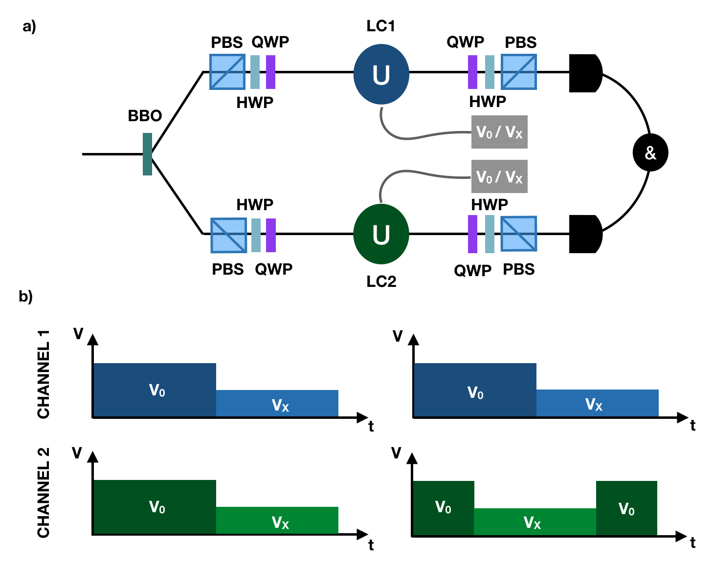
Figure 1: The experiment. a. The setup adopts a nonlinear crystal to generate two-photon states. These are then prepared in the quorum of polarisation states for the capacity witness by means of a polarising beam splitter (PBS), a quarter-wave plate (QWP), and a half-wave plate (HWP). The channel (10) is implemented by a pair of liquid crystal (LC) elements subject to time-varying voltage levels $V_{0}$ and $V_{X}$. Polarisation measurements are carried out by a sequence of QWP-HWP-PBS and single-photon detection. Coincidence measurements are then performed. b. Voltage sequences applied on the two channels for $p=1/2$, in the perfectly correlated $\mu=1$ (left) and uncorrelated $\mu=0$ (right) cases.

The channels’ effect on the photon statistics is simulated using mixtures of operations on the polarisation of single photons. This is for our purposes equivalent to test the witnessing method after a direct implementation of the channel. Photon pairs are produced by parametric down conversion source (CW-pumped at $\lambda_{p}=405$nm, degenerate type-I emission at $\lambda=2\lambda_{p}=810$nm with 7.5nm-bandwidth filters, see Fig. 1a). The active elements are liquid crystal plates, whose birefringence can be varied by applying a voltage. We thus set two different levels for the voltage, namely $V_{0}$, corresponding to the identity, and $V_{X}$, corresponding to the Pauli-X, for different times $t_{0}$ and $t_{X}$, respectively thus defining $p$.

The key to introducing correlations between the two channels is the control of the relative timings of the LCs. Consider, for instance, the case for $p=1/2$: during the total counting time $T_{c}=8$s, on each channel the LCs remain, overall, at $V_{X}$ for $t_{X}=4$s and at $V_{0}$ for $t_{0}=4$s. In the first arm, we simply switch between the two voltage levels halfway during the measurement (Fig. 1b). The two channels will be maximally correlated, $\mu=1$, if we change settings of the LC in the second arm at exactly the same time (Fig. 1b); on the opposite extreme, the channels act independently, $\mu=0$ if the four possible settings $(V_{X},V_{X})$, $(V_{X},V_{0})$, $(V_{0},V_{X})$, and $(V_{0},V_{0})$ all occur for same duration (Fig. 1b). We can access intermediate values of $\mu$ by anticipating the switching time from $V_{0}$ to $V_{X}$ in channel two, ensuring it is switched back again to maintain an equal amount of time for both settings; this also guarantees that $A_{0,X}=A_{X,0}$. The same reasoning can be applied to other values of $p$ and $\mu$, following the prescriptions detailed in Table 1 in the Appendix. Our implementation of the channels is a simple one, and has the advantage of providing good control of the level of correlations. However, we can rely on such realization for our goal of testing the channel capacity witness.

In order to avoid recurring to four-qubits entangled states, the capacity witness has been measured by using the separable-input strategy described in the previous section. In our scheme, we encode the eigenvalues of $\sigma_{Z}$ as the horizontal $|H\rangle$ and vertical $|V\rangle$ polarisations; the eigenvalues of $\sigma_{X}$ as $|D\rangle=(|H\rangle+|V\rangle)/\sqrt{2}$, and $|A\rangle=(|H\rangle+|V\rangle)/\sqrt{2}$; the eigenvalues of $\sigma_{Y}$ as $|L\rangle=(|H\rangle+i|V\rangle)/\sqrt{2}$, and $|R\rangle=(|H\rangle-i|V\rangle)/\sqrt{2}$. All these states can be prepared and measured by a suitable combination of half- and quarter-wave plates [47]. All relevant probabilities are then evaluated based on coincidence count rates; no correction for accidental events and dark counts has been implemented.

When estimating the probabilities in (3), experimental imperfections may lead to small negative values. These are well known artifacts that may occur also in quantum tomography [47]. When these are used in the expression of the entropy, they lead to imaginary values; we found that just considering the real part provides a sufficient regularisation.

We use the single-qubit and two-qubit witness for the combined capacity of the two channels $Q_{\rm tot}$, as well as the capacities of the individual channels $Q_{1}$ and $Q_{2}$. As these bounds are known to be tight, we can adopt $Q_{\rm lim}{=}Q_{1}+Q_{2}$ as the capacity for the independent use of the channels, namely without exploiting the presence of correlations. Therefore, as far as the channel is modelled by Eq. (10), we can assess whether the channels present correlations based on the experimental data. Without any assumption on the form of the channel, the experimental data can only show that the joint use of the channels (whatever they are) provides better bounds to the quantum capacity.

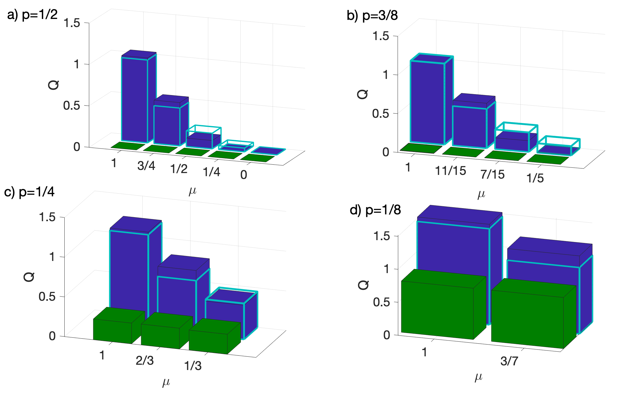
Figure 2: Experimental bounds on the quantum capacity. In all panels, the blue columns represent the experimental values of $Q_{\rm tot}$, to be compared to the green columns indicating the limit $Q_{\rm lim}$ for an independent use of the channels, when ignoring correlations. The cyan edges are the theoretical predictions for the ideal channel (10) given by Eq. (13). Errors are of the order of 0.005, and hence are not visible on this scale.

Our experimental results are depicted in Fig. 2 for the different values of $p$ and $\mu$ considered in our experiment. Whenever the experimental imperfections force a negative lower bound to the capacity, this is replaced with zero. Some discrepancies with respect to the theoretical expectations can be appreciated, mostly due to the fact that the LCs do not implement the operations $\sigma_{0}$ and $\sigma_{X}$ exactly. Appendix 1 reports more experimental details. A direct comparison between theoretical and experimental bounds for $Q_{tot}$ shows that one can not be used as a limit for the other.

IV Discussion

As we can see from the results reported in Fig. 2, the green columns refer to the witness for the total quantum capacity of the local channels, that corresponds to the theoretical values reported in Eq. (13) for $\mu=0$. It is clear from the theoretical expression that for fixed value of $p$ the capacity of the correlated channel is lower bounded by the value of the total capacity of the local channels, and in particular it is an increasing function of $\mu$ at fixed $p$. If the channel that we are observing is guaranteed to be of the form (10), the detection of a capacity larger than the corresponding theoretical value for $\mu=0$ signals the presence of correlations in the channel. This behaviour can be qualitatively identified also in the results reported in Fig. 2, where it is apparent that the blue columns get closer to the green ones for decreasing values of $\mu$. We want to stress, however, that the detection method that we implemented works for any form of channel. In realistic experimental scenarios, a noisy channel will present deviations from its expected model, and in the extreme case the noise could even be completely unknown. Predictions based on a model can give useful indications but would fail at giving a reliable knowledge. On the contrary, the presented method certifies a lower bound to the quantum channel capacity by means of the only experimental data. The major advantage of our method is that it does not need a complete experimental reconstruction of the channel. In fact, this would require full process tomography and would then be much more demanding in terms of measurements required.

Appendix

$p$	$\mu$	$A_{0,0}$	$A_{0,X}$	$A_{X,0}$	$A_{X,X}$	Voltage
1/2	0	1/4	1/4	1/4	1/4
	1/4	5/16	3/16	3/16	5/16
	1/2	3/8	1/8	1/8	3/8
	3/4	7/16	1/16	1/16	7/16
	1	1/2	0	0	1/2
3/8	1/5	3/16	3/16	3/16	7/16
	7/15	1/4	1/8	1/8	1/2
	11/15	5/16	1/16	1/16	9/16
	1	3/8	0	0	5/8
1/4	1/3	1/8	1/8	1/8	5/8
	2/3	3/16	1/16	1/16	11/16
	1	1/4	0	0	3/4
1/8	3/7	1/16	1/16	1/16	13/16
	1	1/8	0	0	7/8

Table 1: Parameters of the channel. The coefficients in (10) are reported for different choices of $p$ and $\mu$, along with a pictorial representation of the sequences of the voltages to channel 1 (blue) and channel 2 (green).

Here we report the measured values of the quantities in (5), pertaining to the operators $X_{i,j}=\sigma_{i}\otimes\sigma_{j}$,with $i,j=X,Y,Z$. Theoretical predictions for the ideal channel in Eq. (10) are:

$$\left(\begin{matrix}1&&-1+2p&&1-2p\\ -1+2p&&1-4p(1-p)(1-\mu)&&-1+4p(1-p)(1-\mu)\\ 1-2p&&-1+4p(1-p)(1-\mu)&&1-4p(1-p)(1-\mu)\end{matrix}\right)$$ (14)

where the $(i,j)$-element in the matrix refers to $\sigma_{i}\otimes\sigma_{j}$, with the index taken in the same order as above.

The recorded values are as follows (errors in brackets):

$p=1/2,\,\mu=0$

$$\left(\begin{matrix}0.9687(5)&&0.020(2)&&0.008(2)\\ 0.002(2)&&0.000(2)&&0.003(2)\\ 0.006(2)&&-0.002(2)&&0.002(2)\\ \end{matrix}\right)$$

$p=1/2,\,\mu=1/4$

$$\left(\begin{matrix}0.9685(5)&&0.012(2)&&0.009(2)\\ 0.007(2)&&0.243(2)&&-0.243(2)\\ 0.006(2)&&-0.240(2)&&0.246(2)\\ \end{matrix}\right)$$

$p=1/2,\,\mu=1/2$

$$\left(\begin{matrix}0.9683(4)&&0.009(2)&&0.013(2)\\ 0.007(2)&&0.483(2)&&-0.487(2)\\ 0.011(2)&&-0.483(2)&&0.487(2)\\ \end{matrix}\right)$$

$p=1/2,\,\mu=3/4$

$$\left(\begin{matrix}0.9680(5)&&0.011(2)&&0.015(2)\\ 0.009(2)&&0.721(2)&&-0.733(2)\\ 0.007(2)&&-0.726(2)&&0.732(2)\\ \end{matrix}\right)$$

$p=1/2,\,\mu=1$

$$\left(\begin{matrix}0.9686(4)&&0.014(2)&&0.013(2)\\ 0.002(2)&&0.9640(4)&&-0.9791(4)\\ 0.009(2)&&-0.9653(4)&&0.9720(5)\\ \end{matrix}\right)$$

$p=3/8,\,\mu=1/5$

$$\left(\begin{matrix}0.9688(6)&&-0.224(2)&&0.253(2)\\ -0.236(2)&&0.237(2)&&-0.245(2)\\ 0.248(2)&&-0.239(2)&&0.244(2)\\ \end{matrix}\right)$$

$p=3/8,\,\mu=7/15$

$$\left(\begin{matrix}0.9695(5)&&-0.225(2)&&0.253(2)\\ -0.237(2)&&0.477(2)&&-0.490(2)\\ 0.249(2)&&-0.479(2)&&0.499(2)\\ \end{matrix}\right)$$

$p=3/8,\,\mu=11/15$

$$\left(\begin{matrix}0.9695(5)&&-0.225(2)&&0.247(2)\\ -0.237(2)&&0.718(2)&&-0.734(2)\\ 0.247(2)&&-0.720(2)&&0.731(2)\\ \end{matrix}\right)$$

$p=3/8,\,\mu=1$

$$\left(\begin{matrix}0.9686(5)&&-0.230(2)&&0.254(2)\\ -0.238(2)&&0.9600(6)&&-0.9784(4)\\ 0.247(2)&&-0.9614(6)&&0.9731(6)\\ \end{matrix}\right)$$

$p=1/4,\,\mu=1/3$

$$\left(\begin{matrix}0.9683(5)&&-0.468(2)&&0.494(2)\\ -0.484(2)&&0.473(2)&&-0.486(2)\\ 0.489(2)&&-0.476(2)&&0.485(2)\\ \end{matrix}\right)$$

$p=1/4,\,\mu=2/3$

$$\left(\begin{matrix}0.9681(6)&&-0.469(2)&&0.496(2)\\ -0.487(2)&&0.711(2)&&-0.732(2)\\ 0.489(2)&&-0.713(2)&&0.734(2)\\ \end{matrix}\right)$$

$p=1/4,\,\mu=1$

$$\left(\begin{matrix}0.9686(5)&&-0.468(2)&&0.495(2)\\ -0.483(2)&&0.9528(5)&&-0.9764(4)\\ 0.490(2)&&-0.9574(6)&&0.9744(6)\\ \end{matrix}\right)$$

$p=1/8,\,\mu=3/7$

$$\left(\begin{matrix}0.9693(5)&&-0.704(2)&&0.734(2)\\ -0.722(2)&&0.708(2)&&-0.732(2)\\ 0.729(2)&&-0.710(2)&&0.736(2)\\ \end{matrix}\right)$$

$p=1/8,\,\mu=1$

$$\left(\begin{matrix}0.9686(5)&&-0.707(2)&&0.738(2)\\ -0.719(2)&&0.9478(5)&&-0.9755(4)\\ 0.729(2)&&-0.9529(6)&&0.9756(4)\\ \end{matrix}\right)$$

References

- [1] C. Macchiavello and G. M. Palma, Phys. Rev. A 65, 050301(R) (2002).
- [2] L. Memarzadeh, C. Macchiavello, and S. Mancini, New J. Phys. 13, 103031 (2011).
- [3] C. Macchiavello, G. M. Palma, and S. Virmani, Phys. Rev. A 69, 010303(R) (2004).
- [4] D. Daems, Phys. Rev. A 76, 012310 (2007).
- [5] Z. Shadman, H. Kampermann, D. Bruss, and C. Macchiavello, Phys. Rev. A 84, 042309 (2011).
- [6] H. Hamada, J. Math. Phys. 43 4382 (2002),
- [7] A. D’Arrigo, G. Benenti, and G. Falci, New J. Phys. 9, 310 (2007).
- [8] M. B. Plenio and S. Virmani, Phys. Rev. Lett. 99, 120504 (2007).
- [9] G. Barreto Lemos and G. Benenti, Phys. Rev. A 81, 062331 (2010).
- [10] N. Arshed, A. H. Toor, and D. A. Lidar, Phys. Rev. A 81, 062353 (2010).
- [11] A. D’Arrigo, G. Benenti, G. Falci, and C. Macchiavello, Phys. Rev. A 88, 042337 (2013); A. D’Arrigo, G. Benenti, G. Falci, and C. Macchiavello, Phys. Rev. A 92, 062342 (2015).
- [12] N.J. Cerf, J. Clavareau, C. Macchiavello, and J. Roland, Phys. Rev. A 72, 042330 (2005).
- [13] O. V. Pilyavets, V. G. Zborovskii, and S. Mancini, Phys. Rev. A 77, 052324 (2008).
- [14] C. Lupo, V. Giovannetti, and S. Mancini, Phys. Rev. Lett. 104, 030501 (2010).
- [15] A. Bayat, D. Burgarth, S. Mancini, and S. Bose, Phys. Rev. A 77, 050306(R) (2008).
- [16] V. Giovannetti and G. M. Palma, Phys. Rev. Lett. 108, 040401 (2012).
- [17] G. Benenti, A. D’Arrigo, and G. Falci, Phys. Rev. Lett. 103, 020502 (2009); A. D’Arrigo, G. Benenti, and G. Falci, Eur. Phys. J. D 66, 147 (2012).
- [18] F. Caruso, V. Giovannetti, C. Lupo, and S. Mancini, Rev. Mod. Phys. 86, 1203 (2014).
- [19] I.L. Chuang, and M.A. Nielsen, J. Mod. Opt. 44, 2455 (1997).
- [20] M. Lobino et al., Science 322, 563 (2008).
- [21] B. Ndagano, et al., Nature Physics 13, 397 (2017).
- [22] F. Bouchard et al., Quantum 3, 138 (2019).
- [23] C. Macchiavello and M. Rossi, Phys. Rev. A 88, 042335 (2013).
- [24] D. Chruscinski, C. Macchiavello and S. Maniscalco, Phys. Rev. Lett. 118, 080404 (2017).
- [25] C. Macchiavello and M. F. Sacchi, Phys. Rev. Lett. 116, 140501 (2016).
- [26] C. Macchiavello and M. F. Sacchi, Phys. Rev. Lett. 123, 090503 (2019).
- [27] A. Cuevas, M. Proietti, M. A. Ciampini, S. Duranti, P. Mataloni, M. F. Sacchi, and C. Macchiavello, Phys. Rev. Lett. 119, 100502 (2017).
- [28] C. Macchiavello and M. F. Sacchi, Phys. Rev. A 94, 052333 (2016).
- [29] S. Lloyd, Phys. Rev. A 55, 1613 (1997).
- [30] H. Barnum, M. A. Nielsen, and B. Schumacher, Phys. Rev. A 57, 4153 (1998).
- [31] I. Devetak, IEEE Trans. Inf. Theory 51, 44 (2003).
- [32] B. W. Schumacher and M. A. Nielsen, Phys. Rev. A 54, 2629 (1996).
- [33] B. W. Schumacher, Phys. Rev. A 54, 2614 (1996).
- [34] M. A. Nielsen and I. L. Chuang, Quantum Information and Communication (Cambridge, Cambridge University Press, 2000).
- [35] G. M. D’Ariano, P. Lo Presti, and M. F. Sacchi, Phys. Lett. A 272, 32 (2000).
- [36] M. Barbieri, F. De Martini, G. Di Nepi, P. Mataloni, G. M. D’Ariano, and C. Macchiavello, Phys. Rev. Lett. 91, 227901 (2003).
- [37] M. Bourennane, M. Eibl, C. Kurtsiefer, S. Gaertner, H. Weinfurter, O. Gühne, P. Hyllus, D. Bruss, M. Lewenstein, and A. Sanpera, Phys. Rev. Lett. 92, 087902 (2004).
- [38] Z.-D. Li, Q. Zhao, R. Zhang, L.-Z. Liu, X.-F. Yin, X. Zhang, Y.-Y. Fei, K. Chen, N.-L. Liu, F. Xu, Y.-A. Chen, L. Li, and J.-W. Pan Phys. Rev. Lett. 124, 160503 (2020).
- [39] Y.-C. Liang, D. Rosset, J.-D. Bancal, G. Pütz, T. J. Barnea, and N. Gisin Phys. Rev. Lett. 114, 190401 (2015).
- [40] Y. Zhou, Q. Zhao, X. Yuan, and X. Ma npj Quantum Info 5, 83 (2019)
- [41] Y.-Q. Nie, H. Zhou, J.-Y. Guan, Q. Zhang, X. Ma, J. Zhang, and J.-W. Pan Phys. Rev. Lett. 123, 090502 (2019).
- [42] M. Ringbauer, T. R. Bromley, M. Cianciaruso, L. Lami, W.Y.S. Lau, G. Adesso, A. G. White, A. Fedrizzi, and M. Piani Phys. Rev. X 8, 04100 (2018).
- [43] C.-M. Li, N. Lambert, Y.-N. Chen, G.-Y. Chen, and F. Nori, Sci. Rep. 2, 885 (2012).
- [44] A. Mari, K. Kieling, B. M. Nielsen, E. S. Polzik and J. Eisert, Phys. Rev. Lett. 106, 010403 (2011).
- [45] K. Laiho, K. N. Cassemiro, D. Gross, and C. Silberhorn Phys. Rev. Lett. 105, 253603 (2010).
- [46] Kalev, A., Kosut, R., and Deutsch, I., npj Quantum Inf. 1, 15018 (2015)
- [47] D.F.V. James, P.G. Kwiat, W.J. Munro, and A.G. White Phys. Rev. A 64, 052312.
- [48] Kim, Y., Teo, Y. S., Ahn, D., Im, D.-G., Cho, Y.-W., Leuchs, G., Sánchez-Soto, L. L., Jeong, H., and Kim, Y.-H., Phys. Rev. Lett. 124, 210401 (2020)
- [49] Teo, Y. S., Englert, B.-G., Řeháček, J., and Hradil, Z., Phys. Rev. A, 84, 062125, (2011)
- [50] Kim, Y., Kim, Y., Lee, S., Han, S.-W., Moon, S., Kim, Y.-H., and Cho, Y.-W., Nat. Commun. 9, 192 (2018)
- [51] M. Mohseni, A. T. Rezakhani, and D. A. Lidar, Phys. Rev. A 77, 03232 (2008).