On lengths of burn-off chip-firing games

Abstract

We continue our studies of burn-off chip-firing games from [Discrete Math. Theor. Comput. Sci. 15 (2013), no. 1, 121–132; MR3040546] and [Australas. J. Combin. 68 (2017), no. 3, 330–345; MR3656659]. The latter article introduced randomness by choosing successive seeds uniformly from the vertex set of a graph $G$. The length of a game is the number of vertices that fire (by sending a chip to each neighbor and annihilating one chip) as an excited chip configuration passes to a relaxed state. This article determines the probability distribution of the game length in a long sequence of burn-off games. Our main results give exact counts for the number of pairs $(C,v)$, with $C$ a relaxed legal configuration and $v$ a seed, corresponding to each possible length. In support, we give our own proof of the well-known equicardinality of the set $\mathcal{R}$ of relaxed legal configurations on $G$ and the set of spanning trees in the cone $G^{*}$ of $G$. We present an algorithmic, bijective proof of this correspondence.

Keywords: chip-firing, burn-off game, relaxed legal configuration, spanning tree, Markov chain, game-length probability, sandpile group

In recognition of Gary MacGillivray’s milestone birthday in 2020 No jokes in the paper, but not so in the talk!

1 Introduction

This article continues our study in [19] and [24] of burn-off chip-firing games, in which each iteration simulates the loss of energy from a complex system. These games are played on graphs and consist of a sequence of ‘seed-then-relax’ steps, wherein a chosen vertex is excited (by adding a ‘chip’ to it) after which the system (i.e. a graph containing chips on its vertices) is allowed to ‘relax’. During relaxation, certain vertices ‘fire’ (by sending chips to their neighbors and annihilating a chip); the ‘length’ of a game is the number of such vertices. We shall see that the firing order and number of firings at any given moment has no effect on the eventual relaxation; so, e.g., the notion of length is well defined (see Lemmas 2.1 and 2.2). In [24], we introduced randomness to these games by choosing each successive seed uniformly at random from among all possible vertices. The present work aims primarily at shedding light on the probability distribution of the game length in a long sequence of burn-off games. Our main results in this direction—Proposition 4.1 and Theorem 4.2—give exact counts for the number of pairs $(C,v)$, with $C$ a ‘relaxed legal chip configuration’ and $v$ a seed vertex, corresponding to each possible game length.

En route to these results, we (re)discovered that, for a graph $G$, our set $\mathcal{R}$ of relaxed legal configurations on $G$ is equicardinal to the set $\mathcal{S}$ of spanning trees in the ‘cone’ $G^{*}$ of $G$. We present an algorithmic, bijective proof of this fact in Section 3 (Theorem 3.1). The connection between chip firing and spanning tree enumeration has been addressed by numerous authors (e.g., [4], [5], [6], [7], [17], [19]), but we present our take for several reasons. First, our main results in Section 4 rest on ideas in our proof in Section 3. Second, that

$$|\mathcal{R}|=|\mathcal{S}|$$ (1)

is a key connecting $\mathcal{R}$ with the ‘sandpile group’ $K(G^{*})$; thus we recover an appealing description of the elements of this group. Finally, we hope that our constructive proof stands up, of interest in its own right.

We attempt neither a literature review nor a discussion of background or motivation for chip firing. Perhaps the most immediate resource for related material is David Perkinson’s beautiful Sandpiles website [26], which, besides literature links, provides access to simulation software including Sage tools. We also point the reader to our other papers [19], [24], [25], to the surveys [17], [22], to the books [12], [20], and to the concise but thorough AMS column [21].

The rest of this article is organized as follows. First (in Section 1.1), we introduce the basic chip-firing notions, including the undefined terms already encountered. In Section 1.2, we take a brief detour to explain the connection between $\mathcal{R}$ and $K(G^{*})$ implied by (1). Section 2 details the earlier lemmas and tools supporting our main results. In Section 3, we present our proof of (1). Our main results counting pairs $(C,v)\in\mathcal{R}\times V$ with specified game lengths appear in Section 4. In Section 5, we close with an example illustrating the use of Theorem 3.1, Proposition 4.1, and Theorem 4.2 in determining the probability distribution for game length.

Notation and terminology

In this paper, all graphs are finite, simple, and undirected. We usually think of playing burn-off games on connected graphs, but most of our results don’t require connectivity; cf. the first paragraph in the proof of Theorem 3.1. We use ‘general graph’ when we wish to emphasize that a graph may be disconnected. The order of a graph $G=(V,E)$ is denoted by $n$ ($:=|V|$). If $G$ has a subgraph $X$ and $v\in V(G)$, then $\Gamma_{X}(v)$ denotes the set of neighbors of $v$ that lie in $V(X)$. If $G$ is connected and $u,v\in V$, then the least length of a $uv$-path in $G$ is the distance $d_{G}(u,v)$ from $u$ to $v$. Finally, we write $\tau=\tau(G)$ for the number of spanning trees of $G$.

We mainly follow usual graph theory conventions as found, e.g., in [9] and refer the reader there for any omitted items of this sort. A graph theory reference that addresses chip firing specifically is [16]. For probability background, see the classic [15].

1.1 Burn-off chip firing

Beginning with a (chip) configuration on a graph $G=(V,E)$—i.e., a function $C\colon V\to\mathbb{N}$—a burn-off (chip-firing) game plays as follows. For a vertex $v$, if $C(v)$ exceeds $\deg_{G}(v)$, then $v$ can fire, meaning it sends one chip to each neighbor and one chip into ‘thin air’. Formally, when $v$ fires, $C$ is modified to a configuration $C^{\prime}$ such that

$$C^{\prime}(u)=\left\{\begin{array}[]{ll}C(v)-\deg_{G}(v)-1&\text{if }u=v,\\ C(u)+1&\text{if }uv\in E(G),\\ C(u)&\text{if }v\neq u\not\sim v.\end{array}\right.$$ (2)

As we noted in [19], the game just defined is equivalent to the ‘dollar game’ of Biggs [7] in the case when his ‘government’ vertex is adjacent to every other vertex in the underlying graph; it is also equivalent to the sandpile model on $G^{*}$ (see, e.g., [17]).

For a configuration $C$, a vertex $v$ is critical if $C(v)=\deg_{G}{(v)}$ and supercritical if $C(v)>\deg_{G}{(v)}$. A relaxed configuration is one for which no vertex can fire. To start a burn-off game, we add a chip to a selected vertex $v$ (called a seed) in a relaxed configuration $C$. This is called seeding $C$ at $v$ and is sometimes denoted algebraically: by writing $\mathbf{1}_{v}$ for the configuration with a total of one chip, on $v$ only, and passing from $C$ to $C+\mathbf{1}_{v}$. Just prior to seeding, if $v$ happened to be critical, then from $C+\mathbf{1}_{v}$, we fire $v$, which may trigger a neighbor $u$ of $v$ to become supercritical. If so, we fire $u$, which may trigger another vertex to become supercritical. The game follows this cascade until reaching a relaxed configuration, called a relaxation of $C+\mathbf{1}_{v}$. The game length equals the number of vertex firings, possibly zero, in passing from the initial relaxed configuration to the final one.

In a long game sequence, certain sparse configurations will cease to appear after enough seedings. Let us suppose, for example, that a game sequence is initialized with the all-zeros configuration. Except on a trivial graph, this configuration will never recur, and a configuration $\mathbf{1}_{v}$ on a triangle ($K_{3}$) also will never be seen after its first occurence. Loosely speaking, by ‘legal’ configurations, we mean those typically encountered in a long game sequence. To define these formally, we begin by calling a configuration supercritical if every vertex is supercritical. We follow our earlier papers [19], [24], and focus on the configurations that can result from relaxing supercritical ones. First consider what happens when a burn-off game is played in reverse. Considering (2), we see that to start in a configuration $C^{\prime}$ and reverse-fire a vertex $v$ (each of whose neighbors $u$ necessarily satisfies $C^{\prime}(u)\geq 1$) means to modify $C^{\prime}$ to a configuration $C$ such that

$$C(u)=\left\{\begin{array}[]{ll}C^{\prime}(v)+\deg_{G}(v)+1&\text{if }u=v,\\ C^{\prime}(u)-1&\text{if }uv\in E(G),\\ C^{\prime}(u)&\text{if }v\neq u\not\sim v.\end{array}\right.$$

Now a configuration $C$ is legal if there exists a reverse-firing sequence starting with $C$ and ending with a supercritical configuration. Throughout this paper, we use $\mathcal{R}=\mathcal{R}(G)$ to denote the set of relaxed legal configurations on $G$.

A relaxed configuration $C$ is recurrent if, given any (unrestricted) configuration $C^{\prime}$, it is possible to pass from $C^{\prime}$ to $C$ via a sequence of seeding vertices and firing supercritical ones.

1.2 The sandpile group

As mentioned following (1), the set $\mathcal{R}$ is linked to $G^{*}$’s sandpile group, which we proceed to define (see Section 3 for a definition of $G^{*}$ itself). Start by viewing configurations $C\colon V\to\mathbb{N}$ as elements of the group $\mathbb{Z}^{V}$. Looking at (2), notice that firing a vertex $v\in V$ corresponds to adding to $C$ the vector $\Delta_{v}\in\mathbb{Z}^{V}$ with entries

$$\Delta_{v,u}:=\left\{\begin{array}[]{cl}-\deg_{G^{*}}(v)&\text{if }u=v,\\ 1&\text{if }uv\in E(G),\\ 0&\text{if }v\neq u\not\sim v,\end{array}\right.$$

in which $u$ runs through $V$. The matrix $\Delta:=(\Delta_{v,u})=(\Delta_{u,v})$ is the reduced Laplacian of $G^{*}$ (“reduced” as it omits the row/column corresponding to the universal vertex introduced in passing from $G$ to $G^{*}$), and thus we see that chip firing provides a natural setting for the appearance of $\Delta$ (see, e.g., [9] for background on the graph Laplacian). The idea that configurations appearing in a sequence of vertex firings enjoy an intimate connection motivates calling two configurations $C$, $D$ firing equivalent exactly when $C-D$ lies in the $\mathbb{Z}$-linear span $\Delta\mathbb{Z}^{V}$ of the vectors $\Delta_{v}$, i.e., when $C$ and $D$ lie in the same coset of the quotient group $\mathbb{Z}^{V}/\Delta\mathbb{Z}^{V}$. This is the sandpile group of $G^{*}$ and is denoted by $K(G^{*})$. Our discussion here follows [21], which gives a chockablock introduction to the subject.

Before presenting our own results, we record an observation on the role of (1) in connecting $\mathcal{R}$ with $K(G^{*})$.

Proposition 1.1.

The elements of $\mathcal{R}$ can serve as a set of representatives for $K(G^{*})$.

Proof.

First note that both of $\mathcal{R}$, $K(G^{*})$ contain $\tau(G^{*})$ elements. For $\mathcal{R}$ , this is (1) (our Theorem 3.1) and for $K(G^{*})$, this is also well known (see, e.g., [21]). Furthermore, members of $\mathcal{R}$ are all recurrent configurations, a fact we proved in [24, Proposition 3.1] (though it was known much earlier in the sandpile literature; cf. [13]). Now each equivalence class of $\mathbb{Z}^{V}$ (under the firing equivalence) contains exactly one recurrent configuration (see [21] again, or, e.g., [17]). So we have $\tau(G^{*})$ recurrent configurations (in $\mathcal{R}$) and the same number of recurrent configurations appearing among the elements of $K(G^{*})$ (i.e., among the the equivalence classes of $\mathbb{Z}^{V}$), the latter being exhaustive. Therefore, $\mathcal{R}$ must be the set of all recurrent configurations. ∎

Proposition 1.1 is not new. Indeed, it recasts the modern definition of $K(G^{*})$ above in terms of the original definition due to Dhar [13]. Nevertheless, it’s striking to observe the central role that enumeration plays in its proof.

2 Supporting results

In Section 1.1, we glossed over whether the length of a burn-off game is well defined. The following early chip-firing result settles this question and shows that the relaxation of a configuration is uniquely determined.

Lemma 2.1 ([13],[14]).

In a burn-off game on a general graph, the vertices can be fired in any order without affecting the length or final configuration of the game.

Lemma 2.1 has appeared in several other places, including [8], [17], and [23], the second of these containing a particularly succinct proof.

Because our graphs are finite and a chip is burned during every vertex-firing, burn-off games of infinite length are impossible. Within the general chip-firing literature, finding non-trivial bounds for the game length has been tackled more than once; see, e.g., [28] and [29]. For our purposes, we shall need the following elementary result.

Lemma 2.2.

During a burn-off game that starts with a relaxed legal configuration, no vertex fires more than once.

In the sandpile literature, Lemma 2.2 originated in [13] as elucidated in [11]. Before we became aware of its earlier existence, the second author of the present work included it in his dissertation [23] and we included a proof in [24].

Our last three tools concern legal configurations. They appeared in [23], followed by published proofs in [19]. Likewise with Lemma 2.2, their versions in the sandpile literature predate these citations; for example, the first tool—Lemma 2.3—follows from the correctness of Algorithm 2.5 so dates to [13]. It characterizes the relaxed legal configurations on general graphs $G$. In its statement, $N_{G}$ denotes the ‘earlier neighbor’ set; i.e., given an ordering $(w_{1},\ldots,w_{n})$ of $V(G)$, we define $N_{G}(w_{i}):=\{w_{j}\colon w_{i}w_{j}\in E(G)\text{ and }j<i\}$.

Lemma 2.3.

A relaxed configuration $C\colon V\to\mathbb{N}$ is legal if and only if it is possible to relabel $V$ as $w_{1},\ldots,w_{n}$ so that

$$C(w_{i})\geq|N_{G}(w_{i})|\text{ for }1\leq i\leq n.$$ (3)

The following basic result establishes that containing a legal configuration is an inherited property for graphs; see [19] for one published proof.

Lemma 2.4.

For a configuration $C\colon V(G)\to\mathbb{N}$ and a subgraph $H$ of $G$, if $C$ is legal on $G$, then $C|_{V(H)}$ is legal on $H$.

We close this section by recalling an algorithm for determining the legality of a given configuration. The version stated here is from [19]—a published account from [23]—but it’s essentially Dhar’s ‘Burning Algorithm’ from [13]; see also [11]. The proofs of Theorems 3.1 and 4.2 use this algorithm repeatedly.

Algorithm 2.5.

Input:	a graph $G=(V,E)$ and a chip configuration $C\colon V\to\mathbb{N}$ on $G$
Output:	an answer to the question ‘Is $C$ legal?’
(1)	Let $\widehat{G}=G$.
(2)	If $C(v)<\deg_{\widehat{G}}(v)$ for all $v\in V(\widehat{G})$, then stop; output ‘No’.
(3)	Choose any $v\in V(\widehat{G})$ with $C(v)\geq\deg_{\widehat{G}}(v)$.
(4)	Delete $v$ and all incident edges from $\widehat{G}$ to create a graph $G^{-}$.
(5)	If $V(G^{-})=\varnothing$, then stop; output ‘Yes’.
(6)	Let $\widehat{G}=G^{-}$ and go to step 2.

3 Enumerating relaxed legal configurations

Here we present our proof of (1). For a graph $G$, recall that the cone $G^{*}$ is obtained from $G$ by adding a new vertex $x$ adjacent to every vertex of $G$. This derived graph is sometimes called the ‘suspension’ of $G$ over $x$, but we shall not use this term. The reader should keep in mind the special role that the symbol ‘$x$’ plays in this section and the next.

Theorem 3.1.

The number of relaxed legal configurations on $G$ is the number of spanning trees of $G^{*}$.

Proof.

We may assume that $G$ is connected, for if $H_{1},\ldots,H_{k}$ are the components of $G$, then—once we have $|\mathcal{R}(H_{i})|=\tau(H_{i}^{*})$ for $1\leq i\leq k$ (i.e., once we have the theorem for connected graphs)—we obtain

$$|\mathcal{R}(G)|=\prod_{i=1}^{k}|\mathcal{R}(H_{i})|=\prod_{i=1}^{k}\tau(H_{i}^{*})=\tau(G^{*}),$$

which is the theorem for general graphs.

Given a connected graph $G$, we establish algorithmically injections back and forth between $\mathcal{R}$ and the set $\mathcal{S}$ of spanning trees of $G^{*}$. Define $A\colon\mathcal{R}\to\mathcal{S}$ via Algorithm 3.2 below and $B\colon\mathcal{S}\to\mathcal{R}$ via Algorithm 3.3 below.

Algorithm 3.2.

Input:	a connected graph $G=(V,E)$ with $V=\{v_{1},v_{2},\ldots,v_{n}\}$ and a configuration $C\in\mathcal{R}$
Output:	a spanning tree $A(C)=T^{*}$ of $G^{*}$
(0)	Let $T^{*}$ be the subgraph of $G^{*}$ with $V(T^{*})=\{x\}$, $E(T^{*})=\varnothing$.
(1)	Let $i=1$.
(2)	Let $M_{1}$ be the sequence (in increasing subscript order) of vertices $v_{k}$ such that $C(v_{k})=\deg_{G}(v_{k})$; let $\overline{M}_{1}=\{x\colon x\text{ is an entry of }M_{1}\}$.
(3)	For each $v_{k}\in\overline{M}_{1}$, add $v_{k}$ to $V(T^{*})$ and $\{x,v_{k}\}$ to $E(T^{*})$; if $V(T^{*})=V$, then stop.
(4)	$i\mathrel{\reflectbox{$\mapsto$}}i+1$.
(5)	Let $M_{i}$ be the sequence (in increasing subscript order) of the vertices not yet included in $V(T^{*})$ that are neighbors of vertices in $M_{i-1}$; let $\overline{M}_{i}=\{x\colon x\text{ is an entry in }M_{i}\}$.
	For each $u\in\overline{M}_{i}$, execute steps (6) through (9):
(6)	For $r=1,2,\ldots,i-1$, let $N_{r}=(v_{r,1},v_{r,2},\ldots,v_{r,k_{r}})$ be the sequence (in increasing subscript order) of the $k_{r}$ $G$-neighbors of $u$ that appear in $\overline{M}_{r}$; let $\overline{N}_{r}=\{x\colon x\text{ is an entry in }N_{r}\}$.
(7)	Let $s=\left|\bigcup_{r=1}^{i-1}{\overline{N}_{r}}\right|$ and $N=(v_{\ell_{1}},v_{\ell_{2}},\ldots,v_{\ell_{s}})$ be the sequence determined by concatenating the sequences $N_{1},N_{2},\ldots,N_{i-1}$.
(8)	If $C(u)<\deg_{G}(u)-s$, then delete $u$ from $M_{i}$ and $\overline{M}_{i}$.
(9)	Otherwise, $C(u)=\deg_{G}(u)-j$ for some $j$ with $1\leq j\leq s$; add $u$ to $V(T^{*})$ and $\{u,v_{\ell_{j}}\}$ to $E(T^{*})$.
(10)	If $V(T^{*})=V$, then stop; otherwise, go to step (4).

Proof that $A$ is well-defined. Not only must we be sure that Algorithm 3.2 outputs a spanning tree $T^{*}$, but also we must check that it does not halt before doing so. To establish both of these results, we look at each step in turn.

Step (2). By Algorithm 2.5, we know that at least one vertex in a legal configuration contains at least as many chips as its degree. Thus $\overline{M}_{1}$ is not empty.

Step (3). It is clear that $T^{*}$ is thus far a tree; in fact, it is a star.

Step (5). We must establish that $\overline{M}_{i}$ is nonempty so that the “for each $u\in\overline{M}_{i}$” instruction is not quantifying over an empty set. We proceed by induction. In the discussion of Step (2) above, we observed that $\overline{M}_{1}$ is nonempty. By construction, all vertices in $\overline{M}_{1}$ are critical. Because $C$ is a legal configuration, we may apply Algorithm 2.5 to $G$ and delete all of the vertices (in any order) in $\overline{M}_{1}$.

With these statements as our base case, our induction hypothesis is in two parts: for fixed $i>1$, suppose that (a) $\overline{M}_{1},\overline{M}_{2},\ldots,\overline{M}_{i-1}$ are nonempty; and (b) we may apply Algorithm 2.5 to $G$ and delete the vertices in $\overline{M}_{1},\overline{M}_{2},\ldots,\overline{M}_{i-1}$ without halting.

Let $M=\bigcup_{j=1}^{i-1}{\overline{M}_{j}}$. Lemma 2.4 states that the configuration on any subgraph of a graph (on which we have a legal configuration) must itself be legal. So, if our application of Algorithm 2.5 has deleted exactly the vertices of $M$, then at least one of the remaining vertices $u$ of $G-M$ must be critical in $G-M$. Suppose that $u$ is not a neighbor of any vertex in $M$. Because $u$ is critical in $G-M$, and none of its neighbors have been deleted in our application of Algorithm 2.5, we see that $u$ is also critical in $G$. But this places $u$ in $\overline{M}_{1}$, which contradicts the choice of $u$ in $G-M$.

Thus, we know that $u$ is a neighbor of some vertex in $M$. Now if $u$ is not a neighbor of a vertex in $\overline{M}_{i-1}$, it must be adjacent to, say, $s\geq 1$ vertices in $\overline{M}_{1},\overline{M}_{2},\ldots,\overline{M}_{i-2}$. Thus, $u$ has been considered previously by step (8) and has been deleted each time. Therefore, $C(u)<\deg_{G}(u)-s$. This shows (back in our application of Algorithm 2.5) that if we have deleted all of the vertices in $\overline{M}_{1},\overline{M}_{2},\ldots,\overline{M}_{i-1}$, including the $s$ neighbors of $u$, then $u$ will not be critical in $G-M$. This contradicts the fact that $u$ is critical in $G-M$, so $u$ must be a neighbor of a vertex in $\overline{M}_{i-1}$.

Because $u$ is critical in $G-M$, step (8) will not delete $u$ from $\overline{M}_{i}$. Thus, $\overline{M}_{i}$ is nonempty; this fulfills part (a) of the induction hypothesis. We claim that any vertex $w$ placed in $\overline{M}_{i}$ by step (5) will survive past step (8) only if it, too, is critical in $G-M$. For $w$ to survive step (8), we require that $C(w)\geq\deg_{G}(w)-s$, where $s$ is the number of $G$-neighbors of $w$ that appear in $M$. Since $\deg_{G}(w)-s$ simply equals $\deg_{G-M}(w)$, we know that $w$ is critical in $G-M$. Thus, all vertices in $\overline{M}_{i}$ can be deleted as we apply Algorithm 2.5. This fulfills part (b) of the induction hypothesis.

Step (6). Step (5) ensures that these neighbors exist.

Step (8). The argument given above for step (5) ensures that $\overline{M}_{i}$ remains nonempty after all vertices of $\overline{M}_{i}$ have been processed in step (8).

Step (9). It is impossible to create a cycle in this step because step (5) only considers those vertices that are not yet part of $V(T^{*})$.

Step (10). This step ensures that $T^{*}$ will be a spanning tree of $G^{*}$.

Observe that step (9) adds at least one edge to $T^{*}$ since $\overline{M}_{i}$ remains nonempty. Once $n-1$ edges have been added to $T^{*}$, step (10) will halt the algorithm. Since Algorithm 3.2 does not halt until it outputs a spanning tree $T^{*}$, the function $A$ is well-defined. ∎

Proof that $A$ is an injection. Let $C\in\mathcal{R}$ and $C^{\prime}\in\mathcal{R}$ be two distinct relaxed legal configurations on $G$. We prove that $A$ is an injection by showing that the spanning trees $A(C)$ and $A(C^{\prime})$ must be distinct. As Algorithm 3.2 operates on $C$ and $C^{\prime}$, it must encounter a vertex $v$ for which $C(v)\neq C^{\prime}(v)$. Step (8) might remove $v$ from consideration; if this occurs for both inputs $C$ and $C^{\prime}$, then we consider a future pass of the algorithm. Because Algorithm 3.2 includes every vertex in the output before it halts, we know that eventually we will find a vertex $v$ for which $C(v)\neq C^{\prime}(v)$ that is not removed by step (8) concurrently for both inputs $C$ and $C^{\prime}$.

Now if $v$ is removed by step (8) for one input but not the other, then step (9) will connect $v$ to a different neighbor for the two inputs. On the other hand, suppose that $v$ is not removed by step (8) for either input; because $C(v)\neq C^{\prime}(v)$, step (9) will connect $v$ to a different neighbor for the two inputs. In either case, $A(C)$ and $A(C^{\prime})$ must be distinct, and $A$ is an injection. ∎

Algorithm 3.3.

Input:	a spanning tree $T^{*}$ of $G^{*}$ along with an ordering $V=(v_{1},v_{2},\ldots,v_{n})$ of the vertices in $G$
Output:	a relaxed legal configuration $B(T^{*})=C\in\mathcal{R}$
(1)	Let $M_{0}=(x)$.
(2)	Let $m=\max_{v\in V}\{d_{T^{*}}(x,v)\}$. For $j=1,2,\ldots,m$, let $M_{j}$ be the sequence (in breadth-first order, breaking ties lexicographically by subscript) of vertices $v$ for which $d_{T^{*}}(x,v)=j$; let $\overline{M}_{j}=\{x\colon x\text{ is an entry of }M_{j}\}$.
(3)	For each $u\in\overline{M}_{1}$, let $C(u)=\deg_{G}(u)$.
	For $i=2,3,\ldots,m$ and for each $u\in\overline{M}_{i}$, following the ordering in $M_{i}$, execute steps (4) through (7):
	(4) For $r=1,2,\ldots,i-1$, let $N_{r}=(v_{r,1},v_{r,2},\ldots,v_{r,k_{r}})$ be the sequence (in their $M_{r}$-ordering) of the $k_{r}\geq 0$ $G$-neighbors of $u$ that appear in $M_{r}$; let $\overline{N}_{r}=\{x\colon x\text{ is an entry of }N_{r}\}$. (5) Let $s=\left|\bigcup_{r=1}^{i-1}{\overline{N}_{r}}\right|$. (6) Let $N=(v_{h_{1}},v_{h_{2}},\ldots,v_{h_{s}})$ be the sequence determined by concatenating the sequences $N_{1},N_{2},\ldots,N_{i-1}$. (7) For some $t\in\{1,2,\ldots,s\}$, we have $\{v_{h_{t}},u\}\in E(T^{*})$; let $C(u)=\deg_{G}(u)-t$.

Proof that B is well-defined. In step (2), we partition $V$ into the sequences $M_{1},M_{2},\ldots,M_{m}$. Step (3) assigns chips to the vertices in $\overline{M}_{1}$, while step (7) assigns chips to the vertices in $\overline{M}_{2},\ldots,\overline{M}_{m}$. Therefore, Algorithm 3.3 at least produces a function $C\colon V\to\mathbb{N}$.

Now we use Algorithm 2.5 to establish that $C$ is legal. Since $T^{*}$ is a spanning tree of $G^{*}$, we know that $\overline{M}_{1}$ is nonempty (see step (3)); hence, there is at least one vertex $u$ such that $C(u)=\deg_{G}(u)$. Thus Algorithm 2.5, given $C$ as input, can delete the vertices in $\overline{M}_{1}$. This fact is the base case in an induction argument that proves that in Algorithm 2.5, the vertices in $\overline{M}_{1},\overline{M}_{2},\ldots,\overline{M}_{m}$ can be deleted in the order given by this list. Suppose that this is true for $\overline{M}_{1},\overline{M}_{2},\ldots,\overline{M}_{k-1}$, where $2\leq k<m$. For any $u\in\overline{M}_{k}$, step (7) assigns $C(u)=\deg_{G}(u)-t\geq\deg_{G}(u)-s$. Recall that $s$ counts the neighbors in $G$ of $u$ that are in $\cup_{r=1}^{i-1}{\overline{M}_{r}}$; in our induction hypothesis, we have assumed that these neighbors have been deleted from $G$, resulting, say, in a subgraph $G^{\prime}$. If other vertices in $\overline{M}_{k}$ have been deleted before we consider $u$, then $\deg_{G^{\prime}}(u)$ does not increase. Thus, we have $C|_{V(G^{\prime})}(u)\geq\deg_{G^{\prime}}(u)$, so $u$ can be deleted by Algorithm 2.5. ∎

Proof that B is an injection. Suppose that $T^{*}_{1},T^{*}_{2}\in\mathcal{S}$ satisfy

$$C_{1}:=B(T^{*}_{1})=B(T^{*}_{2})=:C_{2}(:=C);$$

we show that then $T^{*}_{1}=T^{*}_{2}$.

Write the breadth-first orderings of $V$ determined during the computation of $B(T^{*}_{1})$ and $B(T^{*}_{2})$ as $(u_{i})_{i=1}^{n}$ and $(w_{i})_{i=1}^{n}$, respectively. To complete the proof, we shall find it useful to establish the following lemma.

Lemma 3.4.

Under the hypothesis that $C_{1}=C_{2}$, if there exists an integer $j\geq 1$ such that $u_{i}=w_{i}$ for all $i\in\{1,\ldots,j\}$, then the subtree $H^{*}_{1}$ of $T^{*}_{1}$ induced on $\{x,u_{1},\ldots,u_{j}\}$ is identical to the subtree $H^{*}_{2}$ of $T^{*}_{2}$ induced on $\{x,w_{1},\ldots,w_{j}\}$.

Proof.

We induct on $j$. First note that $H^{*}_{1}$, $H^{*}_{2}$ are indeed subtrees of $T^{*}_{1},T^{*}_{2}$, respectively, since the sequences $(u_{i}),(w_{i})$ are defined by breadth-first searches on these trees. It is also clear from the definitions of $(u_{i})$, $(w_{i})$ that $u_{1}$, $w_{1}$ are adjacent to $x$ in $H^{*}_{1}$, $H^{*}_{2}$, respectively. In the case where $j=1$, these subtrees both consist of $2$-vertex trees containing the edge $\{x,u_{1}\}=\{x,w_{1}\}$ and are therefore identical.

Now fix $j>1$, assume that the lemma holds for smaller instances of $j$, and suppose that $u_{i}=w_{i}$ for all $i\in\{1,\ldots,j\}$. Let $G^{*}_{0}$ denote the subgraph of $G^{*}$ induced on the common vertex set $U:=\{x,u_{1},\ldots,u_{j}\}$ of $H^{*}_{1}$, $H^{*}_{2}$, and let $G_{0}=G^{*}_{0}-x$. We consider four executions of Algorithm 3.3; in each case, the input vertex ordering is inherited from $G$.

The first pair of executions computes $D_{1}:=B(H^{*}_{1})$ and $D_{2}:=B(H^{*}_{2})$, two configurations on $G_{0}$. Since $(u_{i})_{i=1}^{j}$, $(w_{i})_{i=1}^{j}$ are initial segments of $(u_{i})$, $(w_{i})$, it is evident from Algorithm 3.3 that $D_{1}$, $D_{2}$ are obtained from $C_{1}$, $C_{2}$ by replacing $\deg_{G}$ in steps (3),(7) by $\deg_{G_{0}}$ and restricting the resulting functions to $U$. Since $C_{1}=C_{2}$, we have $D_{1}=D_{2}$. For $k=1,2$ and for each vertex $u\in V(G_{0})$, let $t_{k}(u)$ denote the value of $t$ in step (7) as Algorithm 3.3 determines $D_{k}(u)$; if $D_{k}(u)$ is determined in step (3), we take $t_{k}(u):=0$. Then

$$D_{k}(u)=\deg_{G_{0}}(u)-t_{k}(u)\text{ for }k=1,2\text{ and each }u\in V(G_{0}).$$ (4)

The second pair of executions computes $D^{\prime}_{1}:=B(H^{*}_{1}-u_{j})$ and $D^{\prime}_{2}:=B(H^{*}_{2}-w_{j})$, two configurations on $G^{\prime}_{0}:=G_{0}-u_{j}=G_{0}-w_{j}$. For $k=1,2$ and for each vertex $u\in V(G^{\prime}_{0})$, define $t^{\prime}_{k}(u)$ analogously with $t_{k}(u)$; now we have

$$D^{\prime}_{k}(u)=\deg_{G^{\prime}_{0}}(u)-t^{\prime}_{k}(u)\text{ for }k=1,2\text{ and each }u\in V(G^{\prime}_{0}).$$ (5)

Since $(u_{i})_{i=1}^{j}$, $(w_{i})_{i=1}^{j}$ are respectively breadth-first orderings of $V(H^{*}_{1})$, $V(H^{*}_{2})$, the sequences $(u_{i})_{i=1}^{j-1}$, $(w_{i})_{i=1}^{j-1}$ are such orderings of $V(H^{*}_{1}-u_{j})$, $V(H^{*}_{2}-w_{j})$. Thus, during the second pair of executions of Algorithm 3.3 described above, every sequence $M_{i}$ (in the statement of the algorithm) is the same as during the first pair of respective executions, except, in passing from the first pair to the second, the final vertex of $M_{m}$ (resp. $u_{j}$, $w_{j}$) has been deleted. Therefore

$$t^{\prime}_{k}(u)=t_{k}(u)\text{ for }k=1,2\text{ and each }u\in V(G^{\prime}_{0}).$$ (6)

Because $D_{1}=D_{2}$, the relations in (4) imply that

$$t_{1}(u)=t_{2}(u)\text{ for each }u\in V(G_{0}).$$ (7)

Comparing (7) with (6), we see that

$$t^{\prime}_{1}(u)=t^{\prime}_{2}(u)\text{ for each }u\in V(G^{\prime}_{0}).$$ (8)

It follows from (5), (8) that $D^{\prime}_{1}=D^{\prime}_{2}$. As these are configurations on $G^{\prime}_{0}$, whose vertex set is $U\smallsetminus\{u_{j}\}=U\smallsetminus\{w_{j}\}$, the induction hypothesis implies that $H^{*}_{1}-u_{j}=H^{*}_{2}-w_{j}$. Finally, from (7), we have $t_{1}(u_{j})=t_{2}(u_{j})$, and in Algorithm 3.3, this means that the vertex $u_{j}=w_{j}$ has the same neighbor in $H^{*}_{1}-u_{j}$ as in $H^{*}_{2}-w_{j}$. Therefore $H^{*}_{1}=H^{*}_{2}$. ∎

It follows from Lemma 3.4, with $j=n$, that if $(u_{i})$ and $(w_{i})$ agree entirely, then $T^{*}_{1}=T^{*}_{2}$. Thus, it remains only to address the case when $u_{i}\not=w_{i}$ for some $i\in\{1,\ldots,n\}$, and here we will reach a contradiction.

First, notice that according to Algorithm 3.3, for any $u\in V$, we have $C(u)=\deg_{G}(u)$ if and only if $u$ is adjacent to $x$ in both of $T^{*}_{1}$, $T^{*}_{2}$. Therefore, $T^{*}_{1}$, $T^{*}_{2}$ do not differ in their adjacencies to $x$, and the sequences $(u_{i})$, $(w_{i})$ agree in their initial entries, corresponding to the (necessarily nonempty) neighbor sets of $x$ in $T^{*}_{1}$, $T^{*}_{2}$. If there are $\ell$ such neighbors, then $u_{i}=w_{i}$ for $i\in\{1,2,\ldots,\ell\}$, and we are assuming that $\ell<n$.

Let $i_{0}$ denote the least $i$ such that $u_{i}\not=w_{i}$. Since $\ell<i_{0}\leq n$, it is easy to see that Algorithm 3.3 reaches step (7) in defining $C_{1}(u_{i_{0}})$ and $C_{2}(w_{i_{0}})$. Let $j=i_{0}-1$, and define $H^{*}_{1}$, $H^{*}_{2}$ as in the statement of Lemma 3.4. Since

$$u_{i}=w_{i}\text{ for }i\in\{1,\ldots,j\},$$ (9)

Lemma 3.4 shows that $H^{*}_{1}=H^{*}_{2}$. From (9), we also see that $w_{i_{0}}$ does not appear in the subsequence $(u_{i})_{i=1}^{j}$, and $u_{i_{0}}$ does not appear in the subsequence $(w_{i})_{i=1}^{j}$. Thus, in computing $B(T^{*}_{1})$, Algorithm 3.3 processes $u_{i_{0}}$ before $w_{i_{0}}$, while in computing $B(T^{*}_{2})$, Algorithm 3.3 processes $u_{i_{0}}$ after $w_{i_{0}}$.

Now consider the instants during the two executions of Algorithm 3.3 when step (7) defines $C_{1}(u_{i_{0}})$ and $C_{2}(u_{i_{0}})$. In particular, for $k=1,2$, define $t_{k}$ as in the proof of Lemma 3.4, so that

$$C_{k}(u_{i_{0}})=\deg_{G}(u_{i_{0}})-t_{k}(u_{i_{0}})\text{ for }k=1,2.$$

Since $C_{1}=C_{2}$ by hypothesis, we have

$$t_{1}(u_{i_{0}})=t_{2}(u_{i_{0}}).$$ (10)

As Algorithm 3.3 executes on $T^{*}_{1}$ and is processing $u=u_{i_{0}}$, denote the sequence $N$ in step (6) by $N_{1}$. Likewise, during execution on $T^{*}_{2}$ and while processing the same vertex, denote the corresponding sequence by $N_{2}$. The entries of $N_{1}$ are the $G$-neighbors of $u_{i_{0}}$ lying (strictly) closer to $x$ in $T^{*}_{1}$ than $u_{i_{0}}$. Similarly, the entries of $N_{2}$ are the $G$-neighbors of $u_{i_{0}}$ lying (strictly) closer to $x$ in $T^{*}_{2}$ than $u_{i_{0}}$. Since $H^{*}_{1}=H^{*}_{2}$, the sequence $N_{1}$ forms an initial segment of the sequence $N_{2}$. It follows from this and (10) that the $T^{*}_{1}$-neighbor of $u_{i_{0}}$ closer to $x$ (than $u_{i_{0}}$) in $T^{*}_{1}$ and the $T^{*}_{2}$-neighbor of $u_{i_{0}}$ closer to $x$ in $T^{*}_{2}$ are the same. A similar argument shows that the $T^{*}_{1}$- and $T^{*}_{2}$-neighbors of $w_{i_{0}}$ closer to $x$ (than $w_{i_{0}}$) in these trees are identical. Under these conditions, Algorithm 3.3 necessarily processes $u_{i_{0}}$ and $w_{i_{0}}$ in the same order during the computations of $B(T^{*}_{1})$, $B(T^{*}_{2})$. But we concluded two paragraphs earlier that this is not the case. This contradiction shows that the case when $u_{i}\not=w_{i}$ for some $i\in\{1,\ldots,n\}$ is impossible and therefore completes the proof. ∎

4 Counting pairs in $\mathcal{R}\times V$ with specified game lengths

We turn now to our main results, which enumerate the pairs $(C,v)\in\mathcal{R}(G)\times V(G)$ such that seeding $C$ at $v$ results in a game of given length $\ell$. These lean heavily on Algorithms 3.2 and 3.3. We separate the cases $\ell=0$ and $\ell>0$ because our expression in the second case (Theorem 4.2) does not specialize to that in the first (Proposition 4.1).

In any event, the case $\ell=0$ is substantially easier to handle than the other, and we address it first. Throughout this section, we continue to write $G^{*}$ for the cone of $G$ (joined to $G$ at $x$). For $v\in V$, let $t_{v}$ denote the number of spanning trees of $G^{*}-xv$.

Proposition 4.1.

The number of pairs $(C,v)$ resulting in a game of length zero is $\sum_{v\in V}t_{v}$.

Proof.

As shown in the discussion of Algorithm 3.2, an edge $\{x,v\}$ in $T^{*}$ forces $v$ to be critical in the corresponding relaxed legal configuration, whereas $v$ will specifically not be critical when that edge is missing from $T^{*}$. So by removing this edge from $G^{*}$ and enumerating the spanning trees, we count the relaxed legal configurations in which $v$ is not critical. Now if $v$ is the seed, it will not fire, so the game length will be zero. Conversely, seeds in length-zero games do not fire and hence cannot be critical. Therefore, the stated sum neither under- nor over-counts the desired pairs. ∎

Before presenting the case $\ell>0$, we need further notation. For $v\in V$, let $\mathcal{T}_{v,\ell}$ denote the set of subtrees of $G$ of order $\ell$ and including $v$. For subgraphs $H$ of $G$ (typically of the form $G-T$, for $T\in\mathcal{T}_{v,\ell}$), let $r(H)$ denote the number $|\mathcal{R}(H)|$ of relaxed legal configurations on $H$.

Theorem 4.2.

The number of pairs $(C,v)$ resulting in a game of length $\ell>0$ is

$$\sum_{v\in V}{\sum_{T\in\mathcal{T}_{v,\ell}}{r(G-T)}}.$$

Proof.

For $v\in V$, let $\mathcal{R}_{v,\ell}$ denote the set of relaxed legal configurations on $G$ such that if $v$ is seeded, then the resulting burn-off game will be of length $\ell$. For $R_{1},R_{2}\in\mathcal{R}_{v,\ell}$, define the relation $\simeq$ as follows: suppose that when $v$ is seeded in $R_{1}$ and $R_{2}$, the vertices that fire in either game induce the same subgraph $H$ of $G$; suppose also that $R_{1}|_{V(H)}=R_{2}|_{V(H)}$. If, and only if, both of these conditions hold, we write $R_{1}\simeq R_{2}$. It is clear that $\simeq$ is an equivalence relation on $\mathcal{R}_{v,\ell}$; let $\mathcal{Q}_{v,\ell}$ be the set of its equivalence classes in $\mathcal{R}_{v,\ell}$. To prove Theorem 4.2, it will be helpful to establish injections $A\colon\mathcal{T}_{v,\ell}\to\mathcal{Q}_{v,\ell}$ and $B\colon\mathcal{Q}_{v,\ell}\to\mathcal{T}_{v,\ell}$.

Define $A\colon\mathcal{T}_{v,\ell}\to\mathcal{Q}_{v,\ell}$ as follows. Let $T\in\mathcal{T}_{v,\ell}$, and let $H$ be the subgraph of $G$ induced on $V(T)$. Create $H^{\prime}$ as follows: to each $u\in V(T)$, append $\deg_{G}(u)-\deg_{H}(u)$ leaves to $u$. Let $J$ be this set of leaves. Now let $T^{\prime}$ be the spanning tree of $H^{\prime}$ consisting of $T$ and $J$. Create $T^{*}$ by appending the vertex $x$ and the edge $\{x,v\}$ to $T^{\prime}$. Use $T^{*}$ (with $H^{\prime}$ as the underlying graph) as the input in Algorithm 3.3; let $C^{*}$ be the output configuration. Let $Q$ be a configuration on $G$ defined by $Q(v)=C^{*}(v)$ and $Q(u)=C^{*}(u)+1$ for each $u\in V(H)\smallsetminus v$. Let $Z$ be any relaxed legal configuration on $G-H$. Define $Q(w)=Z(w)$ for each $w\in V(G-H)$. Now $Q$ is a configuration on $G$. We demonstrate below that $Q\in\mathcal{R}_{v,\ell}$; thus, we may let $\overline{Q}$ denote the equivalence class of $Q$. Finally, let $A(T)=\overline{Q}$.

Claim 1. A is well-defined.

Proof of claim. To show that $Q\in\mathcal{R}_{v,\ell}$, we will demonstrate that: (a) $Q$ is a relaxed legal configuration on $G$; and (b) seeding $v$ in $Q$ results in a burn-off game of length $\ell$.

(a) $Q$ is a relaxed legal configuration on $G$.

Because $v$ is the only neighbor of $x$ in $T^{*}$, only $v$ is critical in $C^{*}$ (see step (7) of Algorithm 3.3). As we define $Q$, then, adding a chip to each $u\in V(T)\smallsetminus v$ does not make any of these vertices supercritical. We choose $Z$ to be any relaxed legal configuration on $G-T$, so none of the vertices in $V(G-T)$ are supercritical. Therefore, $Q$ is relaxed.

We appeal to Algorithm 2.5 to demonstrate the legality of $Q$. We defined $C^{*}$ using Algorithm 3.3, so $C^{*}$ is a legal configuration on $H^{\prime}$. Thus, if Algorithm 2.5 operates on $C^{*}$, it will provide a deletion sequence $S$ of $V(H^{\prime})$. Since every $w\in J$ is a leaf, each $\deg_{H^{\prime}}(w)=1$. Since only $v$ is critical in $C^{*}$, we must have $C^{*}(w)=0$. Without loss of generality, then, we may permute $S$ so that $V(H)$ is processed before $J$ and see that this new deletion sequence $S^{\prime}$ also satisfies the requirements of Algorithm 2.5. In passing from $C^{*}$ to $Q$, we let $Q(v)=C^{*}(v)$ and $Q(u)=C^{*}(u)+1$ for each $u\in V(H)\smallsetminus v$. Because $\deg_{H^{\prime}}(x)=\deg_{G}(x)$ for every $x\in V(H)$, Algorithm 2.5 can begin to process $Q$ on $G$ in the same order found in the initial subsequence of $S^{\prime}$ containing the vertices of $V(H)$. Since we extended $Q$ to $V(G-T)$ by choosing any legal configuration $Z$ on the subgraph $G-T$, Algorithm 2.5 can finish processing $Q$, thereby confirming the legality of $Q$.

(b) Seeding $v$ in $Q$ results in a game of length $\ell$.

We first show that each vertex in $T$ fires, and then show that none of the vertices in $G-T$ fire. Since $T$ has $\ell$ vertices, and no vertex can fire twice (by Lemma 2.2), the resulting game will be of length $\ell$.

Clearly, $v$ can fire. For $u\in V(T)\smallsetminus v$, let

$$S_{u}=\{w\in\Gamma_{H}(u)\colon d_{H^{\prime}}(w,x)<d_{H^{\prime}}(u,x)\}$$

and $s_{u}=|S_{u}|$. By step (7) of Algorithm 3.3, we have

$$C^{*}(u)\geq\deg_{H^{\prime}}(u)-s_{u}=\deg_{G}(u)-s_{u}.$$

We defined $Q(u)=C^{*}(u)+1$, so once the vertices in $S_{u}$ fire, the number of chips on $u$ will be at least $\deg_{G}(u)+1$, allowing $u$ to fire as well.

For $w\in V(G-T)$, let $s_{w}=|\Gamma_{T}(w)|$. In each relaxed legal configuration $Z$ on $G-T$, we must have $Z(w)\leq\deg_{G-T}(w)=\deg_{G}(w)-s_{w}$. Because the vertices in $T$ contribute a total of $s_{w}$ chips to $w$ once they have all fired, the number of chips on $w$ will never exceed $\deg_{G}(w)$. Since we define $Q(w)=Z(w)$, we know that $w$ will not fire when $v$ is the seed.

We have shown that $Q$ is a relaxed legal configuration on $G$ such that if $v$ is seeded, the resulting game will have length $\ell$; thus, we know that $Q\in\mathcal{R}_{v,\ell}$. Hence, $A$ is well-defined. ∎

Claim 2. $A$ is injective.

Proof of claim. We will show that for distinct trees $T_{1},T_{2}\in\mathcal{T}_{v,\ell}$, we have $A(T_{1})\neq A(T_{2})$. For this argument, we let $Q_{T_{1}}$, $Q_{T_{2}}$ denote one of the relaxed legal configurations on $G$ that result as we find $A(T_{1})$, $A(T_{2})$ respectively. (Note that $A(T_{1})$ does not equal $Q_{T_{1}}$, but rather $\overline{Q}_{T_{1}}$; similarly, $A(T_{2})=\overline{Q}_{T_{2}}$.)

First suppose that $T_{1}$ and $T_{2}$ contain the same $\ell$ vertices. Because $T_{1}$ and $T_{2}$ share the same vertex set, we know that $H_{1}$ and $H_{2}$ (as defined in the proof of Claim 1) are identical. The creation of $H^{\prime}_{1}$ (and $H^{\prime}_{2}$) does not involve the structure of $T_{1}$ (and $T_{2}$), so $H^{\prime}_{1}$ and $H^{\prime}_{2}$ are identical as well. Consequently, we know that $J_{1}=J_{2}$, which implies that what makes $T^{*}_{1}$ and $T^{*}_{2}$ distinct is the distinct structures of $T_{1}$ and $T_{2}$. When we use $T^{*}_{1}$ and $T^{*}_{2}$ as inputs to Algorithm 3.3, the injective nature of the algorithm implies that $C^{*}_{1}$ and $C^{*}_{2}$ will be distinct; thus, $Q_{T_{1}}|_{V(T_{1})}$ and $Q_{T_{2}}|_{V(T_{2})}$ will be distinct. Because $V(T_{1})=V(T_{2})$, we have $\overline{Q}_{T_{1}}\neq\overline{Q}_{T_{2}}$. Thus, $A(T_{1})\neq A(T_{2})$.

Now suppose that $T_{1}$ and $T_{2}$ do not contain the same $\ell$ vertices, and that $A(T_{1})=A(T_{2})=\overline{Q}$ for some $\overline{Q}\in\mathcal{Q}_{v,\ell}$. When we showed above that $A$ is well-defined, we saw that seeding $v$ in $Q$ results in a game in which precisely the vertices in the underlying tree fire. But the original trees $T_{1}$, $T_{2}$ considered in this case are distinct. The deterministic nature of burn-off games (see Lemma 2.1) prohibits this result; the same set of vertices must fire in any burn-off game played on a given configuration with seed $v$. Thus, $A(T_{1})\neq A(T_{2})$. ∎

Having established that $A\colon\mathcal{T}_{v,\ell}\to\mathcal{Q}_{v,\ell}$ is a well-defined injection, we turn our attention to showing the same is true of $B\colon\mathcal{Q}_{v,\ell}\to\mathcal{T}_{v,\ell}$, defined as follows. Let $\overline{Q}\in\mathcal{Q}_{v,\ell}$ so that $Q\in\overline{Q}$. Let $H$ denote the subgraph induced on the vertices that fire if $v$ is seeded in $Q$.

Because $Q\in\overline{Q}$, seeding $v$ in $Q$ results in a burn-off game in which the vertices of $H$ fire. With $h=|V(H)\smallsetminus v|$, let $F=(v,u_{1},u_{2},\ldots,u_{h})$ be such a firing sequence of $V(H)$. For $m\in\{1,\ldots,h\}$, let $d_{m}$ denote the number of $H$-neighbors of $u_{m}$ that precede $u_{m}$ in $F$. At the time $u_{m}$ fires, it must contain at least $\deg_{G}(u_{m})+1$ chips, so

$$Q(u_{m})\geq\deg_{G}(u_{m})+1-d_{m}.$$

This inequality is clearly equivalent to

$$Q(u_{m})\geq|\Gamma_{G-H}(u_{m})|+\deg_{H}(u_{m})+1-d_{m},$$

and since $\deg_{H}(u_{m})\geq d_{m}$, we may subtract $|\Gamma_{G-H}(u_{m})|$ from the right side without it becoming negative. On the left side, subtracting $|\Gamma_{G-H}(u_{m})|$ amounts to removing that many chips from $u_{m}$. Let $Q^{*}_{H}$ denote the configuration on $H$ that results if, for each $m\in\{1,\ldots,h\}$, we remove $|\Gamma_{G-H}(u_{m})|$ chips from $u_{m}$. Thus, we have

$$Q^{*}_{H}(u_{m})\geq\deg_{H}(u_{m})+1-d_{m}\text{ for all }m\in\{1,\ldots,h\}.$$

Since $\deg_{H}(u_{m})\geq d_{m}$, we may remove one additional chip from each $w\in V(H)\smallsetminus v$. Let $Q_{H}$ denote the resulting configuration on $H$, so that

$$Q_{H}(u_{m})\geq\deg_{H}(u_{m})-d_{m}\text{ for all }m\in\{1,\ldots,h\}.$$ (11)

Note that $v$ is the only vertex in $V(H)$ that is critical in $Q_{H}$.

Our intention is to input the graph $H$ and the configuration $Q_{H}$ into Algorithm 3.2. The algorithm requires that $H$ be connected and that $Q_{H}$ be a relaxed legal configuration. Since $H$ is a subgraph of $G$ induced on the vertices that fire during a burn-off game, $H$ is connected. Our choice of $Q$ comes from an equivalence class of the relation $\simeq$ on $\mathcal{R}_{v,\ell}$, so $Q$ is a relaxed configuration on $G$. For each $u\in V(H)$, we remove $|\Gamma_{G-H}(u)|$ chips from $u$, so $Q^{*}_{H}$ is a relaxed configuration on $H$. In creating $Q_{H}$ from $Q^{*}_{H}$, we remove a chip from each $w\in V(H)\smallsetminus v$, so $Q_{H}$ is a relaxed configuration on $H$.

Finally, we appeal to Lemma 2.3 to show that $Q_{H}$ is a legal configuration on $H$. Reverse the firing sequence $F$ by relabeling $u_{h-t+1}$ as $w_{t}$ for $t\in\{1,\ldots,h\}$, and label $v$ as $w_{h+1}$; let $d^{\prime}_{t}$ denote the number of $H$-neighbors of $w_{t}$ that precede $w_{t}$ in the sequence $(w_{1},w_{2},\ldots,w_{h+1})$ (thus, $d_{h-t+1}=\deg_{H}(w_{t})-d^{\prime}_{t}$ for $1\leq t\leq h$). From (11), we know that each $t\in\{1,\ldots,h\}$ satisfies

$$Q_{H}(w_{t}) = Q_{H}(u_{h-t+1})$$

$$\geq \deg_{H}(u_{h-t+1})-d_{h-t+1}$$

$$= \deg_{H}(w_{t})-(\deg_{H}(w_{t})-d^{\prime}_{t})$$

$$= d^{\prime}_{t},$$

which is the condition (3) in Lemma 2.3 for these vertices. It is easy to see that the analogous inequality holds for $v$, so $Q_{H}$ is a legal configuration.

We apply Algorithm 3.2 with the connected graph $H$ and the relaxed legal configuration $Q_{H}$ on $H$. The algorithm outputs a spanning tree $T^{*}$ of $H^{*}$. Because $v$ is the only vertex in $V(H)$ that is critical in $Q_{H}$, the only vertex adjacent to the special vertex $x$ in $H^{*}$ is $v$. Let $T=T^{*}-x$. Finally, define $B(\overline{Q})=T$. This tree is clearly a member of $\mathcal{T}_{v,\ell}$, so $B$ is well-defined.

Claim 3. $B$ is injective.

Proof of claim. We will show that for distinct $\overline{Q},\overline{Q^{\prime}}\in\mathcal{Q}_{v,\ell}$, we have $B(\overline{Q})\neq B(\overline{Q^{\prime}})$. Let $Q$, $Q^{\prime}$ be representatives of $\overline{Q}$, $\overline{Q^{\prime}}$ respectively. Let $H$, $H^{\prime}$ denote the subgraphs induced on $G$ by the $\ell$ vertices that fire when $Q$, $Q^{\prime}$ respectively are seeded at $v$.

First, we consider the case where $H=H^{\prime}=:H_{0}$. Because $\overline{Q}$ and $\overline{Q^{\prime}}$ are distinct, we know that $Q|_{V(H_{0})}\neq Q^{\prime}|_{V(H_{0})}$. Therefore, $Q_{H_{0}}$ and $Q^{\prime}_{H_{0}}$ will be distinct relaxed legal configurations on $H_{0}$. The injective nature of Algorithm 3.2 ensures that $B(\overline{Q})\neq B(\overline{Q^{\prime}})$.

Second, we consider the case where $H\neq H^{\prime}$. When either of these subgraphs is used as the underlying graph in an iteration of Algorithm 3.2, the output is a spanning tree of that subgraph (with the edge $\{v,x\}$, which we subsequently delete). Since $H\neq H^{\prime}$, these two trees must be distinct, so $B(\overline{Q})\neq B(\overline{Q^{\prime}})$. ∎

Assisted by the following claim, finally, we will be able to turn our attention to the inner sum that appears in the statement of Theorem 4.2. Given $T\in\mathcal{T}_{v,\ell}$, let us denote $A(T)$ by $\overline{Q}_{T}$.

Claim 4. For each $T\in\mathcal{T}_{v,\ell}$, we have $|\overline{Q}_{T}|=r(G-T)$.

Proof of claim. Because $\overline{Q}_{T}$ is an equivalence class of the relation $\simeq$ on $\mathcal{R}_{v,\ell}$, it collects all relaxed legal configurations that agree on $V(H)$. Thus, two elements of $\overline{Q}_{T}$ can differ only on $V(G-T)$. By Lemma 2.4, the legality of $Q\in\overline{Q}_{T}$ on $G$ implies the legality of $Q|_{V(G-T)}$ on $G-T$. Hence, $|\overline{Q}_{T}|\leq r(G-T)$. Let $L$ represent any relaxed legal configuration counted by $r(G-T)$, and use $L$ for $Z$ in the definition of $A(T)$. This has the effect of extending $L$ to the rest of $G$ using $Q|_{V(T)}$, which is common to all $Q\in\overline{Q}_{T}$. Because we used $A\colon\mathcal{T}_{v,\ell}\to\mathcal{R}_{v,\ell}$ in bringing about this extension, the resulting configuration is legal on $G$. Since this extension is clearly injective, we have $|\overline{Q}_{T}|\geq r(G-T)$. ∎

To complete the proof of Theorem 4.2, it suffices to show that for each $v\in V$, the number $|\mathcal{R}_{v,\ell}|$ of relaxed legal configurations $C$ that result in a game of length $\ell$ when seeded at $v$ equals $\sum_{T\in\mathcal{T}_{v,\ell}}{r(G-T)}$. Since both of $A$, $B$ are injections, and both of $\mathcal{T}_{v,\ell}$, $\mathcal{Q}_{v,\ell}$ are finite sets, it follows that $A$ is in fact a bijection. (The same is true of $B$, but we don’t use this fact.) Thus, as $T$ runs through $\mathcal{T}_{v,\ell}$, its image $A(T)=\overline{Q}_{T}$ runs through $\mathcal{Q}_{v,\ell}$, and it follows that

$$|\mathcal{R}_{v,\ell}|=\sum_{\overline{Q}\in\mathcal{Q}_{v,\ell}}{|\overline{Q}|}=\sum_{T\in\mathcal{T}_{v,\ell}}{|\overline{Q}_{T}|}=\sum_{T\in\mathcal{T}_{v,\ell}}{r(G-T)},$$

where Claim 4 justifies the last identity. ∎

5 Examples

We first consider an example illustrating the use of Theorem 3.1, Proposition 4.1, and Theorem 4.2 in estimating the probability distribution of game length in a long sequence of burn-off games. Indeed, understanding this distribution was our primary original motivation to establish these results.

Before getting to specifics, let us recall the stochastic process we set up in [24]. The state space of our Markov chain $(X_{n})_{n\geq 0}$ is the set $\mathcal{R}$. Each transition is determined by randomly seeding a vertex and relaxing the resulting configuration; to be precise, given $X_{n}\in\mathcal{R}$, the next state is determined by choosing $v\in V$ uniformly at random and taking $X_{n+1}$ to be the relaxation of $X_{n}+\mathbf{1}_{v}$. For integers $m\geq 1$ and states $C$, we denote by $N_{m}(C)$ the number of visits of $(X_{n})$ to $C$ during the first $m$ transition epochs. In [24], we proved that $(X_{n})$ is irreducible and—by arguing that it has a doubly stochastic transition matrix—has a uniform stationary distribution. Thus, we obtained the following consequence:

$$\Pr\left\{\lim_{m\to\infty}\frac{N_{m}(C)}{m}=\frac{1}{|\mathcal{R}|}\right\}=1\text{ for all }C\in\mathcal{R}\text{ (irrespective of the initial state)}.$$ (12)

So with high probability, the long-term proportion of time that $(X_{n})$ spends in any given state is equally spread across the states.

Now consider the graph $G$ consisting of a triangle $K_{3}$ with a pendant vertex joined to one of its vertices by a single edge. As $\tau(G^{*})=40$, Theorem 3.1 shows that there are $40$ relaxed legal configurations on $G$. Because $G$ has order four, there are $160$ pairs $(C,v)\in\mathcal{R}\times V$. Of these, $82$ pairs result in a game of length zero (Proposition 4.1). We know that burn-off games on $G$ cannot have length greater than four (Lemma 2.2). Four applications of Theorem 4.2 show that the numbers of pairs resulting in games of length one, two, three, and four are $35$, $16$, $15$, and $12$, respectively. Now the uniformity in both the seed choice and the state visitation over a long game sequence (viz. (12)) justifies the probability distribution of game lengths displayed in Table 5.

Table 1: Distribution of lengths for burn-off games on $K_{3}$ plus a pendant vertex

game length	0	1	2	3	4
probability	$\displaystyle{\frac{82}{160}}$	$\displaystyle{\frac{35}{160}}$	$\displaystyle{\frac{16}{160}}$	$\displaystyle{\frac{15}{160}}$	$\displaystyle{\frac{12}{160}}$
2-6[0.5pt/1pt]                                                    (as percent)						$51.25$	$21.875$	$10$	$9.375$	$7.5$

For comparison, we ran a computer simulation of 10,000 burn-off games on $G$ and plotted the results together with the probabilities in Table 5. This plot appears in Figure 1, where the left bars display the simulation data and the right bars display the distribution. We confirmed the close visual agreement between the analytical and simulated data using a $\chi^{2}$ goodness-of-fit test (more to check our simulation than our theorems!). Even with the level of significance $\alpha$ as high as $0.1$, this test did not reject the hypothesis that the analytical results correctly model the simulated data.

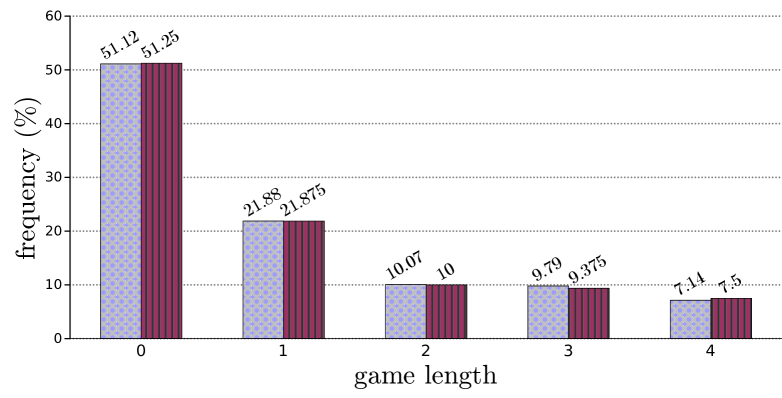
Figure 1: Comparison of simulated data (10,000 trial games) with analytic results from Table 5

In a follow-up paper to the present one—which has already appeared as [25]—we apply Proposition 4.1 and Theorem 4.2 to determine the game-length distribution in a long sequence of burn-off games on a complete graph. Thus we recover the corresponding enumeration results obtained by Cori, Dartois, and Rossin in [10]. These authors’ approach is through the (univariate) ‘avalanche polynomial’, which is, in our terminology, a generating function for the number of games of varying lengths. More recently, these polynomials were refined to their multivariate analogues in [1], where they are characterized for some basic graph families (trees, cycles, wheels, and complete graphs).

6 Concluding remarks

Early papers (e.g., [2], [3], [27]) that inspired the invention of the abelian sandpile model by Dhar [13] studied chip-firing games, in part, through computer simulations. Our first example in Section 5 is intended to illustrate how our main results (Theorem 3.1, Proposition 4.1, Theorem 4.2) offer an analytic explanation for the game-length distribution of a burn-off game, at least on the graph considered there. Though the two results from Section 4 do not offer closed-form expressions for the quantities being counted, the Matrix-Tree Theorem (see, e.g., [9]), together with Theorem 3.1, render as manageable the summands $t_{v}$ and $r(G-T)$ in Proposition 4.1 and Theorem 4.2. Thus, in principle, the exact probability distribution is available.

Closure

Somewhat out of sequence, this paper brings to an end our long-term project of producing a published account of the second author’s dissertation [23]. Besides the already mentioned articles [19] and [24], further results from [23] appear in [18] and [25]. As mentioned at the end of Section 5, the last of these cites the present paper; this is because it was written afterwards.

Acknowledgements

Most of the manuscript for this article was finalized while the first author was on sabbatical at the University of Otago in Dunedin, New Zealand. The author gratefully acknowledges the support of Otago’s Department of Mathematics and Statistics. Both authors thank the referees for the constructive suggestions (and promptness!).

References

- [1] D. Austin, M. Chambers, R. Funke, L. D. García Puente, and L. Keough. The multivariate avalanche polynomial. Australas. J. Combin., 72(3):421–445, 2018.
- [2] P. Bak and C. Tang. Earthquakes as a self-organized critical phenomenon. J. Geophys. Res., 94(B11):15635–15637, 1989.
- [3] P. Bak, C. Tang, and K. Wiesenfeld. Self-organized criticality: An explanation of the 1/f noise. Phys. Rev. Lett., 59:381–384, Jul 1987.
- [4] M. Baker and F. Shokrieh. Chip-firing games, potential theory on graphs, and spanning trees. J. Combin. Theory Ser. A, 120(1):164–182, 2013.
- [5] B. Benson, D. Chakrabarty, and P. Tetali. -parking functions, acyclic orientations and spanning trees. Discrete Math., 310(8):1340–1353, 2010.
- [6] N. Biggs and P. Winkler. Chip-firing and the chromatic polynomial. Research Report LSE-CDAM-97-03, Centre for Discrete and Applicable Mathematics, London School of Economics, London, U.K., 1997. 10pp.
- [7] N. L. Biggs. Chip-firing and the critical group of a graph. J. Algebraic Combin., 9(1):25–45, 1999.
- [8] A. Björner, L. Lovász, and P. W. Shor. Chip-firing games on graphs. European J. Combin., 12(4):283–291, 1991.
- [9] J. A. Bondy and U. S. R. Murty. Graph theory, volume 244 of Graduate Texts in Mathematics. Springer, New York, 2008.
- [10] R. Cori, A. Dartois, and D. Rossin. Avalanche polynomials of some families of graphs. In Mathematics and computer science. III, Trends Math., pages 81–94. Birkhäuser, Basel, 2004.
- [11] R. Cori and D. Rossin. On the sandpile group of dual graphs. European J. Combin., 21(4):447–459, 2000.
- [12] S. Corry and D. Perkinson. Divisors and sandpiles: An introduction to chip-firing. American Mathematical Society, Providence, RI, 2018.
- [13] D. Dhar. Self-organized critical state of sandpile automaton models. Phys. Rev. Lett., 64(14):1613–1616, 1990.
- [14] P. Diaconis and W. Fulton. A growth model, a game, an algebra, Lagrange inversion, and characteristic classes. Rend. Sem. Mat. Univ. Politec. Torino, 49(1):95–119 (1993), 1991. Commutative algebra and algebraic geometry, II (Italian) (Turin, 1990).
- [15] W. Feller. An introduction to probability theory and its applications. Vol. I. Third edition. John Wiley & Sons, Inc., New York-London-Sydney, 1968.
- [16] C. Godsil and G. Royle. Algebraic graph theory, volume 207 of Graduate Texts in Mathematics. Springer-Verlag, New York, 2001.
- [17] A. E. Holroyd, L. Levine, K. Mészáros, Y. Peres, J. Propp, and D. B. Wilson. Chip-firing and rotor-routing on directed graphs. In In and out of equilibrium. 2, volume 60 of Progr. Probab., pages 331–364. Birkhäuser, Basel, 2008. Corrected in arXiv:0801.3306v4 [math.CO], 20 June 2013.
- [18] P. M. Kayll and D. Perkins. Combinatorial proof of an Abel-type identity. J. Combin. Math. Combin. Comput., 70:33–40, 2009.
- [19] P. M. Kayll and D. Perkins. A chip-firing variation and a new proof of Cayley’s Formula. Discrete Math. Theor. Comput. Sci., 15(1):121–132, 2013.
- [20] C. J. Klivans. The mathematics of chip-firing. Discrete Mathematics and its Applications (Boca Raton). CRC Press, Boca Raton, FL, 2019.
- [21] L. Levine and J. Propp. What is a sandpile? Notices Amer. Math. Soc., 57(8):976–979, 2010.
- [22] C. Merino. The chip-firing game. Discrete Math., 302(1-3):188–210, 2005.
- [23] D. Perkins. Investigations of a chip-firing game. ProQuest LLC, Ann Arbor, MI, 2005. Thesis (Ph.D.)–University of Montana.
- [24] D. Perkins and P. M. Kayll. A chip-firing variation and a Markov chain with uniform stationary distribution. Australas. J. Combin., 68(3):330–345, 2017.
- [25] D. Perkins and P. M. Kayll. The length distribution for burn-off chip-firing games on complete graphs. Bull. Inst. Combin. Appl., 81:78–97, 2017.
- [26] D. Perkinson. Website: sandpiles. Available at people.reed.edu/davidp/sand/. Accessed 23 November 2019.
- [27] C. Tang and P. Bak. Mean field theory of self-organized critical phenomena. Journal of Statistical Physics, 51(5):797–802, 1988.
- [28] G. Tardos. Polynomial bound for a chip firing game on graphs. SIAM J. Discrete Math., 1(3):397–398, 1988.
- [29] J. van den Heuvel. Algorithmic aspects of a chip-firing game. Combin. Probab. Comput., 10(6):505–529, 2001.