Optimally controlled quantum discrimination and estimation

Abstract

Quantum discrimination and estimation are pivotal for many quantum technologies, and their performance depends on the optimal choice of probe state and measurement. Here we show that their performance can be further improved by suitably tailoring the pulses that make up the interferometer. Developing an optimal control framework and applying it to the discrimination and estimation of a magnetic field in the presence of noise, we find an increase in the overall achievable state distinguishability. Moreover, the maximum distinguishability can be stabilized for times that are more than an order of magnitude longer than the decoherence time.

I Introduction

Quantum control has become a very versatile tool for quantum technologies Glaser et al. (2015); Koch (2016), including quantum computation Palao and Kosloff (2003); Calarco et al. (2004); Goerz et al. (2011, 2017) and quantum simulation Cui et al. (2017); Omran et al. (2019). It is based on defining a figure of merit which quantifies how well the desired target is reached and which is taken to be a functional of yet unknown external fields Glaser et al. (2015); Koch (2016). Minimization, respectively maximization, of the functional yields pulse shapes for the external fields that drive the system to a target state or that implement a desired gate operation Glaser et al. (2015); Koch (2016). Various methods are now routinely being used to derive the pulse shapes, including both gradient-based optimization methods such as GRadient Ascent Pulse Engineering (GRAPE) Khaneja et al. (2005), Krotov’s method Palao and Kosloff (2003); Reich et al. (2012); Goerz et al. (2019), or the Gradient Optimization of Analytic conTrols (GOAT) algorithm Machnes et al. (2018), as well as gradient-free optimization such as the Chopped RAndom-Basis (CRAB) method Doria et al. (2011); Caneva et al. (2011).

The situation for applying quantum control, when compared with that in quantum computation or quantum simulation, is a bit different in quantum discrimination and quantum estimation, where the objective often does not involve a well-defined target state or gate Helstrom (1976); Holevo (1982); Yuen et al. (1975); Giovannetti et al. (2011, 2006); Braunstein et al. (1996); Fujiwara and Imai (2008); Escher et al. (2011); Demkowicz-Dobrzanski and Maccone (2014); Demkowicz-Dobrzanski et al. (2012); Huelga et al. (1997); Chin et al. (2012); Berry et al. (2015); Alipour et al. (2014); Beau and del Campo (2017); Liu et al. (2019); Tsang et al. (2016). For example, in quantum discrimination, the target is to distinguish a discrete set of quantum states or channels Helstrom (1976); Holevo (1982); Ogawa and Nagaoka (2000); Ogawa and Hayashi (2004); Hayashi (2002); Audenaert et al. (2007, 2008); Hiai and Petz (1991); Hayashi (2007); Acin (2001); D’Ariano et al. (2001); Duan et al. (2007); Lu et al. (2012); Chiribella et al. (2008); Duan et al. (2009); Harrow et al. (2010); Duan et al. (2008). Instead of driving the system to a fixed target, the control objective is to make the states more distinguishable to each other, since – intuitively – the error gets smaller when the states become more distinguishable. This is similar in quantum estimation Helstrom (1976); Holevo (1982); Yuen et al. (1975); Giovannetti et al. (2011, 2006); Braunstein et al. (1996); Fujiwara and Imai (2008); Escher et al. (2011); Demkowicz-Dobrzanski and Maccone (2014); Demkowicz-Dobrzanski et al. (2012); Huelga et al. (1997); Chin et al. (2012); Berry et al. (2015); Alipour et al. (2014); Beau and del Campo (2017); Liu et al. (2019); Tsang et al. (2016), where the task is to estimate the value of an unknown parameter encoded in the quantum dynamics. The error of the estimation gets smaller when the states evolved with different values of the parameter are more distinguishable.

Quantum discrimination and quantum estimation underlie many applications in quantum information science, including quantum hypothesis testing, quantum detection and quantum sensing. While quantum control has been employed to improve the precision in quantum estimation Yuan and Fung (2015); Yuan (2016); Xu et al. (2019); Liu and Yuan (2017a, b); Pang and Jordan (2017); Hou et al. (2019); Naghiloo et al. (2017); Predko et al. (2020); Mirkin et al. (2019), the use of quantum control in quantum discrimination remains scarce Childs et al. (2000); Chen and Yuan (2019); Van Damme et al. (2018). This is so despite the fact that one may expect quantum control to help identify fundamental performance bounds of quantum discrimination, similar to those found for quantum computation Caneva et al. (2009); Goerz et al. (2017), or derive pulse shapes for improved performance with direct relevance to experiments Omran et al. (2019); Larrouy et al. (2020). All that is required is to adapt the quantum optimal control toolbox to the specific use case of quantum discrimination.

Here, we develop a unified framework of optimal quantum control for quantum discrimination and quantum estimation. We employ the distance between two states that underwent different dynamics, more specifically that evolved under slightly different magnetic field strengths, as the figure of the merit. In the limit of the difference in field strength going to zero, optimizing this figure of merit becomes equivalent to optimizing the quantum Fisher information. We use quantum optimal control to maximize the distance between the two states by shaping the external fields that make up the interferometer. Intuitively, this can be understood as tailoring the external field to drive the states evolving under different dynamics away from each other, instead of towards a common target. Since both states depend on the control, the distance between them is typically not a linear function, which is different from the case of a fixed target. Krotov’s method for quantum optimal control Reich et al. (2012); Goerz et al. (2019) can be used in such a case. We employ it here to optimize discrimination and estimation of a magnetic field in the presence of noise, increasing the performance compared to the standard scheme based on a Ramsey interferometer. Our work thus contributes a quantum control perspective to current efforts for improving quantum sensing protocols based on Ramsey interferometry, using squeezed Schulte et al. (2020) or anticoherent Martin et al. (2019) states, variable detuning of the pulses Sadzak et al. (2019), or machine learning of the complete protocol Haine and Hope (2020).

The article is organized as follows. We introduce the figure of merit for discrimination and the estimation in Sec. II, and then present the quantum control method to optimize this figure of merit. In Sec. III, we apply the method to the discrimination and the estimation of the magnetic fields to demonstrate the feature and advantages of the control. We summarize our findings in Sec. IV.

II Model and Control Problem

We consider the dynamics described by the Gorini-Kossakowski-Sudarshan-Lindblad master equation Breuer and Petruccione (2002),

$$\frac{\mathrm{d}}{\mathrm{d}t}\mathsf{\rho}_{m}(t) =-\textup{i}\left[\mathsf{H}_{m}(t),\mathsf{\rho}_{m}(t)\right]$$

$$\quad+\sum_{k}\gamma_{k}\Big{(}\mathsf{L}_{k}\mathsf{\rho}_{m}(t)\mathsf{L}_{k}^{\dagger}-\frac{1}{2}\big{\{}\mathsf{L}_{k}^{\dagger}\mathsf{L}_{k},\mathsf{\rho}_{m}(t)\big{\}}\Big{)}$$

$$=\mathcal{L}_{m}(t)\mathsf{\rho}_{m}(t),$$ (1)

where

$$\mathsf{H}_{m}(t)=\mathsf{H}_{\mathrm{d},m}+\mathsf{H}_{\mathrm{c}}(t),$$ (2)

is the Hamiltonian. $\mathsf{H}_{\mathrm{d},m}$ describes the drift and $\mathsf{H}_{\mathrm{c}}(t)$ describes the coupling to an external drive, $\mathsf{L}_{k}$ are the Lindblad operators with the decay rates $\gamma_{k}$.

For quantum discrimination, we want to distinguish between two possible Hamiltonians, $\mathsf{H}_{\mathrm{d},1}$ and $\mathsf{H}_{\mathrm{d},2}$, while for quantum estimation, $\mathsf{H}_{\mathrm{d},m}$ depends on a continuous parameter which we want to estimate the value. In both cases $\mathsf{H}_{\mathrm{d},m}$ can not be measured directly, the discrimination (estimation) is achieved by the measurement of the time evolved state $\mathsf{\rho}_{m}(T)$ starting from an initial state $\mathsf{\rho}_{\mathrm{in}}=\ket{\Psi_{\mathrm{in}}}\bra{\Psi_{\mathrm{in}}}$. For the discrimination of two Hamiltonians, the two states $\mathsf{\rho}_{1}(T)$ or $\mathsf{\rho}_{2}(T)$ should be made as distinguishable as possible. In contrast, for the estimation the precision can also be connected to the distinguishability of the states that are evolved under two neighboring Hamiltonian with $\mathsf{H}_{\mathrm{d},1}=H(B-\delta B/2)$ and $\mathsf{H}_{\mathrm{d},2}=H(B+\delta B/2)$, where $\delta B$ is an infinitesimally small shift Braunstein and Caves (1994). The difference between the discrimination and the estimation is the figure of merit. The figure of merit for the discrimination is typically taken as the success probability $P_{\mathrm{succ}}$ to distinguish the two final states $\mathsf{\rho}_{1}(T)$ and $\mathsf{\rho}_{2}(T)$, which can be related to the trace distance $D_{\mathrm{tr}}$ as Helstrom (1976)

$$P_{\mathrm{succ}}=\frac{1}{2}\bigg{(}1+D_{\mathrm{tr}}\left(\rho_{1}(T),\rho_{2}(T)\right)\bigg{)}$$ (3)

where

$$D_{\mathrm{tr}}\left(\mathsf{\rho}_{1},\mathsf{\rho}_{2}\right)=\frac{1}{2}\left\lVert\mathsf{\rho}_{1}-\mathsf{\rho}_{2}\right\rVert_{\mathrm{tr}}\in[0,1],$$ (4)

$\left\lVert\mathsf{\rho}\right\rVert_{\mathrm{tr}}=\mathrm{Tr}\{\sqrt{\mathsf{\rho}^{\dagger}\mathsf{\rho}}\}$. The figure of merit for the estimation is typically taken as the precision, which can be calibrated by the quantum Cramer-Rao bound as $E[(\hat{B}-B)^{2}]\geq\frac{1}{R\mathcal{F}_{\mathrm{Q}}}$, where $E[(\hat{B}-B)^{2}]$ is the variance of an unbiased estimator $\hat{B}$, $R$ is the number of repetition of the experiments and $\mathcal{F}_{\mathrm{Q}}$ is the quantum Fisher information which determines the precision limit. Under the two Hamiltonian $\mathsf{H}_{\mathrm{d},1}=H(B-\delta B/2)$ and $\mathsf{H}_{\mathrm{d},2}=H(B+\delta B/2)$, the quantum Fisher information can be related to the Bures distance $D_{\mathrm{bures}}$ between $\mathsf{\rho}_{1}(T)$ and $\mathsf{\rho}_{2}(T)$ as Braunstein and Caves (1994)

$$\mathcal{F}_{\mathrm{Q}}=\frac{4D_{\mathrm{bures}}^{2}\left(\mathsf{\rho}_{1},\mathsf{\rho}_{2}\right)}{(\delta B)^{2}},$$ (5)

where the Bures distance between two states is defined as Jozsa (1994)

$$D_{\mathrm{bures}}^{2}\left(\mathsf{\rho}_{1},\mathsf{\rho}_{2}\right)=2-2\mathrm{Tr}\left\{\sqrt{\sqrt{\mathsf{\rho}_{1}}\mathsf{\rho}_{2}\sqrt{\mathsf{\rho}_{1}}}\right\}.$$ (6)

We consider distinguishing two Hamiltonians, $H_{\mathrm{d},1}=B_{1}\mathsf{\sigma}_{\mathrm{z}}/2$ and $H_{\mathrm{d},2}=B_{2}\mathsf{\sigma}_{\mathrm{z}}/2$. The discrimination of the two Hamiltonians can be related to the estimation when $B_{1}=B-\delta B/2$ and $B_{2}=B+\delta B/2$, which corresponds to the estimation of the strength of a magnetic field oriented along the $z$-axis.

We first compare two protocols for the discrimination — the standard Ramsey protocol and the protocol employing optimized control fields. Each protocol starts with preparing the qubit in the initial state $\mathsf{\rho}_{\mathrm{in}}=\ket{\Psi_{\mathrm{in}}}\bra{\Psi_{\mathrm{in}}}$ and is based on deducing whether the field is $B_{1}$ or $B_{2}$ by means of measuring its time-evolved state, $\mathsf{\rho}_{m}(T)$. The Ramsey scheme is to prepare an initial state on the Bloch sphere’s equator and let it subsequently evolve under the constant drift $\mathsf{H}_{\mathrm{d},m}$, i.e., $\mathsf{H}_{\mathrm{c}}(t)=0$. In contrast, the optimized protocol will in addition employ time-dependent fields, i.e., $\mathsf{H}_{\mathrm{c}}(t)\neq 0$. These control fields are optimized to make the two states $\mathsf{\rho}_{1}(T)$ and $\mathsf{\rho}_{2}(T)$ as distinguishable as possible. In other words, the optimized control fields need to maximize the distance measure $D(\mathsf{\rho}_{1},\mathsf{\rho}_{2})$. For the discrimination, the distance is the trace distance (4), since it is directly related to the successful probability of the discrimination, cf. Eq. (3). If expressed in terms of the Bloch vectors $\boldsymbol{r}_{1}$ and $\boldsymbol{r}_{2}$ for states $\mathsf{\rho}_{1}$ and $\mathsf{\rho}_{2}$, it reads $D_{\mathrm{tr}}\left(\mathsf{\rho}_{1},\mathsf{\rho}_{2}\right)=\lVert\boldsymbol{r}_{1}-\boldsymbol{r}_{2}\rVert/2$ with $\lVert\cdot\rVert$ the Euclidean vector norm Nielsen and Chuang (2011). Thus, the trace distance coincides with the geometric distance between the Bloch vectors $\boldsymbol{r}_{1}$ and $\boldsymbol{r}_{2}$ and maximal distinguishability is achieved iff $\boldsymbol{r}_{1}$ and $\boldsymbol{r}_{2}$ are on opposite points on the Bloch sphere. Hence, the maximization of $D_{\mathrm{tr}}$ will be our physical goal for the discrimination.

The presence of the drive Hamiltonian $\mathsf{H}_{\mathrm{c}}(t)$ allows to influence the evolution of $D_{\mathrm{tr}}$. We make the general assumption

$$\mathsf{H}_{\mathrm{c}}(t)=\frac{1}{2}\Big{[}\mathcal{E}_{\mathrm{x}}(t)\mathsf{\sigma}_{\mathrm{x}}+\mathcal{E}_{\mathrm{y}}(t)\mathsf{\sigma}_{\mathrm{y}}+\mathcal{E}_{\mathrm{z}}(t)\mathsf{\sigma}_{\mathrm{z}}\Big{]},$$ (7)

where $\mathcal{E}_{\mathrm{x}}(t),\mathcal{E}_{\mathrm{y}}(t),\mathcal{E}_{\mathrm{z}}(t)\in\mathbb{R}$ are control fields that couple via $\mathsf{\sigma}_{\mathrm{x}}$, $\mathsf{\sigma}_{\mathrm{y}}$ and $\mathsf{\sigma}_{\mathrm{z}}$ to the qubit, respectively. Note that while $\mathsf{H}_{\mathrm{c}}(t)$ is identical for both Hamiltonians $\mathsf{H}_{1}(t)$ and $\mathsf{H}_{2}(t)$, it influences the dynamics differently in the two cases due to the difference in the drift Hamiltonians. It can thus be used to maximize $D_{\mathrm{tr}}$. The presence of $\mathsf{H}_{\mathrm{c}}(t)$ thus turns the discrimination problem into a control problem, seeking to answer the question how to choose the three fields $\mathcal{E}_{\mathrm{x}}(t)$, $\mathcal{E}_{\mathrm{y}}(t)$ and $\mathcal{E}_{\mathrm{z}}(t)$ such that $D_{\mathrm{tr}}$ is maximized at time $T$ when the state $\mathsf{\rho}_{m}(T)$ is measured.

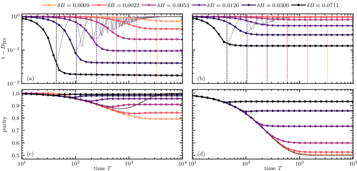
Figure 1: Improvement of the state distinguishability under the optimized control fields. The upper graphs show the indistinguishability $1-D_{\mathrm{HS}}$ as a function of protocol duration in case of (a) relaxation with $T_{1}=1000$ and (b) pure dephasing with $T_{2}=1000$. The dotted lines correspond to the Ramsey protocol whereas the markers indicates the reachable value of $1-D_{\mathrm{HS}}$ under the optimized control fields at the respective final time $T$. The vertical lines indicate the quantum speed limit given by Eq. (15). Panels (c) and (d) show the purity of the two states corresponding to the dynamics of panels (a) and (b), respectively. Note that both states have almost identical purity, hence there is just one visible solid line per $\delta B$ that indicates the purity of the final states under the optimized control fields.

We derive suitable control fields employing optimal control theory Glaser et al. (2015). To this end, we introduce the optimization functional

$$J\left[\left\{\mathsf{\rho}_{m}\right\},\left\{\mathcal{E}_{k}\right\}\right] =J_{T}\left[\left\{\mathsf{\rho}_{m}(T)\right\}\right]$$

$$\quad+\int_{0}^{T}\text{d}t\,g\left[\left\{\mathsf{\rho}_{m}(t)\right\},\left\{\mathcal{E}_{k}(t)\right\},t\right],$$ (8)

where $J_{T}$ is the relevant figure of merit that quantifies the failure probability or error at final time $T$ and $g$ captures additional running costs at intermediate times. The sets $\{\mathsf{\rho}_{m}\}$ and $\{\mathcal{E}_{k}\}$ are forward propagated states and control fields, respectively, here given by $\{\mathsf{\rho}_{1},\mathsf{\rho}_{2}\}$ and $\{\mathcal{E}_{\mathrm{x}},\mathcal{E}_{\mathrm{y}},\mathcal{E}_{\mathrm{z}}\}$. Equation (II) describes the most general form to represent an optimization functional and therefore constitutes the standard ansatz to formulate an optimization target D’Alessandro (2007). For the task of maximizing $D_{\mathrm{tr}}$, we choose $J_{T}$ as

$$J_{T}\left[\left\{\mathsf{\rho}_{1}(T),\mathsf{\rho}_{2}(T)\right\}\right] =1-D_{\mathrm{tr}}^{2}\left(\mathsf{\rho}_{1}(T),\mathsf{\rho}_{2}(T)\right)$$

$$=1-D_{\mathrm{HS}}\left(\mathsf{\rho}_{1}(T),\mathsf{\rho}_{2}(T)\right)$$ (9)

with $D_{\mathrm{HS}}$ the Hilbert-Schmidt distance Dodonov et al. (2000),

$$D_{\mathrm{HS}}\left(\mathsf{\rho}_{1},\mathsf{\rho}_{2}\right)=\frac{1}{2}\left\langle\mathsf{\rho}_{1}-\mathsf{\rho}_{2},\mathsf{\rho}_{1}-\mathsf{\rho}_{2}\right\rangle\in[0,1],$$ (10)

where $\langle\mathsf{A},\mathsf{B}\rangle=\mathrm{Tr}\{\mathsf{A}^{\dagger}\mathsf{B}\}$. Note that the relation $D_{\mathrm{tr}}^{2}=D_{\mathrm{HS}}$ only holds for qubits in which case maximization of $D_{\mathrm{tr}}$ and maximization of $D_{\mathrm{HS}}$ are equivalent. Since both distances are appropriate measures of state distinguishability, we choose $D_{\mathrm{HS}}$ for maximization in optimal control, since it is more suitable for that purpose Xu et al. (2004); Basilewitsch et al. (2019) because it allows to build analytical gradients with respect to the states $\mathsf{\rho}_{1}$ and $\mathsf{\rho}_{2}$.

In the following we briefly describe our numerical algorithm of choice. We use Krotov’s method Konnov and Krotov (1999), an iterative and gradient-based optimization technique, to minimize $J_{T}$, cf. Eq. (II). We achieve the minimization of $J_{T}$ by minimizing the total functional $J$, cf. Eq. (II), assuming $g$ to take the form Palao and Kosloff (2003)

$$g\left[\left\{\mathcal{E}_{\mathrm{x}}(t),\mathcal{E}_{\mathrm{y}}(t),\mathcal{E}_{\mathrm{z}}(t)\right\}\right]=\sum_{k=\mathrm{x},\mathrm{y},\mathrm{z}}\frac{\lambda_{k}}{S_{k}(t)}\left(\mathcal{E}_{k}(t)-\mathcal{E}_{k}^{\text{ref}}(t)\right)^{2},$$ (11)

where $\lambda_{k}$ is a numerical parameter, $S_{k}(t)\in(0,1]$ a shape function and $\mathcal{E}_{k}^{\text{ref}}(t)$ a reference field. Equation (11) is thereby a standard choice to control the pulse fluence and should prevent the optimization to optimize towards unphysical pulse shapes. With the choice of Eq. (11), Krotov’s method allows the derivation of a closed form for the field update Reich et al. (2012),

$$\mathcal{E}_{k}^{(i+1)}(t)=\mathcal{E}_{k}^{\mathrm{ref}}(t)+\frac{S_{k}(t)}{\lambda_{k}}\mathfrak{Re}\left\{\sum_{m}\Braket{\mathsf{\chi}^{(i)}_{m}(t)\;,\;\frac{\partial\mathcal{L}\left[\left\{\mathcal{E}_{k^{\prime}}\right\}\right]}{\partial\mathcal{E}_{k}}\Big{missing}}{{}_{\{\mathcal{E}^{(i+1)}_{k^{\prime}}(t)\}}\mathsf{\rho}^{(i+1)}_{m}(t)}\right\},$$ (12)

where the superscripts $(i)$ and $(i+1)$ indicate the previous and current iteration, respectively. The states $\mathsf{\rho}_{m}^{(i+1)}$ are determined by solving

$$\frac{\mathrm{d}}{\mathrm{d}t}\mathsf{\rho}^{(i+1)}_{m}(t) =\mathcal{L}^{(i+1)}(t)\mathsf{\rho}^{(i+1)}_{m}(t),$$ (13a)

$$\mathsf{\rho}^{(i+1)}_{m}(0) =\mathsf{\rho}_{\mathrm{in}}$$ (13b)

and the co-states $\mathsf{\chi}_{m}^{(i)}$ by solving

$$\frac{\mathrm{d}}{\mathrm{d}t}\mathsf{\chi}^{(i)}_{m}(t) =\mathcal{L}^{\dagger(i)}(t)\mathsf{\chi}^{(i)}_{m}(t),$$ (14a)

$$\mathsf{\chi}^{(i)}_{m}(T) =-\nabla_{\mathsf{\rho}_{m}(T)}J_{T}\big{|}_{\{\mathsf{\rho}^{(i)}_{m^{\prime}}(T)\}}.$$ (14b)

The superscripts of the Liouvillians $\mathcal{L}$, cf. Eq. (II), indicate the respective iteration of the control fields. The reference field in Eq. (12) is taken to be the field from the previous iteration, i.e., $\mathcal{E}_{k}^{\mathrm{ref}}(t)=\mathcal{E}_{k}^{(i)}(t)$. Hence, the running cost $g$ vanishes as the fields converge, and the total functional $J$ essentially coincides with the relevant figure of merit $J_{T}$ that we seek to minimize. See Ref. Reich et al. (2012) for a detailed description of Krotov’s method.

III Results and Discussion

The general time scale on which one can expect a given control task to be feasible is an important property of the dynamics. For instance, for a control problem where an initial state should be transferred into a given target state, it is determined by the general speed of the evolution, typically set by the Hamiltonian, and the distance between initial and target state. In our case, however, we are interested in the relative distance $D_{\mathrm{HS}}$ between the two time-evolved states $\mathsf{\rho}_{1}(t)$ and $\mathsf{\rho}_{2}(t)$ and not into their distance with respect to the initial state $\mathsf{\rho}_{\mathrm{in}}$. Hence, the time scale on which $D_{\mathrm{HS}}$ increases is defined by their relative speed of evolution. In detail, two different time scales are relevant for the problem of maximizing $D_{\mathrm{HS}}$. On the one hand, there is a quantum speed limit (QSL), i.e., a minimal time necessary to perfectly distinguish the two states. Such a minimal time is defined for every physical control task. Here, it is determined by $\delta B$ via the coherent part of the dynamics and can be estimated by

$$T_{\mathrm{QSL}}=\frac{\pi}{\delta B}.$$ (15)

This is the minimal time required for perfect state distinguishability, i.e., $D_{\mathrm{HS}}=1$, in the Ramsey protocol and under the assumption of no dissipation. On the other hand, dissipation continuously decreases $D_{\mathrm{HS}}$, since it causes both states, $\mathsf{\rho}_{1}(t)$ and $\mathsf{\rho}_{2}(t)$, evolving under $\mathsf{H}_{1}(t)$ and $\mathsf{H}_{2}(t)$ to evolve towards the same steady state $\mathsf{\rho}_{\mathrm{ss}}$. The time scale set by the dissipation is, in contrast to the QSL, independent of $\delta B$. Since the impact of relaxation and pure dephasing, characterized by $T_{1}$ and $T_{2}$, respectively, is quite different, we consider them individually in the following. This assumption is reasonable since in most physical settings, the noise is either $T_{1}$ or $T_{2}$ dominated. We take $\ket{\Psi_{\mathrm{in}}}=\ket{+}=(\ket{0}+\ket{1})/\sqrt{2}$ as initial state, in accordance with the standard Ramsey scheme Haroche and Raimond (2006), i.e., in our dynamical description, we do not account for the process preparing $\ket{\Psi_{\mathrm{in}}}$.

Figure 1 shows the distinguishability $D_{\mathrm{HS}}$ as a function of the protocol length $T$ for the Ramsey and optimized protocol. In detail, the dotted lines in Fig. 1(a) show the dynamics of $1-D_{\mathrm{HS}}$ for the Ramsey protocol, i.e., $\mathsf{H}_{\mathrm{c}}(t)=0$, for several $\delta B$ under relaxation, i.e., a single Lindblad operator $\mathsf{L}=\ket{0}\bra{1}$ with $\gamma=1/T_{1}$. The dashed vertical lines indicate the QSL of Eq. (15). Starting at $D_{\mathrm{HS}}=0$ at $T=0$, the distinguishability $D_{\mathrm{HS}}$ increases until it reaches the maximum of $D_{\mathrm{HS}}^{\mathrm{max}}$ at approximately $T\approx T_{\mathrm{QSL}}$. For times $T>T_{\mathrm{QSL}}$, the distinguishability $D_{\mathrm{HS}}$ decreases exponentially as the relaxation causes $\mathsf{\rho}_{1}(t)$ and $\mathsf{\rho}_{2}(t)$ to evolve towards the same ground/steady state $\mathsf{\rho}_{\mathrm{ss}}=\ket{0}\bra{0}$.

The decay of the state distinguishability due to relaxation can be completely suppressed by using tailored, i.e., optimized, control fields. The markers in Fig. 1(a) show the reachable distinguishability $D_{\mathrm{HS}}$ at the respective final time $T$ used in the optimization. There are two interesting effects to notice. On the one hand, the reachable maximum $D_{\mathrm{HS}}^{\mathrm{max}}$ increases compared to the Ramsey protocol. Hence, in the presence of relaxation, optimized control fields allow in general for better distinguishability despite a slightly longer protocol duration (factor $\lesssim 2$) to reach $D_{\mathrm{HS}}^{\mathrm{max}}$. On the other hand, the improvement in state distinguishability can be stabilized at that maximally reachable distance against decay for protocol durations $T$ much longer than the $T_{1}$ time. Figure 1(a) demonstrates it for times $T$ up to $10\times T_{1}$ but suggests it should, in principle, be feasible for even longer times.

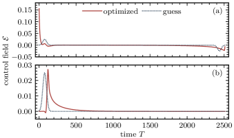
Figure 2: Guess (dotted) and unconstrained optimized (solid) field for the case of (a) relaxation with the control field $\mathcal{E}_{\mathrm{y}}(t)$ and (b) pure dephasing where the control is $\mathcal{E}_{\mathrm{x}}(t)$. The Bloch sphere dynamics is depicted in Figs. 3(a) and (b), respectively.

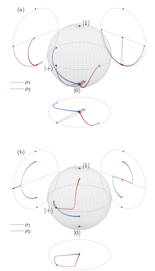
Figure 3: Exemplary dynamics of the two states $\mathsf{\rho}_{1}(t)$ and $\mathsf{\rho}_{2}(t)$ under the optimized fields within the Bloch sphere for (a) relaxation and (b) pure dephasing. The parameters are $\delta B=0.011$ with (a) $T_{1}=1000$ and (b) $T_{2}=1000$. The total time is $T=2511$ and the corresponding optimized fields are shown in Figs. 2(a) and (b). The density of dots on each line indicates the speed of the evolution with a low density corresponding to high speed and vice versa.

Figure 1(c) shows the purities for states $\mathsf{\rho}_{1}(t)$ and $\mathsf{\rho}_{2}(t)$ corresponding to the data in Fig. 1(a), both for the Ramsey protocol (dotted lines) and at final time $T$ after an evolution under the optimized control fields (markers). The dotted lines show an intermediate purity loss in the Ramsey protocol due to the relaxation. The final gain in purity for $t\rightarrow\infty$ is here a sign for the incoherent process of both states approaching the same (pure) ground/steady state. In contrast, the behavior of the purity in case of the improved and stabilized $D_{\mathrm{HS}}$ depends on $\delta B$. While for larger $\delta B$ the loss of purity is avoided at all $T$ by the respective optimized control fields, the improvement in case of small $\delta B$ comes along with a loss in purity.

The improvement and stabilization of $D_{\mathrm{HS}}$ is achieved via a simple control strategy which is most conveniently understood on the Bloch sphere, cf. Fig. 3(a). To this end, we choose the control field $\mathcal{E}_{\mathrm{z}}$ such that it cancels the known $B$, i.e., $\mathcal{E}_{\mathrm{z}}(t)=-B$. This eliminates the fast, coherent oscillations of $\boldsymbol{r}_{1}(t)$ and $\boldsymbol{r}_{2}(t)$ around the $z$-axis which do not contribute to the distinguishability $D_{\mathrm{HS}}$. Furthermore, in order to protect both states, $\boldsymbol{r}_{1}(t)$ and $\boldsymbol{r}_{2}(t)$, as much as possible from the detrimental relaxation, i.e., prevent their vector norms from shrinking, we kick both states from their initial position on the equator close to the ground/steady state $\mathsf{\rho}_{\mathrm{ss}}=\ket{0}\bra{0}$. This is achieved by a $\pi/2$ like pulse via $\mathcal{E}_{\mathrm{y}}$ right at the beginning of the protocol. The states will stay close to $\mathsf{\rho}_{\mathrm{ss}}$ for the largest part of the protocol where they evolve effectively decoherence-free in the vicinity of $\mathsf{\rho}_{\mathrm{ss}}$. For the final measurement both states are transferred back to the equator by a second, inverse $\pi/2$ like pulse.

Note that this strategy of protecting both states close to the ground/steady state for as long as possible has been identified in steps. Initially, we allowed the optimization of all three control fields $\mathcal{E}_{\mathrm{x}},\mathcal{E}_{\mathrm{y}},\mathcal{E}_{\mathrm{z}}$ and started optimizing without any strategic choice for their guess fields. However, the above strategy (with only slight deviations) has been identified even then. Its reduced version consists of a constant $\mathcal{E}_{\mathrm{z}}$ and no $\mathcal{E}_{\mathrm{x}}$ at all such that $\mathcal{E}_{\mathrm{y}}$ is the only time-dependent field that needs to be optimized.

Figure 2(a) shows, in an exemplary case, the guess and optimized form of $\mathcal{E}_{\mathrm{y}}(t)$ when guiding the optimization with a guess field that already incorporates the initial $\pi/2$ like kick in the beginning and its inverse counterpart at the end . Compared to the guess field, the optimization increases the intensity of the first kick such that the rotation from the initial equatorial state $\mathsf{\rho}_{\mathrm{in}}=\ket{+}\bra{+}$ towards $\mathsf{\rho}_{\mathrm{ss}}$ is carried out as fast as possible. The corresponding dynamics on the Bloch sphere is shown in Fig. 3(a). After the first kick, the states remain most of the time close to the ground/steady state $\mathsf{\rho}_{\mathrm{ss}}$, which effectively protects them from loosing purity. The second, inverse kick is much smoother and transfers the states symmetrically to the equatorial plane such that $D_{\mathrm{HS}}$ becomes maximal at $T$, i.e., the final time of measurement. The optimized field in Fig. 2(a) and its corresponding dynamics on the Bloch sphere, cf. Fig. 3(a), have been picked as a representative of an entire class of solutions for the problem of maximizing distinguishability in the presence of relaxation. The exact details of the optimized control field and corresponding dynamics differ depending on $\delta B$ and $T$, but the general control strategy remains similar.

We now turn to the case of pure dephasing with Lindblad operator $\mathsf{L}=\mathsf{\sigma}_{\mathrm{z}}$ and rate $\gamma=1/T_{2}$. Figure 1(b) shows the dynamics for the Ramsey protocol as dotted lines. In comparison to the case of $T_{1}$ decay, cf. Fig. 1(a), pure dephasing has a more severe influence on $D_{\mathrm{HS}}$ even if the decay rates are identical, $\gamma=1/T_{2}=1/T_{1}$. But also in this case, optimization is capable of improving $D_{\mathrm{HS}}$ over the Ramsey protocol — again at the expense of longer protocol durations (factor $\lesssim 2$). The effect of stabilizing $D_{\mathrm{HS}}$ at the maximal reachable distance for times much longer than the decay time can be observed as well. Nevertheless, the dynamics both in the Ramsey protocol as well as under the optimized control fields look quite different compared to relaxation. With pure dephasing no unique, single steady state exists but rather a set of states, namely the coherence-free states given by $\{\mathsf{\rho}_{\mathrm{ss}}=p\ket{0}\bra{0}+(1-p)\ket{1}\bra{1}|p\in[0,1]\}$, i.e., all states on the $z$-axis of the Bloch sphere. Since neither the drift $\mathsf{H}_{\mathrm{d},m}$ nor the dephasing cause a change of any state’s $z$-projection, the two states $\boldsymbol{r}_{1}(t)$ and $\boldsymbol{r}_{2}(t)$, starting initially in the equatorial plane, precess around the $z$-axis while loosing purity, i.e., shrink within the equatorial plane. Hence, they evolve towards the Bloch sphere’s center, i.e., the completely mixed state. This is evidenced by the dotted lines in Fig. 1(d), which show the purity evolving towards $1/2$ under the Ramsey protocol.

An optimization of all three available control fields $\mathcal{E}_{\mathrm{x}}$, $\mathcal{E}_{\mathrm{y}}$, $\mathcal{E}_{\mathrm{z}}$ again yields a simple control strategy. Like in the case of relaxation, it can also be realized by a single time-dependent control field, which is what for simplicity we discuss here. This time, the time-dependent control is $\mathcal{E}_{\mathrm{x}}(t)$, while $\mathcal{E}_{\mathrm{z}}(t)=-B$ again cancels the known field $B$ and $\mathcal{E}_{\mathrm{y}}$ is not needed at all. Figure 2(b) shows the guess field for $\mathcal{E}_{\mathrm{x}}(t)$, which exhibits a peak at the beginning. This peak is modified by the optimization such that it splits the two states $\boldsymbol{r}_{1}(t)$ and $\boldsymbol{r}_{2}(t)$ within the equatorial plane as a first step and then rotates them onto the $z$-axis in a second step, see Fig. 3(b) for the corresponding dynamics. Once the states reach the $z$-axis, $\mathcal{E}_{\mathrm{x}}(t)\approx 0$ is essentially turned off and the states become invariants of the dynamics which implies that their distinguishability $D_{\mathrm{HS}}$ can essentially be preserved forever. This readily explains the stabilization observed in Fig. 1(b). The respective optimized field and dynamics in Figs. 2(b) and 3(b) again represent an example for the entire class of solutions for the problem of maximal distinguishability in the case of pure dephasing. The exact details depend again on $\delta B$ and $T$.

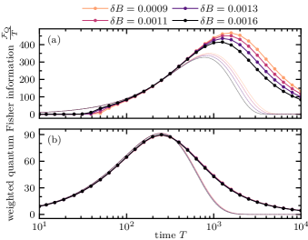
Figure 4: Quantum Fisher information $\mathcal{F}_{\mathrm{Q}}$ (weighted by the protocol duration $T$) for small values of $\delta B$. Panels (a) corresponds to the case of relaxation presented in Fig. 1(a) while panel (b) corresponds to the case of pure dephasing in Fig. 1(b). The dotted lines indicate the values for the Ramsey protocol whereas the markers show the optimized results.

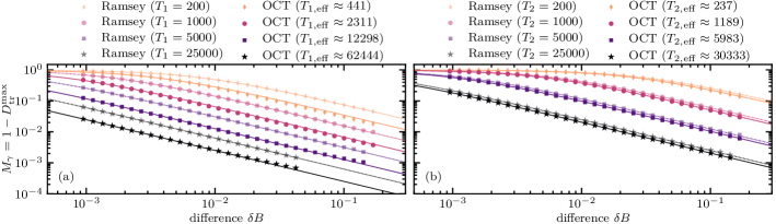
Figure 5: Improvement of the state distinguishability in terms of effective decay rates. The plot shows the maximal trace distance $D_{\mathrm{tr}}^{\mathrm{max}}$, i.e., minimal $M_{\gamma}$, as a function of $\delta B$ for several (a) relaxation and (b) dephasing times. The values for the Ramsey scheme (opaque markers) follow the analytical prediction of Eq. (III), shown as dotted lines. The non-opaque markers correspond to the optimized values of $D_{\mathrm{tr}}^{\mathrm{max}}$, i.e., numerical evaluation of Eq. (16). The solid lines are fits of the optimized values to Eq. (III) with fitting parameter (a) $\gamma=1/T_{1,\mathrm{eff}}$ and (b) $\gamma=4/T_{2,\mathrm{eff}}$.

Next, we relate the improved distinguishability $D_{\mathrm{HS}}$ observed in Fig. 1 to the quantum Fisher information $\mathcal{F}_{\mathrm{Q}}$, cf. Eq. (5). However, it depends on the Bures distance $D_{\mathrm{bures}}$, which is a distance metric on the set of density matrices, just as the trace distance $D_{\mathrm{tr}}$ or the Hilbert-Schmidt distance $D_{\mathrm{HS}}$. Unlike the trace distance discussed above, $D_{\mathrm{bures}}$ cannot be related to $D_{\mathrm{HS}}$, not even in the case of qubits. Nevertheless, the increase of $D_{\mathrm{HS}}$ is expected to increase $D_{\mathrm{bures}}$ as well Basilewitsch et al. (2019). For the maximization of $D_{\mathrm{HS}}$, shown in Fig. 1, this is in fact true and $D_{\mathrm{bures}}$ is readily improved alongside $D_{\mathrm{HS}}$.

Note that Eq. (5) is only valid for small $\delta B$. Moreover, it needs to be weighted by the protocol duration $T$ in order to quantify the amount of information that can be obtained per unit time for any given protocol. Accordingly, Fig. 4 shows the quantum Fisher information $\mathcal{F}_{\mathrm{Q}}$ weighted by the protocol duration for small values of $\delta B$. In the case of pure dephasing, cf. Fig. 4(b), there is a small improvement in $D_{\mathrm{HS}}$, respectively $D_{\mathrm{bures}}$, for the optimized protocol compared to the Ramsey protocol. This is, however, almost completely canceled by the slightly longer protocol duration $T$. As a result, the maximally reachable value of $\mathcal{F}_{\mathrm{Q}}/T$ is almost identical for the Ramsey and optimized protocols. In contrast, for relaxation, cf. Fig. 4(a), the significant improvement of $D_{\mathrm{HS}}$, respectively $D_{\mathrm{bures}}$, realized by the optimized protocol gives rise to an improvement of $\mathcal{F}_{\mathrm{Q}}/T$ despite the slightly longer protocol duration $T$. We thus expect a metrological gain of the optimized protocol compared to the Ramsey protocol.

So far, we only considered decay rates determined by $T_{1}=1000$ and $T_{2}=1000$. However, since the dissipation sets a time scale for the control task that is independent on the QSL set by $\delta B$, cf. Eq. (15), it is natural to ask whether the control strategy that has been identified above depends on the decay rates. To this end, we examine how the improvement of $D_{\mathrm{HS}}$, respectively $D_{\mathrm{tr}}=\sqrt{D_{\mathrm{HS}}}$, observed in Fig. 1 behaves for different relaxation and dephasing times. In detail, we are interested in the behavior of

$$M_{\gamma}(\delta B) \equiv\underset{t}{\mathrm{min}}\left\{1-D_{\mathrm{tr}}\left(\mathsf{\rho}_{1}(t),\mathsf{\rho}_{2}(t)\right)\right\},$$ (16)

as a function of $\delta B$ and for various decay rates $1/T_{1}$ and $1/T_{2}$. The function $M_{\gamma}$ measures, for a given $\delta B$, the maximally reachable distinguishability $D_{\mathrm{tr}}^{\mathrm{max}}$, independent of the time it takes to reach it. In other words, $M_{\gamma}(\delta B)=1-D_{\mathrm{tr}}^{\mathrm{max}}$. If, for a given physical process, the protocol duration is not crucial and only the maximally achievable state distinguishability is of importance, $M_{\gamma}(\delta B)$ is the relevant figure of merit. For the Ramsey protocol, Eq. (16) can be solved analytically to yield

$$M_{\gamma}(\delta B) =1-\Bigg{[}\frac{(\delta B)^{2}}{(\delta B)^{2}+\gamma^{2}}$$

$$\qquad\quad\times\exp\left\{-\frac{\gamma}{\delta B}\arccos\left(\frac{\gamma^{2}-(\delta B)^{2}}{\gamma^{2}+(\delta B)^{2}}\right)\right\}\Bigg{]}^{1/2}$$ (17)

for relaxation with $\gamma=1/T_{1}$. For pure dephasing, the solution takes the same form but differs by a factor of four, i.e., $\gamma=4/T_{2}$. The dotted lines in Figs. 5(a) and (b) show $M_{\gamma}$ for the Ramsey protocol for relaxation and pure dephasing, respectively. The dotted lines perfectly fit the numerical values given by the opaque markers, as expected for an analytical solution. For the dynamics under the optimized control fields, we can evaluate Eq. (16) numerically, cf. the non-opaque markers in Fig. 5. Remarkably, these show an almost identical functional dependence compared to the Ramsey scheme. We therefore fit the data obtained for the optimized protocol to Eq. (III) using effective relaxation and dephasing times as fitting parameters. This yields the solid lines in Fig. 5, which indeed show that $M_{\gamma}(\delta B)$ accurately describes the dependence also for the optimized data points with effective decay times $T_{1,\mathrm{eff}}$ or $T_{2,\mathrm{eff}}$, see the legends in Fig. 5. This is in fact not obvious as the coherent dynamics of the Ramsey and optimized protocol differ drastically, which makes the resemblance in their functional behavior of $M_{\gamma}$ remarkable. For relaxation, the effective decay times satisfy $T_{1,\mathrm{eff}}/T_{1}\approx 2.4$, whereas for pure dephasing, the ratio is $T_{2,\mathrm{eff}}/T_{2}\approx 1.2$. Thus, the maximally reachable distinguishability $D_{\mathrm{tr}}^{\mathrm{max}}$ behaves as though it would have been measured by a Ramsey protocol with $2.4$ times longer $T_{1}$, respectively $1.2$ times longer $T_{2}$ time, which greatly improves the distinguishability. Given the protection strategy of the dynamics, the prolongation of the decay times is not surprising, since the overall impact of the dissipation onto the states is reduced.

IV Conclusions

In summary, we have studied how optimized control fields can help to improve the distinguishability of two states of a qubit — both of which evolve under different drift but identical drive Hamiltonians while being exposed to either relaxation or pure dephasing. Our results show two improvements with respect to a standard Ramsey protocol for state discrimination.

First, optimized control fields increase the overall achievable state distinguishability, at the expense of slightly longer protocol durations. When comparing this improved state distinguishability against the prolonged protocol duration, in the case of relaxation, we observe a metrological gain, evidenced by the quantum Fisher information weighted by the protocol duration. In contrast, both effects — the improved state distinguishability and the prolonged protocol duration — roughly cancel in the case of pure dephasing.

Second, by utilizing optimize control fields, we are not only able to improve the state distinguishability but also to stabilize it at its maximum for times that are at least one order of magnitude longer than the decay times due to the environmental noise. The control strategy utilizes decoherence-free subspaces in all cases, where the states can be effectively stored and protected before being separated right before their measurement. We find the required control fields to be both simple and experimentally feasible.

Our study demonstrates the capabilities of optimal control to effectively reduce the environments detrimental influence. For the considered state discrimination problem and if compared to the standard Ramsey scheme, it reveals an alternative protocol with improved noise resistance. Our results thus suggest to explore state discrimination and its impact on quantum metrological applications from a new perspective.