Integration of max-stable processes and Bayesian model averaging to predict extreme climatic events in multi-model ensembles
ABSTRACT111Stochastic Environmental Research and Risk Assessment, 2019
Projections of changes in extreme climate are sometimes predicted by using multi-model
ensemble methods such as Bayesian model averaging (BMA) embedded with the
generalized extreme value (GEV) distribution. BMA
is a popular method for combining the forecasts of individual simulation models by
weighted averaging and characterizing the uncertainty induced by simulating the
model structure. This method is referred to as the GEV-embedded BMA. It is,
however, based on a point-wise analysis of extreme events, which means it overlooks the spatial dependency between nearby grid cells.
Instead of a point-wise model, a spatial extreme model such as the max-stable process
(MSP) is often employed to improve precision by considering spatial
dependency. We propose an approach that integrates the MSP into BMA, which is
referred to as the MSP-BMA herein. The superiority of the proposed method over the
GEV-embedded BMA is demonstrated by using extreme rainfall intensity data on the Korean peninsula from Coupled Model Intercomparison Project Phase 5
(CMIP5) multi-models. The reanalysis data called APHRODITE (Asian Precipitation Highly-Resolved
Observational Data Integration Towards Evaluation, v1101) and 17 CMIP5 models are
examined for 10 grid boxes in Korea.
In this example, the MSP-BMA achieves a variance reduction over the GEV-embedded BMA.
The bias inflation by MSP-BMA over the GEV-embedded BMA is also discussed.
A by-product technical advantage of the MSP-BMA
is that tedious ‘regridding’ is not required before and after the analysis while it should be done for the GEV-embedded BMA.
Keywords: Bias-variance trade-off; Bootstrap; Composite likelihood;
L-moments; Spatial extremes; Variance estimation
1. Introduction
The multi-model ensemble has the potential to combine the strengths of individual models and to better represent forecast uncertainty than the use of a single model. Various studies have shown the advantage of merging forecasts from multiple climate models for climate projection (e.g., Casey 1995; Coelho et al. 2004; Stephenson et al. 2005; Kharin et al. 2013; Arisido et al. 2017). A commonly used multi-model ensemble method is Bayesian model averaging (BMA), which assumes a probability distribution around the forecasts of individual models to establish the prior and uses a calibration period to determine the static weights for each individual model (Parrish et al., 2012; Wang et al., 2017).
When our interest is in forecasting extreme climatic events, the generalized extreme value distribution (GEVD) is typically used as an assumed probability distribution in BMA. The GEVD encompasses all three possible asymptotic extreme value distributions predicted by large sample theory (see, e.g., Leadbetter et al. 1983). It is widely used to analyze univariate extreme values (Coles, 2001). Zhu et al. (2013) performed a GEV-embedded BMA of extreme rainfall intensities by using seven regional climate models (RCMs). Hereafter, this method is referred to as the GEV-BMA. In that study, the method was applied to each grid cell separately; hence, it ignored the spatial dependency between nearby grid cells. Consequently, the GEV-BMA may be less reliable for small samples and could suffer from local fluctuations, which may be heavily influenced by outlier observations. Thus, it may be better to generalize this separate GEVD approach to a model taking into account the spatial dependency in the BMA framework. Therefore we consider a spatial extreme model, namely a max-stable process (see, e.g., de Haan 1984; Smith 1990; Davison et al. 2012). Max-stable process (MSP) is an infinite dimensional extension of the GEVD. The approach considered here, an MSP-embedded BMA, is a spatial extension of the GEV-BMA proposed by Zhu et al.(2013). Hereafter, the proposed method is referred to as the MSP-BMA.
MSPs are widely used for modeling spatial extremes, which deal with the spatial dependency of extreme events arising between nearby locations. The MSP estimates not only the GEVD parameters as continuous functions of space but also spatial dependent structure. The advantage of the MSP is that it can be used to address problems concerning the aggregation of global processes over many locations. Because it builds a model for the whole set of grid cells, it avoids local fluctuations that may be heavily influenced by outlier observations. Thus, more precise and robust return levels of extreme events can be obtained.
The present study aims to determine whether the integration of the MSP and BMA can add value when predicting future extreme values using multiple simulation models. It was motivated by Parrish et al. (2012) and Madadgar and Moradkhani (2014), who integrated data assimilation methods and copulas into BMA, respectively. Their results demonstrated that the predictive distributions after these integrations are more accurate and reliable, less biased, and more confident (i.e., having lower uncertainty). Sabourin et al. (2013) considered using BMA for multivariate extreme events. More recently, Najafi and Moradkhani (2015) and Yan and Moradkhani (2016) considered spatial hierarchical Bayesian modeling of extremes to obtain spatially distributed BMA weights corresponding to each simulation model. Our approach is in the same line of integrating spatial models into BMA framework. We are unaware of any work in which the MSP has been integrated into BMA. This is a reason why we considered MSP-embedded-BMA approach in this study. Based on the success of their research, we also expect a similarly good result by integrating the MSP and BMA.
To demonstrate the prediction ability of our approach, we use the annual maximum daily precipitation as simulated by Coupled Model Intercomparison Project Phase 5 (CMIP5) models in historical and future experiments over the Korean peninsula. Based on the variance estimates of return levels and other criteria, our approach seems outperforming the GEV-BMA.
The remainder of this paper is organized as follows. Section 2 describes models of extreme events including the GEVD and the MSP. Section 3 explains the GEV-embedded BMA and introduces the integrated MSP-BMA. Section 4 provides a numerical study of extreme rainfall as simulated by CMIP5 models over the Korean peninsula. A computationally faster version of the MSP-BMA is considered in Section 5. Section 6 concludes with discussion.
2. Modeling extreme values
2.1 Extreme value distribution
The GEVD is widely used to analyse univariate extreme values. The three types of extreme value distributions are sub-classes of GEVD. The cumulative distribution function of the GEVD is as follows:
| (1) |
when , where , and are the location, scale, and shape parameters, respectively. The particular case for in Eq. (1) is the Gumbel distribution, whereas the cases for and are known as the Fréchet and the negative Weibull distributions, respectively ([6]).
Assuming the data, the annual maxima of daily precipitation in this study, follow (approximately) a GEV distribution, the parameters can be estimated by using the maximum likelihood method (see, e.g., Wilks 1995 or Coles 2001) or the method of L-moments estimation (Hosking, 1990). The maximum likelihood estimator is less efficient than the L-moments estimator in small samples for typical shape parameter values (Hosking et al. 1985). The L-moments method is used in this study because relatively short 30-year samples are analyzed for each comparison period. Moreover, the formulae used to obtain the L-moments estimator are simple compared with obtaining the maximum likelihood estimator, which needs an iterative computation until convergence. Those are
| (2) |
where
| (3) |
and and are the sample second and third L-moments (Hosking, 1990). The other parameters are then given by
| (4) |
| (5) |
where is the first sample L-moment.
It can be helpful to describe changes in extremes in terms of changes in extreme quantiles. These are obtained by inverting (1):
| (6) |
where . Here, is known as the return level associated with the return period , since the level is expected to be exceeded on average once every years (Coles, 2001). For example, a 20-year (50-year) return level is computed as the 95th (98th) quantile of the fitted GEVD. This return level is used as the main quantity in the numerical study to compare the GEV-BMA with the MSP-BMA in the subsequent sections.
2.2 Models for spatial extremes
Extreme value distributions are typically applied independently for the datasets of each weather station (grid cell, in this study). However, a better approach may be to build a model for all the weather stations together to avoid local fluctuations and reflect the spatial dependency between observations from nearby stations. A variety of statistical tools have been used for the spatial modeling of extremes including Bayesian hierarchical models, copulas and max-stable processes. The first model is often referred to as “latent variable” approach (Davision et al., 2012).
Spatial hierarchical models introduce spatial variation in the parameters of the extremal response distributions. By letting the parameters of the response distributions depend on the unobserved latent processes, the spatial hierarchical model induces dependence in responses by integration over the latent process. A Gaussian process is frequently used for the latent process. This approach is common in geostatistics with nonnormal response variables (Diggle and Ribeiro, 2007), and because of the complexity of the integration involved is most naturally performed in a Bayesian setting, using Markov chain Monte Carlo algorithms to perform inferences (see, e.g., Sang and Gelfand, 2010; Cooley et al., 2012; Fawcett and Walshaw, 2016). Compared to the models based on copulas and MSP, it is reported that the spatial hierarchical modeling makes quantifying uncertainty more straightforward, and it allows a better fit to marginal distribution, but it fits the joint distributions of extremes poorly (Davision et al., 2012).
Copula provides a unifying framework to modeling multivariate data, and so may be useful to model spatial extremes. Given marginal GEVDs and some correlation functions, various copulas including Gaussian and Student t are available. Some copulas satisfying the max-stability property, called as extremal copulas, may be useful to model spatial extremes (see, e.g., Nelsen 2006; Salvadori and De Michele 2004; Madadgar and Moradkhani 2014; Requena et al. 2016).
The max-stable processes (MSP) is an useful natural extension of the extremal (univariate and multivariate GEV) models. It is an infinite-dimensional generalization of the univariate GEV model, and is particularly applicable in the context of a time series or a spatial process. This theory was introduced by De Haan (1984) and has been extended by a number of researchers such as Smith (1990), Schlather (2002), Kabluchko et al. (2009), and Padoan et al. (2010). Appropriately chosen max-stable models seem essential for successful spatial modeling of extremes (Davision et al., 2012). It, however, also bring challenges. For example, the likelihood is hard to tractable for even moderate sample size problems, and consequently composite (or pairwise) likelihood methods are utilized.
For future projections and uncertainty assessment of extreme events from an ensemble of climate models, many proposed the integration of spatial extreme models and BMA framework. We are, however, unaware of any work in which the MSP has been integrated into BMA. Thus we propose an integration of MSP and BMA in multi-model ensemble, in this study.
2.3 Max-stable processes
The max-stable process (MSP) is defined as the limit process of the maxima of the independent and identically distributed random fields (De Haan, 1984) and can be expressed as
| (7) |
if a limit exists for all in with normalizing constants and . For a fixed point () in space, any d-dimensional marginal distribution of the MSP belongs to a class of multivariate extreme value distributions. In practice, this means that the resulting parameters , and are the continuous functions to be estimated. Thus, the MSP naturally permits modeling and predictions with data-level spatial dependence. We then build the regression-based forms for the parameters and estimate the spatial dependence parameters ([48]). These regression-based forms, however, may introduce some estimation bias for MSP while it are convenient to predict something for non-observed sites.
The precision of the estimated parameters in the MSP is expected to be improved over the point-wise (or at-site) GEV model because the MSP allows more data to be used in the model fitting by combining data from multiple sites across a spatial domain (Ribatet, 2013; Gaume et al., 2013; and Oesting and Stein, 2017).
Given a series of observations at spatial locations, the aim of a statistical analysis would be to fit an MSP by using assumed forms for the parameters , and , while also estimating spatial dependence. However, for more than spatial locations, the distribution function of the general MSP has no analytically tractable form, which thereby presents a problem for practical statistical model fitting. Therefore, ad hoc characterization methods have been proposed. Smith (1990) introduced the first, and Schlather (2002) and Kabluchko et al. (2009) later introduced other methods. Schlather’s characterization involves a correlation function , deriving a bivariate cumulative distribution function as
| (8) | |||
| (9) |
where is the distance between and . Further, , where the lower bound corresponds to the independence of extremes. To take into account the spatial dependency, we used a powered exponential correlation function of distance , in this study [8]:
| (10) |
where and are the scale and shape parameters that control the range and smoothness of the process, respectively. The Brown–Resnick model [20] uses the following variogram [8]:
| (11) |
The full likelihood of the MSP is often analytically unknown or computationally prohibitive to calculate. The following pair-wise log likelihood function is used because only the bivariate density function is specified;
| (12) |
where is the -th observation at the -th site for . The use of the pair-wise likelihood method leads to an underspecified model. Thus, instead of the Akaike information criterion, the Takeuchi information criterion (TIC) is used to select a better model for the estimated parameters [44]:
| (13) |
where stands for the trace of matrix A, and
| (14) |
where means the derivative with respect to . A model with a low TIC is a good one.
3. Bayesian model averaging for extreme events
3.1 Bayesian model averaging using GEV distribution
Over the past few decades, ensemble forecasts based on global climate models have become an important part of climate forecasting because of their ability to reduce prediction uncertainty. Among the various ensemble methods, BMA combines the forecast distributions of different models and builds a weighted predictive distribution from them. Many empirical studies including Raftery et al. (2005), Sloughter et al. (2007), Wang et al. (2012), Mok et al. (2018), and Huo et al. (2018) have shown that various BMA approaches outperform other competitors in prediction performance. To calculate the weight of each forecast model, Raftery et al. (2005) used the expectation maximization algorithm and estimated the weights based on the performance of each model during a training period.
In standard BMA, the conditional distribution of each individual model is assumed to follow a normal distribution, which is valid for temperature and sea-level pressure, for example. For other variables such as maximum precipitation or extreme wind speed, the GEVD might be a better alternative for representing the distribution of the model’s output. In their climate change study of extreme rainfall, Zhu et al. (2013) used the GEVD in a BMA framework, where the weight of each forecast model was calculated by comparing the reanalysis data with the historical data from a simulation model. Moreover they applied the bootstrap technique instead of employing the expectation maximization algorithm to compute the weights of the models and variance of the BMA predictions of rainfall intensity. Now, we describe the details of their method, which is referred to as the GEV-BMA in this paper.
Given the relatively short record of 30 years from the climate model and reanalysis data in this study, the parameter estimation of the GEVD may be imprecise and problematic for predicting events beyond the range of the observed data (e.g., return level for 100 years). Thus, Zhu et al. (2013) proposed a bootstrap-based approach to establish the uncertainty of the prediction. Based on the ability of each climate model’s historical runs in matching the reanalysis data for each location, the weights for all RCMs were calculated. For each RCM and each bootstrap realization, the GEV parameters were generated and rainfall intensity (i.e., return level) in return period T estimated. The variance in rainfall intensity was calculated for all bootstrap realizations (from i=1 to B). They then used the Gaussian likelihood function as follows:
| (15) |
where is the intensity of the i-th bootstrap from the reanalysis data, is the intensity of the i-th bootstrap from the historical data of model , and
| (16) |
is the variance in intensity based on the reanalysis data, where . Note that the data from all models were downscaled to have the same grids as the reanalysis data in advance of fitting the GEVD at each site.
If is the rainfall intensity of return period predicted by a set of K alternative models, then its distribution conditioned on the reanalysis data R is (Hoeting et al., 1999)
| (17) |
where is the predictive probability of for model and is the posterior probability of . One way of estimating the posterior model probability is to use Bayes’ theorem:
| (18) |
where is the likelihood of model and is the prior probability of . The above quantity (18) is used as the weights of the BMA as in the below equation (20). Here, may be assigned based on prior information from expert elicitation, professional assessments of the incorporated models, and so on. If such information is unavailable, the prior probabilities could be set to be equal for all the models. In the numerical study of this article, equal priors are used for all 17 models. The likelihood of model is approximated by using the generalized likelihood uncertainty estimation method (Beven, 2006; Rojas et al., 2008):
| (19) |
The mean and variance of the BMA prediction of rainfall intensity over models are then given by
| (20) |
| (21) |
where is the weight for each model . For the historic data, these quantities are estimated by the calculation from the bootstrap samples used in (15):
| (22) |
and
| (23) |
For the future simulation data, the above equations (22) and (23) are not used, but the intensity estimates obtained by fitting GEVDs to each model’s future data are used. That is, , where the subscript stands for the future data. For estimation of , we may need to consider other quantities such as asymptotic variance.
3.2 Bayesian model averaging using MSP
In Zhu et al. (2013), the dataset from a simulation model in each grid point was treated independently even though nearby observations were aggregated. That is, the GEVD was fitted at-site and the return levels in period T were estimated for each grid. The weighted average of these return levels over a suite of simulation models is the GEV-BMA prediction. As mentioned in subsection 2.3, the precision of these estimated return levels can be improved by applying the MSP instead of using point-wise GEV models. Now, we propose an integration of BMA and the MSP with the expectation of an improved ensemble prediction compared with the GEV-BMA. We refer to this new integrated approach as the MSP-BMA.
In the MSP-BMA, the MSPs are fitted to the reanalysis data and the historical data of model , respectively, over the spatial domain. Then, the return level, , at each site is obtained by using the following equation:
| (24) |
where . This is a spatial extension of equation (6). Here, the GEV parameters obtained from the MSP fitting are functions of the spatial variables given in (27) in the next section. To compute (15), bootstrap samples are used as in the GEV-BMA. These are obtained by random sampling with replacement over the spatial domain, from the reanalysis data and the historical data of model . It was sampled ‘year-wise’ over spatial stations. If the year 1980 is selected, for example, then the observation vector of all stations on the year is used as a bootstrap realization. Then, the BMA weights are calculated by using the same formula as in (18). Moreover, the BMA prediction and uncertainty estimates over multi-models for the future data are calculated by the same equations as in (20) and (21), respectively.
The main advantage of the MSP-BMA is that the precision of the BMA prediction is improved, as shown by the illustrative numerical study in the next section. As an advantage of MSP-BMA as a by-product, we have experienced a technical convenience of handling data in applying MSP-BMA to multiple climate models compared to applying GEV-BMA. It is because that each climate model has different resolution and so has different locations and sizes of grid cells. Moreover, those are also different from those of reanalysis data. Thus, to compare each model to reanalysis data and to combine multi-models, we needed a pre-processing to make the center points of grid cells to be same (i.e., regridding) across multi-models and reanalysis data in applying GEV-BMA, while we do not need it in applying MSP-BMA.
3.3 Comparison methods
To compare the performances of the GEV-BMA and the MSP-BMA, we considered the following two criteria. The first one is the quantile per quantile (qq) plot for the group-wise maxima to check the goodness-of-fit (Davison and Gholamrezaee, 2012). Here, the empirical group-wise maxima for each year are selected from the given observations across the sites, while the theoretical group-wise maxima are obtained from the average of the randomly generated MSPs for each year. This is done for all the years (30 years in this study) to construct a maxima series. Then, the quantiles from each maxima series are plotted. This plot with a confidence band is drawn for each method and compared.
The second criterion is the variance in return levels of each method for each site. This is calculated by using equation (23) for both methods. Lower variance values represent less uncertainty in the estimation. This comparison is conducted for each site (10 locations in this study). The relative improvement is calculated by
| (25) |
4. Numerical study
4.1 Datasets
We analyze annual maximum daily precipitation (AMP1) as simulated by the CMIP5 models in the historical experiments (1971–2000) and the experiments for the 21st century (2021–2050). We considered the models only employing one radiative forcing scenario, called Representative Concentration Pathways (RCP) 4.5. Table 1 lists the model names, institutes, and resolution of the 17 models considered in this study.
For the reanalysis data, we use APHRODITE (Asian Precipitation Highly-Resolved Observational Data Integration Towards Evaluation, v1101) daily gridded precipitation data. This is the long-term (1951 onward) continental-scale daily product that contains a dense network of daily rain-gauge data for Asia including the Himalayas, South and Southeast Asia, and mountainous areas in the Middle East (Yatagai et al., 2009). The grid resolution of APHRODITE is for East Asia including Korea. We treat this reanalysis data as the “ground truth.”
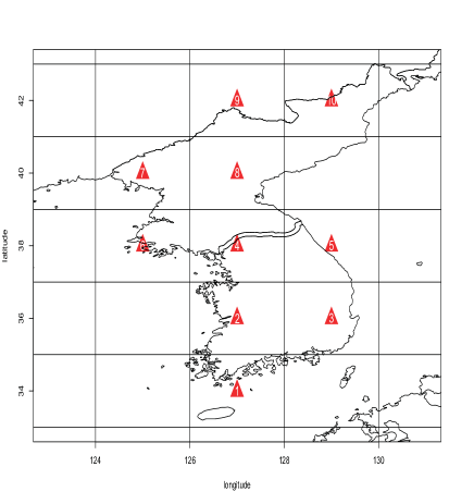
In a statistical analysis such as the GEV-BMA, we need to match the grid point of the reanalysis data to that of the CMIP5 models. However, the resolution of the CMIP5 models varies, as seen in Table 1, and thus we need a standard grid to efficiently use these datasets. For such a standard grid, we set the grids as , as seen in Figure 1. For each box in the figure, there are 16 observations of AMP1 from APHRODITE. We treat the average of these 16 observations as the representative AMP1 of the grid box. For our study, 10 boxes are chosen over the Korean peninsula. The red triangle in Figure 1 stands for the center site of the box. For each site, a time series of 30 years (from 1971 to 2000) AMP1 is used. For the historical and future data from each simulation model, the Kriging method is applied to obtain the observation (AMP1) at the center site. The “DiceKriging” package in R software (Roustant et al., 2012) was used with Matern 5/2 covariance structure. Now, we have three kinds of datasets for each site: reanalysis and historical data from 1971 to 2000 (period 0) and future simulation data from 2021 to 2050 (period 1).
| Model Name | Institution | Resolution |
|---|---|---|
| (LonLat Level#) | ||
| BCC-CSM1-1 | Beijing Climate Center, China Meteorological Ad- | 192145L38 |
| ministration, China | ||
| CanESM2 | Canadian Centre for Climate Modelling and Anal- | 12864L35(T63) |
| ysis | ||
| CCSM4 | National Center for Atmospheric Research(NCAR), | 288192L26 |
| USA | ||
| CNRM-CM5 | Centre National de Recherches Meteorologiques, | 256128L31(T127) |
| Meteo-France | ||
| GFDL-ESM2G | Geophysical Fluid Dynamics Laboratory, USA | 14490L24 |
| GFDL-ESM2M | Geophysical Fluid Dynamics Laboratory, USA | 14490L24 |
| HadGEM2-AO | National Institute of Meteorological Research/ | 192145L40 |
| Korea Meteorological Administration, Korea | ||
| HadGEM2-CC | UK Met Office Hadley Centre | 192145L40 |
| HadGEM2-ES | UK Met Office Hadley Centre | 192145L40 |
| INMCM4 | Institute for Numerical Mathematics, Russia | 180120L21 |
| IPSL-CM5A-LR | Institute for Pierre-Simon Laplace, France | 9696L39 |
| MIROC5 | Model for Interdisciplinary Research on Climate, | 256128L40(T85) |
| Japan | ||
| MIROC-ESM | Model for Interdisciplinary Research on Climate, | 12864L80(T42) |
| Japan | ||
| MIROC-ESM- | Model for Interdisciplinary Research on Climate, | 12864L80(T42) |
| CHEM | Japan | |
| MPI-ESM-LR | Max Planck Institute for Meteorology, Germany | 19296L47(T63) |
| MRI-CGCM3 | Meteorological Research Institute, Japan | 320160L48(T159) |
| NorESM1-M | Norwegian Climate Centre, Norway | 14496L26 |
4.2 MSP modeling
For the data analysis, we employ a linear transformation to make the station’s geographical information be in [0, 1]:
| (26) |
This makes the calculation of the inverse of the Hessian matrix more stable. According to the data, the minimum and maximum values of the latitudes, longitudes, and altitudes are (34.23, 38.15) degrees, (126.22, 129.24) degrees, and (1.3m, 263.1m), respectively. To compute the MSP, we use the R package “SpatialExtremes” developed by Ribatet et al. (2013).
From the reanalysis data, we build regression-based forms to the location and scale parameters by including latitude and longitude, where denotes the station. We set as a constant , which is typical in MSP modeling (Buishand et al., 2008; Westra and Sisson, 2011; Lee et al., 2013), because we are studying with a small number of grid cells. The selected model at the minimum of the TIC is as follows:
| (27) | |||||
where and are the latitude and longitude of the site and , , are the regression coefficients corresponding to the variables. This selected regression form is fixed for the MSP for the historical and future data in this study because the model selection based on the TIC for the 17 CMIP5 models took huge computing time. However, the regression coefficients are estimated for every dataset by maximizing the pair-wise log likelihood function given in (12). Here it is notable, as commented by a reviewer, that the polynomial form for GEV parameters is just a convenience assumption but may not be very flexible. Treating GEV parameters as Gaussian processes in spatial Bayesian hierarchical model may provide a more flexible alternative.
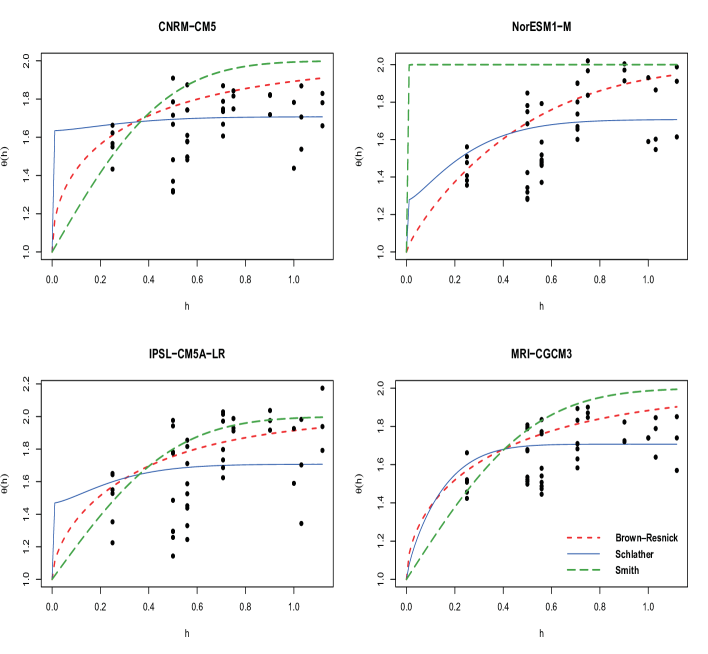
To select the characterization among the three approaches (Smith, Schlather, and Brown–Resnick), we check the extremal coefficient plots for each simulation model. Figure 2 shows typical plots drawn for some of the simulation models: CNRM-CM5, NorESM1-M, IPSL-CM5A-LR, and MRI-CGCM3. From these plots, we choose the Brown–Resnick characterization in this study.
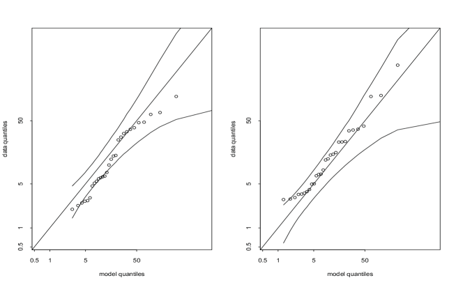
Figure 3 shows the group-wise maxima qq plots. The left panel is from the GEV fitting and the right one is from the MSP fitting to the reanalysis data. The right plot provides a better qq than the left one in the sense that the points in the right plot are closer to the straight line and more located inside the confidence band. This means that the MSP is more acceptable than the GEVD for this dataset.
4.3 BMA result for comparison
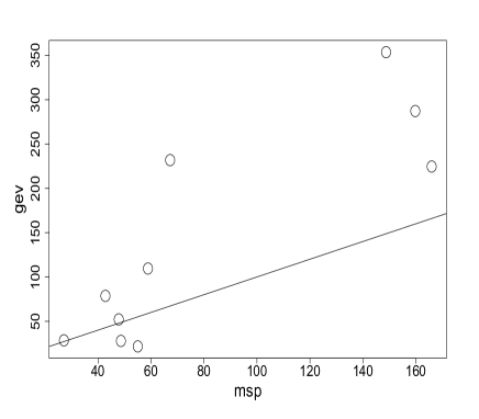
For each site, the variance estimates of the 20-year return levels are calculated from the GEV-BMA and the MSP-BMA by using the reanalysis and historical data. Figure 4 compares these two kinds of variances (unit: ). The Y-axes and X-axes stand for the variances estimated by using the GEV-BMA and the MSP-BMA, respectively. The GEV-BMA has greater variance than the MSP-BMA for eight of the 10 sites. This may mean that the MSP-BMA provides more precise predictions with less uncertainty than the GEV-BMA. Table 2 shows the estimated variances of the 20-year return levels obtained by using both BMA methods. The relative improvement is calculated by the formula (25) in which the MSP-BMA achieves a 42% relative variance reduction on average over the GEV-BMA.
| Site | Var(GEV-BMA) | Var(MSP-BMA) | Relative Improvement(%) |
|---|---|---|---|
| 1 | 353.6 | 148.7 | 57.9 |
| 2 | 109.5 | 58.9 | 46.3 |
| 3 | 224.6 | 166.0 | 26.1 |
| 4 | 231.8 | 67.2 | 71.0 |
| 5 | 287.2 | 159.8 | 44.4 |
| 6 | 78.6 | 42.8 | 45.6 |
| 7 | 27.8 | 48.6 | -74.9 |
| 8 | 21.6 | 55.0 | -154.3 |
| 9 | 28.5 | 27.1 | 4.8 |
| 10 | 52.1 | 47.8 | 8.3 |
| Average | 141.5 | 82.2 | 41.9 |
It may not be surprise that the variances obtained from MSP is smaller than point-wise GEV, but it could also due to the spatial modeling bias and the variance estimation may be too small to be true. Thus we used a bootstrap method to estimate the bias more reasonably. Bootstrap samples are obtained by random sampling with replacement over the spatial domain, from the reanalysis data and the historical data of model . It was sampled ‘year-wise’ over spatial stations, as we did in the previous section 3.2. The bias is calculated by the difference between the true 20-year return level and estimated levels obtained by a bootstrap sample. This calculation is repeated times, and the average of differences is considered to be the bias of the model. Here, for the true 20-year return level, we used the estimate of 20-year return level obtained by applying GEV-BMA model for the original data. If we set the true 20-year return level differently from this study, the bias estimates for both models may be changed. The table 3 shows the bias estimates calculated by using GEV-BMA and MSP-BMA methods. The table shows that the MSP-BMA has bias inflation over GEV-BMA at eight sites. The bias of MSP-BMA may be introduced by assuming a regression model for each GEV parameter. By considering both results from Tables 2 and 3, we know that it is an example of bias-variance trade-off problem, as commented by a reviewer. We leave more study on this matter to future work.
| Site | Bias(GEV-BMA) | Bias(MSP-BMA) |
|---|---|---|
| 1 | 30.5 | 33.1 |
| 2 | 13.9 | 17.6 |
| 3 | 15.3 | 13.4 |
| 4 | -14.4 | -15.7 |
| 5 | 25.2 | 27.7 |
| 6 | 18.4 | 28.3 |
| 7 | -7.5 | -10.8 |
| 8 | -10.9 | -20.1 |
| 9 | 1.1 | -8.2 |
| 10 | -11.2 | -10.7 |
5. Summary and discussion
In this study, a MSP-embedded BMA is proposed to project extreme climates based on multi-model ensemble simulations. The proposed method, referred to as the MSP-BMA, is a spatial extension of BMA embedded with a point-wise GEVD. The superiority of the proposed method over the GEV-embedded BMA is demonstrated by using extreme rainfall intensity data on the Korean peninsula from CMIP5 multi-models. The APHRODITE reanalysis data and 17 CMIP5 models are examined for 10 grid boxes over the Korean peninsula.
A conclusion of this study is that the MSP-BMA outperforms the GEV-embedded BMA by generating lower prediction variance estimates for extreme rainfall intensity data on the Korean peninsula. The MSP-BMA achieves a 42% relative variance reduction over the GEV-embedded BMA on average. However, the regression-based forms in MSP may introduce some bias, which needs more study on this bias-variance trade-off problem.
A by-product technical advantage of the MSP-BMA is that tedious ‘regridding’ is not required before and after the analysis while it should be done for the GEV-embedded BMA.
As commented by a reviewer, the constant parameter assumption in MSP effectively reduces the estimation uncertainty while there is no such a constraint from point-wise GEV method. For a fair comparison, one can also modify the point-wise GEV method to a constant shape parameter GEV model (Wang et al. 2016). We leave this matter to future work.
Acknowledgment
The authors would like to thank two reviewers and Associate Editor for their valuable comments and constructive suggestions. This work was supported by the National Research Foundation of Korea (NRF) grant funded by the Korean government (No.2016R1A2B4014518), and also funded by the Korea Meteorological Administration Research and Development Program under Grant KMI2018-03414. Lee’s work was supported by the Basic Science Research Program through the NRF funded by the Ministry of Education (2017R1A6A3A11032852).
References
- Arisido et al. [2017] Arisido, M.W., Gaetan, C., Zanchettin, D. et al. A Bayesian hierarchical approach for spatial analysis of climate model bias in multi-model ensembles. Stoch Environ Res Risk Assess (2017) 31(10):2645–2657. https://doi.org/10.1007/s00477-017-1383-2
- Beven [2006] Beven K (2006) A manifesto for the equifinality thesis. Jour of Hydrology 320:18–36.
- Buishand et al. [2008] Buishand TA, de Haan L, Zhou C (2008) On spatial extreme: With application to a rainfall problem. Annals of Applied Statistics 2(2):624–642.
- Casey [1995] Casey T (1995) Optimal linear combination of seasonal forecasts. Austral. Meteor. Magazine 44:219–224.
- Coelho [2004] Coelho CA, Pezzulli SS, Balmaseda M et al. (2004) Forecast calibration and combination: A simple Bayesian approach for ENSO. Jour Climate 17:1504–1516.
- Coles [2001] Coles S (2001) An Introduction to Statistical Modelling of Extreme Values. Springer, New York, pp 224.
- Cooley [2012] Cooley D, Cisewski J, Erhardt RJ, Jeon S et al. (2012) A survey of spatial extremes: Measuring spatial dependence and modeling spatial effects. Revstat 10(1):135–165.
- Cressie and Wikle [2011] Cressie N, Wikle C (2011) Statistics for spatio-temporal data. Wiley, Hoboken.
- Davison and Gholamrezaee [2012] Davison AC, Gholamrezaee MM (2012) Geostatistics of extremes. Proc Royal Society A 468:581–608. doi:10.1098/rspa.2011.0412.
- Davison et al. [2012] Davison AC, Padoan SA, Ribatet M (2012) Statistical modelling of spatial extremes (with discussions). Statistical Science 27(2):161–186.
- de Haan [1984] de Haan, L (1984) A spectral representation for max-stable processes. Annals of Probability 12(4):1194–1204.
- de Hann and Pereira [2006] de Haan L, Pereira TT (2006) Spatial extremes: models for the stationary case. Annals of Statistics 34:146–168.
- Diggle [2007] Diggle PJ, Ribeiro PJ Jr. (2007) Model-based Geostatistics. Springer, New York.
- Fawcett [2016] Fawcett L, Walshaw D (2016) Sea-surge and wind speed extremes: optimal estimation strategies for planners and engineers. Stoch Environ Res Risk Assess 30(2):463–-480.
- Gaume et al. [2013] Gaume J, Eckert N, Chambon G, Naaim M, Bel L (2013) Mapping extreme snowfalls in the French Alps using max-stable processes. Water Resour Res 49. doi:10.1002/wrcr.20083
- Hoeting et al. [1999] Hoeting JA, Madigan D, Raftery AE, Volinsky CT (1999) Bayesian model averaging: a tutorial. Statistical Sciences 14(4):382–417.
- Hosking [1990] Hosking JRM (1990) L-moments: analysis and estimation of distributions using linear combinations of order statistics. Journal of the Royal Statistical Society, Series B 52:105–124
- Hosking et al. [1985] Hosking JRM, Wallis JR, Wood EF (1985). Estimation of the generalized extreme-value distribution by the method of probability weighted moments. Technometrics 27(3):251–261.
- Huo et al. [2018] Huo W, Li Z, Wang J et al. (2018) Multiple hydrological models comparison and an improved Bayesian model averaging approach for ensemble prediction over semi-humid regions. Stoch Environ Res Risk Assess. https://doi.org/10.1007/s00477-018-1600-7
- Kabluchko et al. [2009] Kabluchko Z, Schlather M, de Haan L (2009) Stationary max-stable fields associated to negative definite functions. Ann Probab 37:2042–2065
- Kharin et al. [2013] Kharin VV, Zwiers FW, Zhang X, Wehner M. (2013). Changes in temperature and precipitation extremes in the CMIP5 ensemble. Climatic Change 119:345-357.
- Leadbetter [1983] Leadbetter MR, Lindgren G, Rootzen H (1983) Extremes and Related Properties of Random Sequences and Processes. Springer Verlag, 336 pp.
- Lee et al. [2012] Lee Y, Yoon S, Murshed MS, Kim MK, Cho CH, Baek HJ, Park JS (2012) Spatial modeling of the highest daily maximum temperature in Korea via max-stable processes. Advances in Atmospheric Sciences 30(6):1608–1620
- Madadgar and Moradkhani [2014] Madadgar S, Moradkhani H (2014) Improved Bayesian multimodeling: Integration of copulas and Bayesian model averaging. Water Resource Res 50(12):9586–9603
- Mok [2018] Mok KM, Yuen KV, Hoi KI et al. (2018) Predicting ground-level ozone concentrations by adaptive Bayesian model averaging of statistical seasonal models. Stoch Environ Res Risk Assess 32(5):1283–1297. https://doi.org/10.1007/s00477-017-1473-1
- Najafi and Moradkhani [2015] Najafi MR, Moradkhani H (2015) Multi-model ensemble analysis of runoff extremes for climate change impact assessments. Journal of Hydrology 525:352–361
- Nelsen [2006] Nelsen RB (2006) An Introduction to Copulas, 2nd ed. Springer, New York.
- Oesting and Stein [2017] Oesting M, Stein A (2017) Spatial modeling of drought events using max-stable processes. Stoch Environ Res Risk Assess. Online First doi:10.1007/s00477-017-1406-z
- Padoan et al. [2010] Padoan SA, Ribatet M, Sisson SA (2010) Likelihood-based inference for max-stable processes. Journal of the American Statistical Association 105:263–277.
- Parrish et al. [2012] Parrish MA, Moradkhani H, DeChant CM (2012) Toward reduction of model uncertainty: Integration of Bayesian model averaging and data assimilation. Water Resource Res 48:W03519.
- Raftery et al. [2005] Raftery AE, Gneiting T, Balabdaoui F, Polakowski M (2005) Using Bayesian model averaging to calibrate forecast ensembles. Monthly Weather Review 133(5):1155–1174.
- Requena [2016] Requena, A.I., Flores, I., Mediero, L. et al. (2016) Extension of observed flood series by combining a distributed hydro-meteorological model and a copula-based model. Stoch Environ Res Risk Assess 30(5):1363–1378. https://doi.org/10.1007/s00477-015-1138-x
- Ribatet et al. [2013] Ribatet M, Singleton R, Team RC (2013) SpatialExtremes: Modelling Spatial Extremes. R package version 2.0-1. http://spatialextremes.r-forge.r-project.org/docs/SpatialExtremesGuide.pdf [accessed 10 Jan 2017]
- Ribatet [2013] Ribatet M (2013) Spatial extremes: Max-stable processes at work. Journal of French Statistical Society 154(2):156–177
- Rojas et al. [2008] Rojas R, Feyen L, Dassargues A (2008) Conceptual model uncertainty in groundwater modeling: combining generalized likelihood uncertainty estimation and Bayesian model averaging. Water Resour Research 44:W12418. doi:10.1029/2008WR006908
- Roustant et al. [2012] Roustant O, Ginsbourger D, Deville Y (2012) DiceKriging, DiceOptim: Two R packages for the analysis of computer experiments by kriging-based metamodeling and optimization. Jour Statist Software 51(1):1–55
- Sang and Gelfand [2010] Sang, H. Y., and A. E. Gelfand, 2010: Continuous Spatial Process Models for Spatial Extreme Values, Jour. Agric. Bio. Envir. Stat, 15, 49–65.
- Sabourin et al. [2013] Sabourin A, Naveau P, Fougeres, AL (2013) Bayesian model averaging for multivariate extremes. Extremes 16(3):325–350
- Salvadori [2004] Salvadori G, De Michele C (2004) Frequency analysis via copulas: Theoretical aspects and applications to hydrological events. Water Resour. Res. 40(12):W12511.
- Schlather [2002] Schlather M (2002) Models for stationary max-stable random fields. Extremes 5:33–44
- Sloughter et al. [2007] Sloughter JM, Raftery AE, Gneiting T, Fraley C (2007) Probabilistic quantitative precipitation forecasting using Bayesian model averaging. Monthly Weather Review 135:3209–3220
- Smith [1990] Smith RL (1990) Max-stable processes and spatial extremes. unpublished manuscript. http://www.stat.unc.edu/postscript/rs/spatex.pdf [accessed 5 Oct 2010]
- Stephenson [2005] Stephenson DB, Coelho CAS, Doblas-Reyes FJ et al. (2005) Forecast assimilation: A unified framework for the combination of multi-model weather and climate predictions. Tellus 57A:253–264.
- Varin and Vidoni [2005] Varin C, Vidoni P (2005) A note on composite likelihood inference and model selection. Biometrika 92:519–528
- Wang1 [2016] Wang, J., Han, Y., Stein, M. L., Kotamarthi, R., Huang W. K. (2016) Evaluation of dynamically downscaled extreme temperature using a spatially-aggregated generalized extreme value (GEV) model. Climate Dynamics 47(9):2833–2849.
- Wang1 [2012] Wang QJ, Schepen A, Robertson DE (2012) Merging seasonal rainfall forecasts from multiple statistical models through Bayesian model averaging. Jour of Climate 25:5524–5537.
- Wang et al. [2017] Wang X, Yang T, Li X et al. (2017) Spatio-temporal changes of precipitation and temperature over the Pearl River basin based on CMIP5 multi-model ensemble. Stoch Environ Res Risk Assess 31(5):1077–1089
- Westra and Sisson [2011] Westra S, Sisson SA (2011) Detection of non-stationarity in precipitation extremes using a max-stable process model. Jour Hydrology 406:119–128
- Yan and Moradkhani [2016] Yan H, Moradkhani H (2016) Toward more robust extreme flood prediction by Bayesian hierarchical and multimodeling. Natural Hazards 81(1):203–225
- Yatagai et al. [2009] Yatagai A, Arakawa O, Kamiguchi K, Kawamoto H, Nodzu MI, Hamada A (2009) A 44-year daily precipitation dataset for Asia based on a dense network of rain gauges. SOLA 5:137–140.
- Zhu et al. [2013] Zhu J, Forsee W, Schumer R, Gautam M (2013) Future projections and uncertainty assessment of extreme rainfall intensity in the United States from an ensemble of climate models. Climatic Change 118(2):469–485. doi:10.1007/s10584-012-0639-6