Locally Isometric Embeddings of Quotients of the Rotation Group Modulo Finite Symmetries

Abstract

The analysis of manifold-valued data using embedding based methods is linked to the problem of finding suitable embeddings. In this paper we are interested in embeddings of quotient manifolds $\mathrm{SO}(3)/\mathcal{S}$ of the rotation group modulo finite symmetry groups. Data on such quotient manifolds naturally occur in crystallography, material science and biochemistry. We provide a generic framework for the construction of such embeddings which generalizes the embeddings constructed in [2]. The central advantage of our larger class of embeddings is that it includes locally isometric embeddings for all crystallographic symmetry groups.

1 Introduction

In the analysis of manifold-valued data there are two different approaches - intrinsic and extrinsic. Intrinsic methods solely rely on intrinsic properties of the manifold, e.g. the Riemanian curvature tensor, the exponential map or the Levi-Cevita connection. Those methods often work locally like moving least squares [10], multiscale methods [20] or subdivision schemes [25]. Other intrinsic approaches make use of function systems that are adapted to the geometry of the manifold, e.g. diffusion maps [5] or the eigenfunctions of the manifold Laplacian [14, 11, 15, 19, 12].

On the other hand, extrinsic methods rely on an embedding of the manifold into some higher dimensional vector space [2, 22, 7]. The advantage of embedding-based methods, compared to intrinsic methods, is that they often are straight forward generalizations of the corresponding linear methods. The central challenges for applying an embedding-based method to a specific manifold $\mathcal{M}$ are

1. Find a suitable embedding $\mathcal{E}\colon\mathcal{M}\to\mathbb{R}^{d}$ of the manifold $\mathcal{M}$ that approximately preserves distances and has moderate dimension.

2. Find an efficient algorithm for the projection $P_{\mathcal{M}}\colon U\to\mathcal{M}$ from some neighborhood $U\supset\mathcal{E}(\mathcal{M})$ back to the manifold.

In our paper we are concerned with the specific case when the manifold $\mathcal{M}$ is the quotient $\mathrm{SO}(3)/\mathcal{S}=\{[\mathbf{\boldsymbol{R}}]_{\mathcal{S}}\colon\mathbf{\boldsymbol{R}}\in\mathrm{SO}(3)\}$ of the rotational group $\mathrm{SO}(3)$ with respect to some finite symmetry group $\mathcal{S}<\mathrm{SO}(3)$. Here the cosets in the quotient space are defined by $[\mathbf{\boldsymbol{R}}]_{\mathcal{S}}:=\{\mathbf{\boldsymbol{R}}\mathbf{\boldsymbol{O}}\mid\mathbf{\boldsymbol{O}}\in\mathcal{S}\}$. As a finite subgroup of $\mathrm{SO}(3)$ the symmetry group $\mathcal{S}$ is isomorphic to one of the following: the cyclic groups $C_{k}$ for $k\in\left\{1,2,\ldots\right\}$, the dihedral groups $D_{k}$ for $k\in\left\{2,3,\ldots\right\}$, the tetrahedral group $T$, the octahedral group $O$ and the icosahedral group $Y$. Since the group $\mathrm{SO}(3)$ is simple, the quotient $\mathrm{SO}(3)/\mathcal{S}$ is not a group for all $\mathcal{S}\neq C_{1}$ but forms a homogeneous space with canonical left action of the Lie group $\mathrm{SO}(3)$.

To give the reader an idea about the quotient $\mathrm{SO}(3)/\mathcal{S}$ we consider the representation of a rotation $\mathbf{\boldsymbol{R}}=\mathbf{\boldsymbol{R}}_{z}(\alpha)\mathbf{\boldsymbol{R}}_{y}(\beta)\mathbf{\boldsymbol{R}}_{z}(\gamma)$ as the composition of rotations about the axes $z$, $y$, $z$ and Euler angles $\alpha,\gamma\in[0,2\pi]$, $\beta\in[0,\pi]$. Let us furthermore assume that the subgroup $C_{k}$ is represented by the rotations $\mathbf{\boldsymbol{R}}_{z}(\ell\,\frac{2\pi}{k})$, $\ell\in\mathbb{Z}$ about the z-axis. Then $C_{k}$ enforces a periodicity of $2\pi/k$ on the last Euler angle $\gamma$ and the cosets in $\mathrm{SO}(3)/C_{k}$ are of the form

$$[\mathbf{\boldsymbol{R}}_{z}(\alpha)\mathbf{\boldsymbol{R}}_{y}(\beta)\mathbf{\boldsymbol{R}}_{z}(\gamma)]_{C_{k}}=\left\{\mathbf{\boldsymbol{R}}_{z}(\alpha)\mathbf{\boldsymbol{R}}_{y}(\beta)\mathbf{\boldsymbol{R}}_{z}(\gamma+\tfrac{2\ell\pi}{k})\mid\ell=0\ldots k-1\right\}.$$

Nice geometrical visualizations of these coset spaces can be found in [16].

The analysis of data that are cosets $[\mathbf{\boldsymbol{R}}]_{\mathcal{S}}\in\mathrm{SO}(3)/\mathcal{S}$ in the homogeneous space $\mathrm{SO}(3)/\mathcal{S}$ is of central importance in various scientific areas. For instance, they are used to describe the alignment of crystals in crystallography, material science and geology [4, 1, 8], the alignment of molecules and proteins in biochemistry [3] or movements in robotics [26] and motion tracking [21].

Since, locally, the quotient manifolds $\mathrm{SO}(3)/\mathcal{S}$ are isometric to the rotation group $\mathrm{SO}(3)$ itself all intrinsic methods for the rotation group can be easily adapted to work on the quotients as well. Unfortunately, this is not true for embedding based-methods, e.g. for the interpolation methods described in [9]. Explicit embeddings for the quotient manifolds $\mathrm{SO}(3)/\mathcal{S}$ have been investigated first by R. Arnold, P. Jupp and H. Schaeben in [2]. Our paper aims to extend their results by developing a general framework for the construction of embeddings of the quotient manifolds $\mathrm{SO}(3)/\mathcal{S}$ that include the embeddings described in [2]. Our embeddings pose several nice properties, e.g. they are all $\mathrm{SO}(3)$-equivariant, their images are contained in a sphere and the image measure $\mu\circ\mathcal{E}^{-1}$ induced by the rotational invariant measure $\mu$ on $\mathrm{SO}(3)$ is centered in $\mathbb{R}^{d}$, i.e., has zero mean. Furthermore, we find within our framework locally isometric embeddings of $\mathrm{SO}(3)/\mathcal{S}$ for all finite symmetry groups $\mathcal{S}$ and provide an efficient numerical method for the projection $P_{\mathcal{M}}$. The practical advantage of isometric embeddings is that locally isotropic methods in $\mathbb{R}^{d}$ translates into locally isotropic methods on $\mathrm{SO}(3)/\mathcal{S}$.

Our paper is organized as follows. In Section 2.1 we introduce the generic embeddings and prove in the Theorem 2.4 and Corollary 2.5 that they are $\mathrm{SO}(3)$-equivariant maps that map the quotient manifold into a subsphere of an Euclidean vector space. Furthermore, we provide in Table 1 the parameters such that our embeddings coincide with the embeddings found in [2]. In Section 2.2 we investigate rotational invariant subspaces of $\mathbb{R}^{d}$ and show in Theorem 2.9 that the embeddings can be centered such that their image is contained in a linear subspace of $\mathbb{R}^{d}$ which allows us to reduce the effective dimension of the embedding. In Section 2.3 we consider the rotational invariant Haar measure $\mu$ on $\mathrm{SO}(3)$ and generalize it to a left invariant measure $\mu_{\mathcal{S}}$ on $\mathrm{SO}(3)/\mathcal{S}$. Together with an embedding $\mathcal{E}\colon\mathrm{SO}(3)/\mathcal{S}\to\mathbb{R}^{d}$ this induces an image measure on $\mathbb{R}^{d}$. In Theorem 2.10 we show that the centered embeddings from Section 2.3 result in centered image measures. Finally, we propose in Section 2.4 an iterative algorithm for the numerical computation of the projection $P_{\mathcal{M}}$ of an arbitrary point in some neighborhood of the manifold back to the manifold. To this end, we derive in Theorem 2.12 the gradient of the distance functional.

In Section 3 we are interested in the discrepancy between the geodesic distance on the quotient manifold and the Euclidean distance in the embedding. A smooth embedding into $\mathbb{R}^{d}$, such that the pull back of the Euclidean metric tensor coincides with the metric tensor of the manifold, is called isometric. According to the Nash embedding Theorem [18], there exists for every $m$-dimensional Riemannian manifold an isometric embedding into $\mathbb{R}^{m(3m+11)/2}$. As all our quotient manifolds are three-dimensional the result guaranties the existence of an isometric embedding into the space $\mathbb{R}^{30}$. It turns out that our embeddings are sufficiently general to include locally isometric embeddings for the quotient manifolds $\mathrm{SO}(3)/\mathcal{S}$ modulo all crystallographic symmetry groups $\mathcal{S}$. This result is proven separately for the different types of symmetry groups in Theorems 3.3, 3.6, 3.7, 3.8, 3.9, 3.10. The corresponding parameters as well as the dimension of the linear space are summarized in Table 2. The dimensions of the locally isometric embeddings vary from $8$ to $32$ depending on the symmetry group.

In the last Section 3.2 we investigate the global relationship between the geodesic distance on $\mathrm{SO}(3)/\mathcal{S}$ and the Euclidean distance in the embedding. According to [24] it is possible to construct for each smooth and compact manifold $\mathcal{M}$ an embedding $\mathcal{E}\colon\mathcal{M}\to\mathbb{R}^{d}$ such that the geodesic distance on the manifold and the Euclidean distance in the embedding differ only by a given $\varepsilon>0$, i.e.,

$$(1-\varepsilon)\,d_{\mathcal{M}}(m_{1},m_{2})\leq d(\mathcal{E}(m_{1}),\mathcal{E}(m_{2}))\leq(1+\varepsilon)\,d_{\mathcal{M}}(m_{1},m_{2}).$$ (1)

However, the dimension $d$ of the vector space required for such an embedding is much to large for numerical applications. In Table 3 we provide similar bounds to those in equation (1) for the locally isometric embeddings defined in this paper. It turns out that locally isometric embeddings do not necessarily lead to globally optimal bounds. Parameters for our embeddings optimized with respect to global preservation of distances are provided in Table 4.

2 Embeddings of the Rotation Group

2.1 General Framework

The group of rotations $\mathrm{SO}(3)$ interpreted as a matrix group has a canonical embedding $\mathcal{E}\colon\mathrm{SO}(3)\to\mathbb{R}^{9}$ given by

$$\mathcal{E}(\mathbf{\boldsymbol{R}})=(\mathbf{\boldsymbol{R}}\mathbf{\boldsymbol{e}}_{1},\mathbf{\boldsymbol{R}}\mathbf{\boldsymbol{e}}_{2},\mathbf{\boldsymbol{R}}\mathbf{\boldsymbol{e}}_{3})$$ (2)

where $\mathbf{\boldsymbol{e}}_{1}$, $\mathbf{\boldsymbol{e}}_{2}$, $\mathbf{\boldsymbol{e}}_{3}$ is the standard basis in $\mathbb{R}^{3}$. Replacing the basis vectors $\mathbf{\boldsymbol{e}}_{1}$, $\mathbf{\boldsymbol{e}}_{2}$, $\mathbf{\boldsymbol{e}}_{3}$ by any other list of vectors $\mathbf{\boldsymbol{u}}_{1},\mathbf{\boldsymbol{u}}_{2},\ldots,\mathbf{\boldsymbol{u}}_{n}$ will always result in an embedding as long as at least two of the vectors are linearly independent. Unfortunately, this approach is not applicable to quotients $\mathrm{SO}(3)/\mathcal{S}$ since well definedness requires that $\mathcal{E}([\mathbf{\boldsymbol{R}}\mathbf{\boldsymbol{S}}]_{\mathcal{S}})=\mathcal{E}([\mathbf{\boldsymbol{R}}]_{\mathcal{S}})$ for all symmetry operations $\mathbf{\boldsymbol{S}}\in\mathcal{S}$. For that reason, we generalize the embedding (2) to tensor products of vectors $\mathbf{\boldsymbol{u}}_{1},\mathbf{\boldsymbol{u}}_{2},\ldots,\mathbf{\boldsymbol{u}}_{n}$. In the next definition we will make use of the following notation. Let $\mathbf{\boldsymbol{\alpha}}=(\alpha_{1},\ldots,\alpha_{n})\in\mathbb{N}^{n}$ be a multi-index. Then $\mathbb{R}^{3^{\mathbf{\boldsymbol{\alpha}}}}$ is defined as the linear space

$$\mathbb{R}^{3^{\mathbf{\boldsymbol{\alpha}}}}=\times_{i=1}^{n}\left(\otimes^{\alpha_{i}}\mathbb{R}^{3}\right)\cong\mathbb{R}^{\left(\sum_{i=1}^{n}3^{\alpha_{i}}\right)}.$$ (3)

Definition 2.1.

Let $n\in\mathbb{N}$, $\mathbf{\boldsymbol{\alpha}}=(\alpha_{1},\ldots,\alpha_{n})\in\mathbb{N}^{n}$ be a multi-index and ${\mathbf{\boldsymbol{u}}=(\mathbf{\boldsymbol{u}}_{1},\ldots,\mathbf{\boldsymbol{u}}_{n})\in\mathbb{R}^{3n}}$ be a list of $n$ directions $\mathbf{\boldsymbol{u}}_{j}\in\mathbb{R}^{3}$. Then we define the mapping $\mathcal{E}_{\mathbf{\boldsymbol{u}}}^{\mathbf{\boldsymbol{\alpha}}}\colon\mathrm{SO}(3)\to\mathbb{R}^{3^{\mathbf{\boldsymbol{\alpha}}}}$ as

$$\mathcal{E}_{\mathbf{\boldsymbol{u}}}^{\mathbf{\boldsymbol{\alpha}}}(\mathbf{\boldsymbol{R}})=\left(\otimes^{\alpha_{1}}\mathbf{\boldsymbol{R}}\mathbf{\boldsymbol{u}}_{1},\ldots,\otimes^{\alpha_{n}}\mathbf{\boldsymbol{R}}\mathbf{\boldsymbol{u}}_{n}\right).$$

In order to define mappings that are invariant with respect to a finite subgroup $\mathcal{S}<\mathrm{SO}(3)$ we utilize the averaging idea.

Definition 2.2.

Let $\mathcal{S}<\mathrm{SO}(3)$ be a finite subgroup and $\mathcal{E}_{\mathbf{\boldsymbol{u}}}^{\mathbf{\boldsymbol{\alpha}}}\colon\mathrm{SO}(3)\to\mathbb{R}^{3^{\mathbf{\boldsymbol{\alpha}}}}$ as defined in Definition 2.1. Then we denote by

$$\mathcal{E}_{\mathbf{\boldsymbol{u}},\mathcal{S}}^{\mathbf{\boldsymbol{\alpha}}}\colon\mathrm{SO}(3)/\mathcal{S}\to\mathbb{R}^{3^{\mathbf{\boldsymbol{\alpha}}}},\qquad\mathcal{E}_{\mathbf{\boldsymbol{u}},\mathcal{S}}^{\mathbf{\boldsymbol{\alpha}}}([\mathbf{\boldsymbol{O}}]_{\mathcal{S}})=\frac{1}{\left|\mathcal{S}\right|}\sum_{\mathbf{\boldsymbol{S}}\in\mathcal{S}}\mathcal{E}_{\mathbf{\boldsymbol{u}}}^{\mathbf{\boldsymbol{\alpha}}}(\mathbf{\boldsymbol{O}}\mathbf{\boldsymbol{S}}),\quad[\mathbf{\boldsymbol{O}}]_{\mathcal{S}}{=\left\{\mathbf{\boldsymbol{O}}\mathbf{\boldsymbol{R}}\mid\mathbf{\boldsymbol{R}}\in\mathcal{S}\right\}}\in\mathrm{SO}(3)/\mathcal{S}$$

its symmetrized version.

In order to examine the properties of $\mathcal{E}_{\mathbf{\boldsymbol{u}},\mathcal{S}}^{\mathbf{\boldsymbol{\alpha}}}$ it we consider both, the quotient $\mathrm{SO}(3)/\mathcal{S}$ and the vector space $\mathbb{R}^{3^{\mathbf{\boldsymbol{\alpha}}}}$ of dimension $\sum_{i=1}^{n}3^{\alpha_{i}}$ as $\mathrm{SO}(3)$ manifolds equipped with the left group actions

$$\mathbf{\boldsymbol{R}}\triangleright[\mathbf{\boldsymbol{O}}]_{\mathcal{S}}=[\mathbf{\boldsymbol{R}}\mathbf{\boldsymbol{O}}]_{\mathcal{S}},\qquad\mathbf{\boldsymbol{R}}\triangleright\mathbf{\boldsymbol{v}}=(\otimes^{\mathbf{\boldsymbol{\alpha}}}\mathbf{\boldsymbol{R}})\,\mathbf{\boldsymbol{v}},$$

where $\mathbf{\boldsymbol{R}}\in\mathrm{SO}(3)$, $[\mathbf{\boldsymbol{O}}]_{\mathcal{S}}\in\mathrm{SO}(3)/\mathcal{S}$ and $\mathbf{\boldsymbol{v}}=(\mathbf{\boldsymbol{v}}^{1},\ldots,\mathbf{\boldsymbol{v}}^{n})\in\mathbb{R}^{3^{\mathbf{\boldsymbol{\alpha}}}}$. The multiplication of tensor product $\otimes^{\mathbf{\boldsymbol{\alpha}}}\mathbf{\boldsymbol{R}}$ with the tensor $\mathbf{\boldsymbol{v}}\in\mathbb{R}^{3^{\mathbf{\boldsymbol{\alpha}}}}$ is defined component-wise by $(\otimes^{\mathbf{\boldsymbol{\alpha}}}\mathbf{\boldsymbol{R}})\,\mathbf{\boldsymbol{v}}=\bigl{(}(\otimes^{\alpha_{i}}\mathbf{\boldsymbol{R}})\,\mathbf{\boldsymbol{v}}_{i}\bigr{)}_{i=1}^{n}$ and

$${\Bigl{[}(\otimes^{\alpha_{i}}\mathbf{\boldsymbol{R}})\,\mathbf{\boldsymbol{v}}^{i}\Bigr{]}_{k_{1},\ldots,k_{\alpha_{i}}}=\sum_{\ell_{1}=1}^{3}\cdots\sum_{\ell_{\alpha_{i}}=1}^{3}R_{k_{1}\ell_{1}}\cdots R_{k_{\alpha_{i}}\ell_{\alpha_{i}}}v^{i}_{\ell_{1},\ldots,\ell_{\alpha_{i}}}.}$$

Mappings that intertwines with such group actions are called equivariant.

Definition 2.3.

Let $G$ be a group that acts on two sets $X,Y$ via $g\triangleright x$ and $g\triangleright y$, $g\in G$, $x\in X$, $y\in Y$. A mapping $f\colon X\to Y$ is said to be an $G$-equivariant map if it intertwines with the group action, i.e.,

$${f(g\triangleright x)=g\triangleright f(x)\quad\text{for all}\quad g\in G,x\in X.}$$

It turns out that the embeddings from Definition 2.1 and 2.2 are indeed $\mathrm{SO}(3)$-equivariant maps between the quotients $\mathrm{SO}(3)/\mathcal{S}$ and Euclidean vector spaces $\mathbb{R}^{3^{\alpha}}$.

Theorem 2.4.

The mapping $\mathcal{E}_{\mathbf{\boldsymbol{u}},\mathcal{S}}^{\mathbf{\boldsymbol{\alpha}}}\colon\mathrm{SO}(3)/\mathcal{S}\to\mathbb{R}^{3^{\mathbf{\boldsymbol{\alpha}}}}$ is an $\mathrm{SO}(3)$-equivariant map, i.e.,

$$\mathcal{E}_{\mathbf{\boldsymbol{u}},\mathcal{S}}^{\mathbf{\boldsymbol{\alpha}}}(\mathbf{\boldsymbol{R}}\triangleright[\mathbf{\boldsymbol{O}}]_{\mathcal{S}})=\mathbf{\boldsymbol{R}}\triangleright\mathcal{E}_{\mathbf{\boldsymbol{u}},\mathcal{S}}^{\mathbf{\boldsymbol{\alpha}}}([\mathbf{\boldsymbol{O}}]_{\mathcal{S}})$$

for all $\mathbf{\boldsymbol{R}}\in\mathrm{SO}(3)$ and $[\mathbf{\boldsymbol{O}}]_{\mathcal{S}}\in\mathrm{SO}(3)/\mathcal{S}$.

Proof.

Let $\mathbf{\boldsymbol{R}}\in\mathrm{SO}(3)$ and $[\mathbf{\boldsymbol{O}}]_{\mathcal{S}}\in\mathrm{SO}(3)/\mathcal{S}$. Then straight forward computation reveals

$$\mathcal{E}_{\mathbf{\boldsymbol{u}},\mathcal{S}}^{\mathbf{\boldsymbol{\alpha}}}(\mathbf{\boldsymbol{R}}\triangleright[\mathbf{\boldsymbol{O}}]_{\mathcal{S}}) =\frac{1}{\left|\mathcal{S}\right|}\sum_{\mathbf{\boldsymbol{S}}\in\mathcal{S}}\mathcal{E}_{\mathbf{\boldsymbol{u}}}^{\mathbf{\boldsymbol{\alpha}}}(\mathbf{\boldsymbol{R}}\mathbf{\boldsymbol{O}}\mathbf{\boldsymbol{S}})$$

$$=\frac{1}{\left|\mathcal{S}\right|}\sum_{\mathbf{\boldsymbol{S}}\in\mathcal{S}}\left(\otimes^{\alpha_{1}}\mathbf{\boldsymbol{R}}\mathbf{\boldsymbol{O}}\mathbf{\boldsymbol{S}}\mathbf{\boldsymbol{u}}_{1},\ldots,\otimes^{\alpha_{n}}\mathbf{\boldsymbol{R}}\mathbf{\boldsymbol{O}}\mathbf{\boldsymbol{S}}\mathbf{\boldsymbol{u}}_{n}\right)=\mathbf{\boldsymbol{R}}\triangleright\mathcal{E}_{\mathbf{\boldsymbol{u}},\mathcal{S}}^{\mathbf{\boldsymbol{\alpha}}}([\mathbf{\boldsymbol{O}}]_{\mathcal{S}}).$$

∎

A direct consequence of $\mathcal{E}_{\mathbf{\boldsymbol{u}},\mathcal{S}}^{\mathbf{\boldsymbol{\alpha}}}$ beeing a $\mathrm{SO}(3)$-equivariant map is that $\left\lVert\smash{\mathcal{E}_{\mathbf{\boldsymbol{u}},\mathcal{S}}^{\mathbf{\boldsymbol{\alpha}}}([\mathbf{\boldsymbol{R}}]_{\mathcal{S}})}\right\rVert$ is independent of $[\mathbf{\boldsymbol{R}}]_{\mathcal{S}}\in\mathrm{SO}(3)/\mathcal{S}$.

Corollary 2.5.

The image $\mathcal{E}_{\mathbf{\boldsymbol{u}},\mathcal{S}}^{\mathbf{\boldsymbol{\alpha}}}(\mathrm{SO}(3)/{\mathcal{S}})\subset\mathbb{R}^{3^{\mathbf{\boldsymbol{\alpha}}}}$ is contained in a sphere with radius $r_{\mathcal{S}}$, i.e., it exists a constant $r_{\mathcal{S}}>0$ such that for all $[\mathbf{\boldsymbol{R}}]_{\mathcal{S}}\in\mathrm{SO}(3)/\mathcal{S}$,

$$\left\lVert\mathcal{E}_{\mathbf{\boldsymbol{u}},\mathcal{S}}^{\mathbf{\boldsymbol{\alpha}}}([\mathbf{\boldsymbol{R}}]_{\mathcal{S}})\right\rVert=r_{\mathcal{S}}.$$

Proof.

Let $\mathbf{\boldsymbol{R}}\in\mathrm{SO}(3)$ be an arbitrary rotation and $\mathbf{\boldsymbol{I}}\in\mathrm{SO}(3)$ the identity. Then we have by Theorem 2.4 and the fact that the Kronecker product of orthogonal matrices is again an orthogonal matrix that

$$\left\lVert\mathcal{E}_{\mathbf{\boldsymbol{u}},\mathcal{S}}^{\mathbf{\boldsymbol{\alpha}}}([\mathbf{\boldsymbol{R}}]_{\mathcal{S}})\right\rVert^{2} =\Bigl{\langle}\mathcal{E}_{\mathbf{\boldsymbol{u}},\mathcal{S}}^{\mathbf{\boldsymbol{\alpha}}}([\mathbf{\boldsymbol{R}}\,\mathbf{\boldsymbol{I}}]_{\mathcal{S}}),\,\mathcal{E}_{\mathbf{\boldsymbol{u}},\mathcal{S}}^{\mathbf{\boldsymbol{\alpha}}}([\mathbf{\boldsymbol{R}}\,\mathbf{\boldsymbol{I}}]_{\mathcal{S}})\Bigr{\rangle}=\Bigl{\langle}\mathbf{\boldsymbol{R}}\triangleright\mathcal{E}_{\mathbf{\boldsymbol{u}},\mathcal{S}}^{\mathbf{\boldsymbol{\alpha}}}([\mathbf{\boldsymbol{I}}]_{\mathcal{S}}),\,\mathbf{\boldsymbol{R}}\triangleright\mathcal{E}_{\mathbf{\boldsymbol{u}},\mathcal{S}}^{\mathbf{\boldsymbol{\alpha}}}([\mathbf{\boldsymbol{I}}]_{\mathcal{S}})\Bigr{\rangle}$$

$$=\Bigl{\langle}(\otimes^{\mathbf{\boldsymbol{\alpha}}}\mathbf{\boldsymbol{R}})\,\mathcal{E}_{\mathbf{\boldsymbol{u}},\mathcal{S}}^{\mathbf{\boldsymbol{\alpha}}}([\mathbf{\boldsymbol{I}}]_{\mathcal{S}}),\,(\otimes^{\mathbf{\boldsymbol{\alpha}}}\mathbf{\boldsymbol{R}})\,\mathcal{E}_{\mathbf{\boldsymbol{u}},\mathcal{S}}^{\mathbf{\boldsymbol{\alpha}}}([\mathbf{\boldsymbol{I}}]_{\mathcal{S}})\Bigr{\rangle}=\left\lVert\mathcal{E}_{\mathbf{\boldsymbol{u}},\mathcal{S}}^{\mathbf{\boldsymbol{\alpha}}}([\mathbf{\boldsymbol{I}}]_{\mathcal{S}})\right\rVert^{2}.$$

∎

2.2 Rotationally Invariant Subspaces

In order to prove further properties of the embeddings $\mathcal{E}_{\mathbf{\boldsymbol{u}},\mathcal{S}}^{\mathbf{\boldsymbol{\alpha}}}$ we continue by investigating subspaces of $\mathbb{R}^{3^{\mathbf{\boldsymbol{\alpha}}}}$ that are invariant with respect to the group action $\triangleright$. More precisely, we search for tensors $\mathbf{\boldsymbol{M}}_{\alpha}\in\mathbb{R}^{3^{\alpha}}$, such that $\mathbf{\boldsymbol{R}}\triangleright\mathbf{\boldsymbol{M}}_{\alpha}=\mathbf{\boldsymbol{M}}_{\alpha}$. For $\alpha=1$ and $\mathbf{\boldsymbol{v}}\in\mathbb{R}^{3}$ this means $\mathbf{\boldsymbol{R}}\mathbf{\boldsymbol{v}}=\mathbf{\boldsymbol{v}}$ has to hold for all $\mathbf{\boldsymbol{R}}\in\mathrm{SO}(3)$. This is only fulfilled for $\mathbf{\boldsymbol{v}}=\mathbf{\boldsymbol{0}}$ and, hence, the subspace of rotational invariant vectors in the $\mathbb{R}^{3}$ is just the trivial one. In the case $\alpha=2$ we have for $\mathbf{\boldsymbol{v}}=\mathbf{\boldsymbol{I}}\in\mathbb{R}^{3^{2}}$ that $\otimes^{2}\mathbf{\boldsymbol{R}}\triangleright\mathbf{\boldsymbol{I}}=\mathbf{\boldsymbol{R}}\mathbf{\boldsymbol{I}}\mathbf{\boldsymbol{R}}^{T}=\mathbf{\boldsymbol{I}}$ and, hence, $\mathbf{\boldsymbol{M}}_{2}=\mathbf{\boldsymbol{I}}$ spans a rotational invariant subspace of $\mathbb{R}^{3^{2}}$. Indeed, we find a one-dimensional rotational invariant subspace for all even $\alpha$.

Lemma 2.6.

Let $\mathbf{\boldsymbol{\alpha}}=(\alpha_{i})_{i=1}^{n}$ be a multi-index. Then the tensor $\mathbf{\boldsymbol{M_{\alpha}}}\in\mathbb{R}^{3^{\mathbf{\boldsymbol{\alpha}}}}$ defined by

$$(\mathbf{\boldsymbol{M}}_{\alpha_{i}})_{j_{1},\ldots,j_{\alpha_{i}}}=\text{symm}(\otimes^{\alpha_{i}/2}\mathbf{\boldsymbol{I}})=\frac{1}{\alpha_{i}!}\sum_{\sigma\in\Sigma_{\alpha_{i}}}\prod_{k=1}^{\alpha_{i}/2}\delta_{j_{\sigma(2k-1)},j_{\sigma(2k)}},$$

if $\alpha_{i}$ is even and $\mathbf{\boldsymbol{M}}_{\alpha_{i}}=\mathbf{\boldsymbol{0}}\in\otimes^{\alpha_{i}}\mathbb{R}^{3}$ if $\alpha_{i}$ is odd, is $\mathrm{SO}(3)$ invariant, i.e., $\displaystyle\;\mathbf{\boldsymbol{R}}\triangleright\mathbf{\boldsymbol{M_{\alpha}}}=\mathbf{\boldsymbol{M_{\alpha}}}$, $\mathbf{\boldsymbol{R}}\in\mathrm{SO}(3)$.

Proof.

For odd $\alpha_{i}$ there is nothing to prove. For $\mathbf{\boldsymbol{R}}=\left(R_{ij}\right)_{i,j=1}^{3}\in\mathrm{SO}(3)$ and even $\alpha\in\mathbb{N}_{0}$ we have

$$\left(\mathbf{\boldsymbol{R}}\triangleright\mathbf{\boldsymbol{M}}_{\alpha}\right)_{i_{1},\ldots,i_{\alpha}} =((\otimes^{\alpha}\mathbf{\boldsymbol{R}})\,\mathbf{\boldsymbol{M}}_{\alpha})_{i_{1},\ldots,i_{\alpha}}$$

$$=\sum_{j_{1},\ldots,j_{\alpha}=1}^{3}(\mathbf{\boldsymbol{M}}_{\alpha})_{j_{1},\ldots,j_{\alpha}}\cdot R_{i_{1}j_{1}}R_{i_{2}j_{2}}\cdots R_{i_{\alpha}j_{\alpha}}$$

$$=\frac{1}{\alpha!}\sum_{j_{1},\ldots,j_{\alpha}=1}^{3}\left(\left(\sum_{\sigma\in\Sigma_{\alpha}}\prod_{k=1}^{\frac{\alpha}{2}}\delta_{j_{\sigma(2k-1)},j_{\sigma(2k)}}\right)R_{i_{1}j_{1}}R_{i_{2}j_{2}}\cdots R_{i_{\alpha}j_{\alpha}}\right)$$

$$=\frac{1}{\alpha!}\sum_{j_{1},\ldots,j_{\alpha}=1}^{3}\left(\sum_{\sigma\in\Sigma_{\alpha}}\prod_{k=1}^{\frac{\alpha}{2}}\delta_{j_{\sigma(2k-1)},j_{\sigma(2k)}}\right)\prod_{l=1}^{\alpha}R_{i_{l}j_{l}}$$

$$=\frac{1}{\alpha!}\sum_{\sigma\in\Sigma_{\alpha}}\prod_{k=1}^{\frac{\alpha}{2}}\sum_{j_{1},\ldots,j_{\alpha}=1}^{3}\delta_{j_{\sigma(2k-1)},j_{\sigma(2k)}}R_{i_{\sigma(2k-1)}j_{\sigma(2k-1)}}R_{i_{\sigma(2k)}j_{\sigma(2k)}}$$

$$=\frac{1}{\alpha!}\sum_{\sigma\in\Sigma_{\alpha}}\prod_{k=1}^{\frac{\alpha}{2}}\sum_{j_{1},\ldots,j_{\alpha}=1}^{3}R_{i_{\sigma(2k-1)}j_{\sigma(2k-1)}}R_{i_{\sigma(2k)}j_{\sigma(2k)}}.$$

All the sums and products are finite, so we can interchange them. Using the orthogonality of $\mathbf{\boldsymbol{R}}$ we obtain

$$\sum_{j_{\sigma(2k-1)}=1}^{3}\prod_{k=1}^{\frac{\alpha}{2}}R_{i_{\sigma(2k-1)}j_{\sigma(2k-1)}}R_{i_{\sigma(2k)}j_{\sigma(2k)}}=\langle R_{i_{\sigma(2k-1)}},R_{i_{\sigma(2k)}}\rangle=\begin{cases}0&\text{if }i_{\sigma(2k-1)}\neq i_{\sigma(2k)}\\ 1&\text{if }i_{\sigma(2k-1)}=i_{\sigma(2k)}\\ \end{cases}$$

and eventually,

$$\left(\mathbf{\boldsymbol{R}}\triangleright\mathbf{\boldsymbol{M}}_{\alpha}\right)_{i_{1},\ldots,i_{\alpha}} =\frac{1}{\alpha!}\sum_{\sigma\in\Sigma_{\alpha}}\prod_{k=1}^{\frac{r}{2}}\delta_{i_{\sigma(2k-1)},i_{\sigma(2k)}}=(\mathbf{\boldsymbol{M}}_{\alpha})_{i_{1},\ldots,i_{\alpha}}.$$

Applying this argument element-wise for all $\alpha\in\{\alpha_{i}\}_{i=1}^{n}$, yields the assertion. ∎

For example in the case $\alpha=4$, the tensor $\mathbf{\boldsymbol{M}}_{4}$ can be written as

$$(\mathbf{\boldsymbol{M}}_{4})_{j_{1},j_{2},j_{3},j_{4}}=\begin{cases}1&\text{if }j_{1}=j_{2}=j_{3}=j_{4}\\ \frac{1}{3}&\text{if pair-wise two indices are equal, but not all, i.e.}j_{1}=j_{2}=1,j_{3}=j_{4}=2\\ 0&\text{else}\end{cases}.$$

Since, $\mathcal{E}_{\mathbf{\boldsymbol{u}},\mathcal{S}}^{\mathbf{\boldsymbol{\alpha}}}$ is an $\mathrm{SO}(3)$-equivariant map, any rotationally invariant subspace is orthogonal to the image of the embedding $\mathcal{E}_{\mathbf{\boldsymbol{u}},\mathcal{S}}^{\mathbf{\boldsymbol{\alpha}}}(\mathrm{SO}(3))$. More precisely, we have the following result:

Lemma 2.7.

Let $\alpha\in\mathbb{N}$ and $\mathbf{\boldsymbol{R}}\in\mathrm{SO}(3)$ an arbitrary rotation. Then the inner product between $\mathcal{E}_{\mathbf{\boldsymbol{u}}}^{\alpha}(\mathbf{\boldsymbol{R}})$ and $\mathbf{\boldsymbol{M}}_{\alpha}$ computes to

$$\left<\mathcal{E}_{\mathbf{\boldsymbol{u}}}^{\alpha}(\mathbf{\boldsymbol{R}}),\mathbf{\boldsymbol{M}}_{\alpha}\right>=1.$$

Proof.

We can rewrite the definition of $\mathbf{M}_{\alpha}$ for even $\alpha$ to

$$\mathbf{\boldsymbol{M}}_{\alpha}=\frac{1}{\alpha!}\sum_{\sigma\in\Sigma_{\alpha}}\delta_{j_{\sigma(1)},j_{\sigma(2)}}\cdot\delta_{j_{\sigma(3)},j_{\sigma(4)}}\cdots\delta_{j_{\sigma(\alpha-1)},j_{\sigma(\alpha)}}=\frac{1}{\alpha!}2^{\frac{\alpha}{2}}\left(\frac{\alpha}{2}\right)!\underbrace{\left(\delta_{j_{1},j_{2}}\cdot\delta_{j_{3},j_{4}}\cdots\delta_{j_{\alpha-1},j_{\alpha}}+\ldots\right)}_{(\alpha-1)(\alpha-3)\cdots 1\textrm{ summands}}.$$ (4)

The product of the $\delta$ is $1$ only, if pairwise two $j_{i}$ are equal. Hence, we obtain the following for the scalar product if $\mathbf{\boldsymbol{v}}=(v_{1},v_{2},v_{3})^{\top}=\mathbf{\boldsymbol{R}}\mathbf{\boldsymbol{u}}$

$$\left<\mathcal{E}_{\mathbf{\boldsymbol{u}}}^{\alpha}(\mathbf{\boldsymbol{R}}),\mathbf{\boldsymbol{M}}_{\alpha}\right>=\left<\otimes^{\alpha}(\mathbf{\boldsymbol{Ru}}),\mathbf{\boldsymbol{M}}_{\alpha}\right>=\sum_{\begin{subarray}{c}i,j,k\\ 2i+2j+2k=\alpha\end{subarray}}a(i,j,k)v_{1}^{2i}v_{2}^{2j}v_{3}^{2k}$$

with coefficients $a(i,j,k)$. These coefficients have to be determined:

$$a(i,j,k)= \underbrace{\frac{1}{\alpha!}2^{\frac{\alpha}{2}}\left(\frac{\alpha}{2}\right)!}_{\textrm{factor in \eqref{eq:Malpha}}}\cdot\underbrace{\binom{\alpha}{2i}\binom{\alpha-2i}{2j}\binom{\alpha-2i-2j}{2k}}_{\textrm{number of entries}}$$

$$\cdot\underbrace{(2i-1)(2i-3)\cdots 1\cdot(2j-1)(2j-3)\cdots 1\cdot(2k-1)(2k-3)\cdots 1}_{\textrm{number of summands unequal to $0$ in \eqref{eq:Malpha}}}$$

$$= \left(\frac{\alpha}{2}\right)!\cdot\frac{2^{i}(2i-1)(2i-3)\cdots 1}{(2i)!}\cdot\frac{2^{j}(2j-1)(2j-3)\cdots 1}{(2j)!}\cdot\frac{2^{k}(2k-1)(2k-3)\cdots 1}{(2k)!}$$

$$= \left(\frac{\alpha}{2}\right)!\cdot\frac{1}{i!j!k!}=\binom{\frac{\alpha}{2}}{i,j,k}.$$

With the multinomial theorem it follows that

$$\langle\otimes^{\alpha}\mathbf{\boldsymbol{v}},\mathbf{\boldsymbol{M}}_{\alpha}\rangle=(v_{1}^{2}+v_{2}^{2}+v_{3}^{2})^{\alpha}=1.$$

∎

The previous lemma states that the embedded manifold is contained in the affine subspace of all $\mathbf{\boldsymbol{x}}\in\mathbb{R}^{3^{\mathbf{\boldsymbol{\alpha}}}}$ with $\left<\mathbf{\boldsymbol{x}},\mathbf{\boldsymbol{M}}_{\alpha}\right>=1$. Next we want to shift the embedding into the corresponding linear subspace. To this end we need to compute the Frobenius norms $\left\lVert\smash{\mathbf{\boldsymbol{M}}_{\alpha}}\right\rVert_{F}$ of the invariant tensors $\mathbf{\boldsymbol{M}}_{\alpha}$.

Lemma 2.8.

Let $\alpha\in 2\mathbb{N}$. Then the Frobenius norm of the tensor $\mathbf{\boldsymbol{M}}_{\alpha}$ satisfies

$$\left\lVert\smash{\mathbf{\boldsymbol{M}}_{\alpha}}\right\rVert_{F}^{2}=\langle\mathbf{\boldsymbol{M}}_{\alpha},\mathbf{\boldsymbol{M}}_{\alpha}\rangle=\alpha+1.$$

Proof.

We use the formulation for the tensor $\mathbf{\boldsymbol{M}}_{\alpha}$ from equation (4). Let $i_{1},i_{2},i_{3}\in\{0,1,2,\ldots,\frac{\alpha}{2}\}$ with $i_{1}+i_{2}+i_{3}=\frac{\alpha}{2}$ such that

$$j_{1},\ldots,j_{2i_{1}} =1,$$

$$j_{2i_{1}+1},\ldots,j_{2i_{1}+2i_{2}} =2,$$

$$j_{2i_{1}+2i_{2}+1},\ldots,j_{2i_{1}+2i_{2}+2i_{3}} =3.$$

The corresponding entry in $\mathbf{\boldsymbol{M}}_{\alpha}$ is

$$\frac{1}{\alpha!}2^{\frac{\alpha}{2}}\left(\frac{\alpha}{2}\right)!\cdot(2i_{1}-1)(2i_{1}-3)\cdots 1\cdot(2i_{2}-1)(2i_{2}-3)\cdots 1(2i_{3}-1)(2i_{3}-3)\cdots 1$$

$$= \frac{1}{\alpha!}\binom{\frac{\alpha}{2}}{i_{1},i_{2},i_{3}}\,(2i_{1})!\,(2i_{2})!\,(2i_{3})!=\frac{(\frac{\alpha}{2})!\,(2i_{1})!\,(2i_{2})!\,(2i_{3})!}{\alpha!\,i_{1}!\,i_{2}!\,i_{3}!}.$$

The values in $\mathbf{\boldsymbol{M}}_{\alpha}$ are equal, no matter which $j_{i}$ are $1$ and similarly for $i_{2}$ and $i_{3}$. Hence, there are $\binom{\alpha}{2i_{1},2i_{2},2i_{3}}$ such entries in $\mathbf{\boldsymbol{M}}_{\alpha}$. Overall we obtain

$$\left\lVert\smash{\mathbf{\boldsymbol{M}}_{\alpha}}\right\rVert_{F}^{2} =\sum_{\begin{subarray}{c}i_{1},i_{2},i_{3}=0\\ i_{1}+i_{2}+i_{3}=\frac{\alpha}{2}\end{subarray}}^{\frac{\alpha}{2}}\binom{\alpha}{2i_{1},2i_{2},2i_{3}}\left(\frac{(\frac{\alpha}{2})!\,(2i_{1})!\,(2i_{2})!\,(2i_{3})!}{\alpha!\,i_{1}!\,i_{2}!\,i_{3}!}\right)^{2}$$

$$=\sum_{\begin{subarray}{c}i_{1},i_{2},i_{3}=0\\ i_{1}+i_{2}+i_{3}=\frac{\alpha}{2}\end{subarray}}^{\frac{\alpha}{2}}\frac{\alpha!}{(2i_{1})!\,(2i_{2})!\,(2i_{3})!}\left(\frac{(\frac{\alpha}{2})!^{2}\,(2i_{1})!^{2}\,(2i_{2})!^{2}\,(2i_{3})!^{2}}{\alpha!^{2}\,i_{1}!^{2}\,i_{2}!^{2}\,i_{3}!^{2}}\right)$$

$$=\sum_{\begin{subarray}{c}i_{1},i_{2},i_{3}=0\\ i_{1}+i_{2}+i_{3}=\frac{\alpha}{2}\end{subarray}}^{\frac{\alpha}{2}}\left(\frac{(\frac{\alpha}{2})!^{2}\,(2i_{1})!\,(2i_{2})!\,(2i_{3})!}{\alpha!\,i_{1}!^{2}\,i_{2}!^{2}\,i_{3}!^{2}}\right)$$

$$=\frac{1}{\binom{\alpha}{\frac{\alpha}{2}}}\sum_{\begin{subarray}{c}i_{1},i_{2},i_{3}=0\\ i_{1}+i_{2}+i_{3}=\frac{\alpha}{2}\end{subarray}}^{\frac{\alpha}{2}}\binom{2i_{1}}{i_{1}}\binom{2i_{2}}{i_{2}}\binom{2i_{3}}{i_{3}}.$$

With Lemma A.1 follows the assertion. ∎

The previous Lemmata motivate to shift the embeddings for even $\alpha$ by a multiple of $\mathbf{\boldsymbol{M}}_{\alpha}$ to reduce the dimension of the embedding space.

Theorem 2.9.

Let $\mathcal{E}_{\mathbf{\boldsymbol{u}},\mathcal{S}}^{\mathbf{\boldsymbol{\alpha}}}\colon\mathrm{SO}(3)/\mathcal{S}\to\mathbb{R}^{3^{\mathbf{\boldsymbol{\alpha}}}}$ be the embedding defined in Definition 2.2. Then the image of the centered embedding

$$\tilde{\mathcal{E}}_{\mathbf{\boldsymbol{u}},\mathcal{S}}^{\mathbf{\boldsymbol{\alpha}}}([\mathbf{\boldsymbol{O}}]_{\mathcal{S}})=\mathcal{E}_{\mathbf{\boldsymbol{u}},\mathcal{S}}^{\mathbf{\boldsymbol{\alpha}}}([\mathbf{\boldsymbol{O}}]_{\mathcal{S}})-\left(\frac{1}{\alpha_{1}+1}\mathbf{\boldsymbol{M}}_{\alpha_{1}},\ldots,\frac{1}{\alpha_{n}+1}\mathbf{\boldsymbol{M}}_{\alpha_{n}}\right)$$

is contained in a linear subspace of $\mathbb{R}^{3^{\alpha}}$ of dimension

$$\sum_{i=1}^{n}\binom{\alpha_{i}+2}{\alpha_{i}}-\sum_{i=1}^{n}\left(\alpha_{i}+1\textrm{ mod }2\right).$$

Proof.

By Definition 2.1 all components $\mathbf{\boldsymbol{T}}^{j}\in\mathbb{R}^{3^{\alpha_{j}}}$ of the embedding $\mathbf{\boldsymbol{T}}=(\mathbf{\boldsymbol{T}}^{1},\ldots,T^{n})=\mathcal{E}_{\mathbf{\boldsymbol{u}}}^{\mathbf{\boldsymbol{\alpha}}}(\mathbf{\boldsymbol{R}})$ of an arbitrary rotation $\mathbf{\boldsymbol{R}}\in\mathrm{SO}(3)$ are symmetric tensors, i.e., $\mathbf{\boldsymbol{T}}^{j}_{i_{1},\ldots,i_{\alpha_{j}}}=\mathbf{\boldsymbol{T}}^{j}_{\sigma(i_{1}),\ldots,\sigma(i_{\alpha_{j}})}$ for any permutation $\sigma$ of $\{1,\cdots,\alpha_{j}\}$.

The linear space $S^{\alpha}(\mathbb{R}^{3})$ of the symmetric $\alpha$-tensors has the dimension $\binom{\alpha+2}{\alpha}$, c.f. [6, 3.4]. Thus the images $\mathcal{E}_{\mathbf{\boldsymbol{u}}}^{\mathbf{\boldsymbol{\alpha}}}(\mathrm{SO}(3))$ are contained in a subspace of $\mathbb{R}^{3^{\mathbf{\boldsymbol{\alpha}}}}$ with dimension $\sum_{i=1}^{n}\binom{\alpha_{i}+2}{\alpha_{i}}$. For even $\alpha$ the image $\mathcal{E}_{\mathbf{\boldsymbol{u}}}^{\alpha}(\mathrm{SO}(3))$ is orthogonal to $\mathbf{\boldsymbol{M}}_{\alpha}$, since for $\mathbf{\boldsymbol{R}}\in\mathrm{SO}(3)$

$${\langle\tilde{\mathcal{E}}_{\mathbf{\boldsymbol{u}}}^{\alpha}(\mathbf{\boldsymbol{R}}),\mathbf{\boldsymbol{M}}_{\alpha}\rangle=\langle\mathcal{E}_{\mathbf{\boldsymbol{u}}}^{\alpha}(\mathbf{\boldsymbol{R}})-\frac{1}{\alpha+1}\mathbf{\boldsymbol{M}}_{\alpha},\mathbf{\boldsymbol{M}}_{\alpha}\rangle=\langle\mathcal{E}_{\mathbf{\boldsymbol{u}}}^{\alpha}(\mathbf{\boldsymbol{R}}),\mathbf{\boldsymbol{M}}_{\alpha}\rangle-\frac{1}{\alpha+1}\langle\mathbf{\boldsymbol{M}}_{\alpha},\mathbf{\boldsymbol{M}}_{\alpha}\rangle=0.}$$

Hence, the image $\tilde{\mathcal{E}}_{\mathbf{\boldsymbol{u}}}^{\alpha}(\mathrm{SO}(3))$ is contained in a hyperplane of the symmetric tensors in $\mathbb{R}^{3^{\alpha}}$ for every even component. Thus, we can reduce the dimension of every component with even $\alpha$ by 1. The symmetrization with the symmetry group $\mathcal{S}$ does not change the dimensions. Hence, the images $\tilde{\mathcal{E}}_{\mathbf{\boldsymbol{u}},\mathcal{S}}^{\mathbf{\boldsymbol{\alpha}}}(\mathrm{SO}(3)/\mathcal{S})$ have dimension

$$\sum_{i=1}^{n}\binom{\alpha_{i}+2}{\alpha_{i}}-\sum_{i=1}^{n}\left(\alpha_{i}+1\textrm{ mod }2\right).$$

∎

In [2] the authors were especially interested in embeddings of the rotation group modulo crystallographic point groups. These consist of the cyclic groups $C_{k}$, and the dihedral groups $D_{k}$ with $k\in\{1,2,3,4,6\}$, the tetrahedral group $T$ and the octahedral group $O$. For all the corresponding quotients Table 1 lists specific choices of the parameters $\mathbf{\boldsymbol{\alpha}}\in\mathbb{R}^{n}$ and $\mathbf{\boldsymbol{u}}_{1},\ldots,\mathbf{\boldsymbol{u}}_{n}\in\mathbb{R}^{3}$ such that the generic embeddings $\tilde{\mathcal{E}}_{\mathbf{\boldsymbol{u}},\mathcal{S}}^{\mathbf{\boldsymbol{\alpha}}}$ coincide with the embeddings reported in Table 2 of [2]. Here we assume the major rotational axis in $C_{k},D_{k}$ and $Y$ to be parallel to $\mathbf{\boldsymbol{e}}_{1}$. For $O$, $T$ the three-fold axis is assumed to be parallel to $(1,1,1)^{\top}$.

It is important to note that at this point we have not yet proven that the mappings $\tilde{\mathcal{E}}_{\mathbf{\boldsymbol{u}},\mathcal{S}}^{\mathbf{\boldsymbol{\alpha}}}$ are indeed embeddings, i.e., that they are injective. This will be done in Section 3.1, where we shall prove that with some modifications they are even local isometries.

Table 1: Choices of the vectors $\mathbf{\boldsymbol{u}}$ and the parameter $\mathbf{\boldsymbol{\alpha}}$ such that $\tilde{\mathcal{E}}_{\mathbf{\boldsymbol{u}},\mathcal{S}}^{\mathbf{\boldsymbol{\alpha}}}$ coincides with the embeddings reported in Table 2 of [2].

$\mathcal{S}$	$\mathbf{\boldsymbol{u}}$	$\mathbf{\boldsymbol{\alpha}}$	Dimension
$C_{1}$	$(\mathbf{\boldsymbol{e}}_{1},\mathbf{\boldsymbol{e}}_{2},\mathbf{\boldsymbol{e}}_{3})$	(1,1,1)	9
$C_{2}$	$(\mathbf{\boldsymbol{e}}_{1},\mathbf{\boldsymbol{e}}_{2})$	(1,2)	8
$C_{\alpha}$ $(\alpha\textrm{ even},\alpha\geq 4)$	$(\mathbf{\boldsymbol{e}}_{1},\mathbf{\boldsymbol{e}}_{2})$	$(1,\alpha)$	$\frac{(\alpha+2)(\alpha+1)}{2}+2$
$C_{\alpha}$ $(\alpha\textrm{ odd},\alpha\geq 3)$	$(\mathbf{\boldsymbol{e}}_{1},\mathbf{\boldsymbol{e}}_{2})$	$(1,\alpha)$	$\frac{(\alpha+2)(\alpha+1)}{2}+3$
$D_{2}$	$(\mathbf{\boldsymbol{e}}_{1},\mathbf{\boldsymbol{e}}_{2})$	(2,2)	10
$D_{\alpha}$ $(\alpha\textrm{ even},\alpha\geq 4)$	$\mathbf{\boldsymbol{e}}_{1}$	$\alpha$	$\frac{(\alpha+2)(\alpha+1)}{2}-1$
$D_{\alpha}$ $(\alpha\textrm{ odd},\alpha\geq 3)$	$\mathbf{\boldsymbol{e}}_{1}$	$\alpha$	$\frac{(\alpha+2)(\alpha+1)}{2}$
$O$	$\mathbf{\boldsymbol{e}}_{1}$	$4$	$14$
$T$	$\mathbf{\boldsymbol{e}}_{1}$	$3$	$10$
$Y$	$\mathbf{\boldsymbol{e}}_{1}$	$10$	$66$

2.3 Centered Measure

Since $\mathrm{SO}(3)$ is a Lie group it can be equipped with an unique left invariant Haar measure $\mu$. In order to define a corresponding left invariant measure on the homogeneous space $\mathrm{SO}(3)/\mathcal{S}$ we consider the quotient mapping

$${\pi\colon\mathrm{SO}(3)\to\mathrm{SO}(3)/\mathcal{S},\quad\pi(\mathbf{\boldsymbol{R}})=[\mathbf{\boldsymbol{R}}]_{\mathcal{S}}}$$

that maps every rotation $\mathbf{\boldsymbol{R}}\in\mathrm{SO}(3)$ onto its coset $[\mathbf{\boldsymbol{R}}]_{\mathcal{S}}\in\mathrm{SO}(3)/\mathcal{S}$. Together with the Haar measure the quotient mapping defines a left invariant measure $\mu_{\mathcal{S}}$ on the quotient $\mathrm{SO}(3)/\mathcal{S}$ via

$${\mu_{\mathcal{S}}(A)=\mu(\pi^{-1}(A)),\quad\text{for any measurable set }A\subset\mathrm{SO}(3)/\mathcal{S}.}$$

Accordingly, any embedding $\mathcal{E}\colon\mathrm{SO}(3)/\mathcal{S}\to\mathbb{R}^{3^{\mathbf{\boldsymbol{\alpha}}}}$ defines a push forward measure $\mathcal{E}\circ\mu_{\mathcal{S}}$ on $\mathbb{R}^{3^{\mathbf{\boldsymbol{\alpha}}}}$ via

$$\mathcal{E}\circ\mu_{\mathcal{S}}(B)=\mu_{\mathcal{S}}(\mathcal{E}^{-1}(B)),\quad\text{for any measurable set }B\subset\mathbb{R}^{3^{\mathbf{\boldsymbol{\alpha}}}}.$$

In the following Theorem we proof that for the centered embedding $\tilde{\mathcal{E}}_{\mathbf{\boldsymbol{u}},\mathcal{S}}^{\mathbf{\boldsymbol{\alpha}}}([\mathbf{\boldsymbol{O}}]_{\mathcal{S}})$ the push forward measure $\tilde{\mathcal{E}}_{\mathbf{\boldsymbol{u}},\mathcal{S}}^{\mathbf{\boldsymbol{\alpha}}}([\mathbf{\boldsymbol{O}}]_{\mathcal{S}})\circ\mu_{\mathcal{S}}$ is centered in $\mathbb{R}^{3^{\mathbf{\boldsymbol{\alpha}}}}$.

Theorem 2.10.

Let $\mathcal{E}_{\mathbf{\boldsymbol{u}},\mathcal{S}}^{\mathbf{\boldsymbol{\alpha}}}\colon\mathrm{SO}(3)/\mathcal{S}\to\mathbb{R}^{3^{\mathbf{\boldsymbol{\alpha}}}}$ be the embedding defined in Definition 2.2 and let $\mu$ be the Haar measure on $\mathrm{SO}(3)$. Then the centered embedding $\tilde{\mathcal{E}}_{\mathbf{\boldsymbol{u}},\mathcal{S}}^{\mathbf{\boldsymbol{\alpha}}}([\mathbf{\boldsymbol{O}}]_{\mathcal{S}})$ is an $\mathrm{SO}(3)$-equivariant map with

$$\lVert\tilde{\mathcal{E}}_{\mathbf{\boldsymbol{u}},\mathcal{S}}^{\mathbf{\boldsymbol{\alpha}}}([\mathbf{\boldsymbol{O}}]_{\mathcal{S}})\rVert=\text{const},\quad[\mathbf{\boldsymbol{O}}]_{\mathcal{S}}\in\mathrm{SO}(3)/\mathcal{S}$$

and satisfies that the push forward measure $\tilde{\mathcal{E}}_{\mathbf{\boldsymbol{u}},\mathcal{S}}^{\alpha}\circ\mu_{\mathcal{S}}$ is centered as well, i.e., its first moment satisfies

$$\mathbb{E}\tilde{\mathcal{E}_{\mathbf{\boldsymbol{u}},\mathcal{S}}^{\alpha}}\circ\mu_{\mathcal{S}}=0.$$

Proof.

The $\mathrm{SO}(3)$-equivariant-map-property follows from Theorem 2.4 together with Lemma 2.6. For $\mathbf{\boldsymbol{R}}\in\mathrm{SO}(3)$ and $\mathbf{\boldsymbol{O}}\in\mathrm{SO}(3)/\mathcal{S}$ there holds

$$\tilde{\mathcal{E}}_{\mathbf{\boldsymbol{u}},\mathcal{S}}^{\mathbf{\boldsymbol{\alpha}}}(\mathbf{\boldsymbol{R}}\triangleright[\mathbf{\boldsymbol{O}}]_{\mathcal{S}})=\mathcal{E}_{\mathbf{\boldsymbol{u}},\mathcal{S}}^{\mathbf{\boldsymbol{\alpha}}}(\mathbf{\boldsymbol{R}}\triangleright[\mathbf{\boldsymbol{O}}]_{\mathcal{S}})-\mathbf{\boldsymbol{M}}_{\mathbf{\boldsymbol{\alpha}}}=\mathbf{\boldsymbol{R}}\triangleright\mathcal{E}_{\mathbf{\boldsymbol{u}},\mathcal{S}}^{\mathbf{\boldsymbol{\alpha}}}([\mathbf{\boldsymbol{O}}]_{\mathcal{S}})-\mathbf{\boldsymbol{R}}\triangleright\mathbf{\boldsymbol{M}}_{\mathbf{\boldsymbol{\alpha}}}=\mathbf{\boldsymbol{R}}\triangleright\tilde{\mathcal{E}}_{\mathbf{\boldsymbol{u}},\mathcal{S}}^{\mathbf{\boldsymbol{\alpha}}}([\mathbf{\boldsymbol{O}}]_{\mathcal{S}}).$$

Assume $\mathbf{\boldsymbol{R}}$ to be distributed according to the Haar measure on $\mathrm{SO}(3)$. Then $\mathbf{\boldsymbol{R}}\mathbf{\boldsymbol{u}}$ is distributed according to the spherical Borel measure $\sigma$ normalized to $\sigma(\mathbb{S}^{2})=1$ for any $\mathbf{\boldsymbol{u}}\in\mathbb{S}^{2}$. For the inner products with any vector $\mathbf{\boldsymbol{v}}\in\mathbb{S}^{2}$ we calculate

$$\langle\mathbb{E}(\otimes^{\alpha}\mathbf{\boldsymbol{Ru}}),\otimes^{\alpha}\mathbf{\boldsymbol{v}}\rangle =\mathbb{E}\langle\otimes^{\alpha}\mathbf{\boldsymbol{Ru}},\otimes^{\alpha}\mathbf{\boldsymbol{v}}\rangle=\mathbb{E}((\mathbf{\boldsymbol{Ru}})^{\top}\mathbf{\boldsymbol{v}})^{\alpha}$$

$$=\int_{\mathbb{S}^{2}}(\mathbf{\boldsymbol{\xi}}^{\top}\mathbf{\boldsymbol{v}})^{\alpha}\mathrm{d}\sigma(\mathbf{\boldsymbol{\xi}})=\begin{cases}{0}&\text{if }\alpha\text{ odd}\\ {\frac{1}{\alpha+1}}&\text{if }\alpha\text{ even}\end{cases}.$$

If $\alpha$ is odd, the assertion follows directly, because $\mathbf{\boldsymbol{M}}_{\alpha}=\mathbf{\boldsymbol{0}}$ in this case. By Lemma 2.7 we have for even $\alpha$

$$\langle\mathbb{E}\tilde{\mathcal{E}}_{\mathbf{\boldsymbol{u}}}^{\alpha}(\mathbf{\boldsymbol{R}}),\otimes^{\alpha}\mathbf{\boldsymbol{v}}\rangle =\langle\mathbb{E}(\otimes^{\alpha}(\mathbf{\boldsymbol{Ru}})-\frac{1}{\alpha+1}\mathbf{\boldsymbol{M}}_{\alpha}),\otimes^{\alpha}\mathbf{\boldsymbol{v}}\rangle=\mathbb{E}\langle\otimes^{\alpha}(\mathbf{\boldsymbol{Ru}})-\frac{1}{\alpha+1}\mathbf{\boldsymbol{M}}_{\alpha},\otimes^{\alpha}\mathbf{\boldsymbol{v}}\rangle$$

$$=\mathbb{E}\left(((\mathbf{\boldsymbol{Ru}})^{\top}\mathbf{\boldsymbol{v}})^{\alpha}\right)-\frac{1}{\alpha+1}=0.$$

Thanks to the rotational invariance of the tensors $\mathbf{\boldsymbol{M}}_{\alpha}$ the image of centered embedding is also contained in a sphere. ∎

2.4 Projection onto the Embedding

A central operation of embedding-based methods is projecting a point of the vector space back onto the manifold. For our embeddings ${\mathcal{E}\colon\mathrm{SO}(3)/\mathcal{S}\to\mathbb{R}^{3^{\mathbf{\boldsymbol{\alpha}}}}}$ this means that for an arbitrary tensor $\mathbf{\boldsymbol{T}}\in\mathbb{R}^{3^{\mathbf{\boldsymbol{\alpha}}}}$ we ask for the rotation ${{[\mathbf{\boldsymbol{R}}^{*}]_{\mathcal{S}}}\in\mathrm{SO}(3)/\mathcal{S}}$ with minimum distance $\left\lVert\smash{\mathcal{E}(\mathbf{\boldsymbol{R}}^{*})-\mathbf{\boldsymbol{T}}}\right\rVert$ in the embedding. This problem has a unique solution whenever $\mathbf{\boldsymbol{T}}$ is sufficiently close to the submanifold, cf. [17].

Since, by Corollary 2.5, the submanifold $\mathcal{E}_{\mathbf{\boldsymbol{u}},\mathcal{S}}^{\mathbf{\boldsymbol{\alpha}}}(\mathrm{SO}(3)/\mathcal{S})\subset\mathbb{R}^{3^{\mathbf{\boldsymbol{\alpha}}}}$ is contained in a sphere, i.e., has constant norm, the above minimization problem is equivalent to the maximization problem

$${[\mathbf{\boldsymbol{R}}^{*}]_{\mathcal{S}}}=\operatorname*{argmax}_{\mathbf{\boldsymbol{R}}\in\mathrm{SO}(3)/\mathcal{S}}J(\mathbf{\boldsymbol{R}}),\quad J(\mathbf{\boldsymbol{R}})=\left<\mathcal{E}_{\mathbf{\boldsymbol{u}},\mathcal{S}}^{\mathbf{\boldsymbol{\alpha}}}(\mathbf{\boldsymbol{R}}),\mathbf{\boldsymbol{T}}\right>.$$ (5)

For the symmetry group $C_{1}$, i.e. no symmetry, $\mathbf{\boldsymbol{u}}=(\mathbf{\boldsymbol{u}}_{1},\ldots,\mathbf{\boldsymbol{u}}_{n})$, ${\mathbf{\boldsymbol{\alpha}}=(1,\ldots,1)\in\mathbb{R}^{n}}$ and $\mathbf{\boldsymbol{T}}=(\mathbf{\boldsymbol{T}}_{1},\ldots,\mathbf{\boldsymbol{T}}_{n})\in\mathbb{R}^{3n}$ the functional $J\colon\mathrm{SO}(3)\to\mathbb{R}$ simplifies to

$$J(\mathbf{\boldsymbol{R}})=\sum_{i=1}^{n}\left<\mathbf{\boldsymbol{R}}\mathbf{\boldsymbol{u}}_{i},\mathbf{\boldsymbol{T}}_{i}\right>.$$

An explicit formula for its maximum is known as the Kabsch Algorithm [13].

Lemma 2.11.

Let $\mathbf{\boldsymbol{u}}_{1},\ldots,\mathbf{\boldsymbol{u}}_{n},\mathbf{\boldsymbol{v}}_{1},\ldots,\mathbf{\boldsymbol{v}}_{n}\in\mathbb{\mathbb{R}}^{3}$ be two lists of vectors. Then the solution of the maximization problem

$$\sum_{i=1}^{n}\left<\mathbf{\boldsymbol{R}}\mathbf{\boldsymbol{u}}_{{i}},\mathbf{\boldsymbol{v}}_{{i}}\right>\to\max,\quad\mathbf{\boldsymbol{R}}\in\mathrm{SO}(3)$$

is given by

$$\mathbf{\boldsymbol{R}}=\mathbf{\boldsymbol{V}}\begin{pmatrix}1&0&0\\ 0&1&0\\ 0&0&\det\mathbf{\boldsymbol{V}}\mathbf{\boldsymbol{U}}^{T}\\ \end{pmatrix}\mathbf{\boldsymbol{U}}^{T},$$

where $\mathbf{\boldsymbol{U}}\mathbf{\boldsymbol{\Sigma}}\mathbf{\boldsymbol{V}}^{T}=\mathbf{\boldsymbol{H}}$ is the singular value decomposition of the ${3\times 3}$-matrix

$$\mathbf{\boldsymbol{H}}=\sum_{i=1}^{n}\mathbf{\boldsymbol{u}}_{i}\otimes\mathbf{\boldsymbol{v}}_{i}.$$

In the case of arbitrary symmetry groups and a general embedding $\mathcal{E}_{\mathbf{\boldsymbol{u}},\mathcal{S}}^{\mathbf{\boldsymbol{\alpha}}}$ we are not able to give such a closed form solution. For this reason, we propose to solve the maximization problem in equation (5) numerically using a manifold gradient method [23]. The next theorem provides an explicit formula for the required gradient of $J$.

Theorem 2.12.

Let $\mathbf{\boldsymbol{T}}\in\mathbb{R}^{3^{\alpha}}$, $\mathbf{\boldsymbol{R}}\in\mathrm{SO}(3)$, $\mathbf{\boldsymbol{s}}$ an arbitrary skew-symmetric matrix and hence, $\mathbf{\boldsymbol{s}}\mathbf{\boldsymbol{R}}\in T_{\mathbf{\boldsymbol{R}}}\mathrm{SO}(3)$ a tangential vector at $\mathbf{\boldsymbol{R}}$. Then the gradient of $J$ in direction $\mathbf{\boldsymbol{s}}\mathbf{\boldsymbol{R}}$ is given by the inner product

$$\nabla_{\mathbf{\boldsymbol{s}}\mathbf{\boldsymbol{R}}}J(\mathbf{\boldsymbol{R}})=\alpha\left<\mathbf{\boldsymbol{s}}\triangleright_{1}(\mathbf{\boldsymbol{R}}\triangleright\mathbf{\boldsymbol{E}}),\mathbf{\boldsymbol{T}}\right>$$

where $\mathbf{\boldsymbol{E}}=\mathcal{E}_{\mathbf{\boldsymbol{u}}}^{\alpha}(\mathbf{\boldsymbol{I}})\in\mathbb{R}^{3^{\alpha}}$ denotes the embedding of the identity matrix and $\triangleright_{1}$ denotes the multiplication of the matrix $\mathbf{\boldsymbol{s}}$ with a tensor $\mathbf{\boldsymbol{T}}\in\mathbb{R}^{3^{\alpha}}$ with respect to the first dimension of $\mathbf{\boldsymbol{T}}$, i.e.,

$$[\mathbf{\boldsymbol{s}}\triangleright_{1}\mathbf{\boldsymbol{T}}]_{k_{1},\ldots,k_{\alpha}}=\sum_{\ell_{1}=1}^{3}\mathbf{\boldsymbol{s}}_{k_{1}\ell_{1}}\mathbf{\boldsymbol{T}}_{\ell_{1},k_{2},\ldots,k_{\alpha}}.$$

Proof.

First of all we note that by Theorem 2.4 the functional $J$ can be written as

$$J(\mathbf{\boldsymbol{R}})=\left<\mathbf{\boldsymbol{R}}\triangleright\mathbf{\boldsymbol{E}},\mathbf{\boldsymbol{T}}\right>,\quad\mathbf{\boldsymbol{R}}\in\mathrm{SO}(3).$$

Considering now a tangential vector $\mathbf{\boldsymbol{s}}\mathbf{\boldsymbol{R}}\in T_{\mathbf{\boldsymbol{R}}}\mathrm{SO}(3)$ the corresponding directional derivative is

$$\nabla_{\mathbf{\boldsymbol{s}}\mathbf{\boldsymbol{R}}}J(\mathbf{\boldsymbol{R}}) =\lim_{h\rightarrow 0}\frac{1}{h}\Bigl{(}\left<(\mathbf{\boldsymbol{R}}+h\mathbf{\boldsymbol{s}}\mathbf{\boldsymbol{R}})\triangleright\mathbf{\boldsymbol{E}},\mathbf{\boldsymbol{T}}\right>-\left<\mathbf{\boldsymbol{R}}\triangleright\mathbf{\boldsymbol{E}},\mathbf{\boldsymbol{T}}\right>\Bigr{)}$$

$$=\lim_{h\rightarrow 0}\frac{1}{h}\Bigl{<}\bigl{(}\otimes^{\alpha}(\mathbf{\boldsymbol{R}}+h\mathbf{\boldsymbol{s}}\mathbf{\boldsymbol{R}})-\otimes^{\alpha}\mathbf{\boldsymbol{R}}\bigr{)}\mathbf{\boldsymbol{E}},\mathbf{\boldsymbol{T}}\Bigr{>}.$$

In the difference of the tensor products only the terms with $h^{1}$ remain, as all terms with higher power of $h$ converge to zero. Since the tensor $\mathbf{\boldsymbol{E}}$ is symmetric the derivative simplifies further to

$$\nabla_{\mathbf{\boldsymbol{s}}\mathbf{\boldsymbol{R}}}J(\mathbf{\boldsymbol{R}})=\sum_{i=0}^{\alpha-1}\left<\left(\otimes^{i}\mathbf{\boldsymbol{R}}\otimes\mathbf{\boldsymbol{s}}\mathbf{\boldsymbol{R}}\otimes^{\alpha-1-i}\mathbf{\boldsymbol{R}}\right)\mathbf{\boldsymbol{E}},\mathbf{\boldsymbol{T}}\right>=\alpha\left<\mathbf{\boldsymbol{s}}\triangleright_{1}(\mathbf{\boldsymbol{R}}\triangleright\mathbf{\boldsymbol{E}}),\mathbf{\boldsymbol{T}}\right>.$$

∎

Remark 2.13.

In the theorem above, we considered only the case $\alpha\in\mathbb{R}$, i.e. $n=1$. For the case with multiple components, we have to sum over all components in the function

$$J(\mathbf{\boldsymbol{R}})=\sum_{i=1}^{n}\left\langle\mathcal{E}_{\mathbf{\boldsymbol{u}}_{i}}^{\alpha_{i}}(\mathbf{\boldsymbol{R}}),\mathbf{\boldsymbol{T}}_{i}\right\rangle,$$

as well as in the gradient

$$\nabla_{\mathbf{\boldsymbol{s}}\mathbf{\boldsymbol{R}}}J(\mathbf{\boldsymbol{R}})=\sum_{i=1}^{n}\alpha_{i}\left<\mathbf{\boldsymbol{s}}\triangleright_{1}(\mathbf{\boldsymbol{R}}\triangleright\mathcal{E}_{\mathbf{\boldsymbol{u}}_{i}}^{\alpha_{i}}(\mathbf{\boldsymbol{I}})),\mathbf{\boldsymbol{T}}_{i}\right>.$$

3 Distance Preservation

In this section we are going to investigate how well the embeddings defined in Section 2.1 preserve the geodesic distance between any two rotations. While the rotation group $\mathrm{SO}(3)$ as a submanifold of $\mathbb{R}^{3\times 3}$ inherits a canonical Riemanian structure it differs by the factor $\sqrt{2}$ from the commonly used geodesic distance

$$d(\mathbf{\boldsymbol{O}}_{1},\mathbf{\boldsymbol{O}}_{2})=\arccos\left(\frac{1}{2}\left(-1+\operatorname*{tr}(\mathbf{\boldsymbol{O}}_{1}^{\top}\mathbf{\boldsymbol{O}}_{2})\right)\right)$$ (6)

on the rotation group, which has the nice interpretation of being the angle of rotation between the two rotations $\mathbf{\boldsymbol{O}}_{1},\mathbf{\boldsymbol{O}}_{2}\in\mathrm{SO}(3)$. For cosets $[\mathbf{\boldsymbol{O}}_{1}]_{\mathcal{S}},[\mathbf{\boldsymbol{O}}_{2}]_{\mathcal{S}}\in\mathrm{SO}(3)/\mathcal{S}$ the geodesic distance (6) becomes

$$d([\mathbf{\boldsymbol{O}}_{1}]_{S},[\mathbf{\boldsymbol{O}}_{2}]_{S})=\min_{\mathbf{\boldsymbol{R}}\in\mathcal{S}}d(\mathbf{\boldsymbol{O}}_{1}\mathbf{\boldsymbol{R}},\mathbf{\boldsymbol{O}}_{2}),$$ (7)

i.e., the minimum geodesic distance between any elements of the cosets $[\mathbf{\boldsymbol{O}}_{1}]_{S}$ and $[\mathbf{\boldsymbol{O}}_{2}]_{S}$. We first analyze this problem locally.

3.1 Locally Isometric Embeddings

Let us recall that a differentiable embedding $\mathcal{E}\colon\mathcal{M}\to\mathbb{R}^{d}$ is locally isometric if its differential $d\mathcal{E}\colon T_{m}\mathcal{M}\to T_{\mathcal{E}(m)}\mathcal{E}(\mathcal{M})$ at each point $m\in\mathcal{M}$ is an isometry between vector spaces. Since in our setting in both spaces, $\mathrm{SO}(3)/\mathcal{S}$ and $\mathbb{R}^{3^{\mathbf{\boldsymbol{\alpha}}}}$, the metric is invariant with respect to the action $\triangleright$ of $\mathrm{SO}(3)$ and the embedding is an $\mathrm{SO}(3)$-equivariant map, it suffices to prove isometry at the identity ${[\mathbf{\boldsymbol{I}}]_{\mathcal{S}}\in\mathrm{SO}(3)/\mathcal{S}}$ only.

In order to identify locally isometric embeddings within our framework we need to generalize it slightly by multiplying the components by different weights ${\mathbf{\boldsymbol{\beta}}=(\beta_{1},\ldots,\beta_{n})\in\mathbb{R}^{n}}$, i.e., we define

$$\mathcal{E}_{\mathbf{\boldsymbol{u}}}^{\mathbf{\boldsymbol{\alpha}},\mathbf{\boldsymbol{\beta}}}(\mathbf{\boldsymbol{R}})=\left(\beta_{1}\otimes^{\alpha_{1}}\mathbf{\boldsymbol{R}}\mathbf{\boldsymbol{u}}_{1},\ldots,\beta_{n}\otimes^{\alpha_{n}}\mathbf{\boldsymbol{R}}\mathbf{\boldsymbol{u}}_{n}\right)$$

together with its symmetrization

$$\mathcal{E}_{\mathbf{\boldsymbol{u}},\mathcal{S}}^{\mathbf{\boldsymbol{\alpha}},\mathbf{\boldsymbol{\beta}}}\colon\mathrm{SO}(3)/\mathcal{S}\to\mathbb{R}^{3^{\mathbf{\boldsymbol{\alpha}}}},\qquad\mathcal{E}_{\mathbf{\boldsymbol{u}},\mathcal{S}}^{\mathbf{\boldsymbol{\alpha}},\mathbf{\boldsymbol{\beta}}}([\mathbf{\boldsymbol{O}}]_{\mathcal{S}})=\frac{1}{\left|\mathcal{S}\right|}\sum_{\mathbf{\boldsymbol{S}}\in\mathcal{S}}\mathcal{E}_{\mathbf{\boldsymbol{u}}}^{\mathbf{\boldsymbol{\alpha}},\mathbf{\boldsymbol{\beta}}}(\mathbf{\boldsymbol{O}}\mathbf{\boldsymbol{S}}).$$ (8)

Choosing the weights $\mathbf{\boldsymbol{\beta}}$ carefully will allow us to explicitly define locally isometric embeddings for the quotients $\mathrm{SO}(3)/\mathcal{S}$ of $\mathrm{SO}(3)$ with respect to all crystallographic symmetry groups.

We shall analyze the derivative $d\mathcal{E}_{\mathbf{\boldsymbol{u}},\mathcal{S}}^{\mathbf{\boldsymbol{\alpha}},\mathbf{\boldsymbol{\beta}}}([\mathbf{\boldsymbol{I}}]_{\mathcal{S}})\mathbf{\boldsymbol{s}}^{(k)}$ of the embedding with respect to the following orthogonal basis of the tangential space $T_{\mathbf{\boldsymbol{I}}}\mathrm{SO}(3)$ given by the skew-symmetric matrices

$$\mathbf{\boldsymbol{s}}^{(1)}=\begin{pmatrix}0&0&0\\ 0&0&-1\\ 0&1&0\end{pmatrix},\quad\mathbf{\boldsymbol{s}}^{(2)}=\begin{pmatrix}0&0&-1\\ 0&0&0\\ 1&0&0\end{pmatrix},\quad\mathbf{\boldsymbol{s}}^{(3)}=\begin{pmatrix}0&-1&0\\ 1&0&0\\ 0&0&0\end{pmatrix}.$$

The basis vectors $\mathbf{\boldsymbol{s}}^{(1)}$, $\mathbf{\boldsymbol{s}}^{(2)}$, $\mathbf{\boldsymbol{s}}^{(3)}$ are normalized to $\sqrt{2}$, which is exactly the factor between the geodesic distance defined in (6) and the geodesic distance induced by the canonical embedding. Hence, we obtain the following characterization on local isometry.

Lemma 3.1.

The mapping $\mathcal{E}_{\mathbf{\boldsymbol{u}},\mathcal{S}}^{\mathbf{\boldsymbol{\alpha}},\mathbf{\boldsymbol{\beta}}}\colon\mathrm{SO}(3)/\mathcal{S}\to\mathbb{R}^{3^{\mathbf{\boldsymbol{\alpha}}}}$ as defined in (8) is locally isometric if and only if the vectors $d\mathcal{E}_{\mathbf{\boldsymbol{u}},\mathcal{S}}^{\mathbf{\boldsymbol{\alpha}},\mathbf{\boldsymbol{\beta}}}([\mathbf{\boldsymbol{I}}]_{\mathcal{S}})\mathbf{\boldsymbol{s}}^{(k)}$ are orthonormal in $\mathbb{R}^{3^{\mathbf{\boldsymbol{\alpha}}}}$.

Proof.

The mapping $d\mathcal{E}_{\mathbf{\boldsymbol{u}},\mathcal{S}}^{\mathbf{\boldsymbol{\alpha}},\mathbf{\boldsymbol{\beta}}}([\mathbf{\boldsymbol{I}}]_{\mathcal{S}})$ is linear and $\{\mathbf{\boldsymbol{s}}^{(k)}\}_{k=1}^{3}$ is a basis in $T_{\mathbf{\boldsymbol{I}}}\mathrm{SO}(3)$. Hence, $\mathcal{E}_{\mathbf{\boldsymbol{u}},\mathcal{S}}^{\mathbf{\boldsymbol{\alpha}},\mathbf{\boldsymbol{\beta}}}$ is locally isometric if and only if the vectors $d\mathcal{E}_{\mathbf{\boldsymbol{u}},\mathcal{S}}^{\mathbf{\boldsymbol{\alpha}},\mathbf{\boldsymbol{\beta}}}([\mathbf{\boldsymbol{I}}]_{\mathcal{S}})\mathbf{\boldsymbol{s}}^{(k)}$ are orthonormal in the tangent space $T_{\mathcal{E}(\mathbf{\boldsymbol{I}})}\mathbb{R}^{3^{\mathbf{\boldsymbol{\alpha}}}}$. ∎

For the differential of the mapping $\mathcal{E}_{\mathbf{\boldsymbol{u}},\mathcal{S}}^{\mathbf{\boldsymbol{\alpha}}\mathbf{\boldsymbol{\beta}}}$ we have the following lemma.

Lemma 3.2.

Let $\alpha\in\mathbb{N}$, $\mathbf{\boldsymbol{u}}\in\mathbb{S}^{2}$ be an arbitrary direction and $\mathbf{\boldsymbol{s}}\in T_{\mathbf{\boldsymbol{I}}}\mathrm{SO}(3)$ be an arbitrary skew-symmetric matrix. Then

$$d\mathcal{E}_{\mathbf{\boldsymbol{u}}}^{\alpha}(\mathbf{\boldsymbol{I}})\mathbf{\boldsymbol{s}}=\sum_{i=0}^{\alpha-1}\left(\otimes^{i}\mathbf{\boldsymbol{u}}\right)\otimes\mathbf{\boldsymbol{s}}\mathbf{\boldsymbol{u}}\otimes\left(\otimes^{\alpha-i-1}\mathbf{\boldsymbol{u}}\right).$$

Proof.

Let $\gamma(t)$ be a curve in $\mathrm{SO}(3)$ such that $\dot{\gamma}(0)=\mathbf{\boldsymbol{s}}$ and $\gamma(0)=\mathbf{\boldsymbol{I}}$. The image of the map $d\mathcal{E}_{\mathbf{\boldsymbol{u}},\mathcal{S}}^{\mathbf{\boldsymbol{\alpha}},\mathbf{\boldsymbol{\beta}}}([\mathbf{\boldsymbol{I}}]_{\mathcal{S}})$ of $\mathbf{\boldsymbol{s}}$ is given by

$$d\mathcal{E}_{\mathbf{\boldsymbol{u}}}^{\alpha}(\mathbf{\boldsymbol{I}})\mathbf{\boldsymbol{s}}=\frac{\mathrm{d}}{\mathrm{d}t}\left(\otimes^{\alpha}\left(\gamma(t)\cdot\mathbf{\boldsymbol{u}}\right)\right)\bigg{|}_{t=0}.$$

With the chain rule it follows

$$d\mathcal{E}_{\mathbf{\boldsymbol{u}}}^{\alpha}(\mathbf{\boldsymbol{I}})\mathbf{\boldsymbol{s}} =\sum_{i=0}^{\alpha-1}\left(\otimes^{i}(\gamma(t)\cdot\mathbf{\boldsymbol{u}})\otimes\dot{\gamma}(t)\mathbf{\boldsymbol{u}}\otimes(\otimes^{\alpha-i-1}\gamma(t)\mathbf{\boldsymbol{u}})\right)\bigg{|}_{t=0}$$

$$=\sum_{i=0}^{\alpha-1}\left(\otimes^{i}\mathbf{\boldsymbol{u}}\right)\otimes\mathbf{\boldsymbol{s}}\mathbf{\boldsymbol{u}}\otimes\left(\otimes^{\alpha-i-1}\mathbf{\boldsymbol{u}}\right).$$

∎

In the following we will find locally isometric embeddings for all crystallographic symmetry groups. Therefore, we will proceed as follows. First we consider the cyclic groups $C_{k}$, $k\in\mathbb{N}$, followed by the dihedral groups $D_{k}$, $k\in\mathbb{N}$ and finally the tetrahedral group $T$, the octahedral group $O$ and the icosahedral group $Y$. The parameters for these locally isometric embeddings are summarized in Table 2. The differences to the embeddings in [2] are marked in magenta. For the cyclic and the dihedral groups we assume the major rotational axis to be aligned in $\mathbf{\boldsymbol{e}}_{1}$–direction and the two-fold axis parallel to $\mathbf{\boldsymbol{e}}_{2}$.

For the symmetry group $C_{1}$ the canonical embedding (2) of $\mathrm{SO}(3)$ in $\mathbb{R}^{3\times 3}$ is by definition locally isometric, up to the factor $\sqrt{2}$, so multiplication of all components with $\sqrt{2}^{-1}$ leads to local isometry. The symmetry group $C_{2}$ is a special case, because in contrast to $C_{k}$ for $k>2$ the vectors $\mathbf{\boldsymbol{Oe}}_{2}$ for $\mathbf{\boldsymbol{O}}\in C_{k}$ do not span the plane orthogonal to $\mathbf{\boldsymbol{e}}_{1}$. For this reason we need to add an additional component in contrast to the embedding in [2].

Theorem 3.3.

Let $\mathbf{\boldsymbol{u}}=(\mathbf{\boldsymbol{e}}_{1},\mathbf{\boldsymbol{e}}_{2},\mathbf{\boldsymbol{e}}_{3})$, $\mathbf{\boldsymbol{\alpha}}=(1,2,2)$ and $\mathbf{\boldsymbol{\beta}}=(\frac{1}{\sqrt{2}},\frac{1}{2},\frac{1}{2})$. Then $\mathcal{E}_{\mathbf{\boldsymbol{u}},C_{2}}^{\mathbf{\boldsymbol{\alpha}},\mathbf{\boldsymbol{\beta}}}$ is a locally isometric embedding.

Proof.

There holds

$$d\mathcal{E}_{\mathbf{\boldsymbol{u}},C_{2}}^{\mathbf{\boldsymbol{\alpha}},\mathbf{\boldsymbol{\beta}}}([\mathbf{\boldsymbol{I}}]_{C_{2}})\mathbf{\boldsymbol{s}}^{(1)} =\left(\beta_{1}\,\begin{pmatrix}0\\ 0\\ 0\end{pmatrix},\beta_{2}\,\begin{pmatrix}0&0&0\\ 0&0&1\\ 0&1&0\end{pmatrix},\beta_{3}\,\begin{pmatrix}0&0&0\\ 0&0&-1\\ 0&-1&0\end{pmatrix}\right),$$

$$d\mathcal{E}_{\mathbf{\boldsymbol{u}},C_{2}}^{\mathbf{\boldsymbol{\alpha}},\mathbf{\boldsymbol{\beta}}}([\mathbf{\boldsymbol{I}}]_{C_{2}})\mathbf{\boldsymbol{s}}^{(2)} =\left(\beta_{1}\,\begin{pmatrix}0\\ 0\\ 1\end{pmatrix},\beta_{2}\,\begin{pmatrix}0&0&0\\ 0&0&0\\ 0&0&0\end{pmatrix},\beta_{3}\,\begin{pmatrix}0&0&-1\\ 0&0&0\\ -1&0&0\end{pmatrix}\right),$$

$$d\mathcal{E}_{\mathbf{\boldsymbol{u}},C_{2}}^{\mathbf{\boldsymbol{\alpha}},\mathbf{\boldsymbol{\beta}}}([\mathbf{\boldsymbol{I}}]_{C_{2}})\mathbf{\boldsymbol{s}}^{(3)} =\left(\beta_{1}\,\begin{pmatrix}0\\ 1\\ 0\end{pmatrix},\beta_{2}\,\begin{pmatrix}0&-1&0\\ -1&0&0\\ 0&0&0\end{pmatrix},\beta_{3}\,\begin{pmatrix}0&0&0\\ 0&0&0\\ 0&0&0\end{pmatrix}\right).$$

These three vectors are orthogonal. To normalize them, we have to solve

$$2\beta_{2}^{2}+2\beta_{3}^{2}=\beta_{1}^{2}+2\beta_{3}^{2}=\beta_{1}^{2}+2\beta_{2}^{2}=1,$$

which yields $\beta_{1}=\frac{1}{\sqrt{2}},\beta_{2}=\beta_{3}=\frac{1}{2}$. ∎

For the symmetry groups $C_{k}$ for $k>2$ we first show the orthogonality of the tangent vectors $d\mathcal{E}_{\mathbf{\boldsymbol{u}},C_{k}}^{\mathbf{\boldsymbol{\alpha}}}([\mathbf{\boldsymbol{I}}]_{C_{k}})$.

Lemma 3.4.

Let $k\in\mathbb{N}$ with $k>2$, $\mathbf{\boldsymbol{u}}=(\mathbf{\boldsymbol{e}}_{1},\mathbf{\boldsymbol{e}}_{2})$ and $\mathbf{\boldsymbol{\alpha}}=(1,k)$. Then the vectors $d\mathcal{E}_{\mathbf{\boldsymbol{u}},C_{k}}^{\mathbf{\boldsymbol{\alpha}}}$ are orthogonal.

Proof.

For the rank one component $d\mathcal{E}_{\mathbf{\boldsymbol{e}}_{1},C_{k}}^{1,\beta_{1}}([\mathbf{\boldsymbol{I}}]_{C_{k}})$ of $d\mathcal{E}_{\mathbf{\boldsymbol{u}},C_{k}}^{\mathbf{\boldsymbol{\alpha}},\mathbf{\boldsymbol{\beta}}}([\mathbf{\boldsymbol{I}}]_{C_{k}})$ orthogonality follows from

$${d\mathcal{E}_{\mathbf{\boldsymbol{e}}_{1},C_{k}}^{1,\beta_{1}}([\mathbf{\boldsymbol{I}}]_{C_{k}})\mathbf{\boldsymbol{s}}^{(1)}=\mathbf{\boldsymbol{0}},\quad d\mathcal{E}_{\mathbf{\boldsymbol{e}}_{1},C_{k}}^{1,\beta_{1}}([\mathbf{\boldsymbol{I}}]_{C_{k}})\mathbf{\boldsymbol{s}}^{(2)}=\beta_{1}\mathbf{\boldsymbol{e}}_{3},\quad d\mathcal{E}_{\mathbf{\boldsymbol{e}}_{1},C_{k}}^{1,\beta_{1}}([\mathbf{\boldsymbol{I}}]_{C_{k}})\mathbf{\boldsymbol{s}}^{(3)}=\beta_{1}\mathbf{\boldsymbol{e}}_{2}.}$$ (9)

For the rank $k$ component $d\mathcal{E}_{\mathbf{\boldsymbol{e}}_{2},C_{k}}^{k,\beta_{2}}([\mathbf{\boldsymbol{I}}]_{C_{k}})$ we use the Lemma 3.2 and define for $\ell=1,2,3$

$$\mathbf{\boldsymbol{B}}_{\ell}:=d\mathcal{E}_{\mathbf{\boldsymbol{e}}_{2},C_{k}}^{k}([\mathbf{\boldsymbol{I}}]_{C_{k}})\mathbf{\boldsymbol{s}}^{(\ell)}=\sum_{i=0}^{k-1}\frac{1}{k}\sum_{j=0}^{i-1}\left(\otimes^{i}\mathbf{\boldsymbol{v}}_{j}\right)\otimes\mathbf{\boldsymbol{s}}^{(\ell)}\mathbf{\boldsymbol{v}}_{j}\otimes\left(\otimes^{k-i-1}\mathbf{\boldsymbol{v}}_{j}\right),$$ (10)

where the vectors $\mathbf{\boldsymbol{v}}_{j}=(0,\cos\frac{2\pi j}{k},\sin\frac{2\pi j}{k})^{\top}$ result from applying all symmetries from $C_{k}$ to $\mathbf{\boldsymbol{e}}_{2}$. The inner products between these rank $k$ tensors $\mathbf{\boldsymbol{B}}_{\ell}$, $\ell=1,\ldots,3$ are

$$\begin{split}\left\langle\mathbf{\boldsymbol{B}}_{\ell_{1}},\mathbf{\boldsymbol{B}}_{\ell_{2}}\right\rangle&=\frac{k(k-1)}{k^{2}}\sum_{j_{1}=0}^{k-1}\sum_{j_{2}=0}^{k-1}\left\langle\mathbf{\boldsymbol{v}}_{j_{1}},\mathbf{\boldsymbol{v}}_{j_{2}}\right\rangle^{k-2}\left\langle\mathbf{\boldsymbol{s}}^{(\ell_{1})}\mathbf{\boldsymbol{v}}_{j_{1}},\mathbf{\boldsymbol{v}}_{j_{2}}\right\rangle\left\langle\mathbf{\boldsymbol{s}}^{(\ell_{2})}\mathbf{\boldsymbol{v}}_{j_{2}},\mathbf{\boldsymbol{v}}_{j_{1}}\right\rangle\\ &\quad+\frac{k}{k^{2}}\sum_{j_{1}=0}^{k-1}\sum_{j_{2}=0}^{k-1}\left\langle\mathbf{\boldsymbol{v}}_{j_{1}},\mathbf{\boldsymbol{v}}_{j_{2}}\right\rangle^{k-1}\left\langle\mathbf{\boldsymbol{s}}^{(\ell_{1})}\mathbf{\boldsymbol{v}}_{j_{1}},\mathbf{\boldsymbol{s}}^{(\ell_{2})}\mathbf{\boldsymbol{v}}_{j_{2}}\right\rangle.\end{split}$$ (11)

Using

$$\mathbf{\boldsymbol{s}}^{(1)}\mathbf{\boldsymbol{v}}_{j}=\begin{pmatrix}0\\ -\sin\frac{2\pi j}{k}\\ \cos\frac{2\pi j}{k}\end{pmatrix},\quad\mathbf{\boldsymbol{s}}^{(2)}\mathbf{\boldsymbol{v}}_{j}=\begin{pmatrix}-\sin\frac{2\pi j}{k}\\ 0\\ 0\end{pmatrix},\quad\mathbf{\boldsymbol{s}}^{(3)}\mathbf{\boldsymbol{v}}_{j}=\begin{pmatrix}-\cos\frac{2\pi j}{k}\\ 0\\ 0\end{pmatrix}$$

we observe for all $j_{1},j_{2}$ and $\ell=2,3$ the orthogonality $\left\langle\mathbf{\boldsymbol{s}}^{(\ell)}\mathbf{\boldsymbol{v}}_{j_{1}},\mathbf{\boldsymbol{v}}_{j_{2}}\right\rangle=0$ and hence, the first double sum in (11) is zero whenever $\ell_{1}\neq\ell_{2}$.

In the second double sum we have $\left\langle\mathbf{\boldsymbol{s}}^{(\ell_{1})}\mathbf{\boldsymbol{v}}_{j_{1}},\mathbf{\boldsymbol{s}}^{(\ell_{2})}\mathbf{\boldsymbol{v}}_{j_{2}}\right\rangle=0$ for all $\ell_{1}\neq\ell_{2}$ except for the pair $\ell_{1},\ell_{2}\in\{2,3\}$. For this specific case we use the calculation in (B) and get

$$\left\langle\mathbf{\boldsymbol{B}}_{2},\mathbf{\boldsymbol{B}}_{3}\right\rangle =\sum_{j_{1},j_{2}=0}^{k-1}\left\langle\mathbf{\boldsymbol{v}}_{j_{1}},\mathbf{\boldsymbol{v}}_{j_{2}}\right\rangle^{k-1}\left\langle\mathbf{\boldsymbol{s}}^{(2)}\mathbf{\boldsymbol{v}}_{j_{1}},\mathbf{\boldsymbol{s}}^{(3)}\mathbf{\boldsymbol{v}}_{j_{2}}\right\rangle$$

$$=\sum_{j_{1},j_{2}=0}^{k-1}\cos^{k-1}\tfrac{2\pi(j_{1}-j_{2})}{k}\sin\tfrac{2\pi j_{1}}{k}\cos\tfrac{2\pi j_{2}}{k}$$

$$=0.$$

∎

In order to prove $\left\lVert\smash{d\mathcal{E}_{\mathbf{\boldsymbol{u}},C_{k}}^{\mathbf{\boldsymbol{\alpha}},\mathbf{\boldsymbol{\beta}}}([\mathbf{\boldsymbol{I}}]_{C_{k}})\mathbf{\boldsymbol{s}}^{(k)}}\right\rVert=1$ we continue by calculating $\left\lVert\smash{\mathbf{\boldsymbol{B}}_{\ell}}\right\rVert^{2}=\left\langle\mathbf{\boldsymbol{B}}_{\ell},\mathbf{\boldsymbol{B}}_{\ell}\right\rangle$ for $\ell=1,2,3$.

Lemma 3.5.

For the tensors $\mathbf{\boldsymbol{B}}_{\ell}$ defined in equation (10) we have

$$\left\lVert\smash{\mathbf{\boldsymbol{B}}_{1}}\right\rVert^{2} =\begin{cases}\frac{k^{2}}{2^{k-1}}&\text{if }k\text{ odd}\\ -\frac{k(k-1)}{2^{k-2}}\binom{k-2}{\frac{k}{2}-1}+\frac{k^{2}}{2^{k}}\left(\binom{k}{\frac{k}{2}}+2\right)&\text{if }k\text{ even}\end{cases},$$

$$\left\lVert\smash{\mathbf{\boldsymbol{B}}_{2}}\right\rVert^{2}=\left\lVert\smash{\mathbf{\boldsymbol{B}}_{3}}\right\rVert^{2} =\begin{cases}\frac{k}{2^{k}}&\text{if }k\text{ is odd}\\ \frac{k}{2^{k+1}}\left(2+\binom{k-1}{\frac{k}{2}}+\binom{k-1}{\frac{k}{2}-1}\right)&\text{if }k\text{ is even}\end{cases}.$$

Proof.

By equation (11) and the calculations in (B) we obtain

$$\left\lVert\smash{\mathbf{\boldsymbol{B}}_{1}}\right\rVert^{2} =\frac{(k-1)}{k}\sum_{j_{1}=0}^{k-1}\sum_{j_{2}=0}^{k-1}\left\langle\mathbf{\boldsymbol{v}}_{j_{1}},\mathbf{\boldsymbol{v}}_{j_{2}}\right\rangle^{k-2}\left\langle\mathbf{\boldsymbol{s}}^{(1)}\mathbf{\boldsymbol{v}}_{j_{1}},\mathbf{\boldsymbol{v}}_{j_{2}}\right\rangle\left\langle\mathbf{\boldsymbol{s}}^{(1)}\mathbf{\boldsymbol{v}}_{j_{2}},\mathbf{\boldsymbol{v}}_{j_{1}}\right\rangle$$

$$\quad+\frac{1}{k}\sum_{j_{1}=0}^{k-1}\sum_{j_{2}=0}^{k-1}\left\langle\mathbf{\boldsymbol{v}}_{j_{1}},\mathbf{\boldsymbol{v}}_{j_{2}}\right\rangle^{k-1}\left\langle\mathbf{\boldsymbol{s}}^{(1)}\mathbf{\boldsymbol{v}}_{j_{1}},\mathbf{\boldsymbol{s}}^{(1)}\mathbf{\boldsymbol{v}}_{j_{2}}\right\rangle$$

$$=-\frac{(k-1)}{k}\sum_{j_{1}=0}^{k-1}\sum_{j_{2}=0}^{k-1}\cos^{k-2}\left(\frac{2\pi(j_{1}-j_{2})}{k}\right)\sin^{2}\left(\frac{2\pi(j_{1}-j_{2})}{k}\right)$$

$$\quad+\frac{1}{k}\sum_{j_{1}=0}^{k-1}\sum_{j_{2}=0}^{k-1}\cos^{k-1}\left(\frac{2\pi(j_{1}-j_{2})}{k}\right)\cos\left(\frac{2\pi(j_{1}-j_{2})}{k}\right)$$

$$=\begin{cases}\frac{k^{2}}{2^{k-1}}&\text{if }k\text{ odd}\\ -\frac{k(k-1)}{2^{k-2}}\binom{k-2}{\frac{k}{2}-1}+\frac{k^{2}}{2^{k}}\left(\binom{k}{\frac{k}{2}}+2\right)&\text{if }k\text{ even}\end{cases}.$$

Next we investigate the tensor $\mathbf{\boldsymbol{B}}_{3}$. With the calculations in (B) in the appendix we get the following.

$$\left\lVert\smash{\mathbf{\boldsymbol{B}}_{3}}\right\rVert^{2} =\frac{1}{k}\sum_{j_{1}=0}^{k-1}\sum_{j_{2}=0}^{k-1}\left\langle\mathbf{\boldsymbol{v}}_{j_{1}},\mathbf{\boldsymbol{v}}_{j_{2}}\right\rangle^{k-1}\left\langle\mathbf{\boldsymbol{s}}^{(3)}\mathbf{\boldsymbol{v}}_{j_{1}},\mathbf{\boldsymbol{s}}^{(3)}\mathbf{\boldsymbol{v}}_{j_{2}}\right\rangle$$

$$=\frac{1}{k}\sum_{j_{1}=0}^{k-1}\sum_{j_{2}=0}^{k-1}\cos^{k-1}\left(\frac{2\pi(j_{1}-j_{2})}{k}\right)\cos\left(\frac{2\pi j_{1}}{k}\right)\cos\left(\frac{2\pi j_{2}}{k}\right)$$

$$=\begin{cases}\frac{k}{2^{k}}&\text{if }k\text{ is odd}\\ \frac{k}{2^{k+1}}\left(2+\binom{k-1}{\frac{k}{2}}+\binom{k-1}{\frac{k}{2}-1}\right)&\text{if }k\text{ is even}\end{cases}.$$

For the norm $\left\lVert\smash{\mathbf{\boldsymbol{B}}_{2}}\right\rVert^{2}$ we only have to change some signs in the previous calculation and receive in the end ${\left\lVert\smash{\mathbf{\boldsymbol{B}}_{2}}\right\rVert^{2}=\left\lVert\smash{\mathbf{\boldsymbol{B}}_{3}}\right\rVert^{2}}$. ∎

Summarizing these Lemmata we find weights $\mathbf{\boldsymbol{\beta}}$ for all crystallographic symmetry groups $\mathcal{S}$ such that the corresponding embeddings are isometries.

Theorem 3.6.

Let $k\in\mathbb{N}$ with $k>2$, $\mathbf{\boldsymbol{u}}=(\mathbf{\boldsymbol{e}}_{1},\mathbf{\boldsymbol{e}}_{2})$ and $\mathbf{\boldsymbol{\alpha}}=(1,k)$. Then the embeddings $\mathcal{E}_{\mathbf{\boldsymbol{u}},C_{k}}^{\mathbf{\boldsymbol{\alpha}},\mathbf{\boldsymbol{\beta}}}$ with the factors

$$\mathbf{\boldsymbol{\beta}}=\left(\sqrt{1-\frac{\left\lVert\smash{\mathbf{\boldsymbol{B}}_{2}}\right\rVert^{2}}{\left\lVert\smash{\mathbf{\boldsymbol{B}}_{1}}\right\rVert^{2}}},\frac{1}{\left\lVert\smash{\mathbf{\boldsymbol{B}}_{1}}\right\rVert}\right)^{\top}$$

with the norms from Lemma 3.5 are locally isometric embeddings. The concrete factors for $k=3,4,6$ are listed in Table 2.

Proof.

We use equation (9) for the rank 1 tensor. To normalize the vectors $d\mathcal{E}_{\mathbf{\boldsymbol{u}},C_{k}}^{\mathbf{\boldsymbol{\alpha}},\mathbf{\boldsymbol{\beta}}}([\mathbf{\boldsymbol{I}}]_{C_{k}})\mathbf{\boldsymbol{s}}^{(\ell)}$ for $\ell=1,2,3$ we have to solve for every $k$ equations of the form

$$\beta_{2}^{2}\cdot\left\lVert\smash{\mathbf{\boldsymbol{B}}_{1}}\right\rVert^{2}=\beta_{1}^{2}+\beta_{2}^{2}\cdot\left\lVert\smash{\mathbf{\boldsymbol{B}}_{2}}\right\rVert^{2}=\beta_{1}^{2}+\beta_{2}^{2}\cdot\left\lVert\smash{\mathbf{\boldsymbol{B}}_{3}}\right\rVert^{2}=1,$$

which always has a solution since $\left\lVert\smash{B_{2}}\right\rVert=\left\lVert\smash{B_{3}}\right\rVert$. We receive the positive solution by

$$\beta_{1}=\sqrt{1-\frac{\left\lVert\smash{\mathbf{\boldsymbol{B}}_{2}}\right\rVert^{2}}{\left\lVert\smash{\mathbf{\boldsymbol{B}}_{1}}\right\rVert^{2}}},\quad\beta_{2}=\frac{1}{\left\lVert\smash{\mathbf{\boldsymbol{B}}_{1}}\right\rVert}.$$

∎

Table 2: Choices of the vectors $\mathbf{\boldsymbol{u}}$ and the parameters $\mathbf{\boldsymbol{\alpha}},\mathbf{\boldsymbol{\beta}}$ such that the embeddings $\tilde{\mathcal{E}}_{\mathbf{\boldsymbol{u}},\mathcal{S}}^{\mathbf{\boldsymbol{\alpha}},\mathbf{\boldsymbol{\beta}}}$ are locally isometric.

$\mathcal{S}$	$\mathbf{\boldsymbol{u}}$	$\mathbf{\boldsymbol{\alpha}}$	$\color[rgb]{1,0,1}{\mathbf{\boldsymbol{\beta}}}$	Dimension
$C_{1}$	$(\mathbf{\boldsymbol{e}}_{1},\mathbf{\boldsymbol{e}}_{2},\mathbf{\boldsymbol{e}}_{3})$	$(1,1,1)$	$(\frac{1}{\sqrt{2}},\frac{1}{\sqrt{2}},\frac{1}{\sqrt{2}})$	$9$
$C_{2}$	$(\mathbf{\boldsymbol{e}}_{1},\mathbf{\boldsymbol{e}}_{2},\color[rgb]{1,0,1}{\mathbf{\boldsymbol{e}}_{3}}\color[rgb]{0,0,0})$	(1, 2, 2)	$\left(\frac{1}{\sqrt{2}},\frac{1}{2},\frac{1}{2}\right)$	$\color[rgb]{1,0,1}{13}$
$C_{3}$	$(\mathbf{\boldsymbol{e}}_{1},\mathbf{\boldsymbol{e}}_{2})$	$(1,3)$	$\left(\sqrt{\frac{5}{6}},\frac{\sqrt{4}}{3}\right)$	$13$
$C_{4}$	$(\mathbf{\boldsymbol{e}}_{1},\mathbf{\boldsymbol{e}}_{2})$	$(1,4)$	$(\frac{1}{\sqrt{2}},\frac{1}{\sqrt{2}})$	$17$
$C_{6}$	$(\mathbf{\boldsymbol{e}}_{1},\mathbf{\boldsymbol{e}}_{2})$	$(1,6)$	$\left(\frac{1}{\sqrt{1}2},\frac{2\,\sqrt{2}}{3}\right)$	$30$
$D_{2}$	$(\mathbf{\boldsymbol{e}}_{1},\mathbf{\boldsymbol{e}}_{2},\color[rgb]{1,0,1}{\mathbf{\boldsymbol{e}}_{3}}\color[rgb]{0,0,0})$	$(2,2,\color[rgb]{1,0,1}{2}\color[rgb]{0,0,0})$	$\left(\frac{1}{2},\frac{1}{2},\frac{1}{2}\right)$	$\color[rgb]{1,0,1}15$
$D_{3}$	$(\color[rgb]{1,0,1}{\mathbf{\boldsymbol{e}}_{1}}\color[rgb]{0,0,0},\mathbf{\boldsymbol{e}}_{2})$	$(\color[rgb]{1,0,1}{2}\color[rgb]{0,0,0},3)$	$\left(\sqrt{\frac{5}{12}},\frac{\sqrt{4}}{3}\right)$	$\color[rgb]{1,0,1}15$
$D_{4}$	$(\color[rgb]{1,0,1}{\mathbf{\boldsymbol{e}}_{1}}\color[rgb]{0,0,0},\mathbf{\boldsymbol{e}}_{2})$	$(\color[rgb]{1,0,1}{2}\color[rgb]{0,0,0},4)$	$\left(\frac{1}{2},\frac{1}{\sqrt{2}}\right)$	$\color[rgb]{1,0,1}19$
$D_{6}$	$(\color[rgb]{1,0,1}{\mathbf{\boldsymbol{e}}_{1}}\color[rgb]{0,0,0},\mathbf{\boldsymbol{e}}_{2})$	$(\color[rgb]{1,0,1}{2}\color[rgb]{0,0,0},6)$	$\left(\frac{1}{\sqrt{24}},\frac{2\sqrt{2}}{3}\right)$	$\color[rgb]{1,0,1}32$
$O$	$\mathbf{\boldsymbol{e}}_{1}$	$4$	$\frac{3}{2\sqrt{2}}$	$14$
$T$	$\mathbf{\boldsymbol{e}}_{1}$	$3$	$\frac{3}{2\sqrt{2}}$	$10$
$Y$	$\mathbf{\boldsymbol{e}}_{1}$	$10$	$\frac{75}{8\sqrt{95}}$	$66$

For the symmetry groups $D_{k}$ the case $k=2$ is a special case for the same reasons as $C_{2}$.

Theorem 3.7.

Let $\mathbf{\boldsymbol{u}}=(\mathbf{\boldsymbol{e}}_{1},\mathbf{\boldsymbol{e}}_{2},\mathbf{\boldsymbol{e}}_{2})$, $\mathbf{\boldsymbol{\alpha}}=(2,2,2)$ and $\mathbf{\boldsymbol{\beta}}=(\frac{1}{2},\frac{1}{2},\frac{1}{2})$. Then $\mathcal{E}_{\mathbf{\boldsymbol{u}},D_{2}}^{\mathbf{\boldsymbol{\alpha}},\mathbf{\boldsymbol{\beta}}}$ is an locally isometric embedding.

Proof.

The second and third component are the same as in the case $C_{2}$. Analogously to this case we have to solve

$$2\,\beta_{1}^{2}+2\,\beta_{2}^{2}=2\,\beta_{2}^{2}+2\,\beta_{3}^{2}=1,$$

which yields $\beta_{1}=\beta_{2}=\beta_{3}=\frac{1}{2}$. ∎

Theorem 3.8.

Let $k\in\mathbb{N}$ with $k>2$, $\mathbf{\boldsymbol{u}}=(\mathbf{\boldsymbol{e}}_{1},\mathbf{\boldsymbol{e}}_{2})$ and $\mathbf{\boldsymbol{\alpha}}=(2,k)$. Then there exist factors $\mathbf{\boldsymbol{\beta}}$, such that $\mathcal{E}_{\mathbf{\boldsymbol{u}},D_{k}}^{\mathbf{\boldsymbol{\alpha}},\mathbf{\boldsymbol{\beta}}}$ is an locally isometric embedding.

Proof.

As in the case $C_{k}$ we get the same second components $B_{1},B_{2}$ and $B_{3}$. Only the first component is now a $3\times 3$-matrix and not just a vector. The three vectors $d\mathcal{E}([\mathbf{\boldsymbol{I}}]_{D_{k}})\mathbf{\boldsymbol{s}}^{(\ell)}$ are again orthogonal. For the normalization we have to solve

$$\beta_{2}^{2}\cdot\left\lVert\smash{B_{1}}\right\rVert^{2}=2\,\beta_{1}^{2}+\beta_{2}^{2}\cdot\left\lVert\smash{B_{2}}\right\rVert^{2}=2\,\beta_{1}^{2}+\beta_{2}^{2}\cdot\left\lVert\smash{B_{3}}\right\rVert^{2}=1,$$

which yields the same solutions for $\beta_{2}$ as in the case $C_{k}$, but for $\beta_{1}$ we have to divide the solution from $C_{k}$ by $\sqrt{2}$. ∎

For the cubic symmetry group the locally isometric embedding requires only a single vector. More precisely, we have the following result.

Theorem 3.9.

Let $\mathbf{\boldsymbol{u}}=\mathbf{\boldsymbol{e}}_{1}$, $\mathbf{\boldsymbol{\alpha}}=4$ and $\mathbf{\boldsymbol{\beta}}=\frac{3}{2\sqrt{2}}$. Then $\mathcal{E}_{\mathbf{\boldsymbol{u}},O}^{\mathbf{\boldsymbol{\alpha}},\mathbf{\boldsymbol{\beta}}}$ is a locally isometric embedding.

Proof.

The vectors $\mathbf{\boldsymbol{R}}\mathbf{\boldsymbol{e}}_{1}$ for $\mathbf{\boldsymbol{R}}\in O$ are in the set $\{\pm\mathbf{\boldsymbol{e}}_{1},\pm\mathbf{\boldsymbol{e}}_{2},\pm\mathbf{\boldsymbol{e}}_{3}\}$. Since ${\otimes^{4}\mathbf{\boldsymbol{x}}=\otimes^{4}(-\mathbf{\boldsymbol{x}})}$, we only have to consider the three vectors $\mathbf{\boldsymbol{v}}_{i}=\mathbf{\boldsymbol{e}}_{i}$ for $i=1,2,3$. With respect to the skew-symmetric basis $\mathbf{\boldsymbol{s}}^{(k)}$, $k=1,2,3$ we obtain

$$\mathbf{\boldsymbol{s}}^{(1)}\mathbf{\boldsymbol{v}}_{1} =\mathbf{\boldsymbol{0}},\quad \mathbf{\boldsymbol{s}}^{(1)}\mathbf{\boldsymbol{v}}_{2} =\mathbf{\boldsymbol{e}}_{3},\quad \mathbf{\boldsymbol{s}}^{(1)}\mathbf{\boldsymbol{v}}_{3} =-\mathbf{\boldsymbol{e}}_{2},$$

$$\mathbf{\boldsymbol{s}}^{(2)}\mathbf{\boldsymbol{v}}_{1} =\mathbf{\boldsymbol{e}}_{3},\quad \mathbf{\boldsymbol{s}}^{(2)}\mathbf{\boldsymbol{v}}_{2} =\mathbf{\boldsymbol{0}},\quad \mathbf{\boldsymbol{s}}^{(2)}\mathbf{\boldsymbol{v}}_{3} =-\mathbf{\boldsymbol{e}}_{1},$$

$$\mathbf{\boldsymbol{s}}^{(3)}\mathbf{\boldsymbol{v}}_{1} =\mathbf{\boldsymbol{e}}_{2},\quad \mathbf{\boldsymbol{s}}^{(3)}\mathbf{\boldsymbol{v}}_{2} =-\mathbf{\boldsymbol{e}}_{1},\quad \mathbf{\boldsymbol{s}}^{(3)}\mathbf{\boldsymbol{v}}_{3} =\mathbf{\boldsymbol{0}}.$$

By Lemma 3.2 the scalar products in the embedding are

$$\begin{split}\left\langle dE_{\mathbf{\boldsymbol{u}},O}^{\mathbf{\boldsymbol{\alpha}},\mathbf{\boldsymbol{\beta}}}\mathbf{\boldsymbol{s}}^{(\ell_{1})},dE_{\mathbf{\boldsymbol{u}},O}^{\mathbf{\boldsymbol{\alpha}},\mathbf{\boldsymbol{\beta}}}\mathbf{\boldsymbol{s}}^{(\ell_{2})}\right\rangle&=\frac{4\cdot 3}{3^{2}}\sum_{j_{1}=1}^{3}\sum_{j_{2}=1}^{3}\left\langle\mathbf{\boldsymbol{v}}_{j_{1}},\mathbf{\boldsymbol{v}}_{j_{2}}\right\rangle^{2}\left\langle\mathbf{\boldsymbol{s}}^{(\ell_{1})}\mathbf{\boldsymbol{v}}_{j_{1}},\mathbf{\boldsymbol{v}}_{j_{2}}\right\rangle\left\langle\mathbf{\boldsymbol{s}}^{(\ell_{2})}\mathbf{\boldsymbol{v}}_{j_{2}},\mathbf{\boldsymbol{v}}_{j_{1}}\right\rangle\\ &\quad+\frac{4}{3^{2}}\sum_{j_{1}=1}^{3}\sum_{j_{2}=1}^{3}\left\langle\mathbf{\boldsymbol{v}}_{j_{1}},\mathbf{\boldsymbol{v}}_{j_{2}}\right\rangle^{3}\left\langle\mathbf{\boldsymbol{s}}^{(\ell_{1})}\mathbf{\boldsymbol{v}}_{j_{1}},\mathbf{\boldsymbol{s}}^{(\ell_{2})}\mathbf{\boldsymbol{v}}_{j_{2}}\right\rangle\end{split}$$

$$=\frac{4\cdot 3}{3^{2}}\sum_{j=1}^{3}\left\langle\mathbf{\boldsymbol{s}}^{(\ell_{1})}\mathbf{\boldsymbol{v}}_{j},\mathbf{\boldsymbol{v}}_{j}\right\rangle\left\langle\mathbf{\boldsymbol{s}}^{(\ell_{2})}\mathbf{\boldsymbol{v}}_{j},\mathbf{\boldsymbol{v}}_{j}\right\rangle+\frac{4}{3^{2}}\sum_{j=1}^{3}\left\langle\mathbf{\boldsymbol{s}}^{(\ell_{1})}\mathbf{\boldsymbol{v}}_{j},\mathbf{\boldsymbol{s}}^{(l_{2})}\mathbf{\boldsymbol{v}}_{j}\right\rangle$$

$$=\frac{4}{3^{2}}\sum_{j=1}^{3}\left\langle\mathbf{\boldsymbol{s}}^{(\ell_{1})}\mathbf{\boldsymbol{v}}_{j},\mathbf{\boldsymbol{s}}^{(\ell_{2})}\mathbf{\boldsymbol{v}}_{j}\right\rangle=\frac{8}{9}\,\delta_{\ell_{1},\ell_{2}}.$$

Hence, the tangential vectors are orthogonal and normalized for $\beta_{1}=\frac{3}{2\sqrt{2}}$. ∎

The tetrahedral symmetry $T$ also requires only one component, so we have the following result.

Theorem 3.10.

Let $\mathbf{\boldsymbol{u}}=\frac{1}{\sqrt{3}}\begin{pmatrix}1\\ 1\\ 1\end{pmatrix}$, $\mathbf{\boldsymbol{\alpha}}=3$ and $\mathbf{\boldsymbol{\beta}}=\frac{3}{2\sqrt{2}}$. Then $\mathcal{E}_{\mathbf{\boldsymbol{u}},T}^{\mathbf{\boldsymbol{\alpha}},\mathbf{\boldsymbol{\beta}}}$ is a locally isometric embedding.

Proof.

The vectors $\mathbf{\boldsymbol{R}}\mathbf{\boldsymbol{u}}_{1}$ for $\mathbf{\boldsymbol{R}}\in T$ are

$$\mathbf{\boldsymbol{v}}_{1}=\frac{1}{\sqrt{3}}\begin{pmatrix}1\\ 1\\ 1\end{pmatrix},\quad\mathbf{\boldsymbol{v}}_{2}=\frac{1}{\sqrt{3}}\begin{pmatrix}-1\\ -1\\ 1\end{pmatrix},\quad\mathbf{\boldsymbol{v}}_{3}=\frac{1}{\sqrt{3}}\begin{pmatrix}-1\\ 1\\ -1\end{pmatrix},\quad\mathbf{\boldsymbol{v}}_{4}=\frac{1}{\sqrt{3}}\begin{pmatrix}1\\ -1\\ -1\end{pmatrix}$$

and satisfy $\langle\mathbf{\boldsymbol{v}}_{i},\mathbf{\boldsymbol{v}}_{j}\rangle=-\frac{1}{3}$ for $i\neq j$. By Lemma 3.2 we have

$$d\mathcal{E}_{\mathbf{\boldsymbol{u}},T}^{\alpha}(\mathbf{\boldsymbol{I}})\mathbf{\boldsymbol{s}}^{(\ell)}=\sum_{j=1}^{4}\sum_{i=0}^{2}\left(\otimes^{i}\mathbf{\boldsymbol{v}}_{j}\right)\otimes\mathbf{\boldsymbol{s}}^{(\ell)}\mathbf{\boldsymbol{v}}_{j}\otimes\left(\otimes^{2-i}\mathbf{\boldsymbol{v}}_{j}\right)$$

and hence, the scalar products of the basis vectors are

$$\begin{split}\left\langle dE_{\mathbf{\boldsymbol{u}},T}^{\mathbf{\boldsymbol{\alpha}}}\mathbf{\boldsymbol{s}}^{(\ell_{1})},dE_{\mathbf{\boldsymbol{u}},T}^{\mathbf{\boldsymbol{\alpha}}}\mathbf{\boldsymbol{s}}^{(\ell_{2})}\right\rangle&=\frac{3\cdot 2}{4^{2}}\sum_{j_{1}=1}^{4}\sum_{j_{2}=1}^{4}\left\langle\mathbf{\boldsymbol{v}}_{j_{1}},\mathbf{\boldsymbol{v}}_{j_{2}}\right\rangle\left\langle\mathbf{\boldsymbol{s}}^{(\ell_{1})}\mathbf{\boldsymbol{v}}_{j_{1}},\mathbf{\boldsymbol{v}}_{j_{2}}\right\rangle\left\langle\mathbf{\boldsymbol{s}}^{(\ell_{2})}\mathbf{\boldsymbol{v}}_{j_{2}},\mathbf{\boldsymbol{v}}_{j_{1}}\right\rangle\\ &\quad+\frac{3}{4^{2}}\sum_{j_{1}=1}^{4}\sum_{j_{2}=1}^{4}\left\langle\mathbf{\boldsymbol{v}}_{j_{1}},\mathbf{\boldsymbol{v}}_{j_{2}}\right\rangle^{2}\left\langle\mathbf{\boldsymbol{s}}^{(\ell_{1})}\mathbf{\boldsymbol{v}}_{j_{1}},\mathbf{\boldsymbol{s}}^{(\ell_{2})}\mathbf{\boldsymbol{v}}_{j_{2}}\right\rangle.\end{split}$$

Using the symmetry of vectors $\mathbf{\boldsymbol{v}}_{j}$ and $\mathbf{\boldsymbol{s}}^{(l)}\mathbf{\boldsymbol{v}}_{j}$

$$\mathbf{\boldsymbol{s}}^{(1)}v_{1} =\frac{1}{\sqrt{3}}\begin{pmatrix}0\\ -1\\ 1\end{pmatrix},\quad \mathbf{\boldsymbol{s}}^{(1)}\mathbf{\boldsymbol{v}}_{2} =\frac{1}{\sqrt{3}}\begin{pmatrix}0\\ -1\\ -1\end{pmatrix},\quad \mathbf{\boldsymbol{s}}^{(1)}\mathbf{\boldsymbol{v}}_{3} =\frac{1}{\sqrt{3}}\begin{pmatrix}0\\ 1\\ 1\end{pmatrix},\quad \mathbf{\boldsymbol{s}}^{(1)}\mathbf{\boldsymbol{v}}_{4} =\frac{1}{\sqrt{3}}\begin{pmatrix}0\\ 1\\ -1\end{pmatrix}$$

$$\mathbf{\boldsymbol{s}}^{(2)}\mathbf{\boldsymbol{v}}_{1} =\frac{1}{\sqrt{3}}\begin{pmatrix}-1\\ 0\\ 1\end{pmatrix},\quad \mathbf{\boldsymbol{s}}^{(2)}\mathbf{\boldsymbol{v}}_{2} =\frac{1}{\sqrt{3}}\begin{pmatrix}-1\\ 0\\ -1\end{pmatrix},\quad \mathbf{\boldsymbol{s}}^{(2)}\mathbf{\boldsymbol{v}}_{3} =\frac{1}{\sqrt{3}}\begin{pmatrix}1\\ 0\\ -1\end{pmatrix},\quad \mathbf{\boldsymbol{s}}^{(2)}\mathbf{\boldsymbol{v}}_{4} =\frac{1}{\sqrt{3}}\begin{pmatrix}1\\ 0\\ 1\end{pmatrix}$$

$$\mathbf{\boldsymbol{s}}^{(3)}\mathbf{\boldsymbol{v}}_{1} =\frac{1}{\sqrt{3}}\begin{pmatrix}-1\\ 1\\ 0\end{pmatrix},\quad \mathbf{\boldsymbol{s}}^{(3)}\mathbf{\boldsymbol{v}}_{2} =\frac{1}{\sqrt{3}}\begin{pmatrix}1\\ -1\\ 0\end{pmatrix},\quad \mathbf{\boldsymbol{s}}^{(3)}\mathbf{\boldsymbol{v}}_{3} =\frac{1}{\sqrt{3}}\begin{pmatrix}-1\\ -1\\ 0\end{pmatrix},\quad \mathbf{\boldsymbol{s}}^{(3)}\mathbf{\boldsymbol{v}}_{4} =\frac{1}{\sqrt{3}}\begin{pmatrix}1\\ 1\\ 0\end{pmatrix}$$

it is sufficient to consider the scalar products for $l_{1}=1,l_{2}=2$ and $l_{1}=l_{2}=1$:

$$\left\langle d\mathcal{E}_{\mathbf{\boldsymbol{u}},T}^{\mathbf{\boldsymbol{\alpha}}}\mathbf{\boldsymbol{s}}^{(1)},d\mathcal{E}_{\mathbf{\boldsymbol{u}},T}^{\mathbf{\boldsymbol{\alpha}}}\mathbf{\boldsymbol{s}}^{(2)}\right\rangle =\frac{3}{8}\sum_{\stackrel{{\scriptstyle j_{1},j_{2}=1}}{{j_{1}\neq j_{2}}}}^{4}-\frac{1}{3}\left\langle\mathbf{\boldsymbol{s}}^{(1)}\mathbf{\boldsymbol{v}}_{j_{1}},\mathbf{\boldsymbol{v}}_{j_{2}}\right\rangle\left\langle\mathbf{\boldsymbol{s}}^{(2)}\mathbf{\boldsymbol{v}}_{j_{2}},\mathbf{\boldsymbol{v}}_{j_{1}}\right\rangle=0,$$

$$\begin{split}\left\langle d\mathcal{E}_{\mathbf{\boldsymbol{u}},T}^{\mathbf{\boldsymbol{\alpha}}}\mathbf{\boldsymbol{s}}^{(1)},d\mathcal{E}_{\mathbf{\boldsymbol{u}},T}^{\mathbf{\boldsymbol{\alpha}}}\mathbf{\boldsymbol{s}}^{(1)}\right\rangle&=\frac{3}{8}\sum_{\stackrel{{\scriptstyle j_{1},j_{2}=1}}{{j_{1}\neq j_{2}}}}^{4}-\frac{1}{3}\left\langle\mathbf{\boldsymbol{s}}^{(1)}\mathbf{\boldsymbol{v}}_{j_{1}},\mathbf{\boldsymbol{v}}_{j_{2}}\right\rangle\left\langle\mathbf{\boldsymbol{s}}^{(1)}\mathbf{\boldsymbol{v}}_{j_{2}},\mathbf{\boldsymbol{v}}_{j_{1}}\right\rangle\\ &\quad+\frac{3}{8}\sum_{j_{1}=1}^{4}\frac{2}{6}+\frac{3}{4^{2}}\sum_{\stackrel{{\scriptstyle j_{1},j_{2}=1}}{{j_{1}\neq j_{2}}}}^{4}\frac{1}{9}\left\langle\mathbf{\boldsymbol{s}}^{(1)}\mathbf{\boldsymbol{v}}_{j_{1}},\mathbf{\boldsymbol{s}}^{(1)}\mathbf{\boldsymbol{v}}_{j_{2}}\right\rangle\end{split}$$

$$=\frac{3}{8}\cdot\frac{1}{3}\cdot\frac{64}{18}+\frac{3}{8}\cdot\frac{4\cdot 2}{6}+\frac{3}{4^{2}}\cdot\frac{1}{9}\cdot\frac{-16}{6}=\frac{8}{9}.$$

Hence, with $\beta_{1}=\frac{3}{2\sqrt{2}}$ the proposed embedding is locally isometric. ∎

Finally, we consider icosahedral symmetry $Y$.

Theorem 3.11.

Let $\mathbf{\boldsymbol{u}}=\begin{pmatrix}0\\ 1\\ \Phi\end{pmatrix}$, where $\Phi=\frac{1+\sqrt{5}}{2}$ is the golden ratio, $\mathbf{\boldsymbol{\alpha}}=10$ and $\mathbf{\boldsymbol{\beta}}=\frac{75}{8\sqrt{95}}$. Then $\mathcal{E}_{\mathbf{\boldsymbol{u}},Y}^{\mathbf{\boldsymbol{\alpha}},\mathbf{\boldsymbol{\beta}}}$ is a locally isometric embedding.

Proof.

This proof is similar to the proof of the tetrahedral symmetry $T$. The vectors $\mathbf{\boldsymbol{v}}_{i}\in\left\{\mathbf{\boldsymbol{R}}\mathbf{\boldsymbol{u}}_{1}\right\}_{\mathbf{\boldsymbol{R}}\in Y}$ are

$$\begin{pmatrix}0\\ \pm 1\\ \pm\Phi\end{pmatrix},\quad\begin{pmatrix}\pm 1\\ \pm\Phi\\ 0\end{pmatrix},\quad\begin{pmatrix}\pm\Phi\\ 0\\ \pm 1\end{pmatrix},$$

and satisfy $|\langle\mathbf{\boldsymbol{v}}_{i},\mathbf{\boldsymbol{v}}_{j}\rangle|=5^{-1/2}$ for $i\neq j$. Since $\alpha$ is even, we have $\otimes^{\alpha}(\mathbf{\boldsymbol{x}})=\otimes^{\alpha}(-\mathbf{\boldsymbol{x}})$ and do not have to consider $-\mathbf{\boldsymbol{x}}$, if we use $\mathbf{\boldsymbol{x}}$. Hence, we only need six vectors $\mathbf{\boldsymbol{v}}_{i}$. Again, with Lemma 3.2 we can calculate $\,\mathrm{d}\mathcal{E}_{\mathbf{\boldsymbol{u}},Y}^{\alpha,\beta}$ and the scalar products of these. We omit these calculations here, as they are similar to the case for the tetrahedral symmetry $T$, but with higher-dimensional tensors. ∎

3.2 Global Inequalities

Although the embeddings found in the previous section are locally isometric they obviously do not preserve the metric globally. In this section we are interested in inequalities of the form

$$c_{\min}\,d([\mathbf{\boldsymbol{O}}_{1}]_{S},[\mathbf{\boldsymbol{O}}_{2}]_{S})\leq d(\mathcal{E}_{S}([\mathbf{\boldsymbol{O}}_{1}]_{S}),\mathcal{E}_{S}([\mathbf{\boldsymbol{O}}_{2}]_{S}))\leq c_{\max}\,d([\mathbf{\boldsymbol{O}}_{1}]_{S},[\mathbf{\boldsymbol{O}}_{2}]_{S})$$ (12)

that relate the Euclidean distance in $\mathbb{R}^{3^{\mathbf{\boldsymbol{\alpha}}}}$ and the geodesic distance from equation (7).

The situation is easiest for $\mathcal{S}=C_{1}$, i.e., we just look at $\mathrm{SO}(3)$. In this case the Euclidean distance in the embedding is directly related to the geodesic distance on the manifold via

$$d(\mathcal{E}_{C_{1}}(\mathbf{\boldsymbol{R}}_{1}),\mathcal{E}_{C_{1}}(\mathbf{\boldsymbol{R}}_{2}))={\sqrt{2}}\,\sqrt{1-\cos(d(\mathbf{\boldsymbol{R}}_{1},\mathbf{\boldsymbol{R}}_{2}))}.$$

and we have $c_{\text{min}}={\frac{2}{\pi}}$ and $c_{\text{max}}=1$.

For higher symmetries there is no such one to one relationship. In order to illustrate the dependency between the geodesic distance on the manifold and the Euclidean distance in the embedding for higher symmetries we have visualized the regions of suitable combinations in Fig. 1 and 2. While Fig. 1 illustrates the embeddings from [2], Fig. 2 visualizes the locally isometric embeddings from Table 2.

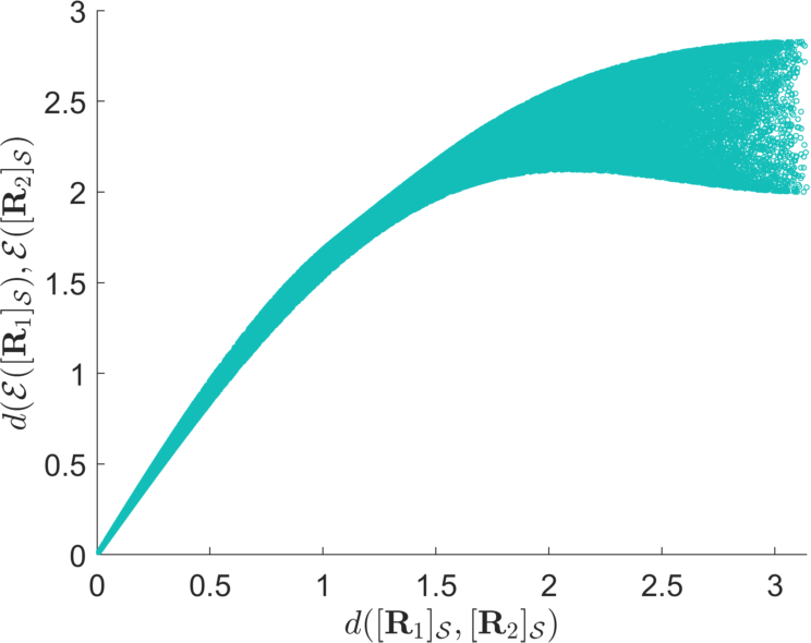
(a) Symmetry Group $C_{2}$

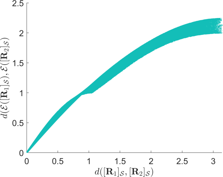
(b) Symmetry Group $C_{3}$

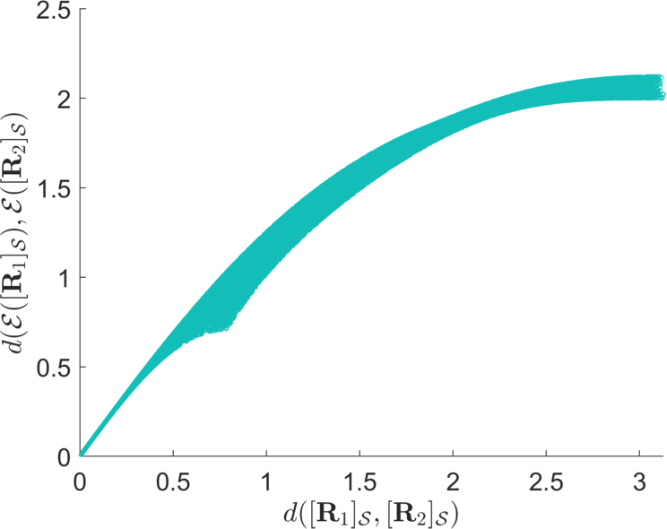
(c) Symmetry Group $C_{4}$

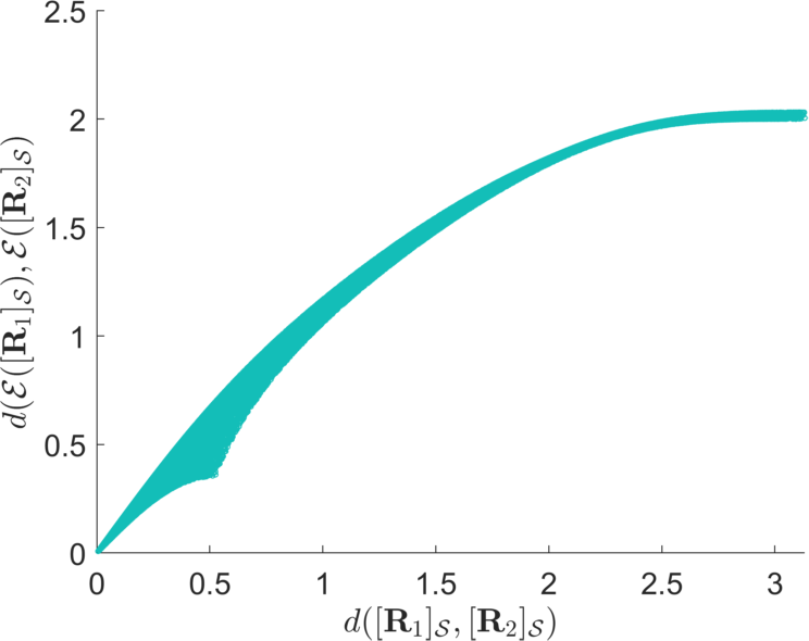
(d) Symmetry Group $C_{6}$

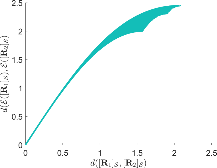
(e) Symmetry Group $D_{2}$

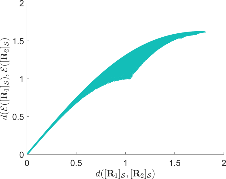
(f) Symmetry Group $D_{3}$

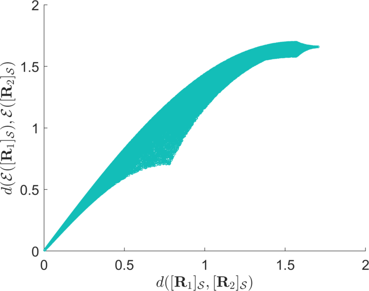
(g) Symmetry Group $D_{4}$

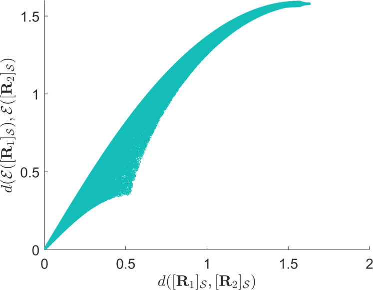
(h) Symmetry Group $D_{6}$

Fig. 1: Relation between the geodesic distance on the manifold and the Euclidean distance in the embedding for the embeddings reported in [2].

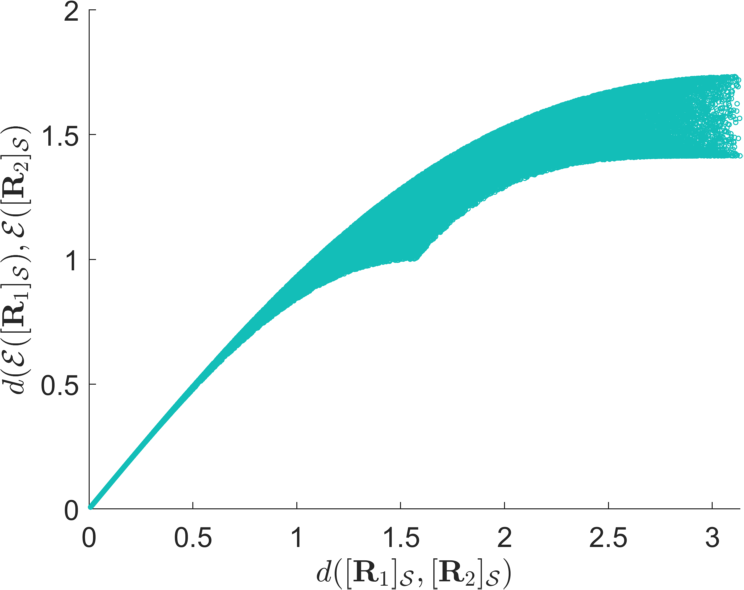
(a) Symmetry Group $C_{2}$

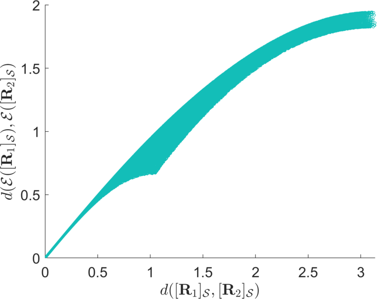
(b) Symmetry Group $C_{3}$

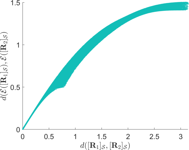
(c) Symmetry Group $C_{4}$

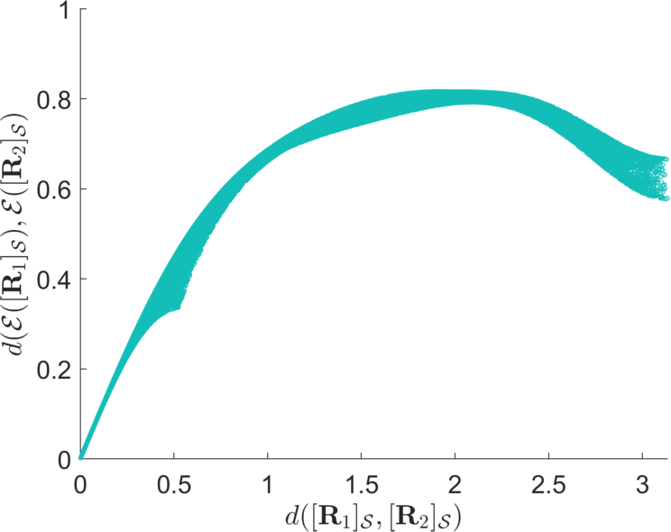
(d) Symmetry Group $C_{6}$

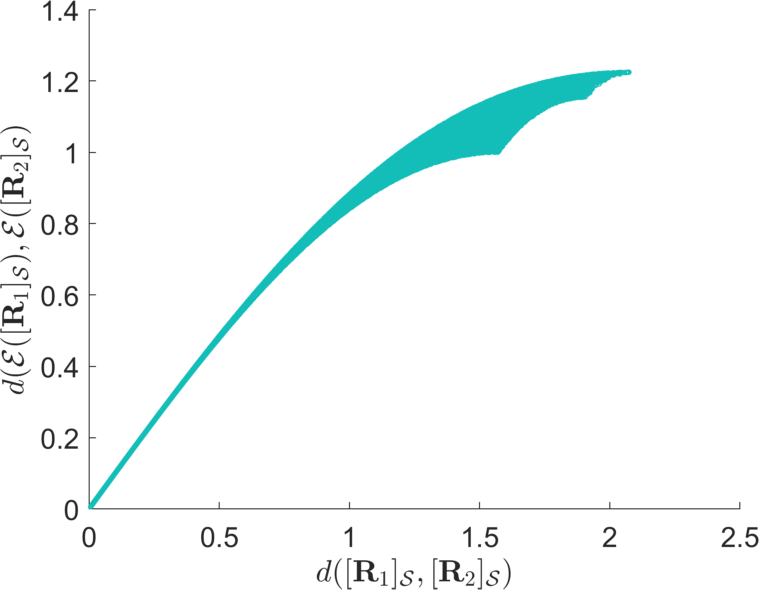
(e) Symmetry Group $D_{2}$

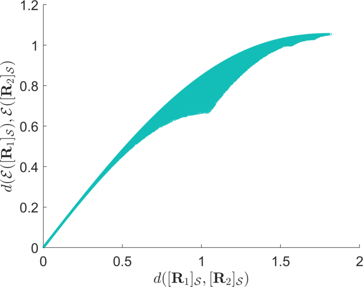
(f) Symmetry Group $D_{3}$

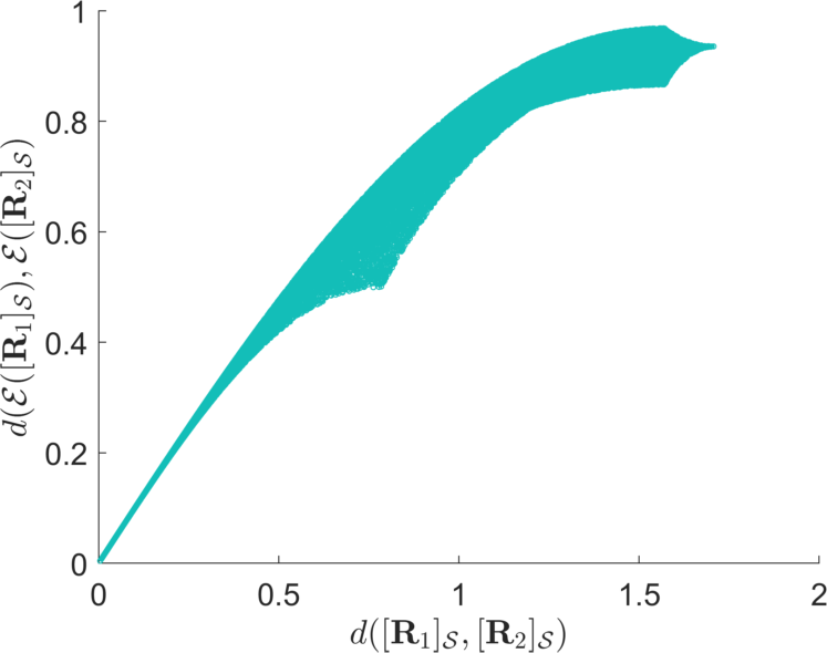
(g) Symmetry Group $D_{4}$

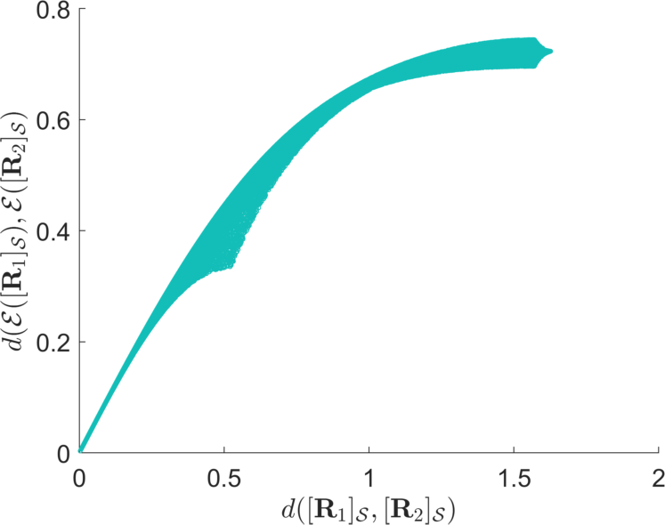
(h) Symmetry Group $D_{6}$

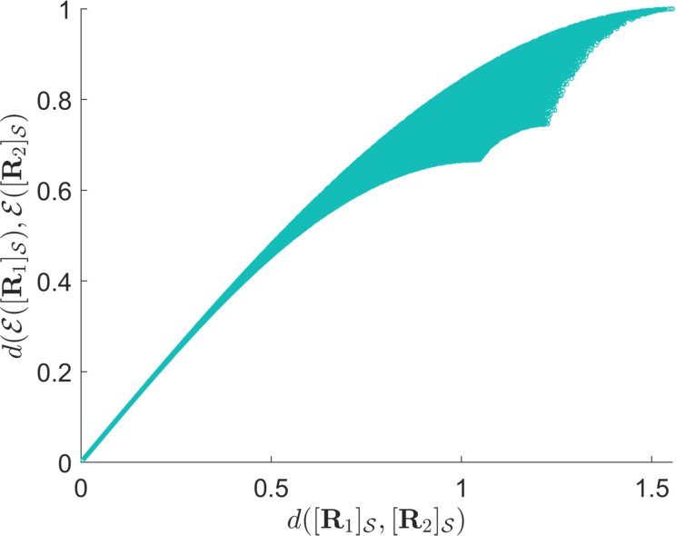
(i) Symmetry Group $T$

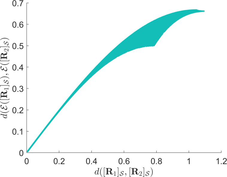
(j) Symmetry Group $O$

Fig. 2: Relation between the geodesic distance on the manifold and the Euclidean distance in the embedding for the locally isometric embeddings summarized in Table 2.

In Table 3 the upper and lower bounds $c_{\text{min}}$ and $c_{\text{max}}$ are listed for locally isometric embeddings from Table 2 . We would like to stress that non-locally-isometric embeddings might very well lead to better global bounds. Indeed, Table 4 provides alternative coefficients for the embeddings $\mathcal{E}_{\mathbf{\boldsymbol{u}},\mathcal{S}}^{\mathbf{\boldsymbol{\alpha}},\mathbf{\boldsymbol{\beta}}}$ which have better upper and lower bounds.

Table 3: The constants in equation (12) for all crystallographic symmetry groups $\mathcal{S}$

$\mathcal{S}$	$c_{\min}$	$c_{\max}$	$c_{\max}/c_{\min}$
$C_{2}$	$0.452$	$1$	$2.21$
$C_{3}$	$0.583$	$1$	$1.72$
$C_{4}$	$0.452$	$1$	$2.21$
$C_{6}$	$0.186$	$1$	$5.36$
$D_{2}$	$0.590$	$1$	$1.70$
$D_{3}$	$0.581$	$1$	$1.72$
$D_{4}$	$0.546$	$1$	$1.83$
$D_{6}$	$0.443$	$1$	$2.26$
$O$	$0.604$	$1$	$1.66$
$T$	$0.609$	$1$	$1.64$

Table 4: Factors for globally almost isometric embeddings for some symmetry groups $\mathcal{S}$

$\mathcal{S}$	$\mathbf{\boldsymbol{\beta}}$	$c_{\max}/c_{\min}$
$C_{2}$	$(1,0.5,0.5)$	$1.92$
$C_{3}$	$(1,0.67)$	$1.68$
$C_{4}$	$(1,0.6)$	$1.91$
$C_{6}$	$(1,0.93)$	$2.15$
$D_{3}$	$(1,1.03)$	$1.72$
$D_{4}$	$(1,1.11)$	$1.80$
$D_{6}$	$(1,1.65)$	$1.95$

Appendix A A binomial identity

For the calculation of $\left\lVert\smash{M_{\alpha}}\right\rVert$ in Lemma 2.8 we need the following nice Lemma for binomial coefficients.

Lemma A.1.

Let $\alpha\in 2\mathbb{N}$ be an even integer. Then we have the equality

$$\left(\alpha+1\right)\binom{\alpha}{\frac{\alpha}{2}}=\sum_{\begin{subarray}{c}i_{1},i_{2},i_{3}=0\\ i_{1}+i_{2}+i_{3}=\frac{\alpha}{2}\end{subarray}}^{\frac{\alpha}{2}}\binom{2i_{1}}{i_{1}}\binom{2i_{2}}{i_{2}}\binom{2i_{3}}{i_{3}}.$$

Proof.

With the general definition of the binomial coefficient $\binom{n}{k}=\frac{n(n-1)\cdots(n-(k-1))}{k!}$ for $k>0$ we obtain

$$\binom{2n}{n}=(-1)^{n}\cdot 4^{n}\cdot\binom{-\frac{1}{2}}{n}.$$

With this equation and the Chu-Vandermonde-identity it follows that

$$\sum_{\begin{subarray}{c}i_{1},i_{2},i_{3}=0\\ i_{1}+i_{2}+i_{3}=\frac{\alpha}{2}\end{subarray}}^{\frac{\alpha}{2}}\binom{2i_{1}}{i_{1}}\binom{2i_{2}}{i_{2}}\binom{2i_{3}}{i_{3}} =\sum_{\begin{subarray}{c}i_{1},i_{2},i_{3}=0\\ i_{1}+i_{2}+i_{3}=\frac{\alpha}{2}\end{subarray}}^{\frac{\alpha}{2}}\left(-1\right)^{i_{1}+i_{2}+i_{3}}\cdot 4^{i_{1}+i_{2}+i_{3}}\binom{-\frac{1}{2}}{i_{1}}\,\binom{-\frac{1}{2}}{i_{2}}\,\binom{-\frac{1}{2}}{i_{3}}$$

$$=\left(-1\right)^{\frac{\alpha}{2}}\cdot 4^{\frac{\alpha}{2}}\sum_{\begin{subarray}{c}i_{1},i_{2},i_{3}=0\\ i_{1}+i_{2}+i_{3}=\frac{\alpha}{2}\end{subarray}}^{\frac{\alpha}{2}}\binom{-\frac{1}{2}}{i_{1}}\,\binom{-\frac{1}{2}}{i_{2}}\,\binom{-\frac{1}{2}}{i_{3}}$$

$$=\left(-1\right)^{\frac{\alpha}{2}}\cdot 4^{\frac{\alpha}{2}}\binom{-\frac{3}{2}}{\frac{\alpha}{2}}$$

$$=\left(-1\right)^{\frac{\alpha}{2}}\cdot 4^{\frac{\alpha}{2}}\,\left(\frac{-\frac{3}{2}\left(-\frac{3}{2}-1\right)\cdots\left(-\frac{3}{2}-(\frac{\alpha}{2}-1)\right)}{\left(\frac{\alpha}{2}\right)!}\right)$$

$$=4^{\frac{\alpha}{2}}\,\left(\frac{\frac{3}{2}\left(\frac{3}{2}+1\right)\cdots\left(\frac{3}{2}+(\frac{\alpha}{2}-1)\right)}{\left(\frac{\alpha}{2}\right)!}\right)$$

$$=2^{\frac{\alpha}{2}}\,\left(\frac{3\cdot 5\cdot 7\cdots\left(\alpha+1\right)}{\left(\frac{\alpha}{2}\right)!}\right)$$

$$=\left(\alpha+1\right)\frac{2^{\frac{\alpha}{2}}\left(\frac{\alpha}{2}\right)!\cdot 3\cdot 5\cdot 7\cdots\left(\alpha-1\right)}{\left(\frac{\alpha}{2}\right)!^{2}}$$

$$=\left(\alpha+1\right)\binom{\alpha}{\frac{\alpha}{2}}.$$

∎

Appendix B Some trigonometrical sums

Here we calculate some trigonometric sums of the proofs in section 3. For the proof of Lemma 3.4 we need

$$\sum_{j_{1},j_{2}=0}^{k-1}\cos^{k-1}\tfrac{2\pi(j_{1}-j_{2})}{k}\sin\tfrac{2\pi j_{1}}{k}\cos\tfrac{2\pi j_{2}}{k} =\frac{1}{2}\sum_{j_{1},j_{2}=0}^{k-1}\cos^{k-1}\tfrac{2\pi(j_{1}-j_{2})}{k}\left(\sin\tfrac{2\pi(j_{1}-j_{2})}{k}+\sin\tfrac{2\pi(j_{1}+j_{2})}{k}\right)$$

$$=\frac{1}{2}\sum_{j_{1},j_{2}=0}^{k-1}\cos^{k-1}\tfrac{2\pi j_{1}}{k}\left(\sin\tfrac{2\pi j_{1}}{k}+\sin\tfrac{2\pi j_{2}}{k}\right)=0.$$ (13)

For the proof of Lemma 3.5 we need the following calculations. Using

$$\sum_{j=0}^{k-1}e^{\frac{2\pi ijn}{k}}=\begin{cases}k&n\in\mathbb{Z}\\ 0&else\end{cases}$$

we compute

$$\sum_{j=0}^{k-1}\cos^{k}\left(\frac{2\pi j}{k}\right) =\frac{1}{2^{k}}\sum_{j=0}^{k-1}\left(e^{\frac{2\pi ij}{k}}+e^{\frac{-2\pi ij}{k}}\right)^{k}=\frac{1}{2^{k}}\sum_{j=0}^{k-1}\sum_{\ell=0}^{k}\binom{k}{\ell}e^{\frac{4\pi ij\ell}{k}}$$

$$=\frac{1}{2^{k}}\sum_{\ell=0}^{k}\binom{k}{\ell}\sum_{j=0}^{k-1}e^{\frac{2\pi ij(2\,\ell)}{k}}=\begin{cases}\frac{k}{2^{k-1}}&\text{if }k\text{ odd}\\ \frac{1}{2^{k}}\left(\binom{k}{\frac{k}{2}}\cdot k+2k\right)&\text{if }k\text{ even}\end{cases},$$

$$\sum_{j=0}^{k-1}\cos^{k-2}\left(\frac{2\pi j}{k}\right) =\frac{1}{2^{k-2}}\sum_{j=0}^{k-1}\left(e^{\frac{2\pi ij}{k}}+e^{\frac{-2\pi ij}{k}}\right)^{k-2}=\frac{1}{2^{k-2}}\sum_{j=0}^{k-1}\sum_{\ell=0}^{k-2}\binom{k-2}{\ell}e^{\frac{2\pi ij(2\,\ell+2)}{k}}$$

$$=\frac{1}{2^{k-2}}\sum_{\ell=0}^{k-2}\binom{k}{\ell}\sum_{j=0}^{k-1}e^{\frac{2\pi ij(2\,\ell+2)}{k}}=\begin{cases}0&\text{if }k\text{ odd}\\ \frac{k}{2^{k-2}}\binom{k-2}{\frac{k}{2}-1}&\text{if }k\text{ even}\end{cases}.$$

We use this for the following calculations.

$$-\frac{(k-1)}{k}\sum_{j_{1}=0}^{k-1}\sum_{j_{2}=0}^{k-1}\cos^{k-2}\left(\frac{2\pi(j_{1}-j_{2})}{k}\right)\sin^{2}\left(\frac{2\pi(j_{1}-j_{2})}{k}\right)+\frac{1}{k}\sum_{j_{1}=0}^{k-1}\sum_{j_{2}=0}^{k-1}\cos^{k-1}\left(\frac{2\pi(j_{1}-j_{2})}{k}\right)\cos\left(\frac{2\pi(j_{1}-j_{2})}{k}\right)$$

$$\quad=-(k-1)\sum_{j=0}^{k-1}\cos^{k-2}\left(\frac{2\pi j}{k}\right)\sin^{2}\left(\frac{2\pi j}{k}\right)+\sum_{j=0}^{k-1}\cos^{k}\left(\frac{2\pi j}{k}\right)$$

$$\quad=-(k-1)\sum_{j=0}^{k-1}\cos^{k-2}\left(\frac{2\pi j}{k}\right)+k\,\sum_{j=0}^{k-1}\cos^{k}\left(\frac{2\pi j}{k}\right)$$

$$\quad=\begin{cases}\frac{k^{2}}{2^{k-1}}&\text{if }k\text{ odd}\\ -\frac{k(k-1)}{2^{k-2}}\binom{k-2}{\frac{k}{2}-1}+\frac{k^{2}}{2^{k}}\left(\binom{k}{\frac{k}{2}}+2\right)&\text{if }k\text{ even}\end{cases}.$$ (14)

Also for the proof of Lemma 3.5 we calculate the following.

$$\frac{1}{k}\sum_{j_{1}=0}^{k-1}\sum_{j_{2}=0}^{k-1}\cos^{k-1}\left(\frac{2\pi(j_{1}-j_{2})}{k}\right)\cos\left(\frac{2\pi j_{1}}{k}\right)\cos\left(\frac{2\pi j_{2}}{k}\right)$$

$$\quad=\frac{1}{k\,2^{k+1}}\sum_{j_{1}=0}^{k-1}\sum_{j_{2}=0}^{k-1}\left(e^{\frac{2\pi i(j_{1}-j_{2})}{k}}+e^{-\frac{2\pi i(j_{1}-j_{2})}{k}}\right)^{k-1}\left(e^{\frac{2\pi ij_{1}}{k}}+e^{-\frac{2\pi ij_{1}}{k}}\right)\left(e^{\frac{2\pi ij_{2}}{k}}+e^{-\frac{2\pi ij_{2}}{k}}\right)$$

$$\quad=\frac{1}{k\,2^{k+1}}\sum_{j_{1}=0}^{k-1}\sum_{j_{2}=0}^{k-1}\left(e^{\frac{2\pi i(j_{1}+j_{2})}{k}}+e^{-\frac{2\pi i(j_{1}+j_{2})}{k}}+e^{\frac{2\pi i(j_{1}-j_{2})}{k}}+e^{\frac{2\pi i(j_{2}-j_{1})}{k}}\right)\sum_{l=0}^{k-1}\binom{k-1}{l}e^{\frac{2\pi i(j_{1}-j_{2})(2l+1)}{k}}$$

$$\quad=\frac{1}{k\,2^{k+1}}\sum_{l=0}^{k-1}\binom{k-1}{l}\sum_{j_{1}=0}^{k-1}\sum_{j_{2}=0}^{k-1}\Big{(}e^{\frac{2\pi i((j_{1}-j_{2})(2l+1)+j_{1}+j_{2})}{k}}+e^{\frac{2\pi i((j_{1}-j_{2})(2l+1)-j_{1}-j_{2})}{k}}+e^{\frac{2\pi i(j_{1}-j_{2})(2l+2)}{k}}+e^{\frac{2\pi i(j_{1}-j_{2})(2l)}{k}}\Big{)}$$

$$\quad=\frac{1}{k\,2^{k+1}}\sum_{l=0}^{k-1}\binom{k-1}{l}\sum_{j_{1}=0}^{k-1}\sum_{j_{2}=0}^{k-1}\Big{(}e^{\frac{2\pi i(j_{1}(2l+2)-2lj_{2})}{k}}+e^{\frac{2\pi i(2lj_{1}-j_{2}(2l+2))}{k}}+e^{\frac{2\pi i(j_{1}-j_{2})(2l+2)}{k}}+e^{\frac{2\pi i(j_{1}-j_{2})(2l)}{k}}\Big{)}$$

$$\quad=\frac{k}{k\,2^{k+1}}\sum_{l=0}^{k-1}\binom{k-1}{l}\sum_{j=0}^{k-1}e^{\frac{2\pi ij(2l+2)}{k}}+e^{\frac{2\pi ij(2l)}{k}}$$

$$\quad=\begin{cases}\frac{k}{2^{k}}&\text{if }k\text{ is odd}\\ \frac{k}{2^{k+1}}\left(2+\binom{k-1}{\frac{k}{2}}+\binom{k-1}{\frac{k}{2}-1}\right)&\text{if }k\text{ is even}\end{cases}.$$ (15)

References

- Adams et al. [1993] B. L. Adams, S. I. Wright, K. Kunze, Orientation imaging: The emergence of a new microscopy, Metall Mater Trans A 24 (1993) 819–831.
- Arnold et al. [2018] R. Arnold, P. Jupp, H. Schaeben, Statistics of ambiguous rotations, J. Mult. Anal. 165 (2018) 73–85.
- Bajaj et al. [2013] C. Bajaj, B. Bauer, R. Bettadapura, A. Vollrath, Nonuniform Fourier transforms for rigid-body and multidimensional rotational correlations, SIAM J. Sci. Comput. 35 (2013) B821–B845.
- Bunge [1982] H. J. Bunge, Texture Analysis in Material Science, Butterworths, 1982.
- Coifman and Lafon [2006] R. R. Coifman, S. Lafon, Diffusion maps, Appl. Comput. Harmon. Anal. 21 (2006) 5 – 30. Special Issue: Diffusion Maps and Wavelets.
- Comon et al. [2008] P. Comon, G. Golub, L. Lim, B. Mourrain, Symmetric Tensors and Symmetric Tensor Rank, SIAM J. Matrix Anal. Appl. 30 (2008) 1254–1279.
- Cremers and Strekalovskiy [2013] D. Cremers, E. Strekalovskiy, Total cyclic variation and generalizations, J. Math. Imaging Vision 47 (2013) 258–277.
- Engler et al. [1994] O. Engler, G. Gottstein, J. Pospiech, J. Jura, Statistics, evaluation and representation of single grain orientation measurements, Mater. Sci. Forum 157 –- 162 (1994) 259–274.
- Gawlik and Leok [2018] E. S. Gawlik, M. Leok, Embedding-based interpolation on the special orthogonal group, SIAM J. Scientific Computing 40 (2018) A721–A746.
- Grohs et al. [2017] P. Grohs, M. Sprecher, T. Yu, Scattered manifold-valued data approximation, Numer. Math. 135 (2017) 987–1010.
- Hendriks [1990] H. Hendriks, Nonparametric estimation of a probability density on a Riemannian manifold using Fourier expansion, Ann. Statist. 18 (1990) 832–849.
- Hielscher [2013] R. Hielscher, Kernel density estimation on the rotation group and its application to crystallographic texture analysis, J. Multivariate Anal. 119 (2013) 119–143.
- Horn [1987] B. Horn, Closed-form solution of absolute orientation using unit quaternions, J. Opt. Soc. Am 4 (1987) 629–642.
- Jupp [2005] P. E. Jupp, Sobolev tests of goodness of fit of distributions on compact riemannian manifolds, Ann. Statist. 33 (2005) 2957–2966.
- Kim [1998] P. T. Kim, Deconvolution density estimation on SO(N), Ann. Statist. 26 (1998) 1083–1102.
- Krakow et al. [2017] R. Krakow, R. J. Bennett, D. N. Johnstone, Z. Vukmanovic, W. Solano-Alvarez, S. J. Laine, J. F. Einsle, P. A. Midgley, C. M. F. Rae, R. Hielscher, On three-dimensional misorientation spaces, Proc. R. Soc. A 473 (2017).
- Lee [2012] J. Lee, Introduction to Smooth Manifolds, Springer-Verlag New York, second edition, 2012.
- Nash [1954] J. Nash, C1 isometric imbeddings, Annals of Mathematics 60 (1954) 383–396.
- Pelletier [2005] B. Pelletier, Kernel density estimation on Riemannian manifolds, Statist. Probab. Lett. 73 (2005) 297–304.
- Rahman et al. [2005] I. Rahman, I. Drori, V. Stodden, D. Donoho, P. Schröder, Multiscale representations for manifold-valued data, Multiscale Model. Sim. 4 (2005) 1201–1232.
- Rosman et al. [2012] G. Rosman, M. M. Bronstein, A. M. Bronstein, A. Wolf, R. Kimmel, Group-valued regularization framework for motion segmentation of dynamic non-rigid shapes, in: A. M. Bruckstein, B. M. ter Haar Romeny, A. M. Bronstein, M. M. Bronstein (Eds.), Scale Space and Variational Methods in Computer Vision, Springer Berlin Heidelberg, Berlin, Heidelberg, 2012, pp. 725–736.
- Rosman et al. [2014] G. Rosman, X.-C. Tai, R. Kimmel, A. Bruckstein, Augmented-Lagrangian regularization of matrix-valued maps, Methods Appl. Anal. 21 (2014) 121–138.
- Udrişte [1994] C. Udrişte, Convex functions and optimization methods on Riemannian manifolds, volume 297 of Mathematics and its Applications, Kluwer Academic Publishers Group, Dordrecht, 1994.
- Verma [2013] N. Verma, Distance preserving embeddings for general n-dimensional manifolds, J. Mach. Learn. Res. 14 (2013) 2415–2448.
- Xie and Yu [2007] G. Xie, T. P.-Y. Yu, Smoothness equivalence properties of manifold-valued data subdivision schemes based on the projection approach, SIAM J. Numer. Anal. 45 (2007) 1200–1225.
- Zefran et al. [1998] M. Zefran, V. Kumar, C. B. Croke, On the generatation of smooth three-dimensional rigid body motions, IEEE Trans. Robot. Autom. 14 (1998) 576–589.