Generalized noncommutative Snyder spaces and projective geometry

Abstract:

Given a group of kinematical symmetry generators, one can construct a compatible noncommutative spacetime and deformed phase space by means of projective geometry. This was the main idea behind the very first model of noncommutative spacetime, proposed by H.S. Snyder in 1947. In this framework, spacetime coordinates are the translation generators over a manifold that is symmetric under the required generators, while momenta are projective coordinates on such a manifold. In these proceedings we review the construction of Euclidean and Lorentzian noncommutative Snyder spaces and investigate the freedom left by this construction in the choice of the physical momenta, because of different available choices of projective coordinates. In particular, we derive a quasi-canonical structure for both the Euclidean and Lorentzian Snyder noncommutative models such that their phase space algebra is diagonal although no longer quadratic.

1 Introduction

Noncommutative spacetimes play an important role in quantum gravity research, since they provide a way to formalize the “foamy” or fuzzy features that spacetime is thought to acquire at the Planck scale [1, 2, 3]. Somewhat related to this, another possibility that has been long entertained in quantum gravity research is that of the emergence of a minimal length uncertainty and the associated generalised uncertainty principle (GUP) [2, 4, 5, 6, 7].

It is interesting to investigate whether such quantum features can be introduced without spoiling invariance under relativistic symmetries and how they are related to each other. This was the driving idea of H.S. Snyder’s work [8] in 1947: he was able to show that one can construct a noncommutative spacetime (and correspondingly deformed phase space leading to a GUP [7, 9, 10]) that is invariant under the usual special-relativistic Lorentz symmetries. The construction assumes that momentum space is a de Sitter manifold, spacetime coordinates are identified with the translation generators on this manifold (so that their noncommutativity is a consequence of the manifold’s curvature), and physical momenta are taken to be the Beltrami projective coordinates on the manifold. Physical momenta thus constructed satisfy two requirements: they are commutative and transform classically under Lorentz symmetries.

In recent work [11] we extended the construction to noncommutative spacetimes that are compatible with Galilean and Carrollian relativistic symmetries. There, we noticed that there is some freedom in the choice of the physical momenta, since different projective coordinates on the momentum manifold satisfy the two requirements mentioned above. This freedom is very relevant for the study of the phenomenological consequences of the Snyder model [10, 12, 13, 14, 15, 16, 17, 18, 19], since different choices of momenta and resulting different phase spaces would lead to different physical predictions.

In these proceedings we investigate in depth the issue of the freedom in the choice of momenta, focussing on Snyder models with Euclidean and Lorentzian symmetries. We expose different deformed phase spaces that arise from different choices of physical momenta. We find that any choice of projective coordinates on the curved manifold gives a viable choice of momenta. Moreover, we derive a quasi-canonical structure for both the Euclidean and Lorentzian Snyder noncommutative models such that their phase space algebra is diagonal although no longer quadratic. We show that the momenta associated to this choice can be identified with the ambient coordinates of the curved manifold.

2 Projective geometry construction of the Snyder–Euclidean model

We start by reviewing the construction of the two-dimensional (2D) Snyder–Euclidean noncommutative space, emphasizing the different possible choices of spatial momenta and their implications.

Since we require that the Snyder–Euclidean noncommutative space is invariant under rotations, we take spatial coordinates to be the translation generators over a 2D manifold with constant Gaussian curvature $\omega$ that is either a sphere ($\omega>0$) or a two-sheeted hyperboloid ($\omega<0$), and enjoys ${\rm SO}(3)$ or ${\rm SO}(2,1)$ symmetry, respectively. Specifically, the Lie algebra of isometries of the manifold is generated by the rotation $J$ and translations $P_{1},P_{2}$, with commutation relations

$$[J,P_{1}]=P_{2},\qquad[J,P_{2}]=-P_{1},\qquad[P_{1},P_{2}]=\omega\,J.$$ (1)

As we showed in [11], the homogeneous spaces of the Lie groups with Lie algebras (1) (i.e. the curved manifolds) can be described in terms of embedding coordinates $(s_{3},s_{1},s_{2})$ that satisfy the following constraint

$$\Sigma_{\omega}\ :\ s_{3}^{2}+\omega\left(s_{1}^{2}+s_{2}^{2}\right)=1.$$ (2)

In terms of these ambient coordinates, the vector fields corresponding to the symmetry transformations read

$$P_{1}=s_{3}\,\frac{\partial}{\partial s_{1}}-\omega\,s_{1}\,\frac{\partial}{\partial s_{3}},\qquad P_{2}=s_{3}\,\frac{\partial}{\partial s_{2}}-\omega\,s_{2}\,\frac{\partial}{\partial s_{3}},\qquad J=s_{2}\,\frac{\partial}{\partial s_{1}}-s_{1}\,\frac{\partial}{\partial s_{2}}.$$ (3)

The Snyder–Euclidean noncommutative space is then obtained upon the identification

$$x_{1}:=P_{1},\qquad x_{2}:=P_{2},$$ (4)

so that spatial coordinates inherit the noncommutativity from the curvature of the underlying manifold:

$$\left[x_{1},x_{2}\right]=\omega\,J.$$ (5)

In order to construct a full phase space we define momenta as objects that are commutative and transform as vector under rotations. It turns out that several kinds of projective coordinates of the curved manifold satisfy these requirements [11]. The ones corresponding to the original choice by Snyder [8] are the Beltrami projective coordinates:

$$p_{1}:=\frac{s_{1}}{s_{3}},\qquad p_{2}:=\frac{s_{2}}{s_{3}}.$$ (6)

The coordinates $(p_{1},p_{2})$ are obtained as the central stereographic projection with pole $(0,0,0)\in\mathbb{R}^{3}$ of a point $Q=(s_{3},s_{1},s_{2})\in\Sigma_{\omega}$ (2) onto the projective plane with $s_{3}=1$ as depicted in figure 1. This establishes the relations $(i=1,2)$

$$s_{3}=\frac{1}{\sqrt{1+\omega(p_{1}^{2}+p_{2}^{2})}},\qquad s_{i}=\frac{p_{i}}{\sqrt{1+\omega(p_{1}^{2}+p_{2}^{2})}},\qquad p_{i}=\frac{s_{i}}{s_{3}}.$$ (7)

Figure 1: Beltrami projective coordinates for the sphere on the left and the hyperboloid on the right.

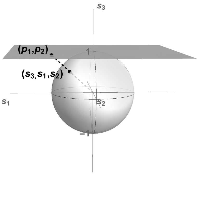
Thus the origin $O=(1,0,0)\in\Sigma_{\omega}$ projects to the origin $(p_{1},p_{2})=(0,0)$ in the projective space. The domain of $(p_{1},p_{2})$ depends on the sign of the curvature $\omega$ since the equations (7) require that

$$1+\omega(p_{1}^{2}+p_{2}^{2})>0.$$ (8)

In particular we find that [20]:

• When the underlying curved manifold is a sphere, corresponding to the Snyder–Euclidean model with $\omega>0$, the condition (8) is always satisfied, so that there is no restriction on the momentum domain

  $$p_{i}\in(-\infty,+\infty).$$ (9)

  This corresponds to the fact that the projection sends the points in the equator in $\Sigma_{\omega}$ (2), characterized by $s_{3}=0$ and $s_{1}^{2}+s_{2}^{2}=1/\omega$, to infinity in the projective plane, so that the projection (7) is well-defined for the whole hemisphere with $s_{3}>0$.

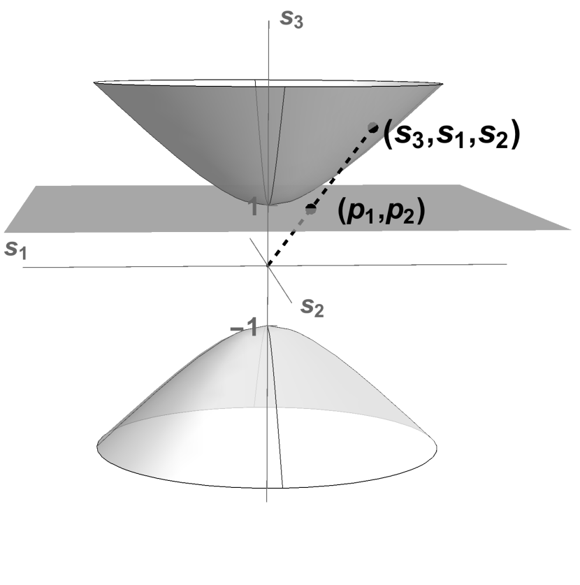
• When the underlying curved manifold is a hyperbolic space (the sheet of the hyperboloid with $s_{3}\geq 1$), corresponding to the Snyder–Euclidean model with $\omega<0$, the momentum space domain is restricted, since the condition (8) is only satisfied for

  $$p_{1}^{2}+p_{2}^{2}<\frac{1}{|\omega|}.$$ (10)

  Hence the momentum space can be identified with the interior of a Klein disk with radius $1/\sqrt{|\omega|}$. In fact, the projection (7) sends the points at the infinity in the upper sheet of the hyperboloid with $s_{3}\to\infty$ to the circle $p_{1}^{2}+p_{2}^{2}=\frac{1}{|\omega|}$ (that is, the boundary of the Klein disk).

With the choice of the physical momenta (6) one obtains the following phase space [11]:

$$\begin{array}[]{ll}\left[x_{1},x_{2}\right]=\omega\,J,&\qquad\left[p_{1},p_{2}\right]=0,\\[4.0pt] \left[x_{1},p_{1}\right]=1+\omega\,p_{1}^{2},&\qquad\left[x_{1},p_{2}\right]=\omega\,p_{1}p_{2},\\[4.0pt] \left[x_{2},p_{2}\right]=1+\omega\,p_{2}^{2},&\qquad\left[x_{2},p_{1}\right]=\omega\,p_{1}p_{2},\end{array}$$ (11)

where the rotation generator $J$ becomes the angular momentum in (11) given by

$$J=x_{1}\,p_{2}-x_{2}\,p_{1}.$$ (12)

One can verify by direct computation that these phase space variables satisfy the Jacobi identities. Moreover, both the space coordinates $x_{i}$ and momenta $p_{i}$ are transformed as vectors under $J$:

$$[J,x_{1}]=x_{2},\qquad[J,x_{2}]=-x_{1},\qquad[J,p_{1}]=p_{2},\qquad[J,p_{2}]=-p_{1},$$ (13)

so that the phase space (11) is invariant under rotations, as required.

2.1 Different choices of momenta in the Snyder–Euclidean model

As already noticed in [8], the choice of physical momenta is not univocally determined by the requirements of being commutative and transforming as vectors under rotations. In fact, these requirements by themselves do not completely fix the functional dependence of momenta on the embedding coordinates $(s_{3},s_{1},s_{2})$. In particular, the Beltrami projective coordinates are not the only available option. For example, one could identify momenta with the Poincaré projective coordinates $(\tilde{p}_{1},\tilde{p}_{2})$, which come from the stereographic projection with pole $(-1,0,0)\in\mathbb{R}^{3}$ onto the projective plane with $s_{3}=0$ as shown in figure 2. In this case the relation between the ambient and the projective coordinates reads $(i=1,2)$

$$s_{3}=\frac{1-\omega(\tilde{p}_{1}^{2}+\tilde{p}_{2}^{2})}{{1+\omega(\tilde{p}_{1}^{2}+\tilde{p}_{2}^{2})}},\qquad s_{i}=\frac{2{\tilde{p}_{i}}}{{1+\omega(\tilde{p}_{1}^{2}+\tilde{p}_{2}^{2})}},\qquad{\tilde{p}_{i}}=\frac{s_{i}}{1+s_{3}}.$$ (14)

Figure 2: Poincaré projective coordinates for the sphere on the left and the hyperboloid on the right.

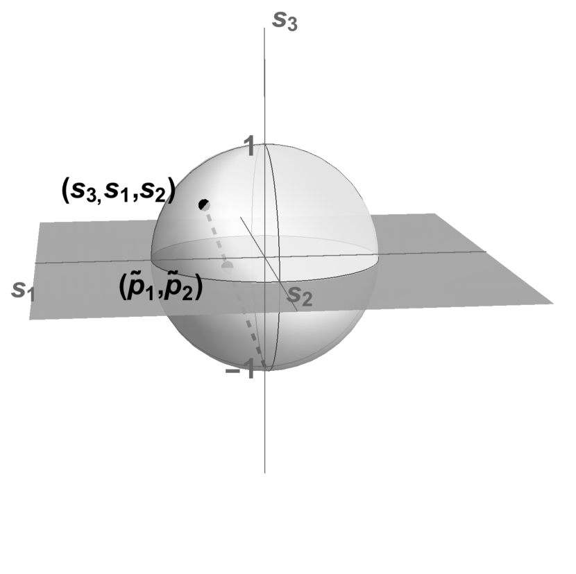
This projection is well-defined for any point $Q=(s_{3},s_{1},s_{2})\in\Sigma_{\omega}$ (2) except for the pole $(-1,0,0)$ which projects to the infinity in both the sphere and in the hyperbolic space. The origin $O=(1,0,0)\in\Sigma_{\omega}$ again projects to the origin $(\tilde{p}_{1},\tilde{p}_{2})=(0,0)$ in the projective space. In order to deduce the domain of the Poincaré coordinates $(\tilde{p}_{1},\tilde{p}_{2})$ we shall make use of the following expression coming from (14):

$$\tilde{p}_{1}^{2}+\tilde{p}_{2}^{2}=\frac{1}{\omega}\,\frac{1-s_{3}}{1+s_{3}}.$$ (15)

Thus we find that [20]:

• On the sphere with $\omega>0$, it is verified that $-1<s_{3}\leq 1$ so that the relation (15) gives

  $$\tilde{p}_{i}\in(-\infty,+\infty).$$ (16)

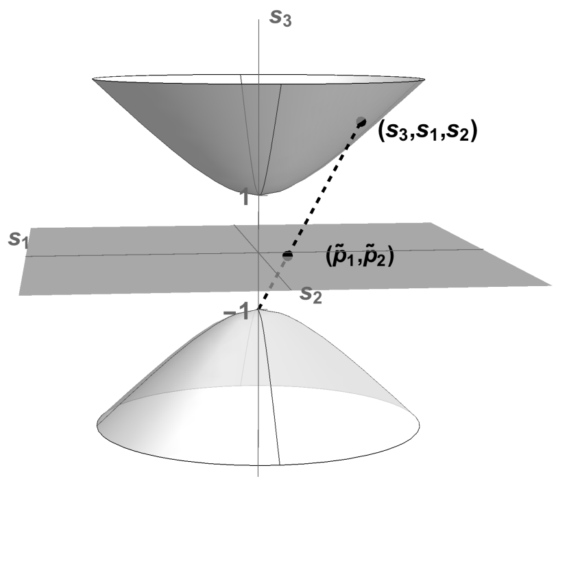
• On the hyperbolic case with $\omega<0$ and $s_{3}\geq 1$, the condition (15) leads to a restriction of the domain

  $$\tilde{p}_{1}^{2}+\tilde{p}_{2}^{2}=\frac{1}{|\omega|}\,\frac{s_{3}-1}{s_{3}+1}<\frac{1}{|\omega|},$$ (17)

  which can be identified with the interior of a Poincaré disk (or conformal disk model) with radius $1/\sqrt{|\omega|}$, whose boundary corresponds to the points with $s_{3}\to\infty$.

Taking the Poincaré coordinates as physical momenta and identifying space coordinates with the translations over the curved manifold as done before, one obtains a new Snyder–Euclidean phase space given by

$$\begin{array}[]{ll}\left[x_{1},x_{2}\right]=\omega\,J,&\qquad\left[\tilde{p}_{1},\tilde{p}_{2}\right]=0,\\[4.0pt] \left[x_{1},\tilde{p}_{1}\right]=\frac{1}{2}\bigl{(}1+\omega(\tilde{p}_{1}^{2}-\tilde{p}_{2}^{2})\bigr{)},&\qquad\left[x_{1},\tilde{p}_{2}\right]=\omega\,\tilde{p}_{1}\tilde{p}_{2},\\[4.0pt] \left[x_{2},\tilde{p}_{2}\right]=\frac{1}{2}\bigl{(}1+\omega(\tilde{p}_{2}^{2}-\tilde{p}_{1}^{2})\bigr{)},&\qquad\left[x_{2},\tilde{p}_{1}\right]=\omega\,\tilde{p}_{1}\tilde{p}_{2},\end{array}$$ (18)

where the angular momentum $J$ is now represented by

$$J=2\,\frac{x_{1}\tilde{p}_{2}-x_{2}\tilde{p}_{1}}{1-\omega(\tilde{p}_{1}^{2}+\tilde{p}_{2}^{2})}.$$ (19)

Notice that the above expression is consistently written since

$$\bigl{[}x_{1}\tilde{p}_{2}-x_{2}\tilde{p}_{1},\tilde{p}_{1}^{2}+\tilde{p}_{2}^{2}\bigr{]}=0.$$ (20)

The phase space (18) is viable in the sense that its variables satisfy the Jacobi identities and the invariance under rotations is retained, that is, momenta $\tilde{p}_{i}$ transform as vectors under $J$ in the same form given in (13).

Thus the expressions (18) provide another way to define 2D Snyder–Euclidean models. Moreover, the two models (11) and (18) are related by the following non-linear change of momenta $(i=1,2)$:

$$\tilde{p}_{i}=\frac{p_{i}}{1+\sqrt{1+\omega(p_{1}^{2}+p_{2}^{2})}},\qquad p_{i}=\frac{2\tilde{p}_{i}}{1-{\omega(\tilde{p}_{1}^{2}+\tilde{p}_{2}^{2})}}.$$ (21)

Recall that momenta commute and notice also that the above map does not involve the space coordinates, so preserving the noncommutative Snyder space $[x_{1},x_{2}]=\omega\,J$, as it should be, although the explicit representation for the angular momentum $J$ changes.

We remark that other types of projections (choosing another pole and plane $s_{3}=$ constant) would lead to different explicit forms for the 2D Snyder–Euclidean models, keeping the space coordinates but with different momenta. These possibilities would be related among themselves through transformations of the momenta similarly to (21).

2.2 Quasi-canonical structure of the Snyder–Euclidean model

By taking into account the above results, it is rather natural to analyse whether the structure of the quadratic algebra (11) can further be simplified. And actually it is possible to choose momenta in such a manner that the phase space algebra becomes diagonal. Indeed, if we apply the change of momenta given by

$$\pi_{i}=\frac{p_{i}}{\sqrt{1+\omega(p_{1}^{2}+p_{2}^{2})}},\qquad p_{i}=\frac{\pi_{i}}{\sqrt{1-\omega(\pi_{1}^{2}+\pi_{2}^{2})}},$$ (22)

the commutators (11) reduce to

$$\begin{array}[]{l}[x_{1},x_{2}]=\omega\,J,\qquad[\pi_{1},\pi_{2}]=0,\\[4.0pt] [x_{i},\pi_{j}]=\delta_{ij}\sqrt{1-\omega(\pi_{1}^{2}+\pi_{2}^{2})}\,.\end{array}$$ (23)

As a consequence, the algebra (23) is no longer quadratic but conveys commutativity of the non-diagonal terms, $[x_{1},\pi_{2}]=[x_{2},\pi_{1}]=0$. This diagonal algebra was originally considered in [21] and then linked to the Snyder model in [22, 19].

Furthermore, the diagonal brackets are deformed in terms of the curvature parameter $\omega$ in a symmetrical manner governed by $\pi_{1}^{2}+\pi_{2}^{2}$. The power series expansion in terms of $\omega$ turns out to be

$$[x_{1},\pi_{1}]=[x_{2},\pi_{2}]=\sqrt{1-\omega(\pi_{1}^{2}+\pi_{2}^{2})}=\left(1-\frac{1}{2}\omega(\pi_{1}^{2}+\pi_{2}^{2})\right)+o[\omega^{2}],$$ (24)

hence for a small value of $\omega$, the Snyder–Euclidean phase space (23) can be taken as a quadratic algebra.

The angular momentum $J$ adopts the non-standard representation

$$J=\frac{x_{1}\,\pi_{2}-x_{2}\,\pi_{1}}{\sqrt{1-\omega(\pi_{1}^{2}+\pi_{2}^{2})}},$$ (25)

as in Poincaré variables (19), where we note that

$$\bigl{[}x_{1}\,\pi_{2}-x_{2}\,\pi_{1},\pi_{1}^{2}+\pi_{2}^{2}\bigr{]}=0.$$ (26)

Still, the new momenta defined in (22) satisfy the required properties: they are commutative and transform as vectors under rotations. This can easily be checked by explicitly verifying that the same commutators as in (13) hold for the new momenta $(\pi_{1},\pi_{2})$ and $J$.

The domain for the new momenta $(\pi_{1},\pi_{2})$ is of course different from that of $(p_{1},p_{2})$, but it is so in a consistent way, since the map (22) implies the identity

$$1+\omega(p_{1}^{2}+p_{2}^{2})=\frac{1}{1-\omega(\pi_{1}^{2}+\pi_{2}^{2})},$$ (27)

thus leading to the constraint (see (8))

$$1+\omega(p_{1}^{2}+p_{2}^{2})>0\quad\Longleftrightarrow\quad 1-\omega(\pi_{1}^{2}+\pi_{2}^{2})>0.$$ (28)

Therefore the domain of the new momentum space is interchanged between the spherical and hyperbolic cases, that is

$$\begin{array}[]{ll}\mbox{Snyder--Euclidean space with $\omega>0$:}&\pi_{1},\pi_{2}\in\bigl{(}-1/\sqrt{|\omega|},+1/\sqrt{|\omega|}\,\bigr{)}.\\[2.0pt] \mbox{Snyder--Euclidean space with $\omega<0$:}&\pi_{1},\pi_{2}\in(-\infty,+\infty).\end{array}$$ (29)

Since we have previously seen that the momenta $p_{i}$ and $\tilde{p}_{i}$ have a geometrical interpretation as projective coordinates on the curved momentum manifold, it is natural to wonder about the geometrical role of this alternative choice $\pi_{i}$. By comparison between the maps (7) and (22) it is immediate to see that the momenta $\pi_{i}$ have a direct relation with the momentum space ambient coordinates $s_{i}$:

$$s_{1}\equiv\pi_{1},\qquad s_{2}\equiv\pi_{2},\qquad s_{3}\equiv\sqrt{1-\omega(\pi_{1}^{2}+\pi_{2}^{2})}.$$ (30)

From this viewpoint the ambient coordinates $(s_{1},s_{2})$ are just the momenta $(\pi_{1},\pi_{2})$, while the third coordinate $s_{3}$ determines the geodesic distance, say $p_{r}$, between the origin $O=(1,0,0)$ and a point $Q=(s_{3},s_{1},s_{2})\in\Sigma_{\omega}$ (2) in the 3D ambient space (see [20, 23]), namely

$$s_{3}=\cos(\sqrt{\omega}\,p_{r}).$$ (31)

This is just the term deforming the canonical commutators $[x_{i},\pi_{i}]$.

It is worth remarking that the generalization of all the results presented in this section to arbitrary dimension $N$, so with ${\rm SO}(N+1)$ and ${\rm SO}(N,1)$ symmetry, is straightforward. In fact, the necessary tools, such as the $(N+1)$ ambient coordinates along with the $N$ Beltrami and Poincaré coordinates on the $N$D spherical and hyperbolic spaces in terms of their constant (sectional) curvature, can be found in [24].

3 Projective geometry construction of the Snyder–Lorentzian model

Similar issues as the ones exposed for the Snyder–Euclidean model also emerge in the kinematical cases covering Snyder–Lorentzian, Snyder–Galilean and Snyder–Carrollian models which were developed in [11]. In these notes we focus on the Snyder–Lorentzian model, since the corresponding momentum choices for the Galilean and Carrollian cases can be deduced by following the limiting procedures described in [11].

Invariance under Lorentzian symmetries is achieved by taking the (3+1)D spacetime coordinates to be the translations over a (3+1)D manifold with constant sectional curvature equal to $-\Lambda$, where $\Lambda$ is the cosmological constant. This is either de Sitter ($\Lambda>0$) or Anti-de Sitter ($\Lambda<0$) manifold, enjoying ${\rm SO}(4,1)$ and ${\rm SO}(3,2)$ symmetry, respectively. The algebra of isometries is generated by Lorentzian boosts $K_{i}$, rotations $J_{i}$ and spacetime translations $P_{\alpha}$ which fulfil the following commutation rules

$$\begin{array}[]{lll}[J_{i},J_{j}]=\epsilon_{ijk}J_{k},&\qquad[J_{i},P_{j}]=\epsilon_{ijk}P_{k},&\qquad[J_{i},K_{j}]=\epsilon_{ijk}K_{k},\\[4.0pt] \displaystyle{[K_{i},P_{0}]=P_{i}},&\qquad{[K_{i},P_{j}]=\frac{1}{c^{2}}\,\delta_{ij}P_{0}},&\qquad{[K_{i},K_{j}]=-\frac{1}{c^{2}}\,\epsilon_{ijk}J_{k}},\\[4.0pt] [P_{0},P_{i}]=-\Lambda\,K_{i},&\qquad[P_{i},P_{j}]=\Lambda\,\frac{1}{c^{2}}\,\epsilon_{ijk}J_{k},&\qquad[P_{0},J_{i}]=0,\end{array}$$ (32)

where $c$ is the speed of light; hereafter Latin indices run as $i,j,k=1,2,3$, Greek indices run as $\alpha=0,1,2,3$ and sum over repeated indices will be understood.

As we showed in [11], a homogeneous space of the Lie group with Lie algebra (32), corresponding to the momentum space in the Snyder model, can be described in terms of embedding coordinates $(s_{4},s_{0},s_{1},s_{2},s_{3})$ in a 5D ambient manifold that satisfy the constraint

$$\Sigma_{\Lambda}\,:\ s_{4}^{2}-\Lambda\,s_{0}^{2}+\frac{\Lambda}{c^{2}}\bigl{(}s_{1}^{2}+s_{2}^{2}+s_{3}^{2}\bigr{)}=1.$$ (33)

In terms of these coordinates, the isometries generators on the curved manifolds read

$$P_{0}=s_{4}\,\frac{\partial}{\partial s_{0}}+\Lambda\,s_{0}\,\frac{\partial}{\partial s_{4}}\,,\qquad\ \,P_{i}=-s_{4}\,\frac{\partial}{\partial s_{i}}+\frac{\Lambda}{c^{2}}\,s_{i}\,\frac{\partial}{\partial s_{4}}\,,$$

$$K_{i}=s_{0}\,\frac{\partial}{\partial s_{i}}+\frac{1}{c^{2}}\,s_{i}\,\frac{\partial}{\partial s_{0}}\,,\qquad J_{i}=-\epsilon_{ijk}\,s_{j}\,\frac{\partial}{\partial s_{k}}\,.$$ (34)

The Snyder–Lorentzian noncommutative spacetime is then obtained upon the identification

$$x^{0}:=\frac{1}{c}\,P_{0},\qquad x^{i}:=-c\,P_{i},$$ (35)

yielding

$$\left[x^{0},x^{i}\right]=\Lambda\,K_{i},\qquad\left[x^{i},x^{j}\right]=\Lambda\,\epsilon_{ijk}J_{k},$$ (36)

so that spacetime coordinates inherit the noncommutativity from the curvature of the (Anti)-de Sitter manifold.

The full Snyder–Lorentzian phase space is constructed by introducing momenta as objects that are commutative and transform as vectors under Lorentz transformations. As seen for the Snyder–Euclidean model, the choice is not univocal. In the case of Beltrami projective coordinates $(q_{0},q_{1},q_{2},q_{3})$, these come from the central stereographic projection in the 5D ambient space with pole $(0,0,0,0,0)$ of a point $Q=(s_{4},s_{0},s_{1},s_{2},s_{3})\in\Sigma_{\Lambda}$ (33) onto the projective hyperplane with $s_{4}=1$, namely

$$s_{4}=\frac{1}{\sqrt{1-\Lambda\,q_{0}^{2}+\frac{\Lambda}{c^{2}}(q_{1}^{2}+q_{2}^{2}+q_{3}^{2})}},\quad\ s_{\alpha}=\frac{q_{\alpha}}{\sqrt{1-\Lambda\,q_{0}^{2}+\frac{\Lambda}{c^{2}}(q_{1}^{2}+q_{2}^{2}+q_{3}^{2})}},\quad\ q_{\alpha}=\frac{s_{\alpha}}{s_{4}}.$$ (37)

These coordinates correspond to the physical momenta used in the original work by Snyder [8] via the rescaling [11]:

$$p_{0}:=c\,q_{0},\qquad p_{i}:=\frac{1}{c}\,q_{i},$$ (38)

which are well-defined whenever

$$1+\Lambda\biggl{(}p_{1}^{2}+p_{2}^{2}+p_{3}^{2}-\frac{1}{c^{2}}\,p_{0}^{2}\biggr{)}>0.$$ (39)

Depending on the sign of $\Lambda$ this conveys the following momenta domain:

• In the de Sitter Lorentzian case with $\Lambda>0$, the condition (39) yields

  $$\frac{1}{c^{2}}\,p_{0}^{2}-(p_{1}^{2}+p_{2}^{2}+p_{3}^{2})<\frac{1}{\Lambda}.$$ (40)

  For on-shell particles this implies an upper bound on the mass

  $$c^{2}m^{2}\equiv\frac{1}{c^{2}}\,p_{0}^{2}-(p_{1}^{2}+p_{2}^{2}+p_{3}^{2}),$$ (41)

  given by

  $$c^{2}m^{2}<\frac{1}{\Lambda}\,.$$ (42)

• In the Anti-de Sitter Lorentzian case with $\Lambda<0$ the condition (39) implies that

  $$p_{1}^{2}+p_{2}^{2}+p_{3}^{2}-\frac{1}{c^{2}}\,p_{0}^{2}<\frac{1}{|\Lambda|}.$$ (43)

  Hence for on-shell particles this leads to

  $$c^{2}m^{2}>-\frac{1}{|\Lambda|}\,,$$ (44)

  which is always satisfied.

With the choice of spacetime coordinates (35) and physical momenta (38) one obtains the following Snyder–Lorentzian phase space [11] (the choice $\Lambda<0$ was named the Anti-Snyder model in [13]):

$$\begin{array}[]{ll}\left[x^{0},x^{i}\right]=\Lambda\,K_{i},&\qquad\left[x^{i},x^{j}\right]=\Lambda\,\epsilon_{ijk}J_{k},\\[2.0pt] \displaystyle{\left[x^{0},p_{\alpha}\right]=\delta_{0\alpha}-\frac{\Lambda}{c^{2}}\,p_{0}p_{\alpha},}&\qquad{\left[x^{i},p_{0}\right]=\Lambda\,p_{0}p_{i},}\\[4.0pt] \left[x^{i},p_{j}\right]=\delta_{ij}+\Lambda\,p_{i}p_{j},&\qquad\left[p_{\alpha},p_{\beta}\right]=0,\end{array}$$ (45)

where the Lorentz boosts and rotations take the usual form

$$K_{i}=x^{0}p_{i}+\frac{1}{c^{2}}\,x^{i}p_{0},\qquad J_{i}=\epsilon_{ijk}x^{j}p_{k}.$$ (46)

The phase space variables in (45) together with the generators $K_{i}$ and $J_{i}$ satisfy the Jacobi identities, indicating that the phase space is indeed invariant under Lorentz symmetries. Moreover, the spacetime coordinates and the momenta transform classically under boosts and rotations:

$$\begin{array}[]{ll}[J_{i},x^{0}]=0,&\qquad[J_{i},x^{j}]=\epsilon_{ijk}x^{k},\\[4.0pt] [J_{i},p_{0}]=0,&\qquad[J_{i},p_{j}]=\epsilon_{ijk}p_{k},\end{array}$$ (47)

$$\begin{array}[]{ll}\displaystyle{[K_{i},x^{0}]=-\frac{1}{c^{2}}\,x^{i}},&\qquad\displaystyle{[K_{i},x^{j}]=-\delta_{ij}x^{0}},\\ \displaystyle{[K_{i},p_{0}]=p_{i}},&\qquad\displaystyle{[K_{i},p_{j}]=\frac{1}{c^{2}}\,\delta_{ij}p_{0}}.\end{array}$$ (48)

3.1 Different choices of momenta in the Snyder–Lorentzian model

Similarly to what seen in the Euclidean case in section 2.1, also the Snyder–Lorentzian model admits different choices of physical momenta, corresponding to different choices of coordinates on the (Anti-)de Sitter momentum manifold. Let us consider Poincaré projective coordinates $(\tilde{q}_{0},\tilde{q}_{1},\tilde{q}_{2},\tilde{q}_{3})$ coming from stereographic projection of a point $Q=(s_{4},s_{0},s_{1},s_{2},s_{3})\in\Sigma_{\Lambda}$ (33) with pole $(-1,0,0,0,0)$ onto the projective hyperplane with $s_{4}=0$. Then this projection is determined by

$$s_{4}=\frac{1+\Lambda\,\tilde{q}_{0}^{2}-\frac{\Lambda}{c^{2}}(\tilde{q}_{1}^{2}+\tilde{q}_{2}^{2}+\tilde{q}_{3}^{2})}{{1-\Lambda\,\tilde{q}_{0}^{2}+\frac{\Lambda}{c^{2}}(\tilde{q}_{1}^{2}+\tilde{q}_{2}^{2}+\tilde{q}_{3}^{2})}},\quad\ s_{\alpha}=\frac{2{\tilde{q}_{\alpha}}}{{1-\Lambda\,\tilde{q}_{0}^{2}+\frac{\Lambda}{c^{2}}(\tilde{q}_{1}^{2}+\tilde{q}_{2}^{2}+\tilde{q}_{3}^{2})}},\quad\ {\tilde{q}_{\alpha}}=\frac{s_{\alpha}}{1+s_{4}}.$$ (49)

Physical momenta are then obtained from Poincaré coordinates after the same rescaling (38),

$$\tilde{p}_{0}:=c\,\tilde{q}_{0},\qquad\tilde{p}_{i}:=\frac{1}{c}\,\tilde{q}_{i},$$ (50)

giving rise to the following Snyder–Lorentzian phase space

$$\begin{array}[]{ll}\left[x^{0},x^{i}\right]=\Lambda\,K_{i},&\qquad\left[x^{i},x^{j}\right]=\Lambda\,\epsilon_{ijk}J_{k},\\[2.0pt] \displaystyle{\left[x^{0},\tilde{p}_{\alpha}\right]=\frac{\delta_{0\alpha}}{2}\biggl{(}1+\frac{\Lambda}{c^{2}}\,\tilde{p}_{0}^{2}-\Lambda(\tilde{p}_{1}^{2}+\tilde{p}_{2}^{2}+\tilde{p}_{3}^{2})\biggr{)}-\frac{\Lambda}{c^{2}}\,\tilde{p}_{0}\tilde{p}_{\alpha},}&\qquad\left[x^{i},\tilde{p}_{0}\right]=\Lambda\,\tilde{p}_{0}\tilde{p}_{i},\\[8.0pt] \displaystyle{\left[x^{i},\tilde{p}_{j}\right]=\frac{\delta_{ij}}{2}\biggl{(}1+\frac{\Lambda}{c^{2}}\,\tilde{p}_{0}^{2}-\Lambda(\tilde{p}_{1}^{2}+\tilde{p}_{2}^{2}+\tilde{p}_{3}^{2})\biggr{)}+\Lambda\,\tilde{p}_{i}\tilde{p}_{j},}&\qquad\left[\tilde{p}_{\alpha},\tilde{p}_{\beta}\right]=0,\end{array}$$ (51)

where the Lorentz boosts and rotations now adopt the form

$$K_{i}=2\,\frac{x^{0}\tilde{p}_{i}+\frac{1}{c^{2}}\,x^{i}\tilde{p}_{0}}{1+\frac{\Lambda}{c^{2}}\tilde{p}_{0}^{2}-\Lambda(\tilde{p}_{1}^{2}+\tilde{p}_{2}^{2}+\tilde{p}_{3}^{2})}\,,\qquad J_{i}=2\,\frac{\epsilon_{ijk}x^{j}\tilde{p}_{k}}{1+\frac{\Lambda}{c^{2}}\tilde{p}_{0}^{2}-\Lambda(\tilde{p}_{1}^{2}+\tilde{p}_{2}^{2}+\tilde{p}_{3}^{2})}\,,$$ (52)

provided that

$$\begin{array}[]{ll}\bigl{[}x^{0}\tilde{p}_{i}+\tfrac{1}{c^{2}}\,x^{i}\tilde{p}_{0},\tfrac{1}{c^{2}}\tilde{p}_{0}^{2}-(\tilde{p}_{1}^{2}+\tilde{p}_{2}^{2}+\tilde{p}_{3}^{2})\bigr{]}=0,\\[6.0pt] \bigl{[}\epsilon_{ijk}x^{j}\tilde{p}_{k},\tfrac{1}{c^{2}}\tilde{p}_{0}^{2}-(\tilde{p}_{1}^{2}+\tilde{p}_{2}^{2}+\tilde{p}_{3}^{2})\bigr{]}=0.\end{array}$$ (53)

It can be checked that the quadratic commutators (51) satisfy the Jacobi identities and that spacetime coordinates and momenta are transformed as vectors under the Lorentz generators (52) according to the expressions (47) and (48).

The Snyder–Lorentzian model resulting from the Poincaré projective coordinates (51) is related to the one resulting from the Beltrami coordinates (45) via the following change of coordinates in momentum space:

$$\tilde{p}_{\alpha}=\frac{p_{\alpha}}{1+\sqrt{1-\frac{\Lambda}{c^{2}}\,p_{0}^{2}+{\Lambda}(p_{1}^{2}+p_{2}^{2}+p_{3}^{2})}},\qquad p_{\alpha}=\frac{2\tilde{p}_{\alpha}}{{1+\frac{\Lambda}{c^{2}}\,\tilde{p}_{0}^{2}-{\Lambda}(\tilde{p}_{1}^{2}+\tilde{p}_{2}^{2}+\tilde{p}_{3}^{2})}}.$$ (54)

Clearly, other choices for projective coordinates, and thus for momenta, would provide another expressions for the Snyder–Lorentzian phase spaces.

3.2 Quasi-canonical structure of the Snyder–Lorentzian model

We have seen in section 2.2 for the Snyder–Euclidean model that one can make the phase space algebra diagonal by taking as physical momenta the ambient coordinates as given in (30). Here we show that the same is true in the Lorentzian case. Indeed, by defining the physical momenta as

$$\pi_{0}:=c\,s_{0},\qquad\pi_{i}:=\frac{1}{c}\,s_{i},$$ (55)

the commutators (45) reduce to

$$\begin{array}[]{ll}\left[x^{0},x^{i}\right]=\Lambda\,K_{i},&\qquad\left[x^{i},x^{j}\right]=\Lambda\,\epsilon_{ijk}J_{k},\\[4.0pt] \left[x^{\alpha},\pi_{\beta}\right]=\delta_{\alpha\beta}\sqrt{1+\frac{\Lambda}{c^{2}}\pi_{0}^{2}-\Lambda(\pi_{1}^{2}+\pi_{2}^{2}+\pi_{3}^{2})},&\qquad\left[\pi_{\alpha},\pi_{\beta}\right]=0,\end{array}$$ (56)

with the Lorentz generators being given by

$$K_{i}=\frac{x^{0}\pi_{i}+\frac{1}{c^{2}}\,x^{i}\pi_{0}}{\sqrt{1+\frac{\Lambda}{c^{2}}\pi_{0}^{2}-\Lambda(\pi_{1}^{2}+\pi_{2}^{2}+\pi_{3}^{2})}},\qquad J_{i}=\frac{\epsilon_{ijk}x^{j}\pi_{k}}{\sqrt{1+\frac{\Lambda}{c^{2}}\pi_{0}^{2}-\Lambda(\pi_{1}^{2}+\pi_{2}^{2}+\pi_{3}^{2})}}.$$ (57)

Notice that

$$\begin{array}[]{ll}\bigl{[}x^{0}\pi_{i}+\frac{1}{c^{2}}\,x^{i}\pi_{0},\frac{1}{c^{2}}\pi_{0}^{2}-(\pi_{1}^{2}+\pi_{2}^{2}+\pi_{3}^{2})\bigr{]}=0,\\[6.0pt] \bigl{[}\epsilon_{ijk}x^{j}\pi_{k},\frac{1}{c^{2}}\pi_{0}^{2}-(\pi_{1}^{2}+\pi_{2}^{2}+\pi_{3}^{2}))\bigr{]}=0.\end{array}$$ (58)

Of course, one can check that the new momenta defined in (55) satisfy the required properties, since they are commutative and transform as vectors under Lorentz transformations (as in (47) and (48)). One can also use the map (55) together with (37)–(39) to see that the following relation holds

$$1+\Lambda(p_{1}^{2}+p_{2}^{2}+p_{3}^{2})-\frac{\Lambda}{c^{2}}\,p_{0}^{2}=\frac{1}{1+\frac{\Lambda}{c^{2}}\,\pi_{0}^{2}-\Lambda(\pi_{1}^{2}+\pi_{2}^{2}+\pi_{3}^{2})},$$ (59)

thus leading to the constraint (see (39))

$$1+\Lambda(p_{1}^{2}+p_{2}^{2}+p_{3}^{2})-\frac{\Lambda}{c^{2}}\,p_{0}^{2}>0\quad\Longleftrightarrow\quad 1+\frac{\Lambda}{c^{2}}\,\pi_{0}^{2}-\Lambda(\pi_{1}^{2}+\pi_{2}^{2}+\pi_{3}^{2})>0.$$ (60)

Therefore, similarly to the Euclidean case, the domain of the new momentum space is interchanged between the de Sitter and the Anti-de Sitter cases, that is

$$\begin{array}[]{ll}\mbox{Snyder--Lorentzian space with $\Lambda>0$:}&\pi_{1}^{2}+\pi_{2}^{2}+\pi_{3}^{2}-\frac{1}{c^{2}}\,\pi_{0}^{2}<\frac{1}{\Lambda}.\\[4.0pt] \mbox{Snyder--Lorentzian space with $\Lambda<0$:}&\frac{1}{c^{2}}\pi_{0}^{2}-(\pi_{1}^{2}+\pi_{2}^{2}+\pi_{3}^{2})<\frac{1}{|\Lambda|};\end{array}$$

to be compared with (40) and (43).

We remark that the ambient coordinate $s_{4}$, not appearing in the definition (55), can be obtained from the constraint $\Sigma_{\Lambda}$ (33) giving

$$s_{4}\equiv\sqrt{1+\frac{\Lambda}{c^{2}}\,\pi_{0}^{2}-\Lambda(\pi_{1}^{2}+\pi_{2}^{2}+\pi_{3}^{2})}\,,$$ (61)

which is just the term deforming the commutator $[x^{\alpha},\pi_{\alpha}]$ (56). Moreover, this determines the time-like geodesic distance, say $p_{r}$, between the origin $O$ and a point $Q$ on the 5D ambient space as [23]

$$s_{4}=\cosh(\sqrt{\Lambda}\,p_{r}).$$ (62)

Finally, we write the power series expansion of the commutator $[x^{\alpha},\pi_{\alpha}]$ in terms of $\Lambda$:

$$[x^{\alpha},\pi_{\alpha}]=1+\frac{\Lambda}{2}\biggl{(}\frac{1}{c^{2}}\,\pi_{0}^{2}-(\pi_{1}^{2}+\pi_{2}^{2}+\pi_{3}^{2})\biggr{)}+o[\Lambda^{2}].$$ (63)

Consequently, for a small value of $\Lambda$, the Snyder–Lorentzian phase space (56) can be regarded as a quadratic algebra such that the $\Lambda$-deformation is determined by the square of the relativistic momentum 4-vector: $\frac{1}{c^{2}}\,\pi_{0}^{2}-(\pi_{1}^{2}+\pi_{2}^{2}+\pi_{3}^{2})$.

4 Discussion

The Snyder model provides an example of a noncommutative spacetime and deformed phase space that are compatible with standard Lorentz symmetries. The nontrivial commutator between spacetime coordinates is inherited from the commutator of translation generators over some underlying curved manifold, which is invariant under the required group of symmetries, namely either the de Sitter or the Anti-de Sitter manifold. The full phase space is then constructed by requiring that momenta behave as vectors under Lorentz transformations and are commutative. These two conditions leave some freedom in the definition of momenta.

In the original Snyder’s work, momenta were identified with the Beltrami projective coordinates of the curved (Anti-)de Sitter manifold. They were selected because the Lorentz symmetry generators have a standard representation in terms of these momenta and the noncommutative spacetime coordinates, see eq. (46). However, this simplification comes at the price of having a deformed phase space algebra with non-zero diagonal terms, eq. (45).

In this work we studied different possible choices of momenta, which turn out to be related to different choices of coordinates on the (Anti-)de Sitter manifold (we performed a similar analysis for the Snyder–Euclidean model, where space coordinates are identified with translation on a sphere/hyperboloid). In general, choices corresponding to some projective coordinates other than the Beltrami coordinates will result in a non-trivial representation of the Lorentz generators, see for example the representation using momenta corresponding to the Poincaré projective coordinates, eq. (52). At the same time, the phase space algebra is not significantly simplified, see (51). A notable exception to this is found when the momenta are identified with the ambient coordinates of the (Anti-)de Sitter manifold, eq. (55). In this case, while the representation of the Lorentz generator is still non-standard, eq. (57), the phase space (56) is diagonal. So these coordinates provide a quasi-canonical structure for the Snyder model.

We summarize the results just discussed in table 1, where we report both the Snyder–Euclidean and the Snyder–Lorentzian phase spaces and generators representations.

Of course our findings leave several questions open for investigations. Most importantly, we wonder about the phenomenological consequences of different choices of momenta. It might be possible that the effects of the modification of the phase space cancel out with the effects of the modification of the representation of symmetry generators. If this is not the case, what would be the most effective way to distinguish among the different models?

Table 1: Snyder–Euclidean and Snyder–Lorentzian phase spaces with position and momenta operators $(x_{\alpha},p_{\alpha})$ and $(x_{\alpha},\pi_{\alpha})$.

Snyder–Euclidean phase spaces
$\left[x_{1},x_{2}\right]=\omega\,J$	$\left[p_{1},p_{2}\right]=0$
$\left[x_{1},p_{1}\right]=1+\omega\,p_{1}^{2}$	$\left[x_{1},p_{2}\right]=\omega\,p_{1}p_{2}$
$\left[x_{2},p_{2}\right]=1+\omega\,p_{2}^{2}$	$\left[x_{2},p_{1}\right]=\omega\,p_{1}p_{2}$
$[x_{i},\pi_{j}]=\delta_{ij}\sqrt{1-\omega(\pi_{1}^{2}+\pi_{2}^{2})}$	$\left[\pi_{1},\pi_{2}\right]=0$
$\displaystyle{J=x_{1}\,p_{2}-x_{2}\,p_{1}=\frac{x_{1}\,\pi_{2}-x_{2}\,\pi_{1}}{\sqrt{1-\omega(\pi_{1}^{2}+\pi_{2}^{2})}}}$
Snyder–Lorentzian phase spaces
$\left[x^{0},x^{i}\right]=\Lambda\,K_{i}$	$\left[x^{i},x^{j}\right]=\Lambda\,\epsilon_{ijk}J_{k}$
$\left[x^{0},p_{\alpha}\right]=\delta_{0\alpha}-\frac{\Lambda}{c^{2}}\,p_{0}p_{\alpha}$	$\left[x^{i},p_{0}\right]=\Lambda\,p_{0}p_{i}$
$\left[x^{i},p_{j}\right]=\delta_{ij}+\Lambda\,p_{i}p_{j}$	$\left[p_{\alpha},p_{\beta}\right]=0$
$\left[x^{\alpha},\pi_{\beta}\right]=\delta_{\alpha\beta}\sqrt{1+\frac{\Lambda}{c^{2}}\pi_{0}^{2}-\Lambda(\pi_{1}^{2}+\pi_{2}^{2}+\pi_{3}^{2})}$	$\left[\pi_{\alpha},\pi_{\beta}\right]=0$
$\displaystyle{K_{i}=x^{0}p_{i}+\frac{1}{c^{2}}\,x^{i}p_{0}=\frac{x^{0}\pi_{i}+\frac{1}{c^{2}}\,x^{i}\pi_{0}}{\sqrt{1+\frac{\Lambda}{c^{2}}\pi_{0}^{2}-\Lambda(\pi_{1}^{2}+\pi_{2}^{2}+\pi_{3}^{2})}}}$
$\displaystyle{J_{i}=\epsilon_{ijk}x^{j}p_{k}=\frac{\epsilon_{ijk}x^{j}\pi_{k}}{\sqrt{1+\frac{\Lambda}{c^{2}}\pi_{0}^{2}-\Lambda(\pi_{1}^{2}+\pi_{2}^{2}+\pi_{3}^{2})}}}$