GRMR: Generalized Regret-Minimizing Representatives

Abstract

Extracting a small subset of representative tuples from a large database is an important task in multi-criteria decision making. The regret-minimizing set (RMS) problem is recently proposed for representative discovery from databases. Specifically, for a set of tuples (points) in $d$ dimensions, an RMS problem finds the smallest subset such that, for any possible ranking function, the relative difference in scores between the top-ranked point in the subset and the top-ranked point in the entire database is within a parameter $\varepsilon\in(0,1)$. Although RMS and its variations have been extensively investigated in the literature, existing approaches only consider the class of nonnegative (monotonic) linear functions for ranking, which have limitations in modeling user preferences and decision-making processes.

To address this issue, we define the generalized regret-minimizing representative (GRMR) problem that extends RMS by taking into account all linear functions including non-monotonic ones with negative weights. For two-dimensional databases, we propose an optimal algorithm for GRMR via a transformation into the shortest cycle problem in a directed graph. Since GRMR is proven to be NP-hard even in three dimensions, we further develop a polynomial-time heuristic algorithm for GRMR on databases in arbitrary dimensions. Finally, we conduct extensive experiments on real and synthetic datasets to confirm the efficiency, effectiveness, and scalability of our proposed algorithms.

1 Introduction

Nowadays, a database usually contains millions of tuples and is beyond any user’s capability to explore it entirely. Hence, it is an important task to extract a small subset of representative tuples from a large database. In multi-criteria decision making, a common method for identifying representatives is the top-$k$ query [21], which selects $k$ tuples with the highest scores in a database based on a utility (ranking) function to model user preferences. For databases with multiple numeric attributes, the ranking function is often expressed in the form of a linear combination of attributes w.r.t. a utility vector. Finding players with the best (or poorest) performance based on a linear combination of their statistics [14, 3] and evaluating credit risks according to a linear combination of criteria such as income and credit history [46, 25] are a few examples.

However, the ranking function could be unknown a-priori in many cases as the preference may vary from user to user, and it is impossible to design a unified ranking function to model a variety of user preferences. In the absence of explicit ranking functions, the maxima representation [9, 28, 13, 43] is used for representative discovery from a large database. Specifically, the maxima representation is a subset that consists of the maxima (i.e., tuple with the highest score) of the database for any possible ranking function. If tuples are viewed as points in Euclidean space, the convex hull [32, 13] of the point set is a maxima representation for all linear functions. As another example, the skyline [9] of the database containing all Pareto-optimal tuples is a maxima representation for all nonnegative monotonic ranking functions. A large body of work has been done in these areas (see [21, 23] for extensive surveys). However, a major issue with maxima representations is that they can contain a large portion of tuples in the database. For example, the number of vertices of the convex hull is $O(n^{1/3})$ for a set of $n$ random points inside a unit circle [20]. The problem would become worse in higher dimensions. The convex hull often contains $O(n)$ vertices even for five-dimensional databases [3, 4].

Consequently, it is necessary to find a smaller subset to approximate maxima representations. One such method that has attracted much attention recently is the Regret-Minimizing Set (RMS) problem [28, 31, 3, 2, 41, 34, 43]. In the setting of RMS, we define the regret ratio as the relative score difference between the top-ranked tuple in a subset and the top-ranked tuple in the whole database for a specific ranking function. Then, we use the maximum regret ratio, i.e., the maximum of the regret ratios of a subset over all possible ranking functions, to measure how well the subset approximates the maxima representation of the database. Given an error parameter $\varepsilon\in(0,1)$, an RMS problem asks for the smallest subset whose maximum regret ratio is at most $\varepsilon$. However, a significant limitation of RMS and its variations [14, 47, 37, 4, 29, 42, 44] is that they only consider the class of nonnegative (monotonic) linear ranking functions, i.e., the utility vector is restricted to be nonnegative in each dimension, which may not be suitable for modeling user preferences and decision-making processes in many cases. Specifically, they are unable to express the “liking” and “dislike” of an attribute at the same time. For example, when evaluating players’ performance, we can find that a criterion is positive for one player but negative for another, depending on their positions and play styles [11]. As another example, to find preferable houses in a real estate database, some users favor the ones close to traffic as they are convenient while others favor the ones far away from traffic as they are quiet [45]. In such cases, nonnegative linear functions cannot express conflicting user preferences on the same attribute simultaneously. Furthermore, in many applications such as epidemiological and financial analytics [25, 46, 13], the attribute values of tuples and weights of utilities are permitted to be negative, and both the maxima and minima of a database are considered as representatives. Obviously, RMS is not applicable in such scenarios.

To address the limitations of RMS, we propose the Generalized Regret-Minimizing Representative (GRMR) problem in this paper. We first extend the notion of maximum regret ratio by considering the class of all linear functions other than merely nonnegative ones. In this way, we can capture the “liking” (resp. positive weight) and “dislike” (resp. negative weight) of an attribute as well as the maxima and minima of a database all at once. Then, GRMR is defined to find the smallest subset with a regret ratio of at most $\varepsilon$ for any possible linear function. Due to the extension of ranking function spaces, GRMR becomes more challenging than RMS. Most existing algorithms for RMS such as Greedy [28] and its variants [31, 41] cannot be used for GRMR because they heavily rely on the monotonicity and non-negativity of ranking functions for computation. A few RMS algorithms, e.g., $\varepsilon$-Kernel [2, 10] and HittingSet [2, 24] can be adapted to GRMR, but unfortunately, they suffer from low efficiency and/or inferior solution quality.

Therefore, it is essential to design more efficient and effective algorithms for GRMR. First of all, we prove that GRMR is NP-hard on databases of three or higher dimensionality. Then, we provide an exact polynomial-time algorithm E-GRMR for GRMR on two-dimensional databases. The basic idea of E-GRMR is to transform GRMR in 2D into an equivalent problem of finding the shortest cycle of a directed graph. E-GRMR has $O(n^{3})$ running time in the worst case where $n$ is the number of tuples in the database while always providing an optimal result for GRMR. Furthermore, we develop a polynomial-time heuristic algorithm H-GRMR for GRMR on databases in arbitrary dimensions. Based on a geometric interpretation of GRMR using Voronoi diagram and Delaunay graph [5], H-GRMR simplifies GRMR to a minimum dominating set problem on a directed graph. Theoretically, the result of H-GRMR always has a maximum regret ratio of at most $\varepsilon$. But H-GRMR cannot guarantee the minimality of result size. Moreover, we discuss two practical issues on the implementation of H-GRMR, including building an approximate Delaunay graph for H-GRMR and improving the solution quality of H-GRMR via graph materialization and reuse.

Finally, we conduct extensive experiments on real and synthetic datasets to evaluate the performance of our proposed algorithms. The experimental results confirm that E-GRMR always provides optimal results for GRMR on two-dimensional data within reasonable time. In addition, H-GRMR not only is more efficient (up to $10^{4}$x faster in running time) but also achieves better solution quality (up to $50$x smaller in result sizes) than the baseline methods.

In summary, we make the following contributions in this paper.

• We propose the generalized regret-minimizing representative problem (GRMR) to find a small subset as an approximate maxima representation of a database for all possible linear functions. We prove that GRMR is NP-hard in $\mathbb{R}^{d}$ when $d\geq 3$. (Section 2)

• In the case of two-dimensional databases, we provide an exact polynomial-time algorithm E-GRMR for GRMR. (Section 3)

• For databases of higher dimensionality ($d\geq 3$), we develop a polynomial-time heuristic algorithm H-GRMR for GRMR. We also discuss the practical implementation of H-GRMR. (Section 4)

• We conduct extensive experiments on real and synthetic datasets to demonstrate the efficiency, effectiveness, and scalability of our proposed algorithms. (Section 5)

2 Preliminaries

2.1 Model and Problem Formulation

Database Model: We consider a database $P$ of $n$ tuples, each of which has $d$ numeric attributes, and so we represent a tuple in $P$ as a $d$-dimensional point $p=(p[1],\ldots,p[d])$ and view $P$ as a point set in $\mathbb{R}^{d}$. Without loss of generality, we assume that attribute values are normalized to the range $[-1,1]$ so that $1$ corresponds to the maximum possible value and $-1$ corresponds to the minimum possible value. Tuples are ranked by scores according to a ranking function $f:\mathbb{R}^{d}\rightarrow\mathbb{R}$. A tuple $p_{i}$ outranks $p_{j}$ based on $f$ if $f(p_{i})>f(p_{j})$; when $f(p_{i})=f(p_{j})$, any consistent rule can be used for tie-break. In this paper, we focus on the class of linear ranking functions as they are widely used both in practical settings as well as the literature on regret minimization problems [28, 3, 24, 2, 41]. The score of a tuple $p$ based on a linear function $f$ with a utility vector $x=(x[1],\ldots,x[d])\in\mathbb{R}^{d}$ is computed as the inner product of $p$ and $x$, i.e., $f_{x}(p)=\langle p,x\rangle=\sum_{i=1}^{d}p[i]\cdot x[i]$. Notice that, from a geometric perspective, we consider the set of all utility vectors $x\in\mathbb{R}^{d}$ corresponding to the unit $(d-1)$-sphere $\mathbb{S}^{d-1}=\{x\in\mathbb{R}^{d}:\|x\|=1\}$. Focusing on unit vectors incurs no loss of generality since rankings based on linear functions are norm-invariant. We use $\omega(x,P)=\max_{p\in P}f_{x}(p)$ to denote the score of the top-ranked tuple in $P$ based on vector $x$.

Maxima Representation: For a database $P$ and a class $\mathcal{F}$ of ranking functions, the maxima representation of $P$ w.r.t. $\mathcal{F}$ is defined as the subset of tuples in $P$ that are top-ranked (i.e., have the highest score) for some function $f\in\mathcal{F}$. As discussed in Section 1, the convex hull [32] and skyline [9] of $P$ are maxima representations when $\mathcal{F}$ is the set of all linear functions and the set of all nonnegative monotonic functions, respectively. One problem with maxima representations is that they can include a large portion of tuples in the database. To address this issue, we propose to use a relaxed definition of maxima representation that would trade an approximate representation for a smaller size. Towards this end, we define the regret ratio $l_{x}(Q,P)$ of a subset $Q$ of $P$ w.r.t. a utility vector $x$ as $l_{x}(Q,P)=1-\frac{\omega(x,Q)}{\omega(x,P)}$. In other words, for a given linear function, the regret ratio denotes the relative loss of approximating the top-ranked tuple in $P$ by the top-ranked tuple in $Q$. Since the maxima representation takes all possible ranking functions into account, we define the maximum regret ratio $l(Q,P)$ of $Q$ over $P$ as the maximum of the regret ratios over all linear ranking functions, i.e., $l(Q,P)=\max_{x\in\mathbb{S}^{d-1}}l_{x}(Q,P)$. Based on the above measures, we formally define a relaxed notion of maxima representation for all linear functions, to which we refer as an “$\varepsilon$-regret set”.

Definition 1 ($\varepsilon$-Regret Set).

A subset $Q\subseteq P$ is an $\varepsilon$-regret set of $P$ if and only if $l(Q,P)\leq\varepsilon$.

Intuitively, an $\varepsilon$-regret set contains at least one tuple with score at least $(1-\varepsilon)\cdot\omega(x,P)$ for every utility vector $x$. In what follows, when the context is clear, we will drop $P$ from the notations of regret ratio and maximum regret ratio.

Note that, for the notions of regret ratio and maximum regret ratio to be well-formulated, we require that the top-ranked tuple has a positive score. Or formally,

Condition 1.

The database $P$ satisfies that $\omega(x,P)>0$ for every vector $x\in\mathbb{S}^{d-1}$.

This condition guarantees $l_{x}(Q)$ and $l(Q)$ to be nonnegative for any $Q\subseteq P$. In fact, it is equivalent to the condition that the convex hull $\mathcal{CH}(P)$ of $P$ contains the origin of axes as an interior point [48]. This condition is often mild since the attribute values are normalized to $[-1,1]$ and $P$ is “centered” around the origin of axes. In all that follows, we will assume that $P$ satisfies this condition.

Problem Formulation: For a given database $P$ and a parameter $\varepsilon$, there may be many different $\varepsilon$-regret sets of $P$. Naturally, for the compactness of data representation, we are interested in identifying the smallest possible among them. We formally define this problem as Generalized Regret-Minimizing Representative (GRMR).

Definition 2 (GRMR).

Given a database $P\subset\mathbb{R}^{d}$ and a real number $\varepsilon\in(0,1)$, find the smallest $\varepsilon$-regret set $Q^{*}_{\varepsilon}$ of $P$. Formally,

$$Q^{*}_{\varepsilon}=\operatorname*{arg\,min}_{Q\subseteq P\,:\,l(Q)\leq\varepsilon}|Q|$$

Note that there is a dual formulation of GRMR, i.e., given a positive integer $r\in\mathbb{Z}^{+}$, find a subset $Q$ of size at most $r$ with the smallest $l(Q)$. One can trivially adapt an algorithm $\mathcal{A}$ for GRMR to solve the dual problem: By performing a binary search on $\varepsilon$ and computing a solution of GRMR using $\mathcal{A}$ for each value of $\varepsilon$, one can find the minimum value of $\varepsilon$ so that the result size is at most $r$. If $\mathcal{A}$ provides the optimal result for GRMR, the adapted algorithm can also return the optimal result for the dual problem at the expense of an additional log factor (for binary search) in running time.

Complexity: The GRMR problem is trivial in case of $d=1$ since the two points with the minimum and maximum attribute values are always an optimal result for GRMR, which can be computed in $O(n)$ time. In case of $d=2$, we propose an exact polynomial-time algorithm for GRMR as described in Section 3. However, GRMR is NP-hard for databases of higher dimensionality ($d\geq 3$).

Theorem 1.

The Generalized Regret-Minimizing Representative (GRMR) problem is NP-hard in $\mathbb{R}^{d}$ when $d\geq 3$.

Please refer to Appendix A for the proof of Theorem 1.

Relationships to Other Problems: The proof of Theorem 1 essentially shows that GRMR is a generalization of RMS [28]: while RMS is defined for monotonic linear functions (resp. $x\in\mathbb{S}^{d-1}_{+}$), GRMR is defined for all linear functions (resp. $x\in\mathbb{S}^{d-1}$). This generalization makes GRMR more challenging than RMS. Because most existing RMS algorithms rely on the monotonicity of ranking functions for computation, they cannot be used for GRMR.

Furthermore, GRMR is a special case of $\varepsilon$-kernel [1]. An $\varepsilon$-kernel is a coreset to approximate the width of a point set within an error ratio of $\varepsilon$ along all directions, where the width of $P$ for vector $x$ is defined as $w(x,P)=\max_{p\in P}\langle p,x\rangle-\min_{q\in P}\langle q,x\rangle$. It can be shown that any $\varepsilon$-regret set of $P$ is also an $\varepsilon$-kernel of $P$. But the opposite does not always hold and algorithms for $\varepsilon$-kernels may not provide valid results for GRMR. Nevertheless, with minor modifications, the Approximate Nearest Neighbor (ANN) based algorithm of Agarwal et al. [1] for $\varepsilon$-kernels can compute an $\varepsilon$-regret set of size $O(1/\varepsilon^{(d-1)/2})$ for GRMR. Although this algorithm provides a desirable theoretical property that the result size is independent of $n$, there may exist much smaller $\varepsilon$-regret sets in practice. Therefore, the results computed by the ANN-based algorithm [1] are of inferior quality for GRMR in general.

Finally, GRMR is also closely related to $\varepsilon$-nets [2]. An $\varepsilon$-net of $\mathbb{S}^{d-1}$ is a finite subset $\mathcal{N}\subset\mathbb{S}^{d-1}$ where there exists a vector $\overline{x}\in\mathcal{N}$ with $\|\overline{x}-x\|\leq\varepsilon$ for any vector $x\in\mathbb{S}^{d-1}$. It is known that a set of $O(1/\varepsilon^{d-1})$ uniform vectors forms an $\varepsilon$-net of $\mathbb{S}^{d-1}$. One can find an $O(1)$-approximation result of GRMR by generating an $O(\varepsilon)$-net $\mathcal{N}$ and computing the minimum subset of $P$ that contains an $\varepsilon$-approximate tuple in $P$ for any vector $x\in\mathcal{N}$. This is referred to as the HittingSet algorithm in [2]. However, due to the high complexity of $\varepsilon$-nets, HittingSet suffers from a low efficiency for GRMR computation, particularly so in high dimensions.

2.2 Voronoi Diagram and Delaunay Graph

In this subsection, we provide the background information on Voronoi diagram and Delaunay graph, as they provide the foundations of our algorithms.

Voronoi diagrams and Delaunay graphs [5] are geometric data structures that are widely used in many application domains such as similarity search [26, 27], mesh generation [35], and clustering [22]. They are defined in terms of a similarity measure between data points, which is set to the inner product of vectors in this paper. The inner-product variants of these structures have been used in the literature on graph-based approaches to maximum inner product search [48, 27, 38]. To the best our knowledge, our work is the first to introduce them into regret minimization problems.

Voronoi Diagram: Let the $n$ points in a database $P$ be indexed by $[1,n]$. The Voronoi diagram of $P$ is a collection of Voronoi cells, one defined for each point. The Voronoi cell $R(p_{i})$ of point $p_{i}\in P$ is defined as the vector set

$$R(p_{i})\coloneqq\{x\in\mathbb{R}^{d}\setminus\{0\}\,:\,\langle p_{i},x\rangle\geq\omega(x,P)\}$$

i.e., the set of (non-zero) vectors based on which $p_{i}$ is top-ranked. A point $p_{i}\in P$ is an extreme point if and only if its Voronoi cell $R(p_{i})$ is non-empty, i.e., there is at least one vector based on which $p_{i}$ is top-ranked in $P$. It is not difficult to see that the set $X$ of extreme points consists exactly of the set of vertices of $\mathcal{CH}(P)$.

To illustrate GRMR geometrically, it is useful to define the $\varepsilon$-approximate Voronoi cell $R_{\varepsilon}(p_{i})$ of a point $p_{i}$ as the vector set

$$R_{\varepsilon}(p_{i})\coloneqq\{x\in\mathbb{R}^{d}\setminus\{0\}\,:\,\langle p_{i},x\rangle\geq(1-\varepsilon)\cdot\omega(x,P)\}$$

i.e., the set of (non-zero) vectors based on which the score of $p_{i}$ is at least a $(1-\varepsilon)$-approximation of the score of the top-ranked point. From a geometric perspective, GRMR can be seen as a set cover problem of finding the minimum subset of points such that the union of their $\varepsilon$-approximate Voronoi cells is $\mathbb{R}^{d}\setminus\{0\}$.

Delaunay Graph: The Inner-Product Delaunay Graph (IPDG) of a database $P$ records the adjacency information of the Voronoi cells of extreme points in $P$. Formally, it is an undirected graph $\mathcal{G}(P)=(V,E)$ where $V=P$, and there exists an edge $\{p_{i},p_{j}\}\in E$ if and only if $R(p_{i})\cap R(p_{j})\neq\varnothing$. Intuitively, an IPDG has an edge between two extreme points that tie as top-ranked for some utility vector. Typically, the number of edges in $\mathcal{G}(P)$ grows exponentially with $d$, and thus building an exact IPDG is often not computationally feasible in high dimensions [38]. Nevertheless, for a point set $P\subset\mathbb{R}^{2}$, since $\mathcal{CH}(P)$ is a convex polygon and each edge of $\mathcal{G}(P)$ exactly corresponds to an edge of $\mathcal{CH}(P)$, we can easily build $\mathcal{G}(P)$ based on $\mathcal{CH}(P)$ and the maximum degree of $\mathcal{G}(P)$ is $2$.

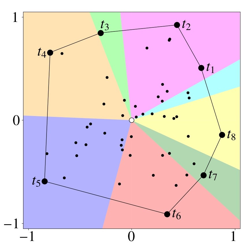
(a) Voronoi cells and IPDG

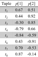
(b) Attribute values

Figure 1: Example of two-dimensional dataset

Figure 1 illustrates a point set $P$ in $\mathbb{R}^{2}$. The extreme points $X=\{t_{1},\ldots,t_{8}\}$ are highlighted and their Voronoi cells are filled with different colors in Figure 1(a). Note that an extreme point $t$ does not necessarily fall in its Voronoi cell, as another point $t^{\prime}$ may be top-ranked for vector $t$, i.e., $\langle t,t\rangle<\langle t^{\prime},t\rangle$. This explains why $t_{1}$ is not contained in $R(t_{1})$ (the cyan region) but in $R(t_{2})$ (the pink region). Figure 1(a) also illustrates the IPDG of the point set, where any two extreme points with adjacent Voronoi cells are connected.

3 Exact Algorithm in 2D

In this section, we present E-GRMR, our optimal polynomial-time algorithm for GRMR in $\mathbb{R}^{2}$. Before delving into the details, we first present some high-level ideas on the geometric properties of GRMR in $\mathbb{R}^{2}$ and our approach to solving it.

First of all, the set of all linear ranking functions in $\mathbb{R}^{2}$ corresponds to the one-dimensional unit sphere $\mathbb{S}^{1}$, i.e., the unit circle, and thus both exact and $\varepsilon$-approximate Voronoi cells correspond to arcs of $\mathbb{S}^{1}$. Therefore, GRMR in $\mathbb{R}^{2}$ can be equivalently formulated as the problem of finding the minimum number of arcs (cells) that fully cover $\mathbb{S}^{1}$. One straightforward approach to this problem is to first compute the $\varepsilon$-approximate Voronoi cells for an input parameter $\varepsilon$ and then solve the aforementioned covering problem. Then, we observe that the exact Voronoi cell of each extreme point can be computed via simple comparisons with its two neighbors in the IPDG (recall that the degree of each vertex in $\mathcal{G}(P)$ is $2$ when $d=2$). Moreover, computing an $\varepsilon$-approximate Voronoi cell of a point requires comparisons with merely extreme points. After the Voronoi cells are computed, the arc-covering problem is polynomial because it is one-dimensional. In the optimal algorithm we propose below, we further manages to avoid explicit computations of $\varepsilon$-approximate Voronoi cells and reduce the cost of the arc-covering problem via a graph-based transformation.

3.1 The E-GRMR Algorithm

The main idea behind E-GRMR is to build a directed graph $G$ such that each (directed) cycle corresponds to an $\varepsilon$-regret set. Then, the shortest cycle in $G$ provides an optimal solution for GRMR. The details of E-GRMR is shown in Algorithm 1. Note that, besides the database $P$ and parameter $\varepsilon$, the set $X$ of extreme points is also assumed to be given as input. For any given $P$, $X$ can be computed using any existing convex hull algorithm, such as Graham’s scan [19] and Qhull [8].

For ease of illustration, we arrange all points and vectors in a counterclockwise direction based on their corresponding angles from $0$ to $2\pi$ in the polar coordinate system. For a point $p\in\mathbb{R}^{2}$ or a vector $x\in\mathbb{R}^{2}$, we use ${\theta}(p)$ or ${\theta}(x)\in[0,2\pi)$ to denote the angle of $p$ or $x$, respectively. Furthermore, given any two points (vectors) $a,b\in\mathbb{R}^{2}$, we use $P[a,b]\subseteq P$ to denote a subset of points in $P$ whose angles are in range $[{\theta}(a),{\theta}(b)]$ if ${\theta}(a)<{\theta}(b)$ or ranges $[{\theta}(a),2\pi)$ and $[0,{\theta}(b)]$ if ${\theta}(a)>{\theta}(b)$.

Input : Database $P$, Extreme points $X\subseteq P$, Parameter $\varepsilon\in(0,1)$

Output : Optimal result $Q^{*}_{\varepsilon}$ of GRMR

1 for $i\leftarrow 1,\ldots,|X|$ do

2       Let $x^{*}_{i}$ be the vector $x\in\mathbb{S}^{1}$ s.t. $\langle t_{i},x\rangle=\langle t_{i+1},x\rangle\wedge\langle t_{i},x\rangle>0$;

3      

4Initialize the candidate set $S\leftarrow X$;

5 foreach point $p\in P\setminus X$ do

6       if $\exists i\in[|X|]:\langle p,x^{*}_{i}\rangle\geq(1-\varepsilon)\cdot\langle t_{i},x^{*}_{i}\rangle$ then

7             $S\leftarrow S\cup\{p\}$;

8            

9      

10Arrange all points of $S$ in a counterclockwise direction and index them by $[1,\ldots,|S|]$ accordingly;

11 Initialize a directed graph $G=(U,A)$ where $U=S$ and $A=\varnothing$;

12 foreach $i,j\in[|S|]$ and $i\neq j$ do

13       if $\angle s_{i}Os_{j}\geq\pi$ then continue;

14       $l_{ij}\leftarrow$ ComputeRegret$(s_{i},s_{j})$;

15       if $l_{ij}\leq\varepsilon$ then

16             Add a directed edge $(s_{i}\rightarrow s_{j})$ to $A$;

17            

18      

19$C^{*}\leftarrow$ ShortestCycle$(G)$;

20 return $Q^{*}_{\varepsilon}\leftarrow\{q:q\in C^{*}\}$;

21 Function ComputeRegret$(s_{i},s_{j})$

22       Find the subset of extreme points $X[s_{i},s_{j}]\subseteq X$;

23       Let $x^{*}$ be the vector $x\in\mathbb{S}^{1}$ s.t. $\langle s_{i},x\rangle=\langle s_{j},x\rangle\wedge\langle s_{i},x\rangle\geq 0$;

24       return $l_{ij}\leftarrow\max_{t\in X[s_{i},s_{j}]}\big{(}1-\frac{\langle s_{i},x^{*}\rangle}{\langle t,x^{*}\rangle}\big{)}$;

25      

Algorithm 1 E-GRMR

E-GRMR proceeds in three steps as follows.

Step 1 (Candidate Selection, Lines 1–1): The purpose of this step is to identify a subset $S\subseteq P$ of points that may be included in the solution, while pruning from consideration the points that are certainly not. To find the candidate points, E-GRMR essentially ignores all points that are never within an $(1-\varepsilon)$-approximation from a top-ranked point. In other words, $p\in S$ if and only if the $\varepsilon$-approximate Voronoi cell of $p$ is non-empty, i.e., $R_{\varepsilon}(p)\neq\varnothing$. Note that this condition holds for any extreme point in $X$. To determine whether it holds for a point $p\in P\setminus X$ or not, E-GRMR needs to find at least one vector $x\in R_{\varepsilon}(p)$ by comparing $p$ with each extreme point. In particular, for a point $p\in P\setminus X$ and an extreme point $t\in X$, it should decide if $R(t)\cap R_{\varepsilon}(p)$ is empty. To this end, it computes the minimum of the regret ratio of $p$ w.r.t. $t$ in $R(t)$. Indeed, this minimum is always reached at a boundary vector where the score of $t$ is equal to the score of the previous/next extreme point. The correctness of the above results will be analyzed in Section 3.2.

Putting everything together, E-GRMR first computes the boundary vector $x^{*}_{i}$ of $R(t_{i})$ and $R(t_{i+1})$ for each pair of neighboring extreme points $t_{i},t_{i+1}\in X$ (when $i=|X|$, $t_{|X|}$ and $t_{1}$ are used to compute $x^{*}_{|X|}$). Then, it checks the regret ratio of $p$ for each $x^{*}_{i}$ ($i\in[1,|X|]$) and adds $p$ to $S$ if its regret ratio is at most $\varepsilon$ for some $x^{*}_{i}$. Finally, all points in $S$ are arranged in a counterclockwise direction from $0$ to $2\pi$ and indexed by $[1,\ldots,|S|]$ accordingly.

Step 2 (Graph Construction, Lines 1–1): The purpose of this step is to identify each pair of points in $S$ that, if included in the solution, would make the points between them redundant (in the sense that the solution without these points is still an $\varepsilon$-regret set). This is achieved by building a directed graph $G=(U,A)$ as follows. First, $G$ includes all points in $S$ as vertices. For each two vertices $s_{i},s_{j}\in U$ ($i\neq j$), there will be a directed edge from $s_{i}$ to $s_{j}$ if the maximum regret ratio $l_{ij}$ caused by removing all points in $S$ between them (excluding themselves), i.e., $S[s_{i+1},s_{j-1}]$, is at most $\varepsilon$. Note that if the vector angle between $s_{i}$ and $s_{j}$ is greater than $\pi$, the regret led by removing points between them will be unbounded. In this case, the regret computation will be skipped directly.

The procedure to compute $l_{ij}$ is given in Lines 1–1. Firstly, it retrieves all extreme points $X[s_{i},s_{j}]$ between $s_{i}$ and $s_{j}$. If there is no extreme point in $X[s_{i},s_{j}]$ (other than $s_{i}$ or $s_{j}$ possibly), then it sets $l_{ij}=0$, leading to the inclusion of an edge from $s_{i}$ to $s_{j}$ for any $\varepsilon\geq 0$. Otherwise, to compute $l_{ij}$, it first finds the boundary vector $x^{*}$ where $s_{i}$ and $s_{j}$ have the same score. Similar to the case of candidate selection, the maximum of the regret ratio of $\{s_{i},s_{j}\}$ w.r.t. any extreme point $t$ between them is also always reached at the boundary vector $x^{*}$. Subsequently, it computes the regret ratio of $\{s_{i},s_{j}\}$ w.r.t. each extreme point $t\in X[s_{i},s_{j}]$ for vector $x^{*}$ and finally returns the maximum one as $l_{ij}$.

Step 3 (Result Computation, Lines 1–1): Given a directed graph $G=(U,A)$ constructed according to the above procedure, the final step is to find the shortest cycle $C^{*}$ of $G$ and return the vertices of $C^{*}$ as the optimal result $Q^{*}_{\varepsilon}$ of GRMR on database $P$. In our implementation, we run Dijkstra’s algorithm [15] from each vertex of $G$ to find the shortest cycle $C^{*}$.

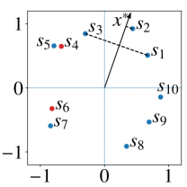
(a) Candidate set $S$

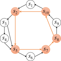
(b) Graph $G$ for $\varepsilon=0.1$

Figure 2: Example for E-GRMR in 2D

Example 1.

We give an example of Algorithm 1 in Figure 2. In Figure 2(a), we illustrate the candidate set $S$ for $\varepsilon=0.1$ extracted from the point set in Figure 1(a). The extreme points (resp. $t_{1}$–$t_{8}$ in Figure 1(b)) are blue and the remaining two candidates ($s_{4}=(-0.67,0.65)$ and $s_{6}=(-0.82,-0.32)$) are red. We also show how to compute $l_{13}$ for $s_{1}$ and $s_{3}$ in Figure 2(a). First of all, the boundary vector $x^{*}=(0.34,0.97)$ with $\langle s_{1},x^{*}\rangle=\langle s_{3},x^{*}\rangle$ is found. Then, the regret ratio of $\{s_{1},s_{3}\}$ over $s_{2}$ for $x^{*}$ is computed as $l_{13}$. Since $l_{13}\approx 0.3>0.1$, the edge $(s_{1}\rightarrow s_{3})$ is not added to $G$. The graph $G$ constructed for $\varepsilon=0.1$ is shown in Figure 2(b). The shortest cycle $C^{*}$ of $G$ is highlighted in orange and $Q^{*}_{0.1}=\{s_{2},s_{5},s_{7},s_{8},s_{10}\}$ is the optimal result of GRMR for $\varepsilon=0.1$.

3.2 Theoretical Analysis

Next, we will analyze the correctness and time complexity of Algorithm 1 theoretically. The road map of our analysis is as follows. Firstly, Lemma 1 shows the validity of candidate selection. Secondly, Lemma 2 proves the correctness of regret computation and graph construction. Thirdly, Lemma 3 states the equivalence between computing the optimal result of GRMR on $P$ and finding the shortest cycle in $G$. Combining Lemmas 1–3, we prove the optimality of Algorithm 1 in Theorem 2. Finally, we analyze the time complexity of Algorithm 1 in Theorem 3.

Lemma 1.

A point $p\in S$ if and only if $R_{\varepsilon}\neq\varnothing$.

Lemma 2.

For any $s_{i},s_{j}\in S$ ($i<j$), the maximum regret ratio of $\{s_{i},s_{j}\}$ after removing all points in $S$ between them is at most $l_{ij}$.

Lemma 3.

If $C$ is a cycle of $G$, then $Q=\{q:q\in C\}$ is an $\varepsilon$-regret set of $P$; If $Q$ is a locally minimal $\varepsilon$-regret set of $P$, then there exists a cycle $C$ of $G$ corresponding to $Q$.

Please refer to Appendix B–D for the proofs of Lemma 1-3.

Theorem 2.

The result $Q^{*}_{\varepsilon}$ returned by Algorithm 1 is optimal for GRMR with parameter $\varepsilon$ on database $P$.

Proof.

Based on Lemma 1, Algorithm 1 excludes all redundant points from computation. According to Lemmas 2 and 3, it is guaranteed that any locally minimal $\varepsilon$-regret set of $P$ forms a cycle in $G$. Therefore, the optimal result $Q^{*}_{\varepsilon}$ of GRMR on $P$, i.e., the smallest $\varepsilon$-regret set of $P$, must correspond to the shortest cycle of $G$. Hence, we conclude that Algorithm 1 is optimal for GRMR in $\mathbb{R}^{2}$. ∎

Theorem 3.

The time complexity of Algorithm 1 is $O(n^{3})$.

Proof.

Firstly, the time complexity of candidate selection is $O(|X|+n\cdot\log{|X|})$. Here, a binary search can be used to find the index $i$ and thus it takes $O(\log{|X|})$ time to decide whether $p$ is added to $S$ or not. Secondly, the time complexity of graph construction is $O(|S|^{2}\cdot|X|)$. Thirdly, the time complexity of finding the shortest cycle in a directed graph is $O(|U|\cdot|A|+|U|^{2}\cdot\log{|U|})$ when the variant of Dijkstra’s algorithm in [18] is used for computing the shortest path from each vertex. Recently, an $O(|U|\cdot|A|)$ time algorithm [30] has also been proposed for finding the shortest directed cycle. In the worst case (i.e., $\varepsilon$ is close to $1$), since $|S|=|U|=O(n)$ and $|A|=O(|S|^{2})$, the time complexity of Algorithm 1 is $O(n^{3})$. Nevertheless, if $\varepsilon$ is far away from $1$, it typically holds that $|S|=|U|\ll O(n)$ and $|A|=O(|U|)$. In this case, the time complexity of Algorithm 1 is $O(n\cdot\log{|X|}+|S|^{2}\cdot|X|)$. ∎

4 Heuristic Algorithm in HD

In the case of $d\geq 3$, GRMR becomes much more challenging (see Theorem 1). Let us first highlight some challenges of GRMR in HD. Firstly, as discussed in Section 2.2, GRMR can be seen as a geometric set-cover problem. Solving it directly as such will require the invocation of set operations between Voronoi cells. However, the geometric shapes of Voronoi cells in high dimensions are convex cones defined by intersections of half-spaces, and set operations on Voronoi cells become very inefficient. Secondly, constructing the IPDG exactly is also computationally intensive when $d\geq 3$, as the number of edges in the IPDG grows exponentially with $d$. Thirdly, even when the Voronoi cells and IPDG of a database are given as inputs, finding the optimal solution of GRMR is still infeasible unless P=NP due to the combinatorial complexity of geometric covering problems in two or higher dimensions [17].

To devise a practical heuristic that addresses the above issues, we adopt two major simplifications in relation to GRMR. First, we only consider solutions that are subsets of the extreme points $X$ instead of the entire database. Empirically, this does not significantly degrade the solution quality, as the optimal result of GRMR is often a subset of $X$. Secondly, when considering an extreme point $t\in X$ for the solution set, we restrict ourselves to merely two possibilities: either $t$ is in the solution; or there exists an extreme point $t^{\prime}$ in the solution whose $\varepsilon$-approximate Voronoi cell can fully cover the Voronoi cell of $t$, in which case we say that $t^{\prime}$ dominates $t$. In other words, we do not consider the case that $R(t)$ is covered by a union of the $\varepsilon$-approximate Voronoi cells of two or more points, because computing the union is very inefficient. The above simplifications allow us to develop an approach that can be expressed in terms of a graph structure, to which we refer as the dominance graph, because it encapsulates information about the dominance relationships among vertices. The resulting approach can be seen as targeting a simplified formulation of the original GRMR problem.

In what follows, we first describe the dominance graph and how we obtain a simplified problem formulation from it in Section 4.1. Subsequently, in Section 4.2, we describe H-GRMR, an efficient heuristic algorithm for GRMR on databases of arbitrary dimensionality, and analyze its properties. Finally, we discuss some issues on the practical implementation of H-GRMR in Section 4.3.

4.1 Dominance Graph

Let the points in $X$ be indexed by $[1,\ldots,|X|]$ as $\{t_{1},t_{2},\ldots,t_{|X|}\}$. The dominance graph $\mathcal{H}=(V,E)$ is a directed weighted graph where $V$ is the set $X$ of extreme points. A directed edge $(t_{i}\rightarrow t_{j})$ with an associated weight $\varepsilon_{ij}\in(0,1)$ exists if and only if the $\varepsilon_{ij}$-approximate Voronoi cell of $t_{i}$ fully covers the Voronoi cell of $t_{j}$. Therefore, the presence of edge $(t_{i}\rightarrow t_{j})$ signifies that, in any solution of GRMR with $\varepsilon\geq\varepsilon_{ij}$, $t_{i}$ can replace $t_{j}$ without a violation of the regret constraint.

The edge weight $\varepsilon_{ij}$ for each pair of points $t_{i},t_{j}$ can be computed from the linear program (LP) in Eq. 1.

$$\begin{aligned} \text{Maximize:}\quad&1-t_{i}^{\top}x\\ \text{Subject to:}\quad&(t_{j}-t)^{\top}x\geq 0,\forall t\in N(t_{j})\\ &t_{j}^{\top}x=1\end{aligned}$$ (1)

In Eq. 1, $N(t)$ is the set of neighbors of $t$ in $\mathcal{G}(P)$, i.e., the set of extreme points whose Voronoi cells are adjacent to $R(t)$. The first set of inequality constraints means that the feasible region of the linear program is the Voronoi cell $R(t_{j})$ of $t_{j}$, which is defined by the intersections of $|N(t_{j})|$ closed half-spaces. Each half-space corresponds to the region where the score of $t_{j}$ is greater than or equal to that of $t\in N(t_{j})$. Hence, $\langle t_{j},x\rangle\geq\langle t,x\rangle\;\Leftrightarrow\;(t_{j}-t)^{\top}x\geq 0$. The second constraint normalizes the score of $t_{j}$ to be $1$. Under this constraint, for a given vector $x$, the regret ratio of $t_{i}$ w.r.t. $t_{j}$ is equal to $1-t_{i}^{\top}x$. The LP in Eq. 1 finds the maximum regret ratio $\varepsilon_{ij}$ of $t_{i}$ w.r.t. $t_{j}$ over the feasible region, i.e., $R(t_{j})$.

After the dominance graph $\mathcal{H}$ is built, one can use it to compute a (possibly suboptimal) solution of GRMR. In particular, for a parameter $\varepsilon\in(0,1)$, an $\varepsilon$-regret set can be obtained as any subset $S\subseteq X$ of points that satisfies the following condition: for each $t_{j}\in X$, either $t_{j}\in S$ or there exists an edge $(t_{i}\rightarrow t_{j})$ with $\varepsilon_{ij}\leq\varepsilon$ for some $t_{i}\in S$. Let $\mathcal{H}_{\varepsilon}=(V,E_{\varepsilon})$ be the subgraph of $\mathcal{H}$ where $V=X$ and $E_{\varepsilon}\subseteq E$ is a subset of edges with weights at most $\varepsilon$. Then, a heuristic solution of GRMR can be obtained by finding the minimum dominating set of $\mathcal{H}_{\varepsilon}$.

4.2 The H-GRMR Algorithm

The H-GRMR algorithm proceeds in two steps as presented in Algorithms 2 and 3.

Input : Extreme points $X\subseteq P$, IPDG $\mathcal{G}(P)$, Parameter $\varepsilon$

Output : Dominance graph $\mathcal{H}_{\varepsilon}$

1 Initialize a directed graph $\mathcal{H}_{\varepsilon}=(V,E_{\varepsilon})$ where $V=X$ and $E_{\varepsilon}=\varnothing$;

2 for $i\leftarrow 1,\ldots,|X|$ do

3       Initialize an empty queue $\mathcal{Q}$;

4       foreach $t\in N(t_{i})$ do $\mathcal{Q}$.enqueue$(t)$;

5       Set $t_{i}$ as visited;

6       while $\mathcal{Q}$ is not empty do

7             $t_{j}\leftarrow\mathcal{Q}$.dequeue();

8             if $t_{j}$ is not visited then

9                   Set $t_{j}$ as visited;

10                   Solve LP in Eq. 1 for $t_{i},t_{j}$ to compute $\varepsilon_{ij}$;

11                   if $\varepsilon_{ij}\leq\varepsilon$ then

12                         Add a directed edge $(t_{i}\rightarrow t_{j})$ to $E_{\varepsilon}$;

13                         foreach $t\in N(t_{j})$ do $\mathcal{Q}$.enqueue$(t)$;

14                        

15                  

16            

17      

18return $\mathcal{H}_{\varepsilon}$;

Algorithm 2 BuildDomGraph

Step 1 (Dominance Graph Construction, Algorithm 2): As discussed above, for a parameter $\varepsilon\in(0,1)$, we only need to build a subgraph $\mathcal{H}_{\varepsilon}$ of the dominance graph $\mathcal{H}$ to compute a solution of GRMR. The procedure to build $\mathcal{H}_{\varepsilon}$ is described in Algorithm 2. It assumes that the IPDG $\mathcal{G}(P)$ is provided as an input, and in Section 4.3 we will discuss a practical alternative to this assumption. Generally, it performs a breadth-first search (BFS) on $\mathcal{G}(P)$ starting from each vertex $t_{i}\in X$. For a starting vertex $t_{i}$, when the BFS encounters another vertex $t_{j}$, the LP in Eq. 1 is solved to compute the weight $\varepsilon_{ij}$ from $t_{i}$ to $t_{j}$. If $\varepsilon_{ij}\leq\varepsilon$, it will add an edge $(t_{i}\rightarrow t_{j})$ to $E_{\varepsilon}$ and continue to traverse the neighbors of $t_{j}$ in $\mathcal{G}(P)$. Otherwise, the BFS does not expand to the neighbors of $t_{j}$ anymore. This is because vertices with higher inner-product similarities (resp. lower weights) tend to be closer to each other in the IPDG and stopping the BFS expansion early allows us to reduce the number of LP computations with little loss of solution quality.

Input : Database $P$, Extreme points $X$, IPDG $\mathcal{G}(P)$, Parameter $\varepsilon$

Output : Result $Q_{\varepsilon}$ of GRMR

1 $\mathcal{H}_{\varepsilon}\leftarrow$ BuildDomGraph ($X,\mathcal{G}(P),\varepsilon$);

2 Initialize $Q_{\varepsilon}\leftarrow\varnothing$ and $\mathcal{U}\leftarrow X$;

3 for $i\leftarrow 1,\ldots,|X|$ do

4       $Dom(t_{i})\leftarrow\{t_{i}\}\cup\{t_{j}\in X:(t_{i}\rightarrow t_{j})\in E_{\varepsilon}\}$;

5      

6while $\mathcal{U}\neq\varnothing$ do

7       $t^{*}\leftarrow\arg\max_{t_{i}\in X\setminus Q_{\varepsilon}}|Dom(t_{i})\cap\mathcal{U}|$;

8       $Q_{\varepsilon}\leftarrow Q_{\varepsilon}\cup\{t^{*}\}$ and $\mathcal{U}\leftarrow\mathcal{U}\setminus Dom(t^{*})$;

9      

10return $Q_{\varepsilon}$;

Algorithm 3 H-GRMR

Step 2 (Result Computation, Algorithm 3): After building $\mathcal{H}_{\varepsilon}$ using Algorithm 2, H-GRMR approaches the dominating set problem on $\mathcal{H}_{\varepsilon}$ as an equivalent set-cover problem on a set system $\Sigma=(\mathcal{U},\mathcal{S})$ where $\mathcal{U}$ is equal to $X$ and $\mathcal{S}$ is a collection of sets, with the $i$^th set equal to all points $Dom(t_{i})$ dominated by $t_{i}$, i.e., $Dom(t_{i})\coloneqq\{t_{i}\}\cup\{t_{j}:(t_{i}\rightarrow t_{j})\in\mathcal{H}_{\varepsilon}\}$. Then, it runs the greedy algorithm to compute an approximate set-cover solution on $\Sigma$. Specifically, starting from $Q_{\varepsilon}=\varnothing$, it adds a vertex whose dominating set contains the most number of uncovered vertices at each iteration until all vertices in $\mathcal{U}$ are covered. Finally, $Q_{\varepsilon}$ is returned as the solution of GRMR on database $P$.

Example 2.

Figure 3(a) illustrates the dominance graph $\mathcal{H}$ of the dataset in Figure 1. Then, in Figure 3(b), we show how $\mathcal{H}$ can be used to compute the solution of GRMR for $\varepsilon=0.2$. Specifically, $\mathcal{H}_{0.2}$ is a subgraph of $\mathcal{H}$ where only the edges with weights at most $0.2$ are preserved (deleted edges are in gray). Then, H-GRMR runs the greedy algorithm on $\mathcal{H}_{0.2}$ to compute the smallest dominating set. At the first iteration, $t_{8}$ is added to $Q_{0.2}$ because $|Dom(t_{8})|=3$ is the maximum among all vertices. Then, $t_{4}$ is added at the second iteration. Next, $t_{2},t_{5},t_{6}$ are added accordingly. Finally, the dominating set $Q=\{t_{2},t_{4},t_{5},t_{6},t_{8}\}$ of $\mathcal{H}_{0.2}$ provides a heuristic solution of GRMR for $\varepsilon=0.2$.

Theoretical Analysis: The result $Q_{\varepsilon}$ returned by Algorithm 3 is guaranteed not to break the regret constraint of GRMR, even if it may not be the smallest possible solution.

Theorem 4.

It holds that $Q_{\varepsilon}$ returned by Algorithm 3 is an $\varepsilon$-regret set of $P$, i.e., $l(Q_{\varepsilon})\leq\varepsilon$.

Proof.

For any vector $x\in\mathbb{S}^{d-1}$, there exists a point $t_{j}$ such that $x\in R(t_{j})$. Since $Q_{\varepsilon}$ is a dominating set of $G_{\varepsilon}$, we have either $t_{j}\in Q_{\varepsilon}$ or there exists an edge $(t_{i}\rightarrow t_{j})\in E_{\varepsilon}$ for some $t_{i}\in Q_{\varepsilon}$. In the previous case, we have $l_{x}(Q_{\varepsilon})=0$; In the latter case, we have $l_{x}(Q_{\varepsilon})\leq\varepsilon_{ij}\leq\varepsilon$. In both cases, we have $l(Q_{\varepsilon})\leq\varepsilon$. ∎

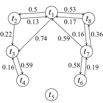
(a) Dominance graph $\mathcal{H}$

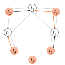
(b) Subgraph $\mathcal{H}_{0.2}$ for $\varepsilon=0.2$

Figure 3: Example of dominance graph and H-GRMR

How large is the size of the solution of H-GRMR compared to the size of the optimal solution for GRMR? While the approximation factor of H-GRMR on the solution size is still an open problem, we do have an upper bound for it.

Theorem 5.

If $Q_{\varepsilon}^{*}$ is the optimal solution of GRMR with parameter $\varepsilon$ and $Q_{\varepsilon}$ is the solution of GRMR returned by H-GRMR, then it holds that $|Q_{\varepsilon}|\leq\frac{|X|}{d+1}\cdot|Q_{\varepsilon}^{*}|$.

Proof.

First, the size of $Q_{\varepsilon}$ is at most $|X|$ since $Q_{\varepsilon}\subseteq X$. Second, $Q^{*}_{\varepsilon}$ must contain at least $d+1$ points to guarantee $l(Q^{*}_{\varepsilon})<1$. This is because, for any point set $Q$ of size $d$ in $\mathbb{R}^{d}$, we can find a vector $x$ perpendicular to the hyperplane containing all points in $Q$ such that $l_{x}(Q)=1$. Thus, $|Q_{\varepsilon}|\leq\frac{|X|}{d+1}\cdot|Q^{*}_{\varepsilon}|$. ∎

Next, we prove that H-GRMR is a polynomial-time algorithm.

Theorem 6.

The time complexity of H-GRMR is $O(|X|^{2}\cdot(\Delta\cdot d^{3.5}+\Gamma))$ where $\Delta=\max_{t\in X}|N(t)|$ and $\Gamma=\max_{t\in X}Dom(t)$.

Proof.

First of all, the number of LPs solved by BuildDomGraph is $O(|X|^{2})$, as the worst-case corresponds to computing the weight for each pair of vertices. Each LP in Eq. 1 has $|N(t_{j})|+1$ constraints and $d$ variables. When the interior point method is used as the LP solver, a worst-case time complexity of $O(\Delta\cdot d^{3.5})$ can always be guaranteed. Therefore, the time complexity of BuildDomGraph is $O(|X|^{2}\cdot\Delta\cdot d^{3.5})$. Then, the time to build the set system $\Sigma$ is $O(|X|\cdot\Gamma)$ where $\Gamma=\max_{t\in X}Dom(t)$. The greedy algorithm should evaluate the union of $Dom(t)$ and $\mathcal{U}$ for each $t\in X$ at each iteration. Thus, the running time of each iteration is $O(|X|\cdot\Gamma)$. Then, it runs $|Q_{\varepsilon}|=O(|X|)$ iterations. Hence, the time complexity of result computation is $O(|X|^{2}\cdot\Gamma)$. We conclude the proof by summing up both results. ∎

4.3 Practical Implementation

Next, we discuss practical aspects of the implementation of H-GRMR. The first one is how to build an approximate IPDG $\widehat{\mathcal{G}}(P)$. The second one is how to reuse the dominance graph for achieving better solution quality.

IPDG Construction: A naïve method to construct an exact IPDG $\mathcal{G}(P)$ for a point set $P\subset\mathbb{R}^{d}$ is to compute $\mathcal{CH}(P)$ and enumerate all edges of $\mathcal{CH}(P)$. Then, an edge of $\mathcal{CH}(P)$ corresponds to an edge of $\mathcal{G}(P)$ [48]. Although this method is practically efficient in $\mathbb{R}^{2}$ or even $\mathbb{R}^{3}$, it quickly becomes computationally intensive for higher dimensionality. One alternative approach we considered was based on existing works on graph-based maximum inner product search [27, 38, 48], which propose to build a graph analogous to IPDG. However, since graphs built by these methods are significantly different from the original IPDG, e.g., they are directed graphs and contain non-extreme points, it is not reasonable to use them for our problems directly.

Input : Extreme points $X$, Sample size $m$, Parameter $k$

Output : Approximate IPDG $\widehat{\mathcal{G}}(P)$

1 Initialize an undirected graph $G=(V,E)$ where $V=X$ and $E=\varnothing$;

2 for $i\leftarrow 1,\ldots,m$ do

3       Draw a random vector $x_{i}$ uniformly from $\mathbb{S}^{d-1}$;

4       Compute the top-$k$ results $\Phi_{k}(x_{i},X)$ for $x_{i}$ in $X$;

5       Let $t^{*}$ be the top-ranked tuple for $x_{i}$ in $X$;

6       foreach $t\in\Phi_{k}(x_{i},X)$ and $t\neq t^{*}$ do

7             Add an undirected edge $\{t^{*},t\}$ to $E$;

8            

9      

10return $\widehat{\mathcal{G}}(P)\leftarrow G$;

Algorithm 4 IPDG Construction

Instead, we propose a new method to build an approximate IPDG as described in Algorithm 4. Our method is based on an intuitive observation: if the Voronoi cells of two points $t,t^{\prime}$ are adjacent, then there is some vector in $R(t)$ for which $t^{\prime}$ is high-ranked, i.e., $t^{\prime}$ is among the top-$k$ results for a small $k$ – and vice versa. We use this observation in Algorithm 4 as follows. First, we draw $m$ random vectors from $\mathbb{S}^{d-1}$. Then, we compute the top-$k$ results $\Phi_{k}(x_{i},X)$ for each sampled vector $x_{i}$. Subsequently, we identify the top-ranked point $t^{*}$ from $\Phi_{k}(x_{i},X)$ and add the edges between $t^{*}$ and the remaining points in $\Phi_{k}(x_{i},X)$. Finally, the resultant graph after processing all sampled vectors are returned as $\widehat{\mathcal{G}}(P)$.

We note that using an approximate IPDG $\widehat{\mathcal{G}}(P)$ instead of the exact one $\mathcal{G}(P)$ does not affect the correctness of H-GRMR, i.e., the solution returned by H-GRMR is still an $\varepsilon$-regret set. Compared with $\mathcal{G}(P)$, $\widehat{\mathcal{G}}(P)$ may both contain some additional edges and miss some existing edges. On the one hand, an additional edge has no effect on the result of the LP in Eq. 1. This is because its feasible region is exactly the Voronoi cell $R(t_{j})$ of $t_{j}$. Hence, an additional edge leads to a redundant constraint that does not reduce the feasible region at all. On the other hand, a missing edge may cause that the result the LP in Eq. 1 is larger than the optimal maximum regret ratio, because the feasible region is larger than $R(t_{j})$. As a result, $\mathcal{H}_{\varepsilon}$ may contain fewer edges and the solution $Q_{\varepsilon}$ may have more points. Nevertheless, $Q_{\varepsilon}$ is still guaranteed to be an $\varepsilon$-regret set. Therefore, the values of $k$ and $m$ can affect the performance of H-GRMR by controlling the number of edges in $\widehat{\mathcal{G}}(P)$. When larger values of $k$ and $m$ are used, $\widehat{\mathcal{G}}(P)$ will contain more edges in $\mathcal{G}(P)$ and $Q_{\varepsilon}$ will be smaller. At the same time, larger values of $k$ and $m$ will also lead to more additional edges in $\widehat{\mathcal{G}}(P)$ and thus a lower efficiency of dominance graph construction.

Graph Reuse: In H-GRMR, we build a graph $\mathcal{H}_{\varepsilon}$ that only contains edges with weights at most $\varepsilon$ for computation. In fact, it is possible to use $\mathcal{H}_{\varepsilon}$ for GRMR with any $\varepsilon^{\prime}\in(0,\varepsilon)$ since one can extract a subgraph $\mathcal{H}_{\varepsilon^{\prime}}$ from $\mathcal{H}_{\varepsilon}$ by deleting the edges with weights greater than $\varepsilon^{\prime}$. Then, the dominating set of $\mathcal{H}_{\varepsilon^{\prime}}$ is also the result $Q_{\varepsilon^{\prime}}$ for GRMR with parameter $\varepsilon^{\prime}$. In light of this observation, we devise an approach to improving the solution quality of H-GRMR.

As discussed already, H-GRMR returns an $\varepsilon$-regret set that may not have the minimum size. To explore solutions of smaller size than the one returned by H-GRMR, we invoke it with a larger parameter, and by doing so, we reuse previously materialized instances of $\mathcal{H}$ as much as possible. Specifically, given a parameter $\varepsilon\in(0,1)$, we first build a graph $\mathcal{H}_{\eta}$ for some $\eta>\varepsilon$. Then, we perform a binary search on $\delta$ in the range $[\varepsilon,\eta]$, and for each value of $\delta$, obtain a solution $Q_{\delta}$ by invoking H-GRMR with parameter $\delta$, while reusing $\mathcal{H}_{\eta}$ as described above. The goal of the binary search is to find the maximum value of $\delta$ that satisfies the regret constraint of GRMR, i.e., $l(Q_{\delta})\leq\varepsilon$, and return $Q_{\delta}$ for GRMR with parameter $\varepsilon$. In practice, we observe that the size of $Q_{\delta}$ is smaller than the size of $Q_{\varepsilon}$ we would obtain by a single invocation of H-GRMR for the input parameter. In practice, for small values of $\varepsilon$, setting $\eta=3\cdot\varepsilon$ is good enough in almost all cases. With the incorporated binary search, the time complexity of H-GRMR increases to $O(|X|^{2}\cdot(\Delta\cdot d^{3.5}+\Gamma\cdot\log{\frac{1}{\varepsilon}}))$, since the result computation procedure is repeated $O(\log{\frac{1}{\varepsilon}})$ times for the binary search on the value of $\delta$.

Similar approach can also be used for the dual formulation of GRMR in Section 2.1. By building $\mathcal{H}$ and performing a binary search on $\delta\in(0,1)$, we can find the minimum value of $\delta$ that guarantees $|Q_{\delta}|\leq r$ and return $Q_{\delta}$ as the result for the dual problem.

5 Experiments

In this section, we evaluate the performance of our algorithms on real and synthetic datasets. We first introduce our experimental setup in Section 5.1. Then, we present the experimental results on two-dimensional datasets in Section 5.2. Finally, the experimental results on high-dimensional datasets are reported in Section 5.3.

5.1 Experimental Setup

Implementation: We conduct all experiments on a server running Ubuntu 18.04.1 with a 2.3GHz processor and 256GB memory. All algorithms are implemented in C++11. We use GLPK as the LP solver. The implementation is published on GitHub.

Table 1: Statistics of Real Datasets

Dataset	Size	Dimension	Source
Airline	1,700,782	2	DOT
NBA	24,585	2	Kaggle
Climate	566,262	6	CRU
El Nino	178,080	5	UCI
Household	2,049,280	7	UCI
SUSY	5,000,000	8	UCI

Real Datasets: We use six publicly available real datasets for evaluation. Basic statistics of these datasets are listed in Table 1.

• Airline: It records the information of all flights conducted by US carriers from January 2019 to March 2019. We used two attributes, i.e., arrival delay and air-time, for evaluation.

• NBA: It contains the statistics of NBA players aggregated by season/team. We used two attributes, i.e., offensive win shares (ows) and defensive win shares (dws), for evaluation.

• Climate: It contains the climate information of different locations. We used six attributes in our experiments, including (annual average) temperature and humidity.

• El Nino: It contains oceanographic data in the Pacific ocean. We used all five numerical attributes for evaluation.

• Household: It contains the electric power consumption measurements gathered in a household. We used all seven numerical attributes for evaluation.

• SUSY: A high-energy physics dataset that contains eight numerical features, representing kinematic properties measured by particle detectors.

We normalized all attribute values of each dataset to the range $[-1,1]$ in the preprocessing step.

Synthetic Datasets: To evaluate the performance of different algorithms in controlled settings, we use two synthetic datasets, namely Normal and Uniform, in our experiments. In the Normal dataset, each attribute is independently drawn from the standard normal distribution $\mathcal{N}(0,1)$. In the Uniform dataset, each attribute is independently drawn from a uniform distribution $\mathcal{U}(-1,1)$. For both datasets, we vary the number of tuples $n$ from $10^{4}$ ($10$k) to $10^{7}$ ($10$m) and the dimensionality $d$ from $2$ to $10$ for testing the performance of different algorithms with varying $n$ and $d$. By default, we use the dataset with $n=10^{6}$ ($1$m) and $d=6$.

Algorithms: We compare the following eight algorithms for GRMR in our experiments.

• $\varepsilon$-Kernel [1]: We use the ANN-based algorithm to compute an $\varepsilon$-kernel as the result of GRMR. The approach is a straightforward adaptation of the analysis in [1] and returns an $\varepsilon$-regret set of size $O(\frac{1}{\varepsilon^{(d-1)/2}})$ for GRMR.

• HittingSet [2] for RMS can be used for GRMR by extending the sample space of ranking functions from monotonic linear to general linear functions (i.e., sampling vectors from $\mathbb{S}^{d-1}$ instead of $\mathbb{S}^{d-1}_{+}$) based on the $\varepsilon$-net property. It returns an $\varepsilon$-regret set of size $O(|Q^{*}_{\varepsilon}|\cdot\log{|Q^{*}_{\varepsilon}|})$ where $Q^{*}_{\varepsilon}$ is the optimal solution of GRMR.

• 2D-RRMS [3] is an exact algorithm for RMS in $\mathbb{R}^{2}$.

• Greedy [28], HD-RRMS [3], and Sphere [41] are typical (approximate/heuristic) algorithms for RMS in $\mathbb{R}^{d}$ when $d\geq 3$.

• E-GRMR is our exact algorithm for GRMR in $\mathbb{R}^{2}$ (Section 3).

• H-GRMR is our heuristic algorithm for GRMR in $\mathbb{R}^{d}$ (Section 4).

Theoretically, the sampling complexities of $\varepsilon$-Kernel and HittingSet are $O(\frac{1}{\varepsilon^{(d-1)/2}})$ and $O(\frac{1}{\varepsilon^{d-1}})$, respectively, which makes them impractical in high dimensions. In our implementation, rather than performing the sampling all at once, we sample them in stages and maintain a result $Q$ based on the current samples until $l(Q)\leq\varepsilon$. Moreover, the RMS algorithms, i.e., 2D-RRMS, Greedy, HD-RRMS, and Sphere, cannot be directly used for GRMR because they only consider monotonic linear functions, but not ones with negative weights. In practice, we cast a GRMR problem into $2^{d}$ RMS problems by dividing the points in a dataset into the standard $2^{d}$ orthants. We then run an RMS algorithm on each partition (resp. each orthant) and return the union of results for GRMR. Note that this method has no theoretical guarantees, and empirically it often fails to provide a valid $\varepsilon$-regret set when the points are not evenly distributed among orthants. Nevertheless, we could not find in the literature any other approach to adapting them to GRMR. Finally, the set of extreme points (or the skylines of all partitions for RMS algorithms) on each dataset is precomputed and provided as an input to all algorithms.

Performance Measures: The efficiency of each algorithm is measured by running time, i.e., the CPU time to compute the result of GRMR for a given $\varepsilon$. The quality of a result $Q$ is measured by the maximum regret ratio $l(Q)$, as well as its size $|Q|$ for a given $\varepsilon$. Among all solutions satisfying $l(Q)\leq\varepsilon$, the one with a smaller size is considered better. To estimate the maximum regret ratio, we draw a set of $10^{6}$ random vectors from $\mathbb{S}^{d-1}$, compute the regret ratio of $Q$ for each vector, and use the maximum one as an estimate for $l(Q)$. For a given dataset, we run each algorithm $10$ times and take the averages of these measures for evaluation.

5.2 Results on Two-Dimensional Datasets

In this subsection, we focus on the two-dimensional datasets and compare the performance of our proposed algorithms E-GRMR and H-GRMR with algorithms tailored to two-dimensional settings, i.e., $\varepsilon$-Kernel, HittingSet, and 2D-RRMS. We present the results for two real datasets (Airline and NBA) and one synthetic dataset (Normal). Since the results for Uniform are similar to those for Normal in 2D, we omit them due to space limitations.

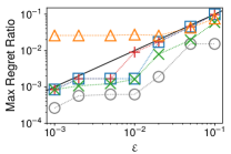
(a) Airline

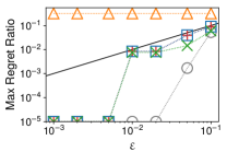
(b) NBA

Figure 4: Parameter $\varepsilon$ vs. max regret ratio

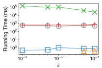
(a) Airline

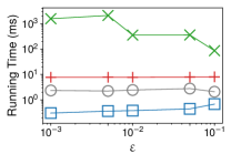
(b) NBA

Figure 5: Running time with varying $\varepsilon$

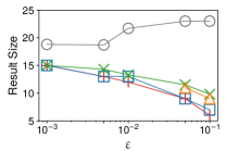
(a) Airline

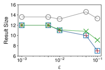
(b) NBA

Figure 6: Result sizes with varying $\varepsilon$

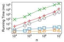
(a) Normal (2D)

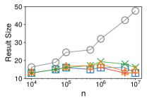
(b) Normal (2D)

Figure 7: Performance with varying $n$ ($\varepsilon=0.01$)

Impact of Parameter $\varepsilon$: We vary $\varepsilon$ from $0.001$ to $0.1$ to evaluate the effect of $\varepsilon$ on the performance of each algorithm. Figure 6 illustrates the maximum regret ratio $l(Q)$ of the result $Q$ of each algorithm for different $\varepsilon$ on Airline and NBA. Note that GRMR requires that $l(Q)\leq\varepsilon$, and so valid results should map below the line $l(Q)=\varepsilon$ in Figure 6. We observe that all algorithms except 2D-RRMS can always guarantee to provide an $\varepsilon$-regret set. 2D-RRMS fails to provide valid results in most cases because casting GRMR in 2D into $4$ RMS subproblems does not work well in the case that the data points are not evenly distributed among orthants.

The running time and result sizes of each algorithm with varying $\varepsilon$ are presented in Figures 6 and 6, respectively. First of all, the running time of E-GRMR is stable with increasing $\varepsilon$. This is because E-GRMR spends over $95\%$ of CPU time on candidate selection, whose time complexity is independent of $\varepsilon$. Since the size of the candidate set is much smaller than the size of the dataset, the time for graph construction and result computation is nearly negligible compared with that for candidate selection. Then, as expected, the result size of E-GRMR decreases with $\varepsilon$ and is always the smallest (optimal) one among all algorithms. However, E-GRMR only outperforms HittingSet in terms of efficiency. On the other hand, H-GRMR runs one to four orders of magnitude faster than all other algorithms (except 2D-RRMS that cannot provide valid results in most cases). At the same time, we observe empirically that H-GRMR often provides the optimal or near-optimal results for GRMR, because of the optimality of Delaunay graphs in $\mathbb{R}^{2}$ and the effectiveness of the dominance graph for GRMR.

Impact of Dataset Size $n$: Subsequently, we fix $\varepsilon=0.01$ and vary the size $n$ of Normal from $10^{4}$ to $10^{7}$. The performance of each algorithm is shown in Figure 7. First of all, the running time of $\varepsilon$-Kernel, E-GRMR, and HittingSet increases linearly with $n$ since their time complexities are all linear with $n$. 2D-RRMS and H-GRMR show much better scalability w.r.t. $n$ because they only use the skyline and extreme points for computation, whose sizes are much smaller than $n$ and increase sub-linearly with $n$. Furthermore, the solution quality of $\varepsilon$-Kernel is significantly inferior to all other algorithms, especially when $n$ is larger, because the ANN-based method does not consider whether the $\varepsilon$-kernel is the smallest or not. Conversely, our proposed algorithms as well as HittingSet and 2D-RRMS prefer smaller results to larger ones. 2D-RRMS can provide valid results on Normal because the data points are almost evenly distributed among four orthants.

In general, E-GRMR always returns the optimal results of GRMR within reasonable time while H-GRMR provides near-optimal results of GRMR with superior efficiency on all 2D datasets for different values of $\varepsilon$ and $n$.

5.3 Results on High-Dimensional Datasets

In this subsection, we compare the performance of H-GRMR with $\varepsilon$-Kernel, HittingSet, and typical RMS algorithms (Greedy, HD-RRMS, and Sphere) in high dimensions. Note that E-GRMR and 2D-RRMS can only work in 2D and thus are not evaluated in this subsection. We test these algorithms on four real datasets of dimensionality $d>2$ (Climate, El Nino, Household, and SUSY), as well as two synthetic datasets (Normal and Uniform).

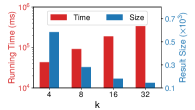
(a) Climate

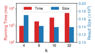
(b) El Nino

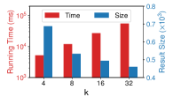
(c) Household

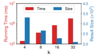
(d) SUSY

Figure 8: Performance of H-GRMR with varying $k$ in the IPDG construction ($\varepsilon=0.1$)

Impact of IPDG Construction: First of all, we test the effect of $k$ in the IPDG construction on the performance of H-GRMR. Figure 8 shows the running time and result sizes of H-GRMR for $k=4,8,16,32$ on four real-world datasets when $\varepsilon$ and $m$ are fixed to $0.1$ and $10^{6}$, respectively. As discussed in Section 4, when $k$ is larger, the running time of H-GRMR increases significantly because the approximate IPDG has more edges, which leads to the increases in both the number of LPs and the number of constraints in each LP for dominance graph construction. Meanwhile, the result sizes of H-GRMR decrease with increasing $k$ because more edges in the exact IPDG are contained in the approximate one and thus the edge weights computed from LPs are tighter and closer to the optimal ones. Nevertheless, the solution quality on El Nino does not improve anymore when $k=16,32$. This is because the approximate IPDG built for $k=8$ has covered almost all edges of the exact IPDG. Using a larger $k$ only leads to more redundant edges in this case. In the remaining experiments, we will use the values of $k$ selected from $[4,8,16,32]$ that can strike the best balance between efficiency and quality of results for H-GRMR. Note that if we fix $k$ and vary $m$ in the IPDG construction, we can observe the same trend as varying $k$: The running time increases while the result sizes decrease for a larger $m$. The results for varying $m$ are omitted due to space limitations.

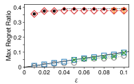
(a) Climate

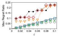
(b) El Nino

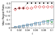
(c) Household

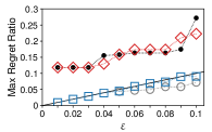
(d) SUSY

Figure 9: Parameter $\varepsilon$ vs. max regret ratio

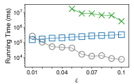
(a) Climate

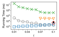
(b) El Nino

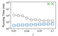
(c) Household

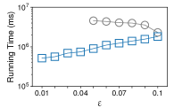
(d) SUSY

Figure 10: Running time with varying $\varepsilon$

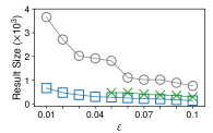
(a) Climate

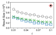
(b) El Nino

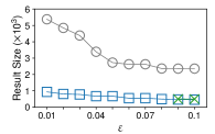
(c) Household

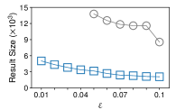
(d) SUSY

Figure 11: Result size with varying $\varepsilon$

Impact of Parameter $\varepsilon$: Next, we vary $\varepsilon$ from $0.01$ to $0.1$ to evaluate the performance of each algorithm. Note that we terminate the execution of an algorithm after running it on a dataset for one day. HD-RRMS and HittingSet suffer from a low efficiency and cannot return any result on a large dataset when $\varepsilon$ is small. In Figure 11, we show the maximum regret ratios of the results of each algorithm for different $\varepsilon$. Similar to the 2D setting, we find empirically that RMS algorithms (Greedy, HD-RRMS, and Sphere) do not provide any valid result for GRMR on real datasets due to the skewness of data distributions. The running time and result sizes of each algorithm with varying $\varepsilon$ are presented in Figures 11 and 11, respectively. First of all, we notice that H-GRMR runs slower when $\varepsilon$ is larger. This is expected, as the dominance graph contains all edges with weights at most $\varepsilon$ and therefore has more edges for a larger $\varepsilon$. It thus takes more time for both graph construction and result computation when $\varepsilon$ is larger. On the other hand, both $\varepsilon$-Kernel and HittingSet run faster when $\varepsilon$ is larger because of smaller sample sizes for computation. In terms of result sizes, all three algorithms identify smaller results with increasing $\varepsilon$, as expected. Finally, compared with $\varepsilon$-Kernel, H-GRMR achieves higher efficiencies in all datasets except Climate. At the same time, H-GRMR produces results of significantly better quality than $\varepsilon$-Kernel: the result size of H-GRMR is up to $5.7$ times smaller than that of $\varepsilon$-Kernel. Compared with HittingSet, H-GRMR runs up to four orders of magnitude faster while providing results with $1.07$–$2.1$ times smaller sizes. In particular, H-GRMR is the only algorithm that returns a valid result for GRMR on SUSY in reasonable time when $\varepsilon<0.05$.

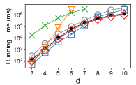
(a) Normal, time

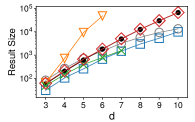
(b) Normal, size

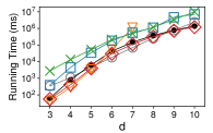
(c) Uniform, time

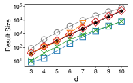
(d) Uniform, size

Figure 12: Performance with varying the dimensionality $d$ ($\varepsilon=0.1$)

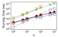
(a) Normal (6D), time

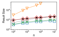
(b) Normal (6D), size

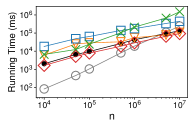
(c) Uniform (6D), time

(d) Uniform (6D), size

Figure 13: Performance with varying the dataset size $n$ ($\varepsilon=0.1$)

Impact of Dimensionality $d$ and Dataset Size $n$: Finally, we evaluate the impact of the dimensionality $d$ and the dataset size $n$ for different algorithms on the two synthetic datasets. In these experiments, we fix $\varepsilon$ to $0.1$. The results for varying dimensionality $d$ ($d=3$ to $10$) are shown in Figure 13. Both the running time and result sizes of all algorithms grow rapidly with $d$. Such results are not surprising, because the number of extreme points in a dataset increases super-linearly with $d$. HD-RRMS and HittingSet are inefficient in high dimensions and cannot return any result on Normal when $d>7$. Greedy and Sphere return valid results for GRMR by solving $2^{d}$ RMS problems. However, their solution quality is clearly inferior to H-GRMR, especially in higher dimensions. Generally, H-GRMR finds results of better quality than any other algorithm in reasonable time when the dimensionality $d$ ranges from $3$ to $10$. The results with varying the dataset size $n$ from $10^{4}$ to $10^{7}$ are illustrated in Figure 13. The trends are generally similar to those for varying $d$. Both the running time and result sizes grow with $n$ because of the increasing number of extreme points. The only exception is that the result size of most algorithms (except $\varepsilon$-Kernel) decreases with $n$ on Uniform. H-GRMR outperforms all other algorithms in terms of quality of results. In particular, the result of H-GRMR is nearly $50$ times smaller than that of $\varepsilon$-Kernel on Uniform when $n=10^{7}$.

6 Related Work

A great variety of approaches to representing a large dataset by a small subset of data points have been proposed recently [1, 28, 7, 49, 6, 12, 40, 4, 39]. One important method that has been extensively investigated is maxima representation [9, 13], which finds a compact subset that contains the maxima (i.e., points with the highest scores) of a dataset for any possible ranking function. According to the class of ranking functions considered, there are many different definitions of maxima representations. In particular, the convex hull [32, 13] and skyline [9] are two examples of maxima representations when the classes of all linear functions and nonnegative monotonic functions are considered, respectively.

In practice, since maxima representations can still be overwhelmingly large [4, 3], recent efforts have been directed toward reducing their sizes using approximation techniques. Nanongkai et al. [28] were the first to propose the regret-minimizing set (RMS) problem for approximate maxima representations. They introduced the regret ratio, which is the relative difference in scores between the top-ranked point of the dataset and the top-ranked point of a subset, as the measure of regret for a ranking function. They used the maximum regret ratio, i.e., the maximum of the regret ratios over all nonnegative (monotonic) linear functions, to measure how well a subset approximates the maxima representation of a dataset. An RMS is defined as the smallest subset whose maximum regret ratio was at most $\varepsilon$. The RMS problem was proven to be NP-hard [10, 2] for any dataset in three or higher dimensions. Since the seminal work of Nanongkai et al., different approximation and heuristic algorithms [28, 31, 3, 2, 24, 41, 34, 10] were proposed for RMS. Please refer to [43] for a survey of algorithmic techniques for RMS.

Furthermore, several works [14, 10, 16, 33, 36, 47, 37, 4, 29, 42, 44] studied different generalizations and variations of RMS. Chester et al. [14] generalized the regret ratio to $k$-regret ratio that expressed the score difference between the top-ranked point in the subset and the $k$^th-ranked point in the dataset. Accordingly, they extended RMS to $k$-RMS for approximating maxima representations of top-$k$ results (instead of top-$1$ results) w.r.t. all ranking functions. Different RMS problems with nonlinear utility functions were studied in [16, 33, 36]. Specifically, they considered convex/concave functions [16], multiplicative functions [33], and submodular functions [36], respectively, but all of which were monotonic. The average regret minimization [47, 37, 34] problem has also been investigated recently. Instead of targeting the maximum regret ratio, it uses the average of regret ratios over all ranking functions as the measure of representativeness. In another variant, Nanongkai el al. [29] and Xie et al. [42] proposed the interactive regret minimization problem by introducing user interactions to enhance RMS. Moreover, Asudeh et al. [4] proposed the ranking-regret representatives (RRR) in which the regret was defined by rankings instead of scores. Specifically, an RRR is the smallest subset that contains at least one of the top-$k$ points in the dataset for all ranking functions. Xie et al. [44] studied a dual problem of RMS called happiness maximization, where the goal is to maximize the happiness (i.e., one minus the regret) instead of minimizing the regret.

Note that all above approaches to approximate maxima representations are designed for monotonic linear (or nonlinear, in some cases) ranking functions. Accordingly, most existing algorithms for RMS and related problems rely on the monotonicity of ranking functions and naturally cannot be directly used for GRMR. To the best of our knowledge, GRMR is the only method that considers the class of all linear functions including non-monotonic ones with negative weights as the ranking functions.

7 Conclusion

In this paper, we proposed the generalized regret-minimizing representative (GRMR) problem to identify the smallest subset that can approximate the maximum score of the dataset for any linear function within a regret ratio of at most $\varepsilon$. We proved the NP-hardness of GRMR in three or higher dimensions. Following a geometric interpretation of GRMR, we designed an exact algorithm for GRMR in two dimension and a heuristic algorithm for GRMR in arbitrary dimensions. Finally, we conducted extensive experiments on real and synthetic datasets to verify the performance of our proposed algorithms. The experimental results confirmed the efficiency, effectiveness, and scalability of our algorithms for GRMR.

Appendix A Proof of Theorem 1

Proof.

For a set $P_{0}$ of $n$ points in $\mathbb{R}^{3}_{+}$ and a positive integer $r\in\mathbb{Z}^{+}$, a 3D RMS instance $\mathsf{RMS}(P_{0},r)$ asks, given a real number $\varepsilon\in(0,1)$, whether there exists a subset $Q_{0}\subseteq P_{0}$ of size $r$ such that $\omega(x,Q_{0})\geq(1-\varepsilon)\cdot\omega(x,P_{0})$ for any $x\in\mathbb{S}^{2}_{+}$. Intuitively, RMS is a restricted version of GRMR where both data points and utility vectors are in the nonnegative orthant. Here, we can restrict $P_{0}\in[0,1]^{3}$ because of the scale-invariance of RMS [28]. We use $l^{+}(Q_{0})=\max_{x\in\mathbb{S}^{2}_{+}}1-\frac{\omega(x,Q_{0})}{\omega(x,P_{0})}$ to denote the maximum regret ratio of $Q_{0}$ over $P_{0}$ for RMS. Given any $\mathsf{RMS}(P_{0},r)$, we should construct an instance $\mathsf{GRMR}(P^{\prime},r^{\prime})$ satisfying that there exists a subset $Q_{0}\subseteq P_{0}$ of size $r$ such that $l^{+}(Q_{0})\leq\varepsilon$ if and only if there exists a subset $Q^{\prime}\subseteq P^{\prime}$ of size $r^{\prime}$ such that $l(Q^{\prime})\leq\varepsilon$ for an arbitrary $\varepsilon\in(0,1)$.

For $\mathsf{RMS}(P_{0},r)$ and $\varepsilon\in(0,1)$, we add three new points $B=\{b_{1},b_{2},b_{3}\}$ to $P_{0}$. Let $b_{1}=(1-\eta,1,1)$, $b_{2}=(1,1-\eta,1)$, and $b_{3}=(1,1,1-\eta)$ where $\eta>3$. The value of $\eta$ should be determined by $P_{0}$, $Q_{0}$, and $\varepsilon$ as discussed later. We will prove that $P_{0}$ has an $\varepsilon$-regret set of size $r$ if and only if $P^{\prime}=P_{0}\cup B$ has an $\varepsilon$-regret set of size $r^{\prime}=r+3$. To prove this, we need to show (1) If $l^{+}(Q_{0})\leq\varepsilon$ and $Q^{\prime}=Q_{0}\cup B$, then $l(Q^{\prime})\leq\varepsilon$; and (2) If $l(Q^{\prime})\leq\varepsilon$, then $B\subset Q^{\prime}$ and, for $Q_{0}=Q^{\prime}\setminus B$, $l^{+}(Q_{0})\leq\varepsilon$ over $P_{0}=P^{\prime}\setminus B$.

We first prove (1) by showing that $l_{x}(Q^{\prime})\leq\varepsilon$ for all $x\in\mathbb{S}^{2}$. First of all, we consider the case when $x\in\mathbb{S}^{2}_{+}$. Let $p^{*}=\arg\max_{p\in P^{\prime}}\langle p,x\rangle$. If $p^{*}\in B$, then $l_{x}(Q^{\prime})=0$ because $B\subset Q^{\prime}$; Otherwise, we have $p^{*}\in P_{0}$ and there always exists some $p\in Q_{0}$ such that $\langle p,x\rangle\geq(1-\varepsilon)\cdot\langle p^{*},x\rangle$ and thus $l_{x}(Q^{\prime})\leq\varepsilon$ because $Q_{0}$ is an $\varepsilon$-regret set of $P_{0}$. Next, we consider the case when $x\in\mathbb{S}^{2}\setminus\mathbb{S}^{2}_{+}$. We want to show that the point with the highest score for any $x\in\mathbb{S}^{2}\setminus\mathbb{S}^{2}_{+}$ is always in $B$ and thus $l_{x}(Q^{\prime})=0$. Furthermore, we consider three cases for $x=(x[1],x[2],x[3])$ as follows:

• Case 1.1 ($x[1]\geq 0,x[2]\geq 0,x[3]\leq 0$): For any $p\in P_{0}$, we have

  $$\langle p,x\rangle\leq p[1]\cdot x[1]+p[2]\cdot x[2]<x[1]+x[2]\leq\sqrt{2}$$

  In addition, we have

  $$\langle b_{3},x\rangle=x[1]+x[2]+(1-\eta)\cdot x[3]\geq\sqrt{2}$$

  Thus, $b_{3}$ always has a larger score than all points in $P_{0}$. This result also holds for $b_{1}$ or $b_{2}$ when $x[1]\leq 0$ or $x[2]\leq 0$ and other dimensions are positive.

• Case 1.2 ($x[1]\geq 0,x[2]\leq 0,x[3]\leq 0$): For any $p\in P_{0}$, $\langle p,x\rangle<x[1]\leq 1$. Moreover, we have

  $$\langle b_{2},x\rangle=x[1]+x[2]+x[3]-\eta\cdot x[2]$$

  and

  $$\langle b_{3},x\rangle=x[1]+x[2]+x[3]-\eta\cdot x[3]$$

  If $x[2]\leq x[3]$, then $\langle b_{2},x\rangle\geq\langle b_{3},x\rangle$, and vice versa. So the minimum of $\max(\langle b_{2},x\rangle,\langle b_{3},x\rangle)$ is always reached when $x[2]=x[3]$. In this case, we have

  $$\langle b_{2},x\rangle=\langle b_{3},x\rangle=x[1]+(2-\eta)\cdot x[2]$$

  Let $x[2]=\beta$ and thus $x[1]=\sqrt{1-2\beta^{2}}$. We consider the score $\langle b_{2},x\rangle$ as a function $f(\beta)$, i.e.,

  $$f(\beta)=\langle b_{2},x\rangle=\sqrt{1-2\beta^{2}}+(2-\eta)\cdot\beta$$

  where $\beta\in[-1,0]$. As $f(\beta)$ first increases and then decreases in the range $[-1,0]$, we have $\langle b_{2},x\rangle\geq f(0)=1$ and $\langle b_{2},x\rangle\geq f(-1)=\eta-2>1$. Thus, the larger one between $\langle b_{2},x\rangle$ and $\langle b_{3},x\rangle$ is always greater than the scores of all points in $P_{0}$ w.r.t. $x$. Similar results can be implied when $x[2]\geq 0$ or $x[3]\geq 0$ and other dimensions are negative.

• Case 1.3 ($x[1]\leq 0,x[2]\leq 0,x[3]\leq 0$): For any $p\in P_{0}$, $\langle p,x\rangle\leq 0$. In addition, there always exists $i\in[1,3]$ such that $x[i]\leq-\frac{\sqrt{3}}{3}$. Taking $x[1]\leq-\frac{\sqrt{3}}{3}$ as an example, we have

  $$\langle b_{1},x\rangle\geq\frac{\sqrt{3}}{3}\cdot\eta-\sqrt{3}>0$$

  because $\eta>3$.

We can prove $l(Q^{\prime})\leq\varepsilon$ from the above three cases.

To verify (2), we need to show: (2.1) If $B\not\subset Q^{\prime}$, then $l(Q^{\prime})>\varepsilon$; (2.2) If $l^{+}(Q_{0})>\varepsilon$, then $Q_{0}\cup B$ is not an $\varepsilon$-regret set of $P^{\prime}$. The correctness of (2.1) is easy to prove: Taking $x=(-1,0,0)\in\mathbb{S}^{2}$, it is obvious that $\langle b_{1},x\rangle>0$ and $\langle p,x\rangle<0$ for any $p\in P^{\prime}\setminus\{b_{1}\}$. So if $B\not\subset Q^{\prime}$, then $l(Q^{\prime})>1$. The proof of (2.2) involves determining the value of $\eta$ according to $P_{0}$, $Q_{0}$, and $\varepsilon$. If $l^{+}(Q_{0})>\varepsilon$, then there exists a point $p\in P_{0}\setminus Q_{0}$ and a vector $x\in\mathbb{S}^{2}_{+}$ such that $(1-\varepsilon)\cdot\langle p,x\rangle>\omega(x,P_{0})$. Since $l^{+}(Q_{0})$ and the vector $x$ with $l^{+}(Q_{0})=l_{x}(Q_{0})$ can be computed by a linear program [28], it is guaranteed that such a point $p$ and a vector $x$ can be found in polynomial time. When $\eta>\frac{3-(1-\varepsilon)\cdot\langle p,x\rangle}{x[i]}$, we have $\langle b_{i},x\rangle<(1-\varepsilon)\cdot\langle p,x\rangle$ ($i=1,2,3$). Therefore, if $l^{+}(Q_{0})>\varepsilon$, $l_{x}(Q^{\prime})>\varepsilon$ once $\eta$ is large enough and thus $Q^{\prime}$ is not an $\varepsilon$-regret set of $P^{\prime}$. We prove (2) from (2.1) and (2.2).

We complete the reduction from RMS in $\mathbb{R}^{3}_{+}$ to GRMR in $\mathbb{R}^{3}$ in polynomial time and hence prove the NP-hardness of GRMR in $\mathbb{R}^{3}$. Since the reduction can be generalized to higher dimensions, GRMR is also NP-hard when $d>3$. ∎

Appendix B Proof of Lemma 1

Proof.

First of all, it is obvious that $R_{\varepsilon}(p)\neq\varnothing$ if $p\in S$ since it must hold that $x^{*}_{i}\in R_{\varepsilon}(p)$. Next, we will prove $R_{\varepsilon}(p)=\varnothing$ if $p\notin S$ by showing the minimum of the regret ratio $l_{x}(p)=1-\frac{\langle p,x\rangle}{\omega(x,P)}$ of $p$ for any $x\in\mathbb{S}^{1}$ is greater than $\varepsilon$. Then, we consider each extreme point $t_{i}\in X$ separately. Let $f(x)=1-\frac{\langle p,x\rangle}{\langle t_{i},x\rangle}$ where $x\in R(t_{i})$ and $t_{i}\in X$. According to Line 1 of Algorithm 1, we have got if $p\notin S$, then $1-\frac{\langle p,x^{*}_{i}\rangle}{\langle t_{i},x^{*}_{i}\rangle}>\varepsilon$ for all $i\in[|X|]$. Thus, we have

$$f(x)=1-\frac{\|p\|}{\|t_{i}\|}\cdot\frac{\cos(\theta(p)-\theta(x))}{\cos(\theta(t_{i})-\theta(x))}$$

where $x\in R(t_{i})$, i.e., $x\in[x^{*}_{i-1},x^{*}_{i}]$. If $\theta(p)<\theta(t)$, $f(x)$ will monotonically increase with increasing $\theta(x)$; If $\theta(p)>\theta(t)$, $f(x)$ will monotonically decrease with increasing $\theta(x)$; And if $\theta(p)=\theta(t)$, $f(x)$ will be a constant $1-\frac{\|p\|}{\|t_{i}\|}$. Thus, the minimum of $f(x)$ can only be reached when $x=x^{*}_{i-1}$ or $x^{*}_{i}$. In addition, we have

$$f(x^{*}_{i-1})=1-\frac{\langle p,x^{*}_{i-1}\rangle}{\langle t_{i-1},x^{*}_{i-1}\rangle}>\varepsilon\quad\textnormal{and}\quad f(x^{*}_{i})=1-\frac{\langle p,x^{*}_{i}\rangle}{\langle t_{i},x^{*}_{i}\rangle}>\varepsilon$$

Combining the above results, we have $l_{x}(p)>\varepsilon$ for any $x\in\mathbb{S}^{1}$ if $\frac{\langle p,x\rangle}{\langle t_{i},x\rangle}<1-\varepsilon$ for any $t_{i}\in X$ and conclude the proof. ∎

Appendix C Proof of Lemma 2

Proof.

Firstly, the removal of any non-extreme point does not lead to any regret and it is safe to only consider extreme points for regret computation. For $s_{i},s_{j}\in S(i<j)$ and $t\in X$ where $\theta(s_{i})\leq\theta(t)\leq\theta(s_{j})$, we need to compute an upper bound $l_{ij}(t)$ of the maximum regret ratio of $\{s_{i},s_{j}\}$ over $t$ for any vector $x\in R(t)$. By sweeping all utility vectors in a counterclockwise direction, we observe that, similar to the proof of Lemma 1,

$$f_{i}(x)=1-\frac{\langle s_{i},x\rangle}{\langle t,x\rangle}=1-\frac{\|s_{i}\|}{\|t\|}\cdot\frac{\cos(\theta(s_{i})-\theta(x))}{\cos(\theta(t)-\theta(x))}$$

monotonically increases with increasing $x$ since $\theta(s_{i})\leq\theta(t)$ while

$$f_{j}(x)=1-\frac{\langle s_{j},x\rangle}{\langle t,x\rangle}=1-\frac{\|s_{j}\|}{\|t\|}\cdot\frac{\cos(\theta(s_{j})-\theta(x))}{\cos(\theta(t)-\theta(x))}$$

monotonically decreases with increasing $x$ since $\theta(s_{j})\geq\theta(t)$. Therefore, the regret ratio of $\{s_{i},s_{j}\}$, i.e., $\min\big{(}f_{i}(x),f_{j}(x)\big{)}$ is maximized when $f_{i}(x)=f_{j}(x)$ (i.e., $\langle s_{i},x\rangle=\langle s_{j},x\rangle$). Finally, we have

$$l_{ij}=\max_{t\in X[s_{i},s_{j}]}1-\frac{\langle s_{i},x\rangle}{\langle t,x\rangle}$$

is the upper bound of the maximum regret ratio of $\{s_{i},s_{j}\}$ after removing the candidates between them. ∎

Appendix D Proof of Lemma 3

Proof.

For each extreme point $t\in X\setminus Q$, there always exists two points $s_{i},s_{j}\in Q$ where $\theta(s_{i})\leq\theta(t)\leq\theta(s_{j})$ and $l_{ij}\leq\varepsilon$ because $C$ is a cycle of $G$. According to Lemma 2, we have the regret ratio of $\{s_{i},s_{j}\}$ over $t$ is at most $\varepsilon$ for any $x\in R(t)$. Moreover, if $t\in X\cap Q$, it is obvious that the maximum regret ratio of $Q$ over $t$ is $0$. Therefore, the maximum regret ratio of $Q$ over $t$ is at most $\varepsilon$ for every $t\in X$ and $Q$ is an $\varepsilon$-regret set of $P$.

A subset $Q\subseteq P$ is called a locally minimal $\varepsilon$-regret set if (1) $Q$ is an $\varepsilon$-regret set and (2) $Q\setminus\{q\}$ is not an $\varepsilon$-regret set for any $q\in Q$. Obviously, the optimal result $Q^{*}_{\varepsilon}$ (i.e., the globally minimum $\varepsilon$-regret set) is guaranteed to be locally minimal. First, if $Q$ is a locally minimal $\varepsilon$-regret set, we can get $Q\subseteq S$. For any $p\notin S$, if a subset $Q^{\prime}$ where $p\in Q^{\prime}$ is an $\varepsilon$-regret set, it will hold that $Q^{\prime}\setminus\{p\}$ is still an $\varepsilon$-regret set since $R_{\varepsilon}(p)=\varnothing$, which implies that $Q^{\prime}$ is not locally minimal. Then, we arrange all points of $Q$ in a counterclockwise direction as $\{q_{1},\ldots,q_{|Q|}\}$. We prove that there exists an edge $(q_{i}\rightarrow q_{i+1})$ in $G$ for every $i\in[|Q|]$ by contradiction. If $(q_{i}\rightarrow q_{i+1})\notin E$, then either (1) $\theta(q_{i+1})-\theta(q_{i})>\pi$ or (2) $1-\frac{\langle q_{i},x^{*}\rangle}{\langle t,x^{*}\rangle}>\varepsilon$ when $\langle q_{i},x^{*}\rangle=\langle q_{i+1},x^{*}\rangle$. In the previous case, we have $l(Q)>1$ and $Q$ is not an $\varepsilon$-regret set. In the latter case, if there does not exist any $i^{\prime}<i$ or $i^{\prime\prime}>i+1$ such that the regret ratio of $\{q_{i},q_{i+1}\}\cup\{q_{i^{\prime}}\}$ or $\{q_{i},q_{i+1}\}\cup\{q_{i^{\prime\prime}}\}$ for $x^{*}$ is at most $\varepsilon$, we will have $l_{x^{*}}(Q)>\varepsilon$ and $Q$ is not an $\varepsilon$-regret set; Otherwise, if there exists such $i^{\prime}<i$ or $i^{\prime\prime}>i+1$, we will have $q_{i}$ or $q_{i+1}$ is redundant and $Q$ is not locally minimal. Based on all above results, we conclude that there exists a cycle $C$ of $G$ corresponding to $Q$ as long as $Q$ is a locally minimal $\varepsilon$-regret set of $P$. ∎

References

- Agarwal et al. [2004] P. K. Agarwal, S. Har-Peled, and K. R. Varadarajan. Approximating extent measures of points. J. ACM, 51(4):606–635, 2004.
- Agarwal et al. [2017] P. K. Agarwal, N. Kumar, S. Sintos, and S. Suri. Efficient algorithms for k-regret minimizing sets. In SEA, pages 7:1–7:23, 2017.
- Asudeh et al. [2017] A. Asudeh, A. Nazi, N. Zhang, and G. Das. Efficient computation of regret-ratio minimizing set: A compact maxima representative. In SIGMOD, pages 821–834, 2017.
- Asudeh et al. [2019] A. Asudeh, A. Nazi, N. Zhang, G. Das, and H. V. Jagadish. RRR: rank-regret representative. In SIGMOD, pages 263–280, 2019.
- Aurenhammer [1991] F. Aurenhammer. Voronoi diagrams - A survey of a fundamental geometric data structure. ACM Comput. Surv., 23(3):345–405, 1991.
- Bachem et al. [2018] O. Bachem, M. Lucic, and A. Krause. Scalable k-means clustering via lightweight coresets. In KDD, pages 1119–1127, 2018.
- Badanidiyuru et al. [2014] A. Badanidiyuru, B. Mirzasoleiman, A. Karbasi, and A. Krause. Streaming submodular maximization: massive data summarization on the fly. In KDD, pages 671–680, 2014.
- Barber et al. [1996] C. B. Barber, D. P. Dobkin, and H. Huhdanpaa. The quickhull algorithm for convex hulls. ACM Trans. Math. Softw., 22(4):469–483, 1996.
- Börzsönyi et al. [2001] S. Börzsönyi, D. Kossmann, and K. Stocker. The skyline operator. In ICDE, pages 421–430, 2001.
- Cao et al. [2017] W. Cao, J. Li, H. Wang, K. Wang, R. Wang, R. C. Wong, and W. Zhan. k-regret minimizing set: Efficient algorithms and hardness. In ICDT, pages 11:1–11:19, 2017.
- Casals and Martinez [2013] M. Casals and A. J. Martinez. Modeling player performance in basketball through mixed models. International Journal of Performance Analysis in Sport, 13(1):64–82, 2013.
- Celis et al. [2018] L. E. Celis, V. Keswani, D. Straszak, A. Deshpande, T. Kathuria, and N. K. Vishnoi. Fair and diverse dpp-based data summarization. In ICML, pages 715–724, 2018.
- Chang et al. [2000] Y. Chang, L. D. Bergman, V. Castelli, C. Li, M. Lo, and J. R. Smith. The onion technique: Indexing for linear optimization queries. In SIGMOD, pages 391–402, 2000.
- Chester et al. [2014] S. Chester, A. Thomo, S. Venkatesh, and S. Whitesides. Computing k-regret minimizing sets. PVLDB, 7(5):389–400, 2014.
- Dijkstra [1959] E. W. Dijkstra. A note on two problems in connexion with graphs. Numerische Mathematik, 1:269–271, 1959.
- Faulkner et al. [2015] T. K. Faulkner, W. Brackenbury, and A. Lall. k-regret queries with nonlinear utilities. PVLDB, 8(13):2098–2109, 2015.
- Fowler et al. [1981] R. J. Fowler, M. Paterson, and S. L. Tanimoto. Optimal packing and covering in the plane are np-complete. Inf. Process. Lett., 12(3):133–137, 1981.
- Fredman and Tarjan [1987] M. L. Fredman and R. E. Tarjan. Fibonacci heaps and their uses in improved network optimization algorithms. J. ACM, 34(3):596–615, 1987.
- Graham [1972] R. L. Graham. An efficient algorithm for determining the convex hull of a finite planar set. Inf. Process. Lett., 1(4):132–133, 1972.
- Har-Peled [2011] S. Har-Peled. On the expected complexity of random convex hulls. CoRR, abs/1111.5340, 2011.
- Ilyas et al. [2008] I. F. Ilyas, G. Beskales, and M. A. Soliman. A survey of top-k query processing techniques in relational database systems. ACM Comput. Surv., 40(4):11:1–11:58, 2008.
- Inaba et al. [1994] M. Inaba, N. Katoh, and H. Imai. Applications of weighted Voronoi diagrams and randomization to variance-based k-clustering. In SoCG, pages 332–339, 1994.
- Kalyvas and Tzouramanis [2017] C. Kalyvas and T. Tzouramanis. A survey of skyline query processing. CoRR, abs/1704.01788, 2017.
- Kumar and Sintos [2018] N. Kumar and S. Sintos. Faster approximation algorithm for the k-regret minimizing set and related problems. In ALENEX, pages 62–74, 2018.
- Luo et al. [2009] G. Luo, K. Wu, and P. S. Yu. Answering linear optimization queries with an approximate stream index. Knowl. Inf. Syst., 20(1):95–121, 2009.
- Malkov and Yashunin [2020] Y. A. Malkov and D. A. Yashunin. Efficient and robust approximate nearest neighbor search using hierarchical navigable small world graphs. IEEE Trans. Pattern Anal. Mach. Intell., 42(4):824–836, 2020.
- Morozov and Babenko [2018] S. Morozov and A. Babenko. Non-metric similarity graphs for maximum inner product search. In NeurIPS, pages 4726–4735, 2018.
- Nanongkai et al. [2010] D. Nanongkai, A. D. Sarma, A. Lall, R. J. Lipton, and J. J. Xu. Regret-minimizing representative databases. PVLDB, 3(1):1114–1124, 2010.
- Nanongkai et al. [2012] D. Nanongkai, A. Lall, A. D. Sarma, and K. Makino. Interactive regret minimization. In SIGMOD, pages 109–120, 2012.
- Orlin and Sedeño-Noda [2017] J. B. Orlin and A. Sedeño-Noda. An O(nm) time algorithm for finding the min length directed cycle in a graph. In SODA, pages 1866–1879, 2017.
- Peng and Wong [2014] P. Peng and R. C. Wong. Geometry approach for k-regret query. In ICDE, pages 772–783, 2014.
- Preparata and Shamos [1985] F. P. Preparata and M. I. Shamos. Computational Geometry - An Introduction. Springer, 1985.
- Qi et al. [2018] J. Qi, F. Zuo, H. Samet, and J. C. Yao. K-regret queries using multiplicative utility functions. ACM Trans. Database Syst., 43(2):10:1–10:41, 2018.
- Shetiya et al. [2019] S. Shetiya, A. Asudeh, S. Ahmed, and G. Das. A unified optimization algorithm for solving “regret-minimizing representative” problems. PVLDB, 13(3):239–251, 2019.
- Shewchuk [2002] J. R. Shewchuk. Delaunay refinement algorithms for triangular mesh generation. Comput. Geom., 22(1-3):21–74, 2002.
- Soma and Yoshida [2017] T. Soma and Y. Yoshida. Regret ratio minimization in multi-objective submodular function maximization. In AAAI, pages 905–911, 2017.
- Storandt and Funke [2019] S. Storandt and S. Funke. Algorithms for average regret minimization. In AAAI, pages 1600–1607, 2019.
- Tan et al. [2019] S. Tan, Z. Zhou, Z. Xu, and P. Li. On efficient retrieval of top similarity vectors. In EMNLP/IJCNLP (1), pages 5235–5245, 2019.
- Wang et al. [2019a] Y. Wang, Y. Li, and K. Tan. Coresets for minimum enclosing balls over sliding windows. In KDD, pages 314–323, 2019a.
- Wang et al. [2019b] Y. Wang, Y. Li, and K. Tan. Efficient representative subset selection over sliding windows. IEEE Trans. Knowl. Data Eng., 31(7):1327–1340, 2019b.
- Xie et al. [2018] M. Xie, R. C. Wong, J. Li, C. Long, and A. Lall. Efficient k-regret query algorithm with restriction-free bound for any dimensionality. In SIGMOD, pages 959–974, 2018.
- Xie et al. [2019] M. Xie, R. C. Wong, and A. Lall. Strongly truthful interactive regret minimization. In SIGMOD, pages 281–298, 2019.
- Xie et al. [2020a] M. Xie, R. C. Wong, and A. Lall. An experimental survey of regret minimization query and variants: bridging the best worlds between top-k query and skyline query. VLDB J., 29(1):147–175, 2020a.
- Xie et al. [2020b] M. Xie, R. C. Wong, P. Peng, and V. J. Tsotras. Being happy with the least: Achieving -happiness with minimum number of tuples. In ICDE, pages 1009–1020, 2020b.
- Xin et al. [2007] D. Xin, J. Han, and K. C. Chang. Progressive and selective merge: computing top-k with ad-hoc ranking functions. In SIGMOD, pages 103–114, 2007.
- Yu et al. [2012] A. Yu, P. K. Agarwal, and J. Yang. Processing a large number of continuous preference top-k queries. In SIGMOD, pages 397–408, 2012.
- Zeighami and Wong [2019] S. Zeighami and R. C. Wong. Finding average regret ratio minimizing set in database. In ICDE, pages 1722–1725, 2019.
- Zhou et al. [2019] Z. Zhou, S. Tan, Z. Xu, and P. Li. Möbius transformation for fast inner product search on graph. In NeurIPS, pages 8216–8227, 2019.
- Zhuang et al. [2016] H. Zhuang, R. Rahman, X. Hu, T. Guo, P. Hui, and K. Aberer. Data summarization with social contexts. In CIKM, pages 397–406, 2016.