Detecting Exoplanets Using Eclipsing Binaries as Natural Starshades

Abstract

We investigate directly imaging exoplanets around eclipsing binaries, using the eclipse as a natural tool for dimming the binary and thus increasing the planet to star brightness contrast. At eclipse, the binary becomes point-like, making coronagraphy possible. We select binaries where the planet-star contrast would be boosted by $>10\times$ during eclipse, making it possible to detect a planet that is $\gtrsim 10\times$ fainter or in a star system that is $\sim 2$-$3\times$ more massive than otherwise. Our approach will yield insights into planet occurrence rates around binaries versus individual stars. We consider both self-luminous (SL) and reflected light (RL) planets. In the SL case, we select binaries whose age is young enough so that an orbiting SL planet would remain luminous; in U Cep and AC Sct, respectively, our method is sensitive to SL planets of $\sim$4.5$M_{J}$ and $\sim$9$M_{J}$ with current ground- or near-future space-based instruments, and $\sim$1.5$M_{J}$ and $\sim$6$M_{J}$ with future ground-based observatories. In the RL case, there are three nearby ($\lesssim 50$ pc) systems—V1412 Aql, RR Cae, RT Pic—around which a Jupiter-like planet at a planet-star separation of $\gtrsim 20$ mas might be imaged with future ground- and space-based coronagraphs. A Venus-like planet at the same distance might be detectable around RR Cae and RT Pic. A habitable Earth-like planet represents a challenge; while the planet-star contrast at eclipse and planet flux are accessible with a 6-8m space telescope, the planet-star separation is 1/3 - 1/4 of the angular separation limit of modern coronagraphy.

1 Introduction

Coronagraphs, nulling interferometry, and man-made starshades are the existing strategies for imaging exoplanets directly. Is there a way to dramatically improve these techniques? Here we consider using the eclipse in an eclipsing binary system to dim the observed brightness of the primary and increase the planet to star flux contrast, i.e., we explore the possibility of employing a natural starshade as a tool to find additional exoplanets around binaries via direct imaging, along with the mentioned techniques.

The NASA Exoplanet Archive (Akeson et al., 2013) lists 270 binary systems with exoplanets, but only six binaries have planets detected via direct imaging (Burgasser et al., 2010; Kuzuhara et al., 2011; Currie et al., 2014; Kraus et al., 2014; Gauza et al., 2015; Janson et al., 2019). All six are self-luminous planets with minimum masses intermediate between 6 and 20 $M_{J}$. Our alternate direct imaging method can explore a new parameter space by 1) targeting binaries or stars that are unusual compared to previously observed exoplanet systems and 2) making different (fainter) types of planets accessible.

Planets in binary systems could represent an important fraction of planet demography, especially given that $\sim 45\%$ of Sun-like stars in the Galactic field are part of a multiple system (Raghavan et al., 2010). Parker & Quanz (2013) estimate statistically the percentage of Solar System analogues, defined either as an individual G dwarf or a binary system with separation $>100$-300 AU and a G dwarf component, that host exoplanets. This percentage declines from 65-95% to 20-65% from 1 to 100 AU for planets on circumprimary (S-type) orbits, whereas it increases from 5-59% to 34-75% from 1 to 100 AU for planets on circumbinary (P-type) orbits.

The effect of binarity, relative to single stars, on planet occurrence rates is uncertain. On one hand, the proximity of a stellar companion could induce disk truncation (Jang-Condell, 2015) and suppress planet formation (Moe & Kratter, 2019), reducing (by $0.3\times$) the occurrence rate compared to that in wider binary or individual star systems (Kraus et al., 2016). On the other hand, Matson et al. (2018) do not observe this suppression within $\simeq 50$ AU, and some planets have been discovered orbiting in S-type configurations within tight binary systems (e.g., Thebault & Haghighipour, 2015). Furthermore, the material-rich environments that form massive stars and binaries may readily produce high-mass protoplanetary disks and then gas giant planets (Kennedy & Kenyon, 2008).

Zorotovic & Schreiber (2013) analyze detached post-common-envelope binaries and find that 90% of those observed for $\sim$5 years have eclipse timing variations that could be explained by a circumbinary companion. The Search for Planets Orbiting Two Stars (SPOTS) survey (Thalmann et al., 2014; Bonavita et al., 2016; Asensio-Torres et al., 2018) constrains the frequency of wide ($<$ 1000 AU) orbit substellar companions to between 0.9% and 9%, consistent with that around single stars. The combination of the low rate from the SPOTS survey and the high frequency from the Zorotovic & Schreiber (2013) study suggests a second generation scenario of planet formation around post-common-envelope binaries, i.e., the planet forms after the binary. In this context, our approach has the potential not only to yield further insights on planet occurrence rates around binaries, but also to differentiate among theories of planet formation in binary environments.

Using eclipsing binaries to image exoplanets directly could also expand our knowledge of the kinds of binaries around which planets can form and evolve. For example, while planets have been discovered around eclipsing binaries using the eclipse timing method (HW Vir, Lee et al. 2009; DP Leo, Qian et al. 2010; NN Ser, Qian et al. 2009; Beuermann et al. 2010; NY Vir, Qian et al. 2012a; RR Cae, Qian et al. 2012b), the host properties are narrow and biased. The hosts are generally short-period compact binaries with a low-mass star or a white dwarf component, as the eclipse minimum can be timed more precisely in these cases. Instead, for our method to work efficiently, we require that the dip in magnitude at eclipse is large enough to yield a substantial gain in contrast, regardless of the type of components.

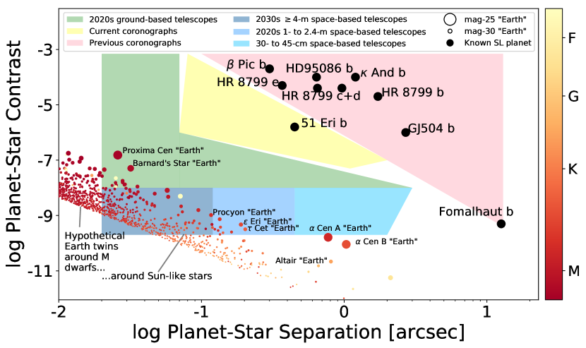
Figure 1: Planet-to-star contrast versus separation plane for the direct imaging method. The capabilities of existing or planned instruments are bundled into different technology zones (colored regions): in pink, VLT-NACO (Lenzen et al., 2003; Rousset et al., 2003), Subaru-HiCIAO (Tamura et al., 2006), Keck-NIRC2 (McLean & Chaffee, 2000); in yellow, VLT-SPHERE (Beuzit et al., 2008), Gemini-GPI (Macintosh et al., 2014), JWST-NIRCam (Krist et al., 2007); in green, EELT-EPIC (Kasper et al., 2008), TMT-PSI (Guyon et al., 2018), TMT-PFI and SEIT (Crossfield, 2013); in blue, WFIRST-CGI (Bailey et al., 2018), LUVOIR-ECLIPS (Juanola-Parramon et al., 2019) and HabEx (Gaudi et al., 2020). The gap between 30- to 45-cm space based telescopes (lightest blue) and previous coronagraphs (pink) is not significant. The groups of instruments defining each colored technology zone vary in their wavelength coverage, so our comparisons to them are rough guides to what is possible. Here, we plot self-luminous planets already discovered through direct imaging with infrared coronagraphs (black points) as well as simulated “Earths” that could be directly imaged in reflected light (colored points). The “Earths” are assumed to lie around a sample of M–F type stars within 20 pc; their color encodes the spectral type of the host, while their size is scaled according to the apparent infrared magnitude of the planet. Not surprisingly, no “Earths” falls within the reach of existing instruments (yellow).

Here we present the application of the natural-starshade method to both self-luminous (SL) and reflected light (RL) planets, in order to assess whether eclipsing binaries represent competitive targets for potential detections with current or future imaging technology. Figure 1 illustrates the observational space and depicts previous, current, and future imaging facilities according to their actual or expected performances. Some directly imaged self-luminous exoplanets are shown in Figure 1 for comparison: $\beta$ Pic b (Lagrange et al., 2009, 2010), HD 95086 b (Rameau et al., 2013), $\kappa$ And b (Carson et al., 2013), HR 8799 b,c,d,e (Marois et al., 2008, 2010), 51 Eri b (Macintosh et al., 2015), GJ 504 b (Kuzuhara et al., 2013), and Fomalhaut b (Kalas et al., 2008), which could be surrounded by a cloud of dust or a disk (Galicher et al., 2013; Lawler et al., 2015), or due to a massive collision of two planetesimals (Gaspar & Rieke, 2020).

We also simulate the presence of an Earth-twin (i.e., same radius and albedo as Earth, and flux received from the binary equal to the solar constant) around a sample of nearby (within 20 pc) stars ranging from M to F type. No datapoint falls in the current technology zone, meaning that the detection of an Earth-like planet around these stars, by means of direct imaging of the reflected light, is not yet feasible. One problem is that an Earth sibling around most M dwarfs would be located at a planet to star separation well below the inner working angle (IWA) of current coronagraphic instruments, i.e., below the detectable angular separation limit. Another issue is that the combination of stellar luminosity and simulated Earth luminosity places these planets below achievable planet to star contrast levels.

Targeting an eclipsing binary has an advantage over a regular binary due to the increased planet to star contrast at the moment of eclipse. This is particularly relevant for planets observable in reflected light, as their brightness would arise from both stars, while the observed starlight would be only from the fainter component of the system. In other words, the eclipse-induced luminosity dip affects only the observed luminosity of the binary system, whereas the reflected luminosity of the planet remains unaltered.

This paper is structured so that we present a catalog of eclipsing binaries, along with the photometric, astrometric, and spectroscopic properties compiled for this study, in Section 2. We consider the detectability of both self-luminous planets and of reflected light Jupiter-, Venus-, and Earth-like planets in Sections 3 and 4, respectively. We then describe the advantages of our approach with respect to single stars and binary systems that do not eclipse in Section 5 and report our conclusions in Section 6.

2 Eclipsing Binary Sample

We compile a list of eclipsing binary systems from the Catalog of Algol Type Binary Stars (Budding et al., 2004) and the Catalog of Eclipsing Variables (Malkov et al., 2006). To determine the best targets for directly imaging exoplanets during eclipse, we consider those binaries for which the depth of the primary minimum (Dmag) is larger than 2.5, i.e., for which the luminosity dimming factor is at least 10. Overall, 289 eclipsing binary systems satisfy the Dmag constraint: 58 from the first catalog and 231 from the second (also considering the latter’s updated version in Avvakumova et al. 2013). In Table A in Appendix A, we list all these eclipsing binary systems, along with the photometric, astrometric, and spectroscopic properties relevant for our work here. If these two catalogs report significantly different values of Dmag in the same photometric filter, we exclude that binary from our subsequent analysis, but report it for completeness in Table A.

The Dmag $>2.5$ criterion selects mostly classical Algols, i.e., with an evolutionary class of SA (Avvakumova et al., 2013). These binaries have a B- or A-type main sequence accretor and a G- or K-type subgiant or giant donor that is large enough to completely eclipse the primary. Observationally, classical Algols are characterized by a deep primary eclipse, shallow secondary eclipse, and ellipsoidal modulations between eclipses due the giant filling its Roche lobe and having a distorted (non-spherical) shape (Budding et al., 2004; Moe & Di Stefano, 2015).

2.1 Distances

Distance is a key factor in limiting direct planet imaging. Because distance data in both catalogs are incomplete, we retrieve parallaxes from the Gaia Second Data Release (DR2) (Gaia Collaboration, 2016, 2018). As explained in Gaia Collaboration (2018), the parallaxes might be associated with either the photocenter of the system or one of the two components, because all Gaia DR2 targets were treated as individual sources.

To check that these DR2 parallaxes are generally consistent with previous measurements, we compare them with Gaia DR1 or Hipparcos measurements (Figure 2). The RMS of the residuals with respect to the 1-to-1 line is 0.81 mas, roughly consistent with the mean of the plotted DR1 and Hipparcos measurement errors (0.5 mas) and about $10\times$ larger than the mean of the DR2 errors (0.05 mas). There is a slight and expected increase in the scatter at small parallaxes, but, overall, the two datasets are consistent within the published measurement uncertainties. There are no large systematics.

For binary systems characterized by an orbital period longer than 2 yr, there might be a mismatch between the parallaxes or proper motions listed in Gaia DR2 with respect to the Tycho-Gaia astrometric solution (TGAS) subset of Gaia DR1 (Lindegren et al., 2016). In our case, the CI Cyg, AR PAV, V381 Sco, and V1329 Cyg systems have periods exceeding this threshold. Considering this and their large distances, we exclude them from our subsequent analysis.

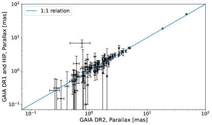
Figure 2: Comparison of parallaxes reported in Gaia DR2 (and used in our analysis; Table A) with those in Gaia DR1 or Hipparcos, where available. The two datasets are consistent to within the published measurement uncertainties and do not show any large systematics.

2.2 Luminosities

Along with astrometry, Gaia DR2 provides stellar luminosities (Andrae et al., 2018). The luminosities are inferred via the FLAME module, which is part of the Apsis data processing pipeline (Bailer-Jones et al., 2013). As the authors specify, there are two potential sources of systematic errors: the adopted bolometric correction BC${}_{\text{G},\odot}$ and extinction. The former is estimated to be +0.06 mag. The latter is assumed to be zero when calculating the absolute magnitude, therefore resulting in underestimated luminosity values (Andrae et al., 2018).

As we did for the distances in the previous section, we test for consistency of the luminosities with previous measurements (Figure 3). The comparison is performed between DR2 luminosities and those inferred from B and V magnitudes from the literature in SIMBAD. Most of the SIMBAD values belong to the Tycho-2 catalog of the 2.5 million brightest stars (Høg et al., 2000), whereas other entries are taken from the Fourth US Naval Observatory CCD Astrograph Catalog (Zacharias et al., 2013) and the fourth RAVE Data Release (Munari et al., 2014).

Both the B and V magnitudes are used to determine the bolometric correction with the following empirical calibration obtained from the catalog of nearby ($<8$ pc) stars (Reid et al., 1995):

$$\text{BC}=\begin{cases}(B-V)<1.2:\\ \ \ -0.121112+0.634846(B-V)-1.01318(B-V)^{2}+\\ \ \ 0.125024(B-V)^{3};\\ (B-V)>1.0:\\ \ \ -43.9614+115.958(B-V)-110.511(B-V)^{2}+\\ \ \ 44.7847(B-V)^{3}-6.74903(B-V)^{4}.\end{cases}$$ (1)

The V magnitude is converted from apparent to absolute scale using the distances retrieved from Gaia DR2. We then convert the absolute magnitude ($M_{V}$) into bolometric luminosity with

$$\text{L}_{\text{bol}}=2.512^{-(M_{V}-4.83)+(\text{BC}-\text{BC}_{\odot})},$$ (2)

where BC${}_{\odot}=-0.076$.

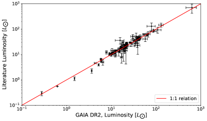
Figure 3: Comparison of bolometric luminosities reported in Gaia DR2, and listed in Table A, with those inferred from B and V magnitudes in SIMBAD. The two datasets are consistent within the measurement uncertainties, and there is no evident sign of systematics.

Considering Figure 3, the RMS of the residuals with respect to the 1-to-1 line is 10.4 L_⊙, which is roughly consistent with the mean of the plotted SIMBAD (Wenger et al., 2000) measurement errors (7.3 L_⊙) and $>2$ times larger than that of the Gaia DR2 errors (4.1 L_⊙). There are no obvious systematics. An additional source of uncertainty in the luminosity would arise if the measurements were made during the eclipse. However, the consistency of the two datasets here suggests that this possibility is unlikely.

3 Detecting Self-Luminous Planets

To quantify the advantage of using an eclipsing binary to directly image an orbiting SL planet requires that we estimate the binary’s age and assume that the binary and SL planet formed at the same time. We can then model the fading of the SL planet as it cools (e.g. Marley et al., 2007; Mordasini, 2013; Mordasini et al., 2017) and ask if it is currently bright enough to be detected (Fortney et al., 2010) by existing or near-future instruments. In the following discussion, we constrain the ages of our binaries using Algol models (van Rensbergen et al., 2010; Mennekens & Vanbeveren, 2017) in Section 3.1. Some with large total masses are likely young enough to host detectable SL planets. We then select two with the youngest age ranges as potential targets for SL planet direct imaging follow-up in Section 3.2.

3.1 Ages

Neither the eclipsing binary catalogs from which we construct our sample nor the Gaia DR2 report ages, which are expected with the third release of Gaia. Determining the ages of our binaries is challenging regardless; as discussed earlier, our Dmag $>2.5$ criterion tends to select classical Algols. Late B-dwarf classical Algols are field blue stragglers, and, because they are rejuvenated by the mass transfer, are older than would be expected from the main sequence lifetime of the current primary (Paczyński, 1971; Giannuzzi, 1984; Iben & Tutukov, 1987). The total mass of the binary system is a better proxy for age.

Mass transfer is nearly conservative for binaries with initially A- or late-B type primaries that interact via Case A Roche-lobe overflow (van Rensbergen et al., 2010; Mennekens & Vanbeveren, 2017). Under these circumstances, the total mass of the current system ($M_{\text{tot}}$) is assumed equal to the sum of the components’ masses when they reached the zero-age main sequence. Then, the initial mass of the primary is

$$M_{\text{primary}}=\frac{M_{\text{tot}}}{q+1},$$ (3)

where $q$ is the initial mass ratio. If the components are initially the same, $q=1$ and the minimum $M_{\text{primary}}$ is $0.5M_{\text{tot}}$. For stable mass transfer to occur with a late-B primary, $q\geq 0.4$ and the maximum $M_{\text{primary}}$ is $0.7M_{\text{tot}}$. Given that the initial primary has now evolved into a subgiant or giant, and that the time it spent on the main sequence was much longer, its main sequence lifetime provides an estimate of the binary’s age. Assuming $0.5M_{\text{tot}}\leq M_{\text{\text{primary}}}\leq 0.7M_{\text{tot}}$, with $M_{\text{tot}}$ obtained from the component masses in Budding et al. (2004), and the relationship between stellar mass and main sequence lifetime, we convert this $M_{\text{primary}}$ range into an age range for each of our binaries. This range could extend to younger ages if mass loss affects the transfer process ($M_{\text{primary}}>0.7M_{\text{tot}}$), but we proceed with the conservative (older) age estimates above.

Table 1: Best Eclipsing Binary Targets for Direct Detection of Self-Luminous Exoplanets

Name	$m_{V}$	DmagV	$m_{J}$	DmagJ	d	Period	$t_{\text{Dmag}}$	$a_{\text{bin}}$	$M_{1}$	$M_{2}$	Spec Type	Age Interval
					[pc]	[days]	[min]	[AU]	[M⊙]	[M⊙]		[Myr]
U Cep	6.9	2.54	6.47	1.10	198.6	2.5	90	0.07	4.20	2.30	B7V+[G8III-IV]	215-525
AC Sct	10.0	2.60	9.72	1.62	985.6	4.8	168	0.11	2.80	1.40	B9+[G0IV]	640-1365

At present, there are few detections of SL planets around binaries with massive stars. Observational studies such as the on-going BEAST survey (Janson et al., 2019) aim to address the question of exoplanets around B-type stars. Our binaries have the potential to shed more light on whether the incidence of massive planets increases or declines with host stellar mass, thus constraining the stellar mass interval within which planet formation is favorable (Janson et al., 2011, 2019).

3.2 Best targets

We shortlist the best eclipsing binaries for observational follow-up according to the criteria discussed previously: 1) depth of primary eclipse larger than 2.5 mag, 2) accessibility with current or near-future technology, and 3) likelihood that the binary is young, and thus that any orbiting SL planet is luminous, based on the binary total mass. The two youngest eclipsing binaries satisfying these criteria are U Cep and AC Sct, with age intervals of 215-525 Myr and 640-1365 Myr, respectively (Table 1).

An additional consideration for selecting suitable targets is whether the binary system has a tertiary companion. Tokovinin et al. (2006) show that short period ($P$) binaries are more likely to have a third component which, if orbiting at small separation, could suppress planet formation (Moe & Kratter, 2019). In particular, no circumbinary planet has been found around a $P<7$ days binary, which may be due to the presence of a tertiary (Hamers et al., 2016). In our case, U Cep ($P=2.5$ days) is known to have a third companion (Tokovinin, 2018) at $\sim$2800 AU, so its influence on a potential planet’s dynamical stability is negligible. It is not known whether AC Sct ($P=4.8$ days) has a tertiary component.

The projected separation between the binary stellar components is 0.07 AU for U Cep and 0.11 AU for AC Sct (Brancewicz, & Dworak, 1980). Therefore, we would expect any potential planet to lie on a P-type orbit. Because the eccentricities of the systems are not available, we cannot assess the long-term stability of the planetary orbits (Holman & Wiegert, 1999; Quarles, & Lissauer, 2016) at this time.

We add two more potential targets, V621 Cen and RW Mon, if we relax our deep eclipse criterion from Dmag $>2.5$ to $>2.0$ mag, a contrast improvement of $\sim$6$\times$. The total mass of V621 Cen corresponds to an age range of 196-478 Myr, i.e., comparable to U Cep’s, but detecting SL planets around V621 Cen would require future planned facilities due to its large distance (1.8 kpc). RW Mon is closer (505 pc) and has an age range of 880-2150 Myr. RW Mon’s period variations may arise from a close tertiary companion (Soydugan et al., 2011), so targeting this system would not only test our direct imaging method, but also reveal the nature of any third component. There could be other good targets within our sample, but some binaries have missing or conflicting data, e.g., Dmag, which prevents us from evaluating them.

For U Cep and AC Sct, we calculate whether the eclipse would increase the infrared SL planet-star contrast to that required by the instruments. We consider planet masses between 0.5 and $10M_{J}$, determining the corresponding planet $J$-band (1.25 $\mu m$) magnitude at the age of the binaries with the Sonora evolutionary models (Marley et al. 2020, in prep.). We then estimate the planet-star contrast at eclipse and compare it with the technology regions as in Figure 1.

The planet-star contrast during the eclipse is the ratio of the planet luminosity to the primary minimum. The eclipsing binary catalogs report the Dmag value for U Cep and AC Sct in the $V$-band. Thus, we estimate Dmag in $J$-band based on the $V-J$ color of both binary components. Formally, we write the fluxes normalized to the total flux in the $V$-band, i.e., $F_{\text{p},V}+F_{\text{s},V}=1$, where $F_{\text{p},V}$ and $F_{\text{s},V}=10^{-0.4\text{Dmag}_{V}}$ are the primary and secondary $V$-band fluxes, respectively. Then, we have

$$\text{Dmag}_{J}=-2.5\log\left(\frac{F_{\text{s},J}}{F_{\text{tot},J}}\right)$$ (4)

where $F_{\text{s},J}=F_{\text{s},V}10^{0.4(V-J)_{\text{s}}}$ and $F_{\text{tot},J}=F_{\text{p},J}+F_{\text{s},J}$, where $F_{\text{p},J}=F_{\text{p},V}10^{0.4(V-J)_{\text{p}}}$.

The $J$-band luminosity during the eclipse is then calculated as

$$\text{L}_{J,e}=10^{-0.4\text{Dmag}_{J}}\text{L}_{J}$$ (5)

where L_J and L_J,e are the $J$-band luminosities at maximum brightness and primary minimum, respectively.

Figure 4 illustrates the planet-star contrast versus separation plane for U Cep and AC Sct. Around U Cep, planets of $\gtrsim 4.5M_{J}$ reach contrast levels $\gtrsim 10^{-7}$ and are thus detectable with current ground- or near-future space-based instruments. Planets of 3-4$M_{J}$ and roughly 1.5-2.5$M_{J}$ achieve contrast levels associated with future ground- ($\sim$10^-8) and space-based ($\sim$10^-9) facilities, respectively. Around AC Sct, $\gtrsim$9$M_{J}$ planets can be detected with current ground- or near-future space-based instruments, while 6-8$M_{J}$ and 3-5$M_{J}$ planets require future ground- and space-based observatories, respectively.

In Figure 4, the technology regions are the same as in Figure 1 and defined by the instrument performance and inner-working angle. The location of the simulated planets on the planet-star separation axis is arbitrary. Current ground- or near-future space-based instruments are characterized by observable separations of roughly 0.1-2 arcsec. At the distances of U Cep and AC Sct, this range translates into orbital semi-major axes of 20-400 AU and 100-2000 AU, respectively, consistent with those of known directly imaged planets around binaries (Schwarz et al., 2016).

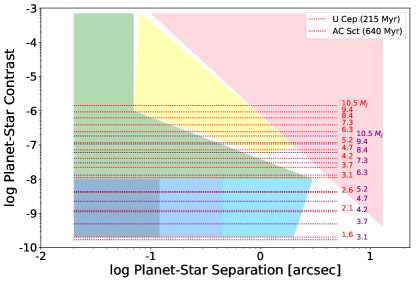
Figure 4: Planet-star $J$-band contrast versus separation for simulated SL planets around U Cep (red) and AC Sct (purple). The planet-star contrast is the ratio of the planet to binary luminosity at eclipse. The numerator is derived from the Sonora evolutionary models (Marley et al. 2020, in prep.), assuming that the planet is as old as the estimated binary age. The denominator is equivalent to the $J$-band Dmag, which is estimated from the $V-J$ colors of the binary components (see Eq. 4). Current and future observational facilities are denoted by the colored regions as in Figure 1. Around U Cep, current ground- or near-future space-based (yellow), future ground-based (green), and future space-based (blue) instruments can detect $\gtrsim 5M_{J}$, 3-4$M_{J}$, and 1.5-2.5$M_{J}$ SL planets, respectively. Around AC Sct, an older binary, these limits rise to $\gtrsim 9M_{J}$, 6-8$M_{J}$, and 3-5$M_{J}$, respectively.

Are the SL planets in Figure 4 bright enough to be detectable? Figure 5 shows the change of the direct imaging detection limits as a function of exposure time and planet mass. For U Cep, in a $<$1 hour exposure, $\gtrsim 4.5M_{J}$ planets are detectable with current ground- or near-future space-based instruments, $\sim$1.5$M_{J}$ planets with a future ground-based observatory. For AC Sct, these limits are $\sim$9$M_{J}$ and 6-8$M_{J}$, respectively.

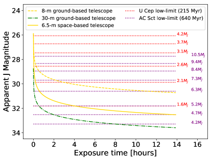
Figure 5: Comparison of simulated SL planet $J$-band magnitude with observational detection limits, as a function of exposure time and planet mass. We consider different observational capabilities corresponding to some of the technology regions in Figure 4: a current 8-m (yellow dashed line) and a future 30-m (green dot-dashed) ground-based telescope and a near-future 6.5-m (yellow dashed) space facility. We assume photon-limited detections and require a signal-to-noise ratio of 10. For the ground-based observatories, we adopt an overall efficiency of 20% and a sky background contamination of $16.7\;\text{mag}/\text{arcsec}^{2}$. For the space-based case, we assume a 30% efficiency and a zodiacal background contamination of $22.2\;\text{mag}/\text{arcsec}^{2}$. SL planet magnitudes are calculated at the distances of U Cep (red) and AC Sct (purple). Around U Cep, within a 1 hour exposure, a $\gtrsim 4.5M_{J}$ planet is detectable with current ground-based or near-future space-based instruments, a $\sim$1.5$M_{J}$ planet with future ground-based facilities. Around AC Sct, these limits rise to $\sim$9$M_{J}$ and 6-8$M_{J}$, respectively.

The eclipse durations and short orbital periods of U Cep and AC Sct allow for efficient scheduling of their observations. Ideally, the duration of totality would exceed the exposure time required for planet detection and the eclipses would be frequent enough to allow for repeat observations during a typical observing run of several nights. As discussed above, a $\sim$1 hour exposure is required to detect planets around U Cep and AC Sct with current ground- or near-future space-based facilities. In comparison, the totality of the primary eclipse for U Cep lasts 90 minutes, during a primary eclipse of 9.0 hours that occurs every 2.5 days. For AC Sct, totality lasts approximately 168 minutes, during a primary eclipse of 16.1 hours every 4.8 days. Therefore, we can achieve the detection limit within a reasonable time frame.

In Figure 6, we compare the properties of U Cep and AC Sct (Table 1) with those of binaries known to host exoplanets (Schwarz et al., 2016), regardless of the detection technique. Our eclipsing binary targets have earlier type primaries and larger total masses due to the Dmag and age criteria applied above. Specifically, among the 97 binaries known to host planets and whose primaries have been spectrally classified (Schwarz et al., 2016), there are none with B- or A-type primaries or with total masses above 4$M_{\odot}$ like our targets. Thus, targeting our binaries would expand the spectral and total mass ranges of host binaries, were planets discovered there.

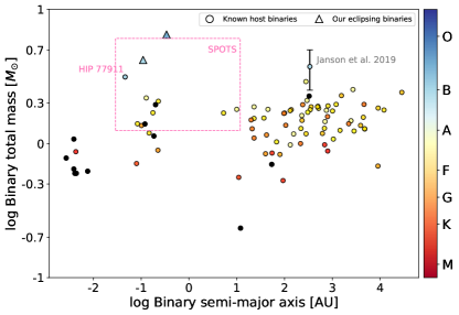
Figure 6: Binary total mass versus semi-major axis plane comparing our two best eclipsing binary targets, U Cep and AC Sct, with binaries known to host planets (Schwarz et al., 2016). The datapoints are color-coded by primary spectral type; black dots are systems whose primary type is not available. As a consequence of our Dmag and binary age selection criteria, U Cep and AC Sct have earlier type primaries and larger total masses than typical for known host binaries. This distinction would expand the parameter space of SL hosting binaries, were planets discovered in our target systems. We highlight HIP 79098 AB (gray), which has a candidate substellar companion (Janson et al., 2019) and HIP 77911 (pink), which has a candidate planetary-mass companion (Asensio-Torres et al., 2018); these systems have primaries with similar spectral types to our targets, but lower total masses. In comparison to the parameter boundaries of the SPOTS survey (Asensio-Torres et al., 2018) (pink box), our targets fall on the low side of the semi-major axis distribution and the high end of total mass.

4 Searching for Reflected Light Planets

Of the few direct imaging detections around binaries so far, none has included a RL planet. Therefore, it is interesting to test whether our approach would give access to this unexplored territory. There is an added benefit to using eclipsing binaries for RL planets relative to SL ones. At eclipse, the planet-star contrast is improved, while the RL planet is still brightened by the light of both binary components. RL planets have evolved and cooled, so, unlike for SL planets, there is no age constraint for shortlisting targets here.

Table 2: Best Eclipsing Binary Targets for Direct Detection of Reflected Light Exoplanets

Name	$m$	Dmag	Filter	$m_{V}$	d	Period	t${}_{\text{Dmag}}$	Spec Type
					[pc]	[days]	[min]
RR Cae	14.88	3.30	$B$	14.40	21.21	0.3	11	WD+M5-6V
V1412 Aql	15.67	2.63	$V$	15.67	22.93	$\cdots$	$\cdots$	DC7
RT Pic	9.90	2.60	$p$	9.07	54.39	$\cdots$	$\cdots$	G8V

In selecting potential RL targets, the main observational limitation is the distance of the binary from us. Given that a typical inner working angle of current coronagraphs (yellow region; Figure 7) is on the order of 100 mas, we do not expect to observe RL planets on tight orbits in faraway systems. At 50 pc away, the separation corresponding to a planet on a 1 AU orbit is only 20 mas, whereas an orbit of 5 AU or larger is observable. Therefore, we consider only the three deep (Dmag $\gtrsim$ 2.5) eclipsing binaries within roughly 50 pc: V1412 Aql at 22.9 pc, RR Cae at 21.2 pc, and RT Pic at 54.4 pc (Table 2). In the case of RR Cae, a $4.2\;M_{J}$ planet has already been discovered via the eclipse timing method at $5\;\text{AU}$ (Qian et al., 2012b).

For RR Cae (11 min totality, $\sim$14 min eclipse duration, 7.2 hour orbital period), there is little time during totality for observations, but we can build up a long exposure by observing for a short fraction of each night over multiple nights. For the other two targets, the totality, eclipse duration, and binary period are not known at present.

To determine whether an RL planet is detectable for these binaries, we build the observational space in Figure 7 as in Figure 1. We assume that Jupiter- and Venus-like planets (i.e., with the same sizes and albedos as the originals) have observed planet-star separations of at least 20 mas, the detectable angular separation limit of future technology (green and dark blue regions in the figure). We implicitly assume that these simulated planets could lie this physically close to their binary. The separation between the binary components is not available in the literature; therefore, we cannot predict whether the planets lie on a P- or S-type orbit.

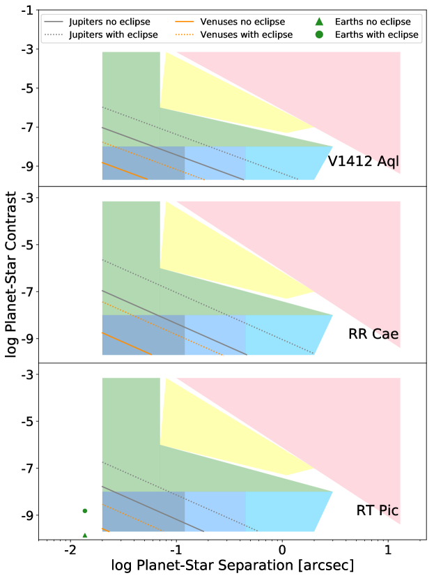
Figure 7: Testing the detectability of RL planets during the eclipse of the binary. Once again, we plot the observational space from Figure 1, but now for the closest eclipsing binaries in our sample. We consider simulated Jupiter- (gray) and Venus-like (orange) planets at increasing separations from the hosts, starting from 20 mas, the detectable angular separation limit of near-future facilities (green and dark blue regions). We plot the $V$-band contrasts both during (dotted lines) and before/after the eclipse (solid lines). The planet flux observed would decline from left to right. A habitable (i.e., flux received from the binary equal to the solar constant) Earth-like (same radius and albedo) planet only appears on this plot for RT Pic, at eclipse (green circle) and at other times (green triangle). The planet-star contrasts and separations of “Jupiters” and “Venuses” orbiting our closest binaries are accessible with future ground- and space-based coronagraphs. While the contrast of the habitable Earth-like planet around RT Pic is achievable with planned space-based instruments, the planet-star separation is too small.

For each binary, we derive the planet-star contrast at maximum binary brightness (L${}_{\text{pl}}/$L_V) and during the eclipse (L${}_{\text{pl}}/$L_V,e) in the $V$-band. The luminosity at eclipse (L_V,e) is estimated from Eq. 5 using the $V$-band luminosity outside eclipse (L_V) and the observed Dmag, which is reported in other photometric filters for RR Cae ($B$) and RT Pic ($p$) (see Table 2). Unlike in Section 3.2, we do not have enough information here about the primary and secondary (i.e., spectral type and/or color), and so cannot convert Dmag to a common band. Given that Dmag may decrease with increasing wavelength, the plotted contrast boost could be overestimated for RR Cae and RT Pic.

The luminosity of the planet due to reflection (L${}_{\text{pl}}$) is obtained from the definition of the albedo. Assuming the planet to be a disk of radius R${}_{\text{pl}}$ and manipulating the ratio between the incident and reflected flux yields

$$\text{L}_{\text{pl}}=\text{L}_{\text{tot}}\frac{\text{R}_{\text{pl}}^{2}}{a^{2}}\frac{\alpha}{4},$$ (6)

where $a$ and $\alpha$ are the semi-major axis of the planetary orbit and the albedo, respectively. The values of $a$, $\alpha$, and R${}_{\text{pl}}$ are taken from the NASA fact sheets for each planet.

Figure 7 shows that for Jupiter- and Venus-like planets with planet-star separations within the technology limits, the planet-star contrasts also will be accessible.

To further quantify the detectability of these simulated RL planets, we estimate the required exposure times for future ground- (Figure 8) and space-based (Figure 9) observations, similarly to Figure 4. For ground-based and space-based imaging, respectively, we assume that the observations are carried out in the $J$- (1.25 $\mu m$) and $V$-band (555 nm) to achieve the best planet-star contrast and separation. For the ground-based case, a large telescope aperture ($\sim$30 m) with extreme-AO in the near-IR leads to the best contrast, given that extreme-AO in visible light is considerably more challenging.

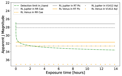
Figure 8: Comparison of simulated $J$-band magnitude with observational detection limit, as a function of exposure time. We assume a 30-m ground-based telescope with the same parameters as in Figure 5 (green dot-dashed line). Also plotted are the apparent magnitudes of a “Jupiter” and “Venus” at a separation of 20 mas from V1412 Aql (dotted gray and dotted orange lines, respectively), RR Cae (dashed gray and dashed orange lines), and RT Pic (solid gray and solid orange lines). RT Pic is the most promising target given the higher brightness of the planets there. A Jupiter-like planet around all three binaries and a Venus-like planet around RR Cae and RT Pic would be detected in two hours.

For a Jupiter-like planet at 20 mas separation, the $J$-band magnitude is brighter than 33 mag around all three eclipsing binaries, implying a ground-based detection within 2 hours (Figure 8). With a space-based telescope (Figure 9), a Jupiter around RT Pic would be detected in less than 1 hour with a 2-m aperture, in $\sim$4 hours around RR Cae with a 3-m aperture, and in $\sim$7 hours around V1412 Aql with a 5-m aperture. For a Venus-like planet at 20 mas separation, the $J$-band magnitude would be 37.1, 32.6, and 31.7 mag, respectively, for V1412 Aql, RR Cae, and RT Pic, requiring at most two hours to reach the detection limit around RR Cae and RT Pic with a ground-based telescope. With a space-based telescope, the $V$-band detection limit of a Venus would be accessible in less than 10 hours, even with a 4-m aperture, but only around RT Pic.

To Figure 7, we add an Earth-like (same radius and albedo) planet, assuming that it is habitable, i.e., that the bolometric flux it receives from the binary is equal to the solar constant. Therefore, the semi-major axis of the planet is obtained from $\sqrt{\text{L}_{tot}}$ in AU. We do not consider the eccentricity of the binary or the gravitational interaction as the secondary moves in its orbit, both of which alter the habitable zone boundaries over time (Haghighipour, & Kaltenegger, 2013; Kaltenegger, & Haghighipour, 2013; Jaime et al., 2014).

While the “Earth” in RT Pic lies at a planet-star contrast detectable by space-based telescopes planned for the 2030’s, its separation from the binary is beyond the capability of those instruments. Indeed, the planet-star separation would be 13 mas, the planet-star $V$-band contrast $1.5\times 10^{-9}$ during the eclipse, and the planet $J$-band magnitude 32.4 and $V$-band magnitude 33.7. The detection limit in the $J$-band would be achievable in $\sim$2 hours with a ground-based telescope and in the $V$-band in $<$7 hours with a 6- to 8-m space-based telescope. For the ground-based case, the $1.5\times 10^{-9}$ planet-star contrast is not achievable. For the space-based telescopes, the diffraction limits are 23.3 mas ($\lambda$ = 555 nm, D = 6 m) and 17.5 mas ($\lambda$ = 555 nm, D = 8 m). Detection at 13 mas would require that the $1.5\times 10^{-9}$ planet-star contrast be achieved at 0.56 $\lambda$/D and 0.74 $\lambda$/D, respectively. Coronagraphs currently deliver deep contrast levels at $\gtrsim$2 $\lambda$/D (Guyon et al., 2006), so detecting an Earth-like planet around an eclipsing binary will require larger apertures and/or further advances in coronagraph technologies.

5 Advantages of our method and targets

As discussed in the previous section, for reflected light planets, the eclipse improves the observed planet-star contrast by dimming the primary while the planet remains illuminated by both stars. Observing eclipsing binaries has several other advantages for directly imaging both SL and RL planets: 1) The reduction of the binary to a point-like source during eclipse makes coronagraphy feasible. 2) The increase in planet-star contrast during eclipse makes fainter planets accessible. 3) The contrast boost allows detection of planets in intrinsically brighter, and thus more massive, stellar systems.

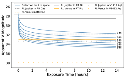
Figure 9: Comparison of simulated $V$-band magnitude with observational detection limit, as a function of exposure time, for the Venus- and Jupiter-like planets in Figure 8, assuming future space-based telescopes of different apertures and same parameters as the space-based case in Figure 5 (blue solid lines). The Venus-like planet (orange) around RT Pic would be detected in the $V$-band in less than 10 hours with a 4-m telescope. A Jupiter-like planet (gray) around RT Pic would be observable in less than 1 hour with a 2-m aperture, in $\sim$4 hours around RR Cae with a 3-m aperture, and in $\sim$7 hours around V1412 Aql with a 5-m aperture.

Eclipsing binaries are observable with a coronagraph, which would block the point-like light of the superimposed stellar components during the eclipse. In this way, our method incorporates both a natural starshade (the eclipse) and a man-made coronagraphic measurement. Light leakage during the coronagraphic measurement would be minimized, because it is possible to predict the time and duration of the binary eclipse accurately. In fact, one of our eclipsing binaries, RR Cae, has been successfully targeted in an exoplanet search with the eclipse timing variation technique (Qian et al., 2012b), for which timing accuracies on the order of seconds are required (Sybilski et al., 2010)

Our method would work best during the total eclipse of the primary, when the binary is point-like and darkest. However, we could still observe at partial eclipse, provided that the angular separation between the binary components is below the angular stellar size tolerance of the coronagraph (on the order of 0.1 $\lambda$/D). For our best SL targets (U Cep and AC Sct), the projected binary separation is $\sim$0.01 $\lambda$/D in the $J$-band with a 30-m telescope. Thus, observations during partial eclipse are potentially useful. For our best RL targets (V1412 Aql, RR Cae, and RT Pic), we lack sufficient information to infer the binary separations and make a similar evaluation.

The performance of a coronagraph with a small IWA ($<$3 $\lambda$/D) degrades with increasing stellar angular size (Guyon et al., 2006), even if the source size is well below the diffraction limit; light leakage is significantly higher for a partially resolved stellar disk than it would be for an on-axis point source. A shaped pupil could be used instead, but the IWA would be greater than $\sim$3 $\lambda$/D, restricting the target distance at which observations of close-in orbits could be made.

How might our method expand the parameter space of detected exoplanet properties? We have considered binaries that dim by at least 2.5 mag during eclipse. As a result, at a given planet-star contrast and host intrinsic stellar luminosity, our approach allows direct imaging detection of a planet at least 10$\times$ fainter than one around a single host star or non-eclipsing binary system, at the same distance. Physically, for RL planets, 10$\times$ fainter could imply 0.1$\times$ planet albedo or 0.33$\times$ planet size or 3$\times$ planet-star separation (see Eq. 6).

Does our method allow access to different types of host stars or binaries than previously explored in exoplanet systems? The Catalogue of Exoplanets in Binary Systems (Schwarz et al., 2016) lists detailed properties for 97 binaries with exoplanets, at least five of which were directly imaged. Compared to these, our best target binaries for SL planets are more massive and have earlier-type primaries (i.e., B-type). This difference arises because we selected on higher total binary mass so that any SL planets would be young and therefore bright enough to be detectable.

In general, compared to single star and non-eclipsing binary systems at the same distance, planet luminosity, and planet-star contrast, our SL and RL target binaries would have stellar luminosities at least 10$\times$ brighter and thus stellar masses $\sim$2-3$\times$ greater, assuming the canonical main sequence mass-luminosity relation. Therefore, our approach could expand the boundaries of the host stellar mass parameter space. If more exoplanets are discovered around such massive primaries, there are implications for how such planets form and evolve around binaries (Janson et al., 2011, 2019).

6 Conclusions

We investigate the plausibility of a new approach for directly imaging exoplanets. Our idea is to use the eclipse event in eclipsing binary systems as a tool to boost the planet to star flux contrast, i.e., to exploit a natural starshade. During the eclipse, the binary is reduced to a point-like source, making coronagraphic observations possible.

We select 289 binaries where the depth of primary minimum Dmag is $>2.5$ mag, which boosts the planet-star contrast by more than a dex. Thus, at a given observed planet-star contrast and host intrinsic stellar luminosity, we can detect a planet $>10\times$ fainter in an eclipsing binary, during eclipse, than in other star systems at the same distance. Likewise, we can detect planets of a given intrinsic luminosity around systems whose intrinsic stellar luminosity is $>10\times$ brighter and whose stellar mass is $\sim 2$-$3\times$ greater. In other words, we could directly image exoplanets in a massive binary system at the same contrast level as in a lower mass one.

We consider using this method to detect self-luminous (SL) and reflected light (RL) planets around our binaries.

For the SL planet case, we determine whether 0.5 to 10 $M_{J}$ planets could be detected during eclipse with current or future coronagraphs. SL planets are easiest to detect in young systems, given that the thermal emission of the planet decreases with time. Therefore, we select on the age of the binary, as well as the infrared brightness of the planet at the distance of the binary and the planet-star contrast. Because we lack measured ages for our best target binaries, which are classical Algols, we use Algol models (van Rensbergen et al., 2010; Mennekens & Vanbeveren, 2017) to constrain a plausible age interval from the binary total mass.

Using these criteria, we identify two targets: U Cep and AC Sct. Around them, we might detect $\sim$4.5$M_{J}$ and $\sim$9$M_{J}$ SL planets with current ground- or near-future space-based instruments, respectively. With future ground-based facilities, these limits reduce to 3-4$M_{J}$ and 6-8$M_{J}$. Because of our Dmag $>2.5$ and age criteria, these targets possess larger total masses ($>4.2M_{J}$) and earlier-type (B7-, B9-) primaries than typical of known host binaries. As noted above, our method puts such massive stellar systems within the reach of coronagraphic observations; targeting these systems would expand the host stellar parameter space for testing SL planet formation and evolution.

For RL planets, the advantage of using eclipsing binaries is that both binary stars continue to illuminate the planet while the planet-star contrast is increased during the eclipse. To find the best targets in this case, we focus on only the nearest (within $\sim$50 pc) eclipsing binaries in our sample: RR Cae, V1412 Aql, and RT Pic, for which the contrast boost during eclipse is 1.32, 1.05, and 1.04 dex, respectively. We assume that a large (30-meter) ground-based telescope and intermediate (2- to 8-meter) space-based telescopes will be available in the future.

We consider a Jupiter-like, Venus-like, and habitable Earth-like planet, estimating the change in detection limit with exposure time in the $J$-band with future ground-based telescope and in the $V$-band with space telescopes. For a “Jupiter” at 20 mas in all three target binaries, a detection is achieved in less than $\sim$10 hours with the ground- and space-based telescopes, whereas for a “Venus” at 20 mas, detection is possible in the $J$-band around RR Cae and RT Pic and in the $V$-band around RT Pic. Thus, directly imaging these Jupiter- and Venus-like planets is within the capabilities of planned facilities.

Detection of a habitable Earth-like planet remains a challenge. In a less than $\sim$10 hour exposure in the $J$-band with the ground-based telescope or in the $V$-band with a 6- to 8-meter space telescope during the eclipse, this “Earth” would be bright enough to detect if it orbited RT Pic. The planet-star contrast of $1.5\times 10^{-9}$ would be achievable from space. The planet-star separation of 13 mas is equivalent to 0.56 $\lambda$/D and 0.74 $\lambda$/D for the future 6-m and 8-m space-based telescopes, respectively. Given that current coronagraphs deliver deep contrast levels at $\gtrsim$2 $\lambda$/D (Guyon et al., 2006), larger apertures and/or new coronagraph advances will be required for detection.

Appendix A Full Sample of Eclisping Binary Systems

Table 3:

Name	RA	Dec	$m$	Dmag	Filter	Ref	Flag	$\pi$	L${}_{\text{tot}}$	Spec Type	Evol Class
	[hh mm ss]	[dd mm ss]						[mas]	[$L_{\bigodot}$]
LQ Cas	00 04 10.9597	+61 42 07.875	14.10	3.10	p	M	0	0.62	5.21	$\cdots$	$\cdots$
V0411 Cas	00 30 11.2537	+56 07 47.734	13.90	2.80	B	M	0	0.50	11.64	$\cdots$	$\cdots$
CV Cas	00 31 54.4680	+71 41 38.638	13.90	3.60	p	M	0	0.86	8.23	$\cdots$	$\cdots$
GW And	00 35 09.4069	+41 40 03.465	14.60	2.80	B	M	0	0.28	$\cdots$	$\cdots$	$\cdots$
KQ Cas	00 38 37.6964	+58 32 42.210	14.10	2.90	p	M	0	0.31	20.36	$\cdots$	$\cdots$
UU And	00 43 45.0803	+30 56 19.664	11.20	3.00	V	B	0	1.06	10.35	F5+[K7IV]	SA
Y Hyi	00 45 50.6974	-78 49 16.812	10.40	3.60	VT	B	1	2.35	15.38	A6V+[K3IV]	SA
V Tuc	00 51 46.5986	-71 59 52.927	10.60	8.20	V	B	1	1.86	13.35	B9/A2IV+[G5IV]	SA
V0415 Cas	00 54 31.0203	+59 24 00.027	14.00	2.80	b	M	0	0.40	24.20	$\cdots$	$\cdots$
V0386 Cas	00 59 11.2667	+55 57 20.037	14.00	2.50	b	M	0	0.34	35.09	$\cdots$	$\cdots$
U Cep	01 02 18.4416	+81 52 32.080	6.86	2.54	VH	B	0	5.04	$\cdots$	B7Ve+B8III-IV	SA
FK And	01 07 03.1786	+37 29 04.825	14.00	2.80	p	M	0	0.30	$\cdots$	$\cdots$	$\cdots$
OY Per	01 34 53.7662	+53 39 31.606	15.00	2.50	p	M	0	0.33	9.28	$\cdots$	$\cdots$
BL Hyi	01 41 00.3995	-67 53 27.469	14.90	3.10	V	M	0	7.65	$\cdots$	WD+M3-V	S2C
V0367 Cas	01 41 11.2580	+61 15 35.226	14.20	3.10	b	M	0	0.48	12.53	$\cdots$	$\cdots$
GH Cas	01 49 03.3762	+56 16 26.817	12.30	3.50	p	M	0	0.87	16.72	F2	$\cdots$
HS Per	01 52 11.6089	+57 06 42.715	13.00	2.60	V	M	0	0.89	12.51	A0II-III	$\cdots$
XZ And	01 56 51.5242	+42 06 02.181	10.15	2.54	V	M	1	1.84	21.97	A1V+G5IV	SA
X Tri	02 00 33.7370	+27 53 19.205	8.55	2.72	V	B	1	4.82	$\cdots$	A5V+[G2IV]	SA
LL Per	02 14 51.5373	+57 29 34.456	17.00	2.50	p	M	0	0.22	$\cdots$	$\cdots$	$\cdots$
MO And	02 23 53.6676	+39 59 02.767	13.20	3.00	p	M	0	0.52	15.65	$\cdots$	$\cdots$
LM Per	02 23 56.6594	+56 17 19.310	16.00	2.50	p	M	0	0.21	$\cdots$	$\cdots$	$\cdots$
RW Tri	02 25 36.1555	+28 05 50.893	12.50	2.42	V	M	1	3.17	$\cdots$	WD+M0V	S2C
WW Hor	02 36 11.4500	-52 19 13.500	18.40	4.60	B	M	0	3.07	$\cdots$	WD+M6V	S2C
Z Per	02 40 03.2329	+42 11 57.694	9.70	2.70	p	M	0	1.40	42.94	A0V+G0IV-V	SA
V For	02 40 51.4000	-25 52 14.000	14.05	2.95	B	M	0	0.36	$\cdots$	$\cdots$	$\cdots$
V0366 Per	02 44 10.6082	+36 35 11.856	13.70	2.60	b	M	0	0.89	5.50	$\cdots$	$\cdots$
V0479 Per	02 46 05.6524	+43 17 07.679	14.40	3.50	b	M	0	0.12	$\cdots$	$\cdots$	$\cdots$
SS Cet	02 48 36.2797	+01 48 26.894	9.40	3.60	V	B	1	1.85	25.4	A0+[K0IV]	SA
LS Per	02 57 08.7937	+37 53 40.477	11.50	3.10	p	M	0	0.88	30.23	A7IV	$\cdots$
QU Per	03 05 54.6745	+40 41 12.625	12.20	2.60	p	M	0	0.54	33.60	A2Ve	$\cdots$
EF Eri	03 14 13.2527	-22 35 42.917	14.50	2.80	B	M	0	6.27	$\cdots$	WD+M9V	S2C
UZ For	03 35 28.6515	-25 44 21.765	18.20	2.70	V	M	0	4.17	$\cdots$	WD+M4.5V	S2C
WY Per	03 38 24.1599	+42 40 39.050	11.50	2.70	V	B	0	0.83	21.22	A0+[K25IV]	SA
GH Cam	03 41 31.4326	+67 04 43.571	13.80	3.20	B	M	0	0.43	15.70	$\cdots$	$\cdots$
HU Per	03 42 33.1687	+39 06 03.625	10.90	3.00	p	M	0	0.54	66.28	A	$\cdots$
RW Tau	04 03 54.3166	+28 07 33.498	8.00	3.80	VH	B	1	3.27	$\cdots$	B8Ve+K0IV	SA
RV Per	04 10 37.9975	+34 15 54.883	10.23	3.75	V	B	1	0.94	37.71	A2+[G7IV]	SA
V0407 Tau	04 10 58.4464	+26 18 21.620	13.50	3.00	b	M	0	0.40	$\cdots$	$\cdots$	$\cdots$
BN Tau	04 15 44.8807	+30 40 08.025	10.17	4.21	VT	B	1	0.73	16.43	A7+[K2IV]	S
RR Cae	04 21 05.5631	-48 39 07.062	14.88	3.30	B	M	0	47.16	$\cdots$	WD+M5-6V	DW
TZ Eri	04 21 40.3306	-06 01 09.201	9.80	2.80	V	B	0	3.30	10.41	F3+[K5IV]	SA
AO Eri	04 32 00.9396	-17 44 47.651	10.30	3.27	VT	B	1	1.40	19.17	A8+[G8IV]	S
AC Tau	04 37 06.3566	+01 41 31.158	10.30	2.80	V	B	0	1.77	10.44	F0+[K6IV]	SA
AQ Cam	04 51 17.8661	+54 55 59.950	12.00	4.00	p	M	0	0.23	$\cdots$	B7	$\cdots$
ET Ori	04 55 34.3335	+01 22 49.564	10.13	3.14	VT	B	1	2.75	5.87	G3+[K3IV]	SA
EQ Ori	04 57 14.4652	-03 36 04.657	10.20	3.10	P	B	0	1.65	$\cdots$	A0+[G2IV]	SA
V0723 Tau	05 06 46.1891	+28 35 23.410	14.50	2.60	b	M	0	0.60	4.30	$\cdots$	$\cdots$
FL Ori	05 07 46.6517	-02 44 38.247	11.40	3.20	P	B	0	1.98	5.91	A3V+[K0IV]	SA
XZ Cam	05 17 12.6742	+75 50 05.354	11.40	3.00	VT	B	0	0.81	42.44	A0+[K0.5	SA
V0666 Ori	05 54 06.5077	+17 56 18.152	14.00	3.00	b	M	0	0.75	9.84	$\cdots$	$\cdots$
RT Pic	06 00 41.2987	-44 53 50.106	9.90	2.60	p	M	0	18.39	0.62	G8V	$\cdots$
LP Gem	06 05 05.1282	+26 40 53.386	12.50	2.50	p	M	0	0.53	35.88	$\cdots$	$\cdots$
DX Ori	06 05 44.7518	+08 20 55.289	13.50	2.50	p	M	0	0.41	17.11	$\cdots$	$\cdots$
CG Pup	06 07 02.9478	-46 44 47.717	10.20	2.80	p	M	0	2.05	5.81	$\cdots$	$\cdots$
V0347 Pup	06 10 33.6585	-48 44 25.363	13.55	2.40	B	M	0	3.38	0.28	$\cdots$	$\cdots$
RU CMa	06 22 33.5874	-22 41 29.151	11.30	2.50	V	M	1	1.36	$\cdots$	$\cdots$	$\cdots$
BO Gem	06 25 01.2975	+17 58 12.777	11.30	3.80	P	B	1	1.12	21.10	A2+[K3IV]	SA
NS CMa	06 29 09.5867	-31 15 33.800	14.00	2.71	V	M	0	0.40	10.97	$\cdots$	$\cdots$
V0639 Mon	06 37 20.1591	+11 36 31.485	16.00	2.50	b	M	0	0.31	$\cdots$	$\cdots$	$\cdots$
MP Gem	06 48 33.4000	+19 37 15.000	15.40	2.60	p	M	0	0.41	$\cdots$	$\cdots$	$\cdots$
EF Gem	06 51 01.8159	+17 29 54.987	12.60	2.80	p	M	0	0.41	36.42	$\cdots$	$\cdots$
CH Mon	06 51 38.1214	+05 56 12.268	13.10	2.80	p	M	0	0.57	17.73	$\cdots$	$\cdots$
EH Mon	06 52 08.7658	-07 03 52.971	13.80	2.50	p	M	0	0.19	$\cdots$	$\cdots$	$\cdots$
RV Lyn	06 56 11.4299	+50 51 45.509	13.00	2.60	p	M	0	0.66	12.38	$\cdots$	$\cdots$
BP Mon	06 56 55.4325	+05 01 43.820	13.10	2.60	p	M	0	0.74	11.06	$\cdots$	$\cdots$
FS Gem	06 57 21.2259	+16 30 13.681	13.70	2.90	p	M	0	0.25	$\cdots$	$\cdots$	$\cdots$
UU CMa	06 58 41.4546	-18 48 48.187	10.00	2.50	p	M	0	1.79	9.93	$\cdots$	$\cdots$
AC CMa	07 08 23.2400	-19 40 01.547	12.80	2.50	p	M	0	0.75	17.91	$\cdots$	$\cdots$
AB CMi	07 07 57.3118	+11 58 18.883	13.40	2.50	p	M	0	0.26	$\cdots$	$\cdots$	$\cdots$
HO Mon	07 10 19.2100	+00 25 28.949	11.40	2.80	P	B	0	1.05	22.02	A5+[K2.5IV]	SA
AQ Mon	07 14 17.6748	-07 13 45.060	9.79	2.71	VT	B	1	1.48	21.39	A0+[A4.5]	SA
FP Mon	07 15 08.8358	-09 57 47.639	13.30	3.00	p	M	0	0.85	7.05	F6V	$\cdots$
AF CMa	07 15 22.7708	-23 40 42.624	12.30	3.20	p	M	0	0.67	33.76	$\cdots$	$\cdots$
HS Cam	07 19 14.5151	+65 57 44.305	19.40	4.00	B	M	0	2.19	$\cdots$	WD+M4-6V	S2C
RY CMi	07 22 58.1591	+06 46 35.019	11.90	3.00	p	M	0	0.55	$\cdots$	$\cdots$	S
CX Pup	07 41 53.5171	-22 53 36.924	12.20	3.00	p	M	0	0.84	$\cdots$	$\cdots$	$\cdots$
V0681 Mon	07 52 21.9573	-01 17 25.149	13.00	2.50	b	M	0	0.81	16.18	$\cdots$	$\cdots$
TU Mon	07 53 19.7487	-03 02 31.137	9.00	2.70	VH	B	1	0.61	$\cdots$	B5V+A5III:	SH
MT Pup	07 54 11.8928	-14 39 16.633	15.00	4.00	p	M	0	1.01	$\cdots$	em	$\cdots$
FG Pup	08 04 31.6979	-24 02 53.406	13.00	3.00	p	M	0	0.46	22.14	$\cdots$	$\cdots$
IO Pup	08 06 57.9454	-25 49 08.288	13.50	2.50	p	M	0	0.48	$\cdots$	$\cdots$	$\cdots$
AV Vel	08 07 01.3411	-47 38 46.007	11.90	2.70	p	M	0	0.89	14.32	$\cdots$	$\cdots$
FI Pup	08 08 14.7308	-20 17 14.882	14.00	2.50	p	M	0	0.24	$\cdots$	$\cdots$	$\cdots$
XZ Pup	08 13 31.0553	-23 57 11.387	7.75	2.51	V	M	1	2.54	$\cdots$	A0	SA
FQ Pup	08 18 10.5357	-23 48 40.571	14.00	2.50	p	M	0	0.43	8.11	$\cdots$	$\cdots$
FR Pup	08 21 19.9553	-22 18 45.703	13.50	3.00	p	M	0	0.27	$\cdots$	$\cdots$	$\cdots$
DR Lyn	08 24 24.4675	+50 00 50.891	11.60	2.70	V	M	0	1.24	6.42	$\cdots$	$\cdots$
DE Hya	08 27 47.5470	+05 38 58.939	11.00	3.00	V	B	0	$\cdots$	$\cdots$	A2+[K2IV]	SA
SY Hya	08 29 51.6786	-09 23 57.496	10.70	2.90	VT	B	0	0.93	$\cdots$	A5+[K2IV]	SA
VW Hya	08 33 51.0321	-14 39 53.891	10.50	3.60	V	B	1	0.80	$\cdots$	A3+[G4IV]	SA
RY Cnc	08 39 54.6211	+19 49 18.864	12.99	2.53	V	B	0	0.85	7.46	B8+[G5IV]	S
TY Cnc	08 47 09.6962	+08 24 24.582	12.70	3.00	p	M	0	0.69	$\cdots$	$\cdots$	$\cdots$
TU Cnc	08 52 16.6529	+09 05 18.781	9.90	2.50	P	B	0	1.42	28.54	A0+[G8	SA
AC UMa	08 55 54.1228	+64 58 14.999	10.30	3.70	V	B	0	1.24	41.14	A2+[K6IV]	SA
RX Hya	09 05 41.1657	-08 15 39.727	8.90	2.70	V	B	0	3.71	8.98	A8+[K5IV]	SA
TY Hya	09 29 02.3991	+05 34 28.269	10.50	3.00	P	B	0	0.76	37.79	A0+[K1IV]	SA
Y Leo	09 36 51.8058	+26 13 57.643	10.09	3.11	V	M	1	2.49	11.94	A5V+K5V	SA
DX Vel	09 51 45.9871	-50 53 23.716	10.08	3.42	VT	B	1	1.85	12.12	A5+[G1IV]	SA
IV Car	10 02 36.6688	-58 57 22.460	11.30	2.80	p	M	0	1.29	$\cdots$	$\cdots$	$\cdots$
HL Car	10 04 42.7497	-61 50 35.084	11.00	3.00	p	M	0	0.77	53.09	$\cdots$	$\cdots$
TT Vel	10 20 16.4606	-46 14 04.436	10.10	3.24	VT	B	1	1.95	12.54	A5+[F8.5]	SA
AW Car	10 32 35.0208	-60 46 10.653	12.20	4.30	p	M	0	0.34	39.11	A3	$\cdots$
FV Car	10 42 31.9233	-61 57 55.072	12.90	2.90	p	M	0	0.57	60.55	$\cdots$	S
PT Car	11 03 17.6000	-74 56 37.000	12.80	3.20	p	M	0	$\cdots$	$\cdots$	$\cdots$	$\cdots$
EH Car	11 04 23.8163	-61 18 23.020	12.50	2.50	p	M	0	0.30	47.39	$\cdots$	$\cdots$
AN UMa	11 04 25.6556	+45 03 13.941	14.90	5.30	B	M	0	3.10	$\cdots$	$\cdots$	S2C
DE Car	11 06 13.6515	-60 47 32.672	11.20	2.60	p	M	1	0.94	17.85	A	SA
V0443 Cen	11 25 22.5000	-59 37 40.000	12.80	2.50	b	M	0	$\cdots$	$\cdots$	$\cdots$	$\cdots$
AB Cen	11 26 21.2641	-58 24 58.136	10.60	2.60	p	M	0	0.62	85.93	G0	$\cdots$
V0646 Cen	11 36 58.7768	-53 12 35.414	9.00	2.70	b	M	0	1.40	$\cdots$	B8IV	S
V0348 Cen	11 48 28.9566	-43 46 53.264	10.70	2.70	b	M	0	1.26	14.73	A	$\cdots$
Z Crv	12 29 41.7139	-23 38 03.878	14.00	2.50	V	M	0	1.21	1.32	$\cdots$	$\cdots$
RR Crv	12 30 26.9456	-17 58 53.449	11.10	2.80	p	M	0	1.33	12.15	$\cdots$	$\cdots$
BP Mus	12 50 37.7277	-71 46 18.698	9.60	3.00	V	M	0	1.75	21.65	A0,5/1,5V+G5III	$\cdots$
CT Cen	13 10 43.0552	-58 16 38.629	10.30	2.70	p	M	0	1.56	41.87	A3(ea)	SA
CY Cen	13 12 13.0891	-52 52 51.852	13.30	2.80	p	M	0	0.70	6.89	$\cdots$	$\cdots$
UW Vir	13 15 20.7356	-17 28 16.924	8.84	3.16	V	B	0	4.27	10.35	A4+[K3IV]	SA
BM Cen	13 17 38.4543	-56 17 09.765	13.20	2.80	p	M	0	0.69	7.51	$\cdots$	$\cdots$
BP Cen	13 19 08.6963	-49 55 04.751	12.20	3.80	p	M	0	1.14	$\cdots$	$\cdots$	$\cdots$
SX Hya	13 44 37.3594	-26 46 48.376	8.60	4.00	VH	B	1	3.86	16.23	A3+[G9IV]	SA
IQ Cen	14 00 34.4391	-54 16 15.669	12.70	3.00	p	M	0	0.51	28.32	$\cdots$	$\cdots$
AN Cir	14 04 21.9000	-65 38 05.000	13.80	2.80	p	M	0	$\cdots$	$\cdots$	$\cdots$	$\cdots$
GK Vir	14 15 36.4126	+01 17 18.227	17.01	5.99	V	M	0	2.11	$\cdots$	DA0+M3-5V	DW
TU Lup	14 43 40.6725	-49 50 24.752	12.40	3.80	p	M	0	0.72	11.73	$\cdots$	$\cdots$
W Cir	15 11 47.0000	-55 38 12.000	13.80	2.70	b	M	0	$\cdots$	$\cdots$	$\cdots$	$\cdots$
EV Lup	15 16 08.0026	-44 19 20.380	9.80	2.70	p	M	0	1.05	33.65	$\cdots$	$\cdots$
TW Dra	15 33 51.0598	+63 54 25.706	8.00	2.50	p	M	1	6.01	22.75	A8V+K0III	SA
LX Ser	15 38 00.0940	+18 52 03.246	13.30	4.10	B	M	0	2.03	$\cdots$	WD+M32V	S2C
HH Nor	15 43 30.1810	-51 50 47.542	9.70	3.05	VT	B	1	2.22	15.31	A3+[G8IV]	S
YY Nor	15 47 58.4618	-57 24 42.626	13.20	2.90	p	M	0	0.76	12.13	$\cdots$	$\cdots$
HK Nor	15 58 54.7069	-51 41 54.960	12.60	2.60	p	M	0	0.88	3.69	$\cdots$	$\cdots$
HS Nor	16 01 44.9307	-57 27 33.167	12.60	2.60	p	M	0	0.41	25.41	$\cdots$	$\cdots$
BH Aps	16 08 40.2241	-76 50 28.071	10.80	2.60	p	M	0	1.00	$\cdots$	$\cdots$	$\cdots$
CE Nor	16 11 13.2040	-60 02 20.928	11.50	3.00	p	M	0	0.60	$\cdots$	$\cdots$	$\cdots$
CC Her	16 17 38.8937	+08 56 02.610	10.20	2.90	p	M	0	2.82	10.18	A1V(pSr)	SA
UU Nor	16 20 21.5635	-53 44 52.236	11.60	2.70	p	M	0	0.37	78.91	$\cdots$	$\cdots$
V0704 Ara	16 56 16.9143	-55 27 58.361	12.90	2.70	b	M	0	0.46	13.09	$\cdots$	$\cdots$
UU Oph	16 57 22.6406	-25 47 58.563	10.00	2.50	VH	B	0	0.76	$\cdots$	A0+[K2IV]	SA
V0588 Sco	16 57 49.7872	-40 29 59.953	14.00	2.50	b	M	0	0.58	7.09	$\cdots$	$\cdots$
V0416 Ara	16 58 06.6680	-55 30 12.252	12.60	2.90	b	M	0	0.36	28.39	$\cdots$	$\cdots$
IM Sco	17 00 13.2531	-31 27 57.609	13.30	3.20	p	M	0	0.64	4.29	G2V	$\cdots$
V1194 Oph	17 00 21.1176	-21 51 22.343	17.60	2.70	p	M	0	0.24	$\cdots$	$\cdots$	$\cdots$
V735 Oph	17 07 48.9680	+09 33 09.206	10.30	2.96	VT	B	0	1.78	11.25	A0+[G1IV]	SA
V0460 Sco	17 08 50.4000	-32 54 05.000	13.40	2.60	b	M	0	$\cdots$	$\cdots$	$\cdots$	$\cdots$
V1453 Oph	17 08 52.7155	-19 01 08.933	17.40	3.00	p	M	0	0.30	$\cdots$	$\cdots$	$\cdots$
FT Sco	17 10 55.2000	-32 41 09.000	13.80	2.70	p	M	0	$\cdots$	$\cdots$	$\cdots$	$\cdots$
V1578 Oph	17 12 14.2156	-20 14 54.864	16.40	3.40	p	M	0	0.11	$\cdots$	$\cdots$	$\cdots$
V1590 Oph	17 12 22.2904	-16 24 34.019	16.00	2.90	p	M	0	0.26	$\cdots$	$\cdots$	$\cdots$
TU Her	17 13 35.3658	+30 42 36.042	10.88	2.82	V	M	1	1.96	9.10	F0III/IV	SA
V0621 Sco	17 14 36.8000	-41 04 15.000	12.30	2.70	b	M	0	$\cdots$	$\cdots$	$\cdots$	$\cdots$
V0441 Oph	17 20 52.7094	-17 20 05.261	11.60	3.00	b	M	0	1.26	16.83	A0	$\cdots$
LT Ara	17 22 30.1256	-47 04 02.989	10.80	4.60	p	M	0	0.87	39.25	A	$\cdots$
V0506 Sco	17 23 12.4000	-39 11 40.000	13.30	2.70	b	M	0	1.02	$\cdots$	$\cdots$	$\cdots$
V0510 Sco	17 27 37.2557	-42 58 53.276	13.10	3.00	b	M	0	0.42	35.92	$\cdots$	$\cdots$
V0511 Sco	17 28 22.5406	-42 02 39.060	12.50	3.50	b	M	0	0.79	18.64	$\cdots$	$\cdots$
V0532 Oph	17 32 42.6073	-21 51 40.760	12.60	2.90	b	M	0	0.17	$\cdots$	$\cdots$	$\cdots$
RW Ara	17 34 49.2233	-57 08 50.566	8.85	2.60	V	M	1	2.53	$\cdots$	A1IV	SA
V0525 Sco	17 39 57.7671	-40 29 13.385	13.80	2.60	b	M	0	0.58	11.51	$\cdots$	$\cdots$
V0529 Oph	17 41 56.6000	-28 18 10.000	13.20	3.30	b	M	0	$\cdots$	$\cdots$	$\cdots$	$\cdots$
AK Ser	17 42 04.4088	-13 53 11.971	10.80	2.80	p	M	1	1.33	$\cdots$	A5	SA
V0755 Sgr	17 48 46.1804	-25 53 09.993	13.50	2.50	b	M	0	0.61	$\cdots$	$\cdots$	$\cdots$
V0765 Sgr	17 51 54.0858	-28 26 32.028	12.80	3.70	b	M	0	0.37	46.29	$\cdots$	$\cdots$
V913 Oph	17 55 03.5918	+14 10 39.254	11.50	3.00	P	B	0	2.14	5.19	A5+[G5IV]	SA
V391 Oph	17 58 09.1304	+04 39 27.610	11.50	3.50	P	B	1	0.70	12.93	A1+[G5IV]	SA
V2301 Oph	18 00 35.5318	+08 10 13.920	16.00	6.00	V	M	0	8.24	$\cdots$	WD+M6V	S2C
V0573 Oph	18 06 05.3800	+02 05 43.828	13.10	3.00	b	M	0	0.48	19.51	$\cdots$	$\cdots$
V1178 Sgr	18 11 03.8499	-30 30 56.884	12.80	2.50	p	M	0	0.08	$\cdots$	$\cdots$	$\cdots$
AG Pav	18 12 25.6276	-62 33 21.859	10.20	2.80	p	M	0	1.62	10.48	$\cdots$	$\cdots$
V1282 Sgr	18 13 34.6857	-34 28 42.944	11.90	4.30	p	M	0	1.08	13.03	$\cdots$	$\cdots$
V1959 Sgr	18 16 43.0576	-25 31 20.268	12.60	3.20	p	M	0	0.52	13.03	$\cdots$	$\cdots$
AI Sgr	18 16 45.0943	-21 34 48.529	11.80	3.20	p	M	0	0.43	87.41	$\cdots$	$\cdots$
V0710 Sgr	18 16 46.8091	-36 25 32.160	13.30	3.00	b	M	0	0.51	$\cdots$	$\cdots$	$\cdots$
V3171 Sgr	18 22 44.2273	-34 13 32.205	16.00	3.20	p	M	0	0.16	$\cdots$	$\cdots$	$\cdots$
V2537 Sgr	18 23 00.307	-32 34 03.030	12.30	2.50	p	M	0	$\cdots$	$\cdots$	$\cdots$	$\cdots$
V1654 Sgr	18 23 17.1000	-23 15 10.000	13.20	2.60	p	M	0	$\cdots$	$\cdots$	$\cdots$	$\cdots$
V0586 Oph	18 27 13.9427	04 17 15.319	13.30	2.50	b	M	0	0.77	14.19	$\cdots$	$\cdots$
V3421 Sgr	18 29 11.6135	-32 23 55.711	16.50	2.60	p	M	0	0.28	$\cdots$	$\cdots$	$\cdots$
V3476 Sgr	18 30 49.5100	-32 57 51.000	14.90	2.50	p	M	0	$\cdots$	$\cdots$	$\cdots$	$\cdots$
EY Ser	18 30 49.8137	+05 30 17.629	14.50	3.00	p	M	0	0.54	12.60	$\cdots$	$\cdots$
V4727 Sgr	18 33 30.7141	-28 58 51.239	10.60	3.20	V	M	0	1.15	14.61	$\cdots$	$\cdots$
V3622 Sgr	18 35 46.2499	-34 52 30.616	14.80	3.00	p	M	0	0.21	$\cdots$	$\cdots$	$\cdots$
V0372 Sct	18 38 03.6563	-04 01 06.118	14.20	2.60	b	M	0	0.35	54.58	$\cdots$	$\cdots$
V3696 Sgr	18 38 46.8768	-34 39 03.802	16.30	3.00	p	M	0	0.23	$\cdots$	$\cdots$	$\cdots$
BO Her	18 40 30.0965	+24 55 42.768	10.70	3.10	V	M	1	1.29	17.08	A7V	SA
V3752 Sgr	18 40 43.9834	-35 32 26.340	15.90	2.60	p	M	0	0.29	$\cdots$	$\cdots$	$\cdots$
RR Dra	18 41 47.4012	+62 40 34.944	10.00	3.30	V	B	0	2.17	20.23	A2+[G8IV]	SA
V1933 Sgr	18 45 10.1332	-19 47 19.960	12.50	2.50	p	M	0	0.62	22.20	$\cdots$	$\cdots$
AC Sct	18 46 01.4709	-10 14 55.815	10.00	2.60	V	B	0	1.01	63.82	B9+[G0IV]	SA
V0795 Aql	18 47 06.8639	+11 40 11.052	13.40	3.00	b	M	0	0.40	20.70	$\cdots$	$\cdots$
DH Her	18 47 34.5584	+22 50 45.795	9.40	2.60	V	M	1	0.33	$\cdots$	A5	SA
V0370 Sct	18 48 31.2299	-05 42 37.449	15.30	3.20	b	M	0	0.46	8.35	$\cdots$	$\cdots$
AD Her	18 50 00.3000	+20 43 16.509	9.38	10.74	V	B	1	1.71	37.58	A4V+[G9IV]	SA
FN Sct	18 50 46.7234	-05 12 07.916	12.70	2.50	B	M	0	0.35	108.38	B3Ve	$\cdots$
CT Sct	18 54 21.6365	-06 00 16.696	10.02	4.17	V	B	1	0.26	631.53	B7Vn+[A3]	SA
LP Her	18 55 41.2099	+12 15 28.400	13.00	3.20	p	M	0	0.65	16.56	$\cdots$	$\cdots$
EH Sct	18 57 39.7600	-06 52 59.700	14.80	2.70	p	M	0	$\cdots$	$\cdots$	$\cdots$	$\cdots$
BN Sct	18 58 42.8687	-08 20 28.364	11.40	3.20	p	M	0	0.82	44.06	A0Ib	$\cdots$
HY Aql	19 02 47.6109	-06 13 33.067	12.80	2.80	p	M	0	0.60	17.21	$\cdots$	$\cdots$
FK Aql	19 04 18.5775	+02 46 47.244	11.10	2.40	VT	B	0	1.38	19.77	B9+[G6IV]	SA
V1074 Sgr	19 05 23.6885	-18 47 06.864	12.70	2.50	p	M	0	1.26	7.49	F4III	$\cdots$
V1109 Aql	19 05 40.1991	+14 14 43.686	17.00	2.50	p	M	0	0.19	$\cdots$	$\cdots$	$\cdots$
EP Dra	19 07 06.1869	+69 08 43.874	17.60	2.90	V	M	0	2.59	$\cdots$	$\cdots$	S2C
V0413 Lyr	19 07 16.4316	+30 19 25.590	14.50	2.60	b	M	0	0.23	21.65	$\cdots$	$\cdots$
V0449 Lyr	19 07 37.0709	+44 00 19.797	12.50	3.50	b	M	0	0.18	$\cdots$	$\cdots$	$\cdots$
V0415 Sgr	19 07 37.0938	-23 37 08.543	12.30	3.00	b	M	0	0.55	38.86	$\cdots$	$\cdots$
V1112 Aql	19 07 39.1500	-00 23 07.100	14.00	2.50	p	M	0	$\cdots$	$\cdots$	$\cdots$	$\cdots$
KK Dra	19 07 56.6643	+59 23 52.065	11.80	3.00	V	M	0	1.69	3.63	$\cdots$	$\cdots$
V0407 Aql	19 11 10.8162	+01 08 52.145	13.30	2.50	b	M	0	1.24	4.33	$\cdots$	$\cdots$
NS Lyr	19 11 13.9662	+36 10 35.321	14.00	2.80	p	M	0	0.48	9.32	$\cdots$	$\cdots$
V354 Sgr	19 13 23.4427	-18 29 00.014	10.70	3.00	VT	B	1	1.50	19.05	F8+[K9IV]	SA
V1103 Cyg	19 14 57.6721	+46 10 01.622	15.00	2.50	p	M	0	0.30	10.29	$\cdots$	$\cdots$
RV Lyr	19 16 17.9644	+32 25 14.969	11.50	3.10	P	B	0	1.02	22.01	A5+[K3IV]	SA
YZ Aql	19 16 46.2253	-00 36 17.152	10.50	3.70	V	B	1	0.92	45.94	A3+[K5IV]	SA
V342 Aql	19 17 03.4768	+09 20 38.546	9.50	3.40	P	B	0	3.21	25.59	A4II+[K0IV]	SA
U Sge	19 18 48.4083	+19 36 37.720	6.50	2.60	V	B	1	3.62	$\cdots$	B8III+K	SA
FR Vul	19 36 24.8396	+26 45 56.558	9.91	2.54	VT	B	1	1.80	16.20	A2+[G7IV]	SA
V0418 Aql	19 36 39.4426	+03 57 00.470	12.80	3.20	b	M	0	1.06	6.72	$\cdots$	$\cdots$
LT Aql	19 38 49.7896	+06 34 59.039	12.40	2.50	p	M	0	0.59	30.27	B9III/IV	$\cdots$
V0932 Cyg	19 39 05.8610	+33 29 01.674	14.00	2.60	b	M	0	0.22	38.84	$\cdots$	$\cdots$
EN Cyg	19 40 09.4635	+29 16 23.100	12.90	3.20	p	M	0	1.06	7.76	$\cdots$	$\cdots$
V2168 Sgr	19 42 37.5266	-38 39 55.648	12.50	2.50	p	M	0	0.76	7.23	$\cdots$	$\cdots$
SY Cyg	19 46 34.3155	+32 42 18.463	10.70	3.50	P	B	0	0.94	39.95	A3+[K6IV]	SA
V1033 Aql	19 46 44.7712	+14 21 57.379	15.00	2.50	p	M	0	0.20	$\cdots$	$\cdots$	$\cdots$
V0814 Cyg	19 49 50.7520	+36 34 27.659	15.00	3.00	b	M	0	0.17	$\cdots$	$\cdots$	$\cdots$
V0689 Cyg	19 51 06.5892	+36 51 32.721	14.00	2.50	b	M	0	0.65	6.35	A5V	$\cdots$
V524 Sgr	19 53 14.5011	-14 54 38.882	9.96	2.54	VT	B	1	2.16	12.25	F8III+[K3IV]	SA
V0340 Aql	19 55 56.4890	+15 51 07.167	11.50	2.60	b	M	0	0.88	16.30	F	$\cdots$
BO Vul	19 56 29.0711	+23 54 45.011	10.50	2.80	p	M	0	2.79	9.76	F0+G0IV	SA
PV Cyg	19 56 29.1748	+37 43 09.124	12.70	2.80	p	M	0	0.58	13.71	A1	$\cdots$
V0691 Cyg	19 57 18.4468	+40 02 55.712	15.50	2.50	b	M	0	0.35	6.50	$\cdots$	$\cdots$
QT Cyg	19 58 07.3701	+38 49 27.887	14.80	2.60	p	M	0	0.26	15.77	A5	$\cdots$
V4140 Sgr	19 58 49.7022	-38 56 13.225	15.50	2.50	p	M	0	1.67	$\cdots$	WD+M6-7	S2C
QX Sge	19 59 36.7480	+20 48 14.599	20.40	2.60	V	M	0	$\cdots$	$\cdots$	$\cdots$	$\cdots$
V0698 Cyg	19 59 53.3495	+36 16 39.998	12.20	2.70	b	M	0	0.28	$\cdots$	B2	$\cdots$
V1174 Cyg	20 03 55.9791	+31 15 39.947	14.50	2.50	p	M	0	0.31	38.67	$\cdots$	$\cdots$
WW Cyg	20 04 02.7111	+41 35 16.462	10.02	3.24	V	B	0	0.80	$\cdots$	B7V+[G1IV]	SA
EX Vul	20 04 47.4096	+22 19 21.861	12.49	2.61	B	M	0	0.51	52.47	ea	$\cdots$
SW Cyg	20 06 57.9310	+46 17 58.147	9.24	2.59	V	M	1	2.12	33.46	A2e+K0	SA
V1037 Cyg	20 08 49.5433	+35 14 55.507	14.70	2.60	p	M	0	0.51	8.05	$\cdots$	$\cdots$
QY Aql	20 09 28.8293	+15 18 44.718	11.40	3.20	VH	B	0	0.78	57.18	F0+/K3IV/	SA
V1412 Aql	20 13 55.6789	+06 42 44.826	15.67	2.63	V	M	0	43.62	$\cdots$	DC7	$\cdots$
V0445 Aql	20 19 38.8300	+06 08 47.400	13.00	2.50	b	M	0	$\cdots$	$\cdots$	$\cdots$	$\cdots$
V Sge	20 20 14.6910	+21 06 17.17	8.60	5.30	V	M	0	0.42	$\cdots$	WN5	S2C
V1320 Cyg	20 21 22.0535	+39 19 57.924	15.90	2.60	p	M	0	0.44	14.06	$\cdots$	$\cdots$
V0445 Cyg	20 28 18.9582	+38 17 43.226	11.70	3.80	b	M	0	1.28	7.36	$\cdots$	$\cdots$
V1051 Cyg	20 31 00.5678	+56 46 31.159	14.40	2.80	p	M	0	0.52	5.52	$\cdots$	$\cdots$
LL Vul	20 31 43.3028	+25 38 36.303	16.00	3.00	p	M	0	0.09	$\cdots$	$\cdots$	$\cdots$
HN Del	20 33 45.1355	+11 03 40.875	14.50	2.50	p	M	0	0.59	4.96	$\cdots$	$\cdots$
SY Vul	20 36 21.8687	+23 51 51.038	13.00	3.00	p	M	0	0.28	29.26	$\cdots$	$\cdots$
KK Del	20 36 42.7618	+17 28 48.078	15.00	2.50	p	M	0	0.98	$\cdots$	$\cdots$	$\cdots$
W Del	20 37 40.0857	+18 17 03.752	9.69	2.64	V	M	1	1.23	$\cdots$	B9.5Ve+G5IV	SA
V1204 Cyg	20 44 10.7490	+46 49 03.756	14.50	3.00	p	M	0	0.48	6.93	$\cdots$	$\cdots$
V1843 Cyg	20 46 27.7000	+34 03 53.000	15.70	2.80	B	M	0	0.20	$\cdots$	$\cdots$	$\cdots$
V0398 Cyg	20 46 50.7555	+34 12 03.717	12.50	2.50	b	M	0	0.70	14.20	$\cdots$	$\cdots$
DW Cep	20 51 39.6899	+62 48 50.292	10.25	2.65	VT	B	1	1.21	20.02	B8+[F5]	SA
V1870 Cyg	20 51 41.0469	+35 44 08.101	14.30	2.90	B	M	0	0.86	4.37	$\cdots$	$\cdots$
V1884 Cyg	20 56 07.1165	+33 39 07.145	15.20	2.50	B	M	0	0.25	27.25	$\cdots$	$\cdots$
V1718 Cyg	21 02 01.2000	+41 31 57.000	14.70	2.80	p	M	0	$\cdots$	$\cdots$	$\cdots$	$\cdots$
V0377 Cyg	21 03 12.1952	+29 07 11.878	14.40	2.60	b	M	0	0.28	33.71	$\cdots$	$\cdots$
LY Del	21 06 26.0978	+19 24 36.422	10.40	3.10	V	M	0	0.54	129.27	$\cdots$	$\cdots$
V1539 Oph	21 11 20.0900	-20 29 04.967	15.60	3.20	p	M	0	0.40	5.33	$\cdots$	$\cdots$
V1960 Cyg	21 12 41.9861	+37 32 28.212	15.30	2.50	B	M	0	0.26	12.01	$\cdots$	$\cdots$
V0534 Cyg	21 21 08.4383	+44 15 04.382	13.70	3.00	b	M	0	0.60	8.49	$\cdots$	$\cdots$
V1727 Cyg	21 31 26.2132	+47 17 24.514	15.60	2.90	V	M	0	0.55	$\cdots$	pec(e)	S2L
U Gru	21 31 48.7723	-45 02 42.324	11.00	4.00	P	B	1	1.45	18.67	A5+[K0IV]	SA
V1667 Cyg	21 32 33.3186	+34 27 06.581	14.90	2.50	B	M	0	3.28	1.50	$\cdots$	$\cdots$
BQ Peg	21 34 20.6566	+20 57 18.118	13.70	2.60	p	M	0	0.61	8.70	$\cdots$	$\cdots$
V0705 Cyg	21 34 56.6008	+43 01 28.616	13.60	2.80	b	M	0	0.47	18.30	$\cdots$	$\cdots$
V1618 Cyg	21 45 54.1084	+38 45 26.737	15.40	2.60	p	M	0	0.30	8.31	$\cdots$	$\cdots$
CW Peg	21 48 27.6008	+28 06 29.191	11.80	3.43	V	M	1	1.02	$\cdots$	$\cdots$	$\cdots$
DO Peg	22 07 30.6309	+06 10 16.55	10.60	2.90	V	B	0	0.90	$\cdots$	B8+[G4IV]	SA
EL Lac	22 08 53.7317	+42 16 20.967	12.40	3.60	p	M	0	0.64	12.53	$\cdots$	$\cdots$
TV Cep	22 09 53.9531	+63 07 16.409	12.20	2.50	p	M	0	0.86	6.47	K5V	$\cdots$
ER Lac	22 19 03.1800	+51 41 08.900	14.00	2.50	p	M	0	$\cdots$	$\cdots$	$\cdots$	$\cdots$
BS Lac	22 19 37.2753	+44 17 03.117	13.50	2.70	p	M	0	0.94	6.69	$\cdots$	$\cdots$
BR Cep	22 27 17.1259	+66 10 00.300	12.50	2.50	p	M	0	0.85	20.51	A3	$\cdots$
DY Lac	22 47 19.2341	+53 59 06.304	14.60	3.00	p	M	0	0.30	16.25	$\cdots$	$\cdots$
EH Lac	22 51 55.6894	+51 25 14.120	13.60	3.20	p	M	0	0.34	14.92	$\cdots$	$\cdots$
HI Lac	22 56 48.6620	+53 47 47.610	15.00	3.00	p	M	0	0.74	2.04	$\cdots$	$\cdots$
BO And	22 58 38.0000	+45 31 52.000	13.40	2.90	P	B	0	0.34	37.6	B8+[G6IV]	SA
V0341 Cas	22 59 34.7018	+56 23 09.759	14.70	2.60	b	M	0	0.52	8.77	$\cdots$	$\cdots$
CU And	23 01 01.5967	+49 58 25.318	12.50	3.50	p	M	0	0.92	6.71	$\cdots$	$\cdots$
V0570 Cas	23 16 27.5700	+59 48 18.194	13.80	2.70	B	M	0	1.27	0.67	F-G	$\cdots$
X Gru	23 19 42.3634	-55 36 41.485	10.64	3.64	V	B	1	1.47	$\cdots$	A0	SA
Y Psc	23 34 25.3848	+07 55 28.524	10.10	3.00	p	M	1	2.30	26.97	A3+K0IV	SA
V0442 Cas	23 40 14.7999	+53 57 33.990	13.20	3.80	b	M	0	0.56	21.85	$\cdots$	$\cdots$
VZ Scl	23 50 09.2550	-26 22 52.701	15.60	2.80	V	M	0	1.78	$\cdots$	pec(e)	S2C
QS Cas	23 51 58.6213	+56 02 31.891	13.60	2.90	p	M	0	0.34	17.32	$\cdots$	$\cdots$

Note. — (1) General Catalog of Variable Stars designation, (2) Magnitude at maximum brightness in $V$-band, (3) Depth of primary minimum in $V$-band, (4) Magnitude at maximum brightness in $J$-band, (5) Inferred depth of primary minimum in $J$-band, (6) Distance inferred from parallax, (7) Binary period, (8) Duration of totality in primary eclipse, (9) Projected separation between binary components, (10) Mass of primary component, (11) Mass of secondary component, (12) Spectral type, (13) Binary age estimated from total binary mass $M_{tot}=M_{1}+M_{2}$. Columns (2), (3), (10), (11), and (12) are extracted from Budding et al. (2004), column (9) from Brancewicz, & Dworak (1980), column (4) from 2MASS Catalog (Cutri et al., 2003), column (5) from Eq. 4, column (6) from Gaia DR2, columns (7) and (8) from Avvakumova et al. (2013). The values in column (13) are inferred from $M_{tot}$ and Eq. 3, assuming $q=0.4$ to 1. The evolutionary class of both targets is SA, i.e., classical Algols (Avvakumova et al., 2013).

Note. — (1) General Catalog of Variable Stars designation, (2) Magnitude at maximum brightness, (3) Depth of primary minimum, (4) Filter band for $m$ and Dmag, (5) Magnitude at maximum brightness in $V$-band, (6) Distance, (7) Binary period, (8) Duration of totality in primary eclipse, (9) Spectral type. Columns (2), (3), (4), (7), (8), and (9) are extracted from Avvakumova et al. (2013), column (6) is inferred from Gaia DR2 parallax, and column (5) is taken from SIMBAD. RR Cae’s evolutionary class is DW, i.e., white dwarf system Avvakumova et al. (2013).

Note. — Eclipsing binary systems with primary minimum depth greater than or equal to 2.5. (1) General Catalog of Variable Stars designation, (2) Right ascension, (3) Declination, (4) Magnitude at maximum brightness, (5) Depth of primary minimum, (6) Photometric filter used to obtain the light curve, (7) Reference of target, maximum brightness, primary minimum, and filter (B is Budding et al. (2004) and M is Malkov et al. (2006)), (8) Discrepancy flag, (9) Parallax, (10) Maximum bolometric luminosity, (11) Spectral type, (12) Evolutionary class. Columns (2) and (3) are extracted from SIMBAD and refer to epoch J2000, column (11) is from Budding et al. (2004), Malkov et al. (2006), and Avvakumova et al. (2013), and column (9) and (10) are from the Gaia DR2 database. If, for a given target, the catalogs report significantly different values of Dmag in the same photometric filter, we exclude that target from the analysis, but we report them here for completeness. A value of 0 and 1 for the discrepancy flag represents consistent and discrepant Dmag values respectively.

References

- Akeson et al. (2013) Akeson, R. L., Chen, X., Ciardi, D., et al. 2013, PASP, 125, 989
- Andrae et al. (2018) Andrae, R., Fouesneau, M., Creevey, O., et al. 2018, A&A, 616, A8
- Asensio-Torres et al. (2018) Asensio-Torres, R., Janson, M., Bonavita, M., et al. 2018, A&A, 619, A43
- Avvakumova et al. (2013) Avvakumova, E. A., Malkov, O. Y., & Kniazev, A. Y. 2013, Astronomische Nachrichten, 334, 860
- Bailer-Jones et al. (2013) Bailer-Jones, C. A. L., Andrae, R., Arcay, B., et al. 2013, A&A, 559, A74
- Bailey et al. (2018) Bailey, V. P., Bottom, M., Cady, E., et al. 2018, Proc. SPIE, 106986P
- Beuermann et al. (2010) Beuermann, K., Hessman, F. V., Dreizler, S., et al. 2010, A&A, 521, L60
- Beuzit et al. (2008) Beuzit, J.-L., Feldt, M., Dohlen, K., et al. 2008, Proc. SPIE, 701418
- Bonavita et al. (2016) Bonavita, M., Desidera, S., Thalmann, C., et al. 2016, A&A, 593, A38
- Brancewicz, & Dworak (1980) Brancewicz, H. K., & Dworak, T. Z. 1980, Acta Astron., 30, 501
- Budding et al. (2004) Budding, E., Erdem, A., Çiçek, C., et al. 2004, A&A, 417, 263
- Burgasser et al. (2010) Burgasser, A. J., Simcoe, R. A., Bochanski, J. J., et al. 2010, ApJ, 725, 1405
- Carson et al. (2013) Carson, J., Carson, J., Thalmann, C., et al. 2013, American Astronomical Society Meeting Abstracts #221 221, 324.06
- Crossfield (2013) Crossfield, I. J. M. 2013, A&A, 551, A99
- Currie et al. (2014) Currie, T., Burrows, A., & Daemgen, S. 2014, ApJ, 787, 104
- Cutri et al. (2003) Cutri, R. M., Skrutskie, M. F., van Dyk, S., et al. 2003, VizieR Online Data Catalog, II/246
- Fortney et al. (2010) Fortney, J. J., Baraffe, I., & Militzer, B. 2010, Exoplanets, 397
- Gaia Collaboration (2016) Gaia Collaboration, Prusti, T., de Bruijne, J. H. J., et al. 2016, A&A, 595, A1
- Gaia Collaboration (2018) Gaia Collaboration, Brown, A. G. A., Vallenari, A., et al. 2018, A&A, 616, A1
- Galicher et al. (2013) Galicher, R., Marois, C., Zuckerman, B., et al. 2013, ApJ, 769, 42
- Gaspar & Rieke (2020) Gaspar, A., & Rieke, G. H. 2020, arXiv e-prints, arXiv:2004.08736
- Gaudi et al. (2020) Gaudi, B. S., Seager, S., Mennesson, B., et al. 2020, arXiv e-prints, arXiv:2001.06683
- Gauza et al. (2015) Gauza, B., Béjar, V. J. S., Pérez-Garrido, A., et al. 2015, ApJ, 804, 96
- Giannuzzi (1984) Giannuzzi, M. A. 1984, A&A, 140, 373
- Guyon et al. (2006) Guyon, O., Pluzhnik, E. A., Kuchner, M. J., et al. 2006, ApJS, 167, 81
- Guyon et al. (2018) Guyon, O., Mazin, B., Fitzgerald, M., et al. 2018, Proc. SPIE, 107030Z
- Haghighipour, & Kaltenegger (2013) Haghighipour, N., & Kaltenegger, L. 2013, ApJ, 777, 166
- Hamers et al. (2016) Hamers, A. S., Perets, H. B., & Portegies Zwart, S. F. 2016, MNRAS, 455, 3180
- Høg et al. (2000) Høg, E., Fabricius, C., Makarov, V. V., et al. 2000, A&A, 355, L27
- Holman & Wiegert (1999) Holman, M. J., & Wiegert, P. A. 1999, AJ, 117, 621
- Iben & Tutukov (1987) Iben, I., & Tutukov, A. V. 1987, ApJ, 313, 727
- Jaime et al. (2014) Jaime, L. G., Aguilar, L., & Pichardo, B. 2014, MNRAS, 443, 260
- Jang-Condell (2015) Jang-Condell, H. 2015, ApJ, 799, 147
- Juanola-Parramon et al. (2019) Juanola-Parramon, R., Zimmerman, N. T., Groff, T., et al. 2019, American Astronomical Society Meeting Abstracts #233 233, 148.06
- Janson et al. (2011) Janson, M., Bonavita, M., Klahr, H., et al. 2011, ApJ, 736, 89
- Janson et al. (2019) Janson, M., Asensio-Torres, R., André, D., et al. 2019, A&A, 626, A99
- Kalas et al. (2008) Kalas, P., Graham, J. R., Chiang, E., et al. 2008, Science, 322, 1345
- Kaltenegger, & Haghighipour (2013) Kaltenegger, L., & Haghighipour, N. 2013, ApJ, 777, 165
- Kasper et al. (2008) Kasper, M. E., Beuzit, J.-L., Verinaud, C., et al. 2008, Proc. SPIE, 70151S
- Kennedy & Kenyon (2008) Kennedy, G. M., & Kenyon, S. J. 2008, ApJ, 673, 502
- Kraus et al. (2014) Kraus, A. L., Ireland, M. J., Cieza, L. A., et al. 2014, ApJ, 781, 20
- Kraus et al. (2016) Kraus, A. L., Ireland, M. J., Huber, D., et al. 2016, AJ, 152, 8
- Krist et al. (2007) Krist, J. E., Beichman, C. A., Trauger, J. T., et al. 2007, Proc. SPIE, 66930H
- Kuzuhara et al. (2011) Kuzuhara, M., Tamura, M., Ishii, M., et al. 2011, AJ, 141, 119
- Kuzuhara et al. (2013) Kuzuhara, M., Tamura, M., Kudo, T., et al. 2013, ApJ, 774, 11
- Lagrange et al. (2009) Lagrange, A.-M., Gratadour, D., Chauvin, G., et al. 2009, A&A, 493, L21
- Lagrange et al. (2010) Lagrange, A.-M., Bonnefoy, M., Chauvin, G., et al. 2010, Science, 329, 57
- Lawler et al. (2015) Lawler, S., Greenstreet, S., & Gladman, B. 2015, AAS/Division for Extreme Solar Systems Abstracts 47, 201.07
- Lee et al. (2009) Lee, J. W., Kim, S.-L., Kim, C.-H., et al. 2009, AJ, 137, 3181
- Lenzen et al. (2003) Lenzen, R., Hartung, M., Brandner, W., et al. 2003, Proc. SPIE, 944
- Lindegren et al. (2016) Lindegren, L., Lammers, U., Bastian, U., et al. 2016, A&A, 595, A4
- Macintosh et al. (2014) Macintosh, B. A., Anthony, A., Atwood, J., et al. 2014, Proc. SPIE, 91480J
- Macintosh et al. (2015) Macintosh, B., Graham, J. R., Barman, T., et al. 2015, Science, 350, 64
- Malkov et al. (2006) Malkov, O. Y., Oblak, E., Snegireva, E. A., et al. 2006, A&A, 446, 785
- Marley et al. (2007) Marley, M. S., Fortney, J. J., Hubickyj, O., et al. 2007, ApJ, 655, 541
- Marois et al. (2008) Marois, C., Macintosh, B., Barman, T., et al. 2008, Science, 322, 1348
- Marois et al. (2010) Marois, C., Zuckerman, B., Konopacky, Q. M., et al. 2010, Nature, 468, 1080
- Matson et al. (2018) Matson, R. A., Howell, S. B., Horch, E. P., et al. 2018, AJ, 156, 31
- McLean & Chaffee (2000) McLean, I. S., & Chaffee, F. H. 2000, Proc. SPIE, 2
- Mennekens & Vanbeveren (2017) Mennekens, N., & Vanbeveren, D. 2017, A&A, 599, A84
- Moe & Di Stefano (2015) Moe, M., & Di Stefano, R. 2015, ApJ, 801, 113
- Moe & Kratter (2019) Moe, M., & Kratter, K. M. 2019, arXiv e-prints, arXiv:1912.01699
- Mordasini (2013) Mordasini, C. 2013, A&A, 558, A113
- Mordasini et al. (2017) Mordasini, C., Marleau, G.-D., & Mollière, P. 2017, A&A, 608, A72
- Munari et al. (2014) Munari, U., Henden, A., Frigo, A., et al. 2014, AJ, 148, 81
- Paczyński (1971) Paczyński, B. 1971, ARA&A, 9, 183
- Parker & Quanz (2013) Parker, R. J., & Quanz, S. P. 2013, MNRAS, 436, 650
- Qian et al. (2010) Qian, S.-B., Liao, W.-P., Zhu, L.-Y., et al. 2010, ApJ, 708, L66
- Qian et al. (2009) Qian, S.-B., Dai, Z.-B., Liao, W.-P., et al. 2009, ApJ, 706, L96
- Qian et al. (2012a) Qian, S.-B., Zhu, L.-Y., Dai, Z.-B., et al. 2012, ApJ, 745, L23
- Qian et al. (2012b) Qian, S.-B., Liu, L., Zhu, L.-Y., et al. 2012, MNRAS, 422, L24
- Quarles, & Lissauer (2016) Quarles, B., & Lissauer, J. J. 2016, AJ, 151, 111
- Raghavan et al. (2010) Raghavan, D., McAlister, H. A., Henry, T. J., et al. 2010, ApJS, 190, 1
- Rameau et al. (2013) Rameau, J., Chauvin, G., Lagrange, A.-M., et al. 2013, ApJ, 779, L26
- Reid et al. (1995) Reid, I. N., Hawley, S. L., & Gizis, J. E. 1995, AJ, 110, 1838
- Rousset et al. (2003) Rousset, G., Lacombe, F., Puget, P., et al. 2003, Proc. SPIE, 140
- Schwarz et al. (2016) Schwarz, R., Funk, B., Zechner, R., et al. 2016, MNRAS, 460, 3598
- Soydugan et al. (2011) Soydugan, F., Erdem, A., Doğru, S. S., et al. 2011, New A, 16, 253
- Sybilski et al. (2010) Sybilski, P., Konacki, M., & Kozłowski, S. K. 2010, MNRAS, 405, 657
- Tamura et al. (2006) Tamura, M., Hodapp, K., Takami, H., et al. 2006, Proc. SPIE, 62690V
- Thalmann et al. (2014) Thalmann, C., Desidera, S., Bonavita, M., et al. 2014, A&A, 572, A91
- Thebault & Haghighipour (2015) Thebault, P., & Haghighipour, N. 2015, Planetary Exploration and Science: Recent Results and Advances, 309
- Tokovinin et al. (2006) Tokovinin, A., Thomas, S., Sterzik, M., et al. 2006, A&A, 450, 681
- Tokovinin (2018) Tokovinin, A. 2018, ApJS, 235, 6
- van Rensbergen et al. (2010) van Rensbergen, W., de Greve, J.-P., Mennekens, N., et al. 2010, American Institute of Physics Conference Series, 45
- Wenger et al. (2000) Wenger, M., Ochsenbein, F., Egret, D., et al. 2000, A&AS, 143, 9
- Zacharias et al. (2013) Zacharias, N., Finch, C. T., Girard, T. M., et al. 2013, AJ, 145, 44