Sequential Hierarchical Learning with Distribution Transformation for Image Super-Resolution

Abstract.

Multi-scale design has been considered in recent image super-resolution (SR) works to explore the hierarchical feature information. Existing multi-scale networks aim to build elaborate blocks or progressive architecture for restoration. In general, larger scale features concentrate more on structural and high-level information, while smaller scale features contain plentiful details and textured information. In this point of view, information from larger scale features can be derived from smaller ones. Based on the observation, in this paper, we build a sequential hierarchical learning super-resolution network (SHSR) for effective image SR. Specially, we consider the inter-scale correlations of features, and devise a sequential multi-scale block (SMB) to progressively explore the hierarchical information. SMB is designed in a recursive way based on the linearity of convolution with restricted parameters. Besides the sequential hierarchical learning, we also investigate the correlations among the feature maps and devise a distribution transformation block (DTB). Different from attention-based methods, DTB regards the transformation in a normalization manner, and jointly considers the spatial and channel-wise correlations with scaling and bias factors. Experiment results show SHSR achieves superior quantitative performance and visual quality to state-of-the-art methods with near 34% parameters and 50% MACs off when scaling factor is $\times 4$. To boost the performance without further training, the extension model SHSR⁺ with self-ensemble achieves competitive performance than larger networks with near 92% parameters and 42% MACs off with scaling factor $\times 4$.

1. Introduction

Single image super-resolution (SISR) aims to recover the high resolution (HR) image from corresponding low resolution (LR) instance. As a highly ill-posed problem, SISR usually suffers from comprehensive degradation situations, such as down-sampling, blurry, and noise. SISR is widely applied in different computer vision tasks, such as facial analysis (Li et al., 2020), 3D reconstruction (Afzal et al., 2018), and personal Re-ID (Ainam et al., 2020).

In recent years, convolutional neural networks (CNNs) with elaborate designs have demonstrated impressive restoration performances on SISR problem. SRCNN (Dong et al., 2016) is the first CNN-based method for SISR, which regards the network as a sparse coding inspired structure. After SRCNN, there are deeper or wider networks with elaborate blocks achieving state-of-the-art performances, such as CARN (Ahn et al., 2018), RDN (Zhang et al., 2020a), RFANet (Liu et al., 2020b), and SAN (Dai et al., 2019).

Multi-scale design is one of the effective patterns for image restoration and has been considered in advanced SISR works. LapSRN (Lai et al., 2017), MS-LapSRN (Lai et al., 2019), and other Laplacian pyramid inspired methods aim to build a progressive restoration network with explicit resolution increase. Utilizing larger feature maps can better illustrate high resolution information with restrict network parameters, but it leads to higher computation complexity when interpolating with larger scaling factors. Another protocol for building a multi-scale network is to explore the features by filters with different receptive fields. MSRN (Li et al., 2018), MDCN (Li et al., 2020a), MGAN (Wu et al., 2020) and other works consider filters with different receptive fields to explore the hierarchical features. According to the linearity, the larger convolutional layers can be separated into several layers with small kernels and save the parameters.

Multi-scale pattern focuses on the information from different receptive fields, while attention mechanism aims to adjust the distribution of feature maps for effective correlation exploration. Channel-wise attention proposed by Hu et al. (Hu et al., 2020b) has been investigated in recent SISR works, such as RCAN (Zhang et al., 2018), IMDN (Hui et al., 2019) and DRN (Guo et al., 2020). Channel-wise attention proves to be an efficient block but usually ignores to explore the spatial correlations of features. There are spatial attention networks to concentrate on the pixel-wise correlations. SPARNet (Chen et al., 2021), CSFM (Hu et al., 2020a) and other works utilize spatial attention to achieve state-of-the-art performances. However, recent SISR works usually independently consider the transformation from different aspects, and only adjust the features with scaling factors.

(a) image_024 from Urban100 (Huang et al., 2015)

(b) HR (PSNR/SSIM)

(c) Bicubic (16.94/0.5539)

(d) MSLapSRN (Lai et al., 2019) (18.10/0.6714)

(e) CARN (Ahn et al., 2018) (18.84/0.7132)

(f) MSRN (Li et al., 2018) (18.81/0.7224)

(g) SHSR(19.09/0.7340)

Figure 1. Visual quality comparisons for various image SR methods with scaling factor $\times 4$.

There are inherent correlations among the multi-scale features in the convolutioal networks. There are works focusing on visualizing and understanding the convolutional networks (Zeiler and Fergus, 2014; Zeiler et al., 2011). Zeiler et al. utilized the deconvolution (Zeiler and Fergus, 2014) to demonstrate and investigate the information that CNN learned (Zeiler et al., 2011). According to the visualization results, the shallow layers learn some basic features while the deeper layers focus on the discriminative features. The first and second layers in CNN learn the low-level information, such as color and edges, while the last layers concentrate on the high-level semantic features and structural information, such as heads, eyes, etc. There are also networks visualizing the learned features from shallow and deep layers (Shin et al., 2016; Yu et al., 2017).

In this paper, we find that larger scale features concentrate more on high-level and structural information, while the smaller scale features contain more textured information and details. In this point of view, the larger scale information can be explored from the smaller features. Based on the observation, we consider the multi-scale exploration and build the filters in a progressive way. A sequential multi-scale block (SMB) is designed to progressively explore the hierarchical information with restricted parameters. Different from exploitation with larger filters, linearity of convolution is considered and small kernels are utilized to substitute the larger ones with fewer parameters. To further investigate the inter-scale feature correlations, non-linearity is introduced between the filters.

In addition, we build a distribution transformation block (DTB) to adjust the feature maps in a normalization manner. Different from recent attention-based methods, DTB jointly considers the channel-wise and spatial correlations, and learns both scaling and bias factor to transform the feature distribution. Based on the SMB and DTB, we build a sequential hierarchical learning super-resolution network (SHSR) for SISR. Experimental results show SHSR achieves better PSNR/SSIM results than state-of-the-arts. Specially, SHSR achieves superior performance with near 34% parameters and 50% MACs off when scaling factor is $\times 4$. Besides better quantitative performance, SHSR can also restore more accurate textures than other works, as shown in Fig. 1. The extension model SHSR⁺ with self-ensemble achieves competitive performance than larger networks, which holds near 92% parameters and 42% MACs off with scaling factor $\times 4$.

Our contributions are summarized as follows:

• We devise a sequential multi-scale block (SMB) to progressively explore the hierarchical features, which considers the inter-scale correlations and the linearity of convolution with restricted parameters.

• We devise a distribution transformation block (DTB) to adjust the feature maps in a normalization manner, which jointly considers the spatial and channel-wise correlations with scaling and bias factors.

• We build a sequential hierarchical learning super-resolution network (SHSR), which achieves superior performance to other works. The extension model SHSR⁺ achieves competitive capacity than larger networks with much fewer parameters and lower computation complexity.

2. Related Works

2.1. Deep Learning for SISR

SISR has proved to be a challenging issue in image restoration area, which suffers from down-sampling, blurry, and additive Gaussian white noises. Besides the complex degradation situations, different image acquisition circumstances also influence the restoration quality, such as night vision, inpainting, and moving blur. From this point of view, SISR is highly ill-posed with a large information loss.

Recently, CNN has demonstrated amazing restoration performance on SISR. SRCNN (Dong et al., 2016) proposed by Dong et al. is the first CNN-based SISR work, which is inspired by sparse coding methods. After SRCNN, there are deeper or wider networks aiming to achieve superior capacities. FSRCNN (Dong et al., 2016) avoids to upsample the input instance and builds a deeper network with fewer parameters. VDSR (Kim et al., 2016a) investigates a very deep network to learn the residual map for SISR, which keeps the feature size by zero-padding. EDSR (Lim et al., 2017), MemNet (Tai et al., 2017), RDN (Zhang et al., 2020a), RCAN (Zhang et al., 2018), and other latest works utilize deeper or wider networks with well-designed blocks to achieve state-of-the-art performances. There are different strategies to build effective networks. DBPN (Haris et al., 2020) designs up- and down-projection blocks following the traditional back projection method. OISR (He et al., 2019) investigates an ODE-inspired block for explainable restoration. IRCNN (Zhang et al., 2017), DPSR (Zhang et al., 2019), and USRNet (Zhang et al., 2020a) regard the SISR as an optimization problem and utilize half quadratic splitting to iteratively restore the image. DRN (Guo et al., 2020) addresses the consistency between LR and down-scaled HR instances, and builds a close loop for constraining the HR and LR images based on RCAB (Zhang et al., 2018).

As one of the effective patterns, multi-scale design has been widely considered in image restoration area. There are also multi-scale networks for SISR with good capacity. LapSRN (Lai et al., 2017), MS-LapSRN (Lai et al., 2019), DRLN (Anwar and Barnes, 2020) and other Laplacian pyramid inspired networks (Tang et al., 2020) regard the hierarchical exploration with explicit resolution variation. Another kind of multi-scale network is to explore the feature maps with different receptive fields. MSRN (Li et al., 2018) stacks $3\times 3$ and $5\times 5$ convolutional layers to exploit the multi-scale information, and utilizes residual learning for improving the gradient transmission. Recently, SMSR (Dong et al., 2020), MSWSR (Zhang et al., 2020b), and other hierarchical networks also achieve state-of-the-art performance. MDCN (Li et al., 2020a) considers more receptive field combinations and effective connection pathways. In fact, these receptive field based works seldom concentrate on the inter-scale correlations, and the larger filters usually require more parameters.

Recently, there are numerous elaborate network designs for effective image SR. Progressive restoration framework has been considered in recent works, which has been proved to be efficient (Wang et al., 2021). In addition to the progressive framework, iterative super-resolution is also investigated to consider the correlations between HR and LR images (Wang et al., 2021). Besides the framework, elaborative network blocks have also been investigated for better performance. To improve the vanilla residual blocks, RFANet (Liu et al., 2020b) aggregates the learned residual features and proposes a novel RFA block to make full use of the local information. Besides the residual learning, RFANet also proposes an enhanced spatial attention mechanism for further feature exploration. MSICF (Hu et al., 2021) designs a multi-scale cross module with two branches to fuse the hierarchical information. The multi-scale modules are cascaded in MSICF to build several sub-networks and process the hierarchical features.

2.2. Attention Mechanism

Attention mechanism is one of the effective designs to adjust the feature distribution, which learns weighting factors to concentrate more on important information. Channel-wise attention (Hu et al., 2020b) measures the information with global pooling and devises an efficient way to explore the inter-channel correlations. Since it is a tiny but effective component, numerous SISR works considers channel-wise attention for better performance, such as RCAN (Zhang et al., 2018), IMDN (Hui et al., 2019), DRN (Guo et al., 2020), CSFN (Hu et al., 2020a) and MADNet (Lan et al., 2020). Besides channel-wise attention, spatial attention considers the feature correlations from another perspective. RFANet (Liu et al., 2020b) devices an advanced spatial attention block and outperforms other works. Recently, kernel attention (Zhang et al., 2020b) referred by Zhang et al. also shows good performance for image restoration. However, attention mechanism only considers adjust the distribution by using weighting factors.

3. Methodology

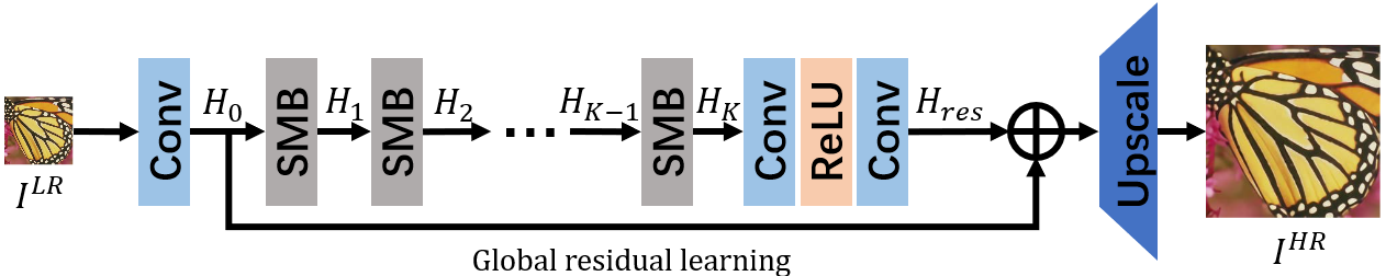
Figure 2. Illustration of the proposed SHSR.

3.1. Network Structure

Fig. 2 shows the entire network design of our SHSR. Firstly, a convolutional layer extracts the features from LR image. The feature space holds more channels than the RGB space and contains more information. The feature extraction can be described as,

(1) $$H_{0}=Conv(I^{LR}),$$

where $I^{LR}$ is the LR instance, and $H_{0}$ is the extracted feature for hierarchical exploration.

After feature extraction, there are SMBs to explore the multi-scale information. The hierarchical features are processed in a progressive manner. For $k$-th SMB, there is,

(2) $$H_{k}=SMB_{k}(H_{k-1}),$$

where $SMB_{k}(\cdot)$ denotes the $k$-th SMB separately. After $K$ SMBs, a padding structure is considered to perform the global residual learning, as,

(3) $$H_{out}=H_{0}+Padding(H_{K}),$$

where $Padding(\cdot)$ denotes the padding structure. The padding structure is composed of two convolutional layers and a ReLU activation.

Finally, HR instance is restored from the explored feature by upscale block, as,

(4) $$I^{HR}=Upscale(H_{out}),$$

where $Upscale(\cdot)$ is the upscale block and composed of two convolutional layers and a sub-pixel convolution.

3.2. Sequential Multi-scale Block

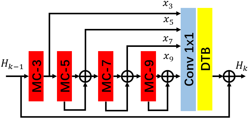
(a) (a) Sequential multi-scale block.

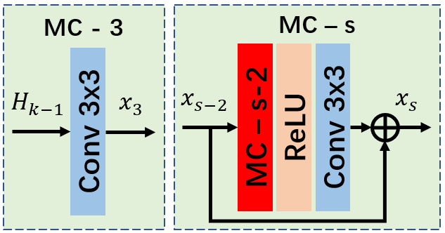
(b) (b) Design of multi-scale exploration combination.

Figure 3. Illustration of proposed sequential multi-scale block (SMB).

Fig. 3 (a) shows the design of proposed SMB. The multi-scale combination with receptive field $s\times s$ (MC-$s$) is designed in a recursive way to explore the hierarchical information. We build the MCs in a sequential way, and derive the larger scale features from smaller ones. Let $x_{s}$ denotes the feature maps with scaling factor $s\times s$, then there are,

(5) $$\left\{\begin{aligned} x_{s}&=MC_{s}(H_{k-1}),&s=3,\\ x_{s}&=MC_{s}(x_{s-2})+x_{s-2},&else.\end{aligned}\right.$$

From Eq. 5, the larger scale features are explored from the former ones, and the sequential exploration can fully consider the inter-scale correlation of features. Instead of directly exploiting the features by filters with different receptive scales, the $MC(\cdot)$ is defined in a recursive way, as shown in Fig. 3 (b). The first $MC_{3}(\cdot)$ is composed of one $3\times 3$ convolutional layer. For other scaling factors, $MC_{s+2}(\cdot)$ is composed of an identical structure of $MC_{s}(\cdot)$, a ReLU activation and a $3\times 3$ convolutional layer. The recursive design is motivated by the linearity of convolution, where a larger kernel can be separated into several smaller filters to keep the receptive field. Different from directly stacking the convolutions, we introduce the ReLU activation for non-linearity into MCs, aiming to build an effective exploration. The residual learning is considered for preserving the original information. It should be noticed that there is no residual connection in $MC_{3}(\cdot)$ since the identical addition is implied by the convolution.

After hierarchical exploration, the different features are concatenated by one $1\times 1$ convolution for information aggregation and one DTB for distribution transmission, as,

(6) $$H_{k}=DTB(Conv([x_{3},...,x_{S}]))+H_{k-1},$$

where $S$ is the largest scaling factor, and $H_{k}$ is the output features of $k$-th SMB. Residual learning aims to preserve the original information.

3.3. Distribution Transformation Block

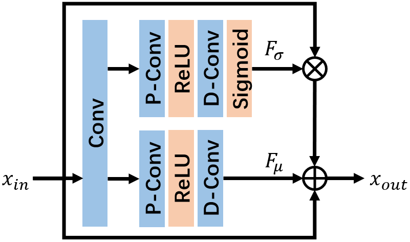
Figure 4. Illustration of the proposed distribution transformation block (DTB). Depth-wise and point-wise convolutions (D-Conv and P-Conv) are designed to explore the spatial and channel-wise correlations separately.

Fig. 4 shows the design of proposed DTB. There is a convolutional layer for input feature $x_{in}$ to exploit the distribution information. After exploitation, depth-wise convolution (D-Conv) and point-wise convolution (P-Conv) are utilized to orthogonally explore the channel-wise and spatial correlations, and ReLU activation is utilized to introduce the non-linearity. The dual paths parallelly learn bias factor $F_{\mu}$ and scaling factor $F_{\sigma}$ separately. Sigmoid activation is specially designed for $F_{\sigma}$ for non-negativity.

The processing step of DTB is formulated as,

(7) $$x_{out}=(x_{in}\otimes F_{\sigma}+F_{\mu})+x_{in},$$

where $x_{in}$, $x_{out}$ denotes the input and output features separately, and $\otimes$ means the element-wise production. The $(x_{in}\otimes F_{\sigma}+F_{\mu})$ in Equation 7 means the described normalization operation of DTB. The shortcut in DTB is designed for improving the gradient transmission and preserving the original information of $x_{in}$ with local residual learning. Local residual learning has been widely considered in SISR works, and has proved to be an effective design for restoration (Lim et al., 2017; Zhang et al., 2018; Zhang et al., 2020a; Liu et al., 2020b).

Eq. 7 holds an advanced formulation than attention-based methods, which regard the bias factor $F_{\mu}$ as zero. Similar to normalization methods, DTB jointly utilizes bias and scaling factors to adjust the features. Traditional normalization blocks, such as batch normalization (Ioffe and Szegedy, 2015) (BN), usually constrainedly adjust the feature into some standard distribution. However, this kind of adjustment may not be suitable for SISR problem which gets rid of range flexibility from networks (Lim et al., 2017). DTB provides the similar formulation to perform the adjustment and removes the statistical estimation step. With the learned parameters, DTB transforms the feature distribution for better SISR performance.

3.4. Implementation Details

In SHSR, all convolutional layers are with kernel size as $3\times 3$ except for the mentioned $1\times 1$ concatenation in SMB. The filter number of convolutional layers in SMBs and DTBs is set as $c=64$ while the upscale block contains $c_{0}=3\times u^{2}$ filters, where $u$ denotes the up-sampling factor for HR image. The upscale block contains a convolutional layer with $64$ filters, and a rescaling tail that follows a similar structure as MSRN (Li et al., 2018), which is composed of one convolution layer and one sub-pixel convolution. There are $K=8$ SMBs stacked in SHSR, and the maximum scaling factor in SMB is set as $S=9$.

4. Discussion

Difference to MSRN (Li et al., 2018)

MSRN introduced a multi-scale block termed as MSRB with $3\times 3$ and $5\times 5$ convolutional layers. In MSRB, features from two kinds of convoluitonal layers are crossly concatenated and explored, and an $1\times 1$ convolutional layer is utilized to fuse the multi-scale features. Different from MSRB, there are features from four different scales extracted by SMB, and concatenated with one convolutional layer for fusion. Features from different scales are explored sequentially, and residual connections are utilized for information preservation. Multi-scale information is extracted by layers with different kernel sizes in MSRB, while SMB designs the multi-scale structure in a recursive way, which focuses on the inter-scale correlations and decreases the network parameters. Features from different MSRBs are collected and concatenated with a convolutional layer for global feature fusion, while blocks in SHSR are stacked with global residual learning. Besides multi-scale design, a novel distribution transformation mechanism DTB is designed in SHSR. With the elaborated design, SHSR achieves better PSNR/SSIM results on all testing benchmarks than MSRN with fewer parameters and lower computation complexity.

SMB is designed based on the observation that larger scale information can derive from the smaller features. As such, the explored smaller features are helpful for effective larger scale exploration. Different from SMB, MSRN considers the hierarchical exploration in a parallel design, and utilizes the filters with different receptive fields to process the features. On one hand, the parallel design is not efficient for hierarchical exploration since it does not consider the relationship among hierarchical features. On the other hand, using filters with different receptive fields is not an efficient way to process the multi-scale information. According to the principle of convolution, the larger filter can be equivalently decomposed into a sequence of smaller filters with fewer parameters and lower computational complexity (Szegedy et al., 2015). As such, our network achieves better PSNR/SSIM performance than MSRN with much fewer parameters and lower MACs. Compared with MSRN, our network achieves 0.1 dB PSNR higher on Urban100 and 0.2 dB higher on Manga109 with scaling factor $\times 4$, while our network only holds near 56% parameters and MACs.

Difference to Channel-wise Attention (Hu et al., 2020b)

There is an effective channel-wise attention design in SENet, which has been widely utilized for different image restoration problems. In channel-wise attentions, information from different channels is evaluated by global average pooling. Two full connection layers with a ReLU activation are designed to explore the attentions, and a Sigmoid activation is introduced for non-negativity.

DTB aims to learn both the channel-wise and spatial attention for image SR. There is global average pooling in vanilla channel-wise attention methods, which does not consider the spatial diversity of different feature maps. The output of channel-wise attention is a vector for weighting the feature maps, and the pixels on the same feature map share the same weight. Different from channel-wise attention, DTB considers the distribution transformation with both scaling and bias factors. The operation of DTB follows a similar formulation to the normalization manner. The D-Conv and P-Conv in DTB orthogonally explore the feature maps, and calculate the bias and scaling factors with the same shape of input features. In other words, every pixel on the feature maps will get different weights and offsets. The normalization manner and the diversity of factors make the DTB performs better than vanilla channel-wise attention. According to the ablation study, DTB achieves 0.03 dB PSNR higher than channel-wise attention on different benchmarks with scaling factor $\times 4$.

Difference to MS-LapSRN (Lai et al., 2019)

MS-LapSRN is a progressive network for image super-resolution. In MS-LapSRN, the progressive structure is designed for images restorations with multiple resolutions by using one network. Residual maps are learned from the network sequentially with the increase of resolutions. In SHSR, an end-to-end network is proposed for image super-resolution with a specific up-sampling factor. The multi-scale structure is mainly designed in SMB to extract the hierarchical information. Information from multi-scale features is sequentially extracted to concentrate on the inter-scale correlations. By utilizing the sequential exploration and building a deeper network, SHSR achieves better performance than MS-LapSRN.

MS-LapSRN builds the network following the Laplacian Pyramid architecture, and progressively enlarges the feature’s resolution for multi-scale restoration. The blocks in MS-LapSRN are simply designed by stacking the convolutional and ReLU layers. To boost the restoration performance, MS-LapSRN shares the parameters of different components and restore the image in a recursive way. Different from MS-LapSRN, SMB considers the multi-scale exploration by designing the blocks with different receptive fields, rather than simply enlarging the feature map. We argue that enlarging the feature map will increase the computational cost. As such, our network achieves near 1 dB PSNR higher than MS-LapSRN with scaling factor $\times 4$.

Difference to Recent Hierarchical Designs

Recently, there are multi-scale designs for effective image SR. HDRN (Jiang et al., 2020) and HRAN (Behjati et al., 2020) are two representative hierarchical networks. The proposed sequential multi-scale block (SMB) in our network enjoys a different motivation and design from HDRN and HRAN for more effective hierarchical exploration.

HDRN stacks the convolutional layers with the same receptive field, and densely connects the features to consider the hierarchy. The dense connection in HDRN directly mixtures the explored features from all scales, which does not explicitly consider the correlation of multi-scale information. Different from HDRN, we observe that the larger scale information can derive from the smaller scale features, and design the sequential feature exploration in SMB for effective hierarchical processing. Based on the sequential design, our network achieves near 0.3 dB PSNR higher than HDRN with scaling factor $\times 4$.

Similar to HDRN, HRAN considers the hierarchical exploration by concatenating the explored features from different blocks with $1\times 1$ convolution. The blocks in HRAN enjoy the same network design and receptive field, and do not consider the hierarchical correlations. In our SMB, the hierarchical exploration is considered in a sequential manner, which follows the observation of the multi-scale correlation. The blocks in SMB hold different receptive fields and progressively explore the features. According to the report of HRAN (Behjati et al., 2020), there is around 0.06 dB PSNR benefit from its hierarchical exploration. In our network, the multi-scale design in SMB provides near 0.3 dB PSNR improvement in Table 1.

5. Experiments

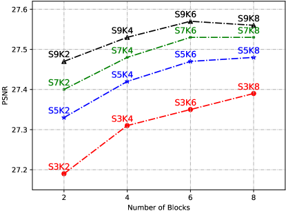
Figure 5. Investigation on different $S$ and $K$ with scaling factor $\times 4$.

5.1. Settings

The proposed SHSR is trained with DIV2K (Agustsson and Timofte, 2017) dataset. DIV2K is a high-quality dataset with 2K resolution images from real world. There are 800 training images, 100 validation images and 100 test images in DIV2K dataset. In this paper, 800 images are chosen for training and 5 images for validation. For testing, five benchmarks widely used in image super-resolution works: Set5 (Bevilacqua et al., 2012), Set14 (Zeyde et al., 2010), B100 (Martin et al., 2001), Urban100 (Huang et al., 2015), and Manga109 (Matsui et al., 2017) are chosen. We train our SHSR with PyTorch (Paszke et al., 2019) on NVIDIA GTX-1080Ti GPU. The training images are randomly flipped and rotated for data augmentation. Patch size of LR image for training is set as $48\times 48$. SHSR are trained for 1000 iterations with $\ell_{1}$ loss, and the parameters are updated with an Adam (Kingma and Ba, 2014) optimizer. The learning rate of optimizer is chosen as $lr=10^{-4}$, and halved for every 200 iterations. The degradation model is chosen as bicubic down (BI) with scaling factor $\times 2$, $\times 3$, and $\times 4$. PSNR and SSIM are chosen as the indicators for quantitative comparison with other works. Self-ensemble strategy is used to improve the performance, and the extension model is termed as as SHSR⁺.

5.2. Model Analysis

5.2.1. Analysis on Network Settings

In SHSR, the largest scale of SMB is set as $S=9$ and the number of SMB is chosen as $K=8$. To show the effect of $S$ and $K$, models are trained with different scales and block numbers for 200 epochs. Quantitative comparisons are made on B100 with scaling factor $\times 4$. The visualization results are shown in Fig. 5. From Fig. 5, both $S$ and $K$ can affect the network performance. In general, with the increase of $S$ and $K$, the network achieves better results. Compared with $K$, $S$ counts more for the performance. On one hand, when $S$ is larger, the network is deeper. On the other hand, with the increase of $S$, features from more scales are considered.

5.2.2. Analysis on SMB

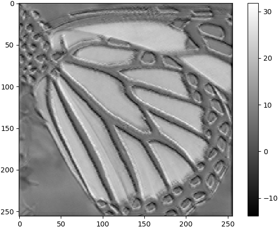
(a) (a)

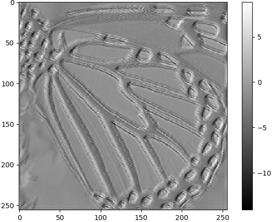
(b) (b)

(c) (c)

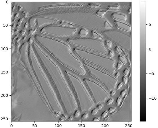
(d) (d)

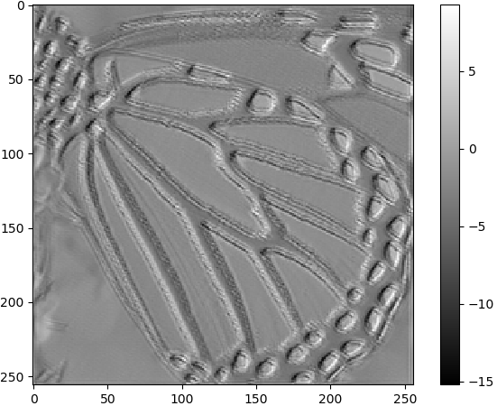
(e) (e)

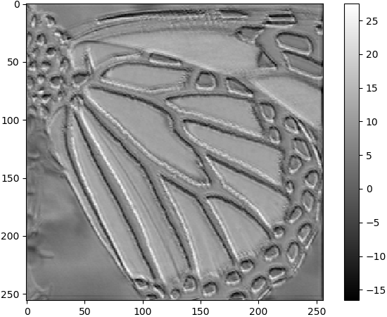
(f) (f)

Figure 6. Illustrations of multi-scale features. (a) and (f) denote the input and output features. (b)-(e) denote the features with scaling factor 3, 5, 7, and 9.

Table 1. PSNR/SSIM results of multi-scale mechanism in SMB with scaling factor $\times 4$.

Multi	Set5	Set14	B100	Urban100
w	32.34/0.8971	28.71/0.7850	27.66/0.7392	26.37/0.7953
w/o	32.03/0.8932	28.51/0.7799	27.53/0.7348	25.90/0.7803

There is multi-scale design in SMB extracting the hierarchical information. To show the performance of multi-scale design, comparisons are conducted without different combinations of convolutional layers. All combinations are replaced by only one $3\times 3$ convolutional layer. In other words, all the scales in SMB are identical to $3\times 3$. The results are shown in Table. 1 on four benchmarks with scaling factor $\times 4$. From Table 1, model with multi-scale design achieves better PSNR/SSIM results than the other one. There are two reasons for the performance improvement. On one hand, the features of different scales contain more information, which helps to recover the complex structural textures. On the other hand, the multi-scale structures are built in a recursive way. With the combination of convolutional layers, the depth of SHSR is increased, which may be helpful to improve the network representation.

Furthermore, we analyze the exploited features from different scales, which are shown in Fig. 6. The multi-scale features are exploited from different layer combinations. With the increasing of scale factors, the structural information becomes sharper and clearer, and the tiny textures become flat. This accords with the notion that multi-scale features contain different information.

In SMB, residual connections are introduced to preserve the information from small scales. Feature fusion with $1\times 1$ convolution is also used to concatenate information from different scales. To show the performance of information preservation and feature fusion, we perform the comparisons without residual and $1\times 1$ convolution. The results are shown in Table. 2, where Res and Fuse denote the residual connection and concatenation separately. Three benchmarks covering different kinds of textures are used for testing with scaling factor $\times 4$. From the Table 2, residual and feature fusion are both efficient for different benchmarks. For Set5, residual structure performs better than fusion, achieving around 0.1dB improvement. For B100 and Urban100, feature fusion can recover the texture more effectively. Set5 contains less high-frequency information than the other benchmarks, while B100 and Urban100 are composed of abundant images from real world. From this perspective, residual connection is suitable for simple images, while feature fusion performs better on complex structural textures.

Table 2. PSNR/SSIM results of different structures in SMB with scaling factor $\times 4$.

Res	Fuse	Set5	B100	Urban100
w	w	32.34/0.8971	27.66/0.7392	26.37/0.7953
w	w/o	32.35/0.8971	27.64/0.7384	26.34/0.7942
w/o	w	32.24/0.8963	27.65/0.7388	26.36/0.7955

5.2.3. Analysis on Multi-scale Combination.

In SHSR, recursive layer combinations (MCs) are proposed to substitute convolutional layers with different kernel sizes. To show the performance of substitution, PSNR/SSIM comparisons are made on five benchmarks with scaling factor $\times 4$. To ensure the same receptive field, network without combinations is built with layers holding the kernel sizes as $5\times 5$, $7\times 7$ and $9\times 9$ separately. The results are shown in Table 3. From Table 3, model built with layer combinations achieves better PSNR/SSIM results on all five testing benchmarks, showing the performance of recursive design. Meanwhile, there are around 40.2% off on parameters and MACs when utilizing recursive combinations.

Table 3. PSNR/SSIM results, parameters, and MACs of recursive combination in SMB with scaling factor $\times 4$.

Comb	Param	MACs	Set5	Set14	B100	Urban100	Manga109
w	3,598K	207.2G	32.34/0.8971	28.71/0.7850	27.66/0.7392	26.37/0.7953	30.71/0.9107
w/o	6,020K	346.7G	32.07/0.8932	28.53/0.7804	27.53/0.7350	25.93/0.7819	30.16/0.9043

5.2.4. Analysis on Distribution Transformation.

In SHSR, DTB is investigated for distribution transformation. To show the performance of proposed DTB, comparisons are designed on three testing benchmarks. We compare the models with DTB, channel-wise attention (CA) (Hu et al., 2020b), and no transformation. The results are shown in Table 4. From the table, the model with DTB achieves the best performance on all testing benchmarks. The model with channel-wise attentions achieves better PSNR/SSIM results than that without attentions. The results demonstrate that distribution transformation is efficient for image super-resolution.

Table 4. PSNR/SSIM results of different transformations with scaling factor $\times 4$.

Method	Set5	Set14	Urban100
DTB	32.34/0.8971	28.71/0.7850	26.37/0.7953
CA (Hu et al., 2020b)	32.31/0.8968	28.69/0.7844	26.34/0.7940
w/o	32.29/0.8965	28.68/0.7851	26.29/0.7940

To analyze the operation of DTB, factors $F_{\gamma}$, $F_{\beta}$ and the feature maps before and after attention are visualized in Fig. 7. From the illustrations, learned attentions are more concentrated on structural textures. $F_{\gamma}$ and $F_{\beta}$ vary sharply on the area of edges and complex textures. After attentions, the features are more discriminative on structural textures, which is a convincing evidence of that the transformation mechanism concentrates more on the important high-frequency information.

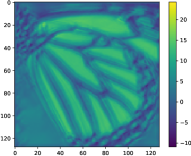
(a) (a) Feature before DTB

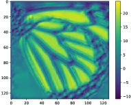
(b) (b) Feature after DTB

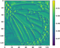
(c) (c) $F_{\sigma}$ from DTB

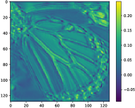
(d) (d) $F_{\mu}$ from DTB

Figure 7. Visualization feature maps of DTB.

5.3. Comparison with State-of-the-Arts

Table 5. Average PSNR/SSIM, parameters and MACs results with degradation model BI $\times 2$, $\times 3$, and $\times 4$ on five benchmarks. The best and second performances are shown in bold and underline.

Scale	Model	Params	MACs	Set5 (Bevilacqua et al., 2012)	Set14 (Zeyde et al., 2010)	B100 (Martin et al., 2001)	Urban100 (Huang et al., 2015)	Manga109 (Matsui et al., 2017)
				PSNR/SSIM	PSNR/SSIM	PSNR/SSIM	PSNR/SSIM	PSNR/SSIM
$\times 2$	SRCNN (Dong et al., 2016)	57K	52.7G	36.66/0.9542	32.42/0.9063	31.36/0.8879	29.50/0.8946	35.74/0.9661
	FSRCNN (Dong et al., 2016)	12K	6.0G	37.00/0.9558	32.63/0.9088	31.53/0.8920	29.88/0.9020	36.67/0.9694
	VDSR (Kim et al., 2016a)	665K	612.6G	37.53/0.9587	33.03/0.9124	31.90/0.8960	30.76/0.9140	37.22/0.9729
	DRCN (Kim et al., 2016b)	1,774K	17,974.3G	37.63/0.9588	33.04/0.9118	31.85/0.8942	30.75/0.9133	37.63/0.9723
	CNF (Ren et al., 2017)	337K	311.0G	37.66/0.9590	33.38/0.9136	31.91/0.8962	-	-
	LapSRN (Lai et al., 2017)	813K	29.9G	37.52/0.9590	33.08/0.9130	31.80/0.8950	30.41/0.9100	37.27/0.9740
	DRRN (Tai et al., 2017)	297K	6,796.9G	37.74/0.9591	33.23/0.9136	32.05/0.8973	31.23/0.9188	37.92/0.9760
	BTSRN (Fan et al., 2017)	410K	207.7G	37.75/-	33.20/-	32.05/-	31.63/-	-
	MemNet (Tai et al., 2017)	677K	2,662.4G	37.78/0.9597	33.28/0.9142	32.08/0.8978	31.31/0.9195	37.72/0.9740
	SelNet (Choi and Kim, 2017)	974K	225.7G	37.89/0.9598	33.61/0.9160	32.08/0.8984	-	-
	CARN (Ahn et al., 2018)	1,592K	222.8G	37.76/0.9590	33.52/0.9166	32.09/0.8978	31.92/0.9256	38.36/0.9765
	MSRN (Li et al., 2018)	5,930K	1367.5G	38.08/0.9607	33.70/0.9186	32.23/0.9002	32.29/0.9303	38.69/0.9772
	PRLSR (Liu et al., 2020a)	1,363K	187.3G	38.09/0.9608	33.69/.09191	32.25/0.9005	32.35/0.9308	-
	OISR-RK2 (He et al., 2019)	4,970K	1145.7G	38.12/0.9609	33.80/0.9193	32.26/0.9006	32.48/0.9317	-
	LMAN-s (Wan et al., 2020)	1,531K	91.7G	37.94/0.9603	33.49/0.9167	32.08/0.8984	31.85/0.9251	38.43/0.9765
	SHSR	3,577K	824.2G	38.13/0.9609	33.85/0.9204	32.28/0.9010	32.59/0.9328	38.91/0.9775
	EDSR (Lim et al., 2017)	40,729K	9,388.8G	38.11/0.9602	33.92/0.9195	32.32/0.9013	32.93/0.9351	39.10/0.9773
	D-DBPN (Haris et al., 2020)	5,953K	3,746.2G	38.09/0.9600	33.85/0.9190	32.27/0.9000	32.55/0.9324	38.89/0.9775
	SRFBN (Li et al., 2019)	2,140K	5,043.5G	38.11/0.9609	33.82/0.9196	32.29/0.9010	32.62/0.9328	39.08/0.9779
	SHSR+	3,577K	6,593.6G	38.22/0.9612	33.90/0.9205	32.34/0.9015	32.78/0.9342	39.15/0.9781
$\times 3$	SRCNN (Dong et al., 2016)	57K	52.7G	32.75/0.9090	29.28/0.8209	28.41/0.7863	26.24/0.7989	30.59/0.9107
	FSRCNN (Dong et al., 2016)	12K	5.0G	33.16/0.9140	29.43/0.8242	28.53/0.7910	26.43/0.8080	30.98/0.9212
	VDSR (Kim et al., 2016a)	665K	612.6G	33.66/0.9213	29.77/0.8314	28.82/0.7976	27.14/0.8279	32.01/0.9310
	DRCN (Kim et al., 2016b)	1,774K	17,974.3G	33.82/0.9226	29.76/0.8311	28.80/0.7963	27.15/0.8276	32.31/0.9328
	CNF (Ren et al., 2017)	337K	311.0G	33.74/0.9226	29.90/0.8322	28.82/0.7980	-	-
	DRRN (Tai et al., 2017)	297K	6,796.9G	34.03/0.9244	29.96/0.8349	28.95/0.8004	27.53/0.8378	32.74/0.9390
	BTSRN (Fan et al., 2017)	410K	176.2G	34.03/-	29.90/-	28.97/-	27.75/-	-
	MemNet (Tai et al., 2017)	677K	2,662.4G	34.09/0.9248	30.00/0.8350	28.96/0.8001	27.56/0.8376	32.51/0.9369
	SelNet (Choi and Kim, 2017)	1,159K	120.0G	34.27/0.9257	30.30/0.8399	28.97/0.8025	-	-
	CARN (Ahn et al., 2018)	1,592K	118.8G	34.29/0.9255	30.29/0.8407	29.06/0.8034	28.06/0.8493	33.49/0.9440
	MSRN (Li et al., 2018)	6,114K	626.6G	34.46/0.9278	30.41/0.8437	29.15/0.8064	28.33/0.8561	33.67/0.9456
	OISR-RK2 (He et al., 2019)	5,640K	578.6G	34.55/0.9282	30.46/0.8443	29.18/0.8075	28.50/0.8597	-
	PRLSR (Liu et al., 2020a)	1,456K	94.5G	34.47/0.9278	30.43/0.8436	29.14/0.8060	28.27/0.8541	-
	SHSR	3,586K	366.6G	34.57/0.9284	30.43/0.8444	29.19/0.8075	28.51/0.8601	33.85/0.9465
	EDSR (Lim et al., 2017)	43,680K	4,471.5G	34.65/0.9280	30.52/0.8462	29.25/0.8093	28.80/0.8653	34.17/0.9476
	SRFBN (Li et al., 2019)	2,832K	6,023.8G	34.70/0.9292	30.51/0.8461	29.24/0.8084	28.73/0.8641	34.18/0.9481
	SHSR+	3,586K	2,932.8G	34.65/0.9289	30.54/0.8461	29.24/0.8087	28.71/0.8630	34.10/0.9480
$\times 4$	SRCNN (Dong et al., 2016)	57K	52.7G	30.48/0.8628	27.49/0.7503	26.90/0.7101	24.52/0.7221	27.66/0.8505
	FSRCNN (Dong et al., 2016)	12K	4.6G	30.71/0.8657	27.59/0.7535	26.98/0.7150	24.62/0.7280	27.90/0.8517
	VDSR (Kim et al., 2016a)	665K	612.6G	31.35/0.8838	28.01/0.7674	27.29/0.7251	25.18/0.7524	28.83/0.8809
	DRCN (Kim et al., 2016b)	1,774K	17,974.3G	31.53/0.8854	28.02/0.7670	27.23/0.7233	25.14/0.7510	28.98/0.8816
	CNF (Ren et al., 2017)	337K	311.0G	31.55/0.8856	28.15/0.7680	27.32/0.7253	-	-
	LapSRN (Lai et al., 2017)	813K	149.4G	31.54/0.8850	28.19/0.7720	27.32/0.7280	25.21/0.7560	29.09/0.8845
	DRRN (Tai et al., 2017)	297K	6,796.9G	31.68/0.8888	28.21/0.7720	27.38/0.7284	25.44/0.7638	29.46/0.8960
	BTSRN (Fan et al., 2017)	410K	207.7G	31.85/-	28.20/-	27.47/-	25.74/-	-
	MemNet (Tai et al., 2017)	677K	2,662.4G	31.74/0.8893	28.26/0.7723	27.40/0.7281	25.50/0.7630	29.42/0.8942
	SelNet (Choi and Kim, 2017)	1,417K	83.1G	32.00/0.8931	28.49/0.7783	27.44/0.7325	-	-
	CARN (Ahn et al., 2018)	1,592K	90.9G	32.13/0.8937	28.60/0.7806	27.58/0.7349	26.07/0.7837	30.40/0.9082
	MSRN (Li et al., 2018)	6,373K	368.6G	32.26/0.8960	28.63/0.7836	27.61/0.7380	26.22/0.7911	30.57/0.9103
	s-LWSR64 (Li et al., 2020b)	2,277K	131.1G	32.28/0.8960	28.34/0.7800	27.61/0.7380	26.19/0.8910	-
	OISR-RK2 (He et al., 2019)	5,500K	412.2G	32.32/0.8965	28.72/0.7843	27.66/0.7390	26.37/0.7953	-
	PRLSR (Liu et al., 2020a)	1,437K	66.9G	32.31/0.8962	28.71/0.7838	27.64/0.7378	26.22/0.7892	-
	SHSR	3,598K	207.2G	32.34/0.8971	28.71/0.7850	27.66/0.7392	26.37/0.7953	30.71/0.9107
	EDSR (Lim et al., 2017)	43,089K	2,895.8G	32.46/0.8968	28.80/0.7876	27.71/0.7420	26.64/0.8033	31.02/0.9148
	D-DBPN (Haris et al., 2020)	10,426K	5,213.0G	32.47/0.8980	28.82/0.7860	27.72/0.7400	26.38/0.7946	30.91/0.9137
	SRFBN (Li et al., 2019)	3,631K	7,466.1G	32.47/0.8983	28.81/0.7868	27.72/0.7409	26.60/0.8015	31.15/0.9160
	SHSR+	3,598K	1,657.6G	32.47/0.8984	28.81/0.7870	27.72/0.7405	26.55/0.7995	31.07/0.9144

To make quantitive comparison, we compare the PSNR/SSIM results with several small works: SRCNN (Dong et al., 2016), FSRCNN (Dong et al., 2016), VDSR (Kim et al., 2016a), DRCN (Kim et al., 2016b), CNF (Ren et al., 2017), LapSRN (Lai et al., 2017), DRRN (Tai et al., 2017), BTSRN (Fan et al., 2017), MemNet (Tai et al., 2017), SelNet (Choi and Kim, 2017), CARN (Ahn et al., 2018), MSRN (Li et al., 2018), s-LWSR (Li et al., 2020b), PRLSR (Liu et al., 2020a), LMAN-s (Wan et al., 2020) and OISR (He et al., 2019). For a fair comparison, extension model SHSR⁺ with self-ensemble is compared with large networks: EDSR (Lim et al., 2017), D-DBPN (Haris et al., 2020), and SRFBN (Li et al., 2019).

Table 5 shows the PSNR/SSIM comparisons among several methods. From the results, SHSR achieves competitive or better performance than other small works on all five benchmarks. Compared with the multi-scale method MSRN, SHSR gains 0.3dB increase on Urban100 with $\textbf{BI}\times 2$ degradation. Furthermore, SHSR achieves competitive or better performance than OISR with around 34% parameters off. Notice that SHSR achieves the best performances on B100, Urban100, and Manga109 with all degradation models. The three benchmarks contain plentiful structural information and edges, which consist of comic covers and real world photos. From this point of view, SHSR can recover the high-frequency information more effectively than others.

Meanwhile, we compare the computation complexity and parameters with other works. Computation complexity is modeled as the number of multiply-accumulate operations (MACs). Since it is an implementation independent factor, MACs can purely describe the computation complexity from the mathematical perspective. Comparisons of MACs are conducted by producing a 720P ($1280\times 720$) resolution image from corresponding LR image with different scaling factors. The MACs of SHSR is calculated by PyTorch-OpCounter  and multiplied by 8 for SHSR⁺.

From the results, SHSR achieves competitive or better PSNR/SSIM results than others with fewer parameters and MACs, which proves to be the efficient design. Compared with OISR, SHSR holds near half MACs and parameters with competitive or better PSNR/SSIM performances with $\textbf{BI}\times 4$ degradation. Compared with larger networks, SHSR⁺ achieves competitive performances with much fewer MACs and parameters. Specially, SHSR⁺ holds near half of the MACs and one tenth of the parameters than EDSR with $\textbf{BI}\times 4$ degradation, and achieves superior PSNR results on Set5, Set14, B100, and Manga109 datasets.

To further investigate the effectiveness of SHSR, we compare our network with recent state-of-the-art deep SISR networks. Table 6 shows the PSNR, parameters and MACs comparison with scaling factor $\times 4$. In the table, we mainly compare our network with recent state-of-the-art SISR works (RCAN (Zhang et al., 2018), MSRN (Li et al., 2018), USRNet (Zhang et al., 2020a), DRN (Guo et al., 2020), SRFBN (Li et al., 2019), EBRN (Qiu et al., 2019), OISR-RK2 (He et al., 2019)). Our network holds near 20% parameters and 22% MACs than RCAN with only less than 0.5 dB PSNR degradation. Specifically, we only drop less than 0.2 dB PNSR on Set14 and B100, which is marginal for visual quality. When compared with other state-of-the-art works, our network also achieves competitive performance with much fewer parameters and MACs. There is only less than 0.2 dB PSNR drop for our network when compared with SRFBN (Li et al., 2019), while we save near 97.2% MACs. For DRN (Guo et al., 2020), we save near 73% parameters and 85% MACs with less than 0.4 dB PSNR drop. When compared with EBRN (Qiu et al., 2019), our network saves near 70% parameters and 97% MACs and drops less than 0.4 dB on PSNR. MSRN (Li et al., 2018) and OISR-RK2 (He et al., 2019) are two recent works with similar parameters and MACs to our network. Compared with OISR, our network achieves competitive performance and saves near 34% parameters and 50% MACs. Our network also achieves better PSNR results than MSRN with fewer parameters and MACs.

Table 6. PSNR, parameters and MACs comparisons with state-of-the-art SISR works with scaling factor $\times 4$.

Method	RCAN (Zhang et al., 2018)	USRNet (Zhang et al., 2020a)	DRN (Guo et al., 2020)	MSRN (Li et al., 2018)	SRFBN (Li et al., 2019)	EBRN (Qiu et al., 2019)	OISR-RK2 (He et al., 2019)	Ours
Params (K)	17410	17016	9825	6373	3630	11279	5500	3598
MACs (G)	919.1	8545.8	1406.3	368.6	7466.1	6439.0	412.2	207.2
Set5	32.63	32.42	32.74	32.26	32.47	32.79	32.32	32.34
Set14	28.87	28.83	28.98	28.63	28.81	29.01	28.72	28.71
B100	27.77	27.69	27.83	27.61	27.72	27.85	27.66	27.66

For better illustrating the performance, we plot the PSNR, MACs and parameter comparisons on B100 benchmark with BI$\times 4$ degradation. Figure 8 and 9 show the comparison. From the results, our network makes a good trade-off on model complexity and performance.

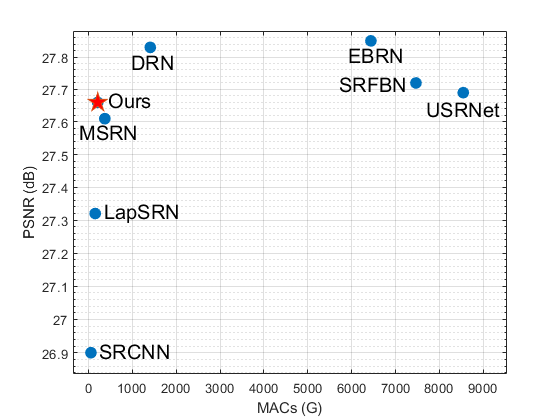
Figure 8. Visualization comparisons on PSNR and MACs with scaling factor $\times 4$.

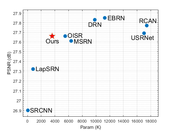
Figure 9. Visualization comparisons on PSNR and parameters with scaling factor $\times 4$.

Besides quantitative comparisons, we also analyze the qualitative restoration performance via visualization comparisons. Three images from Urban100 benchmark are chosen for comparison with BI $\times 4$ degradation, which is shown in Fig. 10. These images are from real world with abundant high-frequency textures and competitive for restoration with large scaling factors. From the result, SHSR can recover the structural information effectively, and find more accurate textures than other works.

Besides Urban100, we also conduct the experiments on Manga109, which is composed of comic book covers with plentiful line structures. The result is shown in Fig. 11. From the visualization comparison, SHSR recovers more lines and structural textures.

Since Manga109 is a normal textured benchmark, we also compare the methods in the very textured situation, which is shown in Fig. 12. The feather contains plentiful small lines and textures which are hard for recovery. From the comparison, SHSR can restore the textured image more accurately than MSRN.

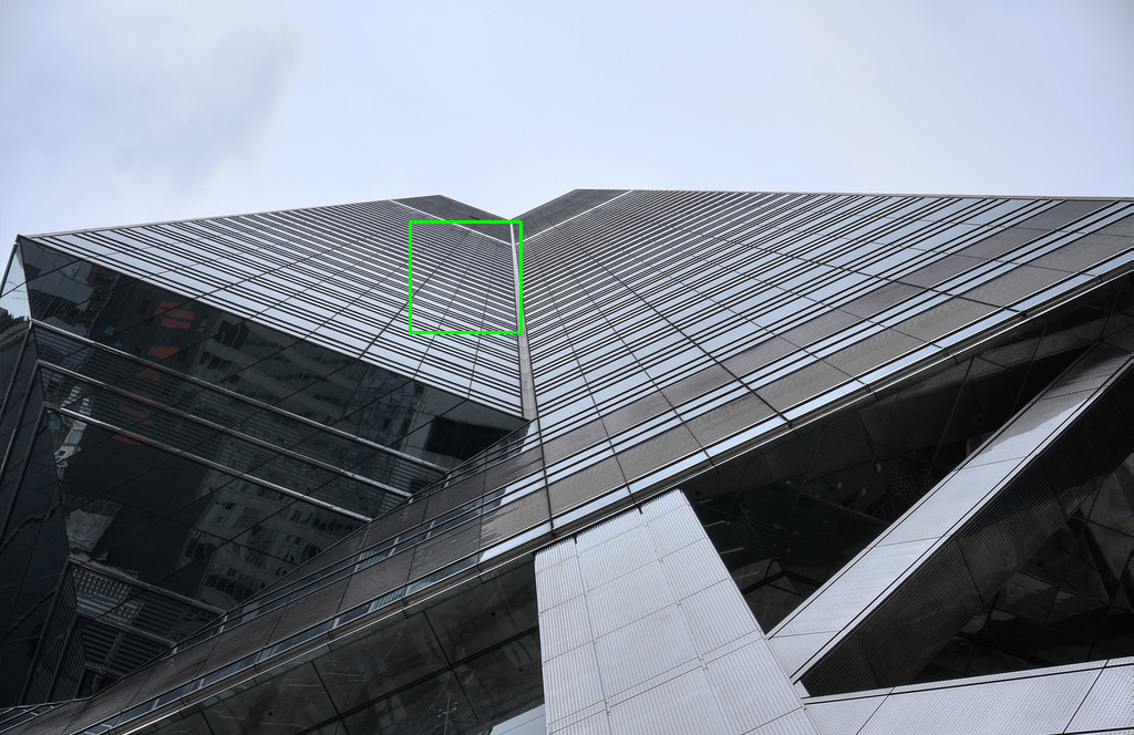
(a) image_059 from Urban100

(b) HR (PSNR/SSIM)

(c) LR (18.96/0.7246)

(d) Bicubic (19.21/0.7331)

(e) VDSR (Kim et al., 2016a) (19.94/0.7910)

(f) MSLapSRN (Lai et al., 2019) (19.92/0.7894)

(g) CARN (Ahn et al., 2018) (20.82/0.8234)

(h) MSRN (Li et al., 2018) (21.11/0.8369)

(i) Ours (21.44/0.8447)

(j) image_067 from Urban100

(k) HR (PSNR/SSIM)

(l) LR (14.95/0.7116)

(m) Bicubic (15.80/0.7490)

(n) VDSR (Kim et al., 2016a) (17.30/0.8474)

(o) MSLapSRN (Lai et al., 2019) (17.34/0.8577)

(p) CARN (Ahn et al., 2018) (18.12/0.8882)

(q) MSRN (Li et al., 2018) (18.58/0.8950)

(r) Ours (18.84/0.9035)

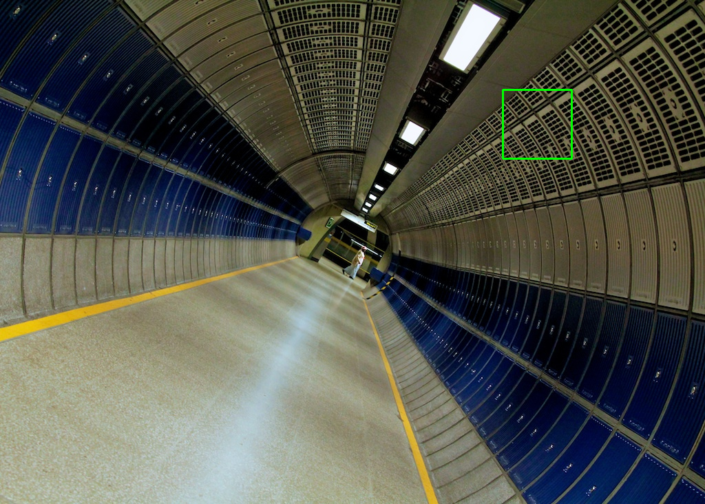
(s) image_078 from Urban100

(t) HR (PSNR/SSIM)

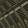
(u) LR (23.74/0.7624)

(v) Bicubic (24.49/0.7866)

(w) VDSR (Kim et al., 2016a) (25.49/0.8401)

(x) MSLapSRN (Lai et al., 2019) (25.41/0.8395)

(y) CARN (Ahn et al., 2018) (25.88/0.8536)

(z) MSRN (Li et al., 2018) (26.12/0.8598)

(aa) Ours (26.45/0.8658)

Figure 10. Visualization comparisons on Urban100 with BI $\times 4$ degradation.

(a) HR (PSNR/SSIM)

(b) LR (20.16/0.8521)

(c) MSRN (Li et al., 2018) (26.31/0.9296)

(d) SHSR (26.46/0.9637)

(e) HR (PSNR/SSIM)

(f) LR (21.34/0.8693)

(g) MSRN (Li et al., 2018) (27.49/0.9690)

(h) SHSR (27.76/0.9637)

Figure 11. Visualization comparisons on Manga109 with BI $\times 4$ degradation.

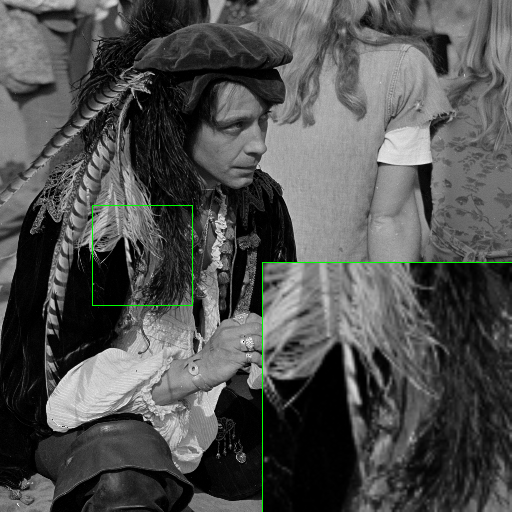
(a) HR (PSNR/SSIM)

(b) LR (23.92/0.6380)

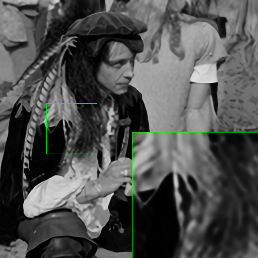
(c) MSRN (Li et al., 2018) (26.11/0.7529)

(d) SHSR (26.18/0.7547)

Figure 12. Visualization comparisons on Set14 with BI $\times 4$ degradation.

To make the comparison more convincing, we compare the visualization performance on different objects, such as plant, grass and animals. Figure 13 shows the visual results and PSNR results compared with EDSR, D-DBPN and SRFBN on BSD100 benchmark with various objects. It should be noted that EDSR, D-DBPN, and SRFBN are heavy networks and hold much more parameters and MACs than our network. Even though, our network can also achieve competitive or better visualization or objective performance than these works.

(a) HR (PSNR)

(b) EDSR (25.92)

(c) DBPN (25.97)

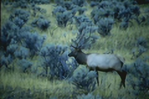
(d) SRFBN (25.95)

(e) Ours (25.94)

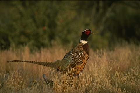
(f) HR (PSNR)

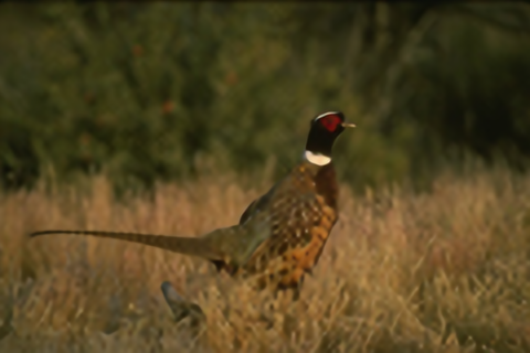
(g) EDSR (28.59)

(h) DBPN (28.63)

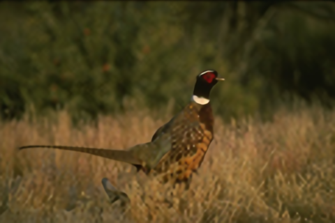
(i) SRFBN (28.61)

(j) Ours (28.60)

(k) HR (PSNR)

(l) EDSR (30.63)

(m) DBPN (30.66)

(n) SRFBN (30.68)

(o) Ours (30.69)

(p) HR (PSNR)

(q) EDSR (27.21)

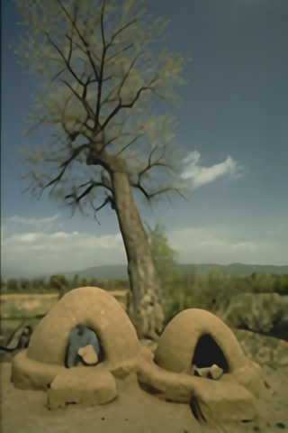
(r) DBPN (27.37)

(s) SRFBN (27.32)

(t) Ours (27.30)

Figure 13. Visualization comparisons on BSD100 benchmark with BI $\times 4$ degradation.

Furthermore, we investigate the restoration capacity on blurred images. From the definition of SISR problem, these works can naturally handle the blurry issue which is regarded as a low-pass filter. We compare the proposed SHSR with recent works with blur and $\times 3$ down-sampling (BD$\times 3$) degradation, which is shown in Tab. 7. From the comparison, SHSR achieves competitive PSNR/SSIM performance with RDN, and the extension model SHSR⁺ achieves superior performance than all other works. It should be noted that RDN holds 22,308K parameters and 2,282.2G MACs, which are much more than SHSR. From this perspective, SHSR is an efficient design which can effectively restore the blurred images.

Table 7. PSNR/SSIM results with BD$\times 3$ degradation.

Method	Bicubic	SRCNN (Dong et al., 2016)	VDSR (Kim et al., 2016a)	IRCNN_G (Zhang et al., 2017)	IRCNN_C (Zhang et al., 2017)	RDN (Zhang et al., 2020a)	SHSR	SHSR+
Set5	28.78/0.8308	32.05/0.8944	33.25/0.9150	33.38/0.9182	33.17/0.9157	34.58/0.9280	34.53/0.9274	34.66/0.9284
Set14	26.38/0.7271	28.80/0.8074	29.46/0.8244	29.63/0.8281	29.55/0.8271	30.53/0.8447	30.51/0.8442	30.60/0.8453
B100	26.33/0.6918	28.13/0.7736	28.57/0.7893	28.65/0.7922	28.49/0.7886	29.23/0.8079	29.22/0.8073	29.28/0.8083
Urban100	23.52/0.6862	25.70/0.7770	26.61/0.8136	26.77/0.8154	26.47/0.8081	28.46/0.8582	28.48/0.8580	28.63/0.8603
Manga109	25.46/0.8149	29.47/0.8924	31.06/0.9234	31.15/0.9245	31.13/0.9236	33.97/0.9465	34.05/0.9464	34.36/0.9480

Besides the simulation degradation scenarios, we also compare the performance on real-world low-resolution samples without simulated sampling. Since there is no corresponding HR instance to calculate PSNR and SSIM, we choose three reference-free image quality evaluation indexes (NIQE (Mittal et al., 2013), SSEQ (Liu et al., 2014) and PI (Wang et al., 2018)) to estimate the image quality. We collect 10 low-resolution patches captured from the real-world, and build a benchmark to compare the reference-free image quality. To make the comparison more convincing, we compare our network with both the state-of-the-art bicubic-oriented SISR works (SRFBN (Li et al., 2019) and USRNet (Zhang et al., 2020a)), and the real-world-oriented blind SR works (DAN (Luo et al., 2020)). The performances are shown in Table 8.

Table 8. Perceptual performance comparison on the real-world benchmark with scaling factor $\times 4$. Lower value means better performance.

Index	SRFBN (Li et al., 2019)	USRNet (Zhang et al., 2020a)	DAN (Luo et al., 2020)	Ours
NIQE	10.09	10.38	11.49	10.01
SSEQ	57.90	56.89	48.01	57.95
PI	8.74	8.87	9.56	8.70
MACs (G)	7746.1	8545.8	-	207.2
Params (M)	3.63	17.01	4.32	3.59

Compared with bicubic-oriented methods, our method achieves competitive or better perceptual performance with much fewer computation complexity. In the table, our network requires near 3% MACs than SRFBN and USRNet and holds similar NIQE, SSEQ and PI performances. Compared with blind-SR methods, our network achieves similar perceptual performance to DAN with near 83% parameters. The computation complexity of DAN is omitted because this method requires PCA operation before image restoration, which is difficult to calculate the MACs. It is worth noting that although DAN performs better than our method on SSEQ index, we are superior to DAN on NIQE and SSEQ indexes.

6. Conclusion

In this paper, we proposed a sequential hierarchical learning network (SHSR) with fewer parameters and computation complexity for single image super-resolution (SISR). Specially, a novel sequential multi-scale block (SMB) was introduced in SHSR for hierarchical information exploration. Multi-scale combinations (MCs) were designed in a recursive way according to the linearity of convolution operation, which progressively investigated the inter-scale correlation of hierarchical features. Besides the SMB, we also proposed a distribution transformation mechanism (DTB) to adjust the features and explored the correlations. Different from attention-based methods, scaling and bias factors were explored in parallel for better representations and performed in a normalization manner. Experimental results show SHSR could not only achieve competitive or better PSNR/SSIM results than other small works on five testing benchmarks, but also recover more complex structural textures. Meanwhile, the extension model SHSR⁺ with much fewer parameters and lower computation complexity achieved competitive or better PSNR/SSIM results than other large networks.

References

- (1)
- Afzal et al. (2018) Hassan Afzal, Djamila Aouada, Bruno Mirbach, and Björn Ottersten. 2018. Full 3D Reconstruction of Non-Rigidly Deforming Objects. ACM Transactions on Multimedia Computing, Communications, and Applications (TOMM) 14, 1s, Article 24 (2018), 23 pages.
- Agustsson and Timofte (2017) E. Agustsson and R. Timofte. 2017. NTIRE 2017 Challenge on Single Image Super-Resolution: Dataset and Study. In IEEE Conference on Computer Vision and Pattern Recognition Workshops (CVPRW). 1122–1131. https://doi.org/10.1109/CVPRW.2017.150
- Ahn et al. (2018) Namhyuk Ahn, Byungkon Kang, and Kyung-Ah Sohn. 2018. Fast, Accurate, and Lightweight Super-Resolution with Cascading Residual Network. In European Conference on Computer Vision (ECCV), Vol. 11214. 256–272.
- Ainam et al. (2020) Jean-Paul Ainam, Ke Qin, Guisong Liu, Guangchun Luo, and Brighter Agyemang. 2020. Enforcing Affinity Feature Learning through Self-Attention for Person Re-Identification. ACM Transactions on Multimedia Computing, Communications, and Applications (TOMM) 16, 1, Article 16 (2020), 22 pages.
- Anwar and Barnes (2020) S. Anwar and N. Barnes. 2020. Densely Residual Laplacian Super-Resolution. IEEE Transactions on Pattern Analysis and Machine Intelligence (TPAMI) (2020), 1–1.
- Behjati et al. (2020) Parichehr Behjati, Pau Rodriguez, Armin Mehri, Isabelle Hupont, Carles Fernández Tena, and Jordi Gonzalez. 2020. Hierarchical Residual Attention Network for Single Image Super-Resolution. (2020). arXiv:2012.04578 [eess.IV]
- Bevilacqua et al. (2012) Marco Bevilacqua, Aline Roumy, Christine Guillemot, and Marie line Alberi Morel. 2012. Low-Complexity Single-Image Super-Resolution based on Nonnegative Neighbor Embedding. In British Machine Vision Conference (BMVC). 135.1–135.10.
- Chen et al. (2021) C. Chen, D. Gong, H. Wang, Z. Li, and K. Y. K. Wong. 2021. Learning Spatial Attention for Face Super-Resolution. IEEE Transactions on Image Processing (TIP) 30 (2021), 1219–1231.
- Choi and Kim (2017) J. Choi and M. Kim. 2017. A Deep Convolutional Neural Network with Selection Units for Super-Resolution. In IEEE Conference on Computer Vision and Pattern Recognition Workshops (CVPRW). 1150–1156.
- Dai et al. (2019) T. Dai, J. Cai, Y. Zhang, S. Xia, and L. Zhang. 2019. Second-Order Attention Network for Single Image Super-Resolution. In IEEE/CVF Conference on Computer Vision and Pattern Recognition (CVPR). 11057–11066.
- Dong et al. (2016) C. Dong, C. C. Loy, K. He, and X. Tang. 2016. Image Super-Resolution Using Deep Convolutional Networks. IEEE Transactions on Pattern Analysis and Machine Intelligence (TPAMI) 38, 2 (2016), 295–307.
- Dong et al. (2016) Chao Dong, Chen Change Loy, and Xiaoou Tang. 2016. Accelerating the Super-Resolution Convolutional Neural Network. In European Conference on Computer Vision (ECCV), Vol. 9906. 391–407.
- Dong et al. (2020) X. Dong, L. Wang, X. Sun, X. Jia, L. Gao, and B. Zhang. 2020. Remote Sensing Image Super-Resolution Using Second-Order Multi-Scale Networks. IEEE Transactions on Geoscience and Remote Sensing (TGRS) (2020), 1–13.
- Fan et al. (2017) Y. Fan, H. Shi, J. Yu, D. Liu, W. Han, H. Yu, Z. Wang, X. Wang, and T. S. Huang. 2017. Balanced Two-Stage Residual Networks for Image Super-Resolution. In IEEE Conference on Computer Vision and Pattern Recognition Workshops (CVPRW). 1157–1164.
- Guo et al. (2020) Y. Guo, J. Chen, J. Wang, Q. Chen, J. Cao, Z. Deng, Y. Xu, and M. Tan. 2020. Closed-Loop Matters: Dual Regression Networks for Single Image Super-Resolution. In IEEE/CVF Conference on Computer Vision and Pattern Recognition (CVPR). 5406–5415.
- Haris et al. (2020) M. Haris, G. Shakhnarovich, and N. Ukita. 2020. Deep Back-Projection Networks for Single Image Super-resolution. IEEE Transactions on Pattern Analysis and Machine Intelligence (TPAMI) (2020), 1–1.
- He et al. (2019) Xiangyu He, Zitao Mo, Peisong Wang, Yang Liu, Mingyuan Yang, and Jian Cheng. 2019. ODE-Inspired Network Design for Single Image Super-Resolution. In IEEE Conference on Computer Vision and Pattern Recognition (CVPR). 1732–1741.
- Hu et al. (2020b) J. Hu, L. Shen, S. Albanie, G. Sun, and E. Wu. 2020b. Squeeze-and-Excitation Networks. IEEE Transactions on Pattern Analysis and Machine Intelligence (TPAMI) 42, 8 (2020), 2011–2023.
- Hu et al. (2021) Yanting Hu, Xinbo Gao, Jie Li, Yuanfei Huang, and Hanzi Wang. 2021. Single image super-resolution with multi-scale information cross-fusion network. Signal Process. 179 (2021), 107831.
- Hu et al. (2020a) Y. Hu, J. Li, Y. Huang, and X. Gao. 2020a. Channel-Wise and Spatial Feature Modulation Network for Single Image Super-Resolution. IEEE Transactions on Circuits and Systems for Video Technology (TCSVT) 30, 11 (2020), 3911–3927.
- Huang et al. (2015) J. Huang, A. Singh, and N. Ahuja. 2015. Single image super-resolution from transformed self-exemplars. In IEEE Conference on Computer Vision and Pattern Recognition (CVPR). 5197–5206.
- Hui et al. (2019) Zheng Hui, Xinbo Gao, Yunchu Yang, and Xiumei Wang. 2019. Lightweight Image Super-Resolution with Information Multi-distillation Network. In ACM International Conference on Multimedia (MM). 2024–2032.
- Ioffe and Szegedy (2015) Sergey Ioffe and Christian Szegedy. 2015. Batch Normalization: Accelerating Deep Network Training by Reducing Internal Covariate Shift. In International Conference on Machine Learning (ICML) (JMLR Workshop and Conference Proceedings, Vol. 37). 448–456.
- Jiang et al. (2020) Kui Jiang, Zhongyuan Wang, Peng Yi, and Junjun Jiang. 2020. Hierarchical dense recursive network for image super-resolution. Pattern Recognition 107 (2020), 107475.
- Kim et al. (2016a) Jiwon Kim, Jung Kwon Lee, and Kyoung Mu Lee. 2016a. Accurate Image Super-Resolution Using Very Deep Convolutional Networks. In IEEE Conference on Computer Vision and Pattern Recognition (CVPR). 1646–1654.
- Kim et al. (2016b) Jiwon Kim, Jung Kwon Lee, and Kyoung Mu Lee. 2016b. Deeply-Recursive Convolutional Network for Image Super-Resolution. In IEEE Conference on Computer Vision and Pattern Recognition (CVPR). 1637–1645.
- Kingma and Ba (2014) Diederik P Kingma and Jimmy Ba. 2014. Adam: A method for stochastic optimization. arXiv preprint arXiv:1412.6980 (2014).
- Lai et al. (2017) W. Lai, J. Huang, N. Ahuja, and M. Yang. 2017. Deep Laplacian Pyramid Networks for Fast and Accurate Super-Resolution. In IEEE Conference on Computer Vision and Pattern Recognition (CVPR). 5835–5843.
- Lai et al. (2019) W. Lai, J. Huang, N. Ahuja, and M. Yang. 2019. Fast and Accurate Image Super-Resolution with Deep Laplacian Pyramid Networks. IEEE Transactions on Pattern Analysis and Machine Intelligence (TMAPI) 41, 11 (2019), 2599–2613.
- Lan et al. (2020) R. Lan, L. Sun, Z. Liu, H. Lu, C. Pang, and X. Luo. 2020. MADNet: A Fast and Lightweight Network for Single-Image Super Resolution. IEEE Transactions on Cybernetics (TCYB) (2020), 1–11.
- Li et al. (2020b) B. Li, B. Wang, J. Liu, Z. Qi, and Y. Shi. 2020b. s-LWSR: Super Lightweight Super-Resolution Network. IEEE Transactions on Image Processing (TIP) 29 (2020), 8368–8380.
- Li et al. (2020a) J. Li, F. Fang, J. Li, K. Mei, and G. Zhang. 2020a. MDCN: Multi-scale Dense Cross Network for Image Super-Resolution. IEEE Transactions on Circuits and Systems for Video Technology (TCSVT) (2020), 1–1.
- Li et al. (2018) Juncheng Li, Faming Fang, Kangfu Mei, and Guixu Zhang. 2018. Multi-scale Residual Network for Image Super-Resolution. In European Conference on Computer Vision (ECCV), Vol. 11212. 527–542.
- Li et al. (2020) Mengyan Li, Zhaoyu Zhang, Guochen Xie, and Jun Yu. 2020. A Deep Learning Approach for Face Hallucination Guided by Facial Boundary Responses. ACM Transactions on Multimedia Computing, Communications, and Applications (TOMM) 16, 1, Article 17 (2020), 23 pages.
- Li et al. (2019) Z. Li, J. Yang, Z. Liu, X. Yang, G. Jeon, and W. Wu. 2019. Feedback Network for Image Super-Resolution. In IEEE/CVF Conference on Computer Vision and Pattern Recognition (CVPR). 3862–3871.
- Lim et al. (2017) Bee Lim, Sanghyun Son, Heewon Kim, Seungjun Nah, and Kyoung Mu Lee. 2017. Enhanced Deep Residual Networks for Single Image Super-Resolution. In IEEE Conference on Computer Vision and Pattern Recognition Workshops (CVPRW). 1132–1140.
- Liu et al. (2020a) H. Liu, Z. Lu, W. Shi, and J. Tu. 2020a. A Fast and Accurate Super-Resolution Network Using Progressive Residual Learning. In IEEE International Conference on Acoustics, Speech and Signal Processing (ICASSP). 1818–1822.
- Liu et al. (2020b) J. Liu, W. Zhang, Y. Tang, J. Tang, and G. Wu. 2020b. Residual Feature Aggregation Network for Image Super-Resolution. In IEEE/CVF Conference on Computer Vision and Pattern Recognition (CVPR). 2356–2365.
- Liu et al. (2014) Lixiong Liu, Bao Liu, Hua Huang, and Alan Conrad Bovik. 2014. No-reference image quality assessment based on spatial and spectral entropies. Signal Processing: Image Communication 29, 8 (2014), 856–863.
- Luo et al. (2020) Zhengxiong Luo, Yan Huang, Shang Li, Liang Wang, and Tieniu Tan. 2020. Unfolding the Alternating Optimization for Blind Super Resolution. Advances in Neural Information Processing Systems (NeurIPS) 33 (2020).
- Martin et al. (2001) D. Martin, C. Fowlkes, D. Tal, and J. Malik. 2001. A database of human segmented natural images and its application to evaluating segmentation algorithms and measuring ecological statistics. In IEEE International Conference on Computer Vision. ICCV 2001, Vol. 2. 416–423 vol.2.
- Matsui et al. (2017) Yusuke Matsui, Kota Ito, Yuji Aramaki, Azuma Fujimoto, Toru Ogawa, Toshihiko Yamasaki, and Kiyoharu Aizawa. 2017. Sketch-based manga retrieval using manga109 dataset. Multimedia Tools and Applications 76, 20 (2017), 21811–21838.
- Mittal et al. (2013) Anish Mittal, Rajiv Soundararajan, and Alan C. Bovik. 2013. Making a ”Completely Blind” Image Quality Analyzer. IEEE Signal Process. Letters 20, 3 (2013), 209–212.
- Paszke et al. (2019) Adam Paszke, Sam Gross, Francisco Massa, Adam Lerer, James Bradbury, Gregory Chanan, Trevor Killeen, Zeming Lin, Natalia Gimelshein, Luca Antiga, et al. 2019. PyTorch: An imperative style, high-performance deep learning library. In Neural Information Processing Systems (NIPS). 8024–8035.
- Qiu et al. (2019) Yajun Qiu, Ruxin Wang, Dapeng Tao, and Jun Cheng. 2019. Embedded Block Residual Network: A Recursive Restoration Model for Single-Image Super-Resolution. In 2019 IEEE/CVF International Conference on Computer Vision (ICCV). 4179–4188. https://doi.org/10.1109/ICCV.2019.00428
- Ren et al. (2017) H. Ren, M. El-Khamy, and J. Lee. 2017. Image Super Resolution Based on Fusing Multiple Convolution Neural Networks. In IEEE Conference on Computer Vision and Pattern Recognition Workshops (CVPRW). 1050–1057.
- Shin et al. (2016) Hoo-Chang Shin, Holger R. Roth, Mingchen Gao, Le Lu, Ziyue Xu, Isabella Nogues, Jianhua Yao, Daniel J. Mollura, and Ronald M. Summers. 2016. Deep Convolutional Neural Networks for Computer-Aided Detection: CNN Architectures, Dataset Characteristics and Transfer Learning. IEEE Transactions on Medical Imaging (TMI) 35, 5 (2016), 1285–1298.
- Szegedy et al. (2015) Christian Szegedy, Wei Liu, Yangqing Jia, Pierre Sermanet, Scott E. Reed, Dragomir Anguelov, Dumitru Erhan, Vincent Vanhoucke, and Andrew Rabinovich. 2015. Going deeper with convolutions. In IEEE Conference on Computer Vision and Pattern Recognition (CVPR). 1–9.
- Tai et al. (2017) Y. Tai, J. Yang, and X. Liu. 2017. Image Super-Resolution via Deep Recursive Residual Network. In IEEE Conference on Computer Vision and Pattern Recognition (CVPR). 2790–2798.
- Tai et al. (2017) Ying Tai, Jian Yang, Xiaoming Liu, and Chunyan Xu. 2017. MemNet: A Persistent Memory Network for Image Restoration. In IEEE International Conference on Computer Vision (ICCV). 4549–4557.
- Tang et al. (2020) Y. Tang, W. Gong, X. Chen, and W. Li. 2020. Deep Inception-Residual Laplacian Pyramid Networks for Accurate Single-Image Super-Resolution. IEEE Transactions on Neural Networks and Learning Systems (TNNLS) 31, 5 (2020), 1514–1528.
- Wan et al. (2020) J. Wan, H. Yin, Z. Liu, A. Chong, and Y. Liu. 2020. Lightweight Image Super-Resolution by Multi-Scale Aggregation. IEEE Transactions on Broadcasting (TBC) (2020), 1–11.
- Wang et al. (2018) Xintao Wang, Ke Yu, Shixiang Wu, Jinjin Gu, Yihao Liu, Chao Dong, Yu Qiao, and Chen Change Loy. 2018. ESRGAN: Enhanced Super-Resolution Generative Adversarial Networks. In European Conference on Computer Vision Workshop (ECCVW), Vol. 11133. 63–79.
- Wang et al. (2021) Zhihao Wang, Jian Chen, and Steven C. H. Hoi. 2021. Deep Learning for Image Super-Resolution: A Survey. IEEE Transactions on Pattern Analysis and Machine Intelligence(TPAMI). 43, 10 (2021), 3365–3387.
- Wu et al. (2020) H. Wu, Z. Zou, J. Gui, W. Zeng, J. Ye, J. Zhang, H. Liu, and Z. Wei. 2020. Multi-grained Attention Networks for Single Image Super-Resolution. IEEE Transactions on Circuits and Systems for Video Technology (TCSVT) (2020), 1–1.
- Yu et al. (2017) Qian Yu, Yongxin Yang, Feng Liu, Yi-Zhe Song, Tao Xiang, and Timothy M. Hospedales. 2017. Sketch-a-Net: A Deep Neural Network that Beats Humans. International Journal on Computer Vision (IJCV) 122, 3 (2017), 411–425.
- Zeiler and Fergus (2014) Matthew D. Zeiler and Rob Fergus. 2014. Visualizing and Understanding Convolutional Networks. In European Conference on Computer Vision (ECCV), Vol. 8689. 818–833.
- Zeiler et al. (2011) Matthew D. Zeiler, Graham W. Taylor, and Rob Fergus. 2011. Adaptive deconvolutional networks for mid and high level feature learning. In IEEE International Conference on Computer Vision, (ICCV). 2018–2025.
- Zeyde et al. (2010) Roman Zeyde, Michael Elad, and Matan Protter. 2010. On single image scale-up using sparse-representations. In International conference on curves and surfaces. Springer, 711–730.
- Zhang et al. (2020b) Dongyang Zhang, Jie Shao, and Heng Tao Shen. 2020b. Kernel Attention Network for Single Image Super-Resolution. ACM Transactions on Multimedia Computing, Communications, and Applications (TOMM) 16, 3 (2020), 90:1–90:15.
- Zhang et al. (2020b) H. Zhang, J. Xiao, and Z. Jin. 2020b. Multi-scale Image Super-Resolution via A Single Extendable Deep Network. IEEE Journal of Selected Topics in Signal Processing (JSTSP) (2020), 1–1.
- Zhang et al. (2020a) Kai Zhang, Luc Van Gool, and Radu Timofte. 2020a. Deep Unfolding Network for Image Super-Resolution. In IEEE/CVF Conference on Computer Vision and Pattern Recognition (CVPR). 3214–3223.
- Zhang et al. (2017) Kai Zhang, Wangmeng Zuo, Shuhang Gu, and Lei Zhang. 2017. Learning Deep CNN Denoiser Prior for Image Restoration. In IEEE Conference on Computer Vision and Pattern Recognition (CVPR). 2808–2817.
- Zhang et al. (2019) Kai Zhang, Wangmeng Zuo, and Lei Zhang. 2019. Deep Plug-And-Play Super-Resolution for Arbitrary Blur Kernels. In IEEE Conference on Computer Vision and Pattern Recognition (CVPR). 1671–1681.
- Zhang et al. (2018) Yulun Zhang, Kunpeng Li, Kai Li, Lichen Wang, Bineng Zhong, and Yun Fu. 2018. Image Super-Resolution Using Very Deep Residual Channel Attention Networks. In European Conference on Computer Vision (ECCV), Vol. 11211. 294–310.
- Zhang et al. (2020a) Y. Zhang, Y. Tian, Y. Kong, B. Zhong, and Y. Fu. 2020a. Residual Dense Network for Image Restoration. IEEE Transactions on Pattern Analysis and Machine Intelligence (TPAMI) (2020), 1–1.