Autoregressive flow-based causal discovery and inference

Abstract

We posit that autoregressive flow models are well-suited to performing a range of causal inference tasks — ranging from causal discovery to making interventional and counterfactual predictions. In particular, we exploit the fact that autoregressive architectures define an ordering over variables, analogous to a causal ordering, in order to propose a single flow architecture to perform all three aforementioned tasks. We first leverage the fact that flow models estimate normalized log-densities of data to derive a bivariate measure of causal direction based on likelihood ratios. Whilst traditional measures of causal direction often require restrictive assumptions on the nature of causal relationships (e.g., linearity), the flexibility of flow models allows for arbitrary causal dependencies. Our approach compares favorably against alternative methods on synthetic data as well as on the Cause-Effect Pairs benchmark dataset. Subsequently, we demonstrate that the invertible nature of flows naturally allows for direct evaluation of both interventional and counterfactual predictions, which require marginalization and conditioning over latent variables respectively. We present examples over synthetic data where autoregressive flows, when trained under the correct causal ordering, are able to make accurate interventional and counterfactual predictions.

1 Introduction

Causal models play a fundamental role in modern scientific endeavor (Spirtes et al., 2000; Pearl, 2009) with many of the questions which drive research in science being not associational but rather causal in nature. To this end, the framework of structural equation models (SEMs) was developed to both encapsulate causal knowledge as well as answer interventional and counterfactual queries (Pearl et al., 2009)

At a fundamental level, SEMs define a generative model for data based on causal relationships. As such, SEMs implicitly define probabilistic models in a similar way to many methods in machine learning and statistics. While often SEMs will be specified by hand based on expert judgement or knowledge, in this work we seek to exploit advances in probabilistic modeling in order to infer the structure and form of SEMs directly from observational data. In particular, we focus on affine autoregressive flow models (Papamakarios et al., 2019). We consider the ordering of variables in an affine autoregressive flow model from a causal perspective, and show that such models are well suited to performing a variety of causal inference tasks. Throughout a series of experiments, we demonstrate that autoregressive flow models are able to uncover causal structure from purely observational data, i.e., causal discovery. Furthermore, we show that when autoregressive flow models are conditioned upon the correct causal ordering, they may be employed to accurately answer interventional and counterfactual queries.

2 Background

In this section we introduce the class of causal models to be studied and highlight their correspondence with autoregressive flow models.

2.1 Structural equation models

Suppose we observe $d$-dimensional random variables $\textbf{x}=(x_{1},\ldots,x_{d})$ with joint distribution $\mathbb{P}(\textbf{x})$. A structural equation model (SEM) is here defined as a collection of $d$ structural equations:

$$x_{j}=f_{j}(\textbf{pa}_{j},n_{j}),~{}~{}~{}j=1,\ldots,d$$ (1)

together with a joint distribution, $\mathbb{P}(\textbf{n})$, over latent disturbance (noise) variables, $n_{j}$, which are assumed to be mutually independent. We write $\textbf{pa}_{j}$ to denote the parents of the variable $x_{j}$. The causal graph, $\mathcal{G}$, associated with a SEM in equation (1) is a graph consisting of one node corresponding to each variable $x_{j}$; throughout this work we assume $\mathcal{G}$ is a directed acyclic graph (DAG). It is well known that for such a DAG, there exists a causal ordering (or permutation) $\pi$ of the nodes, such that $\pi(i)<\pi(j)$ if variable $x_{i}$ is before $x_{j}$ in the DAG, and therefore a potential parent of $x_{j}$. Thus, given the causal ordering of the associated DAG we may re-write equation (1) as

$$x_{j}=f_{j}\left(\textbf{x}_{<\pi(j)},n_{j}\right),~{}~{}~{}j=1,\ldots,d$$ (2)

where $\mathbf{x}_{<\pi(j)}=\{x_{i}:\pi(i)<\pi(j)\}$ denotes all variables before $x_{j}$ in the causal ordering.

2.2 Affine autoregressive flow models

Normalizing flows seek to express the log-density of observations $\textbf{x}\in\mathbb{R}^{d}$ as an invertible and differentiable transformation $T$ of latent variables, $\mathbf{z}\in\mathbb{R}^{d}$, which follow a simple base distribution, $p_{{z}}(\mathbf{z})$. The generative model implied under such a framework is:

$$\mathbf{z} \sim p_{z}(\mathbf{z}),~{}~{}~{}\mathbf{x}=T(\mathbf{z})$$ (3)

This allows for the density of $\mathbf{x}$ to be obtained via a change of variables as follows:

$$p_{x}(\mathbf{x})=p_{{z}}(\mathbf{z})|\det J_{T}(\mathbf{z})|^{-1}.$$ (4)

Throughout this work, $T$ or $T^{-1}$ will be implemented with neural networks. As such, an important consideration is ensuring the determinant of $T$ can be efficiently calculated. Autoregressive flow models are designed precisely to achieve this goal by restricting the Jacobian of the transformation to be lower triangular (Huang et al., 2018). While autoregressive flows can be implemented in a variety of ways, we consider affine transformations of the form:

$$z_{j}=s_{j}(\mathbf{x}_{1:j-1})+e^{t_{j}(\mathbf{x}_{1:j-1})}\cdot x_{j}$$ (5)

where both $s_{j}(\cdot)$ and $t_{j}(\cdot)$ are parameterized by neural networks (Dinh et al., 2016). We write $s_{j}$, $t_{j}$ to denote that such neural networks are distinct for each $j=1,\ldots,d$. Such a transformation can also be trivially inverted as:

$$x_{j} =\left(z_{j}-s_{j}(\mathbf{x}_{1:j-1})\right)\cdot e^{-t_{j}(\mathbf{x}_{1:j-1})}$$ (6)

It is straightforward to extend this last equation to the case where the ordering in the autoregressive structure of x follows a permutation $\pi$:

$$x_{j}=-s_{j}(\mathbf{x}_{<\pi(j)})\cdot e^{-t_{j}(\mathbf{x}_{<\pi(j)})}+z_{j}\cdot e^{-t_{j}(\mathbf{x}_{<\pi(j)})}$$ (7)

The ideas presented in this extended abstract highlight the similarities between equations (2) and (7). In particular, both models explicitly define an ordering over variables and both models assume latent variables (denoted by n or z respectively) follow simple, isotropic distributions. Throughout the remainder, we will look to build upon these similarities in order to employ autoregressive flow models for causal inference. For the remainder of this extended abstract we write n to denote both latent disturbances in a SEM and latent variables in an autoregressive flow model.

3 Flow-based measures of causal direction

In this section we exploit the correspondence between nonlinear SEMs and autoregressive flow models highlighted in Section 2 in order to derive new measures of causal direction. For simplicity, we restrict ourselves to the case of $d=2$ dimensional data in this section.

3.1 Autoregressive flow-based likelihood ratio

The objective of the proposed method is to uncover the causal direction between two univariate variables ${x}_{1}$ and ${x}_{2}$. Denote by $x_{1}\rightarrow x_{2}$ the model where $x_{1}$ is the parent of $x_{2}$ in the causal graph (i.e. $x_{1}$ causes $x_{2}$), for which the associated SEM is of the form:

$${x}_{1}=f_{1}(n_{1})~{}~{}~{}\mbox{ and }~{}~{}~{}{x}_{2}=f_{2}({x}_{1},n_{2}),$$ (8)

where $n_{1},n_{2}$ are latent disturbances with factorial joint distributions.

We follow Hyvärinen and Smith (2013) and pose causal discovery as a model selection problem. To this end, we seek to compare two candidate models: $x_{1}\rightarrow x_{2}$ against $x_{1}\leftarrow x_{2}$. Likelihood ratios are an attractive way to deciding between alternative models and have been proven to be uniformly most powerful when comparing simple hypothesis (Neyman and Pearson, 1933). To this end, Hyvärinen and Smith (2013) focus on the case of linear SEMs with non-Gaussian latent disturbances and present a variety of methods for estimating the log-likelihood, $\log L_{\pi}$, under each candidate model, where $\pi=(1,2)$ or $\pi=(2,1)$. As such, they compute the log-likelihood ratio as

$$R=\log L_{1\rightarrow 2}-\log L_{2\rightarrow 1}.$$ (9)

The value of $R$ may thus be employed as a measure of causal direction. They conclude that $x_{1}\rightarrow x_{2}$ if $R$ is positive and $x_{1}\leftarrow x_{2}$ otherwise.

In this work, we leverage the expressivity of autoregressive flow architectures in order to derive an analogous measure of causal direction for nonlinear SEMs. To this end, we note that the log-likelihood of the bivariate SEM, $x_{1}\rightarrow x_{2}$, can be computed as:

$$\log L_{1\rightarrow 2}(\mathbf{x})= \log p_{x_{1}}(x_{1})+\log p_{x_{2}|x_{1}}(x_{2}|x_{1})$$

$$= \log p_{z_{1}}(f_{1}^{-1}(x_{1}))+\log p_{z_{2}}(f_{2}^{-1}(x_{1},x_{2}))$$

$$+\log|\det\mathbf{J}\mathbf{f}^{-1}|,$$

where the latter equation details how such a log-likelihood is computed under an autoregressive flow model. We note that in the context of linear SEMs, as studied by Hyvärinen and Smith (2013), the log determinant term will be equal under both candidate models ($x_{1}\rightarrow x_{2}$ and $x_{1}\leftarrow x_{2}$) and therefore cancel.

We propose to fit two autoregressive flow models, each conditioned on a distinct causal order over variables: $\pi=(1,2)$ or $\pi=(2,1)$. For each candidate model we train parameters for each flow via maximum likelihood. In order to avoid overfitting we look to evaluate log-likelihood for each model over a held out testing dataset. As such, the proposed measure of causal direction is defined as:

$$\begin{split}R=&\log{L_{1\rightarrow 2}(\mathbf{x}_{test};\mathbf{x}_{train},\theta)}\\ -&\log{L_{2\rightarrow 1}(\mathbf{x}_{test};\mathbf{x}_{train},\theta^{\prime})}\end{split}$$ (10)

where $\log L_{1\rightarrow 2}(\mathbf{x}_{test};\mathbf{x}_{train})$ is the estimated log-likelihood evaluated on an unseen test data $\mathbf{x}_{test}$. If $R$ is positive we conclude that $x_{1}$ is the causal variable and if $R$ is negative we conclude that $x_{2}$ is the causal variable. We denote by $\theta$ and $\theta^{\prime}$ the parameters for each flow model respectively.

Figure 1: Performance on synthetic data generated under three distinct SEMs. We note that for all three SEMs the proposed likelihood ratio measure of causal discovery (Affline flow LR) performs competitively and is able to robustly identify the underlying causal direction.

3.2 Experimental results

In order to demonstrate the capabilities of the proposed method we consider its performance over a variety of synthetic datasets as well as on the Cause-Effect Pairs benchmark dataset (Mooij et al., 2016). We compare the performance against several alternative methods. As a comparison against a linear methods we include the linear likelihood ratio method of Hyvärinen and Smith (2013) as well as the recently proposed NO-TEARs method of Zheng et al. (2018). We also compare against nonlinear causal discovery methods by considering the additive noise model (ANM; Hoyer et al. (2009)). Finally, we also compare against the Regression Error Causal Inference (RECI) method of Blöbaum et al. (2018). For the proposed flow-based method for causal discovery, we employ a two layer autoregressive architecture throughout all synthetic experiments with a base distribution of isotropic Laplace random variables.

Results on synthetic data

We consider a series of synthetic experiments where the underlying causal model is known. Data was generated according to the following SEM:

$$x_{1}=n_{1}~{}~{}~{}\mbox{ and }~{}~{}~{}x_{2}=f(x_{1},n_{2}),$$ (11)

where $n_{1},n_{2}$ follow a standard Laplace distribution. We consider three distinct forms for $f$:

$$x_{2}=f(x_{1},n_{2})=\begin{cases}\alpha x_{1}+n_{2}&\quad\text{linear, }\\ x_{1}+\alpha x_{1}^{3}+n_{2}&\quad\text{nonlinear, }\\ \sigma\left(\sigma\left(\alpha x_{1}\right)+n_{2}\right)&\quad\text{neural net.}\end{cases}$$

We write $\sigma$ to denote the sigmoid non-linearity. For each distinct class of SEMs, we consider the performance of each algorithm under various distinct sample sizes ranging from $N=25$ to $N=500$ samples. Furthermore, each experiment is repeated 250 times. For each repetition, the causal ordering selected at random and synthetic data is genererated by first sampling $n_{1}$ and $n_{2}$ from a standard Laplace distribution and then passing through equation (11).

Results are presented in Figure 1. The left panel consider the case of linear SEMs with non-Gaussian disturbances. In such a setting, all algorithms perform competitively as the sample size increases. The middle panel shows results under a nonlinear additive noise model. We note that the linear likelihood ratio performs poorly in this setting. Finally, in the right panel we consider a nonlinear model with non-additive noise structure. In this setting, only the proposed method is able to consistently uncover the true causal direction. We note that the same architecture and training parameters were employed throughout all experiments, highlighting the fact that the proposed method is agnostic to the nature of the true underlying causal relationship.

Results on cause effect pairs data

We also consider performance of the proposed method on cause-effect pairs benchmark dataset (Mooij et al., 2016). This benchmark consists of 108 distinct bivariate datasets where the objective is to distinguish between cause and effect. For each dataset, two separate autoregressive flow models were trained conditional on $\pi=(1,2)$ or $\pi=(2,1)$ and the log-likelihood ratio was evaluated as in equation (10) to determine the causal variable. Results are presented in Table 1. We note that the proposed method performs marginally better than alternative algorithms.

Table 1: Percentage of correct causal variables identified over 108 pairs from the Cause Effect Pairs benchmark.

Affine Flow LR	Linear LR	ANM	RECI
73 $\%$	66$\%$	69 $\%$	69$\%$

4 Affine flow-based causal inference

The previous section exploited the fact that autoregressive flows estimate normalized log-densities of data subject to an ordering over variables. This allowed for use of likelihood-ratio methods to determine the causal ordering over observed variables. In this section, we leverage the invertible nature of flow architectures in order to perform both interventional and counterfactual inference. We assume that the true causal ordering over variables is known (e.g., as the result of expert judgment or obtained via the methods described in Section 3).

We now demonstrate how the $do$ operator of Pearl (2009) can be incorporated into autoregressive flow models. For simplicity, we focus on performing interventions over root nodes in the associated DAG, which are assumed known: this simplifies issues as such nodes have no parents in the DAG and thus there is a one-to-one mapping between the observed variable and the corresponding latent variable. As described in Pearl (2009), intervention on a given variable $x_{i}$ defines a new mutilated generative model where the structural equation associated with variable $x_{i}$ is replaced by the interventional value. More formally, the intervention $do(x_{i}=\alpha)$ changes the structural equation for variable $x_{i}$ from $x_{i}=f_{i}(\mathbf{pa}_{i},n_{i})$ to $x_{i}=\alpha$. This is further simplified if $x_{i}$ is a root node as this implies that $\mathbf{pa_{i}}=\emptyset$. This allows us to directly infer the value of the latent variable, $n_{i}$, associated with the intervention as $n_{i}=f_{i}^{-1}(\alpha)$, where $f_{i}$ is parameterized within the autoregressive flow model (see equation (7)). Thereafter, we can directly draw samples from the base distribution of our flow model for all remaining latent variables and obtain an empirical estimate for the interventional distribution by passing these samples through the flow. This is described in Algorithm 1 of the supplementary material.

Toy example

As a simple example we generate data from the SEM:

$$\begin{split}x_{1}&=n_{1},~{}~{}~{}~{}x_{3}=x_{1}+\frac{1}{2}x_{2}^{3}+n_{3}\\ x_{2}&=n_{2},~{}~{}~{}~{}x_{4}=\frac{1}{2}x_{1}^{2}-x_{2}+n_{4}\end{split}$$ (12)

where each $n_{i}$ is drawn independently from a standard Laplace distribution. We consider the expected values of $x_{3}$ and $x_{4}$ under various distinct interventions to variable $x_{1}$. From the SEM above we can derive the expectations for $x_{3}$ and $x_{4}$ under an intervention $do(X_{1}=\alpha)$ as being $\alpha$ and $\frac{1}{2}\alpha^{2}$ respectively.

Figure 2 visualizes the predicted expectations for $x_{3}$ and $x_{4}$ under the intervention $do(X_{1}=\alpha)$ for the proposed method. We note that the proposed autoregressive flow architecture is able to correctly infer the nature of the true interventional distributions.

Furthermore, the invertible nature of affine flow models also makes then suitable to answering counterfactual queries. The fundamental difference between an interventional and counterfactual query is that the former seeks to marginalize over latent variables, whereas the latter seeks to infer and condition upon latent variables associated with observed data. In the supplementary material we demonstrate how the invertible nature of flow models can be exploited to perform accurate counterfactual inference.

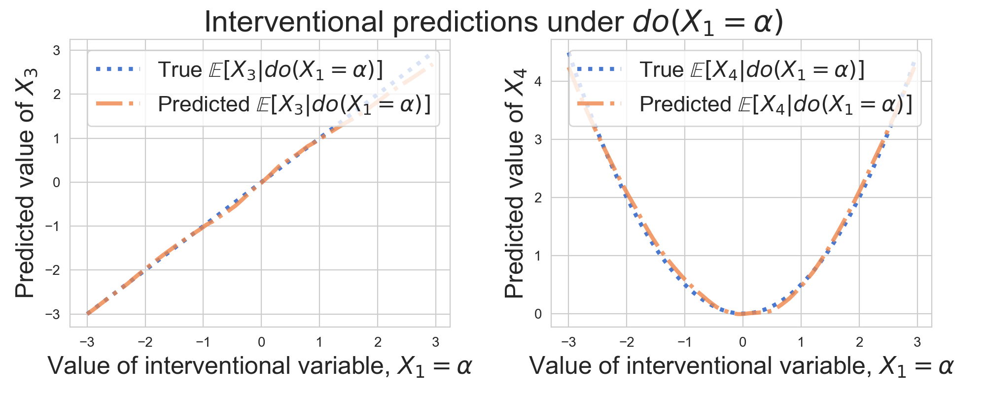
Figure 2: Interventional predictions for variables $X_{3}$ and $X_{4}$ under $do(X_{1}=\alpha)$ for $\alpha\in[-3,3]$. Predicted expectations obtained via an autoregressive flow match the true expectations.

5 Conclusion

We argue that autoregressive flow models are well-suited to causal inference tasks, ranging from causal discovery to making interventional predictions. By interpreting the ordering of variables in an autoregressive flow from a causal perspective we are able to learn causal structure by selecting the ordering with the highest test log-likelihood and present a measure of causal direction based on the likelihood-ratio for nonlinear SEMs. We note that nonlinear SEMs will typically not enjoy the same identifiability guarantees as linear SEMs without further assumptions (Hoyer et al., 2009; Monti and Hyvärinen, 2018; Monti et al., 2019; Khemakhem et al., 2020), and in future work we will explore how such assumptions can be incorporated to flow models. Finally, given a causal ordering, we provide a toy example showing how autoregressive models can be employed to make interventional and counterfactual predictions.

Supplementary

Interventions

Consider an SEM $\mathcal{S}=(\mathbf{S},\mathbb{P}_{\mathbf{n}})$, where $\mathbf{S}$ is a set of $d$ equations like in (1), and $\mathbb{P}_{\mathbf{n}}$ is the distribution of the latent disturbances $\mathbf{n}$. The SEM defines the observational distribution of the random vector $\mathbf{x}$: sampling from $\mathbb{P}_{\mathbf{x}}$ is equivalent to sampling from $\mathbb{P}_{\mathbf{n}}$ and propagating the samples through the system of equations $\mathbf{S}$.

It is possible to manipulate the SEM $\mathcal{S}$ to create interventional distributions over x. This can be done by changing the noise distribution $\mathbb{P}_{\mathbf{n}}$, or by putting a point mass over one (or many) variable $x_{i}$, while keeping the rest of the equations fixed — this latter form was denoted by $\textit{do}(x_{i}=\alpha)$ in the text above.

Interventions are very useful in understanding causal relationships. If intervening on a variable $x_{i}$ changes the marginal distribution of another variable $x_{j}$, then it is very likely that $x_{i}$ has some causal effect on $x_{j}$. Conversely, if intervening on $x_{j}$ doesn’t change the marginal distribution of $x_{i}$, then the latter is not a descendant of $x_{j}$.

In addition, interventions are used to model the distributions we obtain by running randomized experiments. Such experiments are often difficult or unethical to conduct. Interventional SEMs provide a mathematical framework in which such restrictions are alleviated.

Algorithm 1 Generate samples from an interventional distribution

  Input: interventional (root) variable $x_{i}$, intervention value $\alpha$, number of samples $S$

  Infer $n_{i}$ by inverting flow: $n_{i}=f_{i}^{-1}(\alpha)$.

  for $s=1$ to $S$ do

     sample $n_{j}(s)$ from flow base distribution for $j\neq i$

     set $n_{i}(s)=n_{i}$

     generate interventional sample as $x(s)=T(n(s))$, i.e., by passing $z(s)$ through flow.

  end for

  Return: samples $\mathbf{x}=\{x(s):s=1,\ldots,S\}$

Counterfactuals

While structural equation models introduce strong assumptions, they also facilitate the estimation of counterfactual queries. A counterfactual query seeks to quantify statements of the form: what would the value for variable $x_{i}$ have been if variable $x_{j}$ had taken value $\alpha$, given that we have observed $\mathbf{x}=\mathbf{x}^{obs}$? By construction, the value of observed variables $\mathbf{x}$ is fully determined by noise/latent variables $\mathbf{z}$ and the associated structural equations, as described in equation (1). Abusing notation, this may be written as $\mathbf{x}=T(\mathbf{n})$ where $T$ encodes the structural equations. As such, given a set of structural equations and an observation $\mathbf{x}^{obs}$, we follow the notation of Pearl [2009] and write ${x_{i}}_{x_{j}\leftarrow\alpha}(\mathbf{n})$ to denote the value of $x_{i}$ under the counterfactual that $x_{j}\leftarrow\alpha$ given observation $\mathbf{x}^{obs}=T(\mathbf{n}^{obs})$.

The fundamental difference between an interventional and counterfactual query is that the former seeks to marginalize over latent variables, whereas the latter conditions on the latents. The process of obtaining counterfactual predictions is described in Pearl et al. [2009] as consisting of three steps:

1. Abduction: given an observation $\mathbf{x}^{obs}$, infer the conditional distribution/values over latent variables $\mathbf{n}^{obs}$. In the context of an autoregressive flow model this is obtained as $\mathbf{n}^{obs}=T^{-1}(\mathbf{x}^{obs})$.

2. Action: substitute the values of $\mathbf{n}^{obs}$ with the values based on the counterfactual query, $\mathbf{x}_{x_{j}\leftarrow\alpha}$. More concretely, for a counterfactual, $\mathbf{x}_{x_{j}\leftarrow\alpha}$, we replace the structural equations for $x_{j}$ with $x_{j}=\alpha$ and adjust the inferred value of latent $n^{obs}_{j}$ accordingly. As was the case with interventions, if $x_{j}$ is a root node, then we can set $n^{obs}_{j}=f_{j}^{-1}(\alpha)$

3. Prediction: compute the implied distribution over $\mathbf{x}$ by propagating latent variables, $\mathbf{n}^{obs}$, through the structural equation models.

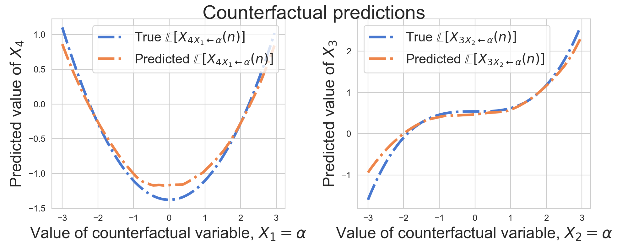
Figure 3: Counterfactual predictions for variables $x_{3}$ and $x_{4}$. Note that flow is able to obtain accurate counterfactual predictions for a range of values of $\alpha\in[-3,3]$.

Toy example

We continue with the simple 4 dimensional structural equation model described in equation (12). We assume we observe $\mathbf{x}^{obs}=(2.00,1.50,0.81,-0.28)$ and consider the counterfactual values under two distinct scenarios:

• the expected counterfactual value $x_{4}$ if instead $x_{1}=\alpha$ for $\alpha\in[-3,3,]$ instead of $x_{1}=2$ as was observed. This is denoted as $\mathbb{E}[{x_{4}}_{x_{1}\leftarrow\alpha}(\mathbf{n})|\mathbf{x}^{obs}]$.

• the expected counterfactual value $x_{3}$ if $x_{2}=\alpha$ for $\alpha\in[-3,3,]$ instead of $X_{2}=1.5$ as was observed. This is denoted as $\mathbb{E}[{x_{3}}_{x_{2}\leftarrow\alpha}(\mathbf{n})|\mathbf{x}^{obs}]$.

As the true structural equations are provided in equation (12), we are able to compute the true counterfactual expectations and compare these to results obtained from an autoregressive flow model. Results, provided in Figure 3, demonstrate the the autoregressive flow model is able to make accurate counterfactual predictions.

Algorithm 2 Generate samples from a counter-factual distribution

  Input: observed data $\textbf{x}^{obs}$, counterfactual (root) variable $x_{i}$ and value $\alpha$

     1. Abduction: Infer $\textbf{n}^{obs}=T^{-1}(\mathbf{x}^{obs})$

     2. Action: Set $n_{j}^{obs}=f_{j}^{-1}(\alpha)$

     3. Prediction: Pass inferred latent variables forward through flow Return: $\mathbf{x}_{x_{j}\leftarrow\alpha}(\mathbf{n}^{obs})=T(\mathbf{n}^{obs})$

References

- Blöbaum et al. [2018] Patrick Blöbaum, Dominik Janzing, Takashi Washio, Shohei Shimizu, and Bernhard Schölkopf. Cause-Effect Inference by Comparing Regression Errors. AISTATS, 2018.
- Dinh et al. [2016] Laurent Dinh, Jascha Sohl-Dickstein, and Samy Bengio. Density estimation using real nvp. arXiv preprint arXiv:1605.08803, 2016.
- Hoyer et al. [2009] Patrik O Hoyer, Dominik Janzing, Joris M. Mooij, Jonas Peters, and Bernhard Schölkopf. Nonlinear causal discovery with additive noise models. Neural Inf. Process. Syst., pages 689–696, 2009.
- Huang et al. [2018] Chin-Wei Huang, David Krueger, Alexandre Lacoste, and Aaron Courville. Neural autoregressive flows. International Conference on Machine Learning, 2018.
- Hyvärinen and Smith [2013] Aapo Hyvärinen and Stephen M Smith. Pairwise Likelihood Ratios for Estimation of Non-Gaussian Structural Equation Models. J. Mach. Learn. Res., 14:111–152, 2013.
- Khemakhem et al. [2020] Ilyes Khemakhem, Diederik Kingma, Ricardo Monti, and Aapo Hyvarinen. Variational autoencoders and nonlinear ICA: A unifying framework. In International Conference on Artificial Intelligence and Statistics, pages 2207–2217, 2020.
- Monti and Hyvärinen [2018] Ricardo Pio Monti and Aapo Hyvärinen. A unified probabilistic model for learning latent factors and their connectivities from high-dimensional data. 34th Conference on Uncertainty in Artificial Intelligence (UAI), 2018.
- Monti et al. [2019] Ricardo Pio Monti, Kun Zhang, and Aapo Hyvärinen. Causal discovery with general non-linear relationships using non-linear ICA. 35th Conference on Uncertainty in Artificial Intelligence (UAI), 2019.
- Mooij et al. [2016] Joris M Mooij, Jonas Peters, Dominik Janzing, Jakob Zscheischler, and Bernhard Schölkopf. Distinguishing cause from effect using observational data: methods and benchmarks. The Journal of Machine Learning Research, 17(1):1103–1204, 2016.
- Neyman and Pearson [1933] Jerzy Neyman and Egon Sharpe Pearson. Ix. on the problem of the most efficient tests of statistical hypotheses. Philosophical Transactions of the Royal Society of London. Series A, 231(694-706):289–337, 1933.
- Papamakarios et al. [2019] George Papamakarios, Eric Nalisnick, Danilo Jimenez Rezende, Shakir Mohamed, and Balaji Lakshminarayanan. Normalizing flows for probabilistic modeling and inference. arXiv preprint arXiv:1912.02762, 2019.
- Pearl [2009] Judea Pearl. Causality. Cambridge University Press, 2009.
- Pearl et al. [2009] Judea Pearl et al. Causal inference in statistics: An overview. Statistics surveys, 3:96–146, 2009.
- Spirtes et al. [2000] Peter Spirtes, Clark Glymour, Richard Scheines, David Heckerman, Christopher Meek, and Thomas Richardson. Causation, Prediction and Search. MIT Press, 2000.
- Zheng et al. [2018] Xun Zheng, Bryon Aragam, Pradeep K Ravikumar, and Eric P Xing. DAGs with NO TEARS: Continuous optimization for structure learning. In Advances in Neural Information Processing Systems, pages 9472–9483, 2018.