DESY 20-120

Dark matter models for the 511 keV galactic line
predict keV electron recoils on Earth

Abstract

We propose models of Dark Matter that account for the 511 keV photon emission from the Galactic Centre, compatibly with experimental constraints and theoretical consistency, and where the relic abundance is achieved via $p$-wave annihilations or, in inelastic models, via co-annihilations. Due to the Dark Matter component that is inevitably upscattered by the Sun, these models generically predict keV electron recoils at detectors on Earth, and could naturally explain the excess recently reported by the XENON1T collaboration. The very small number of free parameters make these ideas testable by detectors like XENONnT and Panda-X, by accelerators like NA64 and LDMX, and by cosmological surveys like the Simons observatory and CMB-S4. As a byproduct of our study, we recast NA64 limits on invisibly decaying dark photons to other particles.

Introduction.

Data that deviate from standard predictions are lifeblood of progress in physics. The past few decades have seen a plethora of such observational ‘anomalies’, both in cosmic rays and in underground detectors, that could have been explained by some property of particle Dark Matter (DM). None of them has been so far enough to claim the discovery of a new DM property, because of the possible alternative explanations in terms of new astrophysical sources, of underestimated systematics, etc, often flavored with a healthy dose of skepticism. An awareness has therefore emerged that the confirmation of a DM origin for some anomaly would require, as a necessary condition, that many anomalies are intimately linked together within a single model of DM.

It is the purpose of this letter to point out one such link. Not only we propose DM models that explain the observed 511 keV line from the Galactic Centre (GC) Prantzos et al. (2011); Siegert et al. (2016); Kierans et al. (2019), but also we show they predict electron recoils with energies of the order of a keV, of the right intensity and spectrum to be observed by XENON1T Aprile et al. (2019, 2020) and to explain the excess seen in Aprile et al. (2020). Our spirit in writing this paper is not to abandon the skepticism praised above, but rather to add an interesting –in our opinion– piece of information to the debates surrounding both datasets.

The 511 keV galactic line.

A 511 keV photon line emission in the galaxy has been observed since the 70’s, recent measurements include that with the SPI spectrometer on the INTEGRAL observatory Siegert et al. (2016) and the one with the COSI balloon telescope Kierans et al. (2019), see Prantzos et al. (2011) for an earlier review. The signal displays two components of comparable intensity, one along the galactic disk and one in the bulge, the latter with an extension of $O(10^{\circ})$ around the galactic center (GC), strongly peaked, corresponding to a flux of $\simeq 10^{-3}$ photons cm^-2 sec^-1 Siegert et al. (2016). The line is attributed to the annihilation of $e^{+}e^{-}$ into $\gamma\gamma$ via positronium formation, thus it requires sources injecting positrons in the regions where the emission is seen, and with injection energy smaller than about 3 MeV Beacom and Yuksel (2006).

The emission from the galactic disk has been tentatively explained with positron injection from the decay of isotopes coming from nucleosynthesis in stars (see e.g. Prantzos et al. (2011); Bartels et al. (2018)), while the origin of the emission in the bulge is still the object of debate (‘one of the most intriguing problems in high energy astrophysics’ Prantzos et al. (2011)). Recent proposals to explain the positron injection include, for example, low-mass X-ray binaries Bartels et al. (2018) and Neutron Star mergers Fuller et al. (2019).

The 511 line and Dark Matter: preliminaries.

Given that the origin of the bulge 511 keV line has not yet been clarified, and given that DM exists in our galaxy, it makes sense to entertain the possibility that the latter is responsible for the former. A DM origin for the positron injection in the bulge has indeed been investigated since Boehm et al. (2004). The morphology of the signal excludes DM decays in favor of annihilations, see e.g. Vincent et al. (2012). The 511 keV line emission in the galactic bulge could be accounted for by self-conjugate DM annihilations into an $e^{+}e^{-}$ pair with

$$\langle\sigma v\rangle_{511}\simeq 5\cdot 10^{-31}\Big{(}\frac{M_{{\rm DM}}}{3~{}\text{MeV}}\Big{)}^{\!2}\,\frac{\text{cm}^{3}}{\text{sec}}\,,$$ (1)

where we have used the best fit provided in Vincent et al. (2012) for an NFW DM density profile, as an indicative benchmark. Different profile shapes and the use of new data for the line could change the precise value of $\langle\sigma v\rangle_{511}$, which however is not crucial for the purpose of this paper.

The need for a positron injection energy smaller than 3 MeV Beacom and Yuksel (2006) implies that, unless one relies on cascade annihilations Jia (2018), $M_{{\rm DM}}\lesssim 3$ MeV. Since so small values of $M_{{\rm DM}}$ have been found to be in conflict with cosmological observations, a simple DM-annihilation origin of the 511 keV line has been claimed excluded in Wilkinson et al. (2016). Recently, however, the refined analysis of Escudero (2019); Sabti et al. (2020) found that values of $M_{{\rm DM}}$ down to $\sim 1$ MeV can be made consistent with CMB and BBN, by means of a small extra neutrino injection in the early universe, simultaneous with the electron one from the DM annihilations. We will rely on this new result in building DM models for the 511 keV line.

Eq. (1) clarifies that $s$-wave DM annihilation cannot explain the 511 keV line, because so small cross sections imply overclosure of the universe. To be compatible with a thermal generation of the DM abundance, one therefore needs annihilation cross sections in the early universe much larger than today in the GC. This is realised for example in two simple pictures, where the DM relic abundance is set by:

• $p$-wave annihilations;

• coannihilations with a slightly heavier partner.

We will build explicit DM models that realise each of them in the next two paragraphs.

DM for the 511 keV line: $p$-wave.

Using $\langle\sigma v\rangle_{\text{relic}}^{(p)}(M_{{\rm DM}}=2~{}\text{MeV})\simeq 2.2\cdot 10^{-25}v_{\text{rel}}^{2}\text{cm}^{3}/\text{sec}$ Saikawa and Shirai (2020), we find

$$M_{{\rm DM}}^{(p)}\simeq 2~{}\text{MeV}\frac{\langle v_{\text{rel}}^{2}\rangle^{1/2}_{\text{bulge}}}{1.1\times 10^{-3}}\,,$$ (2)

where we have normalised $\langle v_{\text{rel}}^{2}\rangle^{1/2}_{\text{bulge}}$ to the value obtained from the velocity dispersion in the bulge $\sigma\simeq 140$ km/s Valenti et al. (2018) , and where we have assumed that the dominant annihilation channel at freeze-out is $e^{+}e^{-}$. Note that the preferred DM mass would be the same for non-self-conjugate annihilating DM, for which both $\langle\sigma v\rangle_{511}$ and $\langle\sigma v\rangle_{\text{relic}}$ are larger by a factor of 2.

An explicit model realising this picture consists of a Majorana fermion $\chi$ as DM candidate, whose interactions with electrons are mediated by a real scalar $S$ via the low-energy Lagrangian (we use 2 component spinor notation throughout this work)

$$\mathcal{L}=y_{\rm D}\chi^{2}S+g_{e}e_{\rm L}e^{\dagger}_{\rm R}S+\text{h.c.}\,.$$ (3)

This results in the annihilation cross section

$$\sigma v_{e^{+}e^{-}}=v_{\text{rel}}^{2}\frac{(y_{\rm D}g_{e})^{2}}{8\pi}\frac{M_{{\rm DM}}^{2}\,\big{(}1-m_{e}^{2}/M_{{\rm DM}}^{2}\big{)}^{\!\frac{3}{2}}}{\big{(}m^{2}_{\rm S}-4M_{{\rm DM}}^{2}\big{)}^{2}+m^{2}_{\rm S}\,\Gamma^{2}_{\rm S}}\,,$$ (4)

and in the cross section for DM-$e$ elastic scattering

$$\sigma_{e}=\frac{(y_{\rm D}g_{e})^{2}}{\pi}\frac{\mu_{e{\rm DM}}^{2}}{m^{4}_{\rm S}}\,,$$ (5)

where $m_{\rm S}$ is the scalar mass, $\Gamma_{\rm S}$ its width, and $\mu_{e{\rm DM}}=m_{e}M_{{\rm DM}}/(m_{e}+M_{{\rm DM}})$. Once $\sigma v_{e^{+}e^{-}}$ and $M_{{\rm DM}}$ are fixed by the requirements to fit the 511 keV line eq. (1) and to reproduce the correct relic abundance eq. (2), then only two free parameters are left, which we choose as $g_{e}$ and $m_{\rm S}$ in Fig. 1. We find that a region capable of explaining the 511 keV line exists, delimited by perturbativity, direct detection (derived later) and collider limits (see the Appendix A).

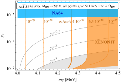
Figure 1: Once the conditions to reproduce the DM abundance and the 511 keV line are imposed, the phenomenology of the model is entirely determined by the scalar mediator mass $m_{\rm S}$ and its coupling to electrons $g_{e}$. Shaded: non-perturbative dark coupling (gray), our recast of NA64 dark photon limit Banerjee et al. (2019) (blue), indicative limit from XENON1T data Aprile et al. (2019) (orange). Lines: contours of constant $\sigma_{e}$ (orange) and of constant dark coupling $y_{\rm D}$ (gray). The thick orange line corresponds to $\sigma_{e}=4\cdot 10^{-38}$ cm², which induces the electron recoil spectrum at XENON1T shown in Fig. 3.

The existence of 3 degrees of freedom with masses $M_{{\rm DM}}$ and $m_{\rm S}$ of a few MeV is not in conflict with cosmological data, provided one posits a small injection of neutrinos in the early universe in a proportion $\sim 1:10^{4}$ to the electron injection, see Escudero (2019); Sabti et al. (2020). This can for example be achieved with a coupling to neutrinos, $g_{\nu}\nu^{2}S$, of size $g_{\nu}\sim 10^{-2}g_{e}$, and where $g_{e}\sim 10^{-6}$ in the region allowed by the various limits, see Fig. 1. Coupling of neutrinos and electrons of these sizes can be easily obtained in electroweak-invariant completions of the Lagrangian of eq. (3). Since they do not present any particular model-building challenge, we defer their presentation to Appendix B. The results of Escudero (2019); Sabti et al. (2020) indicate that agreement with cosmological data fixes that ratio up to roughly one order of magnitude, so in this sense we do not need a very precise tuning between the electron and neutrino couplings.

Coming to future tests of this model, direct detection experiments like XENONnT and Panda-X will play a leading role in testing the available parameter space of Fig.1. We stress that the shape of the electron recoil spectrum is fixed over the entire parameter space, only its normalisation changes according to the DD cross section shown by the orange lines. LDMX Åkesson et al. (2018) will further cut in the available parameter space, as it can probe invisibly decaying dark photon with $m_{V}=15~{}{\rm MeV}$ down to $\epsilon=10^{-6}$, corresponding to $g_{e}$ of the same order (see Appendix B). Finally, according to Ref. Sabti et al. (2020), both CMB-S4 Abazajian et al. (2019) and the Simons Observatory Ade et al. (2019) will probe $M_{{\rm DM}}=2$ MeV at 95%CL or more and regardless of the ratio of the electron and neutrino couplings, thus offering useful complementary information.

DM for the 511 keV line: coannihilations.

As a model that concretely realises this idea, we add to the SM a gauge group $U(1)^{\prime}$, two fermions $\xi$ and $\eta$ with charges 1 and -1 respectively, and a scalar $\phi$ with charge 2 that spontaneously breaks the symmetry. The most general low-energy Lagrangian that preserves charge conjugation ($\eta\leftrightarrow\xi$, $\phi\leftrightarrow\phi^{*}$, $V_{\mu}\leftrightarrow-V_{\mu}$) reads

$$\mathcal{L} = V(|\phi|)+\frac{\epsilon}{2}V_{\mu\nu}F^{\mu\nu}+(ig_{\rm D}\chi_{2}^{\dagger}\bar{\sigma}_{\mu}\chi_{1}V^{\mu}+\text{h.c.})$$ (6)

$$- \frac{\bar{m}}{2}(\chi_{1}^{2}+\chi_{2}^{2})-\frac{y_{\phi}}{2}(\phi+\phi^{*})\big{(}\chi_{2}^{2}-\chi_{1}^{2}\big{)}+\text{h.c.}\,,$$

where $\chi_{1}=i(\eta-\xi)/\sqrt{2}$ and $\chi_{2}=(\eta+\xi)/\sqrt{2}$ are the Majorana mass eigenstates, $F_{\mu\nu}$ is the electromagnetic field strength and we have understood all kinetic terms. The scalar mass and triple-coupling read

$$V(|\phi|)=\lambda_{\phi}\Big{(}|\phi|^{2}-\frac{v_{\phi}^{2}}{2}\Big{)}^{\!2}\;\Rightarrow\;m_{\varphi}^{2}=2\lambda_{\phi}v_{\phi}^{2}\,,\;\lambda_{\varphi^{3}}=6\lambda_{\phi}v_{\phi}\,,$$ (7)

where $\phi=(\varphi+v_{\phi})/\sqrt{2}$ and $\lambda_{\varphi^{3}}$ is defined by $\mathcal{L}\supset\lambda_{\varphi^{3}}\varphi^{3}/6$. The physical vector and fermion masses read

$$m_{V}=2g_{\rm D}v_{\phi},\qquad m_{1,2}=\bar{m}\pm\frac{\delta}{2},\qquad\delta=2\,\sqrt{2}\,y_{\phi}v_{\phi}.$$ (8)

$\chi_{1}$ coannihilates with $\chi_{2}$ via dark photon exchange. In the limit $\delta\ll m_{1,2}=M_{{\rm DM}}$, one finds

$$\sigma v_{\chi_{1}\chi_{2}\to e^{+}e^{-}}=4\alpha_{e}\epsilon^{2}g^{2}_{\rm D}\frac{M_{{\rm DM}}^{2}+m_{e}^{2}/2}{(m_{V}^{2}-4M_{{\rm DM}}^{2})^{2}}\sqrt{1-\frac{m_{e}^{2}}{M_{{\rm DM}}^{2}}}\,,$$ (9)

where $\alpha_{e}$ is the fine-structure constant. For definiteness, we then assume that $\chi_{2}$ decays on cosmological scales, such that coannihilations cannot be responsible for a positron injection in the GC today. We will come back to this point in the end of the paragraph.

One can then explain the 511 keV line, if $m_{\varphi}<M_{{\rm DM}}$ and $\varphi$ decays to $e\bar{e}$, via pair annihilations $\chi_{i}\chi_{i}\to\varphi\varphi$. The associated cross section, at first order in $y_{\phi}v_{\phi}/\lambda_{\varphi^{3}}\ll 1$, reads ($i=1,2$)

$$\sigma v_{\chi_{i}\chi_{i}\to\varphi\varphi}=v_{\text{rel}}^{2}\frac{y_{\phi}^{2}\,\lambda_{\varphi^{3}}^{2}}{64\pi}\frac{1}{(4\,m_{i}^{2}-m_{\varphi}^{2})^{2}}\sqrt{1-\frac{m_{\phi}^{2}}{m_{i}^{2}}}\,.$$ (10)

An operator $|\phi|^{2}(e_{\rm L}e^{\dagger}_{\rm R}+\text{h.c.})/\Lambda_{\phi e}$ with $\Lambda_{\phi e}\sim 10^{9-10}v_{\phi}$ guarantees that $\varphi$ decays to $e\bar{e}$ instantaneously on astrophysical scales, while being allowed by collider, supernovae and BBN limits Krnjaic (2016); Dev et al. (2020). It could originate –at the price of some tuning– from a $|\phi|^{2}|H|^{2}$ term, or from the models discussed in Appendix B. Since a $\chi_{1}\chi_{1}$ annihilation injects two $e\bar{e}$ pairs, the cross section that best fits the 511 keV line is reduced by a factor of 2 with respect to eq. (1). Therefore we impose

$$\sigma v_{\chi_{i}\chi_{i}\to\varphi\varphi}=\frac{1}{2}\langle\sigma v\rangle_{511}\,\frac{v_{\text{rel}}^{2}}{\langle v_{\text{rel}}^{2}\rangle_{\text{bulge}}}\,.$$ (11)

If $\chi_{i}\chi_{i}\to\varphi\varphi$ were the only processes responsible for the DM abundance, then we would have found another realisation of the $p$-wave annihilating idea, just with $M_{{\rm DM}}\simeq 4$ MeV. It follows that, for $M_{{\rm DM}}\lesssim 4$ MeV, the DM relic density is set dominantly by coannihilations. We then fix $\epsilon$ by the simple requirement

$$\sigma v_{e^{+}e^{-}}+3\frac{\sigma v_{\chi_{i}\chi_{i}\to\varphi\varphi}/v_{\text{rel}}^{2}}{x_{\rm FO}}=\sigma v^{(s)}_{\rm FO}\,,$$ (12)

where the left-hand side sums the $s$- and $p$-wave contributions (see e.g. Kolb and Turner (1990) for the origin of the relative factors) and where we use for simplicity the $s$-wave values at $M_{{\rm DM}}=3$ MeV, $\sigma v^{(s)}_{\rm FO}\simeq 8\times 10^{-26}\text{cm}^{3}/\text{sec}$ Saikawa and Shirai (2020) and $x_{\rm FO}\simeq 15$ (their dependence on $M_{{\rm DM}}$ is very mild).

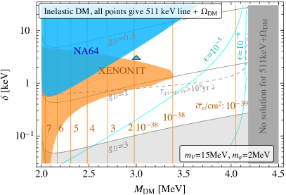
Figure 2: The conditions to reproduce the DM abundance and the 511 keV line impose $M_{{\rm DM}}\lesssim 4$ MeV and leave 4 free parameters, chosen here as $M_{{\rm DM}}$, $\delta$, $m_{\varphi}$ and $m_{V}$. Shaded: non-perturbative dark coupling (gray), NA64 limit Banerjee et al. (2019) (blue), indicative limit from XENON1T data Aprile et al. (2020) (orange). Lines: $\bar{\sigma}_{e}$ (orange), $g_{\rm D}$ (gray), $\epsilon$ (cyan). The dashed gray line roughly delimits the region where $\chi_{2}$ decays into neutrinos are not enough to deplete the primordial $\chi_{2}$ population, and further constraints could arise. The blue triangle corresponds to the electron recoil spectrum at XENON1T shown in Fig. 3, and it explains the excess events presented in Aprile et al. (2020).

The model is then left with 4 free parameters, we visualise its parameter space in Fig. 2 for the benchmark values $m_{\varphi}=2$ MeV and $m_{V}=15$ MeV. The allowed region is again delimited by perturbativity, direct detection and collider limits. Analogously to the previous model, these low values of $M_{{\rm DM}}$ can be brought in agreement with BBN and CMB data by a coupling $g_{\nu}V_{\mu}\nu^{\dagger}\bar{\sigma}^{\mu}\nu$, with $g_{\nu}\sim 10^{-2}e\epsilon$. We refer the reader to the Appendix B for a possible origin of $g_{\nu}$. Here we just point out that it induces $\Gamma_{\chi_{2}\to\chi_{1}\bar{\nu}\nu}\simeq g^{2}_{\nu}g^{2}_{\rm D}\delta^{5}/(40\pi^{3}m_{V}^{4})$, which for $m_{V}=15$ MeV and $\delta\gtrsim 1$ keV implies $\tau_{2}<10^{9}$ years, so that all $\chi_{2}$’s left after freeze-out have decayed by today. Larger values of $\tau_{2}$ can be avoided by adding another operator to mediate $\chi_{2}$ decays (e.g. a dipole), otherwise values of $\delta\lesssim 1$ keV could potentially be in conflict with searches for the primordial population of $\chi_{2}$ Baryakhtar et al. (2020).

The allowed values of $\delta$ are restricted around a few keV, which is particularly interesting because they could explain Baryakhtar et al. (2020) the excess events at XENON1T Aprile et al. (2020), as we explicitly derive in the next paragraph. The event rate at XENON1T is proportional to the cross section $\chi_{2}e\to\chi_{1}e$ in the limit $\delta\to 0$,

$$\bar{\sigma}_{e}=4\alpha_{e}g^{2}_{\rm D}\epsilon^{2}\frac{\mu_{e{\rm DM}}^{2}}{m_{V}^{4}}\,,$$ (13)

which we also display in Fig. 2.

Fig. 2 also reports the aforementioned collider limits, and clarifies the impact that future experiments could have in testing this model. The LDMX sensitivity to dark photons will allow to almost completely probe the available parameter space. Cosmological surveys and especially DD experiments will be sensitive to a sizeable chunk of the parameter space, and thus will play an important complementary role in confirming or refuting our interpretation of the 511 keV GC line.

Finally, we left out of this study the case where there is a residual population of $\chi_{2}$ today, which has also been shown to possibly explain the excess events at XENON1T Harigaya et al. (2020); Lee (2020); Bramante and Song (2020); Baryakhtar et al. (2020); Bloch et al. (2020); An and Yang (2020); Baek et al. (2020); He et al. (2020). While this goes beyond the purpose of this work, it would be interesting to investigate it in combination with the 511 keV line and we plan to come back to it in future work.

keV electron recoils from Sun-upscattered DM.

The models we proposed to explain the 511 keV line require DM with a mass of a few MeV, interacting with electrons. Such a DM is efficiently heated inside the sun, resulting in a flux of solar-reflected DM with kinetic energy ($\sim\mathrm{keV}$) significantly larger than the one of halo DM, thus offering new detection avenues to direct detection experiments An et al. (2018). We now show that, via this higher-energy component, both ‘$p$-wave’ and ‘coannihilations’ models for the 511 keV line automatically induce electron-recoil signals that are probed by XENON1T S2-only Aprile et al. (2019) and S1$+$S2 Aprile et al. (2020) data.

We outline the procedure to obtain the event rate caused by the solar-reflected DM flux and refer to the Appendix C for more details. In the case of our interest with relatively small $\sigma_{e}$, the solar-reflected DM flux $\Phi_{\mathrm{refl}}$ is estimated as

$$\frac{d\Phi_{\mathrm{refl}}}{dE}\simeq\frac{n_{\rm DM}}{\left(1\mathrm{AU}\right)^{2}}\int_{0}^{r_{\mathrm{sun}}}\!\!dr\,r^{2}\frac{v_{\mathrm{esc}}(r)}{v_{\rm DM}}\,n_{e}(r)\left\langle\frac{d\sigma_{e}}{dE}v_{e}(r)\right\rangle,$$ (14)

where $E$ is the DM kinetic energy, $n_{\rm DM}$ is the DM number density, $r_{\mathrm{sun}}$ is the solar radius, $v_{\mathrm{esc}}$ is the escape velocity, $v_{\rm DM}$ is the halo DM velocity, $n_{e}$($v_{e}$) is the electron number density (velocity), and $\langle...\rangle$ denotes the thermal average. In this formula, we have improved the analysis of Baryakhtar et al. (2020) by including the radial dependence of the solar parameters, taken from Bahcall et al. (2005). The recoil spectrum of the electron initially in the $(n,l)$ state of a XENON atom is given by

$$\frac{dR_{nl}}{dE_{R}} =\frac{N_{T}{\sigma}_{e}}{8\mu_{e{\rm DM}}^{2}E_{R}}\int dq\,q\left\lvert f_{nl}\right\rvert^{2}\xi\left(E_{\mathrm{min}}\right),$$ (15)

$$\xi\left(E_{\mathrm{min}}\right) =\int_{E_{\mathrm{min}}}\!\!dE\,\left(\frac{M_{{\rm DM}}}{2E}\right)\frac{d\Phi_{\mathrm{refl}}}{dE},$$ (16)

$$E_{\mathrm{min}} =\frac{M_{{\rm DM}}}{2}\left(\frac{E_{nl}+E_{R}-\delta}{q}+\frac{q}{2M_{{\rm DM}}}\right)^{2},$$ (17)

where $N_{T}$ is the number of target particles and $E_{nl}$ is the electron binding energy, see e.g. Essig et al. (2016) for a detailed derivation of the above expressions. We compute the atomic form factor $f_{nl}$ following Essig et al. (2012); Bloch et al. (2020), and leave a refined treatment including relativistic effects Roberts et al. (2016); Roberts and Flambaum (2019) to future work.

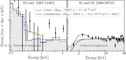
Figure 3: Electron recoil spectra induced by solar-upscattered DM, for two benchmark values of the parameters of models that explain the 511 keV line. We overlay them with data and expected backgrounds from the XENON1T S2 Aprile et al. (2019) (left) and S1+S2 Aprile et al. (2020) (right) analyses.

In Fig. 3, we show the electron recoil spectra for two benchmark points $M_{{\rm DM}}=2\,\mathrm{MeV}$ and $\sigma_{e}=4\times 10^{-38}\,\mathrm{cm}^{2}$ in the $p$-wave case and $M_{{\rm DM}}=3\,\mathrm{MeV}$, $\sigma_{e}=1.9\times 10^{-38}\,\mathrm{cm}^{2}$ and $\delta=3\,\mathrm{keV}$ in the coannihilation case. The induced electron recoils peak at energies below 2 keV in the $p$-wave case, and in the coannihilation one if $\delta\lesssim$ keV. In the former case, the position of the peak is fixed by the dark matter mass Eq. (2), and it does not appear possible to explain signal excess observed at XENON1T. On the other hand, in the latter case with larger $\delta$ the events instead peak at $E_{R}\sim\delta$, because the downscattering $\chi_{2}\rightarrow\chi_{1}$ releases more energy than the initial one of $\chi_{2}$. In particular, the events are peaked at $E_{R}=2$–$3\,\mathrm{keV}$ in our benchmark point, which can explain the recent XENON1T anomaly. We emphasize that this result is non-trivial, because the allowed parameter region is defined by requirements and experimental limits that are completely independent of XENON1T. It is then a fortunate accident that this region is in the right ballpark for the explanation of the XENON1T anomaly.

The results of this paragraph are of course interesting beyond these anomalies, as they quantify how XENON1T tests models of light electrophilic DM. The limits shown in Figs. 1 and 2 are derived by the conservative requirement that signal plus background should not overshoot the data in Aprile et al. (2020) by more than 3$\sigma$, a more precise limit derivation is left to future work.

Conclusions and Outlook.

We have presented two models which explain the 511 keV line in the galactic bulge by annihilation of particle dark matter with a mass of order MeV. The relic abundance is set by p-wave annihilations in one model, and by coannihilations with a slightly heavier partner in the other model. We have found the novel result that these models induce electron recoils on Earth that are being tested by XENON1T, and that coannihilationmodels could, non-trivially, simultaneously explain the 511 keV line and the excess events recently presented by XENON1T Aprile et al. (2020). In addition, we have demonstrated that both models are compatible with all experimental constraints, in particular with cosmological ones: to evade the conclusion of Wilkinson et al. (2016) that no ${\cal O}({\rm MeV})$ DM model could explain the 511 keV line, we have relied on an extra annihilation channel into neutrinos and on the new results of Escudero (2019); Sabti et al. (2020).

Independently of the XENON1T anomaly, our proposed DM explanations of the 511 keV constitute a new physics case for experiments sensitive to keV electron recoils, like XENONnT and Panda-X Fu et al. (2017), for accelerators like NA64 and LDMX Åkesson et al. (2018), and for cosmological surveys like CMB-S4 Abazajian et al. (2019) and the Simons Observatory Ade et al. (2019). The origin of a long-standing astrophysical mystery could be awaiting discovery in their data.

Appendix A Recast of NA64 limits.

NA64 sets the strongest existing constraints on invisibly decaying dark photons in Banerjee et al. (2019): the kinetic mixing $\epsilon$, defined as in eq. (6), should be smaller than an $m_{V}$-dependent function that we denote $\epsilon_{\text{limit}}(m_{V})$. As we are not aware of any recast of those limits to other invisibly decaying light particles, we perform that recast ourselves, for completeness for scalars $S$, pseudoscalars $A$ and axial vectors $V_{A}$, with couplings

$$\mathcal{L}_{\rm S} = g_{e}S\,e^{\dagger}_{\rm L}e_{\rm R}+\text{h.c.},$$ (18)

$$\mathcal{L}_{\rm A} = ig_{e}A\,e^{\dagger}_{\rm L}e_{\rm R}+\text{h.c.},$$ (19)

$$\mathcal{L}_{V_{\rm A}} = ig_{e}V^{\mu}_{\rm A}\,(e^{\dagger}_{\rm R}\bar{\sigma}_{\mu}e_{\rm R}-e^{\dagger}_{\rm L}\bar{\sigma}_{\mu}e_{\rm L}),$$ (20)

which in 4-component spinor notation read, respectively, $g_{e}\bar{e}eS$, $ig_{e}\bar{e}eA$ and $ig_{e}\bar{e}\gamma_{\mu}\gamma_{5}eV^{\mu}_{\rm A}$. We recast NA64 limits by imposing

$$g_{e}(m_{{\rm S},{\rm A},{V_{\rm A}}})<C_{{\rm S},{\rm A},{V_{\rm A}}}e\,\epsilon_{\text{limit}}(m_{{\rm S},{\rm A}}),$$ (21)

where $e$ is the electric charge and

$$C_{X}=\left(\frac{N_{V}/(\epsilon^{2}e^{2})}{N_{X}/g_{e}^{2}}\right)^{\!\frac{1}{2}}\,.$$ (22)

We have defined

$$N_{X}=\int_{0.5}^{x_{\text{max}}}\!\!dx\,\text{Eff}(x)\,\frac{d\sigma}{dx}(eZ\to eZX)\,,$$ (23)

where $x=E_{X}/E_{\text{beam}}$ ($E_{\text{beam}}=100$ GeV for NA64) and the lower limit of integration in $x$ comes from the cut $E_{\text{miss}}>50$ GeV Banerjee et al. (2019). The upper limit of integration $x_{\text{max}}$ satisfies $x_{\text{max}}<0.997$, because of the trigger $E_{\text{cal}}>0.3$ GeV Banerjee et al. (2018). For the cross sections $d\sigma(eZ\to eZX)/dx$ we use the “improved Weizsaecker-Williams” approximations given in eq. (33) of Liu et al. (2017) for $X=S$ and in eq. (30) of Liu and Miller (2017) for $X=V,A,V_{\rm A}$. In Fig. 4 we display the ratio of the $X=S,A,V_{\rm A}$ cross sections and the $X=V$ cross section, the latter being the relevant one for the model on which NA64 has cast its limit.

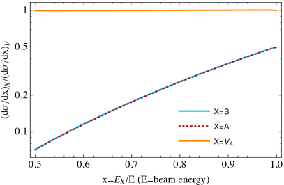
Figure 4: Ratios of cross sections $d\sigma(eZ\to eZX)/dx$, with $x=E_{X}/E_{\text{beam}}$ ($E_{\text{beam}}=100$ GeV for NA64). Numerator: $X=S$ (blue), $A$ (dotted-red), $V_{A}$ (orange); denominator: $X=V$. The range $x\geq 0.5$ is the one relevant for the NA64 searches Banerjee et al. (2019) that we are recasting here. We use the cross sections in the “improved Weizsaecker-Williams” approximations as given in Liu et al. (2017); Liu and Miller (2017). All curves assume $m_{X}=10$ MeV, the dependence on $m_{X}$ is within the thickness of each line for $m_{X}>8$ MeV, and within $\sim 20\%$ of each line for $m_{X}>3$ MeV.

Finally, the efficiency $\text{Eff}(x)$ has a weak dependence on $x$ Banerjee et al. (2019), it does so mostly for $x$ close to one, see the discussion in Banerjee et al. (2018) and e.g. Fig. 11 in that paper. Since we have not found a detailed study of the efficiency of NA64 in the region $x$ close to 1, we assume it is independent of $x$, so that it simplifies in the ratio $N_{V}/N_{X}$ that defines our rescaling eq. (22). As visible in Fig. 4, this procedure does not introduce any significant error for the axial vector case. For the scalar and pseudoscalar cases, since the ratios of their cross sections to the vector one are a monotonically increasing function of $x$, and since the efficiency worsens when $x$ approaches one, the value of $C_{{\rm S},{\rm A}}$ that we obtain for $x_{\text{max}}=0.997$ represent an aggressive estimate of the NA64 exclusion of such particles. A conservative one can instead be obtained by choosing a value of $x_{\text{max}}$ below which the efficiency is roughly a constant in $x$, which we take for definiteness as $x_{\text{max}}=0.9$. Our resulting coefficients $C_{{\rm S},{\rm A},{V_{\rm A}}}$, for these two extreme limits of integration and for various values of $m_{X}$, are given in Table 1. In the $p$-wave model studied in the main text, in order to be conservative on the allowed parameter space, we have used the aggressive rescaling of the NA64 limits, i.e. $C_{\rm S}=1.6$.

$m_{X}$ [MeV]	$C_{\rm S}$		$C_{\rm A}$		$C_{V_{\rm A}}$
	0.997	0.9	0.997	0.9	0.997	0.9	$x_{\text{max}}$
1	1.7	1.8	1.8	2.0	0.8	0.8
2	1.7	2.0	1.7	2.0	0.9	0.9
3	1.6	2.0	1.7	2.1	1.0	1.0
4	1.6	2.0	1.7	2.1	1.0	1.0
5	1.6	2.0	1.6	2.1	1.0	1.0
$\geq 6$	1.6	2.1	1.6	2.1	1.0	1.0

Table 1: Coefficients entering eq. (21) to recast NA64 limits, on invisibly decaying dark photons Banerjee et al. (2019), to invisibly decaying scalars S, pseudoscalars A and axial vectors $V_{\rm A}$ coupled with electrons as in eq. (21). We display our results for two cases of the upper limit of integration $x_{\text{max}}$ in eq. (23).

Another source of uncertainty of our rescaling comes from the fact we used cross sections in the “improved Weizsaecker-Williams” approximation. The comparisons of these cross sections with the full results, in ref. Liu et al. (2017); Liu and Miller (2017), show that the impact of the approximation over the full $x$ range is analogous for the four cases $X=S,A,V,V_{\rm A}$, as one could roughly expect by observing that this approximation consists in a different treatment of the phase-space edges. Therefore the error in our rescaling, induced by the approximations in the cross section, is qualitatively expected to be smaller than the error in the cross sections themselves, because it relies on ratios. Since this recast is not the main purpose of this paper, we content ourselves with this procedure, and we encourage the NA64 collaboration to present their very interesting results for particles other than dark photons.

Appendix B UV completions.

We here propose explicit ultraviolet (UV) completions of all the low-energy couplings that are not manifestly electroweak (EW) invariant.

We start by scalar couplings to electrons. A coupling $g_{e}$ defined as in eq. (3), $g_{e}e_{\rm L}e^{\dagger}_{\rm R}S+\text{h.c.}$, of the needed size $g_{e}\sim 10^{-6}$ (see Fig. 1), can be obtained by adding to the SM two fermions $E_{\rm L}$ and $E^{\dagger}_{\rm R}$, with charge assignments of $e_{\rm R}$ and $e^{\dagger}_{\rm R}$ respectively, and Lagrangian

$$\mathcal{L}_{\rm E}=y_{\rm E}\ell H^{\dagger}E^{\dagger}_{\rm R}+M_{\rm E}E_{\rm L}E^{\dagger}_{\rm R}+g_{\rm E}SE_{\rm L}e^{\dagger}_{\rm R}\,.$$ (24)

This induces a coupling to electrons ($v_{\rm EW}\simeq 246$ GeV)

$$g_{e}\simeq g_{\rm E}\frac{y_{\rm E}v_{\rm EW}}{\sqrt{2}M_{\rm E}}\approx 2\cdot 10^{-6}y_{\rm E}g_{\rm E}\frac{10^{5}~{}\text{TeV}}{M_{\rm E}}\,,$$ (25)

which is of the desired size for $M_{\rm E}$ out of experimental reach and perturbative values of the couplings $y_{\rm E}$ and $g_{\rm E}$.

In the coannihilation model the higher dimensional operator $|\phi|^{2}(e_{\rm L}e^{\dagger}_{\rm R}+\text{h.c.})/\Lambda_{\phi e}$, that induces the coupling of $\varphi$ to electrons, can be obtained by adding to the SM the fermions $E_{\rm L}$ and $E^{\dagger}_{\rm R}$, with SM charge assignments of $e_{\rm R}$ and $e^{\dagger}_{\rm R}$ respectively, and $L_{\rm L}$ and $L^{\dagger}_{\rm R}$, with SM charge assignments of $\ell$ and $\ell^{\dagger}$ respectively. Furthermore, we assign to $E_{\rm L}$ and $L_{\rm L}$ ($E^{\dagger}_{\rm R}$ and $L^{\dagger}_{\rm R}$) charge $+2$ ($-2$) under the $U(1)^{\prime}$ gauge group. The Lagrangian

$$\mathcal{L} = M_{\rm L}L_{\rm L}L^{\dagger}_{\rm R}+M_{\rm E}E_{\rm L}E^{\dagger}_{\rm R}+y_{\rm L}L_{\rm L}H^{\dagger}E^{\dagger}_{\rm R}$$ (26)

$$+ g_{\rm E}\phi E_{\rm L}e^{\dagger}_{\rm R}+g_{\rm L}\phi L_{\rm L}\ell^{\dagger}+\text{h.c.}\,,$$

then induces

$$\frac{\Lambda_{\phi e}}{v_{\phi}}\simeq\frac{M_{\rm L}M_{\rm E}}{y_{\rm L}g_{\rm E}g_{\rm L}v_{\rm EW}v_{\phi}}\approx 10^{9}\frac{g_{\rm D}}{y_{\rm L}g_{\rm E}g_{\rm L}}\frac{15~{}\text{MeV}}{m_{V}}\frac{M_{\rm L}M_{\rm E}}{(40~{}\text{TeV})^{2}}\,,$$ (27)

where we remind the reader that we needed $\Lambda_{\phi e}/v_{\phi}$ in the ballpark of $10^{9-10}$, in order for $\varphi$ to decay to $e\bar{e}$ instantaneously on astrophysical scales and compatibly with collider, supernovae and BBN limits Krnjaic (2016); Dev et al. (2020). We have just seen how this value can be achieved by adding new vector-like leptons with masses out of collider reach.

Otherwise the coupling to electrons of both $S$ and $\varphi$ can easily be obtained via operators that mix the new scalars with the Higgs, respectively $S|H|^{2}$ and $|\phi|^{2}|H|^{2}$. In the latter case, however, one would need to tune the parameters of $V(|\phi|)$ with this quartic coupling, in order to keep $v_{\phi}\ll v_{\rm EW}$.

A coupling of $S$ to neutrinos $g_{\nu}\nu^{2}S$, of size $g_{\nu}\sim 10^{-2}g_{e}$ as needed to make the model compatible with cosmological data Escudero (2019); Sabti et al. (2020), can be achieved by extending the SM with three singlet fermions $\nu_{\rm R}$, $N_{\rm L}$ and $N_{\rm R}$. The EW-invariant Lagrangian

$$\mathcal{L}=y_{\nu}\ell H\nu^{\dagger}_{\rm R}+m_{\rm N}N_{\rm L}N^{\dagger}_{\rm R}+g_{\rm N}SN_{\rm L}\nu^{\dagger}_{\rm R}+\text{h.c.}\,$$ (28)

then induces

$$g_{\nu}\simeq g_{\rm N}\frac{y_{\nu}v_{\rm EW}}{\sqrt{2}M_{\rm N}}\approx 2\cdot 10^{-8}y_{\nu}g_{\rm N}\frac{10^{7}~{}\text{TeV}}{M_{\rm N}}\,,$$ (29)

which is of the desired size $g_{\nu}\sim 10^{-2}g_{e}\sim 10^{-8}$ (see Fig. 1 for the interesting values of $g_{e}$) for $N$ out of experimental reach.

We finally provide an example of an EW-invariant completion for the small coupling to neutrinos of a $U(1)^{\prime}$ gauge boson. We add to the model of eq. (6) one total singlet fermion $\nu^{\dagger}_{\rm R}$ and two left-handed fermions $N_{\rm L}$ and $N_{\rm R}$, with charges respectively $+2$ and $-2$ under $U(1)^{\prime}$, and singlets under the SM gauge group. The Lagrangian

$$\mathcal{L}_{\nu}=y_{\nu}\ell H^{\dagger}\nu^{\dagger}_{\rm R}+m_{\rm N}N^{\dagger}_{\rm L}N_{\rm R}+y_{\rm N}N_{\rm L}\nu_{R}^{\dagger}\phi+\text{h.c.}\,$$ (30)

then induces a coupling of size

$$g_{\nu}\simeq 2\,g_{\rm D}\Big{(}\frac{y_{\rm N}v_{\phi}}{m_{\rm N}}\Big{)}^{2}\approx 10^{-7}\frac{y^{2}_{\rm N}}{g_{\rm D}}\Big{(}\frac{m_{V}}{15~{}\text{MeV}}\Big{)}^{\!2}\Big{(}\frac{30~{}\text{GeV}}{m_{\rm N}}\Big{)}^{\!2}\,.$$ (31)

One can then obtain the needed value $g_{\nu}\sim 10^{-2}e\epsilon\sim 10^{-7}$ (see Fig. 2 for the interesting values of $\epsilon$) for $m_{\rm N}\sim 30$ GeV, which is out of experimental reach because $N$ is a total SM singlet.

Appendix C Solar-reflected DM events at XENON1T.

Here we give the procedure to compute the electron recoil spectra at XENON1T in detail.

The solar-reflected DM flux is given by eq. (14), and we explain each term in the following. We take the DM number density as $n_{\mathrm{DM}}=(0.42\,\mathrm{GeV}/M_{{\rm DM}})\,\mathrm{cm}^{-3}$ Pato et al. (2015); Buch et al. (2019). The astrophysical unit is given by $1\,\mathrm{AU}\simeq 1.5\times 10^{13}\,\mathrm{cm}$. The escape velocity is given by

$$v_{\mathrm{esc}}(r)=\sqrt{\frac{2GM(r)}{r}},$$ (32)

where $G$ is the Newton constant and $M(r)$ is the solar mass inside the radius $r$. The factor $v_{\mathrm{esc}}/v_{\mathrm{DM}}$ originates from the combination of the enhanced classical cross section by the attractive gravitational potential and the spreading of the flux by the increased DM velocity Baryakhtar et al. (2020). The halo DM velocity is taken as $v_{\mathrm{DM}}=220\,\mathrm{km}/\mathrm{sec}$. Assuming the Maxwell-Boltzmann distribution, the thermal averaged differential cross section is given by

$$\left\langle\frac{d\sigma_{e}}{dE}v_{e}\right\rangle =\frac{{\sigma}_{e}M_{{\rm DM}}}{\mu_{e{\rm DM}}^{2}}\sqrt{\frac{m_{e}}{2\pi T}}\exp\left[-\frac{m_{e}v_{\mathrm{min}}^{2}}{2T}\right],$$

$$v_{\mathrm{min}} =\frac{1}{\sqrt{2M_{{\rm DM}}E}}\left[\frac{M_{{\rm DM}}E}{\mu_{e{\rm DM}}}+\delta\right].$$ (33)

Finally we shift the DM kinetic energy after scattering, by the gravitational potential at the point of the scattering to take into account the gravitational redshift effect, $E\to E-M_{{\rm DM}}v^{2}_{\mathrm{esc}}(r)/2$. In Fig. 5, we show the solar-reflected DM flux for the benchmark points used in the main text: $M_{{\rm DM}}=2\,\mathrm{MeV}$ and $\sigma_{e}=4\times 10^{-38}\,\mathrm{cm}^{2}$ in the $p$-wave case and $M_{{\rm DM}}=3\,\mathrm{MeV}$, $\sigma_{e}=1.9\times 10^{-38}\,\mathrm{cm}^{2}$ and $\delta=3\,\mathrm{keV}$ in the coannihilation case.

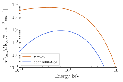
Figure 5: Solar-reflected DM flux for our benchmark points: $M_{{\rm DM}}=2\,\mathrm{MeV}$ and $\sigma_{e}=4\times 10^{-38}\,\mathrm{cm}^{2}$ in the $p$-wave case and $M_{{\rm DM}}=3\,\mathrm{MeV}$, $\sigma_{e}=1.9\times 10^{-38}\,\mathrm{cm}^{2}$ and $\delta=3\,\mathrm{keV}$ in the coannihilation case.

Once the reflected DM flux is computed, the electron recoil spectra are given by eqs. (15)–(17), with the number of the target particle taken as $N_{T}=4.2\times 10^{27}$ per tonne in our computation. As mentioned in the main text, we compute the atomic form factor following Essig et al. (2012); Bloch et al. (2020). Assuming the plane wave function for the out-going electron, the atomic form factor is given by

$$\left\lvert f_{nl}(q,E_{R})\right\rvert^{2} =F_{\mathrm{Fermi}}\frac{2l+1}{2\pi^{3}}\frac{m_{e}E_{R}}{q}\left[\int_{k_{-}}^{k_{+}}dk\,k\left\lvert\chi_{nl}\left(k\right)\right\rvert^{2}\right],$$

$$k_{\pm} =\left\lvert\sqrt{2m_{e}E_{R}}\pm q\right\rvert.$$ (34)

The radial part of the wave function in the momentum space $\chi_{nl}$ is given by

$$\chi_{nl}(k)=4\pi\int_{0}^{\infty}dr\,r^{2}j_{l}\left(kr\right)R_{nl}\left(r\right),$$ (35)

where $j_{l}$ is the spherical Bessel function and $R_{nl}$ is the radial part of the real space wave function. We take $R_{nl}$ as

$$R_{nl} =\sum_{j}C_{jln}N_{jl}r^{n_{jl}-1}\exp\left(-Z_{jl}r\right),$$

$$N_{jl} =\frac{\left(2Z_{jl}\right)^{n_{jl}+1/2}}{\sqrt{\left(2n_{jl}\right)!}}.$$ (36)

where $C_{jln},Z_{jl}$ and $n_{jl}$ are taken from Bunge et al. (1993). If we define

$$f_{l}\left(n;x\right)\equiv\frac{2^{n+1/2}}{\sqrt{\left(2n\right)!}}\int_{0}^{\infty}dy\,y^{n+1}j_{l}\left(xy\right)\exp\left(-y\right),$$ (37)

the momentum-space wave function is given by

$$\chi_{nl}\left(k\right)=4\pi\sum_{j}\frac{C_{jln}}{Z_{jl}^{3/2}}f_{l}\left(n_{jl};k/Z_{jl}\right).$$ (38)

The integral (37) can be analytically performed, which simplifies the numerical computation. The wave functions are normalized as

$$\int dk\,k^{2}\left\lvert\chi_{nl}\right\rvert^{2}=\left(2\pi\right)^{3},\quad\int_{0}^{\infty}dr\,r^{2}\left\lvert R_{nl}\right\rvert^{2}=1,$$ (39)

which agrees with the normalization of Bunge et al. (1993). Finally the Fermi factor is given by

$$F_{\mathrm{Fermi}}(q)=\frac{2\pi d}{1-e^{-2\pi d}},\quad d=Z_{\mathrm{eff}}\frac{\alpha_{e}m_{e}}{q},$$ (40)

where we take the effective charge as $Z_{\mathrm{eff}}=1$. We show the form factors without the Fermi factor in Fig. 6. They agree well with Bloch et al. (2020) except in the region $q\lesssim 10\,\mathrm{keV}$ for the $4d$-state electron with $E_{R}=1\,\mathrm{keV}$, whose effect on the final result is anyway minor. In our computation we neglect the contribution from $1s$, $2s$ and $2p$ electrons, because their binding energies are larger than $\simeq 4.8$ keV (see e.g. Bunge et al. (1993)) and thus can be neglected in this specific study. We included 8 orbits, from $3s$ up to $5p$.

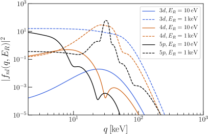
Figure 6: Atomic form factors of the $3d$-, $4d$- and $5p$-state electrons without the Fermi factor, with two different values of the recoil energy $E_{R}$.

After computing the electron recoil spectra, we convolute them with the detector response to obtain the signals. For the S2-only analysis, we use the mean values in Aprile et al. (2019) to translate the recoil energy to photoelectron (PE). Although the efficiency depends on the position of the event, we simply multiply all the efficiency shown in Aprile et al. (2019) to obtain the signals in this work. A more detailed analysis on the detector response is left as a future work. For the recent S1$+$S2 analysis, we follow the procedure outlined in the original paper Aprile et al. (2020). We smear the events by a gaussian distribution with the width given by

$$\sigma\left(E\right)=a\sqrt{E}+bE,$$ (41)

where we take $a=0.31\sqrt{\mathrm{keV}}$ and $b=0.0037$ in our numerical computation. We then multiply the efficiency that is again given in Aprile et al. (2020).

References

- Prantzos et al. (2011) N. Prantzos et al., Rev. Mod. Phys. 83, 1001 (2011), arXiv:1009.4620 [astro-ph.HE] .
- Siegert et al. (2016) T. Siegert, R. Diehl, G. Khachatryan, M. G. Krause, F. Guglielmetti, J. Greiner, A. W. Strong, and X. Zhang, Astron. Astrophys. 586, A84 (2016), arXiv:1512.00325 [astro-ph.HE] .
- Kierans et al. (2019) C. A. Kierans et al., (2019), arXiv:1912.00110 [astro-ph.HE] .
- Aprile et al. (2019) E. Aprile et al. (XENON), Phys. Rev. Lett. 123, 251801 (2019), arXiv:1907.11485 [hep-ex] .
- Aprile et al. (2020) E. Aprile et al. (XENON), (2020), arXiv:2006.09721 [hep-ex] .
- Beacom and Yuksel (2006) J. F. Beacom and H. Yuksel, Phys. Rev. Lett. 97, 071102 (2006), arXiv:astro-ph/0512411 .
- Bartels et al. (2018) R. Bartels, F. Calore, E. Storm, and C. Weniger, Mon. Not. Roy. Astron. Soc. 480, 3826 (2018), arXiv:1803.04370 [astro-ph.HE] .
- Fuller et al. (2019) G. M. Fuller, A. Kusenko, D. Radice, and V. Takhistov, Phys. Rev. Lett. 122, 121101 (2019), arXiv:1811.00133 [astro-ph.HE] .
- Boehm et al. (2004) C. Boehm, D. Hooper, J. Silk, M. Casse, and J. Paul, Phys. Rev. Lett. 92, 101301 (2004), arXiv:astro-ph/0309686 .
- Vincent et al. (2012) A. C. Vincent, P. Martin, and J. M. Cline, JCAP 04, 022 (2012), arXiv:1201.0997 [hep-ph] .
- Jia (2018) L.-B. Jia, Eur. Phys. J. C78, 112 (2018), arXiv:1710.03906 [hep-ph] .
- Wilkinson et al. (2016) R. J. Wilkinson, A. C. Vincent, C. Bœhm, and C. McCabe, Phys. Rev. D94, 103525 (2016), arXiv:1602.01114 [astro-ph.CO] .
- Escudero (2019) M. Escudero, JCAP 02, 007 (2019), arXiv:1812.05605 [hep-ph] .
- Sabti et al. (2020) N. Sabti, J. Alvey, M. Escudero, M. Fairbairn, and D. Blas, JCAP 2001, 004 (2020), arXiv:1910.01649 [hep-ph] .
- Saikawa and Shirai (2020) K. Saikawa and S. Shirai, (2020), arXiv:2005.03544 [hep-ph] .
- Valenti et al. (2018) E. Valenti, M. Zoccali, A. Mucciarelli, O. A. Gonzalez, F. Surot, D. Minniti, M. Rejkuba, L. Pasquini, G. Fiorentino, G. Bono, and et al., Astronomy & Astrophysics 616, A83 (2018), arXiv:1805.00275 [astro-ph] .
- Ascasibar et al. (2006) Y. Ascasibar, P. Jean, C. Boehm, and J. Knoedlseder, Mon. Not. Roy. Astron. Soc. 368, 1695 (2006), arXiv:astro-ph/0507142 .
- Rasera et al. (2006) Y. Rasera, R. Teyssier, P. Sizun, B. Cordier, J. Paul, M. Casse, and P. Fayet, Phys. Rev. D 73, 103518 (2006), arXiv:astro-ph/0507707 .
- Slatyer (2016) T. R. Slatyer, Phys. Rev. D 93, 023527 (2016), arXiv:1506.03811 [hep-ph] .
- Boudaud et al. (2019) M. Boudaud, T. Lacroix, M. Stref, and J. Lavalle, Phys. Rev. D 99, 061302 (2019), arXiv:1810.01680 [astro-ph.HE] .
- Ema et al. (2019) Y. Ema, F. Sala, and R. Sato, Phys. Rev. Lett. 122, 181802 (2019), arXiv:1811.00520 [hep-ph] .
- Cappiello and Beacom (2019) C. Cappiello and J. F. Beacom, Phys. Rev. D 100, 103011 (2019), arXiv:1906.11283 [hep-ph] .
- Banerjee et al. (2019) D. Banerjee et al., Phys. Rev. Lett. 123, 121801 (2019), arXiv:1906.00176 [hep-ex] .
- Åkesson et al. (2018) T. Åkesson et al. (LDMX), (2018), arXiv:1808.05219 [hep-ex] .
- Abazajian et al. (2019) K. Abazajian et al., (2019), arXiv:1907.04473 [astro-ph.IM] .
- Ade et al. (2019) P. Ade et al. (Simons Observatory), JCAP 02, 056 (2019), arXiv:1808.07445 [astro-ph.CO] .
- Krnjaic (2016) G. Krnjaic, Phys. Rev. D 94, 073009 (2016), arXiv:1512.04119 [hep-ph] .
- Dev et al. (2020) P. B. Dev, R. N. Mohapatra, and Y. Zhang, (2020), arXiv:2005.00490 [hep-ph] .
- Kolb and Turner (1990) E. W. Kolb and M. S. Turner, Front. Phys. 69, 1 (1990).
- Baryakhtar et al. (2020) M. Baryakhtar, A. Berlin, H. Liu, and N. Weiner, (2020), arXiv:2006.13918 [hep-ph] .
- Harigaya et al. (2020) K. Harigaya, Y. Nakai, and M. Suzuki, (2020), arXiv:2006.11938 [hep-ph] .
- Lee (2020) H. M. Lee, (2020), arXiv:2006.13183 [hep-ph] .
- Bramante and Song (2020) J. Bramante and N. Song, (2020), arXiv:2006.14089 [hep-ph] .
- Bloch et al. (2020) I. M. Bloch, A. Caputo, R. Essig, D. Redigolo, M. Sholapurkar, and T. Volansky, (2020), arXiv:2006.14521 [hep-ph] .
- An and Yang (2020) H. An and D. Yang, (2020), arXiv:2006.15672 [hep-ph] .
- Baek et al. (2020) S. Baek, J. Kim, and P. Ko, (2020), arXiv:2006.16876 [hep-ph] .
- He et al. (2020) H.-J. He, Y.-C. Wang, and J. Zheng, (2020), arXiv:2007.04963 [hep-ph] .
- An et al. (2018) H. An, M. Pospelov, J. Pradler, and A. Ritz, Phys. Rev. Lett. 120, 141801 (2018), [Erratum: Phys.Rev.Lett. 121, 259903 (2018)], arXiv:1708.03642 [hep-ph] .
- Bahcall et al. (2005) J. N. Bahcall, A. M. Serenelli, and S. Basu, Astrophys. J. Lett. 621, L85 (2005), arXiv:astro-ph/0412440 .
- Essig et al. (2016) R. Essig, M. Fernandez-Serra, J. Mardon, A. Soto, T. Volansky, and T.-T. Yu, JHEP 05, 046 (2016), arXiv:1509.01598 [hep-ph] .
- Essig et al. (2012) R. Essig, J. Mardon, and T. Volansky, Phys. Rev. D 85, 076007 (2012), arXiv:1108.5383 [hep-ph] .
- Roberts et al. (2016) B. Roberts, V. Dzuba, V. Flambaum, M. Pospelov, and Y. Stadnik, Phys. Rev. D 93, 115037 (2016), arXiv:1604.04559 [hep-ph] .
- Roberts and Flambaum (2019) B. Roberts and V. Flambaum, Phys. Rev. D 100, 063017 (2019), arXiv:1904.07127 [hep-ph] .
- Fu et al. (2017) C. Fu et al. (PandaX), Phys. Rev. Lett. 119, 181806 (2017), arXiv:1707.07921 [hep-ex] .
- Banerjee et al. (2018) D. Banerjee et al. (NA64), Phys. Rev. D 97, 072002 (2018), arXiv:1710.00971 [hep-ex] .
- Liu et al. (2017) Y.-S. Liu, D. McKeen, and G. A. Miller, Phys. Rev. D 95, 036010 (2017), arXiv:1609.06781 [hep-ph] .
- Liu and Miller (2017) Y.-S. Liu and G. A. Miller, Phys. Rev. D 96, 016004 (2017), arXiv:1705.01633 [hep-ph] .
- Pato et al. (2015) M. Pato, F. Iocco, and G. Bertone, JCAP 12, 001 (2015), arXiv:1504.06324 [astro-ph.GA] .
- Buch et al. (2019) J. Buch, S. C. J. Leung, and J. Fan, JCAP 04, 026 (2019), arXiv:1808.05603 [astro-ph.GA] .
- Bunge et al. (1993) C. Bunge, J. Barrientos, and A. Bunge, Atom. Data Nucl. Data Tabl. 53, 113 (1993).