Inductive construction of stable envelopes

Abstract

We revisit the construction of stable envelopes in equivariant elliptic cohomology [1] and give a direct inductive proof of their existence and uniqueness in a rather general situation. We also discuss the specialization of this construction to equivariant K-theory.

1 Introduction

1.1 Stable envelopes

1.1.1

While representation theory works with linear operators between vector spaces, the geometric representation theory works with correspondences. By definition a correspondence between, say, two smooth quasiprojective algebraic varieties $\mathsf{X}$ and $\mathsf{X}^{\prime}$ over $\mathbb{C}$ is an equivariant cohomology, or K-theory, or elliptic cohomology class on the product $\mathsf{X}\times\mathsf{X}^{\prime}$. With appropriate properness assumptions, these can be composed, and this composition is linear over the corresponding cohomology theory of a point.

While this setting is extremely general, there is one very particular class of correspondences, the stable envelopes, that has been a focus of a lot of current research, with decisive application to geometric construction of quantum groups, including elliptic quantum groups and related algebras, as well as to a number of core questions in enumerative geometry and mathematical physics, see [1, 2, MO1, Opcmi, SaltLake, Rio] for an introduction.

1.1.2

If an algebraic torus $\mathsf{A}$ acts on $\mathsf{X}$ then the fixed locus $\mathsf{X}^{\prime}=\mathsf{X}^{\mathsf{A}}$ is smooth and, moreover, there is a locally closed smooth submanifold

$$\mathsf{Attr}=\{(x,y),\lim_{a\to 0}a\cdot x=y\}\subset\mathsf{X}\times\mathsf{X}^{\mathsf{A}}$$ (1)

for any generic choice of $a\in\mathsf{A}$ going to infinity of the torus. Stable envelopes are certain canonical extension of these attracting (also known as stable) manifolds to well-defined correspondences between $\mathsf{X}^{\mathsf{A}}$ and $\mathsf{X}$.

From definitions, one easily veryfies the uniqueness of stable envelopes. Their existence, however, is far from obvious, which is a reason why they are a powerful and versatile tool.

1.1.3

A direct geometric proof of existence of stable envelopes in equivariant cohomology was given in [MO1]. That line of argument, however, is not available in equivariant K-theory and elliptic cohomology.

A very different argument for existence of stable envelopes, which is specific to $\mathsf{X}$ being a Nakajima quiver variety, or more generally a GIT quotient of a certain special form, was given in [1]. Since elliptic stable envelopes are particularly important for applications, it highly desirable to have a more general and flexible way to construct them.

1.1.4

In essense, an equivariant elliptic cohomology class on $\mathsf{X}$ is a section of a line bundle $\mathscr{S}$ on the scheme $\operatorname{Ell}_{\textup{eq}}(\mathsf{X})$, where the equivariance is with respect to some group which contains $\mathsf{A}$ in its center. Being an extension of (1) puts a numerical constraint on $\mathscr{S}$, that is, a constraint on the degree of $\mathscr{L}$. We call bundles satisfying this constraint attractive, see Definition 1.

The main result of the paper may be informally summarized as proving that elliptic stable envelopes exist, with a direct inductive construction, whenever there exist attractive line bundles for $\mathsf{X}$, see the following section for a precise list of our assumptions.

Existence of attractive line bundles is a nontrivial contraint if $\operatorname{rk}\mathsf{A}>1$. Not surprisingly, the most powerful application of stable envelopes, such as geometric construction of quantum groups, require tori of rank more than one.

1.1.5

We also give a parallel construction in equivariant K-theory and check that the two constructions agree when the elliptic curve of the elliptic cohomology theory degenerates to a nodal curve.

1.2 Assumptions

1.2.1

Let $\mathsf{X}$ be a smooth quasi-projective algebraic variety over $\mathbb{C}$ with an action of a torus $\mathsf{T}$. Since $\mathsf{X}$ is smooth, it follows, see e.g. Theorem 5.1.25 in [CG], that the action of $\mathsf{T}$ can be linearized, that is, the quasi-projective embedding $\mathsf{X}\subset\mathbb{P}(\mathbb{C}^{N})$ may be chosen $\mathsf{T}$-equivariant. We fix a subtorus $\mathsf{A}\subset\mathsf{T}$.

1.2.2

The logic of this paper does not require any assumptions about equivariant formality, tautological generation, or the vanishing of the odd cohomology of $\mathsf{X}$.

1.2.3

We require that the union of attracting manifolds for $\mathsf{A}$ is closed in $\mathsf{X}$, see Section 1.3.3.

1.2.4

Stable envelopes are improved versions of attracting manifolds (1) for the subtorus $\mathsf{A}\subset\mathsf{T}$. If $\operatorname{rk}\mathsf{A}>1$, the existence of stable envelopes puts a nontrivial constraint on the $\mathsf{A}$-action, see Section 2.1.8.

One geometrically transparent way to satisfy this constraint is to have an $\mathsf{A}$-polarization, that is, a class $T^{1/2}_{\mathsf{X}}\in K_{\mathsf{A}}(\mathsf{X})$ y such that

$$T\mathsf{X}=T^{1/2}_{\mathsf{X}}+\left(T^{1/2}_{\mathsf{X}}\right)^{\vee}\quad\textup{in $K_{\mathsf{A}}(\mathsf{X})$}\,.$$

Existence of a polarization is assumed in the definition of elliptic stable envelopes given in [1]. Here we work with weaker assumptions.

1.3 Attracting manifolds

1.3.1

The setup is the same as e.g. Section 3.2 of [MO1] or Section 3.1 of [1]. Let

$$\mathsf{X}^{\mathsf{A}}=\bigsqcup F_{i}$$

be the decomposition of the $\mathsf{A}$-fixed locus into components. Since $\mathsf{X}$ is smooth, each $F_{i}$ is smooth.

1.3.2

The $\mathsf{A}$-weights in the normal bundle $N_{\mathsf{X}/\mathsf{X}^{\mathsf{A}}}$ form a finite subset $\{w_{i}\}\subset\operatorname{char}(\mathsf{A})$. The dual hyperplanes partition the vector space

$$\operatorname{Lie}_{\mathbb{R}}\mathsf{A}=\operatorname{cochar}\mathsf{A}\otimes_{\mathbb{Z}}\mathbb{R}$$ (2)

into finitely many chambers. A choice of a chamber $\mathfrak{C}$ separates $\{w_{i}\}$ into those positive on $\mathfrak{C}$, which we call attracting, and those negative on $\mathfrak{C}$, which we call repelling. We define

$$a\to 0_{\mathfrak{C}}\quad\Leftrightarrow\quad w_{i}(a)\to\begin{cases}0\,,&\textup{$w_{i}$ is attacting}\,,\\ \infty\,,&\textup{$w_{i}$ is repelling}\,.\end{cases}$$

The point $0_{\mathfrak{C}}$ may be interpreted as a fixed point in the toric compactification $\overline{\mathsf{A}}\supset\mathsf{A}$ defined by the fan of the chambers.

1.3.3

While the ability to vary $\mathfrak{C}$ is essential in the general development of the theory, in this paper we can fix a choice of $\mathfrak{C}$ once and for all. It gives a locally closed submanifold (1). Its projection to two factors is a locally closed embedding and a fibration is affine spaces, respectively, by the classical results of [BB].

We require that the image of $\mathsf{Attr}$ in $\mathsf{X}$ is closed, cf. Section 1.2.3.

For a component $F$ of the fixed locus $\mathsf{X}^{\mathsf{A}}$, we denote by $\operatorname{Attr}(F)\subset\mathsf{X}$ its attracting manifold. This is a projection of a component of $\mathsf{Attr}$ to the first factor.

1.3.4

Since the $\mathsf{A}$-action on $\mathsf{X}$ is linearized, the set of components $\{F_{i}\}$ is partially ordered by the containment in the closure of the attracting manifolds, that is,

$$\overline{\operatorname{Attr}(F_{i})}\supset F_{j}\Rightarrow F_{i}\geq F_{j}\,.$$ (3)

Iterating taking closures and attracting manifolds produces a $\mathsf{T}$-invariant singular closed subvariety

$$\mathsf{Attr}^{f}\subset\mathsf{X}\times\mathsf{X}^{\mathsf{A}}$$ (4)

formed by the pairs $(x,y)$ that belong to a chain of closures of attracting $\mathsf{A}$-orbits. By construction, $\mathsf{Attr}^{f}\subset\mathsf{Attr}^{\leq}$, where

$$\mathsf{Attr}^{\leq}=\bigcup_{F_{j}\leq F_{i}}\operatorname{Attr}(F_{j})\times F_{i}\,.$$ (5)

1.3.5

Stable envelopes are certain canonical $\mathsf{T}$-equivariant correspondences supported on $\mathsf{Attr}^{f}$. Their exact flavor depends on the chosen cohomology theory. The main focus in this paper is on stable envelopes in equivariant elliptic cohomology, as defined in [1].

1.3.6

The main aspect in which elliptic cohomology differs from equivariant cohomology ${H}^{\raisebox{1.42262pt}{$\scriptscriptstyle\bullet$}}_{\mathsf{T}}(\mathsf{X})$ or equivariant K-theory $K_{\mathsf{T}}(\mathsf{X})$ is the following. While cohomology classes form a supercommutative ring, one doesn’t tend to think about them as functions on $\operatorname{Spec}{H}^{\raisebox{1.42262pt}{$\scriptscriptstyle\bullet$}}_{\mathsf{T}}(\mathsf{X})$. In elliptic theory, $\operatorname{Spec}{H}^{\raisebox{1.42262pt}{$\scriptscriptstyle\bullet$}}_{\mathsf{T}}(\mathsf{X})$ is promoted to a superscheme

$$(\operatorname{Spec}{H}^{\raisebox{1.42262pt}{$\scriptscriptstyle\bullet$}}_{\mathsf{T}}(\mathsf{X}),{H}^{\raisebox{1.42262pt}{$\scriptscriptstyle\bullet$}}_{\mathsf{T}}(\mathsf{X}))\rightsquigarrow(\operatorname{Ell}_{\mathsf{T}}(\mathsf{X}),{\mathscr{O}}^{\raisebox{1.42262pt}{$\scriptscriptstyle\bullet$}}_{\operatorname{Ell}_{\mathsf{T}}(\mathsf{X})})\,,$$

which is no longer affine. As a result, global sections of ${\mathscr{O}}^{\raisebox{1.42262pt}{$\scriptscriptstyle\bullet$}}_{\operatorname{Ell}_{\mathsf{T}}(\mathsf{X})}$ are not rich enough to account for the geometry of $\mathsf{T}$ and $\mathsf{X}$.

In a nutshell, elliptic cohomology classes are sections of line bundles on $\operatorname{Ell}_{\mathsf{T}}(\mathsf{X})$. In particular, the elliptic stable envelopes are global sections of certain line bundles on $\operatorname{Ell}_{\mathsf{T}}(\mathsf{X}\times\mathsf{X}^{\mathsf{A}})$. We note that the very existence of the required line bundles puts a nontrivial constraint on the $\mathsf{A}$-action on $\mathsf{X}$, see Section 2.1.8.

1.4 Equivariant elliptic cohomology

1.4.1

Let $E$ be an elliptic curve over a Noetherian affine base scheme $\mathsf{B}$. For the purposes of this paper, one doesn’t loose or gain much if one assumes that $\mathsf{B}=\operatorname{Spec}\mathbb{C}$ or $\mathsf{B}=\operatorname{Spec}\mathbb{C}(\!(q)\!)$. Since elliptic stable envelopes are unique without invoking any equivalence relations, their construction is local over the base scheme.

1.4.2

Let $\mathsf{G}$ be a compact Lie group. Equivariant elliptic cohomology, developed in [Groj, 13, Rosu, Lurie, Gepner, Ganter] and other papers, defines a functor

$$\operatorname{Ell}_{\mathsf{G}}(\mathsf{X},\partial\mathsf{X}):\big{\{}\textup{pairs of $\mathsf{G}$-spaces}\big{\}}\to\{\textup{graded superschemes over $\mathsf{B}$}\}\,,$$ (6)

covariant with respect to action-preserving maps

$$f:(\mathsf{G}_{1},\mathsf{X}_{1},\partial\mathsf{X}_{1})\to(\mathsf{G}_{2},\mathsf{X}_{2},\partial\mathsf{X}_{2})\,\,.$$ (7)

In this paper, we stay entirely in the world of unitary and abelian groups $\mathsf{G}$. We assume that $E$ is such that the functor (6) has been defined.

For $\mathsf{G}$ connected, we denote the split reductive group over $\mathbb{Z}$ corresponding to $\mathsf{G}$ by the same symbol $\mathsf{G}$. With this convention, we can talk about both the $\mathsf{A}$-attracting manifolds and $\mathsf{A}$-equivariant elliptic cohomology without overloading the notation.

We abbreviate $\operatorname{Ell}_{\mathsf{G}}(\mathsf{X},\partial\mathsf{X})$ to $\operatorname{Ell}_{\mathsf{G}}(\mathsf{X})$ when $\partial\mathsf{X}=\varnothing$.

1.4.3

To save on notation for functorial maps, we abbreviate $\operatorname{Ell}(f)$ to just $f$ in what follows. We use $f^{*}$ and $f_{*}$ to denote pullback of coherent sheaves under $\operatorname{Ell}(f)$. Note the crucial difference between $f_{*}$ and push-forward in elliptic cohomology, see Section A.3.1.

1.4.4

The grading in (6) refers to the $\mathbb{Z}$-grading of the structure sheaf

$${\mathscr{O}}^{\raisebox{1.42262pt}{$\scriptscriptstyle\bullet$}}_{\operatorname{Ell}_{\mathsf{G}}(\mathsf{X})}=\bigoplus_{k\in\mathbb{Z}}\mathscr{O}^{k}_{\operatorname{Ell}_{\mathsf{G}}(\mathsf{X})}$$ (8)

of $\operatorname{Ell}_{\mathsf{T}}(\mathsf{X})$. Periodicity in elliptic cohomology means that

$$\mathscr{O}^{k-2}_{\operatorname{Ell}_{\mathsf{G}}(\mathsf{X})}=\mathscr{O}^{k}_{\operatorname{Ell}_{\mathsf{G}}(\mathsf{X})}\otimes\omega\,,\quad\omega=T^{*}_{\textup{origin}}E\,,$$

where $\omega$ is a line bundle pulled back from the base $\mathsf{B}$. This can be interpreted as having the whole theory not over $\mathsf{B}$ but over the total space of a $\mathbb{G}_{\mathbf{m}}$-bundle associated to $\omega$.

1.4.5

Line bundles $\mathscr{L}$ on $\operatorname{Ell}_{\mathsf{G}}(\mathsf{X})$ will be, by definition, graded, that is, we set

$$\operatorname{Pic}(\operatorname{Ell}_{\mathsf{G}}(\mathsf{X}))=H^{1}\left(\left(\mathscr{O}^{0}_{\operatorname{Ell}_{\mathsf{G}}(\mathsf{X})}\right)^{\times}\right)\,.$$ (9)

These can be interpreted as invertible graded ${\mathscr{O}}^{\raisebox{1.42262pt}{$\scriptscriptstyle\bullet$}}_{\operatorname{Ell}_{\mathsf{G}}(\mathsf{X})}$-bimodules and they form a commutative group with respect to $\otimes$.

1.4.6

Stable envelopes are even classes and $\mathscr{O}^{k}_{\operatorname{Ell}_{\mathsf{G}}(\mathsf{X})}$ with $k\neq 0$ will not play an important role in this paper. For brevity, we will suppress the degree grading from our notation, except where it essential (which happens in the analysis of the long exact sequence in Section 2.5).

1.4.7

By construction,

$$\operatorname{Ell}_{\mathbb{C}^{\times}}(\operatorname{pt})=E$$

and

$$\lx@xy@svg{\hbox{\raise 0.0pt\hbox{\kern 28.70837pt\hbox{\ignorespaces\ignorespaces\ignorespaces\hbox{\vtop{\kern 0.0pt\offinterlineskip\halign{\entry@#!@&&\entry@@#!@\cr&&&\\&&&\crcr}}}\ignorespaces{\hbox{\kern-18.46669pt\raise 0.0pt\hbox{\hbox{\kern 0.0pt\raise 0.0pt\hbox{\hbox{\kern 3.0pt\raise 0.0pt\hbox{$\textstyle{\mathbb{C}^{\times}\times\mathbb{C}^{\times}\ignorespaces\ignorespaces\ignorespaces\ignorespaces\ignorespaces\ignorespaces\ignorespaces\ignorespaces}$}}}}}}}\ignorespaces\ignorespaces\ignorespaces\ignorespaces{}{\hbox{\lx@xy@droprule}}\ignorespaces\ignorespaces\ignorespaces{\hbox{\kern 36.05695pt\raise 6.5pt\hbox{{}\hbox{\kern 0.0pt\raise 0.0pt\hbox{\hbox{\kern 3.0pt\hbox{\hbox{\kern 0.0pt\raise-1.75pt\hbox{$\scriptstyle{(z_{1},z_{2})\to z_{1}z_{2}}$}}}\kern 3.0pt}}}}}}\ignorespaces{\hbox{\kern 102.46669pt\raise 0.0pt\hbox{\hbox{\kern 0.0pt\raise 0.0pt\hbox{\lx@xy@tip{1}\lx@xy@tip{-1}}}}}}{\hbox{\lx@xy@droprule}}{\hbox{\lx@xy@droprule}}\ignorespaces\ignorespaces\ignorespaces\ignorespaces{}{\hbox{\lx@xy@droprule}}\ignorespaces\ignorespaces\ignorespaces{\hbox{\kern-28.70837pt\raise-19.25554pt\hbox{{}\hbox{\kern 0.0pt\raise 0.0pt\hbox{\hbox{\kern 3.0pt\hbox{\hbox{\kern 0.0pt\raise-1.75pt\hbox{$\scriptstyle{\operatorname{Ell}_{\bullet}(\operatorname{pt})}$}}}\kern 3.0pt}}}}}}\ignorespaces{\hbox{\kern 0.0pt\raise-28.67776pt\hbox{\hbox{\kern 0.0pt\raise 0.0pt\hbox{\lx@xy@tip{1}\lx@xy@tip{-1}}}}}}{\hbox{\lx@xy@droprule}}{\hbox{\lx@xy@droprule}}{\hbox{\kern 42.46669pt\raise 0.0pt\hbox{\hbox{\kern 0.0pt\raise 0.0pt\hbox{\hbox{\kern 3.0pt\raise 0.0pt\hbox{$\textstyle{}$}}}}}}}{\hbox{\kern 72.46669pt\raise 0.0pt\hbox{\hbox{\kern 0.0pt\raise 0.0pt\hbox{\hbox{\kern 3.0pt\raise 0.0pt\hbox{$\textstyle{}$}}}}}}}{\hbox{\kern 102.46669pt\raise 0.0pt\hbox{\hbox{\kern 0.0pt\raise 0.0pt\hbox{\hbox{\kern 3.0pt\raise 0.0pt\hbox{$\textstyle{\mathbb{C}^{\times}\ignorespaces\ignorespaces\ignorespaces\ignorespaces}$}}}}}}}\ignorespaces\ignorespaces\ignorespaces\ignorespaces{}{\hbox{\lx@xy@droprule}}\ignorespaces\ignorespaces\ignorespaces{\hbox{\kern 111.25558pt\raise-19.25554pt\hbox{{}\hbox{\kern 0.0pt\raise 0.0pt\hbox{\hbox{\kern 3.0pt\hbox{\hbox{\kern 0.0pt\raise-1.75pt\hbox{$\scriptstyle{\operatorname{Ell}_{\bullet}(\operatorname{pt})}$}}}\kern 3.0pt}}}}}}\ignorespaces{\hbox{\kern 111.25558pt\raise-28.67776pt\hbox{\hbox{\kern 0.0pt\raise 0.0pt\hbox{\lx@xy@tip{1}\lx@xy@tip{-1}}}}}}{\hbox{\lx@xy@droprule}}{\hbox{\lx@xy@droprule}}{\hbox{\kern-17.06938pt\raise-38.51108pt\hbox{\hbox{\kern 0.0pt\raise 0.0pt\hbox{\hbox{\kern 3.0pt\raise 0.0pt\hbox{$\textstyle{E\times E\ignorespaces\ignorespaces\ignorespaces\ignorespaces}$}}}}}}}\ignorespaces\ignorespaces\ignorespaces\ignorespaces{}{\hbox{\lx@xy@droprule}}\ignorespaces\ignorespaces\ignorespaces{\hbox{\kern 37.54861pt\raise-32.39998pt\hbox{{}\hbox{\kern 0.0pt\raise 0.0pt\hbox{\hbox{\kern 3.0pt\hbox{\hbox{\kern 0.0pt\raise-1.75pt\hbox{$\scriptstyle{\textup{group law}}$}}}\kern 3.0pt}}}}}}\ignorespaces{\hbox{\kern 104.27643pt\raise-38.51108pt\hbox{\hbox{\kern 0.0pt\raise 0.0pt\hbox{\lx@xy@tip{1}\lx@xy@tip{-1}}}}}}{\hbox{\lx@xy@droprule}}{\hbox{\lx@xy@droprule}}{\hbox{\kern 42.46669pt\raise-38.51108pt\hbox{\hbox{\kern 0.0pt\raise 0.0pt\hbox{\hbox{\kern 3.0pt\raise 0.0pt\hbox{$\textstyle{}$}}}}}}}{\hbox{\kern 72.46669pt\raise-38.51108pt\hbox{\hbox{\kern 0.0pt\raise 0.0pt\hbox{\hbox{\kern 3.0pt\raise 0.0pt\hbox{$\textstyle{}$}}}}}}}{\hbox{\kern 104.27643pt\raise-38.51108pt\hbox{\hbox{\kern 0.0pt\raise 0.0pt\hbox{\hbox{\kern 3.0pt\raise 0.0pt\hbox{$\textstyle{E}$}}}}}}}\ignorespaces}}}}\ignorespaces\,. \textstyle{\mathbb{C}^{\times}\times\mathbb{C}^{\times}\ignorespaces\ignorespaces\ignorespaces\ignorespaces\ignorespaces\ignorespaces\ignorespaces\ignorespaces} \scriptstyle{(z_{1},z_{2})\to z_{1}z_{2}} \scriptstyle{\operatorname{Ell}_{\bullet}(\operatorname{pt})} \textstyle{\mathbb{C}^{\times}\ignorespaces\ignorespaces\ignorespaces\ignorespaces} \scriptstyle{\operatorname{Ell}_{\bullet}(\operatorname{pt})} \textstyle{E\times E\ignorespaces\ignorespaces\ignorespaces\ignorespaces} \textstyle{E} \textstyle{\mathbb{C}^{\times}\times\mathbb{C}^{\times}\ignorespaces\ignorespaces\ignorespaces\ignorespaces\ignorespaces\ignorespaces\ignorespaces\ignorespaces} \scriptstyle{(z_{1},z_{2})\to z_{1}z_{2}} \scriptstyle{\operatorname{Ell}_{\bullet}(\operatorname{pt})} \textstyle{\mathbb{C}^{\times}\ignorespaces\ignorespaces\ignorespaces\ignorespaces} \scriptstyle{\operatorname{Ell}_{\bullet}(\operatorname{pt})} \textstyle{E\times E\ignorespaces\ignorespaces\ignorespaces\ignorespaces} \textstyle{E}$$ (10)

One can treat the coordinate on $\mathbb{C}^{\times}$ is a stand-in for the unavailable coordinate on $E$. If fact, for $\mathsf{B}=\operatorname{Spec}\mathbb{C}$ one can take $E=\mathbb{C}^{\times}/q^{\mathbb{Z}}$ for some $|q|<1$.

1.4.8

The map to the point

$$p_{\mathsf{X}}:(\mathsf{T},\mathsf{X})\to(\mathsf{T},\operatorname{pt})$$ (11)

makes $\operatorname{Ell}_{\mathsf{T}}(\mathsf{X})$ a scheme over

$$\mathscr{E}_{\mathsf{T}}\overset{\tiny\textup{def}}{=}\operatorname{Ell}_{\mathsf{T}}(\operatorname{pt})=\operatorname{cochar}(\mathsf{T})\otimes_{\mathbb{Z}}E\,.$$ (12)

1.4.9

We will be using various constructions in elliptic cohomology which are reviewed in Appendix A.

1.5 Plan of the paper and acknowledgments

1.5.1

The three main sections of the paper are devoted to: (1) the proof of existence and uniqueness of stable envelopes in equivariant elliptic cohomology, (2) same in equivariant K-theory, (3) the relation between the two construction.

Elliptic cohomology meets K-theory when the underlying elliptic curve degenerates to a nodal curve of genus $1$. We prove that this degeneration respects stable envelopes, strengthening earlier results of [1, 17]. Perhaps the reader will find some independent use for the notions of compactified K-theory and nodal K-theory which we develop in the course of the proof.

1.5.2

Further applications of the inductive construction of stable envelopes will be given in [24].

1.5.3

The present paper grew our of the author’s joint projects [1, 16] with Mina Aganagic, Davesh Maulik, and Daniel Halpern-Leistner. It owes a lot to all of them. While, perhaps, we achieve a certain progress on a number of technical points in this paper, the reader should consult [1, 16] as well as perhaps [MO1, Opcmi, 2] for a comprehensive discussion of stable envelopes and their many applications.

1.5.4

I am very grateful to V. Alexeev, R. Bezrukavnikov, B. Bhatt, A. Blumberg, J. de Jong, I. Krichever, M. Mustata, B. Poonen, E. Rains, R. Rouquier, D. Sinha, and others for valuable correspondence during the writing of this paper.

1.5.5

I am grateful to the Simons Foundation for being supported as a Simons Investigator. I thank the Russian Science Foundation for the support by the grant 19-11-00275.

1.6 Dedication

This paper was written in the summer of 2020, the time of great grief and loss for millions of people around the globe. I would like to dedicate it to the memory of Boris Dubrovin, whose untimely passing back in March 2019 was such a great loss for the mathematics as a whole and for me personally.

I grew up reading his Modern Geometry, and I cherish the memories of our, regrettably, infrequent interactions later in life. He always radiated enthusiasm for geometry, mathematics, music (I might have met him more often in the Moscow Conservatory than at the Moscow State University), and life and general. His pioneering vision put enumerative geometry in the front and center of modern geometry and mathematical physics. I wish I could explain the results of this paper to him.

2 Elliptic stable envelopes

2.1 Attracting manifolds again

2.1.1

Let $F$ be a component of the fixed locus $\mathsf{X}^{\mathsf{A}}$ and consider the diagram

(13)

in which $\iota$ and $\jmath$ are inclusions, $\mathsf{p}_{1}$ and $\mathsf{p}_{2}$ are projections as in (92), and

$$\pi=\mathsf{p}_{2}\,\jmath$$

is a fibration in affine spaces, and thus a homotopy equivalence. In particular,

$$\pi:\operatorname{Ell}_{\mathsf{T}}(\operatorname{Attr}(F))\xrightarrow{\quad\sim\quad}\operatorname{Ell}_{\mathsf{T}}(F)\,,$$

is an isomorphism.

2.1.2

Restricted to $F$, any $\mathsf{A}$-equivariant K-theory class decomposes according to the characters of $\mathsf{A}$ and, in particular, splits into attracting, repelling, and $\mathsf{A}$-fixed directions. For instance, we have

$$T\mathsf{X}\big{|}_{F}=N_{\mathsf{X}/F,>0}+N_{\mathsf{X}/F,<0}+TF\,,$$ (14)

where the subscripts $>0$ and $<0$ indicate the attracting and repelling directions, respectively. With this notation, we have

$$N_{\jmath}=\pi^{*}(TF+N_{\mathsf{X}/F,<0})\,,$$ (15)

where $N_{j}$ is the normal bundle to the inclusion $\jmath$ in (13).

2.1.3

Recall we think of sections of line bundles $\mathscr{L}$ on $\operatorname{Ell}_{\mathsf{T}}(\mathsf{X})$ as elliptic cohomology classes assigned to cycles in $X$. For instance, if we have a proper complex oriented map

$$f:Y\to X$$

and there is a bundle $V$ on $X$ such that $f^{*}V=N_{f}$ then $f_{{\circledast}}$ induces a section

$$\mathscr{O}_{\mathscr{E}_{\mathsf{T}}}\to\Theta(V)$$

which represents in elliptic cohomology what we would call $f_{*}[Y]\in{H}^{\raisebox{1.42262pt}{$\scriptscriptstyle\bullet$}}_{\mathsf{T}}(\mathsf{X})$. For example, the inclusion $\operatorname{pt}\to\mathsf{X}$ of a fixed point gives a section of $\mathscr{L}=\Theta(T\mathsf{X})$, while the constant section of $\mathscr{L}=\mathscr{O}_{\operatorname{Ell}_{\mathsf{T}}(\mathsf{X})}$ corresponds to the identity map $\mathsf{X}\to\mathsf{X}$ .

The degree

$$\deg\mathscr{L}\in\operatorname{Pic}(\operatorname{Ell}_{\mathsf{T}}(\mathsf{X}))\big{/}\operatorname{Pic}_{0}(\operatorname{Ell}_{\mathsf{T}}(\mathsf{X}))$$

gives a measure of the codimension of the corresponding cycle. In particular, the degree $\deg_{\mathsf{A}}\mathscr{L}$ in equivariant variables as defined in (84) is a coarse measure of the codimension.

2.1.4

Since we are looking for a line bundle $\mathscr{S}$ to represent attracting manifolds, it is logical to make the following

Definition 1.

A line bundle $\mathscr{S}$ on $\operatorname{Ell}_{\mathsf{T}}(\mathsf{X})$ is called attractive for a given choice $\mathfrak{C}$ of attracting directions if

$$\deg_{\mathsf{A}}\mathscr{S}=\deg_{\mathsf{A}}\Theta(N_{\mathsf{X}/\mathsf{X}^{\mathsf{A}},<0})\,.$$ (16)

For a given line bundle $\mathscr{S}$ on $\operatorname{Ell}_{\mathsf{T}}(\mathsf{X})$ we define

$$\mathscr{S}_{\mathsf{A}}=\iota^{*}\mathscr{S}\otimes\Theta(-N_{\mathsf{X}/\mathsf{X}^{\mathsf{A}},<0})\in\operatorname{Pic}(\operatorname{Ell}_{\mathsf{T}}(\mathsf{X}^{\mathsf{A}}))\,.$$ (17)

Clearly, (16) is equivalent to $\deg_{\mathsf{A}}\mathscr{S}_{\mathsf{A}}=0$. Also, all attractive bundles form a principal homogenous space under

$$\operatorname{Ker}\deg_{\mathsf{A}}\subset\operatorname{Pic}(\operatorname{Ell}_{\mathsf{T}}(\mathsf{X}))\,,$$

which contains all Kähler line bundles.

2.1.5

Lemma 2.1.

If $\mathscr{S}$ is attractive and $\jmath$ in (13) is proper, then $\jmath_{{\circledast}}$ gives a section

$$[\mathsf{Attr}]:\mathscr{O}_{\mathscr{E}_{\mathsf{T}}}\to\mathscr{S}\boxtimes\left(\mathscr{S}_{\mathsf{A}}\right)^{\triangledown}\,.$$ (18)

Recall that $\boxtimes$ denotes the tensor product of pullbacks via two projection maps, here $\mathsf{p}_{1}$ and $\mathsf{p}_{2}$. Also note that the duality $(\,\cdot\,)^{\triangledown}$, which was defined in (88), is applied here in the $\mathsf{X}^{\mathsf{A}}$ factor.

Proof.

Note that the outer square in (13) commutes up to homotopy

$$\mathsf{p}_{1}\,\jmath\sim\iota\,\pi\,.$$ (19)

Therefore

$$\jmath^{*}\mathsf{p}_{1}^{*}\mathscr{S}=\pi^{*}\iota^{*}\mathscr{S}$$

and

$$\jmath^{*}\left(\mathscr{S}\boxtimes\left(\mathscr{S}_{\mathsf{A}}\right)^{\triangledown}\right)=\Theta(\pi^{*}(TF+N_{X/F}))=\Theta(N_{\jmath})\,,$$

as required. ∎

2.1.6

From (14), we observe the following

Lemma 2.2.

If $\mathscr{S}$ is attractive for $\mathfrak{C}$ then $\mathscr{S}^{\triangledown}$ is attractive for $-\mathfrak{C}$.

2.1.7

It is an interesting question to characterize $\mathsf{A}$-actions having attractive line bundles. In general, the functor

$$(\mathsf{G},\mathsf{X})\to{H}^{\raisebox{1.42262pt}{$\scriptscriptstyle\bullet$}}\left(\left(\mathscr{O}^{0}_{\operatorname{Ell}_{\mathsf{G}}(\mathsf{X})}\right)^{\times}\right)\,.$$ (20)

that generalizes (9) is an interesting functor to complexes of abelian groups.

2.1.8

Simple examples, starting with the the maximal torus $\mathsf{A}\subset PGL(3)$ acting on $\mathbb{P}^{2}$, show that attracting line bundles $\mathscr{S}$ typically do not exist if $\operatorname{rk}\mathsf{A}>1$. In fact, any subtorus $\mathsf{A}^{\prime}\subset\mathsf{A}$ gives the following potential obstruction to the existence of attracting bundles in the style of [14].

Proposition 2.3.

Let $F_{1}$ and $F_{2}$ be two components of $\mathsf{X}^{\mathsf{A}}$ that belong to the same component of $X^{\mathsf{A}^{\prime}}$ where $\mathsf{A}^{\prime}\subset\mathsf{A}$ is a subtorus. If

$$\deg_{\mathsf{A}/\mathsf{A}^{\prime}}\Theta(N_{\mathsf{X}/F_{1},<0})\neq\deg_{\mathsf{A}/\mathsf{A}^{\prime}}\Theta(N_{\mathsf{X}/F_{2},<0})$$

then no attractive bundle $\mathscr{S}$ exists.

A simple way to guarantee the existence of $\mathscr{S}$ is to assume that $X$ has a polarization.

2.2 Polarization and dynamical shifts

2.2.1

By definition, a polarization of $\mathsf{X}$ with respect to $\mathsf{A}$ is a class $T^{1/2}_{\mathsf{X}}\in K_{\mathsf{A}}(\mathsf{X})$ such that

$$T\mathsf{X}=T^{1/2}_{\mathsf{X}}+\left(T^{1/2}_{\mathsf{X}}\right)^{\vee}$$ (21)

in $K_{\mathsf{A}}(\mathsf{X})$. The existence of a polarization implies, in particular, that $\dim\mathsf{X}$ is even. Like any $\mathsf{A}$-equivariant K-theory class, $T^{1/2}_{\mathsf{X}}$ may be lifted to a $\mathsf{T}$-equivariant class so that (21) holds modulo

$$\mathscr{I}_{\mathsf{A}}=\textup{ideal of $\mathsf{A}$}\subset K_{\mathsf{T}}(\operatorname{pt})\,.$$

2.2.2 Example

Suppose we have a $\mathsf{T}$-equivariant diagram

$$\lx@xy@svg{\hbox{\raise 0.0pt\hbox{\kern 6.75pt\hbox{\ignorespaces\ignorespaces\ignorespaces\hbox{\vtop{\kern 0.0pt\offinterlineskip\halign{\entry@#!@&&\entry@@#!@\cr&&\\&&\crcr}}}\ignorespaces{\hbox{\kern-6.75pt\raise 0.0pt\hbox{\hbox{\kern 0.0pt\raise 0.0pt\hbox{\hbox{\kern 3.0pt\raise 0.0pt\hbox{$\textstyle{\mathsf{X}\ignorespaces\ignorespaces\ignorespaces\ignorespaces\ignorespaces\ignorespaces\ignorespaces\ignorespaces}$}}}}}}}\ignorespaces\ignorespaces\ignorespaces\ignorespaces{}{\hbox{\lx@xy@droprule}}\ignorespaces\ignorespaces\ignorespaces{\hbox{\kern 26.78938pt\raise 5.1875pt\hbox{{}\hbox{\kern 0.0pt\raise 0.0pt\hbox{\hbox{\kern 3.0pt\hbox{\hbox{\kern 0.0pt\raise-0.8264pt\hbox{$\scriptstyle{\textup{open}}$}}}\kern 3.0pt}}}}}}\ignorespaces{\hbox{\kern 60.75pt\raise 0.0pt\hbox{\hbox{\kern 0.0pt\raise 0.0pt\hbox{\lx@xy@tip{1}\lx@xy@tip{-1}}}}}}{\hbox{\lx@xy@droprule}}{\hbox{\lx@xy@droprule}}\ignorespaces\ignorespaces\ignorespaces{}\ignorespaces\ignorespaces{\hbox{\lx@xy@drawline@}}\ignorespaces\ignorespaces\ignorespaces{\hbox{\kern 29.91177pt\raise-23.92982pt\hbox{{}\hbox{\kern 0.0pt\raise 0.0pt\hbox{\hbox{\kern 3.0pt\hbox{\hbox{\kern 0.0pt\raise-0.8264pt\hbox{$\scriptstyle{p}$}}}\kern 3.0pt}}}}}}\ignorespaces{\hbox{\kern 65.76633pt\raise-33.24579pt\hbox{\hbox{\kern 0.0pt\raise 0.0pt\hbox{\lx@xy@tip{1}\lx@xy@tip{-1}}}}}}\ignorespaces\ignorespaces{\hbox{\lx@xy@drawline@}}\ignorespaces{\hbox{\lx@xy@drawline@}}{\hbox{\kern 30.75pt\raise 0.0pt\hbox{\hbox{\kern 0.0pt\raise 0.0pt\hbox{\hbox{\kern 3.0pt\raise 0.0pt\hbox{$\textstyle{}$}}}}}}}{\hbox{\kern 60.75pt\raise 0.0pt\hbox{\hbox{\kern 0.0pt\raise 0.0pt\hbox{\hbox{\kern 3.0pt\raise 0.0pt\hbox{$\textstyle{T^{*}M\ignorespaces\ignorespaces\ignorespaces\ignorespaces}$}}}}}}}\ignorespaces\ignorespaces\ignorespaces\ignorespaces{}{\hbox{\lx@xy@droprule}}\ignorespaces{\hbox{\kern 74.16216pt\raise-27.65138pt\hbox{\hbox{\kern 0.0pt\raise 0.0pt\hbox{\lx@xy@tip{1}\lx@xy@tip{-1}}}}}}{\hbox{\lx@xy@droprule}}{\hbox{\lx@xy@droprule}}{\hbox{\kern-3.0pt\raise-37.4847pt\hbox{\hbox{\kern 0.0pt\raise 0.0pt\hbox{\hbox{\kern 3.0pt\raise 0.0pt\hbox{$\textstyle{}$}}}}}}}{\hbox{\kern 30.75pt\raise-37.4847pt\hbox{\hbox{\kern 0.0pt\raise 0.0pt\hbox{\hbox{\kern 3.0pt\raise 0.0pt\hbox{$\textstyle{}$}}}}}}}{\hbox{\kern 65.76633pt\raise-37.4847pt\hbox{\hbox{\kern 0.0pt\raise 0.0pt\hbox{\hbox{\kern 3.0pt\raise 0.0pt\hbox{$\textstyle{M}$}}}}}}}\ignorespaces}}}}\ignorespaces\,. \textstyle{\mathsf{X}\ignorespaces\ignorespaces\ignorespaces\ignorespaces\ignorespaces\ignorespaces\ignorespaces\ignorespaces} \scriptstyle{p} \textstyle{T^{*}M\ignorespaces\ignorespaces\ignorespaces\ignorespaces} \textstyle{M} \textstyle{\mathsf{X}\ignorespaces\ignorespaces\ignorespaces\ignorespaces\ignorespaces\ignorespaces\ignorespaces\ignorespaces} \scriptstyle{p} \textstyle{T^{*}M\ignorespaces\ignorespaces\ignorespaces\ignorespaces} \textstyle{M}$$ (22)

Then either $\operatorname{Ker}(dp)$ or $p^{*}TM$ give a polarization with respect to

$$\mathsf{A}=\mathsf{T}\cap\operatorname{Aut}(\mathsf{X},\omega)\,,$$

where $\omega$ is the canonical symplectic form.

The base $M$ in (22) may be a quotient stack, and Nakajima quiver varieties [Nak1] are constructed as $\mathsf{X}$ of this form. Recall that Nakajima varieties and closely related algebraic varieties are among the most important objects in geometric representation theory. In fact, stable envelopes give one geometric approach to extracting representation theory from them, see [MO1, Opcmi] for an introduction.

2.2.3

Proposition 2.4.

If $T^{1/2}$ is a polarization then $\mathscr{S}=\Theta(T^{1/2})$ is attractive for any $\mathfrak{C}$.

Proof.

From (21) and (14) we conclude

$$N_{\mathsf{X}/\mathsf{X}^{\mathsf{A}},<0}=T^{1/2}_{<0}+\left(T^{1/2}_{>0}\right)^{\vee}+\boldsymbol{\delta\upsilon}\,,\quad\boldsymbol{\delta\upsilon}\in\mathscr{I}_{\mathsf{A}}\,K_{\mathsf{T}}(\mathsf{X}^{\mathsf{A}})\,,$$ (23)

where $T^{1/2}_{\gtrless 0}$ denote the attracting and repelling parts of $T^{1/2}\big{|}_{\mathsf{X}^{\mathsf{A}}}$. The equality (80) and

$$\deg_{\mathsf{A}}\Theta(\boldsymbol{\delta\upsilon})=0$$

prove the claim. ∎

2.2.4

The K-theory class $\boldsymbol{\delta\upsilon}$ depends on the choice of $\mathfrak{C}$, that is, on the choice of the attracting directions. In this sense it is dynamic. It also corresponds to the dynamical variables in the elliptic quantum groups, see [1]. Dynamical is a Greek word which starts with $\delta$ and $\upsilon$, the notation $\boldsymbol{\delta\upsilon}$ is chosen to reflect this.

2.2.5

When one starts composing elliptic stable envelopes, then the following formula is useful:

$$\mathscr{S}=\Theta(T^{1/2}_{\mathsf{X}})\quad\Rightarrow\quad\mathscr{S}_{\mathsf{A}}=\Theta(T^{1/2}_{\mathsf{X}^{\mathsf{A}}})\otimes\Theta(-\boldsymbol{\delta\upsilon})\,.$$ (24)

Thus the twist by $\Theta(\boldsymbol{\delta\upsilon})$ becomes the dynamical shift which is an important phenomenon in the theory of elliptic quantum group. To set it up correctly, it is useful to have the following formula for $\Theta(\boldsymbol{\delta\upsilon})$ in terms of the Kähler line bundles.

Let $\{t_{i}\}\subset\operatorname{char}(\mathsf{T}/\mathsf{A})$ be a set of coordinates on $\mathsf{T}/\mathsf{A}$. By hypothesis, there exist nonunique $\upsilon_{i}\in K_{\mathsf{T}}(\mathsf{X}^{\mathsf{A}})$ such that

$$\boldsymbol{\delta\upsilon}=\sum(t_{i}-1)\upsilon_{i}\,.$$

Therefore

$$\Theta(\boldsymbol{\delta\upsilon})=\Theta(-{\textstyle\sum}\,t_{i}\operatorname{rk}\upsilon_{i})\otimes\bigotimes\mathscr{U}(\upsilon_{i},t_{i})\,.$$ (25)

For our purposes in this paper it is not important to unpack the bundle $\Theta(\boldsymbol{\delta\upsilon})$.

2.2.6 Example

Let $\mathsf{X}=T^{*}\mathbb{P}(\mathbb{C}^{n})$ with the action of $GL(n)\times\mathbb{C}^{\times}$, where $\hbar\in\mathbb{C}^{\times}$ scales the cotangent fibers with weight $\hbar^{-1}$. Let

$$\mathsf{A}=\operatorname{diag}(a_{1},\dots,a_{n})\subset GL(n)\,,$$

be a maximal torus and choose $\mathfrak{C}$ so that

$$a\to 0_{\mathfrak{C}}\Leftrightarrow\forall i,\,a_{i}/a_{i+1}\to 0\,.$$

We take the pullback of $T_{\mathbb{P}(\mathbb{C}^{n})}$ as the polarization of $\mathsf{X}$.

The fixed locus $\mathsf{X}^{\mathsf{A}}=\sqcup F_{k}$ consists of $n$ isolated points — coordinate lines in $\mathbb{C}^{n}$. They are ordered as follows

$$F_{1}<F_{2}<\dots<F_{n}$$

in the sense that each $F_{i}$ lies in the closure of the attracting manifold of $F_{i+1}$.

The restriction of the tangent bundle to $k$-th point has the character

$$T\mathsf{X}\big{|}_{F_{k}}=\sum_{i\neq k}\left(\frac{a_{i}}{a_{k}}+\frac{a_{k}}{\hbar a_{i}}\right)\,,$$

in which the terms without $\hbar$ give the polarization. Therefore

$$\boldsymbol{\delta\upsilon}\big{|}_{F_{k}}=(\hbar^{-1}-1)\sum_{i<k}\frac{a_{k}}{a_{i}}\,.$$

Other choices of $\mathfrak{C}$ will give a different order $>_{\mathfrak{C}}$ on the set of fixed components $F_{k}$, and the general formula is

$$\boldsymbol{\delta\upsilon}_{\mathfrak{C}}\big{|}_{F_{k}}=(\hbar^{-1}-1)\sum_{F_{i}<_{\mathfrak{C}}F_{k}}\frac{a_{k}}{a_{i}}\,.$$

2.3 Resonant locus

2.3.1

Elliptic stable envelopes are sections of the form (18), except they have poles for certain resonant values of the parameters. The resonant locus $\boldsymbol{\Delta}$ is defined as follows.

2.3.2

Recall that we have maps

$$\operatorname{Ell}_{\mathsf{T}}(\mathsf{X})\xleftarrow{\,\,\,\iota\,\,}\operatorname{Ell}_{\mathsf{T}}(\mathsf{X}^{\mathsf{A}})\xrightarrow{\,\,p\,\,\,}\mathscr{E}_{\mathsf{T}}\xrightarrow{\,\,\phi\,\,\,}\mathscr{E}_{\mathsf{T}/\mathsf{A}}\,,$$ (26)

which correspond to

$$\iota =\textup{inclusion $\mathsf{X}^{\mathsf{A}}\to\mathsf{X}$}\,,$$

$$p =\textup{map to a point $\mathsf{X}^{\mathsf{A}}\to\operatorname{pt}$}\,,$$

$$\phi =\textup{quotient $\mathsf{T}\to\mathsf{T}/\mathsf{A}$}\,.$$

2.3.3

Let $F_{j}<F_{i}$ be a pair of components of $\mathsf{X}^{\mathsf{A}}$ that are comparable in the partial order from Section 1.3.4 and consider the following special case of (83)

$$\lx@xy@svg{\hbox{\raise 0.0pt\hbox{\kern 30.18912pt\hbox{\ignorespaces\ignorespaces\ignorespaces\hbox{\vtop{\kern 0.0pt\offinterlineskip\halign{\entry@#!@&&\entry@@#!@\cr&&\\&&\crcr}}}\ignorespaces{\hbox{\kern-30.18912pt\raise 0.0pt\hbox{\hbox{\kern 0.0pt\raise 0.0pt\hbox{\hbox{\kern 3.0pt\raise 0.0pt\hbox{$\textstyle{\operatorname{Ell}_{\mathsf{T}}(F_{j}\times F_{i})\ignorespaces\ignorespaces\ignorespaces\ignorespaces\ignorespaces\ignorespaces\ignorespaces\ignorespaces\ignorespaces\ignorespaces\ignorespaces\ignorespaces}$}}}}}}}\ignorespaces\ignorespaces\ignorespaces\ignorespaces{}{\hbox{\lx@xy@droprule}}\ignorespaces\ignorespaces\ignorespaces{\hbox{\kern 53.8537pt\raise 6.1111pt\hbox{{}\hbox{\kern 0.0pt\raise 0.0pt\hbox{\hbox{\kern 3.0pt\hbox{\hbox{\kern 0.0pt\raise-1.75pt\hbox{$\scriptstyle{\phi}$}}}\kern 3.0pt}}}}}}\ignorespaces{\hbox{\kern 84.18912pt\raise 0.0pt\hbox{\hbox{\kern 0.0pt\raise 0.0pt\hbox{\lx@xy@tip{1}\lx@xy@tip{-1}}}}}}{\hbox{\lx@xy@droprule}}{\hbox{\lx@xy@droprule}}\ignorespaces\ignorespaces\ignorespaces{}\ignorespaces\ignorespaces{\hbox{\lx@xy@drawline@}}\ignorespaces\ignorespaces\ignorespaces{\hbox{\kern 55.47421pt\raise-14.22223pt\hbox{{}\hbox{\kern 0.0pt\raise 0.0pt\hbox{\hbox{\kern 3.0pt\hbox{\hbox{\kern 0.0pt\raise-1.75pt\hbox{$\scriptstyle{\psi}$}}}\kern 3.0pt}}}}}}\ignorespaces{\hbox{\kern 105.95323pt\raise-36.56744pt\hbox{\hbox{\kern 0.0pt\raise 0.0pt\hbox{\lx@xy@tip{1}\lx@xy@tip{-1}}}}}}\ignorespaces\ignorespaces{\hbox{\lx@xy@drawline@}}\ignorespaces{\hbox{\lx@xy@drawline@}}\ignorespaces\ignorespaces\ignorespaces\ignorespaces{}{\hbox{\lx@xy@droprule}}\ignorespaces\ignorespaces\ignorespaces{\hbox{\kern-9.52188pt\raise-20.33333pt\hbox{{}\hbox{\kern 0.0pt\raise 0.0pt\hbox{\hbox{\kern 3.0pt\hbox{\hbox{\kern 0.0pt\raise-0.8264pt\hbox{$\scriptstyle{p}$}}}\kern 3.0pt}}}}}}\ignorespaces{\hbox{\kern 0.0pt\raise-30.83334pt\hbox{\hbox{\kern 0.0pt\raise 0.0pt\hbox{\lx@xy@tip{1}\lx@xy@tip{-1}}}}}}{\hbox{\lx@xy@droprule}}{\hbox{\lx@xy@droprule}}{\hbox{\kern 54.18912pt\raise 0.0pt\hbox{\hbox{\kern 0.0pt\raise 0.0pt\hbox{\hbox{\kern 3.0pt\raise 0.0pt\hbox{$\textstyle{}$}}}}}}}{\hbox{\kern 84.18912pt\raise 0.0pt\hbox{\hbox{\kern 0.0pt\raise 0.0pt\hbox{\hbox{\kern 3.0pt\raise 0.0pt\hbox{$\textstyle{\operatorname{Ell}_{\mathsf{T}/\mathsf{A}}(F_{j}\times F_{i})\ignorespaces\ignorespaces\ignorespaces\ignorespaces}$}}}}}}}\ignorespaces\ignorespaces\ignorespaces\ignorespaces{}{\hbox{\lx@xy@droprule}}\ignorespaces\ignorespaces\ignorespaces{\hbox{\kern 117.87823pt\raise-20.33333pt\hbox{{}\hbox{\kern 0.0pt\raise 0.0pt\hbox{\hbox{\kern 3.0pt\hbox{\hbox{\kern 0.0pt\raise-0.8264pt\hbox{$\scriptstyle{p}$}}}\kern 3.0pt}}}}}}\ignorespaces{\hbox{\kern 117.87823pt\raise-30.83334pt\hbox{\hbox{\kern 0.0pt\raise 0.0pt\hbox{\lx@xy@tip{1}\lx@xy@tip{-1}}}}}}{\hbox{\lx@xy@droprule}}{\hbox{\lx@xy@droprule}}{\hbox{\kern-8.425pt\raise-40.66666pt\hbox{\hbox{\kern 0.0pt\raise 0.0pt\hbox{\hbox{\kern 3.0pt\raise 0.0pt\hbox{$\textstyle{\mathscr{E}_{\mathsf{T}}\ignorespaces\ignorespaces\ignorespaces\ignorespaces}$}}}}}}}\ignorespaces\ignorespaces\ignorespaces\ignorespaces{}{\hbox{\lx@xy@droprule}}\ignorespaces\ignorespaces\ignorespaces{\hbox{\kern 53.8537pt\raise-34.55556pt\hbox{{}\hbox{\kern 0.0pt\raise 0.0pt\hbox{\hbox{\kern 3.0pt\hbox{\hbox{\kern 0.0pt\raise-1.75pt\hbox{$\scriptstyle{\phi}$}}}\kern 3.0pt}}}}}}\ignorespaces{\hbox{\kern 105.95323pt\raise-40.66666pt\hbox{\hbox{\kern 0.0pt\raise 0.0pt\hbox{\lx@xy@tip{1}\lx@xy@tip{-1}}}}}}{\hbox{\lx@xy@droprule}}{\hbox{\lx@xy@droprule}}{\hbox{\kern 54.18912pt\raise-40.66666pt\hbox{\hbox{\kern 0.0pt\raise 0.0pt\hbox{\hbox{\kern 3.0pt\raise 0.0pt\hbox{$\textstyle{}$}}}}}}}{\hbox{\kern 105.95323pt\raise-40.66666pt\hbox{\hbox{\kern 0.0pt\raise 0.0pt\hbox{\hbox{\kern 3.0pt\raise 0.0pt\hbox{$\textstyle{\mathscr{E}_{\mathsf{T}/\mathsf{A}}}$}}}}}}}\ignorespaces}}}}\ignorespaces\,, \textstyle{\operatorname{Ell}_{\mathsf{T}}(F_{j}\times F_{i})\ignorespaces\ignorespaces\ignorespaces\ignorespaces\ignorespaces\ignorespaces\ignorespaces\ignorespaces\ignorespaces\ignorespaces\ignorespaces\ignorespaces} \scriptstyle{\phi} \scriptstyle{\psi} \scriptstyle{p} \textstyle{\operatorname{Ell}_{\mathsf{T}/\mathsf{A}}(F_{j}\times F_{i})\ignorespaces\ignorespaces\ignorespaces\ignorespaces} \scriptstyle{p} \textstyle{\mathscr{E}_{\mathsf{T}}\ignorespaces\ignorespaces\ignorespaces\ignorespaces} \scriptstyle{\phi} \textstyle{\mathscr{E}_{\mathsf{T}/\mathsf{A}}} \textstyle{\operatorname{Ell}_{\mathsf{T}}(F_{j}\times F_{i})\ignorespaces\ignorespaces\ignorespaces\ignorespaces\ignorespaces\ignorespaces\ignorespaces\ignorespaces\ignorespaces\ignorespaces\ignorespaces\ignorespaces} \scriptstyle{\phi} \scriptstyle{\psi} \scriptstyle{p} \textstyle{\operatorname{Ell}_{\mathsf{T}/\mathsf{A}}(F_{j}\times F_{i})\ignorespaces\ignorespaces\ignorespaces\ignorespaces} \scriptstyle{p} \textstyle{\mathscr{E}_{\mathsf{T}}\ignorespaces\ignorespaces\ignorespaces\ignorespaces} \scriptstyle{\phi} \textstyle{\mathscr{E}_{\mathsf{T}/\mathsf{A}}}$$ (27)

in which $\psi$ is the diagonal is the commuting square.

2.3.4

Let $\mathscr{S}$ be an attractive line bundle on $\mathsf{X}$ and recall that in (17) we have defined a line bundle $\mathscr{S}_{\mathsf{A}}$ on $X^{\mathsf{A}}$ with $\deg_{\mathsf{A}}\mathscr{S}_{\mathsf{A}}=0$.

Definition 2.

The resonant locus $\boldsymbol{\Delta}$ is the union of

$$p\left(\operatorname{supp}{\mathsf{R}}^{\raisebox{1.42262pt}{$\scriptscriptstyle\bullet$}}\phi_{*}\left(\mathscr{S}_{\mathsf{A},F_{j}}\boxtimes\left(\mathscr{S}_{\mathsf{A},F_{i}}\right)^{-1}\right)\right)\subset\mathscr{E}_{\mathsf{T}/\mathsf{A}}$$

over all pairs $F_{j}<F_{i}$ of components of the fixed locus. The complement of $\boldsymbol{\Delta}$ is called the nonresonant set. We use the same terms for the preimages of $\boldsymbol{\Delta}$ and its complement in $\operatorname{Ell}_{\mathsf{T}}(\mathsf{X})$.

Definition 3.

An attractive line bundle is called nondegenerate if the nonresonant set is open and dense in $\operatorname{Ell}_{\mathsf{T}}(\mathsf{X})$.

Evidently,

$$\operatorname{supp}{\mathsf{R}}^{\raisebox{1.42262pt}{$\scriptscriptstyle\bullet$}}\psi_{*}\left(\mathscr{S}_{\mathsf{A},F_{j}}\boxtimes\left(\mathscr{S}_{\mathsf{A},F_{i}}\right)^{-1}\right)\subset\boldsymbol{\Delta}\,.$$

2.3.5

Let $\mathscr{G}$ be a coherent sheaf on $\operatorname{Ell}_{\mathsf{T}}(\mathsf{X})$ and let

$$i_{\boldsymbol{\Delta}}:\operatorname{Ell}_{\mathsf{T}}(\mathsf{X})_{\textup{nonresonant}}\to\operatorname{Ell}_{\mathsf{T}}(\mathsf{X})$$

be the inclusion of the nonresonant set. We define

$$\mathscr{G}(\infty\boldsymbol{\Delta})=i_{\boldsymbol{\Delta},*}\,i_{\boldsymbol{\Delta}}^{*}\,\mathscr{G}\,.$$

Informally, these are sections of $\mathscr{G}$ with poles of arbitrary order along $\boldsymbol{\Delta}$. As we will see, elliptic stable envelopes will have such poles.

2.3.6

Note that $\phi$ is an $\mathscr{E}_{\mathsf{A}}$-fibration and that the line bundle $\mathscr{S}_{\mathsf{A},F_{j}}\boxtimes\left(\mathscr{S}_{\mathsf{A},F_{i}}\right)^{-1}$ has degree $0$ along the fibers of $\phi$. Therefore, the following general statement can be used to bound $\boldsymbol{\Delta}$.

Abstractly, let $\boldsymbol{\phi}:\mathscr{A}\to\mathscr{B}$ be a Abelian variety over a base scheme $\mathscr{B}$ and let $\mathscr{L}$ be a line bundle on $\mathscr{A}$ which is algebraically equivalent to zero on fibers of $\boldsymbol{\phi}$.

If $\mathscr{B}=\operatorname{Spec}\Bbbk$, where $\Bbbk$ is a field, then

$${\mathsf{R}}^{\raisebox{1.42262pt}{$\scriptscriptstyle\bullet$}}\boldsymbol{\phi}_{*}\mathscr{L}=0\Leftrightarrow\mathscr{L}\neq\mathscr{O}_{\mathscr{A}}\,.$$ (28)

By semicontinuity of cohomology, this implies the following

Lemma 2.5.

If $\mathscr{L}\neq\mathscr{O}_{\mathscr{A}}$ over the generic point of every component of $\mathscr{B}$ then

$$\mathscr{B}\setminus\operatorname{supp}{\mathsf{R}}^{\raisebox{1.42262pt}{$\scriptscriptstyle\bullet$}}\boldsymbol{\phi}_{*}\mathscr{L}\subset\mathscr{B}$$

is an open dense subset.

2.3.7 Example

In the situation of Example 2.2.6, let $\mathscr{O}(1)\in\operatorname{Pic}_{\mathsf{T}}(\mathsf{X})$ have the standard linearization, with respect to which

$$\operatorname{weight}\mathscr{O}(1)\big{|}_{F_{k}}=a_{k}^{-1}\,.$$

We enlarge the base $\mathsf{B}$ by pullback via

$$\mathsf{B}_{\textup{new}}=\mathsf{B}_{\textup{old}}\times E_{z}\to\mathsf{B}_{\textup{old}}$$ (29)

and take

$$\mathscr{S}=\Theta(T^{1/2})\otimes\mathscr{U}(\mathscr{O}(1),z)$$

where $\mathscr{U}$ is defined in (98). We have

$$\mathscr{U}(\mathscr{O}(1),z)\big{|}_{\operatorname{Ell}_{\mathsf{T}}(F_{k})} =\Theta((z-1)(a_{k}^{-1}-1))\,,$$

$$\Theta(-\boldsymbol{\delta\upsilon})\big{|}_{\operatorname{Ell}_{\mathsf{T}}(F_{k})} =\Theta(-(\hbar^{-1}-1)(a^{\mu_{k}}-1))\,,$$

where

$$\mu_{k}=(\underbrace{-1,\dots,-1}_{\textup{$k-1$ terms}},k-1,0,\dots)\,.$$

Therefore, for $i>j$,

$$\mathscr{S}_{\mathsf{A},F_{j}}\boxtimes\left(\mathscr{S}_{\mathsf{A},F_{i}}\right)^{-1}=\Theta((z-1)(a_{j}/a_{i}-1)-(\hbar^{-1}-1)(a^{\mu_{j}-\mu_{i}}-1)\,.$$

This has a chance to be trivial along the $\mathscr{E}_{\mathsf{A}}$-fibers only if the characters $a_{j}/a_{i}$ and $a^{\mu_{j}-\mu_{i}}$ are dependent in $\operatorname{char}(\mathsf{A})$, which happens for $j=i-1$ with

$$a^{\mu_{i-1}-\mu_{i}}=(a_{i-1}/a_{i})^{i-1}\,.$$

Then we get

$$\mathscr{S}_{\mathsf{A},F_{i-1}}\boxtimes\left(\mathscr{S}_{\mathsf{A},F_{i}}\right)^{-1}=\Theta((zh^{1-i}-1)(a_{i-1}/a_{i}-1))\,.$$

Thus

$$\boldsymbol{\Delta}=\Theta\left(\sum_{i=1}^{n}z\hbar^{1-i}\right)\,.$$

In English, this is the locus where

$$z\in\{1,\hbar,\dots,\hbar^{n-1}\}$$

if we think of these as coordinates on $\mathscr{E}_{\mathsf{T}/\mathsf{A}}\times E_{z}$. Compare this with the poles in $z$ in the explicit formula for elliptic stable envelopes for $\mathsf{X}=T^{*}\mathbb{P}(\mathbb{C}^{n})$ discussed in Section 3.4 of [1].

2.3.8

Proposition 2.6.

Every line bundle $\mathscr{S}$ can be made nondegenerate if one enlarges the base as in (29).

Proof.

Let $\mathscr{O}(1)\in\operatorname{Pic}_{\mathsf{T}}(\mathsf{X})$ be an ample line bundle. Take the pullback of $E$ to the new base (29) and consider

$$\mathscr{S}_{\textup{new}}=\mathscr{S}_{\textup{old}}\otimes\mathscr{U}(\mathscr{O}(1),z)\,.$$

This reduces to old line bundle over the origin of the $E_{z}$-factor.

By construction, this twists $\mathscr{S}_{\mathsf{A},F_{i-1}}\boxtimes\left(\mathscr{S}_{\mathsf{A},F_{i}}\right)^{-1}$ by

$$\mathscr{U}\left(\mathscr{O}(1)\big{|}_{F_{j}}-\mathscr{O}(1)\big{|}_{F_{i}},z\right)\,.$$ (30)

In Lemma 2.7 below, we check that $\mathscr{O}(1)$ has different $\mathsf{A}$-weights at $F_{i}$ and $F_{j}$ provided $F_{j}<F_{i}$. Therefore the line bundle (30) is nonconstant along the $E_{z}$-direction and, in particular, nontrivial over the generic point of every component of

$$\operatorname{Ell}_{\mathsf{T}}(\mathsf{X})_{\textup{new}}=\operatorname{Ell}_{\mathsf{T}}(\mathsf{X})\times_{\mathsf{B}}\mathsf{B}_{\textup{new}}\,.$$

∎

2.3.9

Lemma 2.7.

Suppose $F_{1}$ and $F_{2}$ are two components of the fixed locus such that $F_{1}>F_{2}$ and suppose $\mathscr{L}\in\operatorname{Pic}_{\mathsf{A}}(\mathsf{X})$ is ample. Then

$$\textup{weight}\,\mathscr{L}\big{|}_{F_{1}}-\textup{weight}\,\mathscr{L}\big{|}_{F_{2}}>_{\mathfrak{C}}0$$ (31)

where $>_{\mathfrak{C}}0$ means that it is positive on the interior of $\mathfrak{C}$ as a linear function on (2).

Proof.

Let

$$\sigma:\mathbb{C}^{\times}\to\mathsf{A}$$

be a generic cocharacter in the interior of $\mathfrak{C}$. Since $F_{i}>F_{j}$, these two components are connected by a chain of closures of attracting $\sigma$-orbits. Computing the $\mathscr{L}$-degree of these orbits by $\sigma$-equivariant localization, we find

$$\left\langle\textup{weight}\,\mathscr{L}\big{|}_{F_{1}}-\textup{weight}\,\mathscr{L}\big{|}_{F_{2}},\sigma\right\rangle>0\,.$$

∎

2.4 Definition of $\mathsf{Stab}$

2.4.1

In addition to the set $\mathsf{Attr}^{\leq}$ defined (5), we introduce

$$\mathsf{Attr}^{<}=\bigcup_{F_{j}<F_{i}}\operatorname{Attr}(F_{j})\times F_{i}\,.$$ (32)

Note that the map $\jmath$ in (13) is proper on the complement of $\mathsf{Attr}^{<}$ and thus the section $[\mathsf{Attr}]$ in (18) is defined there.

2.4.2

Definition 4.

Let $\mathscr{S}$ be a attractive line bundle for a given choice $\mathfrak{C}$ of attracting directions. The elliptic stable envelope for $\mathscr{S}$ is a section

$$\mathsf{Stab}:\mathscr{O}_{\mathscr{E}_{\mathsf{T}}}\to\mathscr{S}\boxtimes\left(\mathscr{S}_{\mathsf{A}}\right)^{\triangledown}(\infty\boldsymbol{\Delta})\,.$$ (33)

which is supported on

$$\mathsf{Attr}^{f}\subset\mathsf{X}\times\mathsf{X}^{\mathsf{A}}$$

and equals $[\mathsf{Attr}]$ on the complement of $\mathsf{Attr}^{<}$.

2.4.3

In terms of algebraic geometry of the scheme $\operatorname{Ell}_{\mathsf{T}}(\mathsf{X})$, stable envelopes solve an interpolation problem: they take a given value modulo the ideal $\mathscr{I}_{<}$ which is the kernel of the restriction map

$$0\to\mathscr{I}_{<}\to\mathscr{O}_{\operatorname{Ell}_{\mathsf{T}}(\mathsf{X}\times\mathsf{X}^{\mathsf{A}})}\to\mathscr{O}_{\operatorname{Ell}_{\mathsf{T}}(\mathsf{X}\times\mathsf{X}^{\mathsf{A}}\setminus\mathsf{Attr}^{<})}\,.$$

Existence and uniqueness in interpolation of sections of a line bundle $\mathscr{L}$ requires its degree $\deg\mathscr{L}$ to satisfy a certain balance: larger degree makes existence easier and uniqueness harder, and vice versa. Our Definition 1 provides the right balance.

2.4.4

The main goal of this paper is to give a direct proof of the following

Theorem 1.

Elliptic stable envelopes exist and are unique. In fact, they are unique among correspondences supported on the set $\mathsf{Attr}^{\leq}$ defined in (5).

The proof of uniqueness given in Section 3.5 of [1] adapts to the setup of the present paper. Existence of elliptic stable envelopes was shown in [1] for Nakajima varieties using global techniques, namely abelianization [Shen]. That line of reasoning has the advantage of giving explicit formulas, see examples in [1] and [SmirHilb]. It also has its limitations, which is why it is good to have an inductive (and, in that sense, local) argument for existence.

2.4.5

We refer to [1] for examples of applications of elliptic stable envelopes in enumerative geometry and geometric representation theory. See also [2] for their interpretation in mathematical physics.

2.5 Proof of Theorem 1

2.5.1

Since long exact sequence of cohomology will be needed, we restore the cohomological grading in ${\mathscr{O}}^{\raisebox{1.42262pt}{$\scriptscriptstyle\bullet$}}$ and ${\mathscr{S}}^{\raisebox{1.42262pt}{$\scriptscriptstyle\bullet$}}$.

2.5.2

Since $\mathsf{X}^{\mathsf{A}}$ is disconnected, we may work with one component at a time. We fix one such component $F_{0}$.

2.5.3

Choose an arbitrary refinement of the partial order (3) to a total order and define

$$Y_{i}=\bigcup_{F_{j}\leq F_{i}}\operatorname{Attr}(F_{j})\,,\qquad Y_{<i}=\bigcup_{F_{j}<F_{j}}\operatorname{Attr}(F_{j})\,.$$

We denote by

$$\mathsf{X}_{i}=\mathsf{X}\setminus Y_{i}\,,\quad\mathsf{X}_{<i}=\mathsf{X}\setminus Y_{<i}$$

the complements of these sets. The sets $\mathsf{X}_{<i}$ form an increasing sequence of open set, eventually covering all of $\mathsf{X}$.

2.5.4

By definition,

$$\mathsf{Stab}\big{|}_{\mathsf{X}_{<0}\times F_{0}}=[\mathsf{Attr}]\,.$$

The inductive construction of stable envelopes refers to extending to all $\mathsf{X}_{<i}\times F_{0}$ by decreasing induction in $i$.

2.5.5

In one step of this induction, we abbreviate

$$F=F_{i}$$

and we redraw the diagram (13) as follows

(34)

in which

$$\bar{\jmath}=\mathsf{p}_{1}\circ\jmath$$

is a proper embedding.

Let $N=N_{\mathsf{X}/F}$ be the normal bundle to $F$ in $\mathsf{X}$ and let $N_{<0}$ denote the repelling part of this bundle. The normal bundle to $\bar{\jmath}$ has the form $\pi^{*}{N_{<0}}$ and thus we have the map

$$\bar{\jmath}_{{\circledast}}\pi^{*}:{\Theta}^{\raisebox{1.42262pt}{$\scriptscriptstyle\bullet$}}(-N_{<0})\to{\mathscr{O}}^{\raisebox{1.42262pt}{$\scriptscriptstyle\bullet$}}_{\operatorname{Ell}_{\mathsf{T}}(\mathsf{X}_{<j})}\,.$$ (35)

2.5.6

Lemma 2.8.

The map of sheaves (35) is injective.

Proof.

Consider

$$\iota^{*}\jmath_{{\circledast}}\pi^{*}:{\Theta}^{\raisebox{1.42262pt}{$\scriptscriptstyle\bullet$}}(-N_{<0})\to{\mathscr{O}}^{\raisebox{1.42262pt}{$\scriptscriptstyle\bullet$}}_{\operatorname{Ell}_{\mathsf{T}}(F)}\,.$$

This map is multiplication by the canonical section $\vartheta$ of ${\Theta}^{\raisebox{1.42262pt}{$\scriptscriptstyle\bullet$}}(N_{<0})$ that vanishes on the Chern roots of $N_{<0}$, see (78).

The kernel of $\jmath_{{\circledast}}\pi^{*}$ has to be a subsheaf supported on $\{\vartheta=0\}$ but ${\mathscr{O}}^{\raisebox{1.42262pt}{$\scriptscriptstyle\bullet$}}_{\operatorname{Ell}_{\mathsf{T}}(F)}$ has no such subsheaf. Indeed, since $\mathsf{A}$ acts trivially on $F$, ${\mathscr{O}}^{\raisebox{1.42262pt}{$\scriptscriptstyle\bullet$}}_{\operatorname{Ell}_{\mathsf{T}}(F)}$ is pulled back via the map $\phi$ in (83). On the other hand, $\{\vartheta=0\}$ contains no fibers of $\phi$ since all Chern roots of $N_{<0}$ are nonzero when restricted to $\mathsf{A}$, which means that the image of the map

$$c(N_{<0}):\mathscr{E}_{\mathsf{A}}\to S^{\operatorname{rk}N_{<0}}E$$

is not contained in the divisor $D_{\Theta}$ in (77). ∎

2.5.7

Consider the long exact sequence of the pair associate to the embedding $\bar{\jmath}$ and note that

$$\mathsf{X}_{i}=\mathsf{X}_{<i}\setminus\operatorname{Attr}(F)$$

by construction.

Since the pushforward maps in this long exact sequence are injective, all connecting homomorphism are zero, and we get the following

Proposition 2.9.

We have a short exact sequence of sheaves

$$0\to{\Theta}^{\raisebox{1.42262pt}{$\scriptscriptstyle\bullet$}}(-N_{<0})\xrightarrow{\,\,\bar{\jmath}_{{\circledast}}\pi^{*}\,}{\mathscr{O}}^{\raisebox{1.42262pt}{$\scriptscriptstyle\bullet$}}_{\operatorname{Ell}_{\mathsf{T}}(\mathsf{X}_{<i})}\to{\mathscr{O}}^{\raisebox{1.42262pt}{$\scriptscriptstyle\bullet$}}_{\operatorname{Ell}_{\mathsf{T}}(\mathsf{X}_{i})}\to 0\,,$$ (36)

in which the surjection is pullback with respect to the open embedding $\mathsf{X}_{i}\to\mathsf{X}_{<i}$.

From this point on, we are interested only in the 0 cohomological degree part of all sheaves, so we drop the degree grading.

2.5.8

We now consider the product $\mathsf{X}_{<i}\times F_{0}$ and tensor (36) with ${\mathscr{S}}^{\raisebox{1.42262pt}{$\scriptscriptstyle\bullet$}}\boxtimes\left({\mathscr{S}}^{\raisebox{1.42262pt}{$\scriptscriptstyle\bullet$}}_{\mathsf{A}}\right)^{\triangledown}$. We get

$$0\to\mathscr{S}_{\mathsf{A},F_{i}}\boxtimes\left(\mathscr{S}_{\mathsf{A},F_{0}}\right)^{\triangledown}\to\mathscr{S}\boxtimes\left(\mathscr{S}_{\mathsf{A}}\right)^{\triangledown}\Big{|}_{\mathsf{X}_{<i}\times F_{0}}\to\mathscr{S}\boxtimes\left(\mathscr{S}_{\mathsf{A}}\right)^{\triangledown}\Big{|}_{\mathsf{X}_{i}\times F_{0}}\to 0\,.$$ (37)

2.5.9

Observe that the second term in

$$\left(\mathscr{S}_{\mathsf{A},F_{0}}\right)^{\triangledown}=\left(\mathscr{S}_{\mathsf{A},F_{0}}\right)^{-1}\otimes\Theta(TF_{0})$$

is pulled back via $\phi$. Therefore

$$\operatorname{supp}{\mathsf{R}}^{\raisebox{1.42262pt}{$\scriptscriptstyle\bullet$}}\psi_{*}\left(\mathscr{S}_{\mathsf{A},F_{j}}\boxtimes\left(\mathscr{S}_{\mathsf{A},F_{i}}\right)^{\triangledown}\right)\subset\boldsymbol{\Delta}\,.$$

This means that (50) induces an isomorphism

$$H^{0}(\mathsf{X}_{<i}\times F_{0},\mathscr{S}\boxtimes\left(\mathscr{S}_{\mathsf{A}}\right)^{\triangledown}(\infty\boldsymbol{\Delta}))\to H^{0}(\mathsf{X}_{i}\times F_{0},\mathscr{S}\boxtimes\left(\mathscr{S}_{\mathsf{A}}\right)^{\triangledown}(\infty\boldsymbol{\Delta}))\,,$$

which completes the induction step.

2.5.10

This proves the existence and uniqueness for stable envelopes as correspondences supported on $\mathsf{Attr}^{\leq}$. To show they are supported on $\mathsf{Attr}^{f}$, one applies the uniqueness to the manifold $X\setminus\mathsf{Attr}^{f}$. This finishes the proof.

3 Toric varieties and equivariant K-theory

3.1 Cohomology vanishing

3.1.1

Our next goal is to explain how the above line of reasoning may be adapted to equivariant K-theory. The first result we need is the toric analog of the vanishing (28).

We note that the cohomology of the sheaves $\mathscr{O}(\Delta_{\lambda})$ that will appear below may be shown to vanish in many different ways, including direct Čech complex computation in the style of [Dan, Ful], or perhaps using the relation of $\mathscr{O}(\Delta_{\lambda})$ to multiplier ideal sheaves on toric varieties as computed in [Blickle]. Here we use orbifolds.

3.1.2

Let $\mathscr{R}$ be a ring with unit. We denote

$$\mathfrak{a}=\operatorname{cochar}(\mathsf{A})\otimes_{\mathbb{Z}}\mathbb{R}\,,\quad\mathfrak{a}^{*}=\operatorname{char}(\mathsf{A})\otimes_{\mathbb{Z}}\mathbb{R}\,.$$ (38)

Let

$$\Delta=\operatorname{conv}(\{\eta_{i}\})\subset\mathfrak{a}^{*}$$

be a nondegenerate polytope with vertices in the weight lattice of $\mathsf{A}$. Such polytope defines a toric variety $\overline{\mathsf{A}}=\overline{\mathsf{A}}_{\Delta}$ over $\mathscr{R}$ with an equivariant line bundle $\mathscr{O}(\Delta)$ as follows.

3.1.3

The toric charts $U_{\Delta^{\prime}}\subset\overline{\mathsf{A}}$ correspond to all nonempty faces $\Delta^{\prime}\subset\Delta$ and

$$\Gamma(U_{\Delta^{\prime}},\mathscr{O}(\Delta))=\bigoplus_{\mu\in\operatorname{Cone}_{\Delta^{\prime}}(\Delta)\cap\operatorname{char}(\mathsf{A})}\mathscr{R}\,a^{\mu}\,,$$ (39)

where

$$\operatorname{Cone}_{\Delta^{\prime}}(\Delta)=\textup{tangent cone to $\Delta$ at $\Delta^{\prime}$}\,,$$

see Figure 1. Note, in particular, that $U_{\Delta}\cong\mathsf{A}$.

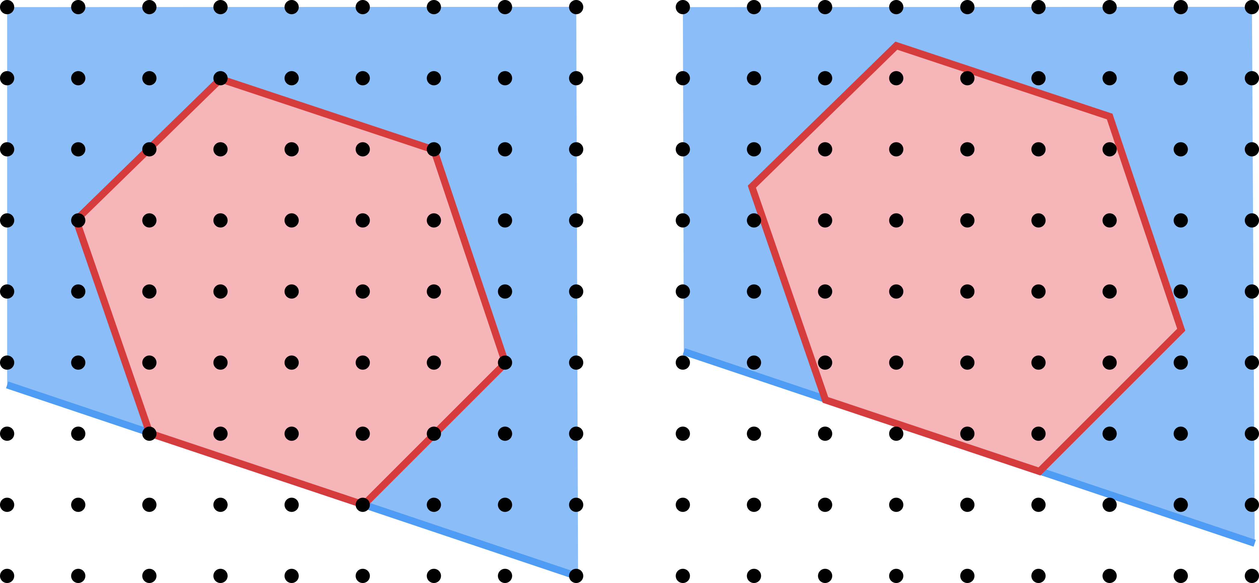
Figure 1: On the left, a lattice polytope with the cone at a 1-dimensional face shaded blue. On the right, the same after a shift by a generic $\lambda$.

3.1.4

Pick an arbitrary vector $\lambda\in\mathfrak{a}^{*}$ and let

$$\Delta_{\lambda}=\Delta+\lambda$$

be the translate of $\Delta$ by the vector $\lambda$. It is a polytope, but no longer with integral vertices.

The same formula (39) defines a sheaf $\mathscr{O}(\Delta_{\lambda})$ on $\overline{\mathsf{A}}$. Note, however, that this sheaf may fail to be locally free if $\overline{\mathsf{A}}$ is singular.

3.1.5

We observe that

$$H^{0}(\overline{\mathsf{A}},\mathscr{O}(\Delta_{\lambda}))=\mathscr{P}_{\Delta_{\lambda},\mathsf{A}}\,,$$ (40)

where for any $\Omega\subset\mathfrak{a}^{*}$ we denote by

$$\mathscr{P}_{\Omega,\mathsf{A}}=\bigoplus_{\mu\in\Omega\cap\operatorname{char}(\mathsf{A})}\mathscr{R}\,a^{\mu}\subset\mathscr{R}[\mathsf{A}]$$

the set of polynomials with Newton polygon inside $\Omega$.

3.1.6

Clearly, there exist a locally finite periodic rational hyperplane arrangement in $\mathfrak{a}^{*}$, such that $\mathscr{O}(\Delta_{\lambda})$ does not change along the strata of this arrangement. Therefore, we may assume, without loss of generality, that

$$\lambda\in\mathfrak{a}_{\mathbb{Q}}^{*}=\operatorname{char}(\mathsf{A})\otimes_{\mathbb{Z}}\mathbb{Q}\,.$$

In this case, the toric variety $\overline{\mathsf{A}}$ and the sheaf $\mathscr{O}(\Delta_{\lambda})$ may be defined in one step by

$$(\overline{\mathsf{A}},\mathscr{O}(\Delta_{\lambda}))=\operatorname{Proj}\bigoplus_{n\geq 0}\mathscr{P}_{n\Delta_{\lambda},\mathsf{A}}\,.$$ (41)

3.1.7

Let $N$ be the order of $\lambda$ in $\mathfrak{a}^{*}_{\mathbb{Q}}/\operatorname{char}(\mathsf{A})$ and consider the torus $\mathsf{A}_{N}$ with character lattice generated by $\lambda$ and $\operatorname{char}(\mathsf{A})$. We have

$$1\to\mu_{N}\to\mathsf{A}_{N}\to\mathsf{A}\to 1\,,$$ (42)

by construction. Consider

$$(\overline{\mathsf{A}}_{N},\mathscr{O}(\Delta_{\lambda})) =\operatorname{Proj}\bigoplus_{n\geq 0}\mathscr{P}_{n\Delta_{\lambda},\mathsf{A}_{N}}$$

$$\cong(\overline{\mathsf{A}}_{N},\mathscr{O}(\Delta)\,a^{\lambda})\,,$$ (43)

where $a^{\lambda}$ is a character of $\mathsf{A}_{N}$. The following is immediate

Lemma 3.1.

We have

$$(\overline{\mathsf{A}},\mathscr{O}(\Delta_{\lambda}))=(\overline{\mathsf{A}}_{N},\mathscr{O}(\Delta)\,a^{\lambda})\Big{/}\!\!\!\!\Big{/}\mu_{N}\,.$$ (44)

3.1.8

We abbreviate

$$\mathscr{O}(\Delta_{\lambda}-\Delta)=\mathscr{O}(\Delta_{\lambda})\otimes\mathscr{O}(\Delta)^{-1}\,.$$

The toric analog of (28) that we will need is the following

Proposition 3.2.

$$H^{i}(\overline{\mathsf{A}},\mathscr{O}(\Delta_{\lambda}-\Delta))=\begin{cases}\mathscr{R}\,a^{\lambda}\,,&i=0\,,\lambda\in\operatorname{char}(\mathsf{A})\,,\\ 0\,,&\textup{otherwise}\,.\end{cases}$$ (45)

Proof.

On $\overline{\mathsf{A}}_{N}$ we have

$$\mathscr{O}_{\overline{\mathsf{A}}_{N}}(\Delta_{\lambda}-\Delta)=\mathscr{O}_{\overline{\mathsf{A}}_{N}}\,a^{\lambda}\,,$$

and therefore

$$H^{i}(\overline{\mathsf{A}}_{N},\mathscr{O}(\Delta_{\lambda}-\Delta))=\begin{cases}\mathscr{R}\,a^{\lambda}\,,&i=0\\ 0\,,&i>0\,.\end{cases}$$ (46)

Taking $\mu_{N}$-invariants concludes the proof. ∎

3.1.9

Let

$$P(a)\in H^{0}(\mathsf{A},\mathscr{O}(\Delta))$$

be a polynomial with Newton polygon $\Delta$. We will call it nondegenerate if the coefficients of $P$ corresponding to the vertices of $\Delta$ are units in $\mathscr{R}$.

Consider the reduction modulo $P$ map

$$H^{0}(\mathsf{A},\mathscr{O}(\Delta_{\lambda}))\to H^{0}(\mathsf{A},\mathscr{O}(\Delta_{\lambda})\big{|}_{P=0})\,.$$ (47)

The vanishing (45) gives the following interpolation property for polynomials with Newton polygon inside $\Delta_{\lambda}$.

Proposition 3.3.

Assume $P$ is nondegenerate. Then the map (47) is surjective. It is also injective if $\lambda\notin\operatorname{char}(\mathsf{A})$. If $\lambda$ is weight of $\mathsf{A}$, then the kernel of (47) equals $\mathscr{R}a^{\lambda}P(a)$.

Proof.

The nondegeneracy of $P$ implies the sequence

$$0\to\mathscr{O}(-\Delta)\xrightarrow{\,\,P\,\,}\mathscr{O}\to\mathscr{O}/P\to 0$$

of sheaves on $\overline{\mathsf{A}}$ is exact. Tensoring it with $\mathscr{O}(\Delta_{\lambda})$ and taking cohomology proves the proposition. ∎

3.2 Stable envelopes in equivariant K-theory

3.2.1

For simplicity, we assume that $X$ has a polarization $T^{1/2}$ with respect to $\mathsf{A}$. We refer to [Opcmi] for a general discussion of stable envelopes in equivariant K-theory in this context.

In elliptic cohomology, we have the flexibility of twisting the attractive line bundle $\mathscr{S}$ by $\mathscr{U}(L,z)$, where $L$ is a line bundle on $X$. We exploited this flexibility in Proposition 2.6. The corresponding parameter in equivariant K-theory is a fractional line bundle

$$L\in\operatorname{Pic}(X)\otimes_{\mathbb{Z}}\mathbb{R}$$

known as slope.

3.2.2

By definition

$$\mathsf{Stab}\in K_{\mathsf{T}}(X\times X^{\mathsf{A}})$$

is an extension of attracting manifold to a K-theory class supported on $\mathsf{Attr}^{f}$ that satisfies

$$\deg_{\mathsf{A}}\mathsf{Stab}\big{|}_{F_{j}\times F_{i}}\subset\deg_{\mathsf{A}}{\Lambda}^{\!\raisebox{1.42262pt}{$\scriptscriptstyle\bullet$}}\!\left(T^{1/2}\right)^{\vee}\big{|}_{F_{j}}+\operatorname{weight}_{\mathsf{A}}\left(L\big{|}_{F_{j}}\right)-\operatorname{weight}_{\mathsf{A}}\left(L\big{|}_{F_{i}}\right)\,.$$ (48)

Here

$$\deg_{\mathsf{A}}f(a)=\textup{Newton polytope}(f)\subset\mathfrak{a}^{*}$$

is the convex hull of nonzero coefficients of $f$.

3.2.3

For a K-theory class supported on $\mathsf{Attr}^{f}$, the condition (48) is equivalent to the, a priori, stronger condition that

$$\deg_{\mathsf{A}^{\prime}}\mathsf{Stab}\big{|}_{F^{\prime}\times F_{i}}\subset\deg_{\mathsf{A}^{\prime}}{\Lambda}^{\!\raisebox{1.42262pt}{$\scriptscriptstyle\bullet$}}\!\left(T^{1/2}\right)^{\vee}\big{|}_{F^{\prime}}+\operatorname{weight}_{\mathsf{A}^{\prime}}\left(L\big{|}_{F^{\prime}}\right)-\operatorname{weight}_{\mathsf{A}^{\prime}}\left(L\big{|}_{F_{i}}\right)\,.$$ (49)

for any subtorus $\mathsf{A}^{\prime}\subset\mathsf{A}$ and any component $F^{\prime}$ of restriction to $X^{\mathsf{A}^{\prime}}$. The polytopes in (49) are the projections of the corresponding polytopes in (48) to $(\mathfrak{a}^{\prime})^{*}$.

3.2.4

Following the logic of the proof of Theorem 1, we consider the K-theory analog of (36)

$$0\to K_{\mathsf{T}}(\mathsf{Attr}(F_{i})\times F_{0})\to K_{\mathsf{T}}(\mathsf{X}_{<i}\times F_{0})\to K_{\mathsf{T}}(\mathsf{X}_{i}\times F_{0})\to 0\,.$$ (50)

In topological K-theory, we may replace $\mathsf{X}_{<i}$ by

$$\mathsf{X}^{\prime}_{<i} :=\textup{total space of the normal bundle $\mathscr{N}$ to $\mathsf{Attr}(F_{i})$}$$

$$\mathsf{X}^{\prime}_{i} :=\textup{complement of the zero section of $\mathscr{N}$}\,.$$

Then the sequence (50) becomes

$$0\to\mathscr{R}[\mathsf{A}]\xrightarrow{\,\,P\,\,}\mathscr{R}[\mathsf{A}]\to\mathscr{R}[\mathsf{A}]/P\to 0\,,$$ (51)

with

$$\mathscr{R}=K_{\mathsf{T}/\mathsf{A}}(F_{i}\times F_{0})$$

and

$$P=\sum(-1)^{k}\Lambda^{k}\mathscr{N}^{\vee}\,.$$ (52)

3.2.5

Lemma 3.4.

The polynomial (52) is nondegenerate in the sense of Section 3.1.9.

Proof.

Let $\eta\in\mathfrak{a}^{*}$ be a vertex of the Newton polytope of $P$. Since it is a vertex, there exists $\xi\in\mathfrak{a}$ such that $\eta$ is the unique maximum of $\xi$ on the polytope.

Decompose $\mathscr{N}$ according to the characters of $\mathsf{A}$

$$\mathscr{N}=\bigoplus a^{\mu}\,\mathscr{N}_{\mu}\,,$$ (53)

and note that

$$\langle\mu,\xi\rangle\neq 0$$

if $\xi$ is chosen generically. Then

$$P=\pm\Lambda^{\textup{top}}\left(\bigoplus_{\langle\mu,\xi\rangle<0}\mathscr{N}^{\vee}_{\mu}\right)\,a^{\eta}+\dots$$

where dots stand for terms of lower weight with respect to $\xi$. ∎

3.2.6

From (53) we conclude

$$P(a)=\prod_{\textup{indivisible $\nu$}}P_{\nu}(a^{\nu})\,.$$

This corresponds to the decomposition

$$\operatorname{Spec}K_{\mathsf{T}}(\mathsf{X}^{\prime}_{i}\times F_{0}) =\operatorname{Spec}\mathscr{R}[\mathsf{A}]/P$$

$$=\bigcup_{\textup{indivisible $\nu$}}\operatorname{Spec}\mathscr{R}[\mathsf{A}]/P_{\nu}$$

$$=\bigcup_{\operatorname{codim}\mathsf{A}^{\prime}=1}\operatorname{Spec}K_{\mathsf{T}}((\mathsf{X}^{\prime}_{i})^{\mathsf{A}^{\prime}}\times F_{0})$$ (54)

where the bijection between indivisible characters $\nu$ and codimension one subtori $\mathsf{A}^{\prime}\subset\mathsf{A}$ is given by

$$1\to\mathsf{A}^{\prime}\to\mathsf{A}\xrightarrow{a^{\nu}}\mathbb{C}^{\times}\to 1\,.$$

3.2.7

We now apply Proposition 3.3 with

$$\Delta =\deg_{\mathsf{A}}{\Lambda}^{\!\raisebox{1.42262pt}{$\scriptscriptstyle\bullet$}}\!\left(T^{1/2}\right)^{\vee}\big{|}_{F_{i}}\,,$$

$$\lambda =\operatorname{weight}_{\mathsf{A}}\left(L\big{|}_{F_{i}}\right)-\operatorname{weight}_{\mathsf{A}}\left(L\big{|}_{F_{0}}\right)\,.$$

By (49), (54) and the inductive hypothesis, $\mathsf{Stab}\big{|}_{\mathsf{X}^{\prime}_{i}\times F_{0}}$ gives an element of $H^{0}(\overline{\mathsf{A}},\mathscr{O}(\Delta_{\lambda})\big{|}_{P=0})$, which can be lifted to an element of $H^{0}(\overline{\mathsf{A}},\mathscr{O}(\Delta_{\lambda}))$. This lift is unique if $\lambda$ is not integral. This gives a proof of the following

Theorem 2.

Stable envelopes exist in equivariant topological K-theory. Further, they are unique if

$$\operatorname{weight}_{\mathsf{A}}\left(L\big{|}_{F_{j}}\right)-\operatorname{weight}_{\mathsf{A}}\left(L\big{|}_{F_{i}}\right)\notin\operatorname{char}(\mathsf{A})$$

for every pair $F_{j}<F_{i}$.

3.2.8

The above argument may be also adapted to work in algebraic K-theory, e.g. by first constructing stable envelopes for a generic attracting cocharacter $\sigma:\mathbb{C}^{\times}\to\mathsf{A}$ and then checking the condition (49) inductively on formal neighborhoods. However, a much stronger result in $D^{b}\operatorname{Coh}X$ has been already established in [16] and we refer the reader there for details.

3.3 Compactified K-theory

The logic of Section 3.2 suggests the following partial compactification of $\operatorname{Spec}K_{\mathsf{T}}(\mathsf{X})$.

3.3.1

Consider the fan in $\mathfrak{a}$ defined in Section 1.3.2 and call it the inertia fan of $\mathsf{X}$. Recall that we have fixed a cone $\mathfrak{C}$ of maximal dimension in this fan. This choice will not play a role in the current discussion. Let $\mathfrak{C}^{\prime}$ be a cone of some dimension in the inertia fan. It defines a subtorus $\mathsf{A}^{\prime}\subset\mathsf{A}$, with

$$\mathfrak{a}^{\prime}=\operatorname{Lie}_{\mathbb{R}}\mathsf{A}^{\prime}=\operatorname{span}(\mathfrak{C}^{\prime})$$

and a choice of attracting/repelling directions for the $\mathsf{A}$-action on $\mathsf{X}^{\mathsf{A}^{\prime}}$.

One should think of each linear subspace $\mathfrak{a}^{\prime}$ as being decorated by the fixed locus $\mathsf{X}^{\mathsf{A}^{\prime}}$ together with the weights of its normal bundle. Those are the weights $\{w_{i}\}$ of Section 1.3.2 that do not vanish on $\mathfrak{a}^{\prime}$. The fan itself records the weights $\{w_{i}\}$ only up to proportionality and without multiplicity.

3.3.2

This fan gives a toric compactification $\overline{\mathsf{A}}$ of $\mathsf{A}$, and thus a partial toric compactification of $\overline{\mathsf{T}}\supset\mathsf{T}$. Boundary strata correspond to cones $\mathfrak{C}^{\prime}$. As we approach a boundary stratum , we go to a particular infinity $0_{\mathfrak{C}^{\prime}}$ in the torus $\mathsf{A}^{\prime}$. The coordinates in $\mathsf{T}/\mathsf{A}^{\prime}$ are the coordinates on the boundary stratum.

For any splitting of

$$1\to\mathsf{A}^{\prime}\to\mathsf{T}\to\mathsf{T}/\mathsf{A}^{\prime}\to 1\,,$$ (55)

we have

(56)

With our hypotheses, the family (56) extends over a neighborhood of $0_{\mathfrak{C}^{\prime}}$. This is independent of the choice of the splitting and gives a partial compactification $\overline{K}_{\mathsf{T}}(\mathsf{X})$ of $\operatorname{Spec}K_{\mathsf{T}}(\mathsf{X})$ over $\overline{\mathsf{T}}$ such that

(57)

where $\mathsf{T}/\mathsf{A}^{\prime}$ is embedded as a boundary stratum. Note that $K_{\mathsf{T}}$ denotes a ring, while $\overline{K}_{\mathsf{T}}$ denotes a scheme. This makes sense, because $\overline{K}_{\mathsf{T}}$ is not affine.

3.3.3

Recall that a line bundle $\mathscr{L}$ on a toric variety $\overline{\mathsf{T}}$ is specified by a function

$$\operatorname{ord}:\mathfrak{a}\to\mathbb{R}$$ (58)

which is continuous and integral linear on the cones of the fan. The sections $f$ of $\mathscr{L}$ are characterized by

$$f=O(a^{\operatorname{ord}})\,,\quad a\to 0_{\mathfrak{C}^{\prime}}\,,$$

for all cones $\mathfrak{C}^{\prime}$. In what follows, we relax the integrality assumption on the function (58). This allows the sheaves $\mathscr{O}(\Delta_{\lambda})$ considered in Section 3.1.4.

To construct a line bundle on $\overline{K}_{\mathsf{T}}(\mathsf{X})$, we may use a different functions (58) on different components $F$ of the fixed locus, as long as these glue over different strata. Given a polarization $T^{1/2}$ and a slope $L$, we define the line bundle $\mathscr{S}(T^{1/2},L)$ by

$$\operatorname{ord}_{\mathscr{S}(T^{1/2},L)}=\textup{maximal weight in }L\otimes\left({\Lambda}^{\!\raisebox{1.42262pt}{$\scriptscriptstyle\bullet$}}\!\,T^{1/2}\right)^{\vee}\,,\quad a\to 0_{\mathfrak{C}^{\prime}}\,.$$

With this definition, the degree bound (49) is equivalent to being a global section of $\mathscr{S}$. Note that the last term in (49) is a constant from our current perspective and may be absorbed into the choice of linearization of $L$.

3.3.4

Note we may replace the polarization $T^{1/2}$ by any other virtual bundle $\mathscr{V}$ on $\mathsf{X}$, as long as the weights of $\mathscr{V}$ define a fan which refines the inertia fan. For instance, one can use the tangent bundle to get a line bundle which is, basically, the square of $\mathscr{S}$.

3.3.5

Recall that, by definition

$$\textup{induced polarization of $\mathsf{X}^{\mathsf{A}^{\prime}}$}=\left(T^{1/2}\big{|}_{\mathsf{X}^{\mathsf{A}^{\prime}}}\right)^{\mathsf{A}^{\prime}}\,.$$ (59)

Similarly, $L\big{|}_{\mathsf{X}^{\mathsf{A}^{\prime}}}$ gives the induced slope.

In the compactification (57), the same fixed locus $\mathsf{X}^{\mathsf{A}^{\prime}}$ appears at several infinities, and the natural polarization of all these copies is different.

Definition 5.

Given $0_{\mathfrak{C}^{\prime}}\in\overline{\mathsf{A}^{\prime}}$ and virtual vector bundle $\mathscr{V}$, we define

$$\mathscr{V}_{\lim}=\mathscr{V}\big{|}_{\mathsf{X}^{\mathsf{A}^{\prime}},\geq 0}-\mathscr{V}^{\vee}\big{|}_{\mathsf{X}^{\mathsf{A}^{\prime}},<0}\,,$$ (60)

where the subscripts refer to nonrepelling and repelling directions as $a\to 0_{\mathfrak{C}^{\prime}}$.

Note that we can write

$$\mathscr{V}_{\lim}=\left(\mathscr{V}\big{|}_{\mathsf{X}^{\mathsf{A}^{\prime}}}\right)^{\mathsf{A}^{\prime}}+\delta\mathscr{V}-\delta\mathscr{V}^{\vee}\,,\quad\delta\mathscr{V}=\mathscr{V}\big{|}_{\mathsf{X}^{\mathsf{A}^{\prime}},>0}\,.$$ (61)

In particular, the limit of a polarization is a polarization. It differs from the induced polarization precisely by the $\delta\mathscr{V}-\delta\mathscr{V}^{\vee}$ term in (61).

We have the following simple

Lemma 3.5.

The boundary strata of $(\overline{K}_{\mathsf{T}}(\mathsf{X}),\mathscr{S})$ have the form $(\overline{K}_{\mathsf{T}}(\mathsf{X}^{\mathsf{A}^{\prime}}),\mathscr{S}_{\lim})$, where $\mathscr{S}_{\lim}$ is defined using the limit polarization and the induced slope.

Proof.

Follows from

$$1-w^{-1}\sim\begin{cases}(1-w^{-1})\big{/}(1-w^{-1})\,,&w\to\infty\,,\\ (1-w^{-1})\big{/}(1-w)\,,&w\to 0\,.\end{cases}$$

∎

3.3.6

Recall that every change in polarization may be compensated by a change in the slope. In particular, we have

$$\deg_{\mathsf{A}}{\Lambda}^{\!\raisebox{1.42262pt}{$\scriptscriptstyle\bullet$}}\!\,\,T^{1/2}_{\lim}=\deg_{\mathsf{A}}\det N^{1/2}_{>0}\otimes{\Lambda}^{\!\raisebox{1.42262pt}{$\scriptscriptstyle\bullet$}}\!\,\,T^{1/2}_{\textup{ind}}\,,$$ (62)

where $N^{1/2}_{>0}$ is the attracting part of the polarization restricted to $\mathsf{X}^{\mathsf{A}^{\prime}}$. Therefore,

$$\mathscr{S}_{\lim}=\mathscr{S}\left(T^{1/2}_{\lim},L_{\textup{ind}}\right)=\mathscr{S}\left(T^{1/2}_{\textup{ind}},L_{\lim}\right)\,,$$

where

$$L_{\lim}=L\otimes(\det N^{1/2}_{>0})^{-1}\,.$$

3.3.7

Recall from formula (9.1.6) in [Opcmi] that stable envelopes may be normalized so that

$$\mathsf{Stab}\big{|}_{\operatorname{diag}\mathsf{X}^{\mathsf{A}}}=(-1)^{-\operatorname{rk}N^{1/2}_{>0}}\left(\frac{\det N_{<0}}{\det N^{1/2}}\right)^{1/2}\,\mathscr{O}_{\mathsf{Attr}}\,,$$ (63)

where $N^{1/2}$ denote the moving part of $T^{1/2}\big{|}_{\mathsf{X}^{\mathsf{A}}}$ and subscripts denote attracting and repelling directions for the chamber $\mathfrak{C}$ as in Section 1.3.2. The following is straightforward:

Lemma 3.6.

The limit of (63) as $a\to 0_{\mathfrak{C}}^{\prime}$ is the same expression for the limit polarization.

3.3.8

Proposition 3.7.

Let $F$ be a component of $\mathsf{X}^{\mathsf{A}}$ and let the slope $L$ be generic and linearized so that it has zero $\mathsf{A}$-weight on $F$. For any $\alpha\in K_{\mathsf{T}/\mathsf{A}}(F)$, we have

$$\mathsf{Stab}_{T^{1/2},L}\,\alpha\in H^{0}\left(\overline{K}_{\mathsf{T}}(\mathsf{X}),\mathscr{S}(T^{1/2},L)\right)$$ (64)

and its restriction to the boundary are the stable envelopes for $\mathsf{X}^{\mathsf{A}^{\prime}}$, extended by zero outside the component containing $F$.

Proof.

Only the statement about restriction to the boundary requires proof. Restriction to the boundary means taking the coefficient of $a^{\operatorname{ord}}$ as $a\to 0_{\mathfrak{C}^{\prime}}$. It can only be nonzero if the function $\operatorname{ord}$ is integral on $\mathfrak{C}^{\prime}$. Therefore, by Lemma 2.7 and genericity of $L$, the restriction to the boundary vanishes outside of the connected component containing $F$.

On the connected component of $\overline{K}_{\mathsf{T}}(\mathsf{X}^{\mathsf{A}^{\prime}})$ containing $F$, the restriction of $\mathsf{Stab}_{T^{1/2},L}\,\alpha$ satisfies the degree bounds for stable envelopes. By Lemma 3.6, it correctly restricts to $F$. Thus it is the stable envelope for the $\mathsf{A}$-action on $\mathsf{X}^{\mathsf{A}^{\prime}}$. ∎

4 Nodal degeneration of stable envelopes

4.1 $\operatorname{Ell}_{\mathsf{T}}(\operatorname{pt})$ near a node

4.1.1

Equivariant cohomology theories over $\mathsf{B}$ are constructed from $1$-dimensional group schemes over $\mathsf{B}$ and, in this section, we are interested in the case when a nodal fiber $E_{0}$ appears in a family of elliptic curves. In a neighborhood of the nodal fiber (formal or analytic), there is a relation between $K_{\mathsf{T}}(\mathsf{X})$ and $\operatorname{Ell}_{\mathsf{T}}(\mathsf{X})$. Our goal is to explain this relation and verify that it respects stable envelopes.

4.1.2

Over a field, the identity component of the group smooth points of $E_{0}$ is a torus of rank 1, which may require a quadratic extension to split. For simplicity, let us assume it is split. Moreover, as our local model, we will take $\mathsf{B}=\operatorname{Spec}\mathscr{R}[[q]]$, where $\mathscr{R}$ is a commutative ring with unit, and

(65)

see Appendix C.1 for a reminder about Tate’s construction of $\mathbb{G}_{\mathbf{m}}/q^{\mathbb{Z}}$.

Tate’s construction only requires the convergence of the standard $\vartheta$-series (105). Therefore, one could replace $\mathscr{R}[[q]]$ with any complete normed commutative ring with a nonzerodivisor $q$ of norm $\|q\|<1$, for instance functions holomorphic in the unit disk of $\mathbb{C}$.

4.1.3

For brevity, we denote $\mathscr{E}=\operatorname{Ell}_{\mathsf{T}}(\operatorname{pt})$. We begin with general remarks about the structure of $\mathscr{O}_{\operatorname{Ell}_{\mathsf{T}}(\mathsf{X})}$ as a sheaf over $\mathscr{E}$. We observe that it belongs to a certain abelian subcategory of $\operatorname{Coh}\mathscr{E}$, which is independent of $q$.

4.1.4

The manifold $\mathsf{X}$ may be represented by a cell complex built from $\mathsf{T}$-equivariant cells of the form $\mathsf{T}/\Gamma\times D^{n}$, where $\Gamma\subset\mathsf{T}$ is a subgroup and $\mathsf{T}$ acts trivially on the disc $D^{n}$. Note that only finitely many possible stabilizers $\Gamma$ appear for a given $\mathsf{X}$. We call them the inertia subgroups of $\mathsf{X}$ and denote their set by $\boldsymbol{\Gamma}_{\mathsf{X}}=\{\Gamma\}$. The sets

$$\{\log\Gamma\}_{\Gamma\in\boldsymbol{\Gamma}_{\mathsf{X}}}\subset\mathfrak{t}=\operatorname{Lie}_{\mathbb{R}}\mathsf{T}\,,$$ (66)

where $\log\Gamma$ is defined in Section C.2.3, form a periodic stratification of $\mathfrak{t}$.

If $\mathsf{X}$ is a smooth manifold, the stratification (66) corresponds to a periodic hyperplane arrangement — the $\mathsf{T}$-weights in the normal bundle to the fixed locus. In general (e.g. by an equivariant embedding into a smooth manifold) we may enlarge the set $\boldsymbol{\Gamma}_{\mathsf{X}}$ so that it corresponds to a periodic hyperplane arrangement. We will assume that this is the case and will refer to (66) as the periodic inertia fan of $\mathsf{X}$, compare with Sections 1.3.2 and 3.3.1.

4.1.5

Reflecting the structure of cell and of the attaching maps, the sheaf $\mathscr{O}_{\operatorname{Ell}_{\mathsf{T}}(X)}$ is built from the sheaves

$$\mathscr{O}_{\operatorname{Ell}_{\mathsf{T}}(\mathsf{T}/\Gamma)}=\iota_{\Gamma,*}\mathscr{O}_{\operatorname{Ell}_{\Gamma}(\operatorname{pt})}\in\operatorname{Coh}\operatorname{Ell}_{\mathsf{T}}(\operatorname{pt})$$

where

$$\iota_{\Gamma}:(\Gamma,\operatorname{pt})\to(\mathsf{T},\operatorname{pt})$$

is an equivariant map. We will identify $\operatorname{Ell}_{\Gamma}(\operatorname{pt})$ with its image under $\iota_{\Gamma}$.

4.1.6

Let $\boldsymbol{\Gamma}=\{\Gamma\}$ be a lattice of subgroups of $\mathsf{T}$. The corresponding $\operatorname{Ell}_{\Gamma}(\operatorname{pt})$ define a stratification of $\mathscr{E}$. Further, the subvarieties

$$\operatorname{diag}\operatorname{Ell}_{\Gamma}(\operatorname{pt})\subset\mathscr{E}^{k}$$ (67)

define a stratification of $\mathscr{E}^{k}$, in which the dimension of consecutive strata differ by $k$.

The following definition is inspired by Bezrukavnikov’s definition of perverse coherent sheaves, see [ArinkBezr].

Definition 6.

Let $f:\mathscr{F}_{1}\to\mathscr{F}_{2}$ be a morphism in $\operatorname{Coh}\mathscr{E}$. We say that $f$ is locally constant with respect to $\boldsymbol{\Gamma}$ if it is a restriction to the diagonal in $\mathscr{E}^{k}$ of a morphism of constant rank along the stratification (67) for $k=2$. We denote the category of locally constant sheaves and locally constant morphism by $\operatorname{Coh}_{\boldsymbol{\Gamma}}\mathscr{E}$.

Proposition 4.1.

For any $\mathsf{T}$-equivariant map $f:X\to Y$ between finite cell complexes, the corresponding map

$$\operatorname{Ell}(f):\mathscr{O}_{\operatorname{Ell}_{\mathsf{T}}(X)}\to\mathscr{O}_{\operatorname{Ell}_{\mathsf{T}}(Y)}$$

is locally constant with respect to the stratification generated by $\boldsymbol{\Gamma}_{X}$ an $\boldsymbol{\Gamma}_{Y}$.

Proof.

Define

$$X^{(2)}=X\times_{X/\mathsf{T}}X\,,$$

where the product is over the quotient by $\mathsf{T}$. This is built from the cells of the form $(\mathsf{T}/\Gamma)^{2}\times D^{n}$, with the attachment maps as before. It has a natural $\mathsf{T}^{2}$ action such that

$$(\mathsf{T},X)\xrightarrow{\quad\operatorname{diag}\quad}(\mathsf{T}^{2},X^{(2)})$$ (68)

is an equivariant morphism. The stabilizers of points now have the form $\operatorname{diag}\Gamma\subset\mathsf{T}^{2}$.

The map $f$ as above gives rise to a $\mathsf{T}^{2}$-equivariant map

$$f^{(2)}:X^{(2)}\to Y^{(2)}$$

and is obtained from it after the restriction to the diagonal (68), which proves the proposition. ∎

Intuitively, the proposition is clear, as the behavior of $f$ on different strata is determined by the corresponding map between fixed points. There are other ways to prove the proposition, for instance, the restriction of $f$ to a any cyclic subgroup of $\mathscr{E}$ should be equivariant with respect to all automorphisms of that subgroup.

4.1.7

The equations of $\Gamma\subset\mathsf{T}$ and $\operatorname{Ell}_{\Gamma}(\operatorname{pt})\subset\operatorname{Ell}_{\mathsf{T}}(\operatorname{pt})$ are encoded by the kernel in the following exact sequence

$$0\to\Gamma^{\perp}\to\operatorname{char}(\mathsf{T})\to\operatorname{char}(\Gamma)\to 0\,.$$

In particular, the divisibility of the generators of $\Gamma^{\perp}$ determines the numbers $\{m_{i}\}$ in

$$\operatorname{Ell}_{\Gamma}(\operatorname{pt})\cong E^{\dim\Gamma}\times\prod E[m_{i}]\,,$$ (69)

where $E[m]$ denotes the scheme of points of order $m$ on $E$.

4.1.8

The category $\operatorname{Coh}_{\boldsymbol{\Gamma}}\mathscr{E}$ is determined by the structure of the lattice $\boldsymbol{\Gamma}$ and the structure of subschemes $E[m]\subset E$ of points of order $m$. Since $E$ is a Tate elliptic curve, we have

$$E[m]\cong\mu_{m}\times\mathbb{Z}/m\mathbb{Z}\,.$$

Here $\mu_{m}\subset\mathbb{G}_{\mathbf{m}}$ is the scheme of $m$th roots of unity and $\mathbb{Z}/m\mathbb{Z}$ is a constant group scheme which records the valuation a point of order $m$ as in (108). As a result, the category $\operatorname{Coh}_{\boldsymbol{\Gamma}}\mathscr{E}$ is independent of $q$.

4.1.9

Our next goal is to construct a degeneration of $\operatorname{Ell}_{\mathsf{T}}(\operatorname{pt})$ in which the inertia subgroups $\operatorname{Ell}_{\Gamma}(\operatorname{pt})$ are transverse to the special fiber and have the exact same structure (in particular, intersect each other in the exact same way) in the special and the generic fibers. This will extend the constant family of subcategories $\operatorname{Coh}_{\boldsymbol{\Gamma}}(\mathscr{E})$ to the central fiber.

While this cannot be achieved for all subgroups of $\mathsf{T}$, for any finite set $\boldsymbol{\Gamma}$ such degeneration may be constructed after a base change of the form $q=(q^{1/M})^{M}$ and a birational transformation. An elementary example is plotted in Figure 2.

Figure 2: In the Legendre family of elliptic curves (left), the subscheme $E[2]$ (plotted in blue) is tangent to the nodal fiber (red). After a base change $q=(q^{1/2})^{2}$ we get a surface which looks like the surface of revolution of the special fiber (right). Blowing up the singular point, we get $E[2]$ to intersects the nodal fiber transversally in 4 points, counting the identity point at infinity. The new nodal fiber is a union of two $\mathbb{P}^{1}$ glued at two points.

4.1.10

In general, a suitable degeneration of $\operatorname{Ell}_{\mathsf{T}}(\operatorname{pt})$ can be constructed in one step as follows, see Appendix C.2. The vector space

$$\mathfrak{t}=\operatorname{cochar}(\mathsf{T})\otimes_{\mathbb{Z}}\mathbb{R}$$

will for now play the role of $\mathfrak{a}$ in Appendix C.2.

The construction of $\mathscr{E}_{\mathscr{Q}}$ in Appendix C.2 involves the following choices:

• a hyperplane arrangement $\mu_{i}(x)\in\mathbb{Z}$ in $\mathfrak{t}$, which refines the periodic fan of $\mathsf{X}$,

• a line bundle $\mathscr{Q}$ on the nodal fiber, which gives the pieces of the dual periodic tessellation of $\mathfrak{t}^{*}$ their particular shape and position.

We call this data the periodic fan and periodic tessellation, respectively. The former describes which weights $\mu_{i}$ appear in

$$\mathscr{Q}=\sum m_{i}\,\mathbb{q}(\mu_{i})+\lambda\,,\quad\lambda\in\mathfrak{t}^{*}_{\mathbb{Q}}\,,$$ (70)

while the latter determines the multiplicities $m_{i}$ and the fractional linear shift $\lambda$.

4.1.11

Degenerations of abelian varieties with an ample line bundle is a well developed theory due to V. Alexeev and his predecessors, see [Alex]. For our bookkeeping purposes, we allow the fractional shift $\lambda$ and thus the orbifold line bundles of the kind discussed in Section 3.1.7 and C.3.

4.1.12

The strata $\eta$ of the period fan and the pieces $\eta^{\vee}$ of the periodic tessellation are in a natural bijection. They also correspond to the toric strata $\left\{O_{\eta}\right\}$ of the nodal fiber of $\mathscr{E}_{\mathscr{Q}}$. Those have the form

$$O_{\eta}=\mathsf{T}/\exp(d\eta)\,,$$

where $d\eta\subset\mathfrak{t}$ is the tangent space to $\eta$ and $\exp(d\eta)$ is the corresponding subtorus as in (118). See Appendix C.2.4.

4.1.13

As everywhere else in this paper, our focus will be on a special subtorus $\mathsf{A}\subset\mathsf{T}$. In particular, we will focus on the restriction to $\mathfrak{a}\subset\mathfrak{t}$ of the hyperplane arrangement corresponding to $\boldsymbol{\Gamma}$. In terms of $q\to 0$ limits of $\vartheta$-functions, this means we assume $\boldsymbol{\nu}(t_{i})=0$, that is,

$$\log t_{i}=o(\log q)\,,\quad q\to 0\,,$$

for all characters $t_{i}$ of $\mathsf{T}/\mathsf{A}$.

4.2 Nodal K-theory

4.2.1

Definition 7.

We define the nodal K-theory $K^{\!\tiny\textknit{U}}_{\mathsf{T}}(\operatorname{pt})_{\mathscr{Q}}$ as the central fiber of $\mathscr{E}_{\mathscr{Q}}$.

4.2.2

The stratifications $\{O_{\eta}\}$ and $\{\operatorname{Ell}_{\Gamma}(\operatorname{pt})\}$ are transverse in the sense that the latter intersects the nodal fiber transversely and

$$O_{\Gamma,\eta}\overset{\textup{\tiny def}}{=}\operatorname{Ell}_{\Gamma}(\operatorname{pt})\cap O_{\eta}\cong\begin{cases}\Gamma/\exp(d\eta)\,,&\eta\subset\log\Gamma\,,\\ \varnothing\,,&\textup{otherwise}\,.\end{cases}$$ (71)

4.2.3

By the transversality (71), the construction of $\operatorname{Ell}_{\mathsf{T}}(\mathsf{X})$ canonically extends to the zero fiber, and we get a scheme

$$K^{\!\tiny\textknit{U}}_{\mathsf{T}}(\mathsf{X})_{\mathscr{Q}}\to K^{\!\tiny\textknit{U}}_{\mathsf{T}}(\operatorname{pt})_{\mathscr{Q}}\,.$$

The neighborhood of any stratum $\eta$ in the periodic fan determines a fan in $\mathfrak{t}/d\eta$. This fan refines the inertia fan of

$$\mathsf{X}^{\eta}\overset{\tiny\textup{def}}{=}\mathsf{X}^{\exp(\eta)}\,,$$

and hence we can use it to construct $\overline{K}_{\mathsf{T}/\exp(d\eta)}(\mathsf{X}^{\eta})$. The following is clear.

Proposition 4.2.

For all $\eta$, we have the following pullback diagram

(72)

4.2.4

There is a finer stratification by subschemes of the form

$$K_{\Gamma,\eta,i}\to O_{\Gamma,\eta}\,,\quad K_{\Gamma,\eta,i}=\operatorname{Spec}K_{\Gamma/\exp(d\eta)}(F_{i})\,,$$ (73)

where $F_{i}$ are the connected components of $\mathsf{X}^{\eta}$.

4.2.5 Example

Suppose $\mathsf{T}\cong\mathbb{C}^{\times}$, $\mathscr{R}$ is a field of $\operatorname{char}\neq 2$, and

$$\boldsymbol{\Gamma}=\{1,\mu_{2},\mathsf{T}\}\,,$$

where $\mu_{2}=\{\pm 1\}$ is the group of square roots of unity. We have

$$\log\mu_{2}=\{0,\tfrac{1}{2}\}+\mathbb{Z}\,,$$

and points $\eta\in\log\mu_{2}$ correspond to two kinds of 1-dimensional strata $\eta^{\vee}\subset\mathfrak{t}^{*}$. The intervals between points in $\log\mu_{2}$ correspond to $0$-dimensional strata in $\mathfrak{t}^{*}$. The combinatorics of the different strata is illustrated in Figure 3.

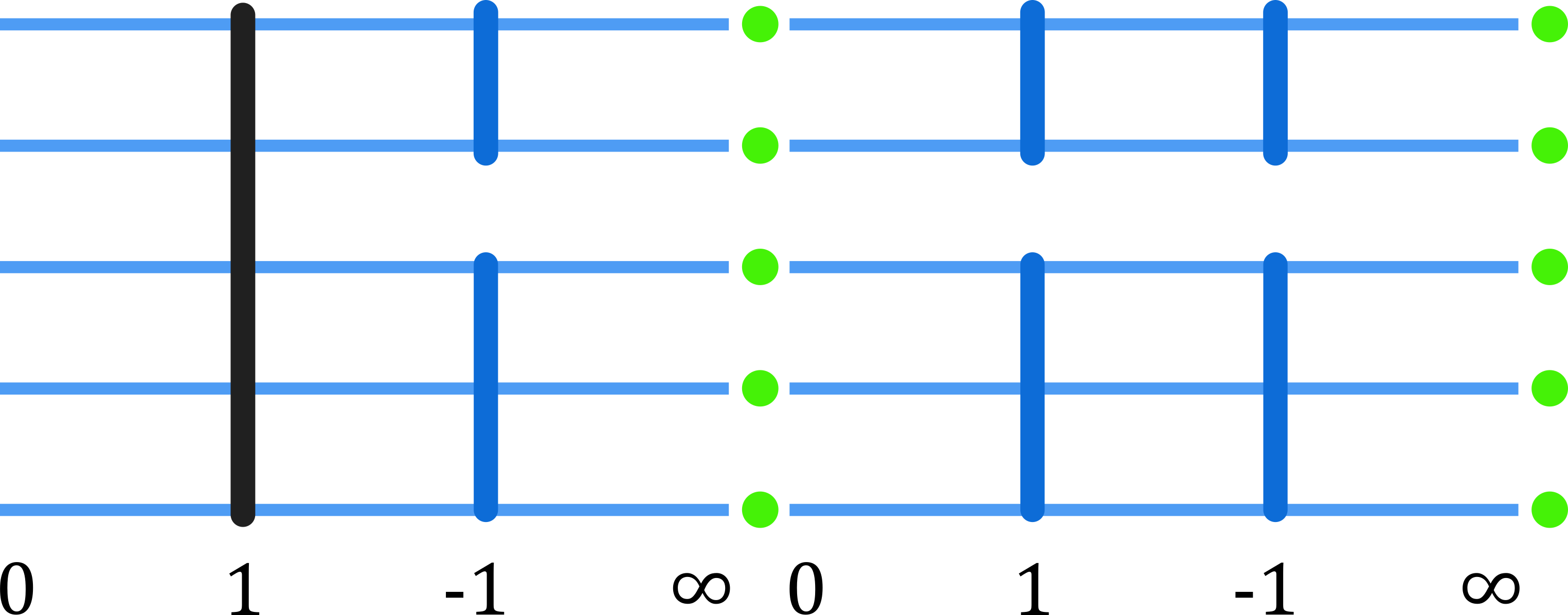
Figure 3: The combinatorics of the strata of $K^{\!\tiny\textknit{U}}_{\mathsf{T}}(\mathsf{X})$, assuming $\mathsf{X}$ is connected, $\mathsf{X}^{\mu_{2}}$ has two components, which break into 2 and 3 components, respectively, in $\mathsf{X}^{\mathsf{T}}$. Strata of the form $K_{\mathsf{T},\eta,i}$ are indicated by connected components; there are three 1-dimensional ones and ten 0-dimensional ones among them. The generic fiber over each $O_{\eta}$ is $\operatorname{Spec}K(\mathsf{X}^{\mathsf{T}})$. We have $K_{1,0}\cong\operatorname{Spec}K(\mathsf{X})$, and the three remaining fibers are isomorphic to $\operatorname{Spec}K(\mathsf{X}^{\mu_{2}})$.

Strata over $O_{0}$ and $O_{\frac{1}{2}}$ have the form $\operatorname{Spec}K_{\mathsf{T}}(\mathsf{X})$ and $\operatorname{Spec}K_{\mathsf{T}}(\mathsf{X}^{\mu_{2}})$, respectively, where the latter is a double cover of $\operatorname{Spec}K_{\mathsf{T}/\mu_{2}}(\mathsf{X}^{\mu_{2}})$. In particular, the fiber $\operatorname{Spec}K(\mathsf{X}^{\mu_{2}})$ appears for a total of three times, corresponding to the nontrivial points of order 2 of $\operatorname{Ell}_{\mathsf{T}}(\operatorname{pt})$.

Also note that, as the picture is trying to suggest, the preimage of the generic point of $O_{\Gamma,\eta}$ need not be dense in $K_{\Gamma,\eta,i}$. For instance, the $\mathsf{T}$ action on $\mathsf{X}$ may be free, in which case $K^{\!\tiny\textknit{U}}_{\mathsf{T}}(\mathsf{X})=K_{1,0}$.

4.2.6

A choice of a component of $X^{\mathsf{T}}$ gives a consistent choice of a component of $X^{\eta}$ for every $\eta$. The corresponding reduced subschemes of $K^{\!\tiny\textknit{U}}_{\mathsf{T}}(X)_{\mathscr{Q}}$ assemble into a copy of $K^{\!\tiny\textknit{U}}_{\mathsf{T}}(\operatorname{pt})_{\mathscr{Q}}$.

In a superficial parallel with the theory of buildings, these reduced subscheme perhaps may be called the floors of $K^{\!\tiny\textknit{U}}_{\mathsf{T}}(X)$. The subsets (72) of maximal dimension, which extend over several floors and share walls with their neighbors, may probably be called the units of $K^{\!\tiny\textknit{U}}_{\mathsf{T}}(X)$. If nodal K-theory proves to be a useful notion, people may find it convenient to refer to different parts of $K^{\!\tiny\textknit{U}}_{\mathsf{T}}(X)$ as slabs, beams, stairwells etc. A floor plan of a real $K^{\!\tiny\textknit{U}}_{\mathsf{T}}(X)$ may be seen in Figure 4.

4.2.7

Conversely, given

$$\mathscr{O}_{K^{\!\tiny\textknit{U}}_{\mathsf{T}}(X)_{\mathscr{Q}}}\in\operatorname{Coh}_{\boldsymbol{\Gamma}}K^{\!\tiny\textknit{U}}_{\mathsf{T}}(\operatorname{pt})_{\mathscr{Q}}$$

it extends canonically in a constant way discussed above to $\mathscr{O}_{\operatorname{Ell}_{\mathsf{T}}(X)}\in\operatorname{Coh}_{\boldsymbol{\Gamma}}\mathscr{E}$ for a Tate elliptic curve. This is, effectively, Grojanowski’s original construction of the equivariant elliptic cohomology over $\mathbb{C}$ in a Tate curve context.

4.3 Theta bundles and stable envelopes

4.3.1

As defined in Section 4.2.3, the scheme $K^{\!\tiny\textknit{U}}_{\mathsf{T}}(\mathsf{X})_{\mathscr{Q}}$ has a stratification and a line bundle inherited from $K^{\!\tiny\textknit{U}}_{\mathsf{T}}(\operatorname{pt})_{\mathscr{Q}}$. This construction may be generalized as in the construction of compactified K-theory, see in particular Section 3.3.4.

Let $\mathscr{V}\in K_{\mathsf{T}}(X)$ be a virtual vector bundle on $\mathsf{X}$ such that all normal weights to $\mathsf{X}^{\mathsf{T}}$ appear as weights of $\mathscr{V}\big{|}_{\mathsf{X}^{\mathsf{T}}}$. For instance, one can take $\mathscr{V}=T\mathsf{X}$. If we only compactify directions in $\mathsf{A}$, we may take

$$\mathscr{V}=T^{1/2}\,.$$

We consider the periodic fan in $\mathfrak{t}$ defined by the weights of $\mathscr{V}\big{|}_{\mathsf{X}^{\mathsf{T}}}$.

4.3.2

For every stratum $\eta$ in the periodic fan, set

$$\mathscr{V}^{\eta}=\left(\mathscr{V}\big{|}_{\mathsf{X}^{\eta}}\right)^{\eta}$$

Let $\eta\to\eta^{\prime}$ indicate that $\eta$ is in the closure of $\eta^{\prime}$. Note the reversal of the arrow, which reflects the fact that $O_{\eta^{\prime}}$ is in the closure of $O_{\eta}$. As in Lemma 3.5, we have

$$\lim_{\eta\to\eta^{\prime}}{\Lambda}^{\!\raisebox{1.42262pt}{$\scriptscriptstyle\bullet$}}\!\,\,\mathscr{V}^{\eta}=\pm\det\delta_{\eta,\eta^{\prime}}\mathscr{V}\otimes{\Lambda}^{\!\raisebox{1.42262pt}{$\scriptscriptstyle\bullet$}}\!\,\,\mathscr{V}^{\eta^{\prime}}\,,\quad\delta_{\eta,\eta^{\prime}}\mathscr{V}=\mathscr{V}^{\eta}\big{|}_{\mathsf{X}^{\eta^{\prime}},>0}\,.$$

Lemma 4.3.

There is a unique, up to multiple, assignment of a line bundle $\boldsymbol{\lambda}_{\eta}\in\operatorname{Pic}_{\mathsf{T}}(\mathsf{X})$ to each stratum $\eta$ such that

$$\det\delta_{\eta,\eta^{\prime}}=\boldsymbol{\lambda}_{\eta}\otimes\boldsymbol{\lambda}_{\eta^{\prime}}^{-1}\,.$$ (74)

Proof.

We need to show that $\delta_{\eta,\eta^{\prime}}$ is a trivial 1-cocycle on the adjacency graph of the strata $\eta$. Loops in this graph are generated by triangles of the form $\eta\to\eta^{\prime}\to\eta^{\prime\prime}$. Since

$$\lim_{\eta\to\eta^{\prime\prime}}=\lim_{\eta^{\prime}\to\eta^{\prime\prime}}\circ\lim_{\eta\to\eta^{\prime}}$$

we have

$$\det\delta_{\eta,\eta^{\prime\prime}}=\det\delta_{\eta,\eta^{\prime}}\otimes\det\delta_{\eta^{\prime},\eta^{\prime\prime}}$$

thus showing the triviality of the cocycle. ∎

We will normalize the choice of $\boldsymbol{\lambda}$ so that $\boldsymbol{\lambda}_{0}$ is trivial.

4.3.3

Definition 8.

We define the nodal K-theory of $\mathsf{X}$ as the union

$$K^{\!\tiny\textknit{U}}_{\mathsf{T}}(\mathsf{T})_{\mathscr{V}}=\bigcup_{\eta}\overline{K}(\mathsf{X}^{\eta})_{\mathscr{V}^{\eta},\boldsymbol{\lambda}_{\eta}}\,.$$ (75)

Given a a fractional line bundle $L\in\operatorname{Pic}_{\mathsf{T}}(X)\otimes\mathbb{Q}$, we denote by $\Theta^{\!\tiny\textknit{U}}(\mathscr{V},L)$ the orbifold line bundle on (75) obtained by gluing $\mathscr{S}(\mathscr{V}^{\eta},L\otimes\boldsymbol{\lambda}_{\eta})$.

Note that for every pair $\eta\to\eta^{\prime}$ there is an inclusion among the corresponding terms in (75). Thus (75) is effectively a union over $0$-dimensional strata $\eta$.

4.3.4 Example

Take $\mathsf{X}=\mathbb{P}^{2}$ and $\mathscr{V}=T\mathsf{X}$, with the action of

$$\mathsf{T}=\operatorname{diag}(a_{1},a_{2},a_{3})\subset PGL(3)\,.$$

Its weights at fixed points are cyclic permutations of $\{a_{2}/a_{1},a_{3}/a_{1}\}$, and the corresponding tiling of each floor is by parallelograms with these sides (often called lozenges), see Figure 4.

Since $\{a_{2}/a_{1},a_{3}/a_{1}\}$ is a basis of $\operatorname{char}(\mathsf{T})$, each lozenge corresponds to a copy of $\mathbb{P}^{1}\times\mathbb{P}^{1}$ in $K^{\!\tiny\textknit{U}}_{\mathsf{T}}(\mathsf{X})$ with a line bundle that is isomorphic to $\mathscr{O}_{\mathbb{P}^{1}}(1)\boxtimes\mathscr{O}_{\mathbb{P}^{1}}(1)$.

The inertia lattice $\boldsymbol{\Gamma}$ has the form

$$\boldsymbol{\Gamma}=\left\{\raisebox{42.67912pt}{\lx@xy@svg{\hbox{\raise 0.0pt\hbox{\kern 21.36366pt\hbox{\ignorespaces\ignorespaces\ignorespaces\hbox{\vtop{\kern 0.0pt\offinterlineskip\halign{\entry@#!@&&\entry@@#!@\cr&\\&&\\&\crcr}}}\ignorespaces{\hbox{\kern-3.0pt\raise 0.0pt\hbox{\hbox{\kern 0.0pt\raise 0.0pt\hbox{\hbox{\kern 3.0pt\raise 0.0pt\hbox{$\textstyle{}$}}}}}}}{\hbox{\kern 60.11621pt\raise 0.0pt\hbox{\hbox{\kern 0.0pt\raise 0.0pt\hbox{\hbox{\kern 3.0pt\raise 0.0pt\hbox{$\textstyle{\mathsf{T}}$}}}}}}}{\hbox{\kern-21.36366pt\raise-38.41666pt\hbox{\hbox{\kern 0.0pt\raise 0.0pt\hbox{\hbox{\kern 3.0pt\raise 0.0pt\hbox{$\textstyle{\{a_{1}=a_{2}\}\ignorespaces\ignorespaces\ignorespaces\ignorespaces}$}}}}}}}\ignorespaces\ignorespaces\ignorespaces{}\ignorespaces\ignorespaces{\hbox{\lx@xy@drawline@}}\ignorespaces{\hbox{\kern 61.51541pt\raise-3.0pt\hbox{\hbox{\kern 0.0pt\raise 0.0pt\hbox{\lx@xy@tip{1}\lx@xy@tip{-1}}}}}}\ignorespaces\ignorespaces{\hbox{\lx@xy@drawline@}}\ignorespaces{\hbox{\lx@xy@drawline@}}{\hbox{\kern 45.36366pt\raise-38.41666pt\hbox{\hbox{\kern 0.0pt\raise 0.0pt\hbox{\hbox{\kern 3.0pt\raise 0.0pt\hbox{$\textstyle{\{a_{1}=a_{3}\}\ignorespaces\ignorespaces\ignorespaces\ignorespaces}$}}}}}}}\ignorespaces\ignorespaces\ignorespaces\ignorespaces{}{\hbox{\lx@xy@droprule}}\ignorespaces{\hbox{\kern 66.72733pt\raise-3.0pt\hbox{\hbox{\kern 0.0pt\raise 0.0pt\hbox{\lx@xy@tip{1}\lx@xy@tip{-1}}}}}}{\hbox{\lx@xy@droprule}}{\hbox{\lx@xy@droprule}}{\hbox{\kern 112.09099pt\raise-38.41666pt\hbox{\hbox{\kern 0.0pt\raise 0.0pt\hbox{\hbox{\kern 3.0pt\raise 0.0pt\hbox{$\textstyle{\{a_{2}=a_{3}\}\ignorespaces\ignorespaces\ignorespaces\ignorespaces}$}}}}}}}\ignorespaces\ignorespaces\ignorespaces{}\ignorespaces\ignorespaces{\hbox{\lx@xy@drawline@}}\ignorespaces{\hbox{\kern 71.93631pt\raise-3.0pt\hbox{\hbox{\kern 0.0pt\raise 0.0pt\hbox{\lx@xy@tip{1}\lx@xy@tip{-1}}}}}}\ignorespaces\ignorespaces{\hbox{\lx@xy@drawline@}}\ignorespaces{\hbox{\lx@xy@drawline@}}{\hbox{\kern-3.0pt\raise-78.41666pt\hbox{\hbox{\kern 0.0pt\raise 0.0pt\hbox{\hbox{\kern 3.0pt\raise 0.0pt\hbox{$\textstyle{}$}}}}}}}{\hbox{\kern 56.22731pt\raise-78.41666pt\hbox{\hbox{\kern 0.0pt\raise 0.0pt\hbox{\hbox{\kern 3.0pt\raise 0.0pt\hbox{$\textstyle{\{1\}\ignorespaces\ignorespaces\ignorespaces\ignorespaces\ignorespaces\ignorespaces\ignorespaces\ignorespaces\ignorespaces\ignorespaces\ignorespaces\ignorespaces}$}}}}}}}\ignorespaces\ignorespaces\ignorespaces{}\ignorespaces\ignorespaces{\hbox{\lx@xy@drawline@}}\ignorespaces{\hbox{\kern 9.16846pt\raise-43.91666pt\hbox{\hbox{\kern 0.0pt\raise 0.0pt\hbox{\lx@xy@tip{1}\lx@xy@tip{-1}}}}}}\ignorespaces\ignorespaces{\hbox{\lx@xy@drawline@}}\ignorespaces{\hbox{\lx@xy@drawline@}}\ignorespaces\ignorespaces\ignorespaces\ignorespaces{}{\hbox{\lx@xy@droprule}}\ignorespaces{\hbox{\kern 66.72733pt\raise-43.91666pt\hbox{\hbox{\kern 0.0pt\raise 0.0pt\hbox{\lx@xy@tip{1}\lx@xy@tip{-1}}}}}}{\hbox{\lx@xy@droprule}}{\hbox{\lx@xy@droprule}}\ignorespaces\ignorespaces\ignorespaces{}\ignorespaces\ignorespaces{\hbox{\lx@xy@drawline@}}\ignorespaces{\hbox{\kern 124.28082pt\raise-43.91666pt\hbox{\hbox{\kern 0.0pt\raise 0.0pt\hbox{\lx@xy@tip{1}\lx@xy@tip{-1}}}}}}\ignorespaces\ignorespaces{\hbox{\lx@xy@drawline@}}\ignorespaces{\hbox{\lx@xy@drawline@}}\ignorespaces}}}}\ignorespaces}\right\}\,. \textstyle{\mathsf{T}} \textstyle{\{a_{1}=a_{2}\}\ignorespaces\ignorespaces\ignorespaces\ignorespaces} \textstyle{\{a_{1}=a_{3}\}\ignorespaces\ignorespaces\ignorespaces\ignorespaces} \textstyle{\{a_{2}=a_{3}\}\ignorespaces\ignorespaces\ignorespaces\ignorespaces} \textstyle{\{1\}\ignorespaces\ignorespaces\ignorespaces\ignorespaces\ignorespaces\ignorespaces\ignorespaces\ignorespaces\ignorespaces\ignorespaces\ignorespaces\ignorespaces} \textstyle{\mathsf{T}} \textstyle{\{a_{1}=a_{2}\}\ignorespaces\ignorespaces\ignorespaces\ignorespaces} \textstyle{\{a_{1}=a_{3}\}\ignorespaces\ignorespaces\ignorespaces\ignorespaces} \textstyle{\{a_{2}=a_{3}\}\ignorespaces\ignorespaces\ignorespaces\ignorespaces} \textstyle{\{1\}\ignorespaces\ignorespaces\ignorespaces\ignorespaces\ignorespaces\ignorespaces\ignorespaces\ignorespaces\ignorespaces\ignorespaces\ignorespaces\ignorespaces}$$

The stratum corresponding to the trivial subgroup $\{1\}$ is at the center of each lozenge. All three floors are glued together there like the three coordinate 2-planes in 3-space. Two floors are glued together where $a_{i}=a_{j}$. See Figure 4.

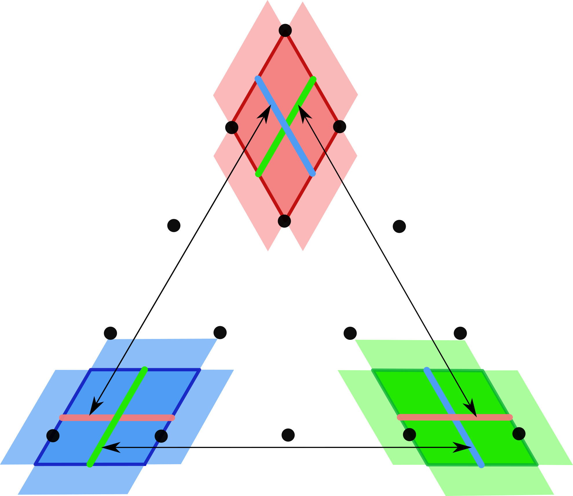
Figure 4: The floors of $K^{\!\tiny\textknit{U}}_{\mathsf{T}}(\mathbb{P}^{2})_{T\mathbb{P}^{2},L}$ plotted with respect to the lattice $\operatorname{char}\mathsf{T}\subset\mathfrak{t}^{*}$. Each floors is tiled by lozenges with sides that are cyclic permutations of $\{a_{2}/a_{1},a_{3}/a_{1}\}$. The tilings are shifted with respect to each other by a weights of a fractional multiple $L$ of $\mathscr{O}_{\mathsf{X}}(1)$, visible as a large triangle (i.e. the toric polytope of $\mathsf{X}$ itself) of fractional size. Arrows indicate gluing. Note that since this picture is in the dual of $\operatorname{Lie}\mathsf{T}$, the gluing is not by embedding, but rather by projection along $\Gamma^{\perp}$.

4.3.5

Proposition 4.4.

The scheme $K^{\!\tiny\textknit{U}}_{\mathsf{T}}(\mathsf{X})_{\mathscr{V}}$ with the line bundle $\Theta^{\!\tiny\textknit{U}}(\mathscr{V},L)$ deforms to $\operatorname{Ell}_{\mathsf{T}}(\mathsf{X})$ with a line bundle which is a Kähler shift of $\Theta(\mathscr{V})$.

Proof.

The cell decomposition of $\mathsf{X}$ exhibits $K^{\!\tiny\textknit{U}}_{\mathsf{T}}(\mathsf{X})_{\mathscr{V}}$ as built out of pieces $K^{\!\tiny\textknit{U}}_{\Gamma}(Y)_{\mathscr{V}}$, where $\Gamma$ acts trivially on $Y$. Thus each of the pieces is a constant thickening of a degeneration of $\operatorname{Ell}_{\Gamma}(\operatorname{pt})$, polarized by a Kähler shift of $\Theta(\mathscr{V})$. Since the deformation is canonical, it is respected by the attachment maps. ∎

4.3.6

Recall from the discussion of compactified K-theory that it is possible to compactify only directions in a subtorus $\mathsf{A}\subset\mathsf{T}$. We can do the same in (75), in which case the periodic fan lies in $\mathfrak{a}$ and we can take $\mathscr{V}=T^{1/2}$.

4.3.7

Theorem 3.

Stable envelopes for $\mathsf{A}$-action on $\mathsf{X}^{\eta}$ glue to a section of $\Theta^{\!\tiny\textknit{U}}(T^{1/2},L)$ and deform to elliptic stable envelopes for $\mathsf{X}$.

Proof.

The first claim follows from Proposition 3.7. Inductive construction of stable envelopes is based on cohomology vanishing, which is semicontinuous. Thus they deform to sections of a Kähler shift of $\Theta(T^{1/2})$. By uniqueness, these sections are elliptic stable envelopes for $\mathsf{X}$. ∎

This results differs by a change of perspective only from an earlier result of Kononov and Smirnov, proven in [17] with somewhat different hypotheses and using different means.

Theorem 4.

[17] The nodal limit of elliptic stable envelopes for $\mathsf{X}$ gives elliptic stable envelopes for $\mathsf{X}^{\Gamma}$, $\Gamma\subset\mathsf{A}$.

Appendix A Constructions in elliptic cohomology

A.1 Chern and Thom classes

A.1.1 Chern classes

A $\mathsf{T}$-equivariant complex vector bundle $V$ of rank $r$ over $\mathsf{X}$ defines a map

$$c:\operatorname{Ell}_{\mathsf{T}}(\mathsf{X})\to\operatorname{Ell}_{GL(r)}(\operatorname{pt})=S^{r}E\,,$$ (76)

see Section (1.8) in [13] and Section 5 in [Ganter]. The coordinates in the target of (76) are symmetric functions on $E^{r}$ — symmetric functions in elliptic Chern roots.

A.1.2 Thom classes

The Thom class of $V$ is, by definition,

$$\Theta(V)=c^{*}\mathscr{O}(D_{\Theta})$$

where $c$ is the map (76) and the divisor

$$D_{\Theta}=\{0\}+S^{r-1}E\subset S^{r}E$$ (77)

is formed by those $r$-tuples that contain $0$.

A.1.3

Note that since $D_{\Theta}$ is effective, we have a canonical section

$$\vartheta_{V}:\mathscr{O}_{\operatorname{Ell}_{\mathsf{T}}\mathsf{X}}\to\Theta(V)\,.$$ (78)

This section may be interpreted as the Euler class of the vector bundle $V$ — the elliptic cohomology class assigned to the locus cut out by a regular section of $V$.

A.1.4

Since

$$\Theta(V_{1}\oplus V_{2})=\Theta(V_{1})\otimes\Theta(V_{2})\,,$$

we have a group homomorphism

$$\Theta:K_{\mathsf{T}}(\mathsf{X})\to\operatorname{Pic}\left(\operatorname{Ell}_{\mathsf{T}}(\mathsf{X})\right)\,.$$ (79)

Also observe that

$$\Theta(V^{\vee})=\Theta(V)$$ (80)

because the divisor (77) is centrally symmetric. The canonical section (78) changes sign by $(-1)^{\operatorname{rk}V}$.

A.1.5

The rank $\operatorname{rk}V$ of a K-theory class on $\mathsf{X}$ is a locally constant function $\mathsf{X}\to\mathbb{Z}$, that is, an element of $H^{0}(\mathsf{X},\mathbb{Z})$. We denote

$$\mathfrak{m}_{1}=\operatorname{Ker}(K_{\mathsf{G}}(\mathsf{X})\xrightarrow{\,\,\operatorname{rk}\,\,}H^{0}(\mathsf{X},\mathbb{Z}))\,.$$

This ideal is the first step in the filtration of $K_{\mathsf{T}}(\mathsf{X})$ by the codimension of support.

Lemma A.1.

The map $V\mapsto\Theta(V)$ factors through the quotient $K_{\mathsf{G}}(\mathsf{X})/\mathfrak{m}_{1}^{3}$.

See Appendix B.1 for the proof.

A.2 Fixed loci

A.2.1

We have two natural maps of the form (7) associated to the fixed locus $\mathsf{X}^{\mathsf{A}}$ namely

$$(\mathsf{T},\mathsf{X}^{\mathsf{A}}) \xrightarrow{\quad\,\,1_{\mathsf{T}}\times\iota\quad\,\,\,\,} \,(\mathsf{T},\mathsf{X})\,,$$ (81)

$$(\mathsf{T},\mathsf{X}^{\mathsf{A}}) \xrightarrow{\quad\phi\times 1_{\mathsf{X}^{\mathsf{A}}}\quad} \,(\mathsf{T}/\mathsf{A},\mathsf{X}^{\mathsf{A}})\,.$$ (82)

where $\iota:\mathsf{X}^{\mathsf{A}}\to\mathsf{X}$ is the inclusion and $\phi:\mathsf{T}\to\mathsf{T}/\mathsf{A}$ is the quotient.

A.2.2

The diagram

$$\lx@xy@svg{\hbox{\raise 0.0pt\hbox{\kern 20.9417pt\hbox{\ignorespaces\ignorespaces\ignorespaces\hbox{\vtop{\kern 0.0pt\offinterlineskip\halign{\entry@#!@&&\entry@@#!@\cr&&\\&&\crcr}}}\ignorespaces{\hbox{\kern-20.9417pt\raise 0.0pt\hbox{\hbox{\kern 0.0pt\raise 0.0pt\hbox{\hbox{\kern 3.0pt\raise 0.0pt\hbox{$\textstyle{\operatorname{Ell}_{\mathsf{T}}(\mathsf{X}^{\mathsf{A}})\ignorespaces\ignorespaces\ignorespaces\ignorespaces\ignorespaces\ignorespaces\ignorespaces\ignorespaces}$}}}}}}}\ignorespaces\ignorespaces\ignorespaces\ignorespaces{}{\hbox{\lx@xy@droprule}}\ignorespaces\ignorespaces\ignorespaces{\hbox{\kern 44.60628pt\raise 6.1111pt\hbox{{}\hbox{\kern 0.0pt\raise 0.0pt\hbox{\hbox{\kern 3.0pt\hbox{\hbox{\kern 0.0pt\raise-1.75pt\hbox{$\scriptstyle{\phi}$}}}\kern 3.0pt}}}}}}\ignorespaces{\hbox{\kern 74.9417pt\raise 0.0pt\hbox{\hbox{\kern 0.0pt\raise 0.0pt\hbox{\lx@xy@tip{1}\lx@xy@tip{-1}}}}}}{\hbox{\lx@xy@droprule}}{\hbox{\lx@xy@droprule}}\ignorespaces\ignorespaces\ignorespaces\ignorespaces{}{\hbox{\lx@xy@droprule}}\ignorespaces\ignorespaces\ignorespaces{\hbox{\kern-9.52188pt\raise-20.64499pt\hbox{{}\hbox{\kern 0.0pt\raise 0.0pt\hbox{\hbox{\kern 3.0pt\hbox{\hbox{\kern 0.0pt\raise-0.8264pt\hbox{$\scriptstyle{p}$}}}\kern 3.0pt}}}}}}\ignorespaces{\hbox{\kern 0.0pt\raise-31.45667pt\hbox{\hbox{\kern 0.0pt\raise 0.0pt\hbox{\lx@xy@tip{1}\lx@xy@tip{-1}}}}}}{\hbox{\lx@xy@droprule}}{\hbox{\lx@xy@droprule}}{\hbox{\kern 44.9417pt\raise 0.0pt\hbox{\hbox{\kern 0.0pt\raise 0.0pt\hbox{\hbox{\kern 3.0pt\raise 0.0pt\hbox{$\textstyle{}$}}}}}}}{\hbox{\kern 74.9417pt\raise 0.0pt\hbox{\hbox{\kern 0.0pt\raise 0.0pt\hbox{\hbox{\kern 3.0pt\raise 0.0pt\hbox{$\textstyle{\operatorname{Ell}_{\mathsf{T}/\mathsf{A}}(\mathsf{X}^{\mathsf{A}})\ignorespaces\ignorespaces\ignorespaces\ignorespaces}$}}}}}}}\ignorespaces\ignorespaces\ignorespaces\ignorespaces{}{\hbox{\lx@xy@droprule}}\ignorespaces\ignorespaces\ignorespaces{\hbox{\kern 99.38339pt\raise-20.64499pt\hbox{{}\hbox{\kern 0.0pt\raise 0.0pt\hbox{\hbox{\kern 3.0pt\hbox{\hbox{\kern 0.0pt\raise-0.8264pt\hbox{$\scriptstyle{p}$}}}\kern 3.0pt}}}}}}\ignorespaces{\hbox{\kern 99.38339pt\raise-31.45667pt\hbox{\hbox{\kern 0.0pt\raise 0.0pt\hbox{\lx@xy@tip{1}\lx@xy@tip{-1}}}}}}{\hbox{\lx@xy@droprule}}{\hbox{\lx@xy@droprule}}{\hbox{\kern-8.425pt\raise-41.28998pt\hbox{\hbox{\kern 0.0pt\raise 0.0pt\hbox{\hbox{\kern 3.0pt\raise 0.0pt\hbox{$\textstyle{\mathscr{E}_{\mathsf{T}}\ignorespaces\ignorespaces\ignorespaces\ignorespaces}$}}}}}}}\ignorespaces\ignorespaces\ignorespaces\ignorespaces{}{\hbox{\lx@xy@droprule}}\ignorespaces\ignorespaces\ignorespaces{\hbox{\kern 44.60628pt\raise-35.17888pt\hbox{{}\hbox{\kern 0.0pt\raise 0.0pt\hbox{\hbox{\kern 3.0pt\hbox{\hbox{\kern 0.0pt\raise-1.75pt\hbox{$\scriptstyle{\phi}$}}}\kern 3.0pt}}}}}}\ignorespaces{\hbox{\kern 87.45839pt\raise-41.28998pt\hbox{\hbox{\kern 0.0pt\raise 0.0pt\hbox{\lx@xy@tip{1}\lx@xy@tip{-1}}}}}}{\hbox{\lx@xy@droprule}}{\hbox{\lx@xy@droprule}}{\hbox{\kern 44.9417pt\raise-41.28998pt\hbox{\hbox{\kern 0.0pt\raise 0.0pt\hbox{\hbox{\kern 3.0pt\raise 0.0pt\hbox{$\textstyle{}$}}}}}}}{\hbox{\kern 87.45839pt\raise-41.28998pt\hbox{\hbox{\kern 0.0pt\raise 0.0pt\hbox{\hbox{\kern 3.0pt\raise 0.0pt\hbox{$\textstyle{\mathscr{E}_{\mathsf{T}/\mathsf{A}}}$}}}}}}}\ignorespaces}}}}\ignorespaces\,, \textstyle{\operatorname{Ell}_{\mathsf{T}}(\mathsf{X}^{\mathsf{A}})\ignorespaces\ignorespaces\ignorespaces\ignorespaces\ignorespaces\ignorespaces\ignorespaces\ignorespaces} \scriptstyle{\phi} \scriptstyle{p} \textstyle{\operatorname{Ell}_{\mathsf{T}/\mathsf{A}}(\mathsf{X}^{\mathsf{A}})\ignorespaces\ignorespaces\ignorespaces\ignorespaces} \scriptstyle{p} \textstyle{\mathscr{E}_{\mathsf{T}}\ignorespaces\ignorespaces\ignorespaces\ignorespaces} \scriptstyle{\phi} \textstyle{\mathscr{E}_{\mathsf{T}/\mathsf{A}}} \textstyle{\operatorname{Ell}_{\mathsf{T}}(\mathsf{X}^{\mathsf{A}})\ignorespaces\ignorespaces\ignorespaces\ignorespaces\ignorespaces\ignorespaces\ignorespaces\ignorespaces} \scriptstyle{\phi} \scriptstyle{p} \textstyle{\operatorname{Ell}_{\mathsf{T}/\mathsf{A}}(\mathsf{X}^{\mathsf{A}})\ignorespaces\ignorespaces\ignorespaces\ignorespaces} \scriptstyle{p} \textstyle{\mathscr{E}_{\mathsf{T}}\ignorespaces\ignorespaces\ignorespaces\ignorespaces} \scriptstyle{\phi} \textstyle{\mathscr{E}_{\mathsf{T}/\mathsf{A}}}$$ (83)

is a pullback diagram. Its horizontal maps are quotients by a free action of $\mathscr{E}_{A}$.

A.2.3

Given a line bundle $\mathscr{L}$ on $\operatorname{Ell}_{\mathsf{T}}(\mathsf{X})$, we denote by $\deg_{\mathsf{A}}$ the degree of its restriction to the fibers of $\phi$ in (83), see Appendix B.3. This degree is an element of $S^{2}\operatorname{char}(\mathsf{A})$ which depends on the component of the fixed locus. In other words:

$$\deg_{\mathsf{A}}:\operatorname{Pic}(\operatorname{Ell}_{\mathsf{T}}(\mathsf{X}))\to H^{0}(X^{\mathsf{A}},S^{2}\operatorname{char}(\mathsf{A}))\,.$$ (84)

For instance,

$$\deg_{\mathsf{A}}\Theta(V)=(c_{1}^{2}-2c_{2})\left(V|_{\operatorname{pt}\in X^{\mathsf{A}}}\right)\,.$$ (85)

where we take equivariant Chern classes of the fiber of $V$ at a point of $X^{\mathsf{A}}$. Formula (85) follows from (101).

A.3 Push-forwards

A.3.1

Recall the functor

$$f_{*}:\operatorname{Coh}\operatorname{Ell}_{\mathsf{G}_{1}}(\mathsf{X}_{1})\to\operatorname{Coh}\operatorname{Ell}_{\mathsf{G}_{2}}(\mathsf{X}_{2})$$ (86)

induced by a map of the form (7).

Pushforwards in equivariant elliptic cohomology are defined for proper complex oriented equivariant maps, and are homomorphisms

$$f_{{\circledast}}\in\operatorname{Hom}_{\operatorname{Coh}\operatorname{Ell}_{\mathsf{G}_{2}}(\mathsf{X}_{2})}(f_{*}\Theta_{\mathsf{X}_{1}}(-N_{f}),\mathscr{O}_{\operatorname{Ell}_{\mathsf{G}_{2}}(\mathsf{X}_{2})})\,,$$ (87)

where $N_{f}\in K_{\mathsf{T}}(\mathsf{X}_{1})$ is the normal bundle to $f$.

A.3.2

Note the difference

$$f_{{\circledast}}\neq f_{*}\,.$$

For starters, $f_{*}$ is a functor, while $f_{{\circledast}}$ is a map in the target category of $f_{*}$.

A.3.3 Duality

Given a line bundle $\mathscr{L}$ on $\operatorname{Ell}_{\mathsf{T}}(\mathsf{X})$, we set

$$\mathscr{L}^{\triangledown}=\mathscr{L}^{-1}\otimes\Theta(T\mathsf{X})\,.$$ (88)

This is the appropriate twist of duality for line bundles in our situation. If $p_{\mathsf{X}}:X\to\operatorname{pt}$ is proper, this gives a pairing

$$p_{\mathsf{X},*}(\mathscr{L}\otimes\mathscr{L}^{\triangledown})\xrightarrow{\quad p_{\mathsf{X},{\circledast}}\quad}\mathscr{O}_{\mathscr{E}_{\mathsf{T}}}\,.$$ (89)

A.3.4 Supports

For any coherent sheaf $\mathscr{G}$ on $\operatorname{Ell}_{\mathsf{T}}(\mathsf{X})$ and any $\mathsf{T}$-invariant open $U\subset\mathsf{X}$, we have a subsheaf

$$\mathscr{G}_{\operatorname{supp}\subset\mathsf{X}\setminus U}=\operatorname{Ker}\left(\mathscr{G}\to\mathscr{G}|_{U}\right)$$ (90)

of sections supported in $\mathsf{X}\setminus U$. The map in (90) is the functorial pullback with respect to the inclusion $U\to\mathsf{X}$.

We will be using (90) for locally free sheaves $\mathscr{G}$.

A.3.5

For general complex oriented maps, we have the following generalization of (91)

$$f_{{\circledast}}\in\operatorname{Hom}_{\operatorname{Coh}\operatorname{Ell}_{\mathsf{G}_{2}}(\mathsf{X}_{2})}(f_{*}\Theta_{\mathsf{X}_{1}}(-N_{f})_{\textup{c}},\mathscr{O}_{\operatorname{Ell}_{\mathsf{G}_{2}}(\mathsf{X}_{2})})\,,$$ (91)

where the subsheaf

$$\Theta_{\mathsf{X}_{1}}(-N_{f})_{\textup{c}}\subset\Theta_{\mathsf{X}_{1}}(-N_{f})$$

is formed by sections $s$ such that $f\big{|}_{\operatorname{supp}s}$ is proper.

A.3.6 Correspondences

Consider the diagram

(92)

in which

$$\mathsf{p}_{1}=1_{\mathsf{X}_{2}}\times p_{1}\,,\quad\mathsf{p}_{2}=p_{2}\times 1_{\mathsf{X}_{1}}\,.$$

In particular

$$N_{\mathsf{p}_{1}}=-\mathsf{p}_{2}^{*}\,T\mathsf{X}_{1}\,.$$

The pull-push formula

$$\alpha\mapsto(\mathsf{p}_{2})_{{\circledast}}(\alpha\mathsf{p}_{1}^{*}(\,\cdot\,))\,,\qquad$$ (93)

gives a map

$$p_{12,*}\Theta_{\mathsf{X}_{1}\times\mathsf{X}_{2}}(\mathsf{p}_{2}^{*}\,T\mathsf{X}_{1})_{\textup{c}}\to\mathscr{H}\!\!\textit{om}\Big{(}p_{1,*}\mathscr{O}_{\operatorname{Ell}_{\mathsf{T}}(\mathsf{X}_{1})},p_{2,*}\mathscr{O}_{\operatorname{Ell}_{\mathsf{T}}(\mathsf{X}_{2})}\Big{)}$$ (94)

of sheaves on $\mathscr{E}_{\mathsf{T}}$. Here

$$p_{12}=p_{1}\circ\mathsf{p}_{2}=p_{2}\circ\mathsf{p}_{1}\,.$$

A.3.7

More generally, if $\mathscr{L}_{i}\in\operatorname{Pic}(\operatorname{Ell}_{\mathsf{T}}(\mathsf{X}_{i}))$ then a section

$$\alpha\in H^{0}(\mathscr{L}_{2}\boxtimes\mathscr{L}_{1}^{\triangledown})$$ (95)

gives a map

$$p_{1,*}\,\mathscr{L}_{1}\xrightarrow{\quad(\mathsf{p}_{1})_{{\circledast}}(\alpha\mathsf{p}_{2}^{*}(\,\cdot\,))\quad}p_{2,*}\,\mathscr{L}_{2}$$ (96)

in $\operatorname{Coh}\mathscr{E}_{\mathsf{T}}$. In (95) and elsewhere, the symbol $\boxtimes$ denotes the tensor product of pullbacks via two projection maps.

A.3.8

Elliptic stable envelopes are objects of the form (95) on $\mathsf{X}\times\mathsf{X}^{\mathsf{A}}$ for certain special lines bundles $\mathscr{L}_{i}$.

A.4 Kähler line bundles

A.4.1

Kähler line bundles give a rich supply of line bundles of $\mathsf{A}$-degree $0$. The terminology is chosen for consistency with [1], because the variables $z$ corresponds to the Kähler parameters in enumerative context.

A.4.2

Let $V$ be vector bundle on $\mathsf{X}$ and let $\mathbb{C}^{\times}_{z}$ be a new copy of the group $\mathbb{C}^{\times}$ with coordinate $z$, acting trivially on $\mathsf{X}$. As in (83), we have

$$\operatorname{Ell}_{\mathsf{T}\times\mathbb{C}^{\times}_{z}}(\mathsf{X})=\operatorname{Ell}_{\mathsf{T}}(\mathsf{X})\times E_{z}\,,\quad E_{z}=\mathscr{E}_{\mathbb{C}^{\times}_{z}}\,.$$ (97)

Consider the K-theory class

$$(z-1)(V-\mathbb{C}^{\operatorname{rk}V})\in\mathfrak{m}_{1}^{2}\subset K_{\mathsf{T}\times\mathbb{C}^{\times}_{z}}(\mathsf{X})\,,$$

where $\mathbb{C}^{\operatorname{rk}V}$ is a trivial bundle of rank $r$. It gives a line bundle

$$\mathscr{U}(V,z)=\Theta((z-1)(V-\mathbb{C}^{\operatorname{rk}V}))\in\operatorname{Pic}(\operatorname{Ell}_{\mathsf{T}}(\mathsf{X})\times E_{z})\,,$$ (98)

which has degree $0$ along each factor.

A.4.3

Clearly,

$$\mathscr{U}(V_{1}\oplus V_{2},z)\cong\mathscr{U}(V_{1},z)\otimes\mathscr{U}(V_{2},z)\,.$$

Lemma A.2.

We have

$$\mathscr{U}(V,z) \cong\mathscr{U}(\det V,z)\,,$$ (99)

$$\mathscr{U}(V,z_{1}z_{2}) \cong\mathscr{U}(V,z_{1})\otimes\mathscr{U}(V,z_{2})\,.$$ (100)

Here $\mathscr{U}(V,z_{1}z_{2})$ is the pullback by the addition map $E\times E\to E$, as in (10).

Proof.

Follows immediately from Lemma A.1  . ∎

A.4.4

By (99) and homotopy invariance, the map $V\mapsto\mathscr{U}(V,z)$ factors through the discrete group

$$K_{\mathsf{T}}(\mathsf{X})\xrightarrow{\quad\det\quad}\operatorname{Pic}_{\mathsf{T}}(\mathsf{X})\xrightarrow{\quad\pi_{0}\quad}NS_{\mathsf{T}}(\mathsf{X})\overset{\tiny\textup{def}}{=}\operatorname{Pic}_{\mathsf{T}}(\mathsf{X})\big{/}\operatorname{Pic}_{\mathsf{T}}(\mathsf{X})_{0}\,.$$

A.4.5

If $V$ pulled back via $f:\mathsf{X}\to Y$, then similarly $\mathscr{U}(V,z)$ is pulled back from $\operatorname{Ell}_{\mathsf{T}}(Y)$. In particular, line bundles $\mathscr{U}(w,z)$, where $w$ is a character of $\mathsf{T}$, are pulled back from $\mathscr{E}_{\mathsf{T}}$.

Appendix B Line bundles on $\mathscr{E}_{\mathsf{A}}$

B.1 Proof of Lemma A.1

Proof.

It suffices to consider the universal case

$$\mathsf{G}=\prod GL(r_{i})\,,\quad\mathsf{X}=\operatorname{pt}\,.$$

To save on notation, we set

$$\mathscr{E}=\operatorname{Ell}_{\mathsf{G}}(\operatorname{pt})=\prod S^{r_{i}}E\,.$$

This is smooth and projective over $\mathsf{B}$.

Consider the diagonal embedding and three projections

$$\mathsf{G}\xrightarrow{\quad\operatorname{diag}\quad}\mathsf{G}^{3}\xrightarrow{\quad p_{1},p_{2},p_{3}\quad}\mathsf{G}\,.$$

The ideal $\mathfrak{m}_{1}^{3}$ is spanned by $V$ of the form

$$V=\operatorname{diag}^{*}\left(p_{1}^{*}(V_{1})\otimes p_{2}^{*}(V_{2})\otimes p_{3}(V_{3})\right)\,,\quad V_{i}\in\mathfrak{m}_{1}\,.$$

Since $V_{i}\in\mathfrak{m}_{1}$, we have $V_{i}\big{|}_{1\in G}=0$. Therefore

$$\left.\Theta\left(\bigotimes p_{i}^{*}(V_{i})\right)\right|_{\{1\}\times\mathscr{E}\times\mathscr{E}}=\mathscr{O}_{\mathscr{E}^{2}}\,,$$

and similarly for the other factors.

By the theorem of the cube, see [28] for a version over a general base scheme $\mathsf{B}$, we have

$$\Theta\left(\bigotimes p_{i}^{*}(V_{i})\right)=\mathscr{O}_{\mathscr{E}^{3}}\,.$$

Therefore $\Theta(V)=\operatorname{diag}^{*}\mathscr{O}_{\mathscr{E}^{3}}=\mathscr{O}_{\mathscr{E}}$, as was to be shown. ∎

B.2 The dual Abelian variety

Since the character lattice $\operatorname{char}(\mathsf{A})$ is dual to the cocharacter lattice in (12) and $E$ is principally polarized, we have

$$\mathscr{E}^{\vee}_{\mathsf{A}}=\operatorname{char}(\mathsf{A})\otimes_{\mathbb{Z}}E=\mathscr{E}_{\mathsf{A}^{\vee}}\,,$$

where $\mathsf{A}^{\vee}$ is the dual torus.

If $\{a_{i}\}$ is a basis of $\operatorname{char}(\mathsf{A})$ and $\{a^{\vee}_{i}\}$ is the dual basis of characters of $\mathsf{A}^{\vee}$ then

$$\eta=\sum(a_{i}-1)(a^{\vee}_{i}-1)\in\mathfrak{m}_{1}^{2}/\mathfrak{m}_{1}^{3}\subset K_{\mathsf{A}\times\mathsf{A}^{\vee}}(\operatorname{pt})/\mathfrak{m}_{1}^{3}$$

is a canonical element and

$$\Theta(\eta)=\textup{Poincar\'{e} line bundle on $\mathscr{E}_{\mathsf{A}}\times\mathscr{E}_{\mathsf{A}^{\vee}}$}\,.$$

B.3 The degree of a line bundle

By definition, we have an exact sequence

$$0\to\operatorname{Pic}_{0}(\mathscr{E})\to\operatorname{Pic}(\mathscr{E})\to\operatorname{NS}(\mathscr{E})\to 0\,,$$

where the discrete group $\operatorname{NS}(\mathscr{E})$ is the Neron-Severi group of $\mathscr{E}$. For an Abelian variety, we have

$$\operatorname{Pic}_{0}(\mathscr{E})=\mathscr{E}^{\vee}\,,\quad\operatorname{NS}(\mathscr{E})=\operatorname{Hom}_{\textup{symmetric}}(\mathscr{E},\mathscr{E}^{\vee})\,.$$

By definition, the degree $\mathscr{L}$ of a line bundle is its class in $\operatorname{NS}(\mathscr{E})$. To compute it, note that $\mathscr{L}$ defines a morphism $\mathscr{E}_{\mathsf{A}}\to\mathscr{E}_{\mathsf{A}^{\vee}}$ by by the formula

$$a\mapsto(\textup{multiplication by $a$})^{*}\mathscr{L}\otimes\mathscr{L}^{-1}\,.$$

We denote this morphism by

$$\deg\mathscr{L}\in\operatorname{Hom}_{\textup{symmetric}}(\mathscr{E}_{\mathsf{A}},\mathscr{E}_{\mathsf{A}}^{\vee})\cong\operatorname{NS}(\mathscr{E})\,.$$

From definitions, if

$$V=\sum_{\mu\in\operatorname{char}(\mathsf{A})}V_{\mu}\,a^{\mu}\in K_{\mathsf{A}}(\mathsf{X}^{\mathsf{A}})$$

then

$$\deg\Theta(V)=\sum\operatorname{rk}(V_{\mu})\,\mu^{2}\in S^{2}\operatorname{char}(\mathsf{A})\subset\operatorname{Hom}_{\textup{symmetric}}(\mathscr{E}_{\mathsf{A}},\mathscr{E}_{\mathsf{A}}^{\vee})\,.$$ (101)

Note that for a very general elliptic curve $E$, we have

$$\operatorname{Hom}(E,E)=\mathbb{Z}\,,$$

and therefore $\operatorname{NS}(\mathscr{E})=S^{2}\operatorname{char}(\mathsf{A})$. We will not encounter line bundles of other degrees in this paper.

Figure 5: The function $\mathbb{q}(x)$

Appendix C Degeneration of Abelian varieties

Degeneration of Abelian varieties is a very rich, old, and well-developed subject, see [Brion] for an introduction to its basics including Alexeev’s theory [Alex]. Here we summarize a few elementary aspects of this theory that will play a role in this paper.

C.1 Tate elliptic curve

Let $\mathbb{q}(x)$ be a solution of

$$\mathbb{q}^{\prime\prime}(x)=\sum_{n\in\mathbb{Z}}\delta(x-n)\,,$$

which vanishes for $x\in[0,1]$. Explicitly,

$$\mathbb{q}(x)=x\lfloor x\rfloor-\tfrac{1}{2}\lfloor x\rfloor(\lfloor x\rfloor+1)$$

see the plot in Figure 5. We note that changing $\mathbb{q}(x)$ by an integral form of degree $\leq 1$ in $x$ does not affect what follows, while the effect of changing it by a rational form of degree $\leq 1$ will be discussed in Section C.3.

Let $\mathscr{R}$ be a ring with unit. The Tate elliptic curve over $\mathscr{R}[[q]]$ is the quotient of the toric surface $\Sigma_{\mathbb{q}}$ over $\mathscr{R}$ with polyhedron

$$\Delta_{\mathbb{q}} =\{(x,y),y\geq\mathbb{q}(x)\}$$

$$=\operatorname{conv}\left\{(k,m)\in\mathbb{Z}^{2},m\geq\frac{1}{2}\,k(k-1)\right\}$$ (102)

by a certain action of $\Lambda\cong\mathbb{Z}$. The completion of $\mathscr{R}[q]$ to $\mathscr{R}[[q]]$ will be required to take the quotient.

By definition,

$$\Sigma_{\mathbb{q}}=\operatorname{Proj}\bigoplus_{\frac{m}{n}\geq\mathbb{q}\left(\frac{k}{n}\right)}\mathscr{R}\,t^{n}a^{k}q^{m}\,,\quad n\geq 0\,,$$ (103)

where the $n=0$ term is interpreted as $\mathscr{R}[q]$ and the grading is by $n$. The fact that the algebra in (103) is not finitely generated should not a be a concern, as the invariants of $\Lambda$ will be finitely generated.

The group $\Lambda$ is generated by the transformation

$$\sigma:(t,a,q)\mapsto(at,qa,q)\,.$$ (104)

In other words,

$$\Lambda=\left\langle{\textstyle\begin{pmatrix}1&0&0\\ 1&1&0\\ 0&1&1\end{pmatrix}}\right\rangle\subset SL(3,\mathbb{Z})\,,$$

acting on triples $(n,k,m)\in\mathbb{Z}^{3}$. The group $\Lambda$ preserves the cone over $\Delta_{\mathbb{q}}$ by virtue of (102) because it preserves the lattice and the quadratic form $2mn+kn-k^{2}$.

In conventional terms, the action (104) is the action by $q$-difference operators on functions of $a$. In particular, familiar $\vartheta$-functions like

$$\vartheta_{0}(a,q)=\sum_{k\in\mathbb{Z}}a^{k}q^{\mathbb{q}(k)}\in\mathscr{R}[a^{\pm 1}][[q]]$$ (105)

are well defined and satisfy

$$\sigma(t\vartheta_{0}(ca,q))=c^{-1}\,t\vartheta_{0}(ca,q)\,,$$ (106)

assuming $c$ is invertible and invariant under $\sigma$.

To continue the parallel with the classical theory of theta-functions, one may characterize the functions

$$\mathscr{F}_{n}=\widehat{\bigoplus_{\frac{m}{n}\geq\mathbb{q}\left(\frac{k}{n}\right)}}\mathscr{R}\,a^{k}q^{m}\subset\mathscr{R}[a^{\pm 1}](\!(q)\!)\,,$$ (107)

appearing in (103), in terms of their norms at various points

$$a_{0}:\mathscr{R}[a^{\pm 1}](\!(q)\!)\xrightarrow{\qquad}\mathscr{R}^{\prime}(\!(q^{1/N})\!)\,,\quad N=1,2,\dots\,,$$

extending a ring homomorphism $\mathscr{R}\to\mathscr{R}^{\prime}$. As usual, we will denote by $f(a_{0},q)$ the image of $f(a,q)$ under the corresponding map. The norm will be measured by the valuation

$$\mathscr{R}^{\prime}(\!(q^{1/N})\!)\xrightarrow{\quad\boldsymbol{\nu}\quad}\tfrac{1}{N}\mathbb{Z}\subset\mathbb{R}\,,$$ (108)

given by the minimal nonzero power of $q$. In principle, one can also consider evaluations of $a$ to irrational powers of $q$, but this does not add anything new.

Lemma C.1.

Functions in $\mathscr{F}_{n}$ are those satisfying the following norm bound:

$$\mathscr{F}_{n}=\left\{f\,\Big{|}\,\forall a_{0},\boldsymbol{\nu}(f(a_{0},q))+n\,\mathbb{q}\left(\boldsymbol{\nu}(a_{0})\right)\geq 0\right\}\,.$$ (109)

Proof.

Follows from the observation that the function $\mathbb{q}(x)$ is its own Legendre transform up to a flip of sign

$$\mathbb{q}^{\vee}(\alpha)=\max_{x}\left(\alpha x-\mathbb{q}(x)\right)=\mathbb{q}(-\alpha)\,.$$ (110)

∎

It is obvious from a description of the form (109) that

$$\mathscr{F}_{0}=\mathscr{R}[[q]]\,.$$

and that

$$\mathscr{F}_{n}\mathscr{F}_{m}\subset\mathscr{F}_{n+m}\,.$$

The group $\Lambda$ acts on each $\mathscr{F}_{n}$ by $q$-difference operators. These operators cover the action $a\mapsto qa$ and exist because

$$\mathbb{q}(x+1)=\mathbb{q}(x)+x\,.$$ (111)

By definition,

$$E_{\textup{Tate}}=\operatorname{Proj}\left(\bigoplus_{n\geq 0}\mathscr{F}_{n}^{\Lambda}\right)\,.$$ (112)

Lemma C.2.

The algebra in (112) finitely generated over $\mathscr{R}[[q]]$.

Proof.

It suffices to prove finite generation modulo $q$. Setting $s=ta$ in (103) this amounts to proving finite generation of the following subalgebra

$$\mathscr{R}[t,s]\supset\left\{f(t,s)\,\big{|}\,f(t,0)=f(0,t)\right\}\,,$$

which is the homogeneous coordinate ring of $\mathbb{P}^{1}_{\mathscr{R}}$ with $0$ and $\infty$ identified. One sees directly that it is generated over $\mathscr{R}$ by

$$f_{1}=t+s\,,\quad f_{2}=ts\,,\quad f_{3}=t^{2}s\,,$$

which satisfy the relation

$$f_{3}^{2}+f_{2}^{3}-f_{1}f_{2}f_{3}=0\,,$$

in which one can recognize formula (46) in [Tate]. ∎

C.2 A higher rank generalization

C.2.1

Let let $\mathsf{A}\cong\mathbb{G}_{\mathbf{m}}^{r}$ be a split torus of some rank $r$ and let $\{\mu_{i}\}$ be a collection of weight of $\mathsf{A}$ spanning the vector space $\mathfrak{a}^{*}$ in (38). Interpreting each $\mu_{i}$ as a linear function on $\mathfrak{a}$, we define

$$\mathscr{Q}=\sum\mathbb{q}(\mu_{i})\,.$$ (113)

This is a nondegenerate convex function on $\mathfrak{a}$.

As our running example, we will take $r=2$ and

$$\mathscr{Q}(x,y)=\mathbb{q}(2x)+\mathbb{q}(y)+\mathbb{q}(x-y)\,.$$ (114)

This function is plotted in Figure 6 together with its Legendre transform.

Figure 6: The function $\mathscr{Q}$ in (114) and its Legendre transform $\mathscr{Q}^{\vee}$, with the $z$-axis is upside down. Note the duality between faces of the periodic tilings of $\mathfrak{a}$ and $\mathfrak{a}^{*}$ obtained by the projection to the argument plane. The tiling of $\mathfrak{a}$ is by hyperplanes $\mu_{i}(x)\in\mathbb{Z}$.

We define $\mathscr{F}_{\mathscr{Q},n}\subset\mathscr{R}[\mathsf{A}](\!(q)\!)$ by

$$\mathscr{F}_{\mathscr{Q},n}=\left\{f\,\Big{|}\,\forall a_{0},\boldsymbol{\nu}(f(a_{0},q))+n\,\mathscr{Q}\left(\boldsymbol{\nu}(a_{0})\right)\geq 0\right\}\,.$$ (115)

Here the point $a_{0}$ has $r$ coordinates and so $\boldsymbol{\nu}(a_{0})\in\mathfrak{a}$.

C.2.2

Generalizing (111), for any cocharacter

$$\sigma\in\operatorname{cochar}\mathsf{A}\subset\mathfrak{a}$$

we have

$$\mathscr{Q}(x+\sigma)=\mathscr{Q}(x)+\sigma^{\vee}(x)+\mathscr{Q}(\sigma)$$ (116)

where the self-adjoint map

$$\operatorname{cochar}(\mathsf{A})\owns\sigma\,\mapsto\sigma^{\vee}\in\operatorname{char}(\mathsf{A})$$ (117)

is induced by the integral quadratic form $\sum\mu_{i}^{2}$. In our running example, it has the the matrix $\begin{pmatrix}5&-1\\ -1&2\end{pmatrix}$.

Because of (116), there is an action of

$$\Lambda=\operatorname{cochar}(\mathsf{A})$$

on $\mathscr{F}_{\mathscr{Q},n}$ by $q$-difference operators lifting its action by

$$(a,q)\xrightarrow{\quad\sigma\quad}(\sigma(q)a,q)\,.$$

It induces an action on the toric $(r+1)$-fold defined by the Legendre transform of $\mathscr{Q}$. In particular, the tiling on the left in Figure 6 is $\mathbb{Z}^{2}$-periodic, while the tiling on the right is invariant under $\begin{pmatrix}5&-1\\ -1&2\end{pmatrix}\,\mathbb{Z}^{2}$.

C.2.3

Over $\mathbb{C}$, there is an obvious correspondence between algebraic subgroups $\Gamma\subset\mathsf{A}$ and Lie subgroups of its compact form $\mathfrak{a}/\Lambda$. In general, it can be rephrased as follows.

Recall that the equations of a subgroup $\Gamma\subset\mathsf{A}$ are encoded by the kernel in the following exact sequence

$$0\to\Gamma^{\perp}\to\operatorname{char}(\mathsf{A})\to\operatorname{char}(\Gamma)\to 0\,.$$

We define

$$\log\Gamma=\{x\in\mathfrak{a}\,|\,\lambda(x)\in\mathbb{Z},\forall\lambda\in\Gamma^{\perp}\}\,,$$ (118)

This is a Lie subgroup of $\mathfrak{a}$ and a periodic locally finite arrangement of affine subspaces of $\mathfrak{a}$. We also define the subgroup $\exp(\eta)\subset\mathsf{A}$ by

$$(\exp\eta)^{\perp}=\{\lambda\in\operatorname{char}(\mathsf{A})\,|\,\lambda(\eta)\in\mathbb{Z}\}\,.$$ (119)

We will be using (119) in the situation when $\eta$ is not necessarily a subgroup, in particular, when it a stratum in a stratification of $\mathfrak{a}$. In this case, $\log\exp\eta$ is the closed subgroup of $\mathfrak{a}/\Lambda$ generated by $\eta$.

C.2.4

Consider

$$\operatorname{Proj}\bigoplus_{n\geq 0}\mathscr{F}_{\mathscr{Q},n}^{\Lambda}\,.$$ (120)

This is scheme over the spectrum of $\mathscr{F}_{\mathscr{Q},0}=\mathscr{R}[[q]]$.

With $q$ inverted, (120) is an Abelian variety, namely $\operatorname{Ell}_{\mathsf{A}}(\operatorname{pt})$ for the elliptic curve $E_{\textup{Tate}}$, also with $q$ inverted. The $q=0$ fiber is a union of toric varieties corresponding to orbits of $\Lambda$ on the tiling of $\mathfrak{a}^{*}$.

Note that, in general, the torus $\mathsf{A}$ action on the toric varieties in the $q=0$ fiber of (120) is not faithful. For instance, the quadrilaterals in the tiling on the right in Figure 6 are dual to the points

$$\{(\tfrac{1}{2},0),(\tfrac{1}{2},\tfrac{1}{2})\}+\mathbb{Z}^{2}\subset\mathfrak{a}_{\mathbb{Q}}$$ (121)

in the hyperplane arrangements on the left in the same figure. This means that the corresponding facets have the slopes (121), and hence intersect the lattice $\mathbb{Z}^{3}$ in lattices that projects to sublattices of index 2 in $\operatorname{char}\mathsf{A}\cong\mathbb{Z}^{2}$.

More generally, let $\eta\subset\mathfrak{a}$ be a stratum of our hyperplane arrangement, let $\eta^{\vee}$ be the dual stratum of $\mathfrak{a}^{*}$ and let $O_{\eta^{\vee}}$ be the corresponding torus orbit in the $q=0$ fiber of (120). We have $O_{\eta^{\vee}}\cong\mathsf{A}/\exp(\eta)$, while we would like to have

$$O_{\eta^{\vee}}\cong\mathsf{A}/\exp(d\eta)\,,$$ (122)

where $d\eta\subset\mathfrak{a}$ is the tangent space to $\eta$ and $\exp(d\eta)\subset\mathsf{A}$ is the corresponding subtorus. Note that $\exp(d\eta)$ is the reduced component of the identity of $\exp(\eta)$.

To achieve this, we do a base change of the form $q=(q^{1/M})^{M}$ where $M$ is so divisible that all facets of $\mathscr{Q}^{\vee}$ intersect the lattice $\operatorname{char}\mathsf{A}\oplus\frac{1}{M}\mathbb{Z}$ in the same lattice as their projection to $\operatorname{char}\mathsf{A}$. We define

$$\mathscr{E}_{\mathscr{Q}}=\operatorname{Proj}\bigoplus_{n\geq 0}\mathscr{F}_{\mathscr{Q},n}^{\Lambda}[q^{1/M}]\,.$$ (123)

For instance, in our running example, it suffices to introduce $q^{1/2}$.

C.3 Fractional shifts

As a projective spectrum, $\mathscr{E}_{\mathscr{Q}}$ is constructed together with a distinguished ample line bundle $\mathscr{O}(\mathscr{Q})$. We now want to geometrically realize shifts of $\mathscr{O}(\mathscr{Q})$ by points of finite order in the Picard group of the generic fiber.

The generic fiber $\mathscr{E}_{\mathscr{Q},\textup{gen}}$ of $\mathscr{E}_{\mathscr{Q}}$ is the product of $r$ elliptic curves and hence, principally polarized. This gives an identification of the points of finite order

$$\operatorname{Pic}_{0}(\mathscr{E}_{\mathscr{Q},\textup{gen}})_{\textup{tors}}\cong(\mathscr{E}_{\mathscr{Q},\textup{gen}})_{\textup{tors}}\,.$$

We have, see [Tate],

$$0\to\mu_{\infty}\to(E_{\textup{Tate},\textup{gen}})_{\textup{tors}}\xrightarrow{\quad\boldsymbol{\nu}\quad}\mathbb{Q}/\mathbb{Z}\to 0$$

where the quotient is a constant group scheme over the spectrum of of $\mathscr{R}$. In our situation, this sequence is canonically split by fractional powers of $q$.

Correspondingly

$$\operatorname{Pic}_{0}(\mathscr{E}_{\mathscr{Q},\textup{gen}})_{\textup{tors}}=\mathfrak{a}^{*}_{\mathbb{Q}}/\operatorname{char}(\mathsf{A})\oplus\operatorname{Hom}(\Lambda,\mu_{\infty})\,.$$ (124)

The second term in (124) is realized by taking spectrum of the corresponding covariant algebra in (123). In concrete terms, this amounts to taking $c\in\mu_{\infty}$ in (106).

Lemma C.3.

The first term in (124) is realized by

$$\mathscr{Q}\mapsto\mathscr{Q}+\lambda\,,\quad\lambda\in\mathfrak{a}^{*}_{\mathbb{Q}}\,.$$

Note that this shifts all tiles in $\mathfrak{a}^{*}$ by $\lambda$. If $\Delta\subset\mathfrak{a}$ is one such tile, then it replaces the line bundle $\mathscr{O}(\Delta)$ on the corresponding toric variety by the sheaf $\mathscr{O}(\Delta_{\lambda})$ as in Section 3.1. In particular, if $\lambda$ is integral this doesn’t change $\mathscr{E}_{\mathscr{Q}}$ and shifts $\mathscr{O}(\mathscr{Q})$ by a character.

Proof.

Let $N$ denote the order of $\lambda$ in $\mathfrak{a}^{*}_{\mathbb{Q}}/\operatorname{char}(\mathsf{A})$ as in Section 3.1.7. The function

$$\mathscr{Q}_{\lambda}=\mathscr{Q}+\lambda$$

is integral for the torus $\mathsf{A}_{N}$ in (42) hence the formula (123) produces a scheme $\mathscr{E}_{\mathscr{Q},N}$ with $\mu_{N}$-equivariant line bundle such that

$$(\mathscr{E}_{\mathscr{Q}_{\lambda}},\mathscr{O}(\mathscr{Q}_{\lambda}))=(\mathscr{E}_{\mathscr{Q},N},\mathscr{O}(\mathscr{Q})\,a^{\lambda})\Big{/}\!\!\!\!\Big{/}\mu_{N}\,.$$

Over the generic fiber, this is an isogeny and realizes the required twist via

$$\operatorname{char}(\mu_{N})=\mathbb{Z}/N\mathbb{Z}\xrightarrow{\quad\lambda\quad}\mathfrak{a}^{*}_{\mathbb{Q}}/\operatorname{char}(\mathsf{A})\,.$$

∎

In more familiar terms, the above proposition says that one can take the shift $c$ in (106) to lie in $\mu_{\infty}q^{\mathbb{Q}}$. Indeed, shifting the variables by a fractional power of $q$ has the effect of adding a fractional linear function to $\mathscr{Q}$.

References

- [1] M. Aganagic and A. Okounkov, Elliptic stable envelopes, JAMS, arXiv:1604.00423.
- [2] M. Aganagic and A. Okounkov, Duality interfaces in 3-dimensional theories, talks at StringMath2019, available from https://www.stringmath2019.se/scientific-talks-2/. AlexeevValeryComplete moduli in the presence of semiabelian group actionAnn. of Math. (2)15520023611–708@article{Alex, author = {Alexeev, Valery}, title = {Complete moduli in the presence of semiabelian group action}, journal = {Ann. of Math. (2)}, volume = {155}, date = {2002}, number = {3}, pages = {611–708}} ArinkinDmitryBezrukavnikovRomanPerverse coherent sheavesMosc. Math. J.10201013–29, 271@article{ArinkBezr, author = {Arinkin, Dmitry}, author = {Bezrukavnikov, Roman}, title = {Perverse coherent sheaves}, journal = {Mosc. Math. J.}, volume = {10}, date = {2010}, number = {1}, pages = {3–29, 271}} Białynicki-BirulaA.Some theorems on actions of algebraic groupsAnn. of Math. (2)981973480–497@article{BB, author = {Bia\l{}ynicki-Birula, A.}, title = {Some theorems on actions of algebraic groups}, journal = {Ann. of Math. (2)}, volume = {98}, date = {1973}, pages = {480–497}} BlickleManuelMultiplier ideals and modules on toric varietiesMath. Z.24820041113–121@article{Blickle, author = {Blickle, Manuel}, title = {Multiplier ideals and modules on toric varieties}, journal = {Math. Z.}, volume = {248}, date = {2004}, number = {1}, pages = {113–121}} BrionMichelCompactification de l’espace des modules des variétés abéliennes principalement polarisées (d’après v. alexeev)French, with French summarySéminaire Bourbaki. Vol. 2005/2006Astérisque3112007Exp. No. 952, vii, 1–31@article{Brion, author = {Brion, Michel}, title = {Compactification de l'espace des modules des vari\'{e}t\'{e}s ab\'{e}liennes principalement polaris\'{e}es (d'apr\`es V. Alexeev)}, language = {French, with French summary}, note = {S\'{e}minaire Bourbaki. Vol. 2005/2006}, journal = {Ast\'{e}risque}, number = {311}, date = {2007}, pages = {Exp. No. 952, vii, 1–31}} ChrissNeilGinzburgVictorRepresentation theory and complex geometryBirkhäuser Boston, Inc., Boston, MA1997@book{CG, author = {Chriss, Neil}, author = {Ginzburg, Victor}, title = {Representation theory and complex geometry}, publisher = {Birkh\"{a}user Boston, Inc., Boston, MA}, date = {1997}} DanilovV. I.The geometry of toric varietiesUspekhi Mat. Nauk3319782(200)85–134, 247@article{Dan, author = {Danilov, V. I.}, title = {The geometry of toric varieties}, journal = {Uspekhi Mat. Nauk}, volume = {33}, date = {1978}, number = {2(200)}, pages = {85–134, 247}} FultonWilliamIntroduction to toric varietiesAnnals of Mathematics Studies131The William H. Roever Lectures in GeometryPrinceton University Press, Princeton, NJ1993@book{Ful, author = {Fulton, William}, title = {Introduction to toric varieties}, series = {Annals of Mathematics Studies}, volume = {131}, note = {The William H. Roever Lectures in Geometry}, publisher = {Princeton University Press, Princeton, NJ}, date = {1993}} GanterNoraThe elliptic weyl character formulaCompos. Math.150201471196–1234@article{Ganter, author = {Ganter, Nora}, title = {The elliptic Weyl character formula}, journal = {Compos. Math.}, volume = {150}, date = {2014}, number = {7}, pages = {1196–1234}} GepnerDavid J.Homotopy topoi and equivariant elliptic cohomologyThesis (Ph.D.)–University of Illinois at Urbana-ChampaignProQuest LLC, Ann Arbor, MI200667@book{Gepner, author = {Gepner, David J.}, title = {Homotopy topoi and equivariant elliptic cohomology}, note = {Thesis (Ph.D.)–University of Illinois at Urbana-Champaign}, publisher = {ProQuest LLC, Ann Arbor, MI}, date = {2006}, pages = {67}}
- [13] V. Ginzburg, M. Kapranov, and E. Vasserot, Elliptic Algebras and Equivariant Elliptic Cohomology, arXiv:q-alg/9505012.
- [14] M. Goresky, R. Kottwitz, and R. MacPherson, Equivariant cohomology, Koszul duality, and the localization theorem, Invent. Math. 131 (1998), no. 1, 25–83. GrojnowskiI.Delocalised equivariant elliptic cohomologytitle={Elliptic cohomology}, series={London Math. Soc. Lecture Note Ser.}, volume={342}, publisher={Cambridge Univ. Press, Cambridge}, 2007114–121@article{Groj, author = {Grojnowski, I.}, title = {Delocalised equivariant elliptic cohomology}, conference = {title={Elliptic cohomology}, }, book = {series={London Math. Soc. Lecture Note Ser.}, volume={342}, publisher={Cambridge Univ. Press, Cambridge}, }, date = {2007}, pages = {114–121}}
- [16] D. Halpern-Leistner, D. Maulik, A. Okounkov, Caterogorical stable envelopes and magic windows, in preraration.
- [17] Y. Kononov and A. Smirnov, Pursuing quantum difference equations I: stable envelopes of subvarieties, arXiv:2004.07862. LurieJ.A survey of elliptic cohomologytitle={Algebraic topology}, series={Abel Symp.}, volume={4}, publisher={Springer, Berlin}, 2009219–277@article{Lurie, author = {Lurie, J.}, title = {A survey of elliptic cohomology}, conference = {title={Algebraic topology}, }, book = {series={Abel Symp.}, volume={4}, publisher={Springer, Berlin}, }, date = {2009}, pages = {219–277}} MaulikDaveshOkounkovAndreiQuantum groups and quantum cohomologyEnglish, with English and French summariesAstérisque4082019ix+209@article{MO1, author = {Maulik, Davesh}, author = {Okounkov, Andrei}, title = {Quantum groups and quantum cohomology}, language = {English, with English and French summaries}, journal = {Ast\'{e}risque}, number = {408}, date = {2019}, pages = {ix+209}} NakajimaHirakuInstantons on ale spaces, quiver varieties, and kac-moody algebrasDuke Math. J.7619942365–416@article{Nak1, author = {Nakajima, Hiraku}, title = {Instantons on ALE spaces, quiver varieties, and Kac-Moody algebras}, journal = {Duke Math. J.}, volume = {76}, date = {1994}, number = {2}, pages = {365–416}} OkounkovAndreiLectures on k-theoretic computations in enumerative geometrytitle={Geometry of moduli spaces and representation theory}, series={IAS/Park City Math. Ser.}, volume={24}, publisher={Amer. Math. Soc., Providence, RI}, 2017251–380@article{Opcmi, author = {Okounkov, Andrei}, title = {Lectures on K-theoretic computations in enumerative geometry}, conference = {title={Geometry of moduli spaces and representation theory}, }, book = {series={IAS/Park City Math. Ser.}, volume={24}, publisher={Amer. Math. Soc., Providence, RI}, }, date = {2017}, pages = {251–380}} OkounkovAndreiEnumerative geometry and geometric representation theorytitle={Algebraic geometry: Salt Lake City 2015}, series={Proc. Sympos. Pure Math.}, volume={97}, publisher={Amer. Math. Soc., Providence, RI}, 2018419–457Review MathReviews@article{SaltLake, author = {Okounkov, Andrei}, title = {Enumerative geometry and geometric representation theory}, conference = {title={Algebraic geometry: Salt Lake City 2015}, }, book = {series={Proc. Sympos. Pure Math.}, volume={97}, publisher={Amer. Math. Soc., Providence, RI}, }, date = {2018}, pages = {419–457}, review = {\MR{3821158}}} OkounkovAndreiOn the crossroads of enumerative geometry and geometric representation theorytitle={Proceedings of the International Congress of Mathematicians—Rio de Janeiro 2018. Vol. I. Plenary lectures}, publisher={World Sci. Publ., Hackensack, NJ}, 2018839–867Review MathReviews@article{Rio, author = {Okounkov, Andrei}, title = {On the crossroads of enumerative geometry and geometric representation theory}, conference = {title={Proceedings of the International Congress of Mathematicians—Rio de Janeiro 2018. Vol. I. Plenary lectures}, }, book = {publisher={World Sci. Publ., Hackensack, NJ}, }, date = {2018}, pages = {839–867}, review = {\MR{3966746}}}
- [24] \bysame, Nonabelian stable envelopes, vertex functions with descendents, and integral solutions of -difference equations, arXiv:2010.13217. RosuIoanidEquivariant elliptic cohomology and rigidityAmer. J. Math.12320014647–677@article{Rosu, author = {Rosu, Ioanid}, title = {Equivariant elliptic cohomology and rigidity}, journal = {Amer. J. Math.}, volume = {123}, date = {2001}, number = {4}, pages = {647–677}} ShenfeldDanielAbelianization of stable envelopes in symplectic resolutionsThesis (Ph.D.)–Princeton UniversityProQuest LLC, Ann Arbor, MI201375@book{Shen, author = {Shenfeld, Daniel}, title = {Abelianization of stable envelopes in symplectic resolutions}, note = {Thesis (Ph.D.)–Princeton University}, publisher = {ProQuest LLC, Ann Arbor, MI}, date = {2013}, pages = {75}} SmirnovAndreyElliptic stable envelope for hilbert scheme of points in the planeSelecta Math. (N.S.)2620201Art. 3, 57@article{SmirHilb, author = {Smirnov, Andrey}, title = {Elliptic stable envelope for Hilbert scheme of points in the plane}, journal = {Selecta Math. (N.S.)}, volume = {26}, date = {2020}, number = {1}, pages = {Art. 3, 57}}
- [28] see stacks.math.columbia.edu/tag/0BF4. I thank Bhargav Bhatt and Johan de Jong for this entry. TateJohnA review of non-archimedean elliptic functionstitle={Elliptic curves, modular forms, \& Fermat's last theorem}, address={Hong Kong}, date={1993}, series={Ser. Number Theory, I}, publisher={Int. Press, Cambridge, MA}, 1995162–184@article{Tate, author = {Tate, John}, title = {A review of non-Archimedean elliptic functions}, conference = {title={Elliptic curves, modular forms, \& Fermat's last theorem}, address={Hong Kong}, date={1993}, }, book = {series={Ser. Number Theory, I}, publisher={Int. Press, Cambridge, MA}, }, date = {1995}, pages = {162–184}}