Stable High Order Quadrature Rules for Scattered Data and General Weight Functions

Abstract

Numerical integration is encountered in all fields of numerical analysis and the engineering sciences. By now, various efficient and accurate quadrature rules are known; for instance, Gauss-type quadrature rules. In many applications, however, it might be impractical—if not even impossible—to obtain data to fit known quadrature rules. Often, experimental measurements are performed at equidistant or even scattered points in space or time. In this work, we propose stable high order quadrature rules for experimental data, which can accurately handle general weight functions.

1 Introduction

An omnipresent problem in mathematics and the applied sciences is the computation of integrals of the form

$$I[f]\mathrel{\mathop{\ordinarycolon}}=\int_{a}^{b}f(x)\omega(x)\,\mathrm{d}x$$ (1)

with weight function ${\omega\mathrel{\mathop{\ordinarycolon}}[a,b]\to\mathbb{R}}$. In many situations, we are faced with the problem to recover $I[f]$ from a finite set of measurements $\{f(x_{n})\}_{n=1}^{N}\subset\mathbb{R}$ at distinct points ${\{x_{n}\}_{n=1}^{N}\subset[a,b]}$. This problem is referred to as numerical integration. A universal approach is to make use of the data $\{(x_{n},f(x_{n}))\}_{n=1}^{N}$ and to approximate the integral (1) by a finite sum

$$Q_{N}[f]\mathrel{\mathop{\ordinarycolon}}=\sum_{n=1}^{N}\omega_{n}f(x_{n})$$ (2)

which is called an $N$-point quadrature rule (QR). The points $\{x_{n}\}_{n=1}^{N}$ are referred to as the quadrature points, and the $\{\omega_{n}\}_{n=1}^{N}$ are referred to as the quadrature weights. A QR is uniquely determined by its quadrature points and quadrature weights.

1.1 State of the art

In the case of nonnegative weight functions ${\omega}$, many QRs with favorable properties are known. We refer to a rich body of literature [8, 19, 4, 2]. W. r. t. their quadrature points, we can loosely differentiate between two classes of QRs:

1. QRs for which the quadrature points can be chosen freely.

2. QRs for which the quadrature points are prescribed, for instance, by a set of equidistant or scattered points.

In the first class of QRs, the quadrature points and weights are typically determined such that the degree of exactness is maximized. We say an $N$-point QR $Q_{N}$ has (algebraic) degree of exactness $d$ when

$$Q_{N}[p]=I[p]\quad\forall p\in\mathbb{P}_{d}([a,b])$$ (3)

is satisfied, where $\mathbb{P}_{d}([a,b])$ is the linear space of all (algebraic) polynomials on $[a,b]$ of degree at most $d$. Examples of such QRs are Gauss and Gauss–Lobatto-type QRs [1, Chapter 25.4]. Further, we mention Fejér [6] and Clenshaw–Curtis [3] QRs. See the work of Trefethen [23] for an interesting comparison between Clenshaw–Curtis and Gauss-type QRs.

Yet, in many applications, it may be impractical—if not even impossible—to obtain data to fit these QRs. Typically, experimental measurements are performed at equidistant or scattered points. In this situation, we are in need of QRs of the second class, where the quadrature points are prescribed and we are faced with the task to find suitable quadrature weights. Composite Newton–Cotes rules for equidistant points and the composite midpoint as well as the composite trapezoidal QR for scattered points are first simple examples, yet they are of limited degree of exactness. It is well known that Newton–Cotes rules for equidistant points start to become unstable for degrees of exactness higher than $d=10$. This instability might even intensify for more general interpolatory QRs for scattered quadrature points. Stable QRs on equidistant and scattered points with high degrees of exactness have been proposed by Wilson [26, 27] and revisited in [15] and [11, Chapter 4]. Moreover, they have been applied to construct stable high order (discontinuous Galerkin) methods for partial differential equations in [12].

All the above QRs only apply to integrals of the form (1) with nonnegative weight functions. Yet, in many situations we have to deal with weight functions with mixed signs. For instance, in the weak form of the Schrödinger equation, integrals of the form

$$I[f]=\int_{a}^{b}f(x)V(x)\,\mathrm{d}x$$ (4)

arise, where $V$ is a potential with possibly mixed signs. Another field of application is (highly) oscillatory integrals of the form

$$I[f]=\int_{a}^{b}f(x)e^{i\omega g(x)}\,\mathrm{d}x,$$ (5)

where $g$ is a smooth oscillator and $\omega$ is a frequency parameter ranging from $0$ to $\infty$. See [18, 17, 16] and references therein.

1.2 Our contribution

In this work, we investigate stability concepts for QRs approximating integrals (1) with general weight functions $\omega$. For nonnegative weight functions stability of (a sequence of) QRs essentially follows from QRs having nonnegative-only quadrature weights. For general weight functions, however, this connection breaks down, and we have to consider stable and sign-consistent (the quadrature weights have the same sign as the weight function at the quadrature points) QRs as separated classes. Following these observations, we propose two different procedures to construct stable QRs as well as sign-consistent QRs with high degrees of exactness on equidistant and scattered quadrature points for general weight functions. The procedure to construct stable (sequences of) QRs with high degrees of exactness builds upon a least squares (LS) formulation of the exactness conditions (3). The procedure to construct sign-consistent QRs with high degrees of exactness builds upon a nonnegative LS (NNLS) formulation of the exactness conditions (3). Both procedures have already been investigated by Huybrechs [15] for positive weight functions. Here, we modify the procedures to handle general weight functions and present a discussion of their stability.

1.3 Outline

The rest of this work is organized as follows. After this introduction, §2 revisits the concept of stability for QRs. In particular, we introduce the concept of sign-consistency. In §3, we construct stable (sequences of) QRs with high degrees of exactness by a LS formulation of the exactness conditions (3). Sign-consistent QRs with high degrees of exactness, on the other hand, are constructed in §4 by an NNLS formulation of the exactness conditions (3). Finally, stable and sign-consistent (sequences of) QRs are compared by numerical tests in §5. We end this work with some concluding thoughts in §6.

2 Stability of QRs

Besides exactness (3), stability is a crucial property of QRs as well as of any other mathematical problem. Speaking heuristically, stability ensures that small changes in the input argument only yield small changes in the output value. See [24, Lecture 14] for a more detailed discussion on stability.

Let us consider functions $f$ and $\tilde{f}$ with ${|f(x)-\tilde{f}(x)|\leq\varepsilon}$ for $x\in[a,b]$. Then, we have

$$\left|I[f]-I[\tilde{f}]\right|\leq\int_{a}^{b}\left|\left(f(x)-\tilde{f}(x)\right)\omega(x)\right|\,\mathrm{d}x\leq\varepsilon K_{\omega}$$ (6)

for the weighted integral $I$, where we define

$$K_{\omega}\mathrel{\mathop{\ordinarycolon}}=\int_{a}^{b}|\omega(x)|\,\mathrm{d}x.$$ (7)

Thus, the growth of errors in the integral $I$ is bounded by the factor $K_{\omega}$. A similar behavior is desired for QRs approximating $I$. Denoting the vector of weights $(\omega_{1},\dots,\omega_{N})^{T}$ by $\underline{\omega}_{N}$, we have

$$\left|Q_{N}[f]-Q_{N}[\tilde{f}]\right|\leq\sum_{n=1}^{N}\left|\omega_{n}\left(f(x_{n})-\tilde{f}(x_{n})\right)\right|\,\mathrm{d}x\leq\varepsilon\kappa(\underline{\omega}_{N})$$ (8)

for the $N$-point QR $Q_{N}$, where we define

$$\kappa(\underline{\omega}_{N})\mathrel{\mathop{\ordinarycolon}}=\sum_{n=1}^{N}\left|\omega_{n}\right|.$$ (9)

$\kappa(\underline{\omega}_{N})$ is a common stability measure for QRs. Unfortunately, the factor $\kappa(\underline{\omega}_{N})$, which bounds the propagation of errors, might grow for increasing $N$. Hence, the QR might become less accurate even though more and more data is used. This problem is encountered by the concept of stability.

Definition 1.

We call (a sequence of) $N$-point QRs $(Q_{N})_{N\in\mathbb{N}}$ with quadrature weights ${(\underline{\omega}_{N})_{N\in\mathbb{N}}}$ stable if $\kappa(\underline{\omega}_{N})$ is uniformly bounded w. r. t. $N$, i. e., if

$$\sup_{N\in\mathbb{N}}\kappa(\underline{\omega}_{N})<\infty$$ (10)

holds.

Remark 2.

Note that the inequalities (6) and (8) can be generalized. For instance, by applying the Hölder inequality, we get

$$|I[f]-I[\tilde{f}]| \leq||f-\tilde{f}||_{L^{p}}\cdot||\omega||_{L^{q}},$$ (11)

$$|Q[f]-Q[\tilde{f}]| \leq||f-\tilde{f}||_{p}\cdot||\underline{\omega}_{N}||_{q}$$ (12)

with $1\leq p,q\leq\infty$ and $\frac{1}{p}+\frac{1}{q}=1$, assuming $f-\tilde{f}\in C^{0}([a,b])\cap L^{p}([a,b])$ and ${\omega\in L^{q}([a,b])}$. Also Definition 1 could be adapted accordingly. In this work, we only focus on the case of $p=\infty$ and $q=1$. This case allows us to simply bound the discrete norm $||f-\tilde{f}||_{p}$ by the continuous norm $||f-\tilde{f}||_{L^{p}}$; that is, $||f-\tilde{f}||_{p}\leq||f-\tilde{f}||_{L^{p}}$.

Note that if all quadrature weights are nonnegative and the QRs have degree of exactness $0$, we have

$$\kappa(\underline{\omega}_{N})=\sum_{n=1}^{N}\omega_{n}=I[1].$$ (13)

If the quadrature weights have mixed signs, however, we get ${\kappa(\underline{\omega}_{N})>I[1]}$. This connection between stability of QRs and their weights being nonnegative has been utilized in [15] and [11, Chapter 4] to construct stable QRs with high degrees of exactness on equidistant and scattered quadrature points. Yet, nonnegative weights are only reasonable if also the weight function $\omega$ in (1) is nonnegative. Enforcing nonnegative quadrature weights for general weight functions cannot be considered as reasonable. Instead, it seems more convenient to fit the sign of a quadrature weight $\omega_{n}$ to the sign of the weight function $\omega$ at the corresponding quadrature point $x_{n}$. In this work, we refer to QRs with such weights as sign-consistent QRs.

Definition 3.

Let $Q_{N}$ be an $N$-point QR with quadrature points $\{x_{n}\}_{n=1}^{N}$ and quadrature weights $\{\omega_{n}\}_{n=1}^{N}$, which approximates the integral (1) with weight function ${\omega\mathrel{\mathop{\ordinarycolon}}[a,b]\to\mathbb{R}}$. We call the QR $Q_{N}$ sign-consistent if

$$\operatorname{sign}\left(\omega_{n}\right)=\operatorname{sign}\left(\omega(x_{n})\right)$$ (14)

holds for all $n=1,\dots,N$.

In Definition 3, $\operatorname{sign}(\cdot)$ denotes the usual sign function defined as

$$\operatorname{sign}\mathrel{\mathop{\ordinarycolon}}\mathbb{R}\to\mathbb{R},\quad\operatorname{sign}(x)\mathrel{\mathop{\ordinarycolon}}=\begin{cases}-1&\text{if }x<0,\\ \ \ 1&\text{if }x\geq 0.\end{cases}$$ (15)

Implicitly, we have already noted the following proposition.

Proposition 4.

Let $\left(Q_{N}\right)_{N\in\mathbb{N}}$ be a sequence of $N$-point QRs approximating the integral (1) with nonnegative weight function $\omega$. If every $Q_{N}$ has degree of exactness $0$ and is sign-consistent, the sequence of QRs $\left(Q_{N}\right)_{N\in\mathbb{N}}$ is stable.

Proof.

Let $N\in\mathbb{N}$ and let $Q_{N}$ be the corresponding $N$-point QR with quadrature weights $\underline{\omega}_{N}$. Since the weight function $\omega$ is nonnegative and the QR $Q_{N}$ has degree of exactness $0$ and is sign-consistent, all the quadrature weights are nonnegative, and we have

$$\kappa(\underline{\omega}_{N})=Q_{N}[1]=I[1].$$ (16)

The assertion follows from noting

$$\sup_{N\in\mathbb{N}}\kappa(\underline{\omega}_{N})=I[1]<\infty.$$ (17)

∎

Of course, there are stable (sequences of) QRs which are not sign-consistent, for instance, some composite Newton–Cotes rules. For nonnegative weight functions, sign-consistency can therefore be regarded as a stronger property than stability. For general weight functions, however, this connection breaks down as (16) is not satisfied anymore. Still, a weaker connection can be shown and is stated in the following theorem.

Theorem 5.

Let $\left(Q_{N}\right)_{N\in\mathbb{N}}$ be a sequence of $N$-point QRs approximating the integral (1) with weight function $\omega$. Moreover, let every $Q_{N}$ be sign-consistent, and assume that

$$\lim_{N\to\infty}Q_{N}[\operatorname{sign}(\omega)]=I[\operatorname{sign}(\omega)]$$ (18)

holds. Then, we have

$$\lim_{N\to\infty}\kappa(\underline{\omega}_{N})=K_{\omega}.$$ (19)

Proof.

Since every $Q_{N}$ is sign-consistent and since $|r|=\operatorname{sign}(r)r$ holds for $r\in\mathbb{R}$, we have

$$\kappa(\underline{\omega}_{N})=\sum_{n=1}^{N}\operatorname{sign}(\omega_{n})\omega_{n}=\sum_{n=1}^{N}\operatorname{sign}(\omega(x_{n}))\omega_{n}=Q_{N}[\operatorname{sign}(\omega)].$$ (20)

Next, assumption (18) provides us with

$$\lim_{N\to\infty}\kappa(\underline{\omega}_{N})=I[\operatorname{sign}(\omega)].$$ (21)

Finally, this yields

$$\lim_{N\to\infty}\kappa(\underline{\omega}_{N})=\int_{a}^{b}\operatorname{sign}(\omega(x))\omega(x)\,\mathrm{d}x=K_{\omega}$$ (22)

and therefore the assertion. ∎

Note that for a nonnegative weight function $\omega\geq 0$, (18) can be replaced with

$$\lim_{N\to\infty}Q_{N}[1]=I[1],$$ (23)

which is a fairly weak assumption. Yet, wheter (18) is also satisfied for a more general weight function depends on the weight function itself (e. g., if only finitely many jump discontinuities occur in $\operatorname{sign}(\omega)$) and how well the QRs $Q_{N}$ can handle these discontinuities. Note that assumption (18) could be ensured by adding $Q_{N}[\operatorname{sign}(\omega)]=I[\operatorname{sign}(\omega)]$ to the exactness conditions (3)—assuming the resulting system of linear equations remains solvable. This will be investigated in future works. Here, we treat stable (sequences of) QRs and sign-consistent QRs as two separate classes.

Remark 6.

It should be noted that while sign-consistency might be related to stability, at least in some cases, it is neither necessary nor sufficient for exactness. For instance, interpolatory QRs for $\omega(x)=1$ (and equidistant quadrature points), having degree of exactness $d=N-1$, are known to have negative quadrature weights for $N=9$ and $N\geq 11$; see [11, Chapter 4]. On the other hand, to show that sign-consistency is not sufficient for exactness, we can consider a simple Riemann sum ${Q_{N}[f]=\sum_{n=1}^{N}\frac{\omega(x_{n})}{N}f(x_{n})}$. Obviously, this QR is sign-consistent, yet it does not even have degree of exactness $d=0$.

3 Stable QRs for general weight functions

In this section, we construct stable (sequences of) QRs for equidistant and scattered data with high degrees of exactness and for general weight functions. Let $d\in\mathbb{N}$, and let $\{(x_{n},f(x_{n}))\}_{n=1}^{N}$ be a set of data with ${N>d}$. Further, let us denote the vector of quadrature points ${\left(x_{1},\dots,x_{N}\right)^{T}\in[a,b]^{N}}$ by $\underline{x}_{N}$. We are interested in the construction of stable (sequences of) $N$-point QRs ${\left(Q_{N}\right)_{N\in\mathbb{N}}}$ with quadrature points ${\left(\underline{x}_{N}\right)_{N\in\mathbb{N}}}$ and degree of exactness $d$.

3.1 Formulation as a LS problem

Let $\{\varphi_{k}\}_{k=0}^{d}$ be a basis of $\mathbb{P}_{d}([a,b])$, and let us choose $N>d$, i. e., a larger number of quadrature points than technically needed to construct an (interpolatory) QR with degree of exactness $d$. Then, the exactness conditions (3) become an underdetermined system of linear equations

$$A\underline{\omega}_{N}=\underline{m}$$ (24)

for the weights $\underline{\omega}_{N}\in\mathbb{R}^{N}$, where the matrix

$$A=\left(\varphi_{k}(x_{n})\right)_{k=0,n=1}^{d,N}\in\mathbb{R}^{(d+1)\times N}$$ (25)

contains the function values of the basis elements at the quadrature points and the vector

$$\underline{m}=\left(I[\varphi_{k}]\right)_{k=0}^{d}\in\mathbb{R}^{d+1}$$ (26)

contains the moments of the basis elements. The underdetermined system of linear equations (24) induces an ($N-d-1$)-dimensional affine subspace of solutions [13], which we denote by

$$\Omega\mathrel{\mathop{\ordinarycolon}}=\left\{\underline{\omega}_{N}\big{|}\ A\underline{\omega}_{N}=\underline{m}\right\}.$$ (27)

Note that for every $\underline{\omega}_{N}\in\Omega$, the resulting $N$-point QR has degree of exactness $d$. From $\Omega$ we want to determine the LS solution $\underline{\omega}_{N}^{\mathrm{LS}}$ which minimizes the Euclidean norm

$$\mathinner{\!\left\lVert\underline{\omega}_{N}\right\rVert}_{2}\mathrel{\mathop{\ordinarycolon}}=\left(\sum_{n=1}^{N}\left|\omega_{n}\right|^{2}\right)^{\frac{1}{2}},$$ (28)

i. e., we want to determine $\underline{\omega}_{N}^{\mathrm{LS}}$ such that

$$\underline{\omega}_{N}^{\mathrm{LS}}=\operatorname*{arg\,min}_{\underline{\omega}_{N}\in\Omega}\ \mathinner{\!\left\lVert\underline{\omega}_{N}\right\rVert}_{2}$$ (29)

is satisfied. The LS solution $\underline{\omega}_{N}^{\mathrm{LS}}$ exists and is unique [13]. At least formally, $\underline{\omega}_{N}^{\mathrm{LS}}$ can be obtained by

$$\underline{\omega}_{N}^{\mathrm{LS}}=A^{T}\underline{u},$$ (30)

where $\underline{u}$ is the unique solution of the normal equation

$$AA^{T}\underline{u}=\underline{m}.$$ (31)

Yet, the above representation should not be solved numerically, since the normal equation (31) tends to be ill-conditioned. The real advantage of this approach is revealed when incorporating the concept of discrete orthogonal polynomials (DOPs).

3.2 DOPs

Let $\mathbb{P}_{d}([a,b])$ be the space of real polynomials on $[a,b]$ with degree at most $d$. If $N>d$, we can define an inner product and norm associated with the vector of (quadrature) points $\underline{x}_{N}$ for any pair ${f,g\in\mathbb{P}_{d}([a,b])}$ as

$$\left\langle{f,\,g}\right\rangle_{\underline{x}_{N}}\mathrel{\mathop{\ordinarycolon}}=\sum_{n=1}^{N}f(x_{n})g(x_{n}),\quad\mathinner{\!\left\lVert f\right\rVert}_{\underline{x}_{N}}^{2}=\left\langle{f,\,f}\right\rangle_{\underline{x}_{N}};$$ (32)

see [9]. Then, a basis $\{\varphi_{k}\}_{k=0}^{d}$ of $\mathbb{P}_{d}([a,b])$ is called a basis of DOPs if

$$\left\langle{\varphi_{k},\,\varphi_{l}}\right\rangle_{\underline{x}_{N}}=\delta_{kl}\mathrel{\mathop{\ordinarycolon}}=\begin{cases}1&\text{if }k=l,\\ 0&\text{if }k\neq l\end{cases}$$ (33)

holds for all $k,l=0,\dots,d$. Using equidistant points $\underline{x}_{N}$ in $[a,b]$ with $x_{1}=a$ and $x_{N}=b$ results in the normalized discrete Chebyshev polynomials [9, Chapter 1.5.2]. In the Appendix, we have collected some of their properties which come in useful in §3.4. Using scattered points or a weighted inner product, however, often no explicit formula is known for bases of DOPs. In this case, they have to be constructed numerically. Available construction strategies are the Stieltjes procedure [9, Chapter 2.2.3.1], the (classical) Gram–Schmidt process, and the modified Gram–Schmidt process [24]. As do many other works [8, 10, 11], we recommend constructing bases of DOPs using the modified Gram–Schmidt process.

3.3 Characterizing the LS solution

When formulating the underdetermined system of linear equations (24) w. r. t. a basis of DOPs ${\{\varphi_{k}\}_{k=0}^{d}}$, we get

$$AA^{T}=\left(\left\langle{\varphi_{k},\,\varphi_{l}}\right\rangle_{\underline{x}_{N}}\right)_{k,l=0}^{d}=I,$$ (34)

and the normal equation (31) reduces to

$$\underline{u}=\underline{m}.$$ (35)

In this case, the LS solution $\underline{\omega}_{N}^{\mathrm{LS}}$ is simply given by

$$\underline{\omega}_{N}^{\mathrm{LS}}=A^{T}\underline{m}.$$ (36)

Thus, we have

$$\omega_{n}^{\mathrm{LS}}=\sum_{k=0}^{d}\varphi_{k}(x_{n})I[\varphi_{k}]=\sum_{k=0}^{d}\varphi_{k}(x_{n})\left(\int_{a}^{b}\varphi_{k}(x)\omega(x)\mathrm{d}x\right)$$ (37)

for $n=1,\dots,N$. Note that this formula is valid for any set of quadrature points as long as ${N>d}$. Finally, we define the $N$-points LS-QR with quadrature points $\{x_{n}\}_{n=1}^{N}$ and with degree of exactness $d$ as

$$Q_{d,N}^{\mathrm{LS}}[f]\mathrel{\mathop{\ordinarycolon}}=\sum_{n=1}^{N}\omega_{n}^{\mathrm{LS}}f(x_{n}),$$ (38)

where the quadrature weights $\omega_{n}^{\mathrm{LS}}$ are given by (37).

Remark 7.

It is a general problem that the construction of a QR requires the computation of moments. Here, defining the quadrature weights of the LS-QR (38) by (37), we are in need of computing the moments

$$I[\varphi_{k}]=\int_{a}^{b}\varphi_{k}(x)\omega(x)\mathrm{d}x$$ (39)

for general bases of DOPs $\{\varphi_{k}\}_{k=0}^{d}$. Depending on the weight function $\omega$ and the basis $\{\varphi_{k}\}_{k=0}^{d}$, the exact evaluation of (39) might be impractical or even impossible. Hence, the basic idea is to approximate the continuous linear functional $I$ by a discrete linear functional $L_{J}$, which is unrelated to the LS-QR being created from the moments. In our implementation, we have calculated the moments $I[\varphi_{k}]$ numerically by using a Gauss–Legendre (GL) QR

$$I[\varphi_{k}]\approx L_{J}[\varphi_{k}]\mathrel{\mathop{\ordinarycolon}}=\sum_{j=1}^{J}\omega_{j}^{\mathrm{GL}}\varphi_{k}(x^{\mathrm{GL}}_{j})\omega(x^{\mathrm{GL}}_{j})$$ (40)

on a large set of GL points $\{x^{\mathrm{GL}}_{j}\}_{j=1}^{J}$ and quadrature weights $\{\omega_{j}^{\mathrm{GL}}\}_{j=1}^{J}$. In §5, $J=200$ has been used for all tests. The above procedure is reminiscent of earlier constructions, e. g., [7]. Moreover, it should be noted that the above selection of a GL-QR limits the procedure to smooth weight functions $\omega$. For insufficiently smooth weight functions $\omega$, depending on the properties of $\omega$, other QRs might be more appropriate, possibly using a larger number of quadrature points $J$ then. In some cases, it might also be possible to use certain recurrence relations or differential/difference equations of the polynomials $\varphi_{k}$ (see [9]) to simplify the computation of the moments.

Remark 8.

The following list addresses the computational complexity of determining the LS quadrature weights $\underline{\omega}_{N}^{\mathrm{LS}}$ given by (37) w. r. t. the parameters $d$, $N$, and $J$ (as in Remark 7).

• Computation of DOPs: Consulting (37), we need to compute the values of the $d+1$ DOPs $\varphi_{k}$, ${k=0,\dots,d}$, at the $N$ quadrature points $x_{n}$, ${n=1,\dots,N}$. This is done by the modified Gram–Schmidt process, which yields asymptotic costs of $\mathcal{O}(N(d+1)^{2})$; see [13, Chapter 5.2.8].

• Computation of moments: The computation of the $d+1$ moments $m_{k}$, ${k=0,\dots,d}$, is described in Remark 7 (also see (40)) and requires the values of the DOPs at $J$ points. As described above, this yields asymptotic costs of $\mathcal{O}(J(d+1)^{2})$. Next, the summation in (40) has to be performed for all $d+1$ moments and results in asymptotic costs of $\mathcal{O}(J(d+1))$. Overall, the moments are computed with asymptotic costs of $\mathcal{O}(J(d+1)^{2})$.

• Computation of LS weights: Finally, the $N$ LS quadrature weights $\omega_{n}^{\mathrm{LS}}$, ${n=1,\dots,N}$, are computed in (37) by a simple summation of the $d+1$ products $\varphi_{k}(x_{n})m_{k}$. This is done with asymptotic costs of $\mathcal{O}(N(d+1))$.

Altogether, the computational complexity of determining the LS quadrature weights is given by

$$\underbrace{\mathcal{O}(N(d+1)^{2})}_{\text{DOPs}}+\underbrace{\mathcal{O}(J(d+1)^{2})}_{\text{moments}}+\underbrace{\mathcal{O}(N(d+1))}_{\text{LS weights}}=\mathcal{O}((N+J)d^{2}).$$ (41)

Hence, the computational complexity is linear in $N$ and $J$ and quadratic in $d$.

3.4 Stability

In this section, we investigate stability of (sequences of) LS-QRs $(Q_{d,N}^{\mathrm{LS}})_{n\in\mathbb{N}}$. Our main result is Theorem 9, which ensures stability for LS-QRs on equidistant points with any fixed degree of exactness.

Theorem 9.

Let $d\in\mathbb{N}$ and let $Q_{d,N}^{\mathrm{LS}}$ be an $N$-point LS-QR with equidistant quadrature points on $[a,b]$ and with degree of exactness $d$. Then, the sequence of LS-QRs ${(Q_{d,N}^{\mathrm{LS}})_{N>d}}$ is stable, i. e.,

$$\sup_{N>d}\kappa(\underline{\omega}_{N}^{\mathrm{LS}})<\infty$$ (42)

holds, where $\underline{\omega}_{N}^{\mathrm{LS}}$ are the weights of $Q_{d,N}^{\mathrm{LS}}$.

Proof.

Let $d\in\mathbb{N}$ and $N>d$. First, we note that

$$\kappa(\underline{\omega}_{N}^{\mathrm{LS}})=\ \sum_{n=1}^{N}\left|\omega_{n}^{\mathrm{LS}}\right|\overset{\eqref{eq:LS-QR-weights}}{\leq}\ \sum_{n=1}^{N}\sum_{k=0}^{d}\left|\varphi_{k}(x_{n})\right|\left|I[\varphi_{k}]\right|.$$ (43)

A ”quick and dirty” estimate provides us with

$$\left|\varphi_{k}(x_{n})\right| \leq\max_{x\in[a,b]}\left|\varphi_{k}(x)\right|=\mathrel{\mathop{\ordinarycolon}}\mathinner{\!\left\lVert\varphi_{k}\right\rVert}_{L^{\infty}},$$ (44)

$$\left|I[\varphi_{k}]\right| \leq\int_{a}^{b}\left|\varphi_{k}(x)\right|\left|\omega(x)\right|\mathrm{d}x\leq\mathinner{\!\left\lVert\varphi_{k}\right\rVert}_{\infty}K_{\omega};$$ (45)

see (7). Thus, we have

$$\kappa(\underline{\omega}_{N}^{\mathrm{LS}})\leq\sum_{n=1}^{N}\sum_{k=0}^{d}\mathinner{\!\left\lVert\varphi_{k}\right\rVert}_{\infty}^{2}K_{\omega}=NK_{\omega}\sum_{k=0}^{d}\mathinner{\!\left\lVert\varphi_{k}\right\rVert}_{\infty}^{2}.$$ (46)

Since the quadrature points $\{x_{n}\}_{n=0}^{N}$ are equidistant (including the boundary points), the DOPs $\{\varphi_{k}\}_{k=0}^{d}$ are given by the transformed and normalized discrete Chebyshev polynomials (82), as described in the Appendix. Choosing

$$N\geq N(d)\mathrel{\mathop{\ordinarycolon}}=\frac{1}{2}[(2d-1)^{2}+1],$$ (47)

condition (84) is satisfied for all $k=0,\dots,d$, and the DOPs $\varphi_{k}$ are bounded by

$$\mathinner{\!\left\lVert\varphi_{k}\right\rVert}_{\infty}\leq\frac{1}{\sqrt{h_{k}}};$$ (48)

see (85). Further, this yields

$$\mathinner{\!\left\lVert\varphi_{k}\right\rVert}_{\infty}^{2}\overset{\eqref{eq:h_k}}{=}\frac{(2k+1)(N-1)!(N-1)!}{(N+k)!(N-k-1)!}=\ \frac{(2k+1)(N-1)!k!}{(N+k)!}\binom{N-1}{k}.$$ (49)

Next, we note the simple inequalities

$$\binom{N-1}{k}\leq\frac{(N-1)^{k}}{k!}$$ (50)

and

$$\frac{(N-1)!}{(N+k)!}=\frac{1}{N(N+1)\dots(N+k)}\leq\frac{1}{N^{k+1}}.$$ (51)

Incorporating these inequalities into (49), we get

$$\mathinner{\!\left\lVert\varphi_{k}\right\rVert}_{\infty}^{2}\leq\frac{(2k+1)k!(N-1)^{k}}{N^{k+1}k!}<\frac{(2k+1)}{N},$$ (52)

yielding

$$\kappa(\underline{\omega}_{N}^{\mathrm{LS}})\leq NK_{\omega}\sum_{k=0}^{d}\frac{(2k+1)}{N}=K_{\omega}(d+1)^{2}$$ (53)

for $N\geq N(d)$. Finally, the claim follows from

$$\kappa(\underline{\omega}_{N}^{\mathrm{LS}})\leq\max\left\{\kappa(\underline{\omega}_{d+1}^{\mathrm{LS}}),\dots,\kappa(\underline{\omega}_{N(d)-1}^{\mathrm{LS}}),K_{\omega}(d+1)^{2}\right\}.$$ (54)

∎

Remark 10.

We note that in the above proof we have essentially bounded the stability measure $\kappa(\underline{\omega}_{N}^{\mathrm{LS}})$ by $K_{\omega}(d+1)^{2}$. For increasing degree of exactness $d$, this constant becomes fairly large, and one might say that the LS-QRs are only pseudostable for general weights. In this case, the growth of errors is still bounded, yet only by a large factor. In our numerical tests, however, we have observed the stability measure $\kappa(\underline{\omega}_{N}^{\mathrm{LS}})$ to converge to fairly small limits. Moreover, note that in many cases $\kappa(\underline{\omega}_{N}^{\mathrm{LS}})$ converges to the continuous bound $K_{\omega}$ given by (7) for all degrees of exactness $d$; see Theorem 5. This indicates that the LS-QRs have even more desirable stability properties than we have proven in Theorem 9.

The proof of Theorem 9 heavily relies on the bound

$$\mathinner{\!\left\lVert\varphi_{k}\right\rVert}_{\infty}^{2}\leq\frac{(2k+1)}{N}$$ (55)

for the DOPs $\varphi_{k}$ with $N\geq N(k)$. Unfortunately, we have not been able to find similar results for DOPs on nonequidistant points in the literature. Yet, by assuming a similar bound, we can also prove the following theorem.

Theorem 11.

Let $d\in\mathbb{N}$, and let $Q_{d,N}^{\mathrm{LS}}$ be an $N$-point LS-QR with distinct points $\underline{x}_{N}$ in $[a,b]$ and with degree of exactness $d$. Further, let ${\{\varphi_{k}\}_{k=0}^{d}}$ be the basis of DOPs corresponding to the inner product $\left\langle{\cdot,\,\cdot}\right\rangle_{\underline{x}_{N}}$, and assume that there are constants ${C(d)>0}$ and ${N(d)>d}$ such that

$$\mathinner{\!\left\lVert\varphi_{k}\right\rVert}_{\infty}^{2}\leq\frac{C(d)}{N}\quad\forall k=0,\dots,d\ \forall N\geq N(d).$$ (56)

Then, the sequence of LS-QRs ${(Q_{d,N}^{\mathrm{LS}}[f])_{N>d}}$ is stable, i. e.,

$$\sup_{N>d}\kappa(\underline{\omega}_{N}^{\mathrm{LS}})<\infty$$ (57)

holds, where $\underline{\omega}_{N}^{\mathrm{LS}}$ are the quadrature weights of $Q_{d,N}^{\mathrm{LS}}$.

Proof.

The proof is analogous to the one of Theorem 9. Let $d\in\mathbb{N}$ and $N>d$. Again, we have

$$\kappa(\underline{\omega}_{N}^{\mathrm{LS}})\leq NK_{\omega}\sum_{k=0}^{d}\mathinner{\!\left\lVert\varphi_{k}\right\rVert}_{\infty}^{2}.$$ (58)

Assuming there are constants $C(d)>0$ and $N(d)>d$ such that (56) holds yields

$$\mathinner{\!\left\lVert\varphi_{k}\right\rVert}_{\infty}^{2}\leq\frac{C(d)}{N}$$ (59)

for all $k=0,\dots,d$ and $N\geq N(d)$. Thus, we get

$$\kappa(\underline{\omega}_{N}^{\mathrm{LS}})\leq NK_{\omega}\sum_{k=0}^{d}\frac{C(d)}{N}\leq K_{\omega}(d+1)C(d)$$ (60)

for $N\geq N(d)$. Once more, the claim follows from

$$\kappa(\underline{\omega}_{N}^{\mathrm{LS}})\leq\max\left\{\kappa(\underline{\omega}_{d+1}^{\mathrm{LS}}),\dots,\kappa(\underline{\omega}_{N(d)-1}^{\mathrm{LS}}),K_{\omega}(d+1)C(d)\right\}.$$ (61)

∎

4 Sign-consistent QRs for general weight functions

In this section, we construct sign-consistent QRs with high degrees of exactness for scattered data and general weight functions. The idea for the construction of stable QRs in §3 has essentially been to ensure a fixed degree of exactness $d$ and to optimize the stability measure $\kappa(\underline{\omega}_{N})$ then. The idea behind our construction of sign-consistent QRs is somewhat reversed. First, we ensure that the QR is sign-consistent, and only afterwards we ”optimize” the degree of exactness. This approach has already been proposed by Huybrechs [15] for nonnegative weight functions. Here, we extend it to general weight functions.

4.1 The NNLS problem

The so-called NNLS problem is a constrained LS problem, where the solution entries are not allowed to become negative. Following [20], the problem is to

$$\text{minimize}\ \mathinner{\!\left\lVert B\underline{x}-\underline{c}\right\rVert}_{2}\quad\text{subject to}\quad x_{n}\geq 0,\ n=1,\dots,N,$$ (62)

where $B\in\mathbb{R}^{M\times N}$, $\underline{x}\in\mathbb{R}^{N}$, and $\underline{c}\in\mathbb{R}^{M}$. Moreover, $\mathinner{\!\left\lVert\cdot\right\rVert}_{2}$ again denotes the Euclidean norm, this time in $\mathbb{R}^{M}$. The NNLS problem (62) always has a solution [20]. Note that in our setting, the matrix $B$ is underdetermined, which results in infinitely many solutions. In this case, we seek a solution with maximal sparsity, i. e., the solution vector has as many zero entries as possible.

4.2 Formulation as an NNLS problem

When concerned with sign-consistent QRs with degree of exactness $d$ for integrals with general weight functions $\omega$, we want to

$$\text{minimize}\ \mathinner{\!\left\lVert A\underline{\omega}-\underline{m}\right\rVert}_{2}$$ (63)

subject to mixed inequality constraints

$$\begin{cases}\omega_{n}\geq 0&\text{if }\omega(x_{n})\geq 0,\\ \omega_{n}<0&\text{if }\omega(x_{n})<0,\end{cases}\quad n=1,\dots,N.$$ (64)

Again, the matrix $A$ and the vector $\underline{m}$ are given by (25) and (26) and contain the function values of the basis elements at the quadrature points and the corresponding moments, respectively. Nevertheless, we are able to formulate this problem as a usual NNLS problem (62) by introducing an auxiliary sign-matrix

$$S=\operatorname{diag}\left(\operatorname{sign}\left(\omega(x_{1})\right),\dots,\operatorname{sign}\left(\omega(x_{N})\right)\right).$$ (65)

Then, the LS problem (63) with mixed inequality constraints (64) can be compactly rewritten as

$$\text{minimize}\ \mathinner{\!\left\lVert A\underline{\omega}-\underline{m}\right\rVert}_{2}\quad\text{subject to}\quad S\underline{\omega}\geq 0,$$ (66)

where $S\underline{\omega}\geq 0$ is understood in an elementwise sense. Finally, by going over to an auxiliary vector

$$\underline{u}\mathrel{\mathop{\ordinarycolon}}=S\underline{\omega},$$ (67)

problem (66) can be reformulated as a usual NNLS problem,

$$\text{minimize}\ \mathinner{\!\left\lVert AS\underline{u}-\underline{m}\right\rVert}_{2}\quad\text{subject to}\quad u_{n}\geq 0,\ n=1,\dots,N,$$ (68)

since $\underline{\omega}=S^{-1}\underline{u}=S\underline{u}$. Let us denote the vector of quadrature weights which result from the NNLS problem (68) by $\underline{\omega}_{N}^{\mathrm{NNLS}}$. We refer to the corresponding QR

$$Q_{d,N}^{\mathrm{NNLS}}[f]\mathrel{\mathop{\ordinarycolon}}=\sum_{n=1}^{N}\omega_{n}^{\mathrm{NNLS}}f(x_{n})$$ (69)

as the $N$-points NNLS-QR with quadrature points $\{x_{n}\}_{n=1}^{N}$ and with approximate degree of exactness $d$. Note that if $0<||A\underline{\omega}-\underline{m}||_{2}<\varepsilon$, the NNLS-QR is not exact for all polynomials up to degree $d$. Thus, we say that $Q_{d,N}^{\mathrm{NNLS}}$ has “approximate degree of exactness $d$”. Yet, for $\varepsilon\approx 0$, we can expect the NNLS-QR to only have small errors. This is further discussed in §5.

5 Numerical results

In this section, we numerically investigate the proposed LS-QR and NNLS-QR. We do so for two different weight functions

$$\omega(x)=x\sqrt{1-x^{3}}\quad\text{and}\quad\omega(x)=\cos(20\pi x)$$ (70)

with mixed signs on $[-1,1]$ as well as for equidistant and scattered quadrature points. The scattered quadrature points are obtained by adding white Gaussian noise to the set of equidistant quadrature points $\{x_{n}\}_{n=1}^{N}$. Thus, the scattered quadrature points $\{\tilde{x}_{n}\}_{n=1}^{N}$ are given by

$$\tilde{x}_{1}=-1,\quad\tilde{x}_{N}=1,\quad\tilde{x}_{n}=x_{n}+Z_{n}\quad\text{with}\quad Z_{n}\in\mathcal{N}\left(0;(4N)^{-2}\right),$$ (71)

for $n=2,\dots,N-1$, where the $Z_{n}$ are independent, identically distributed, and further assumed to not be correlated with the $x_{n}$.

5.1 Implementation details

The subsequent numerical tests have been computed in Matlab with double precision. This yields a machine precision of $2^{-52}$ or approximately $2.22\cdot 10^{-16}$. Further, as described in Remark 8, the LS quadrature weights given by (37) are computed as follows:

1. Matrix $A$ and therefore the nodal values $\varphi_{k}(x_{n})$ are computed by applying the Gram–Schmidt process to an initial basis of Legendre polynomials.

2. The moments $I[\varphi_{k}]$ are computed by determining the nodal values of the DOPs $\varphi_{k}$ (again by the Gram–Schmidt process) and of the weight function $\omega$ at a set of $J$ GL points and utilizing the GL-QR applied to the integrand $\varphi_{k}\omega$ then. Also see Remark 7.

3. Finally, the LS quadrature weights are obtained by summing up the products $\varphi_{k}(x_{n})I[\varphi_{k}]$ over $k$; see (37).

The NNLS quadrature weights, on the other hand, are computed by the available Matlab implementation (lsqnonneg) of the following NNLS algorithm [20, Chapter 23]. Also see [15] or the Matlab documentation of lsqnonneg.

5.2 Stability

We start by investigating stability of the proposed QRs. Figure 1 illustrates the difference between the stability measure $\kappa(\underline{\omega}_{N})$ of the LS-QR and the NNLS-QR with degree of exactness $d=10$ and the stability factor $K_{\omega}$, as defined in (7), for an increasing number $N$ of equidistant as well as scattered quadrature points.

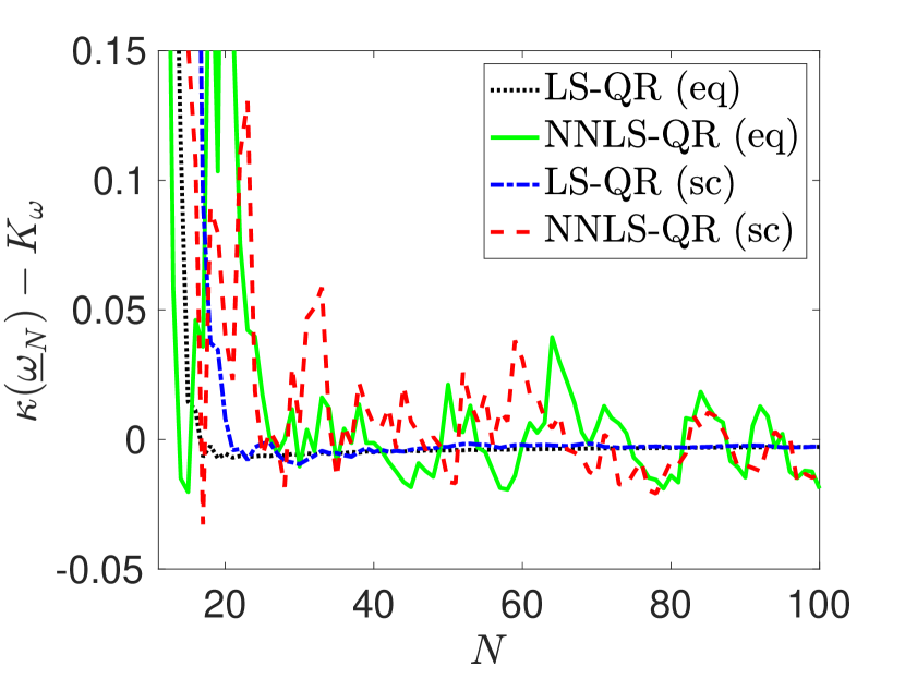
(a) ${\omega(x)=x\sqrt{1-x^{3}}}$

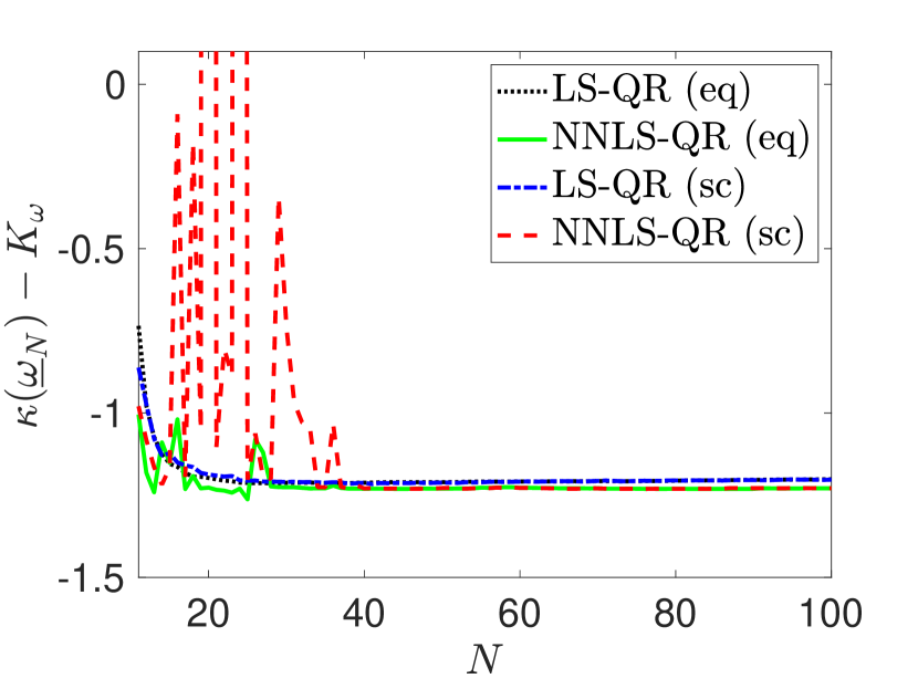
(b) ${\omega(x)=\cos(20\pi x)}$

Figure 1: Difference between the stability measure $\kappa(\underline{\omega}_{N})$ and the stability factor $K_{\omega}$ for the LS-QR and NNLS-QR for $d=10$, equidistant (eq) as well as scattered (sc) quadrature points, and two different weight functions $\omega$.

In accordance to Theorem 9 (and Theorem 11), we note that the stability measure for the LS-QR is bounded in all cases for increasing $N$. A similar behavior can be observed for the NNLS-QR on equidistant as well as scattered quadrature points. Yet, the NNLS-QR shows a slightly oscillatory profile in some tests. Finally, Figure 1 also demonstrates that in many cases the stability measure of the LS-QR and NNLS-QR is even lower than the one of the underlying integral $I$; see (1).

5.3 Sign-consistency

Next, we investigate sign-consistency of the proposed LS-QR and NNLS-QR. We measure sign-consistency by the following sign-consistency measure:

$$S_{\omega}(\underline{\omega}_{N})=\frac{1}{N}\sum_{n=1}^{N}\left|\operatorname{sign}(\omega_{n})-\operatorname{sign}(\omega(x_{n}))\right|.$$ (72)

It is evident that an $N$-point QR $Q_{N}$ with quadrature weights $\underline{\omega}_{N}$ is sign-consistent if and only if ${S_{\omega}(\underline{\omega}_{N})=0}$ holds.

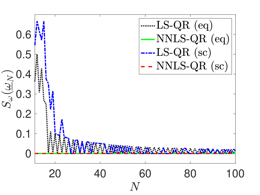
(a) $\omega(x)=x\sqrt{1-x^{3}}$

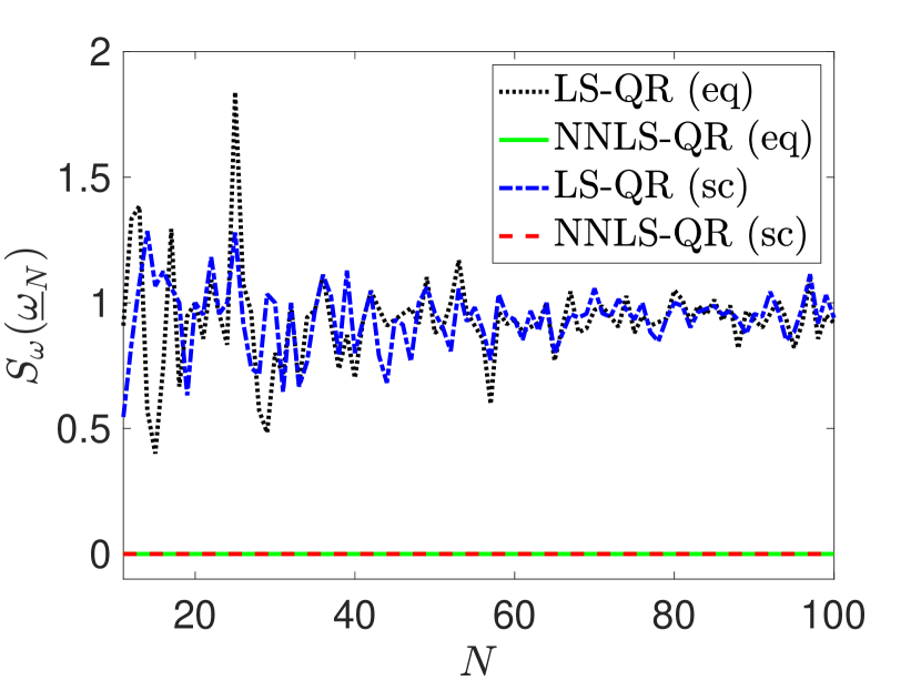
(b) $\omega(x)=\cos(20\pi x)$

Figure 2: Sign-consistency measure $S_{\omega}(\underline{\omega}_{N})$ for the LS-QR and NNLS-QR for $d=10$ and equidistant (eq) as well as scattered (sc) quadrature points.

Figure 2 illustrates the sign-consistency measure $S_{\omega}(\underline{\omega}_{N})$ for the LS-QR and the NNLS-QR for the two weight functions (70) with mixed signs, degree of exactness $d=10$, and equidistant as well as scattered quadrature points. We can observe that, in fact, the NNLS-QR always provides a sign-consistency measure of ${S_{\omega}(\underline{\omega}_{N})=0}$. The LS-QR, on the other hand, is demonstrated to violate sign-consistency in many cases. This indicates that the sign-consistent NNLS-QR might provide overall superior stability properties than the LS-QR.

5.4 Exactness

In this subsection, we investigate exactness of the LS-QR and the NNLS-QR. Figure 3 displays the exactness measure

$$\mathinner{\!\left\lVert A\underline{\omega}_{N}-\underline{m}\right\rVert}_{2}$$ (73)

of both QRs for the same set of parameters as before.

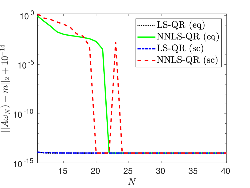
(a) $\omega(x)=x\sqrt{1-x^{3}}$

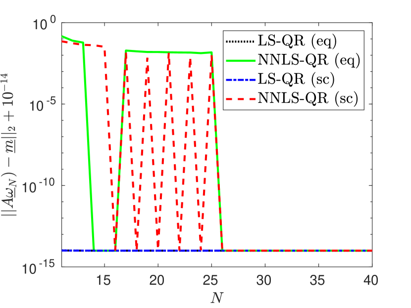
(b) $\omega(x)=\cos(20\pi x)$

Figure 3: Exactness measure $||A\underline{\omega}^{\mathrm{NNLS}}-\underline{m}||_{2}$ for the LS-QR and NNLS-QR for $d=10$, equidistant (eq) as well as scattered (sc) quadrature points, and two different weight functions.

Note that for an $N$-point QR $Q_{N}$ with quadrature weights $\underline{\omega}_{N}$ the minimal value for the exactness measure ${||A\underline{\omega}_{N}-\underline{m}||_{2}=0}$ holds if and only if $Q_{N}$ has degree of exactness $d$. In accordance to their construction as LS solutions of the linear system of exactness conditions (24), the LS-QR provides a minimal value of ${||A\underline{\omega}_{N}-\underline{m}||_{2}=0}$ in all cases. The NNLS-QR, on the other hand, violates the degree of exactness and are demonstrated to have a nonzero exactness measure if insufficiently small numbers of quadrature points $N$ are used. Yet, for fixed degree of exactness $d$ and increasing $N$, also the NNLS-QR provides degree of exactness $d$.

5.5 Accuracy for increasing $N$

We now come to investigate accuracy of the LS-QR and the NNLS-QR for a fixed degree of exactness $d=10$ and an increasing number of quadrature points $N$. We compare both QRs with a generalized composite trapezoidal rule applied to the unweighted Riemann integral with integrator $f\omega$. Further, we consider the two test functions $f(x)=|x|^{3}$ and $f(x)=e^{x}$. In the following, the errors

$$\left|Q_{N}[f]-I[f]\right|$$ (74)

are illustrated. Figure 4 shows the errors for equidistant quadrature points while Figure 5 provides the errors for scattered quadrature points. These are once more constructed by adding white Gaussian noise to the set of equidistant quadrature points; see (71).

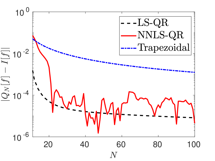
(a) $f(x)=|x|^{3}$ & $\omega(x)=x\sqrt{1-x^{3}}$

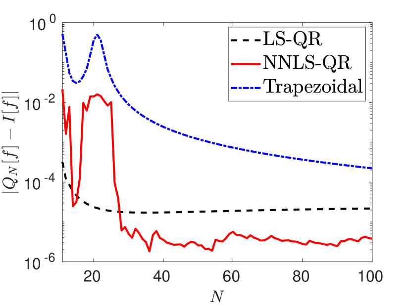
(b) $f(x)=|x|^{3}$ & $\omega(x)=\cos(20\pi x)$

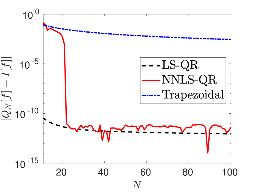
(c) $f(x)=e^{x}$ & $\omega(x)=x\sqrt{1-x^{3}}$

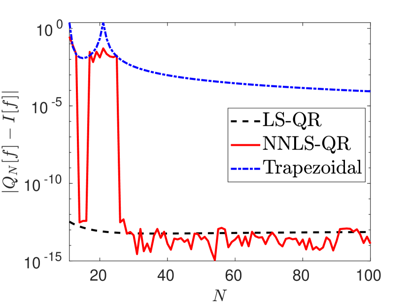
(d) $f(x)=e^{x}$ & $\omega(x)=\cos(20\pi x)$

Figure 4: Errors for the generalized composite trapezoidal rule, the LS-QR, and NNLS-QR with $d=10$ on equidistant points.

In Figure 4, where equidistant quadrature points are investigated, the LS-QR and NNLS-QR are demonstrated to provide more accurate results than the generalized composite trapezoidal rule in nearly all cases. In fact, both QRs yield highly accurate results which are up to $10^{12}$ times more accurate than the ones obtained by the generalized composite trapezoidal rule at the same set of quadrature points. Yet, the NNLS-QR is observed to oscillate in its accuracy and to be less accurate for small numbers of quadrature points $N$. Note that for an insufficiently large number of quadrature points $N$, the exactness condition (3) is not satisfied by the NNLS-QR, and therefore not even constants might be handled accurately. For a sufficiently large number of quadrature points, however, the NNLS-QR provides similar accurate (sometimes even more accurate) results as the LS-QR.

(a) $f(x)=|x|^{3}$ & $\omega(x)=x\sqrt{1-x^{3}}$

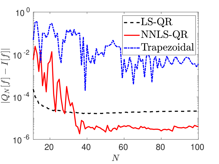
(b) $f(x)=|x|^{3}$ & $\omega(x)=\cos(20\pi x)$

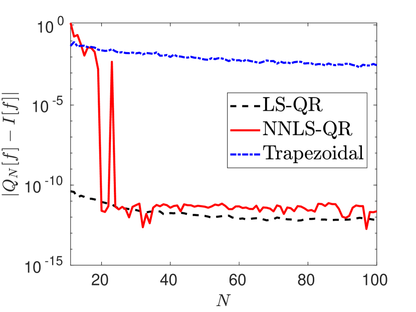
(c) $f(x)=e^{x}$ & $\omega(x)=x\sqrt{1-x^{3}}$

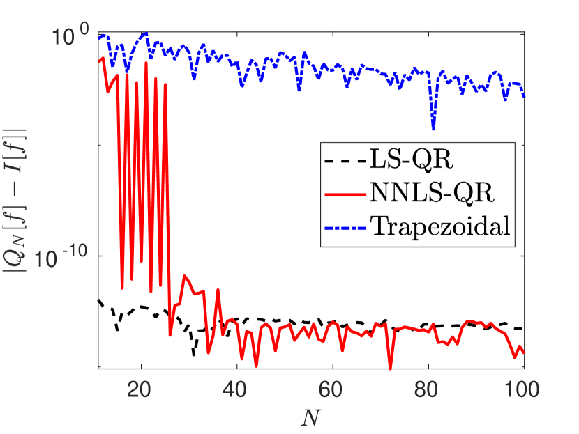
(d) $f(x)=e^{x}$ & $\omega(x)=\cos(20\pi x)$

Figure 5: Errors for the generalized composite trapezoidal rule, the LS-QR, and NNLS-QR with $d=10$ on scattered points.

Next, in Figure 5, we consider scattered quadrature points. For scattered quadrature points the results and differences between the different QRs become less clear. Yet, the LS-QR and the NNLS-QR are observed to provide more accurate results than the generalized composite trapezoidal rule in most cases. Note that even on scattered quadrature points both QRs are up to $10^{12}$ times more accurate. Yet, the oscillations in the accuracy of the NNLS-QR become more pronounced on scattered quadrature points. Again, the NNLS-QR is demonstrated to provide highly accurate results only when a sufficiently large number of quadrature points $N$ is used.

5.6 Accuracy for increasing $d$

In the last section, we have considered accuracy for fixed degree of exactness $d$ and an increasing number of quadrature points $N$. In this section, we investigate accuracy for an increasing degree of exactness $d$ and adaptively choose ${N=N(d)=\frac{1}{2}\left[(2d-1)^{2}+1\right]}$. This choice is motivated by Theorem 9. The most crucial step in the proof of Theorem 9 has been inequality (48), which holds for all ${k=0,\dots,d}$ if ${N\geq N(d)=\frac{1}{2}\left[(2d-1)^{2}+1\right]}$ is chosen.

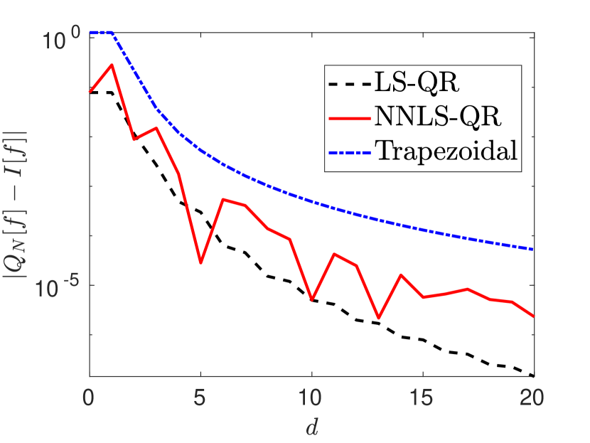
(a) $f(x)=|x|^{3}$ & $\omega(x)=x\sqrt{1-x^{3}}$

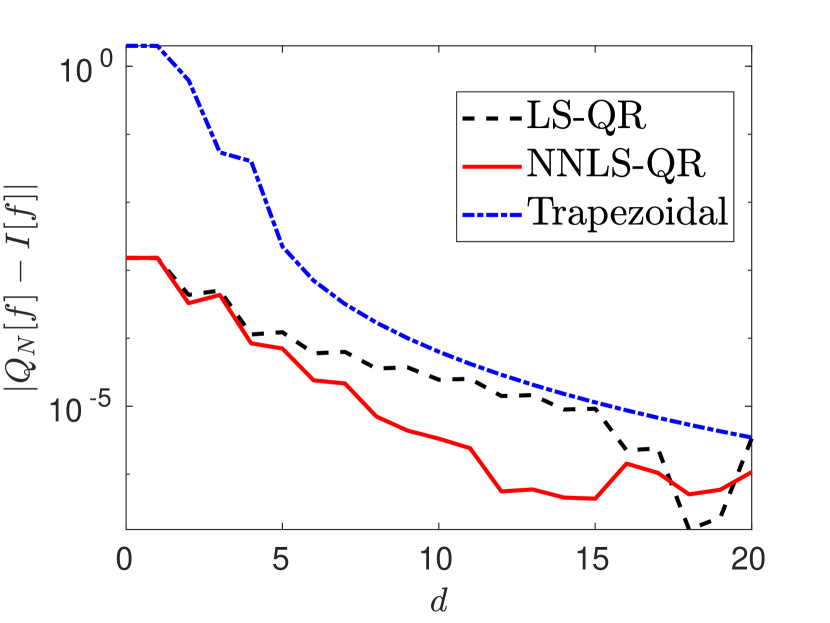
(b) $f(x)=|x|^{3}$ & $\omega(x)=\cos(20\pi x)$

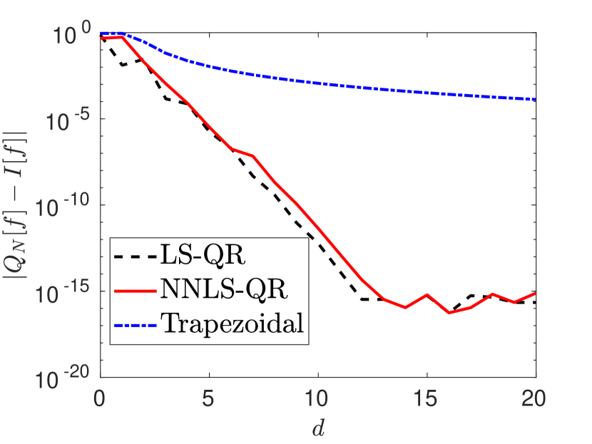
(c) $f(x)=e^{x}$ & $\omega(x)=x\sqrt{1-x^{3}}$

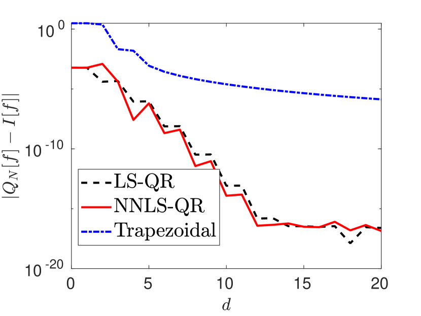
(d) $f(x)=e^{x}$ & $\omega(x)=\cos(20\pi x)$

Figure 6: Errors for the generalized composite trapezoidal rule, the LS-QR, and NNLS-QR on equidistant points.

Figure 6 illustrates the results of the LS-QR, the NNLS-QR, and the generalized composite trapezoidal rule for both test functions and weight functions as before on equidistant points. We observe that the LS-QR and the NNLS-QR provide more accurate results than the generalized composite trapezoidal rule in all cases. These are up to $10^{12}$ times more accurate. Yet, in that respect, it should be noted that the product $f\omega$ is either not analytic or not periodic for the weight functions $\omega$ and test functions $f$ considered here. Otherwise, i. e., if $f\omega$ was analytic and periodic, the composite trapezoidal rule would converge geometrically; see [25].

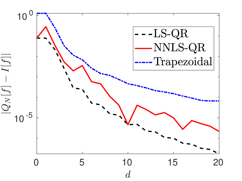
(a) $f(x)=|x|^{3}$ & $\omega(x)=x\sqrt{1-x^{3}}$

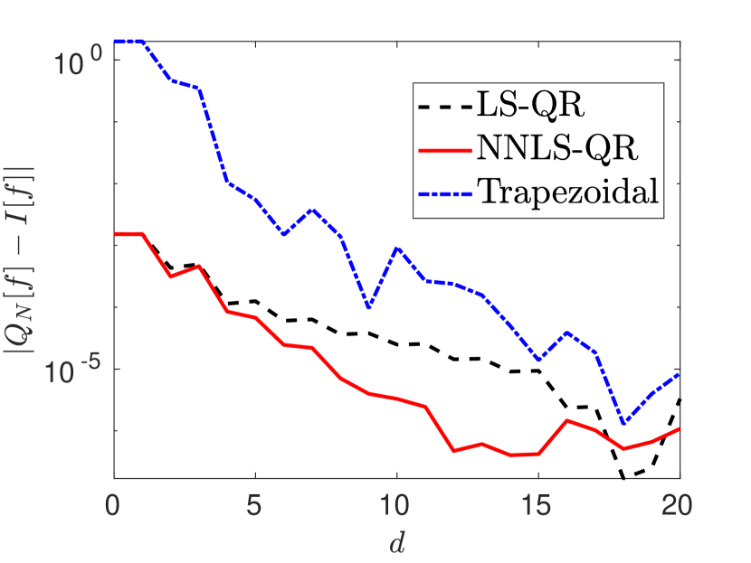
(b) $f(x)=|x|^{3}$ & $\omega(x)=\cos(20\pi x)$

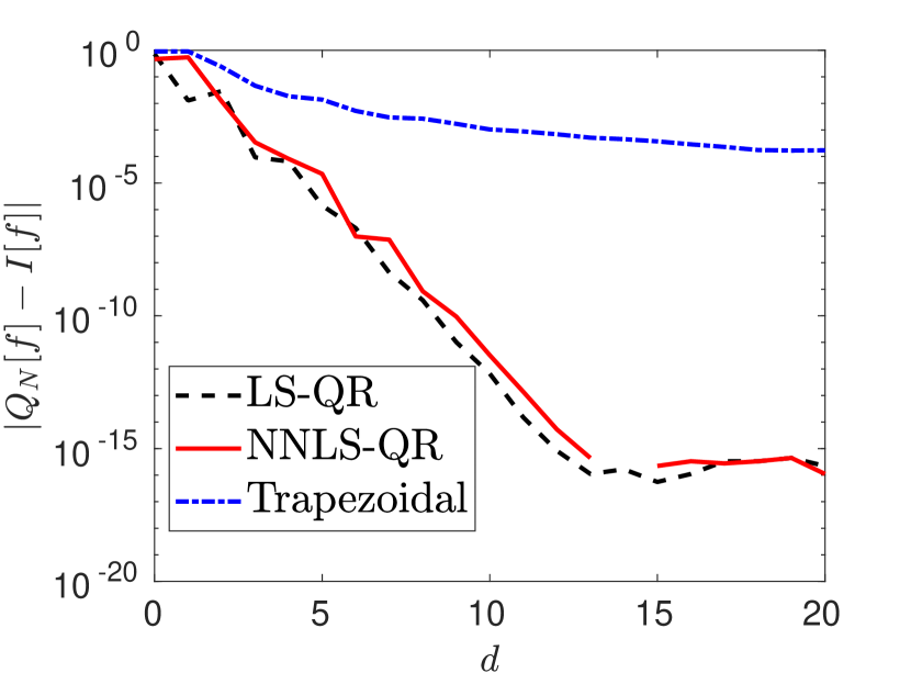
(c) $f(x)=e^{x}$ & $\omega(x)=x\sqrt{1-x^{3}}$

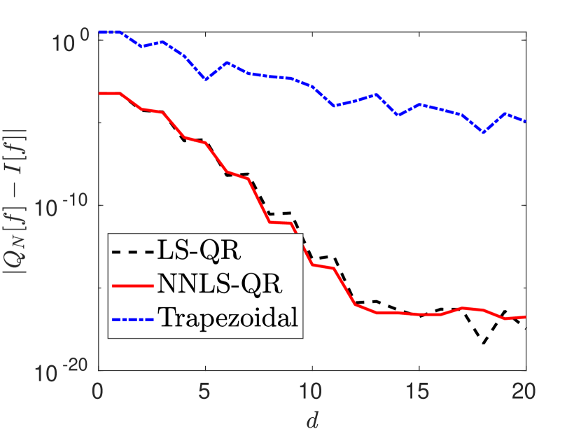
(d) $f(x)=e^{x}$ & $\omega(x)=\cos(20\pi x)$

Figure 7: Errors for the generalized composite trapezoidal rule, the LS-QR, and NNLS-QR on scattered points.

Similar observations can be made for scattered quadrature points and are displayed in Figure 7. Using the same set of equidistant or scattered quadrature points, the LS-QR and the NNLS-QR are able to provide highly accurate results even for general weight functions.

5.7 Ratio between $d$ and $N$

Finally, we address the ratio between the degree of exactness $d$ and the number of equidistant quadrature points $N$ that is needed for stability (and exactness) for the LS-QRs (and NNLS-QRs). In [26], Wilson showed that stability of LS-QRs for the weight function $\omega\equiv 1$ essentially is a $d^{2}$ process; that is, $N\approx Cd^{2}$ equidistant quadrature points are needed for $\kappa(\underline{\omega}_{N}^{\mathrm{LS}})=K_{\omega}$ to hold. In [15] and [11, Chapter 4], the same ratio between $d$ and $N$ has been observed for other positive weight functions, including $\omega(x)=1-x^{2}$ and $\omega(x)=\sqrt{1-x^{2}}$. Here, we demonstrate that a similar ratio also holds for more general weight functions.

$\omega(x)$	$1$	$1-x^{2}$	$\sqrt{1-x^{2}}$	$x\sqrt{1-x^{3}}$	$\cos(20\pi x)$
$s$	1.65	1.45	1.56	1.63	1.94
$C$	0.22	0.32	0.25	0.26	0.08

Table 1: LS fit of the parameters $C$ and $s$ in the model $N=Cd^{s}$ for the LS-QR and different weight functions $\omega$. $N$ refers to the minimal number of equidistant quadrature points such that the quadrature weights of the LS-QR with degree of exactness $d$ satisfy $\kappa(\underline{\omega}_{N}^{\mathrm{LS}})\leq 2K_{\omega}$.

$\omega(x)$	$1$	$1-x^{2}$	$\sqrt{1-x^{2}}$	$x\sqrt{1-x^{3}}$	$\cos(20\pi x)$
$s$	1.76	1.66	1.70	1.66	1.68
$C$	0.19	0.30	0.35	0.41	0.27

Table 2: LS fit of the parameters $C$ and $s$ in the model $N=Cd^{s}$ for the NNLS-QR and different weight functions $\omega$. $N$ refers to the minimal number of equidistant quadrature points such that the quadrature weights of the NNLS-QR with approximate degree of exactness $d$ satisfy $\kappa(\underline{\omega}_{N}^{\mathrm{NNLS}})\leq 2K_{\omega}$ as well as $||A\underline{\omega}_{N}^{\mathrm{NNLS}}-\underline{m}||_{2}\leq 10^{-14}$.

Table 1 lists the results of a LS fit of the parameters $C$ and $s$ in the model $N=Cd^{s}$ for the LS-QR and different weight functions $\omega$. Here, $N$ refers to the minimal number of equidistant quadrature points such that the quadrature weights of the LS-QR with degree of exactness $d$ satisfy $\kappa(\underline{\omega}_{N}^{\mathrm{LS}})\leq 2K_{\omega}$, where $d$ ranges from $0$ to $40$. Note that for general weight functions we have only been able to prove that $\kappa(\underline{\omega}_{N}^{\mathrm{LS}})$ is uniformly bounded w. r. t. $N$. Yet, in contrast to positive weight functions [11, Chapter 4], it is not ensured that $\kappa(\underline{\omega}_{N}^{\mathrm{LS}})\leq K_{\omega}$ holds for a sufficiently large $N$. In all numerical tests, we observed $\kappa(\underline{\omega}_{N}^{\mathrm{LS}})\leq 2K_{\omega}$ to hold for a sufficiently large $N$, however. In particular, this yields stability of the LS-QR. As a result of using $\kappa(\underline{\omega}_{N}^{\mathrm{LS}})\leq 2K_{\omega}$ instead of $\kappa(\underline{\omega}_{N}^{\mathrm{LS}})\leq K_{\omega}$ as a criterion to determine $N$, we observe slightly smaller exponent parameters $s<2$ in Table 1. Yet—and more important—we can note from Table 1 that the ratios between $d$ and $N$ are similar for positive and general weight functions. Similar ratios also hold for the NNLS-QR and are reported in Table 2. Here, $N$ refers to the minimal number of equidistant quadrature points such that the NNLS-QR with approximate degree of exactness $d$ (see §4) is stable as well as exact. Again, stability is checked by the condition $\kappa(\underline{\omega}_{N}^{\mathrm{NNLS}})\leq 2K_{\omega}$. Exactness, on the other hand, is checked by the condition $||A\underline{\omega}_{N}^{\mathrm{NNLS}}-\underline{m}||_{2}\leq 10^{-14}$. We use the bound $10^{-14}$ instead of $0$ to encounter possible round-off errors in our implementation; see §5.1.

6 Summary

In this work, we have investigated stability of quadrature rules for integrals with general weight functions, possibly having mixed signs. Such weight functions, for instance, arise in the weak form of the Schrödinger equation and for (highly) oscillatory integrals. In contrast to non-negative weight functions, stability of quadrature rules for general weight functions is not guaranteed by non-negative-only quadrature weights anymore. Therefore, we have proposed to treat stable quadrature rules (for which round-off errors due to inexact arithmetics are uniformly bounded with respect to the number of quadrature points $N$) and sign-consistent quadrature rules (for which the signs of the quadrature weights match the signs of the weight function at the corresponding quadrature points) as two separated classes.

Moreover, we have proposed two different procedures to construct such quadrature rules for general weight functions. In particular, our procedures allow us to construct stable high-order quadrature rules on equidistant and even scattered quadrature points. This is especially beneficial since in many applications it can be impractical, if not even impossible, to obtain data to fit known quadrature rules. Numerical tests demonstrate that both quadrature rules, referred to as least squares (LS-) and non-negative least squares quadrature rules (NNLS-QR), are able to provide highly accurate results.

Future work will focus on the extension of the proposed quadrature rules to higher dimensions.

Appendix: Discrete Chebyshev polynomials

The discrete Chebyshev polynomials arise as a special case of the Hahn polynomials [14, 22]. Also see [21, Chapter 18]. We collect some of their properties which come in useful in §3.4. For $\alpha,\beta>-1$ and $k=0,\dots,N-1$, the Hahn polynomials may be defined in terms of a generalized hypergeometric series as

$$Q_{k}(x;\alpha,\beta,N-1) ={}_{3}F_{2}(-k,-x,k+\alpha+\beta+1;\alpha+1,-N+1;1)$$ (75)

$$=\sum_{j=0}^{k}\frac{(-k)_{j}(k+\alpha+\beta+1)_{j}(-x)_{j}}{(\alpha+1)_{j}(-N+1)_{j}}\frac{1}{j!}$$

on $[0,N-1]$, where we have used the Pochhammer symbol

$$(a)_{0}=1,\quad(a)_{j}=a(a+1)\dots(a+j-1).$$ (76)

The Hahn polynomials are orthogonal on $[0,N-1]$ w. r. t. the inner product

$$\left\langle{f,\,g}\right\rangle_{\varrho}\mathrel{\mathop{\ordinarycolon}}=\sum_{n=0}^{N-1}f(n)g(n)\varrho(n)$$ (77)

with weight function

$$\varrho(x)\mathrel{\mathop{\ordinarycolon}}=\binom{x+\alpha}{x}\binom{N-1-x+\beta}{N-1-x}.$$ (78)

They are normalized by

$$\mathinner{\!\left\lVert Q_{k}(\cdot,\alpha,\beta,N-1)\right\rVert}_{\varrho}^{2}=h_{k}\mathrel{\mathop{\ordinarycolon}}=\frac{(-1)^{k}(k+\alpha+\beta+1)_{N}(\beta+1)_{k}k!}{(2k+\alpha+\beta+1)(\alpha+1)_{k}(-N+1)_{k}(N-1)!}.$$ (79)

Further, Dette [5] proved that for $\alpha+\beta>-1$ and

$$k\leq k(\alpha,\beta,N-1)\mathrel{\mathop{\ordinarycolon}}=-\frac{1}{2}\left(\alpha+\beta-1-\sqrt{(\alpha+\beta+1)(\alpha+\beta+2N-1)}\right)$$ (80)

the Hahn polynomials are bounded by

$$\max_{x\in[0,N-1]}\left|Q_{k}(x,\alpha,\beta,N-1)\right|\leq\max\left\{1,\frac{(\beta+1)_{k}}{(\alpha+1)_{k}}\right\}.$$ (81)

Here, we choose $\alpha=\beta=0$, which results in the discrete Chebyshev polynomials on $[0,N-1]$, and normalize and transform them to the interval $[a,b]$, resulting in the polynomials

$$\varphi_{k}\mathrel{\mathop{\ordinarycolon}}[a,b]\to\mathbb{R},\quad\varphi_{k}(x)=\frac{1}{\sqrt{h_{k}}}Q_{k}\left(\frac{N-1}{b-a}(x-a),0,0,N-1\right).$$ (82)

These polynomials form a basis of DOPs w. r. t. the original inner product $\left\langle{\cdot,\,\cdot}\right\rangle_{\underline{x}_{N}}$ in (32) when the points $\underline{x}_{N}$ are equidistant, i. e.,

$$x_{n}=b-a\frac{n-1}{N-1},\quad n=1,\dots,N.$$ (83)

Further, for

$$k\leq k(N)\mathrel{\mathop{\ordinarycolon}}=\frac{1}{2}\left(1+\sqrt{2N-1}\right)$$ (84)

they are bounded by

$$\max_{x\in[a,b]}\left|\varphi_{k}(x)\right|\leq\frac{1}{\sqrt{h_{k}}}.$$ (85)

Finally, we note that

$$(k+1)_{N} =\frac{(N+k)!}{k!},$$ (86)

$$(-N+1)_{k} =(-1)^{k}\frac{(N-1)!}{(N-k-1)!}.$$ (87)

Thus, we have

$$h_{k}=\frac{(-1)^{k}(k+1)_{N}k!}{(2k+1)(-N+1)_{k}(N-1)!}=\frac{(N+k)!(N-k-1)!}{(2k+1)(N-1)!(N-1)!}$$ (88)

for $\alpha=\beta=0$.

References

- [1] M. Abramowitz and I. A. Stegun. Handbook of Mathematical Functions: With Formulas, Graphs, and Mathematical Tables. National Bureau of Standards, Washington DC, 1964.
- [2] H. Brass and K. Petras. Quadrature Theory: The Theory of Numerical Integration on a Compact Interval. Number 178 in Math. Surveys and Monogr. American Mathematical Society, Providence, RI, 2011.
- [3] C. W. Clenshaw and A. R. Curtis. A method for numerical integration on an automatic computer. Numer. Math., 2(1):197–205, 1960.
- [4] P. J. Davis and P. Rabinowitz. Methods of Numerical Integration. Courier Corporation, North Chelmsford, MA, 2007.
- [5] H. Dette. New bounds for Hahn and Krawtchouk polynomials. SIAM Journal on Mathematical Analysis, 26(6):1647–1659, 1995.
- [6] L. Féjer. On the infinite sequences arising in the theories of harmonic analysis, of interpolation, and of mechanical quadratures. Bull. Amer. Math. Soc., 39(8):521–534, 1933.
- [7] W. Gautschi. Construction of Gauss–Christoffel quadrature formulas. Math. Comp., 22(102):251–270, 1968.
- [8] W. Gautschi. Numerical Analysis. Springer Science & Business Media, New York, NY, 1997.
- [9] W. Gautschi. Orthogonal Polynomials: Computation and Approximation. Oxford University Press, Oxford, UK, 2004.
- [10] A. Gelb, R. B. Platte, and W. S. Rosenthal. The discrete orthogonal polynomial least squares method for approximation and solving partial differential equations. Commun. Computat. Phys., 3(3):734–758, 2008.
- [11] J. Glaubitz. Shock Capturing and High-Order Methods for Hyperbolic Conservation Laws. Logos Verlag Berlin, Berlin, Germany, 2020.
- [12] J. Glaubitz and P. Öffner. Stable discretisations of high-order discontinuous Galerkin methods on equidistant and scattered points. Appl. Numer. Math., 151:98–118, 2020.
- [13] G. H. Golub and C. F. Van Loan. Matrix Computations. John Hopkins University Press, Baltimore, MD, 2012.
- [14] W. Hahn. Über Orthogonalpolynome, die q-Differenzengleichungen genügen. Mathe. Nachr., 2(1-2):4–34, 1949.
- [15] D. Huybrechs. Stable high-order quadrature rules with equidistant points. J. Comput. Appl. Math., 231(2):933–947, 2009.
- [16] D. Huybrechs and S. Olver. Highly oscillatory quadrature. In Highly Oscillatory Problems, pages 25–50. B. Engquist, A. Focus, E. Hairer, and A. Iserles, eds., Cambridge University Press, Cambridge, UK, 2009.
- [17] A. Iserles, S. Nørsett, and S. Olver. Highly oscillatory quadrature: The story so far. In Numerical Mathematics and Advanced Applications, pages 97–118. Springer, Berlin, 2006.
- [18] A. Iserles and S. P. Nørsett. On quadrature methods for highly oscillatory integrals and their implementation. BIT, 44(4):755–772, 2004.
- [19] V. I. Krylov and A. H. Stroud. Approximate Calculation of Integrals. Courier Corporation, North Chelmsford, MA, 2006.
- [20] C. L. Lawson and R. J. Hanson. Solving Least Squares Problems. SIAM, Philadelphia, PA, 1995.
- [21] F. W. J. Olver, A. B. Olde Daalhuis, D. W. Lozier, B. I. Schneider, R. F. Boisvert, C. W. Clark, B. R. Miller, B. V. Saunders, H. S. Cohl, and M. A. McClain. NIST Digital Library of Mathematical Functions. Release 1.0.26, March 15, 2020, 2020.
- [22] G. Szegö. Orthogonal Polynomials. American Mathematical Society, Providence, RI, 1939.
- [23] L. N. Trefethen. Is Gauss quadrature better than Clenshaw–Curtis? SIAM Review, 50(1):67–87, 2008.
- [24] L. N. Trefethen and D. Bau III. Numerical Linear Algebra. SIAM, Philadelphia, PA, 1997.
- [25] L. N. Trefethen and J. Weideman. The exponentially convergent trapezoidal rule. SIAM Review, 56(3):385–458, 2014.
- [26] M. W. Wilson. Discrete least squares and quadrature formulas. Math. Comp., 24(110):271–282, 1970.
- [27] M. W. Wilson. Necessary and sufficient conditions for equidistant quadrature formula. SIAM Journal on Numerical Analysis, 7(1):134–141, 1970.