Cosmic ray propagation in the Universe in presence of a random magnetic field
Abstract
The origin of the ultrahigh energy cosmic ray remains being a mystery. However, a considerable progress has been made in the past few years due to the good quality data recorded by current cosmic ray observatories. One of the recent achievements is obtaining firm observational evidence about the extragalactic origin of the most energetic cosmic rays by the Pierre Auger observatory. On the other hand, it is believed that there is a non-null turbulent magnetic field that fills the intergalactic medium. Therefore, the presence of the intergalactic magnetic field can play an important role on the propagation of the ultrahigh energy cosmic rays through the Universe, which in principle can be relevant to interpret the experimental data. In this work we present a system of partial differential equations that describes the propagation of the ultrahigh energy cosmic rays through the Universe, in the presence of a turbulent intergalactic magnetic field, that includes the diffusive and the ballistic regime of propagation and also the transition between them. Also, as an example of application, the system of equations is solved numerically in a simplified physical situation.
1 Introduction
Despite the significant progress made in recent years, especially in the field of experimental research, the origin and nature of the ultrahigh energy cosmic rays (UHECRs, eV) are still unknown. The Pierre Auger Observatory, located in the southern hemisphere, and Telescope Array, located in the northern hemisphere, are currently taking data of very good quality. Also the current statistics is quiet large, specially the one corresponding to Auger which at present has accumulated a very large exposure.
The UHECR flux has been measured with unprecedented statistics by Auger and Telescope Array. It presents two main features, a hardening at eV, known as the ankle and a suppression. This suppression is observed by Auger at eV and by Telescope Array at a larger energy, eV [1]. Also, the Auger spectrum takes smaller values than the ones corresponding to Telescope Array. The discrepancies between the two observations can be diminished by shifting the energy scales of both experiments within their systematic uncertainties. However, some differences are still present in the suppression region [1].
It has long been believed that the most energetic part of the UHECR flux is of extragalactic origin. This is due to the known inefficiencies of the galactic sources to accelerate particles at the highest energies. Moreover, very recently Auger has found strong observational evidence about the extragalactic origin of the cosmic rays with primary energies above eV from the study of the distribution of their arrival directions. Considering this data set an anisotropy that can be described as a dipole of % amplitude was found [2]. The significance of this detection is larger than and the dipole direction is such that a scenario in which the flux is dominated by a galactic component is disfavored [2].
The transition between the galactic and extragalctic components is still an open problem of the high energy astrophysics. The Auger data show that the large scale distribution of the cosmic ray arrival directions is compatible with an isotropic flux, in the energy range from eV up to the ankle [3]. This result is incompatible with a galactic origin of the light component that seems to dominate the flux in this energy range [3]. Therefore, the transition between these two components is expected to take place below eV.
Thus, the large scale arrival direction analyses done by Auger, combined with the composition information at lower energies, shows that the UHECR flux seems to be dominated by the extragalactic component.
It is believed that the intergalactic medium is filled with a turbulent magnetic field, which affects the propagation of the charged extragalactic UHECRs through the Universe. In particular, the effects produced on the propagation of charged nuclei are relevant to explain the UHECR data (see refs. [4, 5] for recent works).
The propagation of charged particles in a random magnetic field depends on the distance traveled by the particles under the influence of the field compared with the scattering length , where is the diffusion coefficient and is the speed of light. For traveled distances much smaller than , which in general corresponds to the region close to the source, the propagation is ballistic. For traveled distances much larger than , the propagation is diffusive (see, for instance, ref. [6]).
The propagation of the UHECRs in the presence of the intergalactic magnetic field can be study from simulations [7] or through the appropriated transport equation that describes this physical problem. In ref. [8] a partial differential equation is obtained for the number density of particles which is valid for the diffusive regime of propagation. This equation can be solved analytically provided the diffusion coefficient for a given random magnetic field model. A phenomenological extension of the solution found in ref. [8] to the ballistic case is proposed in ref. [9].
On the other hand, in ref. [10] a system of partial differential equations is obtained applying the method of moments to the Boltzmann equation with an appropriated collision term introduced to describe the propagation of cosmic rays generated in galactic sources, for which the effects of the expansion of the Universe are negligible. In this case the equations system is formed by two coupled partial differential equations for the number density of particles and the flux. These equations take into account the ballistic and the diffusive regimes of propagation and also the transition between both of them. Also, an analytic solution of this equations system is found for the stationary case. In this work we find a system of partial differential equations also for the number density of particles and the flux applying the methods of moments to the Boltzmann equation, which includes both, the effects of the intergalactic magnetic field and the expansion of the Universe. In this case, the starting point is the Boltzmann equation in a curved space-time. We also solve numerically the equations system for a simplified physical situation which shows that the equations found properly describe the ballistic and the diffusive regime of propagation and also the transition between them.
2 The transport equation and the method of moments
The propagation of the cosmic rays in the expanding Universe is described by the Boltzmann equation in a curved space-time. The Friedmann-Lemaître-Robertson-Walker (FLRW) metric for a spatially flat Universe is considered,
| (2.1) |
where are comoving coordinates with , is the scale factor, and is the Kronecker delta function with . In eq. (2.1) and in the rest of the article the speed of light is considered.
The geodesic equation is given by,
| (2.2) |
where is the four-momentum of the particle, is the affine parameter, and are the Christoffel symbols. For the FLRW metric the non-null Christoffel symbols are: and , where and is the Hubble parameter. The geodesic equation for the spatial components of the four-momentum and for the FLRW metric takes the following form,
| (2.3) |
It is appropriated to work in the local inertial frame, which corresponds to an observer placed at a point with space-time coordinates [11]. It is worth mentioning that in this frame the collision term of the Boltzmann equation takes the same form as in Special Relativity. The tangent space associated to a given space-time point is spanned by a basis of four contravariant vectors which are called the tetrad. The choice of the tetrad defines the reference frame in that point. The natural tetrad is the one known as the coordinate tetrad, which corresponds to the directional derivatives with respect to the coordinates. The tetrad corresponding to the local inertial frame is the one in which the metric takes the form of the one corresponding to the Minkovski space-time. Therefore, the four-momentum in the local inertial frame takes the following form (see for instance ref. [12]),
| (2.4) |
Note that in the local inertial frame the relationship between the energy of a particle and the momentum is , where . For massless particles or in the case where , .
The equation fulfilled by the spatial components of the four-momentum in the local inertial frame is obtained from eqs. (2.3) and (2.4),
| (2.5) |
where .
The Boltzmann equation in a curved space-time is given by [11],
| (2.6) |
where is the collision term and is a source term. Here the function depends on the space-time coordinates of a point and on the spatial coordinates of the four-momentum in the local inertial frame, i.e. where and .
By using eq. (2.5) the Boltzmann equation becomes,
| (2.7) |
where is a unit vector pointing in the direction of motion of the particles, , and .
The collision term considered is the one introduced in ref. [10],
| (2.8) |
where is the scattering probability for a particle with initial direction of motion and final direction of motion per unit of time at the point . Note that it assumed that , which corresponds to the case where , a very good approximation for UHECRs.
The source term considered is the following,
| (2.9) |
which corresponds to a point source placed at that started to emit cosmic rays at . Here is the delta Dirac function and is the Heaviside function.
The four-current in the local inertial frame is given by [12],
| (2.10) |
Therefore, the number density of particles and the flux differential in energy are given by,
| (2.11) | ||||
| (2.12) |
Following ref. [10], after applying the integral operators and to eq. (2.7), the equations for the number density of particles and the flux are obtained,
| (2.13) | ||||
| (2.14) |
where , in which the term is included to take into account processes modeled as continuous energy losses of the particles. Here,
| (2.15) | ||||
| (2.16) |
where is the isotropization tensor. Note that these expressions are the same as the ones obtained in ref. [10]. The assumptions to obtain eqs. (2.13), (2.14), (2.15), and (2.16) are: , the source term does not depends on , i.e. which corresponds to a source emitting cosmic rays isotropically, and .
It is worth mentioning that, the number density of particles and the flux are related to observable physical quantities [13] (see also refs. [14] and [15]). Following ref. [13], the cosmic ray intensity can be written as,
| (2.17) |
where points to a given direction in the sky and corresponds to terms with of the multipole expansion. Therefore, is proportional to the average cosmic ray intensity over the entire sky and is related to the dipole vector, which is defined as [13],
| (2.18) |
The dipole amplitude is given by the norm of the dipole vector, i.e. . The dipole vector can be reconstructed from the distribution of the arrival directions of the UHECRs [2].
In the diffusive regime the first three terms of eq. (2.14) can be discarded and also since , the following expression for the flux as a function of the number density of particles is obtained,
| (2.19) |
where is the diffusion coefficient. Introducing eq. (2.19) in eq. (2.13) the equation for the number density of particles of ref. [8] is obtained. Therefore, the number density of particles obtained solving eqs. (2.13) and (2.14) has to be approximately equal to the analytic solution found in ref. [8] when the diffusive limit is considered.
Note that, the equations system of ref. [10] is obtained introducing and in equations (2.13) and (2.14). Also note that the source term in eq. (2.13) is different than the one of ref. [10] due to the different physical scenario considered in this work.
Let us consider the case in which the cosmic ray source is at the coordinates origin and that there is spherical symmetry. Under these assumptions the number density of particles and the flux depend only on the radial coordinate and the flux has a non-null component in the radial direction, , only. Also, following ref. [10], it is assumed that the isotropization tensor has the following shape,
| (2.20) |
where is the isotropization function and .
The equations for the number density of particles and the radial component of the flux, , are given by,
| (2.21) | ||||
| (2.22) |
In order to simplify the equations for and a change of the variable to a new variable is performed. The new variable is obtained by solving the following equation,
| (2.23) |
with the condition where is taken as the age of the Universe. In this way a function is obtained, which corresponds to the energy that a particle has to have at time in order to be observed at time with energy . This change of variable is such that the partial derivative with respect to does not appear in the equations for and . Note that this change of variable is the same as the one that appears in the method of characteristics used to solve systems of partial differential equations [16]. Therefore, introducing this change of variable and considering the following functions,
| (2.24) | ||||
| (2.25) |
a new equations system for and is obtained,
| (2.26) | ||||
| (2.27) |
Here the energy variable in the functions , , and is replaced by the function . The functions and have to be given as function of the variable and not . After solving the eqs. (2.26) and (2.27) the change of variables from to has to be done. However, if the solutions are evaluated at time the change of variable is not necessary, since .
The extragalactic magnetic field is poorly known (see ref. [17] for a review). Measurements of the magnetic field intensity in galaxy clusters suggest that the magnetic field intensity in high density regions like sheets and filaments can reach values up to few G. In contrast, observational constraints show that the magnetic field intensity in voids is smaller than nG. Therefore, the extragalactic magnetic field can have a strong dependence on , which is translated into a strong dependence of the isotropization tensor and the diffusion coefficient on . While, the equations system composed by eqs. (2.13) and (2.14) describes the general situation in which both the isotropization tensor and the diffusion coefficient can have a general dependence on , the equations system given by eqs. (2.26) and (2.27) is valid for models of the intergalactic magnetic field with spherical symmetry, in particular the simple one in which the intergalactic magnetic field is isotropic and homogeneous.
It is worth mentioning that the equations system obtained can be very useful in the context of semi-analytical methods used to include the effects of the intergalactic magnetic field in models of the UHECR flux like the ones developed in refs. [18, 4, 5].
Furthermore, the equations system formed by the and functions can be extended in order to include several nuclear species and also the photodisintegration and photopion production processes undergone by the nuclei during propagation through the radiation field present in the Universe. This extension, that will be discussed in a forthcoming article, can be important for the development of models of the UHECR flux that include the effects of the intergalactic magnetic field. Note that this type of formalism can reduce considerably the computation time compared to the methods based on Monte Carlo simulations.
3 A simple example
Let us consider a simplified case in which a source emits ultrahigh energy protons isotropically, which lose energy due to the adiabatic expansion of the Universe only (i.e. ) when they propagate through the Universe. Let us also consider that the extragalactic magnetic field is modeled as an isotropic and homogeneous random field such that . Note that this is a simplified model of the intergalactic magnetic field (see section 2). Therefore, under these assumptions the propagation of the protons is described by eqs. (2.26) and (2.27). It is also assumed that the source emits cosmic rays at a constant rate in comoving volume with a spectrum that follows a power law in energy, , where with a constant and the spectral index.
Since the particles propagate without interacting . Introducing this expression in eq. (2.23) and solving the differential equation with the corresponding condition, the following expression for the energy as a function of time and is obtained, , where since is chosen as the age of the Universe it follows that .
The exponential factor on the right-hand side of eq. (2.26) is given by,
| (3.1) |
in which it is used that .
Rescaling the function and from eqs. (2.26) and (2.27) such that and the following equations are obtained,
| (3.2) | ||||
| (3.3) |
Note that for these two function are related to and through the following expressions,
| (3.4) | ||||
| (3.5) |
where is the enhancement factor introduced in ref. [4]. Also, note that from eq. (2.18) it can be seen that the dipole amplitude is given by,
| (3.6) |
In the general case eqs. (3.2) and (3.3) cannot be solved analytically (an analytic solution can be found for the ballistic regime where , see appendix A). Therefore, the equations system is solved numerically by using the finite differences method [20].
The diffusion coefficient used in the numerical calculation is taken from ref. [6], which is given by,
| (3.7) |
where is the coherent length of the random magnetic field. Here , where is the charge number of the nucleus, is the absolute value of the electron charge, and is the root mean square of the random magnetic field. This expression corresponds to the type of turbulence given by the Kolmogorov spectrum.
The scale factor and the Hubble parameter considered for the calculation are given by [19],
| (3.8) | ||||
| (3.9) |
where km s-1 Mpc-1 is the Hubble constant, and are the density parameters for matter and dark energy, respectively.
Motivated by ref. [10], the isotropization function is assumed to have the following expression, , where is a very slowly decreasing function of energy that ranges from 1.65 at eV to 0.935 at eV. The function is determined in such a way that the numerical solutions and have the form corresponding to the ballistic regime of propagation for . Note that exact shape of the isotropization function is unknown, further studies are required to determine it.
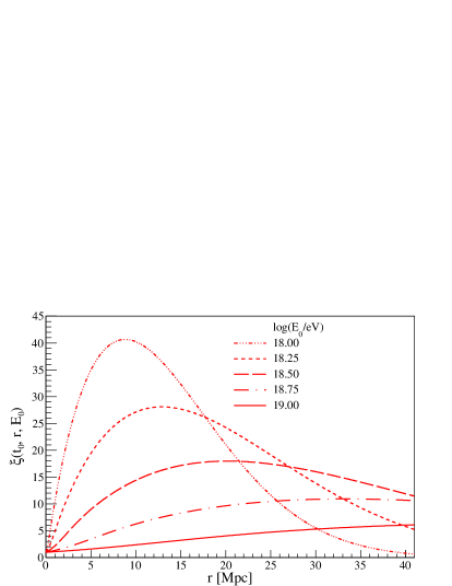
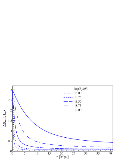
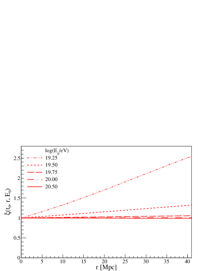
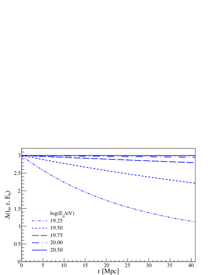
Figure 1 shows and as a function of for , corresponding to redshift , nG, Mpc, and for different values of . At eV the propagation is done mainly in the diffusive regime since ranges from 0.32 Mpc at to 0.26 Mpc at . The diffusive character of the propagation can be seen at the upper panels of the figure. As the energy increases also increases in such a way that at eV, it ranges from Mpc at to Mpc at . Therefore, for increasing values of the energy and . These limit values correspond to the ballistic propagation regime. As can be seen from the figure, for increasing values of energy and tend to the solution found for the ballistic regime of propagation which is studied in detail in Appendix A. This is clearly seen from the bottom-left panel of the figure where tends to one for distances relatively close to . From the bottom-right panel of the figure, it can also be seen that the dipole amplitude as a function of tends to the constant function , which corresponds to what is expected for the ballistic propagation regime.
4 Conclusions
The effects of the turbulent intergalactic magnetic field on the propagation of the ultrahigh energy cosmic rays can play a very important role to explain current experimental data. Motivated by this fact, we have studied the propagation of the ultrahigh energy cosmic rays in presence of the turbulent intergalactic magnetic field, considering the Boltzmann equation in a curved space-time, to take into account the expansion of the Universe. Considering the moments of the distribution we have obtained a system of partial differential equations for the number density of particles and for the flux that take into account the ballistic and the diffusive regimes of propagation as well as the transition between them. We have found that in both, the diffusive and ballistic limits, the known solutions are recovered. Finally, we have solved numerically the equations system for a simplified case in which it can be clearly seen the transition from the diffusive to the ballistic regimes of propagation as the energy measured at a given comoving distance from the source increases.
It is worth mentioning that the equations system found can be extended in order to include the propagation of different nuclear species with their respective interactions (photodisintegration and photopion production) in the radiation field present in the Universe. This can be used for the development of models of the ultrahigh energy cosmic ray flux that include the effect of the intergalactic magnetic field.
Appendix A Analytic solution for the ballistic regime of propagation
In the ballistic regime and , then eqs. (3.2) and (3.3) become,
| (A.1) | ||||
| (A.2) |
Eqs. (A.1) and (A.2) can be solved by using the method of characteristics [16]. The solution is such that , where
| (A.3) |
Here,
| (A.4) |
is the comoving distance traveled by a massless particle that is injected at at time , is the inverse function of , and . Note that for it follows that .
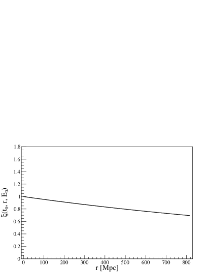
The left panel of fig. 2 shows as a function of from to for the same parameters used in the full numerical calculation of section 3, i.e. and . From the left panel of the figure it can be seen that decreases with . This is due to the fact that the protons that reach larger values of with energy at time have to be injected by the source with larger energies, due to the adiabatic energy loss undergone by them during propagation. The more energetic particles are less numerous due to the decrease of the energy spectrum with energy. From the right panel of the figure it can be seen that for it follows that .

In the ballistic regime of propagation the dipole amplitude is given by eq. (3.6), which gives due to the fact that, in this case, .
Acknowledgments
A. D. S. is member of the Carrera del Investigador Científico of CONICET, Argentina. This work is supported by ANPCyT PICT-2015-2752, Argentina. The author thanks the members of the Pierre Auger Collaboration, specially R. Clay for reviewing the manuscript.
References
- [1] D. Ivanov, Report of the Telescope Array - Pierre Auger Observatory Working Group on Energy Spectrum, PoS ICRC2017 (2018) 498.
- [2] Pierre Auger collaboration, Observation of a Large-scale Anisotropy in the Arrival Directions of Cosmic Rays above eV, Science 357 (2017) 1266 [arXiv:1709.07321].
- [3] Pierre Auger collaboration, Large scale distribution of arrival directions of cosmic rays detected above eV at the Pierre Auger Observatory, Astrophys. J. Suppl. 203 (2012) 34 [arXiv:1210.3736].
- [4] S. Mollerach and E. Roulet, Ultrahigh energy cosmic rays from a nearby extragalactic source in the diffusive regime, Phys. Rev. D 99 (2019) 103010 [arXiv:1903.05722].
- [5] S. Mollerach and E. Roulet, Extragalactic cosmic rays diffusing from two populations of sources, Phys. Rev. D 101 (2020) 103024 [arXiv:2004.04253].
- [6] D. Harari, S. Mollerach and E. Roulet, Anisotropies of ultrahigh energy cosmic rays diffusing from extragalactic sources, Phys. Rev. D 89 (2014) 123001 [arXiv:1312.1366].
- [7] R. Alves Batista, A. Dundovic, M. Erdmann, K.-H. Kampert, D. Kuempel, G. Müller et al., CRPropa 3 - a Public Astrophysical Simulation Framework for Propagating Extraterrestrial Ultra-High Energy Particles, JCAP 05 (2016) 038 [arXiv:1603.07142].
- [8] V. Berezinsky and A.Z. Gazizov, Diffusion of cosmic rays in expanding universe, Astrophys. J. 643 (2006) 8 [astro-ph/0512090].
- [9] R. Aloisio, V. Berezinsky and A. Gazizov, Superluminal problem in diffusion of relativistic particles and its phenomenological solution, Astrophys. J. 693 (2009) 1275 [arXiv:0805.1867].
- [10] A.Y. Prosekin, S.R. Kelner and F.A. Aharonian, On transition of propagation of relativistic particles from the ballistic to the diffusion regime, Phys. Rev. D 92 (2015) 083003 [arXiv:1506.06594].
- [11] G. Pettinari, The Intrinsic Bispectrum of the Cosmic Microwave Background, Springer International Publishing, Cham, Switzerland (2016).
- [12] J. Bernstein, Kinetic Theory in the Expanding Universe, Cambridge University Press, Cambridge, U.K. (1988).
-
[13]
M. Ahlers and P. Mertsch, Origin of Small-Scale Anisotropies in Galactic
Cosmic Rays,
Prog. Part. Nucl. Phys. 94 (2017) 184 [arXiv:1612.01873]. -
[14]
M. Ahlers, Anomalous Anisotropies of Cosmic Rays from Turbulent Magnetic
Fields,
Phys. Rev. Lett. 112 (2014) 021101 [arXiv:1310.5712]. - [15] O. Deligny, Measurements and implications of cosmic ray anisotropies from TeV to trans-EeV energies, Astropart. Phys. 104 (2019) 13 [arXiv:1808.03940].
- [16] I. Stavroulakis and S. Tersian, Partial Differential Equations An Introduction with Mathematica and MAPLE (Second Edition), World Scientific, New Jersey, U.S.A. (2004).
- [17] J.L. Han, Observing Interstellar and Intergalactic Magnetic Fields, Annu. Rev. Astron. Astrophys. 55 (2017) 111.
- [18] S. Mollerach and E. Roulet, Magnetic diffusion effects on the ultra-high energy cosmic ray spectrum and composition, JCAP 10 (2013) 013 [arXiv:1305.6519].
- [19] E. Kolb, M. Turner, The Early Universe, Addison-Wesley, Redwood, U.S.A. (1988).
- [20] J. Thomas, Numerical Partial Differential Equations: Finite Difference Methods, Springer, New York, U.S.A. (1995).