Capacity Value of Solar Power and Other Variable Generation

Abstract

This paper reviews methods that are used for adequacy risk assessment considering solar power and for assessment of the capacity value of solar power. The properties of solar power are described as seen from the perspective of the power-system operator, comparing differences in energy availability and capacity factors with those of wind power. Methodologies for risk calculations considering variable generation are surveyed, including the probability background, statistical-estimation approaches, and capacity-value metrics. Issues in incorporating variable generation in capacity markets are described, followed by a review of applied studies considering solar power. Finally, recommendations for further research are presented.

I Introduction

Akey issue for power-system planning is the contribution of renewable and other emerging energy resources to meeting demand reliably. Mechanical failures, planned maintenance, or lack of generating resource in real-time may leave a system with insufficient capacity to meet load—requiring load curtailment. The contribution of a resource to serving demand reliably is measured typically by estimating capacity-value metrics, defined through the effect that its addition to the system has on the calculated risk of load-curtailment events. The issue of real-time resource availability is particularly salient with renewable resources, as their output is governed by uncontrollable weather conditions.

An IEEE Task Force focused on techniques for estimating the capacity value of wind power published a survey on that technology [1]. This new paper has a similar purpose of surveying methods for estimating the capacity value of solar power and recent activity applicable to both wind and solar. We place strong emphasis on critical review of modelling methodology, particularly with respect to capacity markets and statistical modelling, which distinguishes our review work from related publications [1, 2, 3]. The paper builds on earlier Task Force papers which concentrate more specifically on solar power [4, 5]—while the high-level topics covered in this new paper are broadly similar to those in a previous conference paper [5], the material is revised entirely for this as the Task Force’s final report apart from Sections III-A–III-C (these cover the essentials of the relevant probabilistic and statistical modelling, where the Task Force’s thinking has evolved less rapidly.) Throughout the Task Force’s activity, there is particular emphasis on matters of solar-resource assessment (with which the power-system community may be less familiar as compared to wind). In the solar-specific sections, we focus on photovoltaic (PV) solar rather than concentrating solar power (CSP). CSP has intrinsic energy-storage capability [6, 7], providing some control of co-incidence of output with high demands. This characteristic of CSP makes relevant modelling approaches fundamentally different from PV. A brief discussion regarding the interaction between solar power and co-located energy storage, which is applicable to CSP, is given in Section III-F.

This paper addresses four major issues that are related to solar power. First, Section II discusses key properties and assessment of solar resource. Solar availability features unique spatial and temporal correlations, which are modified by design considerations such as panel orientation and the inclusion of sun-tracking systems or energy storage. Section III provides a detailed discussion of the statistical methods that are used for adequacy-index and capacity-value estimation—much of which applies equally to other variable generation (VG) technologies, as well as solar. We highlight the importance of capturing statistical relationships between renewable resource and demand, and consequences of limited data. It discusses also relevant theory associated with capacity markets. Section IV surveys recent capacity value studies and practice in the industrial and research literature, emphasising consequences of different methodology choices. Finally, Section V concludes and discusses key research needs in this area.

II PV-Resource Assessment

Surface solar irradiance follows predictable diurnal and seasonal cycles. However, solar irradiance can be difficult to model and forecast, due to cloud cover and other meteorological effects. The recent emergence of PV and its distributed nature make reliable long-term output data rare, forcing reliance on modeled PV-generation data [8]. Weather variability occurs at different temporal and spatial scales, from clouds moving across individual panels (seconds to minutes [9]) to weather fronts moving over a region (hours to days [10]) to multi-day regimes that dictate continental-scale weather patterns [11]. Fig. 1 demonstrates the variability in PV output at a single location over short timescales and that this variability is reduced if many PV systems over a wide area are aggregated.

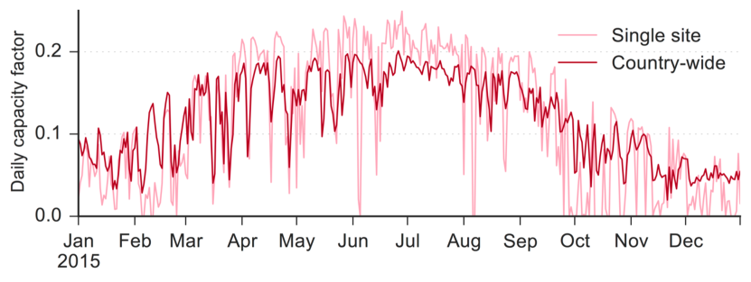
Figure 1: Daily-average capacity factor for a single PV system near Milan and for PV deployed across Italy during $2015$. Single-site and Italy-wide data are from PVOutput and Terna, respectively.

Modelling PV power output accurately is hampered by the difficulty of estimating solar irradiance [12], especially due to cloud cover. Aerosols and other atmospheric particles scatter incoming light even with clear skies [13], affecting the productivity of concentrating technologies (CSP and concentrating PV) and, to a lesser degree, PV. Moreover, deposition of aerosols and particles on panels affects productivity [14]. Output depends also on many secondary parameters: the PV technology that is used, tilt and azimuth angles, whether panels are fixed or have tracking systems, module temperature [15], and panel shading as a function of sun angle [16]. Fig. 2 illustrates the impact of orientation on PV output, using data for Jaen, Spain. Other weather variables play a role as well: the severity of soiling is mediated by rainfall [17] and snow can cover panels (reducing output) and reflect sunlight off the ground (increasing output) [18]. Finally, a PV system’s inverter determines AC power output, with an efficiency that depends on utilization (power level and input voltage) and operating temperature [19]. It is common for inverters to be undersized relative to peak DC output of a panel, giving flattened power-output peaks. While this affects summer peak output in particular, snow affects winter peaks. PV output during both summer and winter peaks contribute to the capacity value of a PV system.

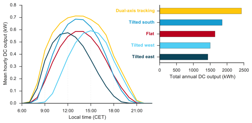
Figure 2: Simulated power generation for a $1$-kW system installed in Jaen, Spain, averaged hourly over all days of $2015$ (left) and summed over the entire year (right). The tilted systems are installed at $35$-degree tilt angle, facing exactly south, east, or west. Data from https://www.renewables.ninja.

II-A Calculating Power Output

A key challenge in modeling overall system performance is obtaining accurate irradiance data. Several methods exists to convert irradiance to DC power output from PV panels. Common approaches are empirical models, which are parameterized from manufacturer datasheets, and experimental data [20, 15]. The two primary weather inputs—module irradiance and temperature—are modified by the secondary parameters that are described above, requiring assumptions (e.g., on panel orientation) or additional data (e.g., aerosol optical depth or snowfall volume). These secondary parameters are of critical importance for the diurnal profile of PV generation, which, in turn, is relevant for its capacity contribution. The impacts of these secondary parameters are illustrated in Fig. 2.

The sun’s average power output (the solar constant) and inclination are fundamental values. Thus, libraries such as PVLIB [21] can estimate overall power output over a typical meteorological year (TMY) easily. TMY data provide synthetic hourly power outputs, which are sufficient for many types of analyses [22, 23]. The sufficiency of TMY data stem, in part, from national-scale solar capacity factors having less internannual variability compared to those for wind (e.g., $\pm 0.3$% in Europe versus $\pm 1.5$% for wind [24, 8]). However, the use of TMY data requires correct depiction of the temporal and spatial dependency of PV generation under real weather conditions and preserving correlations with temperature, demand, and wind [25].

II-B Sources of Irradiance and Weather Data

There are three primary sources of data: ground-based measurements, satellite imagery, and meteorological reanalyses.

Ground-station data are best for accuracy and high temporal resolution. However, freely available data are limited and of mixed quality, suffering from missing data, measurement errors, and time aggregation. Data are available from Baseline Surface Radiation Network (BSRN) [26], Global Energy Balance Archive (GEBA) [27], Surface Radiation Budget (SURFRAD) [28], Southern African Universities Radiometric Network (SAURAN) [29], and some national weather services.

Geostationary weather satellites cover specific regions and provide half-hourly images which can be processed to derive direct and diffuse surface irradiance [30]. Meteosat covers Europe, northern Africa, and parts of Asia, with free data available through Satellite Application Facility on Climate Monitoring (CM-SAF) [31] and Copernicus Atmosphere Monitoring Service (CAMS) [32]. Geostationary Operational Environmental Satellite (GOES) covers the Americas [33], but no equivalent data provider exists. Prospective users of GOES must process imagery themselves or use derived products, such as National Solar Radiation Data Base (NSRDB) [34]. While satellite data are considered state-of-the-art (due to high spatial resolution), they suffer from extensive periods of missing data and do not provide global coverage yet [8].

Reanalyses are more consistent across space and time and provide global coverage, created by assimilating historical meteorological measurements into a numerical weather-prediction model [35]. As such, reanalyses generate internally-consistent pictures of the state of the global atmosphere. Thus, reanalyses are gaining traction in simulating wind resources [24, 36, 37]. However, spatial resolution is coarse, typically via a $20$-km to $100$-km square grid [35]. Moreover, reanalyses’ focus on three-dimensional atmospheric flow means that solar irradiance so far has not been a primary consideration. Nevertheless, with appropriate bias correction, reanalyses can provide accurate PV-output simulations [8]. Recently, several turnkey services have launched which provide freely available PV (and wind) simulations based on reanalysis data, including from National Renewable Energy Laboratory [34], European Climatic Energy Mixes Demonstrator [38], Photovoltaic Geographical Information System [39], Joint Research Centre’s European Meteorological derived HIgh resolution RES generation dataset (covering Europe) [37], and the Renewables.ninja web platform (which offers simulations that are based on CM-SAF) [8, 24].

II-C Measured Power-Output Data

Metered data from individual PV systems are an alternative to simulation. These are more challenging to obtain than for other generation technologies, due to the small and distributed nature of PV. For example, there are $1.4$ million PV systems in Australia [40], compared to less than $300$ generators registered in National Electricity Market [41]. The lack of metered data poses a challenge to system operators, for which PV output is visible only as a reduction of demand [42].

Early government-funded field trials produced metered output data from small numbers of PV panels (e.g., $229$ systems in United Kingdom from between $2002$ and $2006$ [43]). Such datasets are becoming increasingly common, with some providing comprehensive real-time updates, for example from Australian Photovoltaic Institute ($6000$ systems in Australia [40]) and Sheffield Solar ($1700$ systems in United Kingdom [44]). These rely on the proliferation of web-enabled inverters, which can upload data with high temporal resolution (e.g., five-minute) data to online aggregator services.

System operators in many regions include PV output as part of their public data now. These data must be estimated, often by combining bottom-up approaches that are listed above with top-down statistical estimation [44], as operators cannot meter every PV system in a country.

II-D Future Improvements

Many methodologies, including cloud imagery, physical climate models, and machine learning, are employed to improve solar-power modeling [45, 46, 12]. No single technique appears to be dominant for all applications. However, hybrid or ensemble machine-learning models appear to offer better accuracy than other techniques [47]. With improved models, important data issues remain: averaging data to hourly or lower resolutions, PV generation modeled inaccurately, and errors in electricity-demand data contribute uncertainty in PV capacity values [9]. Even seemingly small systematic errors (e.g., a $30$-minute shift in some modelled data) can have a large impact on capacity-value estimates if they affect the relative timing of peak PV generation and demand [9].

From a decision-analytic perspective, there is also a need to build statistical error models for the relationship between resource datasets and real-world analogues, i.e., going beyond improved central estimates of historic resource.

Improvements in the data and modeling for solar-power prediction brings real benefits for system planning and operations, e.g., the California system must handle extensive over-generation of solar power, with system-wide curtailment of solar power in $2019$ exceeding $921$ GWh [48].

III Methodology

This section outlines the general framework that is used for risk-based adequacy and capacity-value assessments in systems with substantial VG penetrations. Most of the material is applicable equally to all VG. Thus, this material seldom makes specific reference to solar power. Specific consideration of energy storage is beyond the scope of this paper. Thus, energy storage is not discussed except in Section III-F.

III-A Probability Background

In adequacy assessment, we are interested in the values of available conventional capacity, $X_{t}$, available VG capacity, $Y_{t}$, and demand, $D_{t}$, during multiple points in time, which are indexed by $t$. Let the (random) vector, $S_{t}=(X_{t},Y_{t},D_{t})$, denote the system state at $t=1,\dots,n$ within the period that is under study. The system margin, $Z_{t}=X_{t}+Y_{t}-D_{t}$, is a function of $S_{t}$. A full probability model for the system would be sequential, describing $S_{t}$ as a stochastic process over the entire time period. Such a stochastic process is needed to calculate some risk metrics, e.g., frequency and duration indices, or the distribution of total energy unserved across the period under study.

However, some quantities, such as loss-of-load expectation (LOLE), which is defined as:

$$[\text{LOLE}]=\sum_{t=1}^{n}\mbox{Prob}\left\{Z_{t}<0\right\},$$ (1)

may be defined in terms of the marginal distributions of $S_{t}$ integrated over time. LOLE may be specified equivalently in terms of a simpler time-collapsed or snapshot model with a time-independent state vector, $S=(X,Y,D)$, the distribution of which is specified by:

$$\mbox{Prob}\left\{S\in A\right\}=\frac{1}{n}\sum_{t=1}^{n}\mbox{Prob}\left\{S_{t}\in A\right\},$$ (2)

for any event, $A$. In (2) the distribution of the state vector, $S$, is the same as that of state vector, $S_{t}$, sampled at a uniformly randomly chosen point in time. The specification in (2) is helpful for some computational or theoretical analyses. Using (2), LOLE is given as $(\Delta t)\mbox{Prob}\left\{Z<0\right\}$, and expected energy unserved as $(\Delta t)\mbox{$\mathbb{E}[\max\{-Z,0\}]$}$, where $Z=X+Y-D$ and $\Delta t$ is the length of the period under study. The distribution of $S$ typically is estimated from the empirical distribution of observations of $S_{t}$. Thus, the time-collapsed model is used almost always in adequacy studies that measure risk using quantities, such as LOLE, which do not require a full sequential model.

III-B Statistical Estimation

In the use of probabilistic and statistical concepts such as independence or correlation, it is essential to be clear as to which of the sequential and time-collapsed models these refer. For example, suppose $Y_{t}$ is available solar power at time $t$ and that at any given time, $t$, the random variables, $Y_{t}$ and $D_{t}$, are independent (neither being informative about the other given the knowledge at time $t$). Because daily minimum demand usually occurs overnight when it is dark, within the time-collapsed model the lowest values of $D$ are associated with zero values of $Y$, introducing substantial probabilistic dependence between these two time-collapsed random variables.

In reality, even conditional on information at time $t$, there is typically still some dependence between variable generation, $Y_{t}$, and demand, $D_{t}$, due to the existence of unmodelled weather effects, which influence both $Y_{t}$ and $D_{t}$. This modifies the dependence between the corresponding time-collapsed random variables, $Y$ and $D$.

If dependence between VG output and demand is considered in a time-collapsed model, often this is done using a ‘hindcast’ approach, in which the empirical historical distribution of VG-output/demand pairs, $(y_{\tau},d_{\tau})$, is used as the predictive joint distribution of $(Y,D)$. The random variable, $X$, usually is assumed independent of the pair, $(Y,D)$, with a distribution estimated from an appropriate model. Then:

$$[\text{LOLE}]=\frac{\Delta}{N}\sum_{\tau}\mbox{Prob}\left\{X+y_{\tau}<d_{\tau}\right\},$$ (3)

where $\Delta$ is the length of a time step, $N$ is the number of historic years of data, and the sum is over historic times, $\tau$.

Inevitably, there are limited relevant data in the hindcast approach for estimation of the empirical distribution at times of high demand and low VG output, which dominate the estimates of risk measures. This can be dealt with by using statistical extreme-value theory to smooth the extremes of a dataset [49]. To the best of our knowledge, the only works using more sophisticated direct joint modelling of the relationship between VG output and demand in a time-collapsed model are the work of Wilson et al. [50] (which uses temperature as an explanatory variable for both wind and demand, and invokes independence of wind and demand conditional on temperature and on time of day, week, and year); and the work of Gao and Gorinevsky [51] (which uses quantile regression to model explicitly the distribution of wind conditional on demand).

Studies that consider estimation of the uncertainty that arises from the use of limited numbers of years of data typically assume that a result derived from the longest available dataset is ‘the truth’ [52, 53]. However, this is not fully satisfactory, as the result may be driven by a small number of historic weather systems, and there may be a tendency for extreme peaks to cluster in neighbouring years, reducing further the number of fully independent datapoints. Some discussion of this is provided in the literature [50, 49], although more work in this area and on the consequences for decision support is required.

Most studies using a sequential model assume that VG output and demand may be modelled as independent processes within the season under study [54, 55]. In reality, as discussed above, some dependence between these processes may be introduced by the variability of the weather. There is little research on multivariate-stochastic-process modelling of VG output and demand for adequacy assessment [56, 57].

III-C Capacity-Value Metrics

Capacity-value metrics are used commonly to visualise the contribution of VG (or other resources) in adequacy studies [1]. For instance, in the time-collapsed model and with respect to the loss of load probability (LOLP) risk index, the effective load-carrying capability (ELCC) of a resource, $Y$, when added to a background, $M$, is given by the solution of:

$$\mbox{Prob}\left\{M<0\right\}=\mbox{Prob}\left\{M+Y<[\text{ELCC}]_{Y,M}\right\},$$ (4)

and the equivalent firm capacity (EFC) is given by solving:

$$\mbox{Prob}\left\{M+Y<0\right\}=\mbox{Prob}\left\{M+[\text{EFC}]_{Y,M}<0\right\}.$$ (5)

These capacity-value metrics are functions of the chosen risk metric and the background, $M$, to which it is added, as well as of the additional capacity. Thus, it is incorrect to refer to the capacity value of $Y$ without that caveat, or to use a single capacity-value figure across multiple circumstances [58]. This nuance is particularly important in capacity-market applications. Such capacity-value metrics are also non-additive, i.e., the ELCC (or EFC) of an addition, $Y_{1}+Y_{2}$, typically will not equal the sum of the ELCCs (of EFCs) of $Y_{1}$ and $Y_{2}$ added to the same background.

As is clear from (4) and (5), when adding a single relatively small resource to the background of a much larger system, ELCC and EFC take very similar values. This similarity applies when calculating the marginal capacity value of a single unit in a capacity market. In other applications, it might be of interest to calculate the capacity value of an entire fleet of wind or solar generation when added to the background of the other resource and demand. In such cases, ELCC and EFC may take different values and it is necessary to consider which capacity value metric is appropriate. ELCC is used most commonly, however it is not always clear whether this choice is considered carefully with respect to the specific application.

Various special cases (e.g., small $Y$ and exponentially distributed $X$) are surveyed by Dent and Zachary [59], building on earlier work [60, 61, 62, 63]. These cases are helpful in understanding what is driving the results of capacity-value calculations. Computation is usually sufficiently straightforward that these special cases are not needed typically for model tractability.

III-D Including VG in Capacity-Remuneration Mechanisms

Capacity-remuneration mechanisms (CRMs) incentivise the presence of an appropriate level of generation and equivalent capacity for resource-adequacy purposes. They take a range of forms, with a useful taxonomy that is provided by Agency for Cooperation of Energy Regulators (ACER) [64] and summarized in Fig. 3. Further detailed surveys of CRMs may be found in other works [65, 66, 3], with Table $0.1$ in the latter providing a more granular taxonomy than that of ACER. For crediting VG in CRMs, appropriate modelling of the adequacy contribution of the resource is needed. This applies similarly to all volume-based mechanisms, and in a different manner to price-based mechanisms. Thus, this section describes the theory behind volume- and price-based CRMs, particularly the role of capacity-value metrics in including offers from VG.

Figure 3: Taxonomy of capacity-remuneration mechanisms [64].

III-D1 Volume-Based CRMs

Here a central authority defines a volume of capacity to procure, e.g., based on a target risk level or a cost-benefit analysis. Then, typically an auction is held to determine the units that are selected and the capacity price.

There is a standard theory for capacity procurement in volume-based markets, in which all offers are from resources equivalent to conventional generation [58]. Suppose that (to a good approximation) adding or subtracting a limited capacity of conventional resource shifts the distribution of the margin, $Z$, with changes in the shape or width of that distribution being a lower-order effect. Then, it is possible to define the volume of capacity in terms of expected available capacity, with the product offered by an individual unit being its expected available capacity. Units are added in ascending order of their ratio of offer price to expected capacity, until the sum of their expected available capacities equals the target. This is referred to then as an auction with expected available capacity (sometimes referred to as ‘de-rated capacity’) as a ‘simple additive commodity’. Without significant additional complication, the fixed capacity target could be replaced by a demand curve, implying that at a higher auction price the amount procured will be lower.

The assumptions that are required to run an auction with an additive commodity do not hold when non-conventional resources, such as VG or energy storage, participate in the market. Instead, the above mechanism may be generalised by adding units in ascending order of the ratio of offer price to the marginal EFC against the background of the finally accepted set of resources, until a specified risk target is reached. Crucially, however, the final accepted set of resources cannot be known ex ante. Thus, it is necessary to perform an iterative process of running the auction and recalculating EFCs with the latest auction outcome, until convergence is obtained [58]. This is in contrast to how quantity-based capacity markets operate currently, wherein all bidders submit price/quantity offers that are based on their (possibly de-rated) capacity, which is determined ex ante. Therefore, quantity-based CRMs (as structured currently) cannot consider contributions of all types of resource on an equal basis.

Volume-based CRMs typically require specification of a penalty if a contracted resource cannot deliver when required. One specific form of penalty is a reliability option (RO) [67], which is a one-way contract for differences against the energy-market price. Whenever the market price rises above a specified level, any firms that hold a RO are required to pay the difference between the strike price and the market price to the system operator. VG can face significant risk in taking on such contracts, due to its uncertain and variable output. However, this is not discussed in detail here as penalty regimes are a separate matter from capacity value and procurement.

III-D2 Price-Based CRMs

Under price-based CRMs, the regulator or system operator determines the total remuneration for capacity, and how this is assigned ex post to resources according to their performance. The total capacity investment is a market outcome, based on incentives provided by the CRM and other sources of income.

Total remuneration typically is calculated as the product of a volume element (the total generation capacity that is required to ensure system adequacy) and price element. The volume element is calculated similarly to the capacity target for a volume-based mechanism, and is multiplied by a specified per-MW cost of new entry to give the total remuneration. Variants include pre-$2001$ England and Wales, wherein there was no fixed capacity payment. Instead, for each time the total payment was the product of day-ahead LOLP and a specified value of lost load [68].

Price-based mechanisms do not require the use of a de-rating factor or capacity value in a capacity auction, as the outcome of the generator availability is used to distribute the revenues. Thus, the complications surrounding ex ante assignment of capacity values do not arise. However, this means that resources are rewarded implicitly on the basis of some form of mean output, which may not reflect well a resource’s contribution within an ex ante risk calculation. This is particularly problematic for VG, the contribution of which within probabilistic risk calculations can be much less than that of firm capacity equal to its mean output.

III-E Generation-Expansion Models

Several works embed adequacy risk calculations in generation-expansion optimization models [69, 70, 71]. These works minimise the cost of capital investment, unserved energy, and (possibly) operations. Typically, unserved-energy costs are included through a hindcast risk calculation using multiple years of demand and VG-output data. To give a linear optimization model, it is necessary to simplify representation of conventional generators, e.g., assuming that conventional-plant availability is deterministic and equal to its mean.

Bothwell and Hobbs [71] assess social-welfare losses if VG capacity is credited inappropriately and express the value of additional VG in terms of its marginal EFC at an economic optimum. They do not provide, however, a practical scheme for operating a CRM with both VG and conventional generation.

In energy-system models with wider scope, e.g., The Integrated MARKAL-EFOM System (TIMES), security of electricity supply is represented typically via a target de-rated margin of installed capacity over peak demand [72], as embedding any kind of risk calculation would be too computationally expensive.

III-F Hybrid VG and Energy Storage

At a system level, energy storage can enhance the capacity value of VG [73]. Here we consider integration of energy storage with VG at a single site (i.e., with a single grid connection). Such energy storage can be inherent in the VG, as for CSP plants [6, 7], or dedicated energy storage that is co-located with VG, as in grid-connected microgrids [74]. Typically, integrated energy storage can recharge only from the associated VG resource (e.g., heat from irradiance in the case of CSP), and not directly from the grid [75]. Thus, capacity value can be computed only for the integrated system.

Examples of such capacity-value estimations for CSP include the work of Madaeni et al. [7], which uses a capacity-value approximation that is based on the $10$ highest-LOLP hours of each year. They conclude that increased energy-storage capacity increases capacity value and reduces its interannual variation. Usaola [76] study a CSP plant with deterministic dispatch using a time-sequential Monte Carlo calculation and obtain qualitatively similar results, with differences arising from sizing of the CSP plant and different generation and demand statistics. Mills and Rodriguez [77] consider a looser form of coupling, wherein PV that is co-located with batteries share inverters, necessitating an integrated assessment.

On the other hand, if VG and energy storage can be operated independently (e.g., a battery with a separate inverter), the capacity value of the integrated system may be calculated as the sum of capacity values of its constituent components, if two conditions are satisfied. First, the contribution of the VG and energy storage must be small with respect to the total system size, so that their capacity values are marginal [58]. Second, each constituent capacity-value calculation must account for the ability to re-dispatch existing generation and energy storage. The difference of this integrated capacity value and a simple dispatch adjustment can be very substantial—up to an order of magnitude for a combination of pumped hydroelectric energy storage and solar [78, 79].

IV Survey of Current Practice

This section reviews the literature to illustrate points made earlier. It does not attempt an exhaustive literature survey of practice, as in Doorman et al. [3] and Söder et al. [2], which are referenced as relevant. The number of individual works that are cited in this section is relatively small, as many studies use similar methodologies. One limitation of many broader surveys is that they do not provide our critical discussion of technical modeling approaches.

IV-A Recent Methodology-Related Research

As described in Section III, if a statistical relationship between VG output and demand is taken into account, this is done typically through the ‘hindcast’ approach. We note examples of formative works taking such an approach with wind [1, 2] and solar generation [9, 80] generation. Several studies review the variants of methodology that are used in different studies or the consequences of different approaches for numerical results. Mills and Wiser [81] provide a list of the capacity-value approaches that are used in different utilities for planning purposes. Madaeni et al. [82] use the western United States as a case study, Zhou et al. [83] emphasise the impacts of mis-estimating capacity value, and Awara et al. [84] survey the impact on calculation results of making different modelling decisions.

Other recent research considers associated data issues. Gami et al. [9] examine consequences for calculation results of input data resolutions such as temporal resolution and ambiguity over definitions of data fields in recording PV output. Madaeni et al. [7] use hindcast to compare how different approximations to the full risk calculation affect LOLE-based ELCC results. Abdel-Karim et al. [80] demonstrate carefully how issues in data rounding affect comparison of results from different codes, in the context of using the hindcast approach on the IEEE Reliability Test System.

IV-B Capacity Markets

Capacity-value metrics for VG are of most relevance in volume-based CRMs: renewables often do not participate in strategic reserve/targeted mechanisms. Price-based CRMs do not require assigning a capacity value ex ante (cf. Section III-C and examples such as the Nordic system [2]).

In volume-based CRMs, the most common method of accounting for the adequacy contribution of different technologies is application of a de-rating factor. Thus, a unit is compensated for only a portion of its nameplate capacity in auction processes and in consequent payments, to account for its estimated statistical availability properties. Mean availability is used typically for conventional generation.

Applying an appropriate de-rating factor to VG is challenging, however, as we discuss previously. A range of modelling approaches for resource-adequacy assessments, partly based on the characteristics of the relevant power system, can be used. Bothwell and Hobbs [71] and Söder et al. [2] include surveys of current practice in North America and Europe, with the latter examining the case of wind generation only but providing a survey of a much larger number of systems.

Table $3$ in the work of Söder et al. [2] summarises the methods that are used to determine capacity value of wind in the systems that are surveyed. Where wind is eligible for capacity payments, a risk-based capacity-value metric is used typically, e.g., marginal EFC in Great Britain, average EFC in Italy, and marginal ELCC in Ireland. Some systems, particularly those that rely on strategic reserves, such as the Nordics, preclude renewables from receiving payments at all. Great Britain permits wind generators to receive a capacity payment if they are not in receipt of low-carbon support, which in practice means that most wind farms do not participate. The Irish and Italian systems allow all renewable projects to participate in capacity auctions. However, to date, renewable projects represent only a tiny proportion of successful offers in Ireland and Italy.

From a risk-modelling perspective, there are different contexts in which it may be necessary to consider VG within capacity auctions. Clearly, in systems in which VG receives a capacity payment on the basis of a risk-based capacity-value metric, it must be included in the risk calculations. There are other examples in which VG does not receive capacity payments, but is included in the risk modelling which underpins the capacity market, e.g., in Finland, where wind can reduce the need for strategic reserves. In other markets (e.g., Sweden), wind is excluded explicitly, which potentially could lead to over-procurement of other capacity.

Other systems use a summary statistic of an estimated probability distribution of available resource to represent the contribution of VG in capacity markets or policy-facing resource-adequacy studies. For instance, PJM uses the mean conditional on summer-peak hours, Texas uses mean from highest-load hours during the previous $10$ years, Spain uses the lower fifth quantile of the distribution, and a system that was proposed (but never implemented) in Alberta uses $250$ hours of lowest historic margin during the last five years, which accounts for significant risk contribution in the maintenance season. All of these approaches credit VG on the basis of its own properties, i.e., in contrast with a risk-based approach, not on how its properties affect the risk level in the system as a whole. This property of these approach has potential serious consequences when VG penetration is very high, as it is in Texas. However, these approaches may be more appropriate at very low penetrations of VG, which can be checked on a case-by-case basis. Bothwell and Hobbs [71] examine the economic consequences of using alternatives to an appropriate risk-based capacity credit (e.g., techniques that are employed in ERCOT, IESO, ISO New England, PJM, and California).

It is not clear in all cases whether historic metered output is used, or whether historic meteorological data are used in combination with a future scenario of installed VG capacity. The former has the advantage of being based on actual historical performance, whereas the latter often is preferable as it permits consideration of newer or future sites where there is little or no metered historic record.

V Conclusions

This paper reviews methods that are used for adequacy risk assessment considering solar power and other VG technologies, and for assessing the capacity value of VG installations. This includes the spatial and temporal properties of solar output, solar-design considerations, methods for capacity-value assessment,and including VG in CRMs. Our survey of current practice reveals broad heterogeneity, confirming that a review paper of this type is warranted.

Although there is a growing literature on reliability assessment and capacity value considering solar and other VG, several outstanding issues call for additional research. While considerable advances have been made in resource assessment of solar and wind power, there is little work on building error models quantifying the consequences of uncertainty in reconstruction of historic resources. Further statistical work on resource-adequacy assessment is needed. This includes work on non-sequential approaches beyond hindcast and joint VG/demand modelling for sequential models and on use of these more advanced approaches in practical circumstances. The overall emphasis should be on how these various developments could improve decision analysis. Finally, there is limited understanding of how to operate capacity markets on a technology-neutral basis with a full range of resources, including conventional plant, VG, energy storage, and other emerging resources.

References

- [1] A. Keane et al, “Capacity value of wind power,” IEEE Trans. Power Syst., vol. 26, no. 2, pp. 564–572, 2011.
- [2] L. Söder et al, “Review of wind generation within adequacy calculations and capacity markets for different power systems,” Renewable and Sustainable Energy Reviews, vol. 119, p. 109540, 2020.
- [3] G. Doorman et al, “Capacity mechanisms: needs, solutions and state of affairs,” CIGRE, Working Group C5.17, Tech. Rep., 2016.
- [4] R. Duignan et al, “Capacity value of solar power,” in IEEE PES GM, 2012.
- [5] C.J. Dent et al, “Capacity value of solar power,” in PMAPS, 2016.
- [6] S. Pfenninger et al, “Potential for concentrating solar power to provide baseload and dispatchable power,” Nat. Clim. Change, vol. 4, no. 8, p. 689–692, 2014.
- [7] S. Madaeni, R. Sioshansi, and P. Denholm, “Estimating the Capacity Value of Concentrating Solar Power Plants With Thermal Energy Storage: A Case Study of the Southwestern United States,” IEEE Trans. Power Syst., vol. 28, p. 1205–1215, 2013.
- [8] S. Pfenninger and I. Staffell, “Long-term patterns of European PV output using 30 years of validated hourly reanalysis and satellite data,” Energy, vol. 114, p. 1251–1265, 2016.
- [9] D. Gami, R. Sioshansi, and P. Denholm, “Data challenges in estimating the capacity value of solar photovoltaics,” IEEE Journal of Photovoltaics, vol. 7, no. 4, p. 1065–1073, 2017.
- [10] W. Jewell and R. Ramakumar, “The effects of moving clouds on electric utilities with dispersed photovoltaic generation,” IEEE Trans. Energy Conversion, vol. 2, no. 4, p. 570–576, 1987.
- [11] C.M. Grams et al, “Balancing Europe’s wind-power output through spatial deployment informed by weather regimes,” Nat. Clim. Change, vol. 7, p. 557–562, 2017.
- [12] C. Coimbra, J. Kleissl, and R. Marquez, Solar energy forecasting and resource assessment. Academic Press, 2013.
- [13] M. Schroedter-Homscheidt, A. Oumbe, A. Benedetti, and J.-J. Morcrette, “Aerosols for concentrating solar electricity production forecasts: Requirement quantification and ECMWF/MACC aerosol forecast assessment,,” B. Am. Meteorol. Soc., vol. 94, no. 6, p. 903–914, 2013.
- [14] L. Micheli and M. Muller, “An investigation of the key parameters for predicting PV soiling losses,” Prog. Photovolt.: Res. Appl., vol. 25, no. 4, p. 291–307, 2017.
- [15] T. Huld, R. Gottschalg, H. Beyer, and M. Topič, “Mapping the performance of PV modules, effects of module type and data averaging,” Solar Energy, vol. 84, no. 2, p. 324–338, 2010.
- [16] T. Huld, R. Gottschalg, H. G. Beyer, and M. Topič, “MATLAB-based modeling to study the effects of partial shading on PV array characteristics,” IEEE T. Energy Conver., vol. 23, no. 1, p. 302–310, 2008.
- [17] A. Kimber et al, “The Effect of Soiling on Large Grid-Connected Photovoltaic Systems in California and the SW Region of the United States,” in IEEE 4th World Conf. on PV Energy, 2006, p. 2391–2395.
- [18] D.S.Ryberg and J. Freeman, “Integration, validation, and application of a PV snow coverage model in SAM,” 2015, nREL/TP-6A20-64260.
- [19] W.E. Boyson et al, “Performance model for grid-connected photovoltaic inverters,” 2007, Sandia National Laboratories, SAND2007-5036.
- [20] W. Soto et al, “Improvement and validation of a model for photovoltaic array performance,” Solar Energy, vol. 80, no. 1, p. 78–88, 2006.
- [21] W.F. Holmgren et al, “PVLIB Python 2015,” in IEEE PVSC, 2015.
- [22] S.Janjai and P. Deeyai, “Comparison of methods for generating typical meteorological year using meteorological data from a tropical environment,,” Applied Energy, vol. 86, no. 4, p. 528–537, 2009.
- [23] J. Remund et al, “The use of Meteonorm weather generator for climate change studies,” in ECAM, 2010, Zürich, Switzerland.
- [24] I. Staffell and S. Pfenninger, “Using bias-corrected reanalysis to simulate current and future wind power output,” Energy, vol. 114, p. 1224–1239, 2016.
- [25] F. Fattori, N. Anglani, I. Staffell, and S. Pfenninger, “High solar photovoltaic penetration in the absence of substantial wind capacity: Storage requirements and effects on capacity adequacy,” Energy, 2017.
- [26] (2017) PANGAEA: BSRN stations. Accessed: 25-Jul-2017. [Online]. Available: https://www.pangaea.de/ddi
- [27] M. Wild et al, “The global energy balance from a surface perspective,,” Clim. Dyn., vol. 40, no. 11–12, p. 3107–3134, 2013.
- [28] (2017) NOAA: ESRL Global Monitoring Division - Global Radiation Group: SURFRAD (Surface Radiation) Network. Accessed: 28-Jul-2017. [Online]. Available: https://www.esrl.noaa.gov/gmd/grad/surfrad/
- [29] M. Brooks, “SAURAN: A new resource for solar radiometric data in Southern Africa,” J. Energy South. Africa, vol. 26, no. 1, p. 2–10, 2015.
- [30] C. Rigollier, M. Lefèvre, and L. Wald, “The method Heliosat-2 for deriving shortwave solar radiation from satellite images,,” Solar Energy, vol. 77, no. 2, p. 159–169, 2004.
- [31] S. Kothe et al, “A satellite-based sunshine duration climate data record for Europe and Africa,” Remote Sensing, vol. 9, no. 5, p. 429, 2017.
- [32] (2017) Copernicus: CAMS radiation service. Accessed: 25-Jul-2017. [Online]. Available: http://www.soda-pro.com/web-services/radiation/cams-radiation-service
- [33] (2017) NOAA GOES Geostationary Satellite Server. Accessed: 25-Jul-2017. [Online]. Available: http://www.goes.noaa.gov/index.html
- [34] NREL: NSRDB Data Viewer. Accessed: 25-Jul-2017. [Online]. Available: https://maps.nrel.gov/nsrdb-viewer/
- [35] D. Dee, “The ERA-Interim reanalysis: configuration and performance of the data assimilation system,” Q. J. R. Meteorol. Soc, vol. 137, no. 656, p. 553–597, 2011.
- [36] D.R. Drew et al, “The impact of future offshore wind farms on wind power generation in Great Britain,” Resources, vol. 4, p. 155–171, 2015.
- [37] I. Gonzalez Aparicio et al, “EMHIRES dataset: Part II: Solar Power Generation,” 2017, Publications Office of the European Union.
- [38] (2017) European Commission :European Climatic Energy Mixes – A Copernicus Climate Change Service Change Project. Accessed: 25-Jul-2017. [Online]. Available: http://ecem.climate.copernicus.eu/
- [39] (2017) JRC’s Directorate C: Energy, Transport and Climate – PVGIS – European Commission. Accessed: 25-Jul-2017. [Online]. Available: http://re.jrc.ec.europa.eu/pvgis/
- [40] (2017) Australian PV Institute: Live Solar Map. Accessed: 31-Jul-2017. [Online]. Available: map.apvi.org.au
- [41] (2016) Australian Energy Market Operator: NEM Registration and Exemption List. Accessed: 31-Jul-2017. [Online]. Available: https://www.aemo.com.au/Datasource/Archives/Archive141.
- [42] “National Grid: Solar PV Briefing Note,” Tech. Rep., 2012.
- [43] M. Munzinger et al, “Domestic Photovoltaic Field Trials: Final Technical Report,” in BRE and DTI, URN: 06/2218, 2006.
- [44] (2017) Sheffield Solar: PV Live. Accessed: 31-Jul-2017. [Online]. Available: https://www.solar.sheffield.ac.uk/pvlive/
- [45] H. T. C. Pedro and C. F. M. Coimbra, “Assessment of forecasting techniques for solar power production with no exogenous inputs,” Solar Energy, vol. 86, no. 7, p. 2017–2028, 2012.
- [46] R. Bessa, J. Dowell, and P. Pinson, Smart Grid Handbook: Renewable Energy Forecasting. John Wiley & Sons, Ltd, 2016.
- [47] C. Voyant, “Machine learning methods for solar radiation forecasting: A review,” Renewable Energy, vol. 105, p. 569–582, 2017.
- [48] “California Independent System Operator (CAISO): Managing oversupply,” 2020. [Online]. Available: http://www.caiso.com/informed/Pages/ManagingOversupply.aspx
- [49] A. L. Wilson and S. Zachary, “Using extreme value theory for the estimation of risk metrics for capacity adequacy assessment,” www.arxiv.org/pdf/1907.13050, 2019.
- [50] A.L. Wilson et al, “Use of meteorological data for improved estimation of risk in capacity adequacy studies,” in PMAPS, 2018.
- [51] W. Gao and D. Gorinevsky, “Probabilistic balancing of grid with renewables and storage,” 2018.
- [52] B. Hasche, A. Keane, and M. O’Malley, “Capacity value of wind power, calculation, and data requirements: the irish power system case,” IEEE Transactions on Power Systems, vol. 26, no. 1, pp. 420–430, Feb 2011.
- [53] S.H. Madaeni et al, “Estimating the Capacity Value of Concentrating Solar Power Plants: A Case Study of the Southwestern United States,” IEEE Trans. Power Syst., vol. 27, pp. 1116–1124, May 2012.
- [54] R. Billinton and D. Huang, “Incorporating wind power in generating capacity reliability evaluation using different models,” IEEE Trans. Power Syst., vol. 26, p. 2509–2517, 2011.
- [55] M. Troffaes, E. Williams, and C. J. Dent, “Data analysis and robust modelling of the impact of renewable generation on long term security of supply and demand,,” in IEEE PES General Meeting, 2015.
- [56] A.L. Wilson et al, “Capacity adequacy and variable generation: Improved probabilistic methods for representing variable generation in resource adequacy assessment,” EPRI, Tech. Rep., 2016.
- [57] RTE. Antares Core Model: How does Antares-Simulator work? [Online]. Available: https://antares-simulator.org/pages/modele/2/
- [58] S. Zachary, A. L. Wilson, and C. J. Dent, “The integration of variable generation and storage into electricity capacity markets,” www.arxiv.org/pdf/1907.059730, 2019.
- [59] C. J. Dent and S. Zachary, “Further results on the probability theory of capacity value of additional generation,” in PMAPS, 2014.
- [60] L. L. Garver, “Effective load carrying capability of generating units,” IEEE Trans. on Power App. and Syst., vol. 85, p. 910–919, 1966.
- [61] K. Dragoon and V. Dvortsov, “Z-method for power system resource adequacy applications,” IEEE T. Power Syst., vol. 21, p. 982–988, 2006.
- [62] C. d’Annunzio and S. Santoso, “Noniterative method to approximate the effective load carrying capability of a wind plant,” IEEE Trans. Energy Convers., vol. 23, p. 544–550, 2008.
- [63] S. Zachary and C. J. Dent, “Probability theory of capacity value of additional generation,” J. Risk and Reliability, vol. 226, p. 33–43, 2012.
- [64] G. Erbach. (2017) Capacity mechanisms for electricity: Briefing document. [Online]. Available: http://www.europarl.europa.eu/RegData/etudes/BRIE/2017/603949/EPRS_BRI(2017)603949_EN.pdf
-
[65]
Federal Energy Regulatory Commission, “Centralized
Capacity Market Design Elements,” Tech. Rep., 2013,
https://www.ferc.gov/
CalendarFiles/20130826142258-Staff%20Paper.pdf. - [66] Regulatory Commission for Electricity and Gas, “Study on capacity remuneration mechanisms,” Tech. Rep., 2012, http://www.creg.info/pdf/Etudes/F1182EN.pdf.
- [67] C. Vázquez et al, “A market approach to long-term security of supply,” IEEE Trans. Power Syst., vol. 17, no. 2, pp. 349–357, 2002.
- [68] D. Newbery, “Pool Reform and Competition in Electricity,” in Regulating Utilities: Understanding the Issues, M. Beesley, Ed. IEA, 1998.
- [69] F. D. Munoz and A. D. Mills, “Endogenous Assessment of the Capacity Value of Solar PV in Generation Investment Planning Studies,” IEEE Trans. on Sust. Energy, vol. 6, p. 1574–1585, 2015.
- [70] B. Sigrin et al, “Representation of the solar capacity value in the ReEDS capacity expansion model,” in IEEE PVSC, 2014, p. 1480–1485.
- [71] C. Bothwell and B. F. Hobbs, “Crediting Wind and Solar Renewables in Electricity Capacity Markets: The Effects of Alternative Definitions upon Market Efficiency,” The Energy Journal, vol. 38, 2017.
- [72] J. Price et al, “Low carbon electricity systems for Great Britain in 2050: An energy-land-water perspective,” Applied Energy, vol. 228, pp. 928 – 941, 2018.
- [73] D. Stenclik et al, “Energy Storage as a Peaker Replacement: Can Solar and Battery Energy Storage Replace the Capacity Value of Thermal Generation?” IEEE Electrification Magazine, no. 3, pp. 20–26, sep.
- [74] J. Mitra and M. R. Vallem, “Determination of storage required to meet reliability guarantees on island-capable microgrids with intermittent sources,” IEEE Trans. Power Syst., vol. 27, no. 4, pp. 2360–2367, 2012.
- [75] I. Staffell and M.Rustomji, “Maximising the value of electricity storage,” Journal of Energy Storage, vol. 8, pp. 212 – 225, 2016.
- [76] J. Usaola, “Capacity credit of concentrating solar power,,” IET Renewable Power Generation, vol. 7, p. 680–688, 2013.
- [77] A. D. Mills and P. Rodriguez, “Drivers of the Resource Adequacy Contribution of Solar and Storage for Florida Municipal Utilities,” Lawrence Berkeley National Laboratory, Tech. Rep., 2019.
- [78] T. Karier and J. Fazio, “How hydropower enhances the capacity value of renewables and energy efficiency,” The Electricity J., vol. 30, no. 5, pp. 1–5, 2017.
- [79] C. Byers and A. Botterud, “Additional Capacity Value from Synergy of Variable Renewable Energy and Energy Storage,” IEEE Trans. on Sust. Energy, vol. 11, pp. 1106–1109.
- [80] N. Abdel-Karim et al, “Variable energy resource capacity contributions consistent with reserve margin and reliability,” in IEEE PES GM, 2017.
- [81] A. Mills and R. Wiser, “An evaluation of solar valuation methods used in utility planning and procurement processes,” Tech. Rep., 2012.
- [82] S.H. Madaeni et al, “Comparison of capacity value methods for Photovoltaics in the Western United States,” NREL, Tech. Rep., 2012.
- [83] E. Zhou, W. Cole, and B. Frew, “Valuing variable renewable energy for peak demand requirements,” Energy, vol. 165, pp. 499–511, 2018.
- [84] S. Awara et al, “Solar Power Capacity Value Evaluation-A Review,” in IEEE CCECE, 2018.