The Completed SDSS-IV extended Baryon Oscillation Spectroscopic Survey: measurement of the BAO and growth rate of structure of the luminous red galaxy sample from the anisotropic correlation function between redshifts 0.6 and 1

Abstract

We present the cosmological analysis of the configuration-space anisotropic clustering in the completed Sloan Digital Sky Survey IV (SDSS-IV) extended Baryon Oscillation Spectroscopic Survey (eBOSS) DR16 galaxy sample. This sample consists of luminous red galaxies (LRGs) spanning the redshift range $0.6<z<1$, at an effective redshift of $z_{\rm eff}=0.698$. It combines 174 816 eBOSS LRGs and 202 642 BOSS CMASS galaxies. We extract and model the baryon acoustic oscillations (BAO) and redshift-space distortions (RSD) features from the galaxy two-point correlation function to infer geometrical and dynamical cosmological constraints. The adopted methodology is extensively tested on a set of realistic simulations. The correlations between the inferred parameters from the BAO and full-shape correlation function analyses are estimated. This allows us to derive joint constraints on the three cosmological parameter combinations: $D_{M}(z)/r_{d}$, $D_{H}(z)/r_{d}$ and $f\sigma_{8}(z)$, where $D_{M}$ is the comoving angular diameter distance, $D_{H}$ is Hubble distance, $r_{d}$ is the comoving BAO scale, $f$ is the linear growth rate of structure, and $\sigma_{8}$ is the amplitude of linear matter perturbations. After combining the results with those from the parallel power spectrum analysis of Gil-Marin et al. 2020, we obtain the constraints: $D_{M}/r_{d}=17.65\pm 0.30$, $D_{H}/r_{d}=19.77\pm 0.47$, $f{\sigma_{8}}=0.473\pm 0.044$. These measurements are consistent with a flat $\Lambda$CDM model with standard gravity.

1 Introduction

The large-scale structure (LSS) in the late Universe is a fundamental probe of the cosmological model, sensitive to both universal expansion and structure growth, and complementary to early Universe observations from the cosmic microwave background. The LSS can be mapped by large redshift surveys through systematic measurements of the three-dimensional positions of matter tracers such as galaxies or quasars. Because the observed LSS is the result of the growth of initial matter perturbations through gravity in an expanding universe, it gives the possibility of both testing the expansion and structure growth histories, which in turn put us in a unique position to solve the question of the origin of the late acceleration of the expansion and dark energy (Clifton et al., 2012; Weinberg et al., 2013; Zhai et al., 2017b; Ferreira, 2019).

Over the last two decades, redshift surveys have explored increasingly larger volumes of the Universe at different cosmic times. The methodology to extract the cosmological information from those redshift surveys has evolved and has now reached maturity. Particularly, the baryon acoustic oscillations (BAO) and the redshift-space distortions (RSD) in the two-point and three-point statistics of the galaxy spatial distribution are now key observables to constrain cosmological models. The BAO horizon scale imprinted in the matter distribution was frozen in the LSS at the drag epoch, slightly after matter-radiation decoupling. This characteristic scale can still be seen in the large-scale distribution of galaxies at late times and be used as a standard ruler to measure the expansion history. At the same time, the galaxy peculiar velocities distorting the line-of-sight cosmological distances based on observed redshifts, are sensitive on large scales to the coherent motions induced by the growth rate of structure, which in turn depends on the strength of gravity. BAO and RSD are highly complementary, as they allow both geometrical and dynamical cosmological constraints from the same observations.

The signature of baryons in the clustering of galaxies was first detected in the Sloan Digital Sky Survey (SDSS; Eisenstein et al. 2005) and 2dF Galaxy Redshift Survey (2dFGRS; Percival et al. 2001; Cole et al. 2005). Since then, further measurements using the 2dFGRS, SDSS and additional surveys have improved the accuracy of BAO measurements and extended the range of redshifts covered from $z=0$ to $z=1$. Examples of analyses include those of the SDSS-II (Percival et al., 2010), 6dFGS (Beutler et al., 2011), WiggleZ, (Kazin et al., 2014) and SDSS-MGS (Ross et al., 2015a) galaxy surveys. An important milestone was achieved with the Baryon Oscillation Spectroscopic Survey (BOSS; Dawson et al. 2013), part of the third generation of the Sloan Digital Sky Survey (Eisenstein et al., 2011). This allowed the most precise measurements of BAO using galaxies achieved to date using galaxies as direct tracers (Alam et al., 2017) and Lyman-$\alpha$ forest measurements (Bautista et al., 2017; du Mas des Bourboux et al., 2017), reaching a relative precision of 1 per cent on the distance relative to the sound horizon at the drag epoch.

Although RSD have been understood and measured since the late 1980s (Kaiser, 1987), it is only in the last decade when there has been significant interest in deviations from standard gravity that would explain the apparent late-time acceleration of the expansion of the Universe, that the ability of RSD measurements to provide such tests has been explored (Guzzo et al., 2008; Song & Percival, 2009). This has resulted in renewed interest in RSD with examples of RSD measurement from the WiggleZ (Blake et al., 2011), 6dFGRS (Beutler et al., 2012), SDSS-II (Samushia et al., 2012), SDSS-MGS (Howlett et al., 2015), FastSound (Okumura et al., 2016), and VIPERS (Pezzotta et al., 2017) galaxy surveys, with BOSS achieving the best precision of $\sim 6$% on the parameter combination $f\sigma_{8}$ (Beutler et al., 2017; Grieb et al., 2017; Sánchez et al., 2017; Satpathy et al., 2017), which is commonly used to quantify the amplitude of the velocity power spectrum.

The extended Baryon Oscillation Spectroscopic Survey (eBOSS; Dawson et al. 2016) program is the successor of BOSS in the fourth generation of the SDSS (Blanton et al., 2017). It maps the LSS using four main tracers: Luminous Red Galaxies (LRGs), Emission Line Galaxies (ELGs), quasars used as direct tracers of the density field, and quasars from whose spectra we can measure the Ly$\alpha$ forest. With respect to BOSS, it explores galaxies at higher redshifts, covering the range $0.6<z<2.2$. Using the first two years of data from Data Release 14 (DR14), BAO and RSD measurements have been performed using different tracers and methods: LRG BAO (Bautista et al., 2018), LRG RSD (Icaza-Lizaola et al., 2020), quasar BAO (Ata et al., 2018), quasar BAO with redshift weights (Zhu et al., 2018), quasar BAO Fourier-space (Wang et al., 2018), quasar RSD Fourier-space (Gil-Marín et al., 2018), quasar RSD Fourier-space with redshift weights (Ruggeri et al., 2017; Ruggeri et al., 2019), quasar RSD in configuration space (Hou et al., 2018; Zarrouk et al., 2018), and quasar tomographic RSD in Fourier space with redshift weights (Zhao et al., 2019).

In this paper we perform the BAO and RSD analyses in configuration space of the completed eBOSS LRG sample, part of Data Release 16. This work is part of a series of papers using different tracers and methods. The official SDSS-IV DR16 quasar catalog is described in Lyke et al. (2020). The production of the catalogs specific for large-scale clustering measurements of the quasar and LRG sample (input for this work) is described in Ross et al. (2020), while the analogous work for the ELG sample is described in Raichoor et al. (2020). From the same LRG catalog, Gil-Marín et al. (2020) report the BAO and RSD analyses in Fourier space. The BAO and RSD constraints from the quasar sample are presented by Hou et al. (2020) in configuration space and by Neveux & Burtin (2020) in Fourier space. The clustering from the ELG sample is described by de Mattia et al. (2020) in Fourier space and by Amelie et al. (2020) in configuration space. Finally, a series of articles describes the simulations used to test the different methodologies for each tracer. The approximate mocks used to estimate covariance matrices and assess observational systematics for the LRG, ELG, and quasar samples are described in Zhao et al. (2020) (see also Lin et al. (2020) for an alternative method for ELGs), while realistic N-body simulations were produced by Rossi et al. (2020) for the LRG sample, by Smith et al. (2020) for the quasar sample, and by Alam et al. (2020) for the ELG sample. In Ávila et al. (2020), halo occupation models for ELGs are studied. A machine-learning method to remove systematics caused by photometry was applied to the ELG sample (Kong et al., 2020) and a new method to account for fiber collisions in the eBOSS sample is described in Mohammad et al. (2020). The BAO analysis of the Lyman-$\alpha$ forest sample is presented by du Mas des Bourboux et al. (2020). The final cosmological implications from all these clustering analyses are presented in eBOSS collaboration (2020).

The paper is organized as follows. Section 2 describes the LRG dataset and simulations used in this analysis. Section 3 presents the adopted methodology and particularly BAO and RSD theoretical models. We estimate biases and systematic errors from different sources in section 4. We present BAO and RSD results in Section 5 and finally conclude in Section 6.

2 Dataset

In this section, we summarize the observations, catalogs, and mock datasets that are used to test our methodology, as well as the clustering statistics used in this work.

2.1 Spectroscopic observations and reductions

The fourth generation of the Sloan Digital Sky Survey (SDSS-IV Blanton et al., 2017) employed the two multi-object BOSS spectrographs (Smee et al., 2013) installed on the 2.5-meter telescope (Gunn et al., 2006) at the Apache Point Observatory in New Mexico, USA, to carry out spectroscopic observations for eBOSS. The target sample of LRGs, the analysis of which is our focus, was selected from the optical SDSS photometry from DR13 (Albareti et al., 2017), with additional infrared information from the WISE satellite (Lang et al., 2014). The final targeting algorithm is described in detail in Prakash et al. (2016) and produced about 60 deg^-2 LRG targets over the 7500 deg² of the eBOSS footprint, of which 50 deg^-2 were observed spectroscopically. The selection was tested over 466 deg² covered during the Sloan Extended Quasar, ELG, and LRG Survey (SEQUELS), confirming that more than 41 deg^-2 LRGs have $0.6<z<1.0$ (Dawson et al., 2016).

The raw CCD images were converted to one-dimensional, wavelength and flux calibrated spectra using version v5_13_0 of the SDSS spectroscopic pipeline idlspec2d. Two main improvements of this pipeline since its previous release (DR14; Abolfathi et al., 2018) include a new library of stellar templates for flux calibration and a more stable extraction procedure. Ahumada et al. (2019) provide a summary of all improvements of the spectroscopic pipeline since SDSS-III.

The redshift of each LRG was estimated with the redrock algorithm. This algorithm improves classification rates with respect to its predecessor redmonster (Hutchinson et al., 2016). redrock uses templates derived from principal component analysis of SDSS data to classify spectra, which is followed by a redshift refinement procedure that uses stellar population models for galaxies. On average, 96.5 per cent of spectra yield a confident redshift estimate with redrock compared to 90 per cent with redmonster, with less than 1 per cent of catastrophic redshift errors (details can be found in Ross et al., 2020).

2.2 Survey geometry and observational features

The full procedure to model the survey geometry and correct for observational features is described in detail in the companion paper Ross et al. (2020). We summarize it in the following.

The random catalog allows estimating the survey geometry and number density of galaxies in the observed sample. It contains a random population of objects with the same radial and angular selection functions as the data. A random uniform sample of points is drawn over the angular footprint of eBOSS targets to model its geometry. We use random samples with 50 times more objects than in the data to minimize the shot noise contribution in the estimated correlation function, and redshifts are randomly taken from galaxy redshifts in the data. A series of masks are then applied to both data and random samples in order to eliminate regions with bad photometric properties, targets that collide with quasar spectra (which had priority in fiber assignement), and the centerpost region of the plates where it is physically impossible to put a fiber. All masks combined cover 17 per cent of the initial footprint, with the quasar collision mask accounting for 11 per cent. The spectroscopic information is finally matched to the remaining targets.

About 4 per cent of the LRG targets were not observed due to fiber collisions, i.e., when a group of two or more galaxies are closer than 62^′′ they cannot all receive a fiber. On regions of the sky observed more than once, some collisions could be resolved. These collisions can bias the clustering measurements so we applied the following correction: $N_{\rm targ}$ objects in a given collision group for which $N_{\rm spec}$ have a spectrum, all objects are up-weighted by $w_{\rm cp}=N_{\rm targ}/N_{\rm spec}$. This is different compared to Bautista et al. (2018), where the weight of the collided object without spectrum was transferred to its nearest neighbor with valid spectrum. Both corrections are only approximations valid on scales larger than 62^′′. An unbiased correction method is described in Bianchi & Percival (2017) and applied to eBOSS samples in Mohammad et al. (2020). We show in Appendix B that our results are insensitive to the correction method since it affects mostly the smallest scales.

A similar procedure as in Bautista et al. (2018) was used to account for the $3.5$ per cent of LRG targets without reliable redshift estimate. The redshift-failure weight $w_{\rm noz}$ acts as an inverse probability weight, boosting galaxies with good redshifts such that this weighted sample is an unbiased sampling of the full population. This assumes that the probability of a given galaxy being selected is a function of both its trace position on the CCD and the overall signal-to-noise ratio of the spectrograph in which this target was observed, and that the galaxies not observed are statistically equivalent to the observed galaxies. Spurious fluctuations in the target selection caused by the photometry are corrected by weighting each galaxy by $w_{\rm sys}$. These weights are computed with a multi-linear regression on the observed relations between the angular over-densities of galaxies versus stellar density, seeing and galactic extinction. Fitting all quantities simultaneously automatically accounts for their correlations. The weights $w_{\rm noz}$ and $w_{\rm sys}$ are computed independently.

The observational completeness creates artificial angular variations of the density that are accounted for using the random catalog. The completeness is defined as the ratio of the number of weighted spectra (including those classified as stars or quasars) to the number of targets (Eq. 11 in Ross et al., 2020). This quantity is computed per sky sector, i.e., a connected region observed by a unique set of plates. We downweight each point in the random catalog by the completeness of its corresponding sky sector.

Optimal weights for large-scale correlations, known as FKP weights (Feldman et al., 1994), are computed with the estimated comoving density of tracers $\bar{n}(z)$ as a function of redshift using our fiducial cosmology in Table 1. The final weight for each galaxy is defined as $w=w_{\rm noz}w_{\rm cp}w_{\rm syst}w_{\rm FKP}$. The weight for each galaxy from the random catalogue is the same, with the completeness information already included in $w_{\rm sys}$.

The eBOSS sample of LRGs overlaps in area and redshift range with the highest-redshift bin of the CMASS sample ($0.5<z<0.75$). We combine the eBOSS LRG sample with all the $z>0.6$ BOSS CMASS galaxies and their corresponding random catalog (including the non-overlapping with eBOSS), making sure that the data-to-random number ratio is the same for both samples. This combination is beneficial for two reasons. First, the combined sample supersedes the last redshift bin of BOSS measurements while being completely independent of the first two lower redshift bins. Second, the reconstruction technique applied to this sample (see next section) benefits from a higher density of tracers, reducing potential noise introduced by the procedure. The new eBOSS LRG sample covers 4,242 deg² of the total BOSS CMASS footprint of 9,494 deg² (NGC and SGC combined). Considering their spectroscopic weights, the new eBOSS sample has 185,295 new redshifts over $0.6<z<1.0$ while CMASS contributes with 104,865 redshifts in the overlapping area and 111,892 in the non-overlapping area. A total of 402,052 LRGs over $0.6<z<1.0$ contribute to this measurement, with a total effective comoving volume of 2.72 Gpc³ (1.43 Gpc³ from the CMASS sample and 1.28 Gpc³ from the new eBOSS sample). A detailed description of these numbers is given in Ross et al. (2020). In the following, we simply refer to the combined CMASS+LRG sample as the eBOSS LRG sample. The number density of CMASS galaxies, LRGs, and combined CMASS+LRG sample are presented in Fig. 1.

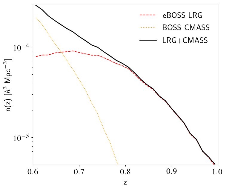
Figure 1: The observed number density of eBOSS LRGs (dashed curve), BOSS CMASS galaxies (dotted curve), and combined CMASS+LRG sample galaxies (solid curve) at $0.6<z<1$. This combines NGC and SGC fields.

2.3 Reconstruction

While constraints on the growth rate of structure are obtained using the information from the full shape of the correlation function, BAO analyses extract the cosmological information only from the position of the BAO peak. In our BAO analysis, we applied the reconstruction technique of Burden et al. (2014); Burden et al. (2015) to the observed galaxy density field in order to remove a fraction of the redshift-space distortions, as well as non-linear motions of galaxies that smeared out the BAO peak. This technique sharpens the BAO feature in the two-point statistics in Fourier and configuration space, increasing the precision of the measurement of the acoustic scale. Reconstruction is applied on actual data and on mock catalogs using a publicly available code (Bautista et al., 2018). Our final BAO results are solely based on reconstructed catalogs, while full-shape results use the pre-reconstruction sample.

We apply reconstruction to the full eBOSS+CMASS final LRG catalog. We use our fiducial cosmology from Table 1 to convert redshifts to comoving distances. For the reconstruction, we fix the bias value to $b=2.3$ and assume the standard gravity relation between the growth rate of structure and $\Omega_{m}$, i.e. $f=\Omega_{m}^{6/11}(z=0.7)=0.815$. We use a smoothing scale of $15$ $h^{-1}$Mpc. The BAO results are not sensitive to small variations of those parameter choices as studied in Carter et al. (2019).

2.4 Mocks

In order to test the overall methodology and study the impact of systematic effects, we have constructed several sets of mock samples. Approximate methods are considered to be sufficient for covariance matrix estimates and to derive systematic biases in BAO measurements. However, the full-shape analysis of the correlation function requires more realistic N-body simulations, particularly in order to test the modeling. In this study, our synthetic datasets are the following:

• 1000 realisations of the LRG eBOSS+CMASS survey geometry using the EZmock method (Chuang et al., 2015), which employs the Zel’dovich approximation to compute the density field at a given redshift and populate it with galaxies. This method is fast and has been calibrated to reproduce the two- and three-point statistics of the given galaxy sample, to a good approximation and up to mildly non-linear scales. The angular and redshift distributions of the eBOSS LRG sample in combination with the $z>0.6$ CMASS sample were reproduced in these mock catalogs. The full description of the EZmock LRG samples can be found in the companion paper Zhao et al. 2020. We use these mocks in several steps of our analysis: to infer the error covariance matrix of our clustering measurements in the data, to study the impact of observational systematic effects on cosmology, and to estimate the correlations between different methods for the calculation of the consensus results.

• 84 realisations of the Nseries mocks, which are N-body simulation snapshots populated with a single Halo Occupation distribution (HOD) model. These mock catalogs reproduce the angular and redshift distributions of the North Galactic Cap of the BOSS CMASS sample within the redshift range $0.43<z<0.70$ (Alam et al., 2017). While this dataset is not fully representative of the eBOSS LRG sample, we use these N-body mocks to test the RSD models down to the non-linear regime. The number of available realisations and their large volume are ideal to test model accuracy in the high-precision regime. The covariance matrix for these mocks were computed from 2048 realisations of the same volume with the MD-Patchy approximated method (Kitaura et al., 2014). The redshift of those mocks is $z=0.55$.

• 27 realisations extracted from the OuterRim N-body simulation (Heitmann et al., 2019), and corresponding to cubical mocks of $1~{}h^{-3}~{}{\rm Gpc}^{3}$ each. The dark matter haloes have been populated with galaxies using four different HOD (Zheng et al., 2007; Leauthaud et al., 2011; Tinker et al., 2013; Hearin et al., 2015) at 3 different luminosity thresholds to cover a large range of galaxy populations. These mocks are part of our internal MockChallenge and aimed at quantifying potential systematic errors originating from the HODs. A detailed description of these simulations and the MockChallenge can be found in the companion paper Rossi et al. (2020). The redshift of those mocks is $z=0.695$.

2.5 Fiducial cosmologies

The redshift of each galaxy is converted into radial comoving distances for clustering measurements by means of a fiducial cosmology. The fiducial cosmologies employed in this work are shown in Table 1. Our baseline choice, named “Base”, is a flat $\Lambda$CDM model matching the cosmology used in previous BOSS analyses (Alam et al., 2017) with parameters within 1$\sigma$ of Planck best-fit parameters (Collaboration et al., 2018a). Some of these cosmologies were used to produce the mock datasets described in Section 2.4. A choice of fiducial cosmology is also needed when computing the linear power spectrum $P_{\rm lin}(k)$, input for all our correlation function models in this work (see Sections 3.1 and 3.2). In Section 4.1 and Section 4.2 we study the dependence of our results to the choice of fiducial cosmology.

Table 1: Sets of cosmological models used in this work. All models are parameterised by their fraction of the total energy density in form of total matter $\Omega_{m}$, cold dark matter $\Omega_{c}$, baryons $\Omega_{b}$, and neutrinos $\Omega_{\nu}$, the Hubble constant $h=H_{0}/(100{\rm km/s/Mpc})$, the primordial spectral index $n_{s}$ and primordial amplitude of power spectrum $A_{s}$. With these parameters we compute the normalisation of the linear power spectrum $\sigma_{8}$ at $z=0$ and the comoving sound horizon scale at drag epoch $r_{\rm drag}$. The different labels refer to our baseline choice (Base), the EZmocks (EZ), the Nseries (NS), the OuterRim (OR) cosmologies, and an additional model (X) with larger value for $\Omega_{m}$.

	Base	EZ	NS	OR	$X$
$\Omega_{m}$	0.310	0.307	0.286	0.265	0.350
$\Omega_{c}$	0.260	0.259	0.239	0.220	0.300
$\Omega_{b}$	0.048	0.048	0.047	0.045	0.048
$\Omega_{\nu}$	0.0014	0	0	0	0.0014
$h$	0.676	0.678	0.700	0.710	0.676
$n_{s}$	0.970	0.961	0.960	0.963	0.970
$A_{s}$ [$10^{-9}$]	2.041	2.116	2.147	2.160	2.041
$\sigma_{8}(z=0)$	0.800	0.823	0.820	0.800	0.874
$r_{\rm drag}$ [Mpc]	147.78	147.66	147.15	149.35	143.17

Table 2: Values for the comoving angular diameter distance $D_{M}$ and the Hubble distance $D_{H}=c/H(z)$ in units of the sound horizon scale at drag epoch $r_{d}$, and the normalised growth rate of structures $f{\sigma_{8}}$. These values are predictions from the cosmological models in Table 1 computed at typical redshifts used in this work.

Model	$z_{\rm eff}$	$\frac{D_{M}}{r_{\rm drag}}$	$\frac{D_{H}}{r_{\rm drag}}$	$f{\sigma_{8}}$
Base	0.698	17.436	20.194	0.456
Base	0.560	14.529	21.960	0.465
EZ	0.698	17.429	20.211	0.467
NS	0.560	14.221	21.692	0.469
OR	0.695	16.717	19.866	0.447
X	0.698	17.685	20.146	0.504
X	0.560	14.778	22.019	0.518

We define the effective redshift of our data and mock catalogs as the weighted mean redshift of galaxy pairs,

$$z_{\rm eff}=\frac{\sum_{i>j}w_{i}w_{j}(z_{i}+z_{j})/2}{\sum_{i>j}w_{i}w_{j}},$$ (1)

where $w_{i}$ is the total weight of the galaxy $i$ and the indices $i$,$j$ run over the galaxies in the considered catalog. We only include the pairs of galaxies with separations comprised between $25$ and $130$ $h^{-1}~{}{\rm Mpc}$, which correspond to those effectively used in our full-shape analysis (see Section 3.2). By doing so, we obtain $z_{\rm eff}=0.698$ for the combined sample. The EZmocks were constructed to mimic our data sample and thus have the same $z_{\rm eff}$. The Nseries mocks were constructed to match the BOSS CMASS NGC sample and we obtain $z_{\rm eff}=0.56$. The MockChallenge mocks were produced with a snapshot at $z=0.695$ and we use this value as their effective redshift.

2.6 Galaxy clustering estimation

We estimate the redshift-space galaxy clustering in configuration space by measuring the galaxy anisotropic two-point correlation function $\xi(r,\mu)$. This measurement is performed with the standard Landy & Szalay (1993) estimator:

$$\xi(r,\mu)=\frac{GG(r,\mu)-2GR(r,\mu)+RR(r,\mu)}{RR(r,\mu)},$$ (2)

where $GG(r,\mu)$, $GR(r,\mu)$, and $RR(r,\mu)$ are respectively the normalized galaxy-galaxy, galaxy-random, and random-random number of pairs with separation $(r,\mu)$. For the post-reconstruction, we employ the same estimator except that in the numerator, displaced galaxy and random catalogs are used instead. Since we are interested in quantifying RSD effects, we decompose the three-dimensional galaxy separation vector $\vec{r}$ into polar coordinates $(r,\mu)$ aligned with the line-of-sight direction, where $r$ is the norm of the separation vector and $\mu$ is the cosine of the angle between the line-of-sight and separation vector directions. The pair counts are binned in 5$h^{-1}$Mpc bins in $r$ and 0.01 bins in $\mu$.

The measured anisotropic correlation function, where the galaxy separation vector $\vec{r}$ has been decomposed into line-of-sight and transverse separations $(r_{\perp},r_{\parallel})$, is presented in the left panel of Fig. 2. A clear BAO feature is seen at $r\approx 100$$h^{-1}$Mpc as well as the impact of RSD, which squash the contours along the line of sight on large scales. In the right panel of Fig. 2 we show the post-reconstruction correlation function where some of the isotropy is recovered and the BAO feature is sharpened.

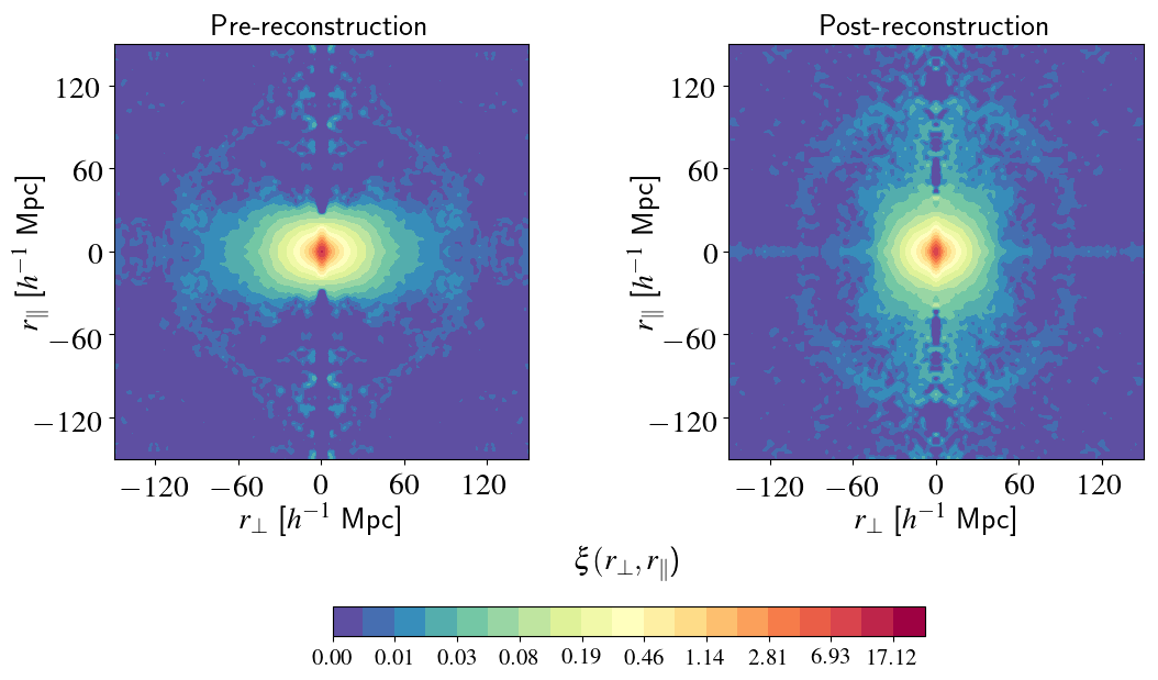
Figure 2: Anisotropic two-point correlation function of eBOSS LRG+CMASS galaxies at $0.6<z<1$. The left (right) panel shows the pre-reconstruction (post-reconstruction) two-point correlation function in bins of $r_{\perp}$ and $r_{\parallel}$. Bins of size $1.25~{}h^{-1}~{}$Mpc and a bi-cubic spline interpolation have been used to produce the contours.

For the cosmological analysis, we compress the information contained in the full anisotropic correlation function. We define the multipole moments of the correlation function by decomposing $\xi(r,\mu)$ on the basis of Legendre polynomials. Since we are working with binned data, the discrete decomposition is written as:

$$\hat{\xi}_{\ell}(r)=(2\ell+1)\sum_{i}\xi(r,\mu_{i})L_{\ell}(\mu_{i}){\rm d}\mu,$$ (3)

where only even multipoles do not vanish given the symmetry of galaxy pairs and our choice of line of sight. We note that in the previous equation there is a factor of 2 cancellation due to the imposed symmetry between negative and positive $\mu$. Throughout this work, we only consider $\ell=0$, 2 and 4 multipoles, referred to as monopole, quadrupole, and hexadecapole, respectively in the following.

The red points with error bars in Fig. 3 show the even multipoles of the correlation function from the eBOSS LRG sample. The solid, dashed, and dotted black curves display the average multipoles in the different mock datasets used in this study: EZmocks, Nseries, and MockChallenge. The error bars are obtained from the dispersion of the 1000 EZmocks multipoles around their mean. By construction, the amplitude of the EZmock multipoles matches the data at separations $s<70$$h^{-1}$Mpc. A slight mismatch in the BAO peak amplitudes between data and EZmocks is visible. This mismatch does not impact cosmological results from the data since the covariance matrix dependency on the peak amplitude is small. However, the comparison of the precision of BAO peak measurements between mocks and data needs to account for this mismatch: the expected errors of our BAO measurement are smaller for data than for the ensemble of EZmocks. For comparison, the average multipoles of the Nseries mocks, also shown in Fig. 3, are a better match to the peak amplitude seen in the data.

Pre-reconstruction

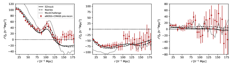
Post-reconstruction

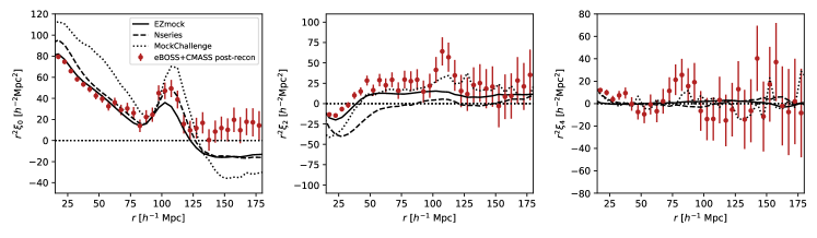
Figure 3: Multipoles of the correlation function of data compared to the mock catalogs. The data is the combined eBOSS LRG + CMASS (NGC+SGC) samples and the mocks are the average multipoles of 1000 EZmocks realisations (solid line), 84 Nseries realisations (dashed line) and 27 MockChallenge mocks populated with L11 HOD model (dotted lines). Top panels show the monopole, quadrupole and hexadecapole of the pre-reconstruction samples while bottom panels show the same for the post-reconstruction case.

3 Methodology

In this section we describe the BAO and RSD modelling, fitting procedure, and how errors on cosmological parameters are estimated.

3.1 BAO modelling

We employ the standard approach used in previous SDSS publications for measuring the baryon acoustic oscillations scale in configuration space (e.g., Anderson et al. 2014; Ross et al. 2017; Alam et al. 2017; Bautista et al. 2018). The code that produces the model and perform the fitting to the data is publicly available.

The aim is to model the correlation function multipoles $\xi_{\ell}(r)$ as a function of separations $r$ relevant for BAO ($30<r<180~{}h^{-1}$Mpc). The starting point is the model for the redshift-space anisotropic galaxy power-spectrum $P(k,\mu)$,

$$P(k,\mu)=\frac{b^{2}\left[1+\beta(1-S(k))\mu^{2}\right]^{2}}{(1+k^{2}\mu^{2}\Sigma_{s}^{2}/2)}\times\\ \times\left[P_{\rm no\ peak}(k)+P_{\rm peak}(k)e^{-k^{2}\Sigma_{\rm nl}^{2}(\mu)/2}\right]$$ (4)

where $b$ is the linear bias, $\beta=f/b$ is the redshift-space distortions parameter, $k$ is the modulus of the wave-vector and $\mu$ is the cosine of the angle between the wave-vector and the line of sight. The non-linear broadening of the BAO peak is modelled by multiplying the “peak-only” power spectrum $P_{\rm peak}$ (see below) by a Gaussian distribution with $\Sigma_{\rm nl}^{2}(\mu)=\Sigma_{\parallel}^{2}\mu^{2}+\Sigma^{2}_{\perp}(1-\mu^{2})$. The non-linear random motions on small scales are modeled by a Lorentzian distribution parametrized by $\Sigma_{s}$. When performing fits to the multipoles of a single realisation of the survey, the values of $(\Sigma_{\parallel},\Sigma_{\perp},\Sigma_{s})$ are held fixed to improve convergence. The values chosen for these damping terms were obtained from fits to the average correlation function of the Nseries mocks, which are full N-body simulations. We show in Section 4.1 that our results are insensitive to small changes to those values. Following Seo et al. (2016) theoretical considerations, we apply a term $S(k)=e^{-k^{2}\Sigma_{r}^{2}/2}$ to the post-reconstruction modeling of the correlation function ($S(k)=0$ for the pre-reconstruction BAO model). This term models the smoothing used in our reconstruction technique, where $\Sigma_{r}=15$$h^{-1}$Mpc (see Section 2.3).

We follow the procedure from Kirkby et al. (2013) to decompose the BAO peak component $P_{\rm peak}$ from the linear power-spectrum $P_{\rm lin}$. We start by computing the correlation function by Fourier transforming $P_{\rm lin}$, then we replace the correlations over the peak region by a polynomial function fitted using information outside the peak region ($50<r<80$ and $160<r<190$$h^{-1}$Mpc). The resulting correlation function is then Fourier transformed back to get $P_{\rm no\ peak}$. The linear power spectrum $P_{\rm lin}$ is computed using the code CAMB (Lewis et al., 2000) with cosmological parameters of our fiducial cosmology (Table 1). The analysis in Fourier space uses the same procedure (see Gil-Marín et al., 2020). Previous BOSS & eBOSS analyses making BAO measurements from direct tracer galaxies, used the approximate formulae from Eisenstein et al. (1998) for decomposing the peak. We have checked that both methods yield only negligibly different results.

The correlation function multipoles $\xi_{\ell}(s)$ are obtained from the multipoles of the power-spectrum $P_{\ell}(k)$, defined as:

$$P_{\ell}(k)=\frac{2\ell+1}{2}\int_{-1}^{1}P(k,\mu)L_{\ell}(\mu)~{}{\rm d}\mu$$ (5)

where $L_{\ell}$ are Legendre polynomials. The $P_{\ell}$ are then Hankel transformed to $\xi_{\ell}$ using:

$$\xi_{\ell}(r)=\frac{i^{\ell}}{2\pi^{2}}\int_{0}^{\infty}k^{2}j_{\ell}(kr)P_{\ell}(k)~{}{\rm d}k$$ (6)

where $j_{\ell}$ are the spherical Bessel functions. These transforms are computed using a Python implementation of the FFTLog algorithm described in Hamilton (2000).

We parameterise the BAO peak position in our model via two dilation parameters that scale separations into transverse, $\alpha_{\perp}$, and radial, $\alpha_{\parallel}$, directions. These quantities are related, respectively, to the comoving angular diameter distance, $D_{M}=(1+z)D_{A}(z)$, and to the Hubble distance, $D_{H}=c/H(z)$, by

$$\alpha_{\perp}=\frac{D_{M}(z_{\rm eff})/r_{d}}{D_{M}^{\rm fid}(z_{\rm eff})/r_{d}^{\rm fid}}$$ (7)

$$\alpha_{\parallel}=\frac{D_{H}(z_{\rm eff})/r_{d}}{D_{H}^{\rm fid}(z_{\rm eff})/r_{d}^{\rm fid}}$$ (8)

In our implementation, we apply the scaling factors exclusively to the peak component of the power spectrum. As shown by Kirkby et al. (2013), the decoupling between the peak and full-shape of the correlation function makes the constraints on the dilation parameters to be only dependent on the BAO peak position, with no information coming from the full-shape as it is the case for RSD analysis.

The final BAO model is a combination of the cosmological multipoles $\xi_{\ell}$ and a smooth function of separation. The smooth function is meant to account for unknown systematic effects in the survey that potentially create large-scale correlations that could contaminate our measurements. Furthermore, there are currently no accurate analytical models for the post-reconstruction multipoles to date (the $S(k)$ term in Eq. 4 is generally not sufficient). Our final template is written as:

$$\xi^{t}_{\ell}(r)=\xi_{\ell}(\alpha_{\perp},\alpha_{\parallel},r)+\sum_{i=i_{\rm min}}^{i_{\rm max}}a_{\ell,i}{r^{i}}.$$ (9)

Our baseline analysis uses $i_{\rm min}=-2$ and $i_{\rm max}=0$, corresponding to three nuisance parameters per multipole. We find that increasing the numbers of nuisance terms does not impact significantly the results. Note that this smooth function cannot be used in the full-shape RSD analysis since these terms would be completely degenerate with the growth rate of structure parameter.

Our baseline BAO analysis uses the monopole $\xi_{0}$ and the quadrupole $\xi_{2}$ of the correlation function. We performed fits on mock multipoles including the hexadecapole $\xi_{4}$, finding that it does not add information (see Table 6). We fix $\beta=0.35$ and fitting $b$ with a flat prior between $b=1.0$ and 4. For all fits, the broadband parameters are free, while both dilation parameters are allowed to vary between 0.5 and 1.5. A total of 9 parameters are fitted simultaneously.

3.2 RSD modelling

We describe the apparent distortions introduced by galaxy peculiar velocities in the redshift-space galaxy clustering pattern using two different analytical models: the combined Gaussian streaming and Convolutional Lagrangian Perturbation Theory (CLPT) formalism developed by Reid & White (2011); Carlson et al. (2013); Wang et al. (2014), and the Taruya et al. (2010) model (TNS) supplemented with a non-linear galaxy bias prescription. These two models, frequently used in the literature, partially account for RSD non-linearities and describe the anisotropic clustering down to the quasi-linear regime. We use both models to fit the multipoles of the correlation function and later combine their results to provide more robust estimates of the growth rate of structure and geometrical parameters. This procedure should reduce the residual theoretical systematic errors. In this section, we briefly describe the two models and assess in Section 4.2 their performance in the recovery of unbiased cosmological parameters using mock datasets.

3.2.1 Convolutional Lagrangian Perturbation Theory with Gaussian Streaming

CLPT provides a non-perturbative resummation of Lagrangian perturbation to the two-point statistic in configuration space for biased tracers. The Lagrangian coordinates $\vec{q}$ of a given tracer are related to their Eulerian coordinates $\vec{x}$ through the following equation:

$$\vec{x}(\vec{q},t)=\vec{q}+\vec{\Psi}(\vec{q},t),$$ (10)

where $\Psi(\vec{q},t)$ refers to the displacement field evaluated at the Lagrangian position at each time $t$. The two-point correlation function is expanded in its Lagrangian coordinates considering the tracer $X$, in our case the LRG, to be locally biased with respect to the matter overdensity $\delta(\vec{q})$. The expansion is performed over different orders of the Lagrangian bias function $F[\delta(\vec{q})]$, defined as:

$$1+\delta_{X}(\vec{q},t)=F[\delta(\vec{q})].$$ (11)

The Eulerian density contrast field is computed by convolving with the displacement:

$$1+\delta_{X}(\vec{x})=\int d^{3}q\,F\left[\delta(\vec{q})\right]\int\frac{d^{3}k}{(2\pi)^{3}}e^{i\vec{k}(\vec{x}-\vec{q}-\vec{\psi}(\vec{q}))}.$$ (12)

The local Lagrangian bias function $F$ is approximated by a non-local expansion using its first and second derivative, where the $n^{th}$ derivative is given by:

$$\langle F^{n}\rangle=\int\frac{d\delta}{\sqrt{2\pi}\sigma}e^{-\delta^{2}/2\sigma^{2}}\frac{d^{n}F}{d\delta^{n}}.$$ (13)

The two-point correlation function is obtained by evaluating the expression $\xi_{X}(\vec{r})=\left<\delta_{X}(\vec{x})\delta_{X}(\vec{x}+\vec{r})\right>$, corresponding to Eq 19 of Carlson et al. (2013), and that can be simplified as in their Eq. 46:

$$1+\xi_{X}(\vec{r})=\int d^{3}qM(\vec{r},\vec{q}),$$ (14)

where $M(\vec{r},\vec{q})$ is the kernel of convolution taking into account the displacement and bias expansion up to its second derivative term. The bias derivative terms are computed using the linear power spectrum derived from the code CAMB (Lewis et al., 2000) using the fiducial cosmology described in Table 1.

As we are interested in studying RSD, we need to model the impact of peculiar velocity. The CLPT provides the pairwise mean velocity $v_{12}(r)$ and the pairwise velocity dispersion $\sigma_{12}(r)$ as a function of the real-space separation. They are computed following the formalism developed in Wang et al. (2014), which is similar to the one describe above but modifying the kernel to take into account the velocity rather than the density:

$$v_{12}(r)=(1+\xi(\vec{r}))^{-1}\int{M_{1}}(\vec{r},\vec{q})d^{3}q,$$ (15)

and

$$\sigma_{12}(r)=(1+\xi(\vec{r}))^{-1}\int M_{2}(\vec{r},\vec{q})d^{3}q.$$ (16)

The kernels $M_{1,2}(\vec{r},\vec{q})$ also depend on the first two non-local derivatives of the Lagrangian bias $\langle F^{\prime}\rangle$ and $\langle F^{\prime\prime}\rangle$, which are free parameters in addition to the linear growth rate $f$ in our model. Hereafter, we eliminate the angle brackets around the Lagrangian bias terms to simplify the notation in the following sections.

Although CLPT is more accurate than Lagrangian Resummation Theory from Matsubara (2008) in real space, we still have to improve the small-scale modelling in order to study redshift-space distortions. This is particularly important considering that part of peculiar velocities are generated by interactions that occur at the typical scales of clusters of galaxies ($\sim$1 Mpc). This is achieved by mapping the real-space CLPT model of the two-point statistics into redshift space with the Gaussian Streaming (GS) model proposed by Reid & White (2011). The pairwise velocity distribution of tracers is assumed to have a Gaussian distribution that depends on both the separation $r$ and the angle between the separation vector and the line of sight $\mu$.

We use the Wang et al. (2014) implementation that uses CLPT results as input for the GS model. The redshift-space correlation function is finally computed as:

$$\begin{split}1+\xi_{\rm X}(r_{\perp},r_{\parallel})=&\int\frac{1}{\sqrt{2\pi\left[\sigma_{12}^{2}(r)+\sigma^{2}_{\rm FoG}\right]}}[1+\xi_{\rm X}(r)]\\ &\times\exp{-\frac{[r_{\parallel}-y-\mu v_{12}(r)]^{2}}{2\left[\sigma_{12}^{2}(r)+\sigma^{2}_{\rm FoG}\right]}}dy,\end{split}$$ (17)

where $\xi(r)$, $v_{12}(r)$, and $\sigma_{12}(r)$ are obtained from CLPT. The last function in the integral takes into account the scale-dependent halo-halo pairwise velocity and we have to introduce an extra parameter $\sigma_{\rm FoG}$ describing the galaxy random motions with respect to their parent halo, also known as Fingers-of-God (FoG) effect. Reid & White (2011) demonstrated that the GS model can predict clustering with an accuracy of $\approx 2$ per cent when dark-matter halos are used as tracers. Using galaxies, the accuracy decreases as $\sigma_{\rm FoG}$ increases. Considering that about 85 per cent of the galaxies from the LRG sample are central galaxies (Zhai et al., 2017a), the accuracy remains close to the one obtained using halos. In summary, given a fiducial cosmology, this RSD model has four free parameters $[f,F^{\prime},F^{\prime\prime},\sigma_{\rm FoG}]$.

3.2.2 TNS model

The other RSD model that we consider is the Taruya et al. (2010) model extended to non-linearly biased tracers. We refer to it as TNS in this work. Its implementation closely follows the one presented in de la Torre et al. (2017). This model is based on the conservation of the number density in real- and redshift-space (Kaiser, 1987). In this framework, the anisotropic power spectrum for unbiased matter tracers follows the general form (Scoccimarro et al., 1999)

$$P^{s}(k,\mu) = \int\frac{d^{3}\vec{r}}{(2\pi)^{3}}e^{-i\vec{k}\cdot\vec{r}}\left<e^{-ikf\mu\Delta u_{\parallel}}\times\right.$$ (18)

$$\left.[\delta(\vec{x})+f\partial_{{}_{\parallel}}u_{{}_{\parallel}}(\vec{x})][\delta(\vec{x}^{\prime})+f\partial_{{}_{\parallel}}u_{{}_{\parallel}}(\vec{x}^{\prime})]\right>$$

where $\mu=k_{\parallel}/k$, $u_{\parallel}(\vec{r})=-v_{\parallel}(\vec{r})/(faH(a))$, $v_{\parallel}(\vec{r})$ is the line-of-sight component of the peculiar velocity, $\delta$ is the matter density field, $\Delta u_{\parallel}=u_{\parallel}(\vec{x})-u_{\parallel}(\vec{x}^{\prime})$ and $\vec{r}=\vec{x}-\vec{x}^{\prime}$. The model by Taruya et al. (2010) for Eq. 18 can be written

$$P^{s}(k,\mu)=D(k\mu\sigma_{v})\big{[}P_{\delta\delta}(k)+2\mu^{2}fP_{\delta\theta}(k)+\mu^{4}f^{2}P_{\theta\theta}(k)+\\ C_{A}(k,\mu,f)+C_{B}(k,\mu,f)\big{]}\,,$$ (19)

where $\theta$ is the divergence of the velocity field defined as $\theta=-\nabla{\bf\cdot v}/(aHf)$. $P_{\delta\delta}$, $P_{\theta\theta}$ and $P_{\delta\theta}$ are respectively the non-linear matter density, velocity divergence, and density-velocity divergence power-spectra. $C_{A}(k,\mu,f)$ and $C_{B}(k,\mu,f)$ are two correction terms that reduce to integrals of the matter power spectrum given in Taruya et al. (2010). The phenomenological damping function $D(k\mu\sigma_{v})$, not only describes the FoG effect induced by random motions in virialized systems, but has also a damping effect on the power spectra. Several functional forms can be used, in particular Gaussian or Lorentzian forms have been extensively used in previous analyses. We opt for a Lorentzian damping function that provides a better agreement to the LRG data and mocks,

$$D(k,\mu,\sigma_{v})=(1+k^{2}\mu^{2}\sigma_{v}^{2})^{-1},$$ (20)

where $\sigma_{v}$ represents an effective pairwise velocity dispersion that is later treated as a nuisance parameter in the cosmological inference. This model can be generalized to the case of biased tracers by including a galaxy biasing model. In that case, the anisotropic galaxy power spectrum can be rewritten as

$$P^{s}_{\rm g}(k,\mu)=D(k\mu\sigma_{v})\big{[}P_{\rm gg}(k)+2\mu^{2}fP_{\rm{g}\theta}+\mu^{4}f^{2}P_{\theta\theta}(k)+\\ C_{A}(k,\mu,f,b_{1})+C_{B}(k,\mu,f,b_{1})\big{]}$$ (21)

where $b_{1}$ is the galaxy linear bias. The explicit expressions for $C_{A}(k,\mu,f,b_{1})$ and $C_{B}(k,\mu,f,b_{1})$ are given in, e.g., de la Torre & Guzzo (2012). We adopt here a non-linear, non-local, prescription for galaxy biasing that follows the work of McDonald & Roy (2009); Chan et al. (2012). Specifically we use renormalized pertubative bias scheme presented in Assassi et al. (2014) at 1-loop. In that case, the relation between the galaxy overdensity $\delta_{\mathrm{g}}$ and matter overdensity $\delta$ is written as

$$\delta_{\mathrm{g}}=b_{1}\delta+\frac{b_{2}}{2}\delta^{2}+b_{\mathcal{G}_{2}}\mathcal{G}_{2}+b_{\Gamma_{3}}\Gamma_{3}$$ (22)

where the two operators $\mathcal{G}_{2}$ and $\Gamma_{3}$ are defined as

$$\mathcal{G}_{2}(\phi) \equiv(\partial_{i}\partial_{j}\phi)^{2}-(\partial^{2}\phi)^{2},$$ (23)

$$\Gamma_{3}(\phi,\phi_{v}) \equiv\mathcal{G}_{2}(\phi)-\mathcal{G}_{2}(\phi_{v}),$$ (24)

and $\phi$ and $\phi_{v}$ correspond to the gravitational and velocity potentials respectively. In the local Lagrangian picture, the non-local bias parameters $b_{\mathcal{G}_{2}}$ and $b_{\Gamma_{3}}$ are related to the linear bias parameter $b_{1}$ as

$$b_{\mathcal{G}_{2}} =-\frac{2}{7}(b_{1}-1)$$ (25)

$$b_{\Gamma_{3}} =\frac{11}{42}(b_{1}-1).$$ (26)

Bispectrum analyses in halo simulations show that those relations are reasonable approximations (Chan et al., 2012; Saito et al., 2014). However, as pointed out in Sánchez et al. (2017), fixing $b_{\Gamma_{3}}$ to the local Lagrangian prediction is not necessary optimal because $b_{\Gamma_{3}}$ partially absorbs the scale dependence in $b_{1}$, which should in principle be present in the bias expansion. Moreover, local Lagrangian relation remains an approximation in the nonlinear regime (e.g. Matsubara, 2011). We investigate in Section 4 whether fixing $b_{\Gamma_{3}}$ or not is optimal for the specific case of LRG using Nseries mocks. With this biasing model, the galaxy-galaxy and galaxy-velocity divergence power spectra read (Assassi et al., 2017; Simonović et al., 2018)

$$P_{gg}(k) = b_{1}^{2}P_{\delta\delta}(k)+b_{2}b_{1}I_{\delta^{2}}(k)+2b_{1}b_{\mathcal{G}_{2}}I_{{\mathcal{G}_{2}}}(k)$$ (27)

$$+2\left(b_{1}b_{\mathcal{G}_{2}}+\frac{2}{5}b_{1}b_{\Gamma_{3}}\right)F_{\mathcal{G}_{2}}(k)+\frac{1}{4}b_{2}^{2}I_{\delta^{2}\delta^{2}}(k)$$

$$+b_{\mathcal{G}_{2}}^{2}I_{\mathcal{G}_{2}\mathcal{G}_{2}}(k)\frac{1}{2}b_{2}b_{\mathcal{G}_{2}}I_{\delta_{2}\mathcal{G}_{2}}(k)$$

$$P_{g\theta}(k) = b_{1}P_{\delta\theta}(k)+\frac{b_{2}}{4}I_{\delta^{2}\theta}(k)+b_{\mathcal{G}_{2}}I_{{\mathcal{G}_{2}}\theta}(k)$$ (28)

$$+\left(b_{\mathcal{G}_{2}}+\frac{2}{5}b_{\Gamma_{3}}\right)F_{\mathcal{G}_{2}\theta}(k).$$

In the above equations, $I_{\delta^{2}}(k)$, $I_{{\mathcal{G}_{2}}}(k)$, ${F_{\mathcal{G}_{2}}(k)}$, $I_{\delta^{2}\delta^{2}}(k)$, $I_{\mathcal{G}_{2}\mathcal{G}_{2}}(k)$, $I_{\delta_{2}\mathcal{G}_{2}}(k)$, are 1-loop integrals which expressions can be found in Simonović et al. (2018). The expressions for $I_{\delta^{2}\theta}(k)$, $I_{{\mathcal{G}_{2}}\theta}(k)$, and $F_{\mathcal{G}_{2}\theta}(k)$ integrals are nearly identical as for $I_{\delta^{2}}(k)$, $I_{{\mathcal{G}_{2}}}(k)$, and ${F_{\mathcal{G}_{2}}(k)}$, except that the $G_{2}$ kernel replaces the $F_{2}$ kernel in $I_{\delta^{2}}(k)$, $I_{{\mathcal{G}_{2}}}(k)$ and ${F_{\mathcal{G}_{2}}(k)}$. Those 1-loop integrals are computed using the method described in Simonović et al. (2018), which uses a power-law decomposition of the input linear power spectrum to perform the integrals. This allows a fast and robust computation of those integrals.

The input linear power spectrum $P_{\rm lin}$ is obtained with CAMB, while the non-linear power spectrum $P_{\delta\delta}$ is calculed from the RESPRESSO code (Nishimichi et al., 2017). This non-linear power spectrum prediction does agree very well with successful perturbation theory-based predictions such as RegPT, but extend their validity to $k\simeq 0.4$ (Nishimichi et al., 2017). This is very relevant for configuration space analysis, where one needs to have both a correct BAO amplitude and a non-vanishing signal at high $k$ to avoid aliasing in the transformation from Fourier to configuration space.

To obtain $P_{\theta\theta}$ and $P_{\delta\theta}$ power spectra, we use the universal fitting functions obtained by Bel et al. (2019) and that depend on $\sigma_{8}(z)$, $P_{\delta\delta}$, and $P_{\rm lin}$ as

$$P_{\theta\theta}(k) =P_{L}(k)e^{-k\left(a_{1}+a_{2}k+a_{3}k^{2}\right)},$$ (29)

$$P_{\delta\theta}(k) =\left(P_{\delta\delta}(k)P_{\rm lin}(k)\right)^{\frac{1}{2}}e^{-\frac{k}{k_{\delta}}-bk^{6}}.$$

The overall degree of nonlinear evolution is encoded by the amplitude of the matter fluctuation at the considered effective redshift. The explicit dependence of the fitting function coefficients on $\sigma_{8}$ is given by

$$a_{1} =-0.817+3.198\sigma_{8}$$ (30)

$$a_{2} =0.877-4.191\sigma_{8}$$

$$a_{3} =-1.199+4.629\sigma_{8}$$

$$1/k_{\delta} =-0.017+1.496\sigma_{8}^{2}$$

$$b =0.091+0.702\sigma_{8}^{2}.$$

In total, this model has either four or five free parameters, $[f,b_{1},b_{2},\sigma_{v}]$ or $[f,b_{1},b_{2},b_{\Gamma_{3}}\sigma_{v}]$, depending on the number of bias parameters that are let free. Finally, the multipole moments of the anisotropic correlation function are obtained by performing the Hankel transform of the model $P_{\ell}^{s}(k)$.

3.2.3 Alcock-Paczynski effect

For both RSD models, the Alcock & Paczynski (1979) effect implementation follows that of Xu et al. (2013). The Alcock-Paczynski distortions are simplified if we define the $\alpha$ and $\epsilon$ parameters, which characterize respectively the isotropic and anisotropic distortion components. These are related to $\alpha_{\perp}$ and $\alpha_{\parallel}$ (Eqs. 7 and 8) as

$$\alpha = \alpha_{\parallel}^{1/3}\alpha^{2/3}_{\perp}$$ (31)

$$\epsilon = \left(\alpha_{\parallel}/\alpha_{\perp}\right)^{1/3}-1,$$ (32)

For model $\xi_{0}$, $\xi_{2}$, and $\xi_{4}$, the same quantities in the fiducial cosmology are given by (Xu et al., 2013):

$$\xi^{\rm fid}_{0}(r^{\rm fid}) = \xi_{0}(\alpha r)+\frac{2}{5}\epsilon\left[3\xi_{2}(\alpha r)+\frac{d\xi_{2}(\alpha r)}{d\ln(r)}\right]$$ (33)

$$\xi^{\rm fid}_{2}(r^{\rm fid}) = \bigg{(}1+\frac{6}{7}\epsilon\bigg{)}\xi_{2}(\alpha r)+2\epsilon\frac{d\xi_{0}(\alpha r)}{d\ln(r)}+\frac{4}{7}\epsilon\frac{d\xi_{2}(\alpha r)}{d\ln(r)}$$ (34)

$$+\frac{4}{7}\epsilon\bigg{[}5\xi_{4}(\alpha r)+\frac{d\xi_{4}(\alpha r)}{d\ln(r)}\bigg{]}.$$

$$\xi^{\rm fid}_{4}(r^{\rm fid}) = \xi_{4}(\alpha r)+\frac{36}{35}\epsilon\bigg{[}-2\xi_{2}(\alpha r)+\frac{d\xi_{2}(\alpha r)}{d\ln(r)}\bigg{]}$$ (35)

$$+\frac{20}{77}\epsilon\bigg{[}3\xi_{4}(\alpha r)+2\frac{d\xi_{4}(\alpha r)}{d\ln(r)}\bigg{]}$$

$$+\frac{90}{143}\bigg{[}7\xi_{6}(\alpha r)+\frac{d\xi_{6}(\alpha r)}{d\ln(r)}\bigg{]}.$$

We note that this is an approximation for small variations around $\alpha=1$ and $\epsilon=0$ (Xu et al., 2013). Nonetheless, for the observed values on those parameters and when comparing to the model prediction based on the exact transformation, the results are virtually the same.

3.2.4 The fiducial scale at which $\sigma_{8}$ is measured

We perform an additional step in order to reduce the dependency of our $f{\sigma_{8}}$ constraints on the choice of fiducial cosmology. When fitting the correlation function multipoles, $\sigma_{8}$ is kept fixed to its fiducial value defined as

$$\sigma_{R}^{2}=\int_{0}^{\infty}{\rm d}k\ k^{2}P_{\rm lin}(k)W_{\rm TH}^{2}(Rk),$$ (36)

where $P_{\rm lin}$ is the linear matter power-spectrum predicted by the fiducial cosmology, $W_{\rm TH}$ is the Fourier transform of a top-hat function with characteristic radius of $R=8$$h^{-1}$Mpc. The resulting $f$ is scaled by $\sigma_{8}$. However, in Section 4.2 we show that the recovered $f\sigma_{8}$ has a strong dependence on the fiducial cosmology when we have best-fit $\alpha$ not close to unity. We can reduce this dependency by recomputing $\sigma_{8}$ using $R=8\alpha$$h^{-1}$Mpc, where $\alpha$ is the isotropic dilation factor (Eq. 32) obtained in the fit. In effect, this keeps the scale at which $\sigma_{8}$ is fitted fixed relative to the data in units of $h^{-1}$Mpc, which only depends on $\Omega_{m}^{\rm fid}$. This is an alternative approach to the recently proposed $\sigma_{12}$ parametrisation (Sanchez, 2020), where the radius of the top-hat function is set to $R=12$ Mpc instead of $R=8$$h^{-1}$Mpc. Unless otherwise stated, all the reported values of $f{\sigma_{8}}$ in this work provide $f{\sigma_{8}}$ where the scale is fixed in this way.

3.3 Parameter inference

The cosmological parameter inference is performed by means of the likelihood analysis of the data. The likelihood $\mathcal{L}$ is defined such that

$$-2\ln\mathcal{L}(\theta)=\sum_{i,j}^{N_{p}}\Delta_{i}(\theta)\hat{\Psi}_{ij}\Delta_{j}(\theta),$$ (37)

where $\theta$ is the vector of parameters, $\vec{\Delta}$ is the data-model difference vector, $N_{p}$ is the total number of data points. An estimate of the precision matrix $\hat{\Psi}=(1-D)\hat{C}^{-1}$ is obtained from the covariance $\hat{C}$ from 1000 realisation of EZmocks, where $D=(N_{p}+1)/(N_{\rm mocks}-1)$ is a factor that accounts for the skewed nature of the Wishart distribution (Hartlap et al., 2007). The data vector that enters in $\vec{\Delta}$ includes, in the baseline configuration, the monopole and quadrupole correlation functions for the BAO analysis, and the monopole, quadrupole, and hexadecapole correlation functions for the RSD analysis.

In the BAO analysis, the best-fit parameters ($\alpha_{\perp},\alpha_{\parallel}$) are found by minimizing $-2\ln\mathcal{L}=\chi^{2}$ using a quasi-Newton minimum finder algorithm iMinuit. The errors in $\alpha_{\parallel}$ and $\alpha_{\perp}$ are found by computing the intervals where $\chi^{2}$ increases by unity. Gaussianity is not assumed in the error calculation, but we find that on average, errors are symmetric and correctly described by a Gaussian. The 2D errors in $(\alpha_{\perp},\alpha_{\parallel})$, such as those presented in Figure 13, are found by scanning $\chi^{2}$ values in a regular grid in $\alpha_{\perp}$ and $\alpha_{\parallel}$. In the case of the full-shape analysis, we explore the likelihood with the Markov chain Monte Carlo ensemble sampler emcee. The input power spectrum shape parameters are fixed at the fiducial cosmology and any deviations are accounted for through the Alcock-Paczynski parameters $\alpha_{\perp}$ and $\alpha_{\parallel}$. We assume the uniform priors on model parameters given in Table 3.

Table 3: List of fitter parameters and their priors used in full-shape analysis for the two models.

Par. TNS	Prior TNS	Par. CLPT-GS	Prior CLPT-GS
$\alpha_{\perp}$	$[0.5,1.5]$	$\alpha_{\perp}$	$[0.5,1.5]$
$\alpha_{\parallel}$	$[0.5,1.5]$	$\alpha_{\parallel}$	$[0.5,1.5]$
$f$	$[0,2]$	$f$	$[0,2]$
$b_{1}$	$[0.2,4]$	$\langle F^{\prime}\rangle$	[0,3]
$b_{2}$	$[-10,10]$	$\langle F^{\prime\prime}\rangle$	[-10,10]
$b_{\Gamma_{3}}$	$[-2,4]$	$\sigma_{\rm FoG}$	[0,40]
$\sigma_{v}$	$[0.1,8]$

Table 4: Characteristics of the baseline fits for all models in this work, where $N_{\rm mock}$ is the number of mocks used in the estimation of the covariance matrix, $N_{\rm par}$ is the total number of parameters fitted, $N_{\rm bins}$ is the total size of the data vector, $(1-D)$ is the correction factor to the precision matrix (Hartlap et al., 2007), $m_{1}$ is the factor to be applied to the estimated error matrix and $m_{2}$ is the factor that scales the scatter of best-fit parameters of a set of mocks (if these were used in the calculation of the covariance matrix). The derivation of $m_{1}$ and $m_{2}$ can be found in Percival et al. (2014).

	BAO	RSD TNS	RSD CLPT-GS
$N_{\rm mock}$	1000	1000	1000
$N_{\rm par}$	9	7	6
$N_{\rm bins}$	40	65	63
$(1-D)$	0.96	0.93	0.94
$m_{1}$	1.022	1.053	1.053
$m_{2}$	1.065	1.128	1.125

The final parameter constraints are obtained by marginalizing the full posterior likelihood over the nuisance parameters. The marginal posterior is approximated by a multivariate Gaussian distribution with central values given by best-fitting parameter values $\theta^{*}=(\alpha_{\perp},\alpha_{\parallel},f{\sigma_{8}})$ and parameter covariance matrix $C_{\theta}$. Since the covariance matrix is computed from a finite number of mock realisations, we need to apply correction factors to the obtained $C_{\theta}$. These factors are Eq. 18 and 22 from Percival et al. (2014) to be applied to uncertainties and to the scatter over best-fit values, respectively. These factors, which depend on the number of mocks, parameters and bins in the data vectors, are presented in Table 4. The final parameter constraints from this work are available to the public in this format.

3.4 Combining BAO and RSD constraints

From the same input LRG catalog, we produced BAO-only and full-shape RSD constraints, both in configuration and Fourier space (Gil-Marín et al., 2020). Each measurement yields a marginal posterior on $(\alpha_{\perp},\alpha_{\parallel})$ for BAO-only or $(\alpha_{\perp},\alpha_{\parallel},f{\sigma_{8}})$ for the full-shape RSD analyses. In the following we describe the procedure to combine all these posteriors into a single consensus constraint, while correctly accounting for their covariances. This consensus result is the one used for the final cosmological constraints described in eBOSS collaboration (2020).

We follow closely the method presented in Sánchez et al. (2017) to derive the consensus result. The idea is to compress $M$ data vectors $x_{m}$ containing $p$ parameters and their $p\times p$ covariance matrices $C_{mm}$ from different methods into a single vector $x_{c}$ and covariance $C_{c}$, assuming that the $\chi^{2}$ between individual measurements is the same as the one from the compressed result. The expression for the combined covariance matrix is

$$C_{c}\equiv\left(\sum_{m=1}^{M}\sum_{n=1}^{M}C_{mn}^{-1}\right)^{-1}$$ (38)

and the combined data vector is

$$x_{c}=C_{c}\sum_{m=1}^{M}\left(\sum_{n=1}^{M}C^{-1}_{nm}\right)x_{m}$$ (39)

where $C_{mn}$ is a $p\times p$ block from the full covariance matrix between all parameters and methods $C$, defined as

$$C=\begin{pmatrix}C_{11}&C_{12}&\cdots&C_{1M}\\ C_{21}&C_{22}&\cdots&C_{2M}\\ \vdots&\vdots&\ddots&\vdots\\ C_{M1}&C_{M2}&\cdots&C_{MM}\end{pmatrix}$$ (40)

The diagonal blocks $C_{mm}$ are obtained from the Gaussian approximation of the marginal posterior from each method. The off-diagonal blocks $C_{mn}$ with $m\neq n$ cannot be estimated from our fits. We derive these off-diagonal blocks from results from each method applied to the 1000 EZmocks realisations. More precisely, we compute the correlation coefficients $\rho^{\rm mocks}_{p_{1},p_{2},m,n}$ between parameters $p_{1}$, $p_{2}$ and methods $m,n$ using the mocks and scale these coefficients by the diagonal errors from the data. It is worth emphasizing that the correlation coefficients between parameters depend on the given realisation of the data, while the ones derived from mock measurements are ensemble averaged coefficients. Therefore, we scale the correlations coefficients from the mocks in order to match the maximum correlation coefficient that would be possible with the data (Ross et al., 2015b). For the same parameter $p_{1}$ measured by two different methods $m$ and $n$, we assume that the maximum correlation between them is given by $\rho_{\rm max}=\sigma_{p1,m}/\sigma_{p1,n}$, where $\sigma_{p}$ is the error of parameter $p$. This number is computed for the data realisation $\rho_{\rm max}^{\rm data}$ and for the ensemble of mocks $\rho_{\rm max}^{\rm mocks}$. We can write the adjusted correlation coefficients as

$$\rho^{\rm data}_{p_{1},p_{1},m,n}=\rho^{\rm mocks}_{p_{1},p_{1},m,n}\frac{\rho^{\rm data}_{\rm max}}{\rho^{\rm mocks}_{\rm max}}$$ (41)

The equation above accounts for the diagonal terms of the off-diagonal block $C_{mn}$. For the off-diagonal terms, we use

$$\rho^{\rm data}_{p_{1},p_{2},m,n}=\frac{1}{4}\left(\rho^{\rm data}_{p_{1},p_{1},m,n}+\rho^{\rm data}_{p_{2},p_{2},m,n}\right)\left(\rho^{\rm data}_{p_{1},p_{2},m,m}+\rho^{\rm data}_{p_{1},p_{2},n,n}\right)$$ (42)

We use the method described above to perform all the constraint combinations, except for the combination of results from CLPT-GS and TNS RSD models, which use the same input data vector (pre-reconstruction multipoles in configuration space). For this particular combination, we simply assume that $C_{c}^{-1}=0.5(C_{mm}^{-1}+C_{nn}^{-1})$ and $x_{c}=2C_{c}^{-1}\left(C_{mm}^{-1}x_{m}+C_{nn}^{-1}x_{n}\right)$. For all combinations, we chose to use the results from at most two methods at once ($M=2$) in order to reduce the potential noise introduced by the procedure.

Denoting $\xi_{\ell}$ the results from the configuration space analysis and $P_{\ell}$ that from the Fourier space analysis, our recipe to obtain the consensus result for the LRG sample is as follows:

• Combine RSD $\xi_{\ell}$ TNS and RSD $\xi_{\ell}$ CLPT-GS results into RSD $\xi_{\ell}$,

• Combine BAO $\xi_{\ell}$ with BAO $P_{\ell}$ into BAO $(\xi_{\ell}+P_{\ell})$,

• Combine RSD $\xi_{\ell}$ with RSD $P_{\ell}$ into RSD $(\xi_{\ell}+P_{\ell})$,

• Combine BAO $(\xi_{\ell}+P_{\ell})$ with RSD $(\xi_{\ell}+P_{\ell})$ into BAO$+$RSD $(\xi_{\ell}+P_{\ell})$

Alternatively, we can proceed as

• Combine BAO $\xi_{\ell}$ with RSD $\xi_{\ell}$ into (BAO$+$RSD) $\xi_{\ell}$,

• Combine BAO $P_{\ell}$ with RSD $P_{\ell}$ into (BAO$+$RSD) $P_{\ell}$

• Combine BAO$+$RSD $\xi_{\ell}$ with BAO$+$RSD $P_{\ell}$ into (BAO$+$RSD) $\xi_{\ell}+P_{\ell}$

In Section 4.3 we test this procedure on the mock catalogues.

4 Robustness of the analysis and systematic errors

In this section we perform a comprehensive set of tests of the adopted methodology using all the simulated datasets available. We estimate the biases in the measurement of the cosmological parameters ($\alpha_{\perp},\alpha_{\parallel},f{\sigma_{8}}$) and derive the systematic errors for both BAO-only and full-shape RSD analyses. For a given parameter, we define the systematic error $\sigma_{p,\rm syst}$ as follows. We compare the estimated value of the parameter $x_{p}$ to a reference value $x_{p}^{\rm ref}$ and set the systematic error value to

$$\sigma_{p,\rm syst}=2\sigma_{p},\ {\rm if}\ |x_{p}-x_{p}^{\rm ref}|<2\sigma_{p},$$ (43)

$$\sigma_{p,\rm syst}=|x_{p}-x_{p}^{\rm ref}|,\ {\rm if}\ |x_{p}-x_{p}^{\rm ref}|>2\sigma_{p},$$ (44)

where $\sigma_{p}$ is the estimated statistical error on $x_{p}$. As a conservative approach, we use the maximum value of the bias amongst the several cases studied.

4.1 Systematics in the BAO analysis

The methodology described in Section 3.1 was tested using the 1000 EZmocks mock survey realisations and 84 Nseries realisations. For each realisation, we compute the correlation function and its multipoles, and fit for the BAO peak position to determine the dilation parameters $\alpha_{\parallel}$, $\alpha_{\perp}$ and associated errors. We compare the best-fit $\alpha_{\perp},\alpha_{\parallel}$ to their expected values, which are obtained from the cosmological models described in Table 1. The effective redshift of the EZmocks is $z_{\rm eff}=0.698$ and $z_{\rm eff}=0.56$ for Nseries.

In Figure 4 we summarize the systematic biases from pre- and post-reconstruction mocks for a few choices of fiducial cosmology, parameterised by $\Omega_{m}^{\rm fid}$. In pre-reconstruction mocks, biases in the recovered $\alpha$ values reach up to 0.5 per cent in $\alpha_{\perp}$ and 1.0 per cent in $\alpha_{\parallel}$. These biases are expected due to the impact of non-linear effects on the position of the peak that cannot be correctly accounted for with the Gaussian damping terms in Eq. 4 at this level of precision (Seo et al., 2016). We recall that we are fitting the average of all realisations. The reconstruction procedure removes in part the non-linear effects and this is seen as a reduction of the biases to less than 0.2 per cent. The bias reduction is also seen in the Nseries mocks, particularly on $\alpha_{\perp}$, confirming that the bias reduction is not related to a feature of the mocks induced by the approximate method used to build them.

Pre-reconstruction

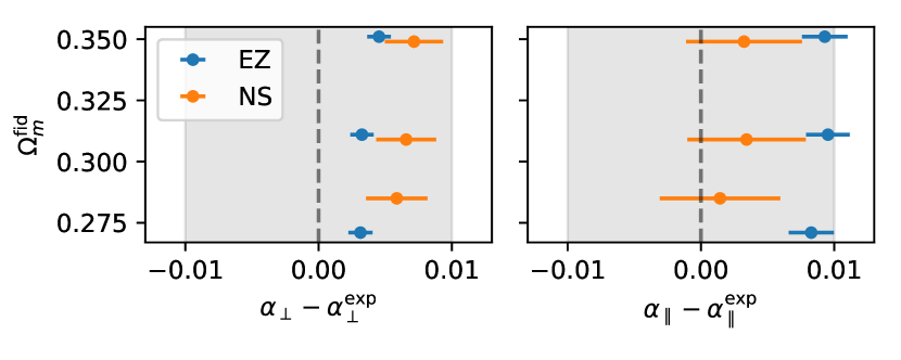
Post-reconstruction

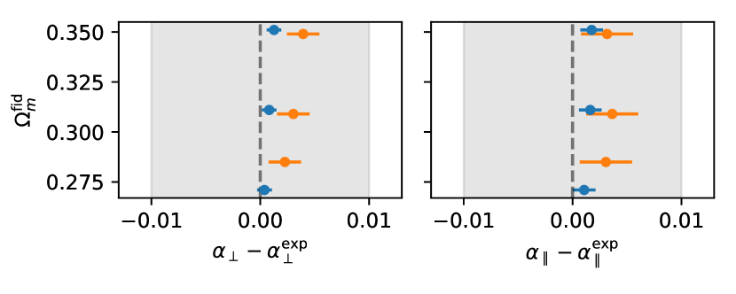
Figure 4: Impact of choice of fiducial cosmology in the recovered values of $\alpha_{\parallel}$ and $\alpha_{\perp}$ from the stacks of 1000 multipoles from the EZmocks (blue) and 84 Nseries mocks (orange), for pre- (top panels) and post- (bottom panels) reconstruction. Associated error bars correspond to the error on the mean of the mocks. The gray shaded areas correspond to one per cent errors. For comparison, the error on real data is near 1.9 per cent for $\alpha_{\perp}$ and 2.6 per cent for $\alpha_{\parallel}$ in the post-reconstruction case.

Table 5 shows results from Figure 4 for the post-reconstruction case only, including the fits with the hexadecapole $\xi_{\ell=4}$. The impact of the hexadecapole is negligible even in this very low-noise regime, for both types of mocks. The reported dilation parameters for almost all cases are consistent with expected value within 2$\sigma$. We see a 2.6$\sigma$ deviation on $\alpha_{\perp}$ for the Nseries case analysed with $\Omega_{m}^{\rm fid}=0.35$. However this choice of $\Omega_{m}^{\rm fid}$ is the most distant from the true value of the simulation and its observed bias is still less than half a per cent, which is small compared to the statistical power of our sample. For the EZmocks, which have smaller errors, the biases are up to 0.13 per cent for $\alpha_{\perp}$ and 0.18 per cent for $\alpha_{\parallel}$. These biases are much smaller than the expected statistical errors in our data, i.e. $\sim$1.9 per cent for $\alpha_{\perp}$ and $\sim$2.6 per cent for $\alpha_{\parallel}$, showing that our methodology is robust at this statistical level. In these fits, all parameters except $\Sigma_{\rm rec}=15$$h^{-1}$Mpc were left free. The best-fit values of $\Sigma_{\perp},\Sigma_{\parallel}$ and $\Sigma_{s}$ were used and held fixed in the fits of individual realisations.

Table 5: Average biases from BAO fits on the stacked multipoles of 1000 EZmocks and 84 Nseries realisations. All results are based on post-reconstruction correlation functions.

Sample	$\Omega_{m}^{\rm fid}$	$\ell_{\rm max}$	$\alpha_{\perp}-\alpha_{\perp}^{\rm exp}\ [10^{-3}]$	$\alpha_{\parallel}-\alpha_{\parallel}^{\rm exp}\ [10^{-3}]$
EZ	0.27	2	$0.4\pm 0.7$	$1.1\pm 1.0$
EZ	0.27	4	$0.5\pm 0.7$	$1.4\pm 1.0$
EZ	0.31	2	$0.9\pm 0.7$	$0.3\pm 1.1$
EZ	0.31	4	$1.0\pm 0.7$	$0.4\pm 1.1$
EZ	0.35	2	$1.3\pm 0.7$	$1.8\pm 1.0$
EZ	0.35	4	$1.2\pm 0.7$	$1.5\pm 1.0$
NS	0.286	2	$2.3\pm 1.5$	$3.1\pm 2.4$
NS	0.286	4	$2.2\pm 1.5$	$3.0\pm 2.4$
NS	0.31	2	$3.0\pm 1.5$	$3.6\pm 2.4$
NS	0.31	4	$3.0\pm 1.5$	$3.7\pm 2.4$
NS	0.35	2	$3.9\pm 1.5$	$3.2\pm 2.4$
NS	0.35	4	$3.9\pm 1.5$	$3.5\pm 2.4$

Results from Table 5 and Figure 4 show no statistically significant dependence of results with the choice of fiducial cosmology. We derived the systematic errors for the BAO analysis using the values from Table 5 and Eqs. 43 and 44. We used only the fits to the EZmocks which have the better precision. The systematic errors are for $\alpha_{\perp}$ and $\alpha_{\parallel}$, respectively:

$${\rm BAO}:\ \sigma_{\rm syst,model}=(0.0014,0.0021)$$ (45)

which are negligible compared to statistical errors of one realisation of our data. Note that the fiducial cosmologies considered are all flat and assume general relativity. Carter et al. (2019) and Bernal et al. (2020) find that BAO measurements are robust to a larger variety of fiducial cosmologies (but all close to the assumed one). Additional systematic errors should be anticipated when extrapolating to cosmologies that are significantly different than the truth, for instance yielding dilation parameters significantly different than unity.

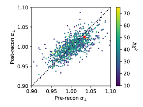
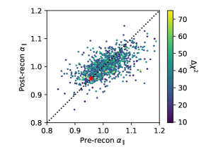
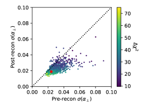
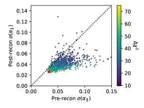
Figure 5: Distribution of dilation parameters $\alpha_{\perp}$ and $\alpha_{\parallel}$ and its estimated errors for pre and post reconstruction EZmock catalogs with systematic effects. The color scale indicates the difference in $\chi^{2}$ values between a model with and without BAO peak. The red stars shows results with real data. There is a known mismatch in the BAO peak amplitude between data and EZmocks causing the accuracy of the data point to be slightly smaller than the error distribution in the EZmocks (see Section 2.4).

Figure 5 displays the distribution of recovered $\alpha_{\perp}$, $\alpha_{\parallel}$ and their respective errors measured from each of the individual EZmocks. The error distribution shows that reconstruction improves the constraints on $\alpha_{\perp}$ or $\alpha_{\parallel}$ in 94 per cent of the realisations (89 per cent have both errors improved). As expected, realisations with smaller errors generally exhibit larger values of $\Delta\chi^{2}=\chi^{2}_{\rm no\ peak}-\chi^{2}_{\rm peak}$, meaning a more pronounced BAO peak and higher detection significance. We see no particular trend in the best-fit $\alpha$ values with $\Delta\chi^{2}$ in the two top panels. The red stars in Figure 5 indicate the values obtained in real data. The error in $\alpha_{\perp}$ in the data is typical of what is found in mocks, although for $\alpha_{\parallel}$ it is found at the extreme of the mocks distribution. As discussed in Section 2.4 and displayed in Figure 3, the BAO peak amplitude in the data multipoles is slightly larger than the one seen in this EZmock sample. A similar behaviour is observed in the eBOSS QSO sample (Hou et al., 2020; Neveux & Burtin, 2020) who also use EZmocks from Zhao et al. (2020) and in the BOSS DR12 CMASS sample (see Figure 12 of Ross et al. 2017).

Table 6 presents a statistical summary of the fits performed on the EZmocks. We tested several changes to our baseline analysis: include the hexadecapole, change the separation range $[r_{\rm min},r_{\rm max}]$, allow BAO damping parameters $\Sigma_{\perp}$ and $\Sigma_{\parallel}$ to vary within a Gaussian prior ($5.5\pm 2$$h^{-1}$Mpc), and fit the pre-reconstruction multipoles. We remove realisations with fits that did not converge or with extreme error values (more than 5$\sigma$ of their distribution, where $\sigma$ is defined as the half the range covered by 68 per cent of values). The total number of valid realisations is given by $N_{\rm good}$ in Table 6. In most cases studied, the observed standard deviation of the best-fit parameters $\sigma(\alpha)$ is consistent with the average per-mock error estimates $\langle\sigma_{\alpha}\rangle$, indicating that our errors are correctly estimated. We also see that the dispersion of dilation parameters is not significantly reduced when adding the hexadecapole $\xi_{4}$ to the BAO fits, showing that most of the BAO information is contained in the monopole and quadrupole at this level of precision. The mean and dispersion of the pull parameter, defined as $Z_{\alpha}=(\alpha-\langle\alpha\rangle)/\sigma_{\alpha}$, are consistent with an unit Gaussian for almost all cases, which further validates our error estimates.

Table 6: Statistics on errors from BAO fits on 1000 EZmocks realisations. All results are based on post-reconstruction correlation functions. $\sigma$ is the scatter of best-fit values $x_{i}$ amongst the $N_{\rm good}$ realisations with confident detection or non-extreme values or errors (out of the 1000), $\langle\sigma_{i}\rangle$ is the mean estimated error per mock, $Z=(x_{i}-\langle x_{i}\rangle)/\sigma_{i}$ is the pull quantity for which we show the mean $\langle Z_{i}\rangle$ and standard deviation $\sigma(Z)$. First row corresponds to our baseline analysis.

Analysis	$N_{\rm good}$		$\alpha_{\perp}$					$\alpha_{\parallel}$
			$\sigma$	$\langle\sigma_{i}\rangle$	$\langle Z_{i}\rangle$	$\sigma(Z_{i})$		$\sigma$	$\langle\sigma_{i}\rangle$	$\langle Z_{i}\rangle$	$\sigma(Z_{i})$
baseline	990		0.022	0.023	-0.02	$0.99$		0.035	0.036	-0.03	$0.96$
$\ell_{\rm max}=4$	995		0.022	0.023	-0.02	$0.99$		0.035	0.035	-0.03	$0.97$
pre-recon	968		0.030	0.030	-0.05	$1.07$		0.055	0.056	-0.06	$0.97$
pre-recon $\ell_{\rm max}=4$	968		0.029	0.028	-0.03	$1.04$		0.054	0.054	-0.07	$1.02$
$r_{\rm min}=20$$h^{-1}$Mpc	979		0.023	0.026	-0.01	$0.93$		0.035	0.040	0.04	$1.26$
$r_{\rm min}=30$$h^{-1}$Mpc	987		0.023	0.024	-0.02	$0.95$		0.036	0.038	-0.02	$0.92$
$r_{\rm min}=40$$h^{-1}$Mpc	995		0.022	0.023	-0.02	$0.98$		0.035	0.036	-0.02	$0.94$
$r_{\rm max}=160$$h^{-1}$Mpc	989		0.022	0.023	-0.02	$0.99$		0.036	0.036	-0.03	$0.96$
$r_{\rm max}=170$$h^{-1}$Mpc	989		0.022	0.023	-0.02	$0.99$		0.036	0.036	-0.03	$0.96$
$r_{\rm max}=180$$h^{-1}$Mpc	990		0.022	0.023	-0.02	$0.98$		0.035	0.036	-0.03	$0.95$
Prior $\Sigma_{\perp,\parallel}$	993		0.022	0.023	-0.02	$1.00$		0.035	0.035	-0.03	$0.96$

All the tests performed in this section show that our BAO analysis is unbiased and provides correct error estimates. We apply our baseline analysis to the real data and report results in Section 5.1.

4.2 Systematics in the RSD analysis

We present in this section the systematic error budget of the full-shape RSD analysis. Particularly, we discuss the impact of the choice of scales used in the fit, the bias introduced by each model, the bias introduced by varying the fiducial cosmology, the bias associated to the choice of the LRG halo occupation distribution model, and the impact of observational effects. These are quantified through the analysis of the various sets of mocks with both TNS and CLPT-GS models, which are described in Section 3.2.

4.2.1 Optimal fitting range of scales

We first study the optimal range of scales in the fit for the two RSD models considered in this work (see Section 3). It is worth noting that the optimal range of scales is not necessarily the same for the two models. Generally, full-shape RSD analyses use scales going from tens of $h^{-1}$Mpc to about $130-150\,$$h^{-1}$Mpc. Including smaller scales potentially increases the precision of the constraints but at the expense of stronger biases on the recovered parameters. This is related to the limitations of current RSD models to fully describe the non-linear regime. On the other hand, including scales larger than $\sim 130$ $h^{-1}$Mpc does not significantly improve the precision, since the variations of the model on those scales are small.

In order to determine the optimal range of scales for our RSD models, we performed fits to the mean correlation function of the Nseries mocks, which are those that most accurately predict the expected RSD in the data. Figure 6 shows the best-fit values of $f{\sigma_{8}}$, $\alpha_{\parallel}$, and $\alpha_{\perp}$ as a function of the minimum scale used in the fit, $r_{\rm min}$. In each panel, the grey bands show 1 per cent errors in $\alpha_{\perp},\alpha_{\parallel}$ and 3 per cent errors in $f{\sigma_{8}}$ for reference. Top panels present the measurements from the TNS model when the parameter $b_{\Gamma 3}$ fixed to the value given by Eq. 26, while in the mid panels this parameter is let free. Bottom panels show best-fit values for the CLPT-GS model as studied in Icaza-Lizaola et al. (2020). As noted in Zarrouk et al. (2018), the hexadecapole is more sensitive to the difference between the true and fiducial cosmologies and is generally less well modelled on small scales compared to the monopole and quadrupole. We therefore consider the possibility of having a different minimum fitting scale for the hexadecapole with respect to the monopole and quadrupole that share the same $r_{\rm min}$. For consistency with the other systematic tests, we performed this analysis using two choices of fiducial cosmologies, $\Omega^{\rm fid}_{m}=0.286$ (blue) and $\Omega^{\rm fid}_{m}=0.31$ (red). The maximum separation in all cases is $r_{\rm max}=130$$h^{-1}$Mpc, as we find that using larger $r_{\rm max}$ has a negligible impact on the recovered parameter values and associated errors.

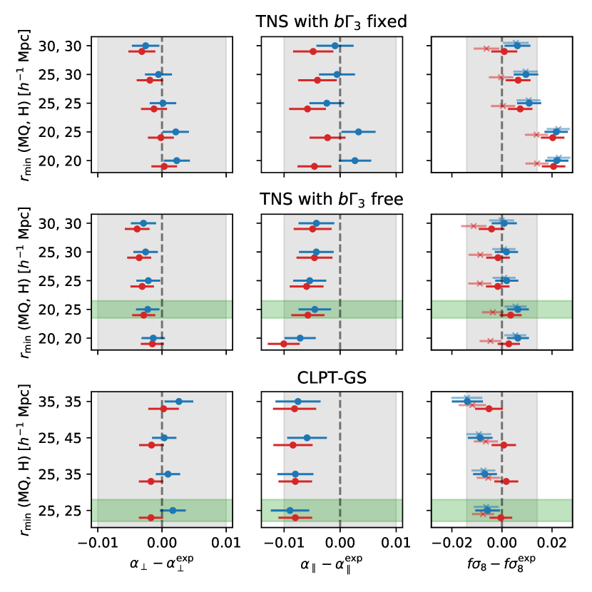
Figure 6: Biases in the measurement of $f{\sigma_{8}},\alpha_{\parallel},\alpha_{\perp}$ obtained from full-shape fits to the average of 84 multipoles from the Nseries mocks as a function of the separation range used. The y-axis displays the value of the minimal separation $r_{\rm min}$ used in fits of the monopole, quadrupole (MQ) and hexadecapole (H). Top and mid rows display results for the TNS model when fixing or letting free the parameter $b\Gamma_{3}$ respectively. Bottom row presents results for the CLPT-GS model. The blue circles correspond to the analysis using $\Omega_{m}^{\rm fid}=0.286$ (the true value of simulations) while the red squares correspond to $\Omega_{m}^{\rm fid}=0.31$. The gray shaded areas correspond to 1 per cent errors in $\alpha_{\perp},\alpha_{\parallel}$ and to 3 per cent in $f{\sigma_{8}}$. The green shared area shows our choice for baseline analysis for TNS and CLPT-GS models.

In the case of the TNS model, we consider two different cases that correspond to when $b_{\Gamma 3}$ is fixed to its Lagrangian prediction and when $b_{\Gamma 3}$ is allowed to vary. In the case of $\Omega^{\rm fid}_{m}=0.286$ and when $b_{\Gamma 3}$ is fixed, in the top panels of Figure 6, we can see that $f\sigma_{8}$ is overestimated by 1.5 per cent when using scales above 25$h^{-1}$Mpc and by 2 per cent below. Using $r_{\rm min}>25$$h^{-1}$Mpc reduces the bias to about 1 per cent on $f\sigma_{8}$. For $\alpha_{\parallel}$ and $\alpha_{\perp}$ parameters, biases range from 0.3 to 0.5 per cent and are all statistically consistent with zero. When $b_{\Gamma 3}$ is let free, in the mid panels of Figure 6, the model provide more robust measurements of $f\sigma_{8}$ at all tested ranges. The biases in $f\sigma_{8}$ over all ranges does not exceed 0.6$\sigma$, compared to approx 2.5$\sigma$ for the fixed $b_{\Gamma 3}$ case. We also remark that letting $b_{\Gamma_{3}}$ free also provides a better fit to the BAO amplitude and the hexadecapole on the scales of $20-25$$h^{-1}$Mpc. We see a 1 per cent bias on $\alpha_{\parallel}$ when $r_{\rm min}=20$$h^{-1}$Mpc for all three multipoles. This bias is however reduced by increasing the hexadecapole minimum scale to $r_{\rm min}=25$$h^{-1}$Mpc. The most optimal configuration for the TNS model is to let $b\Gamma_{3}$ free and fit the monopole and quadrupole in the range $20\leq r\leq 130$$h^{-1}$Mpc and the hexadecapole in the range $25\leq r\leq 130$$h^{-1}$Mpc, as marked by the green band in Figure 6. If we use $\Omega^{\rm fid}_{m}=0.31$, the trends and quantitative results are similar to the case with $\Omega^{\rm fid}_{m}=0.286$.

For the CLPT-GS model, an exploration of the optimal fitting range was done in Icaza-Lizaola et al. (2020). Two sets of tests have been performed. The first set consisted of fitting the mean of the mocks when varying $r_{\rm min}$ and the second, fitting the 84 individual mocks and measuring the bias and variance of the best fits when varying $r_{\rm min}$. We revisit the first set of tests, but this time performing a full MCMC analysis to determine best fits and errors. The bottom panels of Figure 6 summarise the results. In the case of $\Omega^{\rm fid}_{m}=0.286$, we see that using $r_{\rm min}=25$$h^{-1}$Mpc for all multipoles yields to biases of 0.1, 1.1 and 1.6 per cent in $\alpha_{\perp}$, $\alpha_{\parallel}$, and $f\sigma_{8}$. Increasing $r_{\rm min}$ for the hexadecapole while fixing $r_{\rm min}=25$$h^{-1}$Mpc for the monopole and quadrupole, does not change the results significantly, the biases are 0.1 per cent for all ranges in $\alpha_{\perp}$, and 1 per cent also for all ranges in $\alpha_{\parallel}$. For $f\sigma_{8}$ variations of 0.1-0.2 per cent arises when varying the range, but this variation in statistically consistent with zero. In the case of $\Omega^{\rm fid}_{m}=0.31$, we find very similar trends. Using $r_{\rm min}=25$$h^{-1}$Mpc for all multipoles yields biases of 0.2, 0.9 and 1.6 in $\alpha_{\perp}$, $\alpha_{\parallel}$ and $f\sigma_{8}$ respectively. When we decrease the range of the fits, the biases on $(\alpha_{\perp},\alpha_{\parallel},f{\sigma_{8}})$ varies by (0.1-0.2, 0.2-0.3, 0.3-0.4) per cent. These variations are not significant and we decide to keep the lowest considered minimum scales on the hexadecapole in the fits.

Compared with previous BOSS full-shape RSD analysis in configuration space, we used for CLPT-GS model the same minimum scale for the monopole and quadrupole (Satpathy et al., 2017; Alam et al., 2017). The hexadecapole was not included in BOSS analyses. The exploration for the optimal minimum scale to be used for the hexadecapole was done in Icaza-Lizaola et al. (2020) and revisited in this work. The systematic error associated to the adopted fitting range is also consistent with previous results for the case where only the monopole and quadrupole are used, as reported in Icaza-Lizaola et al. (2020). The TNS model was not used in configuration space for analysing previous SDSS samples. However, as we describe in section 4.2.2, the bias associated with both models when using their optimal fitting range is consistent between them, as well as consistent with previous BOSS results.

Overall, these tests performed on the Nseries mocks allow us to define the optimal fitting ranges of scales for both RSD models. Minimizing the bias of the models while keeping $r_{\rm min}$ as small as possible, we eventually adopt the following optimal ranges:

• TNS model: $20<r<130$$h^{-1}$Mpc for $\xi_{0}$ and $\xi_{2}$, and $25<r<130$$h^{-1}$Mpc for $\xi_{4}$

• CLPT-GS model: $25<r<130$$h^{-1}$Mpc for all multipoles,

which serve as baseline in the following. We compare the performance of the two models using these ranges in the following sections.

4.2.2 Systematic errors from RSD modeling and adopted fiducial cosmology

We quantify in this section the systematic error introduced by the RSD modelling and the choice of fiducial cosmology. For this, we used the Nseries mocks. The measurements of $\alpha_{\perp}$, $\alpha_{\parallel}$ and $f\sigma_{8}$ from fits to the average multipoles are given in Table 7 and shown in Figure 7. The shaded area in the figure corresponds to 1 per cent deviation for $\alpha_{\perp},\alpha_{\parallel}$ expected values and 3 per cent for $f{\sigma_{8}}$ expected value. We used both TNS (red) and CLPT-GS (blue) models and consider three choices of fiducial cosmologies parameterised by their value of $\Omega_{m}^{\rm fid}$. Note that, as for the BAO analysis, we only test flat $\Lambda$CDM models close to the most probable one. We expect the full-shape analysis to be biased if the fiducial cosmology is too different from the truth (the parametrisation with $\alpha_{\perp}$ and $\alpha_{\parallel}$ would not fully account for the distortions and the template power spectrum would differ significantly).

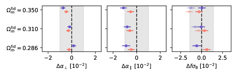
Figure 7: Biases in best-fit parameters for both CLPT-GS (blue) and TNS (red) models from fits to the average multipoles of 84 Nseries mocks. Shaded grey areas show the equivalent of 1 per cent error for $\alpha_{\perp},\alpha_{\parallel}$ and 3 per cent for $f{\sigma_{8}}$. In the right panel, crosses indicate $f{\sigma_{8}}$ values when $\sigma_{8}$ is not recomputed as described in Section 3.2.4. The true cosmology of the mocks is $\Omega_{m}=0.286$. For reference, the errors on our data sample are $\sim$ 2, 3 and 10 per cent for $\alpha_{\perp},\alpha_{\parallel},f{\sigma_{8}}$ respectively.

Table 7: Performance of the two full-shape models on the Nseries mocks. Fits were performed on the the average of 84 multipoles. We report the shifts of best-fit parameters relative to their expected values. For $\Omega_{m}^{\rm fid}=0.286$ we expect that both the $\alpha$ parameters are equal to 1. For $\Omega_{m}^{\rm fid}=0.31$, $\alpha_{\perp}^{\rm exp}=0.9788$, $\alpha_{\parallel}^{\rm exp}=0.9878$ while for $\Omega_{m}^{\rm fid}=0.35$ we expect $\alpha_{\perp}^{\rm exp}=0.9623$, $\alpha_{\parallel}^{\rm exp}=0.9851$. Since the growth rate of structures does not depend on the assumed cosmology, we expect to recover $f\sigma_{8}^{\rm exp}=0.469$ for all cases.

Model	$\Omega_{m}^{\rm fid}$	$\Delta\alpha_{\perp}\ [10^{-2}]$	$\Delta\alpha_{\parallel}\ [10^{-2}]$	$\Delta f\sigma_{8}\ [10^{-2}]$
clpt-gs	0.286	$0.2\pm 0.2$	$-0.9\pm 0.3$	$-0.6\pm 0.5$
clpt-gs	0.31	$-0.2\pm 0.2$	$-0.8\pm 0.3$	$-0.0\pm 0.5$
clpt-gs	0.35	$-0.7\pm 0.2$	$-1.1\pm 0.3$	$0.0\pm 0.5$
tns	0.286	$-0.2\pm 0.2$	$-0.5\pm 0.3$	$0.6\pm 0.4$
tns	0.31	$-0.3\pm 0.2$	$-0.6\pm 0.3$	$0.3\pm 0.4$
tns	0.35	$-0.5\pm 0.2$	$-0.5\pm 0.3$	$-0.3\pm 0.4$

We find that both RSD models are able to recover the true parameter values within these bounds. We estimate the systematic errors related to RSD modelling using Eq. 43 and 44 by considering the shifts for the case where $\Omega_{m}^{\rm fid}=0.286$ which is the true cosmology of the Nseries mocks. We obtain, for $\alpha_{\perp}$, $\alpha_{\parallel}$ and $f{\sigma_{8}}$, respectively:

$${\rm{\sc CLPT-GS}}:\sigma_{\rm syst,model}=(0.4,\ 0.9,\ 1.0)\times 10^{-2}$$ (46)

$${\rm TNS}:\sigma_{\rm syst,model}=(0.4,\ 0.6,\ 0.9)\times 10^{-2}.$$ (47)

The biases on the recovered parameters shown in Figure 7 induced by the choice of fiducial cosmology remain within 1, 1, and 3 per cent for $\alpha_{\perp},\alpha_{\parallel}$, and $f{\sigma_{8}}$ respectively. For $\alpha_{\perp}$, both CLPT-GS and TNS models produces biases lower than 2$\sigma$ for all cosmologies except $\Omega_{m}^{\rm fid}=0.35$, which is the most distant value from the true cosmology of the simulation $\Omega_{m}=0.286$. For $\alpha_{\parallel}$, all biases are consistent with zero at 2$\sigma$ level for the TNS model, while CLPT-GS shows biases slightly larger than 2$\sigma$ for all $\Omega_{m}^{\rm fid}$.

The right panel of Figure 7 shows the measured $f{\sigma_{8}}$ when using the original value of $\sigma_{8}$ from the template (crosses) and when recomputing it with the scaling of $R=8$$h^{-1}$Mpc by the isotropic dilation factor $\alpha=\alpha_{\perp}^{(2/3)}\alpha_{\parallel}^{(1/3)}$ (filled circles) as described in Section 3.2.4. Both TNS and CLPT-GS models show a consistent dependency with $\Omega_{m}^{\rm fid}$ when $\sigma_{8}$ is not re-evaluated: larger $\Omega_{m}^{\rm fid}$ yields smaller $f{\sigma_{8}}$. This is also found in the Fourier-space analysis of Gil-Marín et al. (2020) and in Figure 14 of Smith et al. (2020). As we recompute $\sigma_{8}$, this dependency is considerably reduced, which in turn reduces the contribution of the choice of fiducial cosmology to the systematic error budget. Using Eq. 43 and 44, with the entries of Table 7 (with $\sigma_{8}$ re-computed) where $\Omega_{m}^{\rm fid}\neq 0.286$ compared to the entries where $\Omega_{m}^{\rm fid}=0.286$, we obtain the following systematic errors associated with the choice of fiducial cosmology for $\alpha_{\perp}$, $\alpha_{\parallel}$ and $f{\sigma_{8}}$, respectively:

$${\rm CLPT-GS}:\sigma_{\rm syst,fid}=(0.9,\ 1.0,\ 1.4)\times 10^{-2}$$ (48)

$${\rm TNS}:\sigma_{\rm syst,fid}=(0.5,\ 0.8,\ 1.2)\times 10^{-2}$$ (49)

These systematic errors would be twice as large if $\sigma_{8}$ was not recomputed as described in Section 3.2.4.

4.2.3 Systematic errors from HOD

We quantify in this section the potential systematic errors introduced by the models with respect to how LRGs occupy dark matter halos. This is done by analysing mock catalogs produced with different halo occupation distribution (HOD) models that mimic different underlying galaxy clustering properties. The same input dark matter field is used when varying the HOD model. We use the OuterRim mocks described in Section 2.4 and in Rossi et al. (2020). Specifically, we analysed the mocks constructed using the “Threshold 2” for the HOD models from Leauthaud et al. (2011); Tinker et al. (2013) and Hearin et al. (2015) and performed fits to the average multipoles over the 27 realisations available for each HOD model.

Figure 8 and Table 8 shows the results. In this figure, each best-fit parameter is compared to the average best-fit over all HOD models in order to quantify the relative impact of each HOD (instead of comparing with their true value). The biases with respect to the true values were quantified in the previous section. The shaded regions represent 1 per cent error for $\alpha_{\perp}$ and $\alpha_{\parallel}$, and 3 per cent error for $f\sigma_{8}$.

We find that the biases for both RSD models are all within 1$\sigma$ from the mean, although statistical errors are quite large (around one per cent for $\alpha_{\perp},\alpha_{\parallel}$) compared to Nseries mocks for instance. Also, the observed shifts are all smaller than the systematic errors estimated in the previous section. If we were to use the same definition for the systematic error introduced in Section 4, the relatively large errors from these measurements would produce a significant contribution to the error budget. Therefore we consider that HOD has a negligible contribution to the total systematic error budget.

Table 8: Performance of the full-shape analyses on the Outerim mocks produced using different HOD recipes. For each HOD (Leauthaud et al., 2011; Tinker et al., 2013; Hearin et al., 2015), we display results obtained from our two RSD models (CLPT-GS and TNS). All results are from fits to the average multipoles of 27 realisations. Each row displays the shift of best-fit parameters with respect to the average parameters over the three HOD models: $\Delta x=x-\langle x\rangle_{\rm HOD}$. We found that these shifts are not significant and therefore do not contribute to systematic errors.

HOD	Model	$\Delta\alpha_{\perp}$ [$10^{-2}$]	$\Delta\alpha_{\parallel}$ [$10^{-2}$]	$\Delta f{\sigma_{8}}$ [$10^{-2}$]
L11	clpt-gs	$0.0\pm 0.7$	$0.0\pm 1.1$	$-0.1\pm 1.7$
T13	clpt-gs	$0.1\pm 0.8$	$-0.2\pm 1.2$	$-0.6\pm 1.8$
H15	clpt-gs	$0.0\pm 0.7$	$0.3\pm 1.1$	$0.6\pm 1.8$
L11	tns	$-0.4\pm 0.5$	$-0.7\pm 1.1$	$0.7\pm 1.5$
T13	tns	$0.2\pm 0.6$	$0.8\pm 1.0$	$-0.9\pm 1.4$
H15	tns	$0.2\pm 0.6$	$-0.1\pm 1.0$	$0.2\pm 1.5$

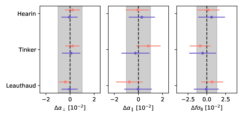
Figure 8: Best-fit values of $\alpha_{\perp}$, $\alpha_{\parallel}$ and $f{\sigma_{8}}$ from fitting the average multipoles of the OuterRim mocks compared to their average over all HOD models. Blue points show results for the CLPT-GS model and red points show results for the TNS model. The shaded area shows 1% error for $\alpha_{\perp},\alpha_{\parallel}$ and 3% for $f{\sigma_{8}}$.

4.2.4 Systematic errors from observational effects

We investigate in this section the observational systematics. We used a set of 100 EZmocks to quantify their impact on our measurements. From the same set, we added different observational effects. For simplicity, those samples were made from mocks reproducing only the eBOSS component of the survey, neglecting the CMASS component. We consider that the systematic errors estimated this way can be extrapolated to the full eBOSS+CMASS sample by assuming that their contribution is the same over the CMASS volume. We thus produced the following samples:

• no observational effects included, which we use as reference,

• including the effect of the radial integral constraint (RIC, de Mattia & Ruhlmann-Kleider, 2019), where the redshifts of the random catalog are randomly chosen from the redshifts of the data catalog,

• including RIC and all angular features: fiber collisions, redshift failures, and photometric corrections.

For each set, we computed the average multipoles and fitted them using our two RSD models. The covariance matrix is held fixed between cases. Table 9 summarises the biases in $\alpha_{\perp},\alpha_{\parallel},f{\sigma_{8}}$ caused by the different observational effects. The shifts are relative to results of mocks without observational effects. We find that the radial integral constraint produces the greatest effect, particularly for the CLPT-GS model for which the deviation on $f{\sigma_{8}}$ is slightly larger than $2\sigma$. Indeed, the quadrupole for mocks with RIC has smaller absolute amplitude, which translates into small $f{\sigma_{8}}$ values. However, when adding angular observational effects the shifts are all broadly consistent with zero, which indicates that the two effects partially cancel each other.

Using values from the Table 9 and Eqs. 43 and 44, we derive the following systematic errors from observational effects for $\alpha_{\perp}$, $\alpha_{\parallel}$ and $f{\sigma_{8}}$, respectively:

$${\rm CLPT-GS}:\sigma_{\rm syst,obs} = (0.9,\ 1.2,\ 1.7)\times 10^{-2}$$ (50)

$${\rm TNS}:\sigma_{\rm syst,obs} = (1.0,\ 1.3,\ 1.8)\times 10^{-2}$$ (51)

These systematic errors are about 50 per cent of the statistical errors for each parameter, which corresponds to the most significant contribution to the systematic error budget.

Table 9: Impact of observational effects on the full-shape analysis using Ezmocks. Each row displays the shifts of best-fit parameters with respect to the case without observational effects (“no syst”): $\Delta x=x-x^{\rm no\ syst}$. Fits are performed on the average multipoles of 100 realisations. We test the cases of mocks with radial integral constraint (RIC) and mocks with the combination of RIC and all angular observational effects (fiber collisions, redshift failures and photometric fluctuations). The angular effects introduced in mocks are corrected using the same procedure used in data. For simplicity, the mocks used here are only for the eBOSS part of the survey.

Type	Model	$\Delta\alpha_{\perp}$ [$10^{-2}$]	$\Delta\alpha_{\parallel}$ [$10^{-2}$]	$\Delta f\sigma_{8}$ [$10^{-2}$]
RIC	clpt-gs	$-0.3\pm 0.5$	$1.1\pm 0.6$	$-1.7\pm 0.8$
$+$Ang. Sys.	clpt-gs	$0.0\pm 0.4$	$0.3\pm 0.6$	$0.0\pm 0.9$
RIC	tns	$0.6\pm 0.5$	$-0.1\pm 0.7$	$-0.8\pm 0.9$
$+$Ang. Sys.	tns	$0.8\pm 0.5$	$-0.2\pm 0.7$	$0.1\pm 0.9$

4.2.5 Total systematic error of the full-shape RSD analysis

Table 10 summarises all systematic error contributions to the full-shape measurements discussed in the previous sections. We show the results for our two configuration-space RSD models TNS and CLPT-GS and for the Fourier space analysis of Gil-Marín et al. (2020). We compute the total systematic error $\sigma_{\rm syst}$ by summing up all the contributions in quadrature, assuming that they are all independent. By comparing the systematic errors with the statistical error from the baseline fits to the data (see Section 5.2), we find that the systematic errors are far from being negligible: more than 50 per cent of the statistical errors for all parameters. The systematic errors are in quadrature to the diagonal of the covariance of each measurement. We do not attempt to compute the covariance between systematic errors and this approach is more conservative (it does not underestimate errors).

Table 10: Summary of systematic errors obtained from tests with mock catalogs. The total systematic error $\sigma_{\rm syst}$ is the quadratic sum of each contribution. We compare the systematic errors to the statistical errors from our baseline fits on real data. The last rows display the final error which is a quadratic sum of statistical and systematic errors.

Type	Model	$\sigma_{\alpha_{\perp}}$	$\sigma_{\alpha_{\parallel}}$	$\sigma_{f{\sigma_{8}}}$
Modelling	clpt-gs	0.004	0.009	0.010
	tns	0.004	0.006	0.009
Fid. cosmology	clpt-gs	0.009	0.010	0.014
	tns	0.005	0.008	0.012
Obs. effects	clpt-gs	0.009	0.012	0.017
	tns	0.010	0.014	0.018
	clpt-gs	0.013	0.018	0.024
$\sigma_{\rm syst}$	tns	0.012	0.017	0.023
	$P_{\ell}$	0.012	0.013	0.024
	clpt-gs	0.020	0.028	0.045
$\sigma_{\rm stat}$	tns	0.018	0.031	0.040
	$P_{\ell}$	0.027	0.036	0.042
	clpt-gs	0.66	0.63	0.54
$\sigma_{\rm syst}/\sigma_{\rm stat}$	tns	0.65	0.55	0.58
	$P_{\ell}$	0.43	0.37	0.58
	clpt-gs	0.024	0.033	0.051
$\sigma_{\rm tot}=\sqrt{\sigma_{\rm syst}^{2}+\sigma_{\rm stat}^{2}}$	tns	0.021	0.035	0.046
	$P_{\ell}$	0.029	0.038	0.048

4.3 Statistical properties of the LRG sample

We can also use the EZmocks for evaluating the statistical properties of the LRG sample, in particular to quantify how typical is our data compared with EZmocks, but also for measuring the correlations among the different methods and globally validating our error estimation.

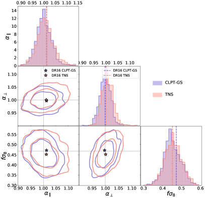
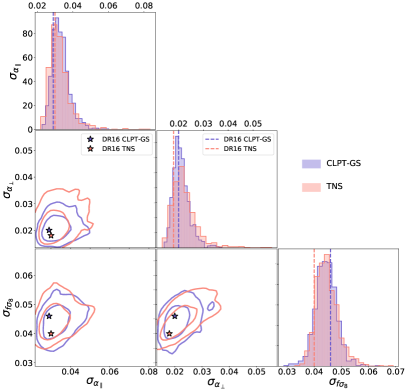
Figure 9: Comparison between best-fit values (left panels) and estimated errors (right panel) for $(\alpha_{\perp},\alpha_{\parallel},f{\sigma_{8}})$ using 1000 realisations of EZmocks fitted with the TNS and CLPT-GS models. The values obtained with real data are indicated by stars in each panel or as coloured vertical lines in the histograms. The thin black dashed line on the 2D plots refer to the true values each parameter in the EZmocks.

The left panel of the Figure 9 presents a comparison between the best-fit $(\alpha_{\perp},\alpha_{\parallel},f{\sigma_{8}})$ and their estimated errors from fits of the TNS and the CLPT-GS models. The confidence contours contain approximately 68 per cent and 95 per cent of the results around the mean. The contours and histograms reveal a good agreement for the two models. Stars indicate the corresponding best fit values obtained from the data. The correlations between best-fit parameters of both models are 86, 83 and 93 per cent for $\alpha_{\perp}$, $\alpha_{\parallel}$ and $f{\sigma_{8}}$ respectively. A similar comparison for the errors is presented in the right panel of the Figure 9. The errors inferred from the data analysis, shown as stars, are in good agreement with the 2D distributions from the mocks, lying within the 68 per cent contours. The histograms comparing the distributions of errors for both methods also show a good agreement, in particular for $\alpha_{\parallel}$ and $f\sigma_{8}$. For $\alpha_{\perp}$, we observe that the distribution from CLPT-GS is slightly peaked towards smaller errors, while for TNS the error distribution has a larger dispersion for this parameter. The correlation coefficients between estimated errors from the two models are: 56, 38, and 39 per cent for $\alpha_{\perp},\alpha_{\parallel},f{\sigma_{8}}$, respectively.

Table 11 summarizes the statistical properties of errors for ${\alpha_{\perp},\alpha_{\parallel},f{\sigma_{8}}}$ for both BAO and full shape RSD analysis in configuration space (noted $\xi_{\ell}$). We also include for reference the results from Fourier space analysis of Gil-Marín et al. (2020), noted $P_{\ell}$. For each parameter we show the standard deviation of the best fits values, $\sigma$, the mean estimated error $\langle\sigma\rangle$, the mean of the pull, $Z_{i}=(x_{i}-\langle x\rangle)/\sigma_{x}$ where $x={\alpha_{\perp},\alpha_{\parallel},f{\sigma_{8}}}$, and its standard deviation $\sigma(Z)$. If errors are correctly estimated and follow a Gaussian distribution, we expect that $\sigma=\langle\sigma_{i}\rangle$, $\langle Z_{i}\rangle=0$ and $\sigma(Z)=1$. For method, we remove results from non-converged chains and 5$\sigma$ outliers in both best-fit values and errors (with $\sigma$ defined as half of the range covered by the central 68 per cent values). Table 11 also shows the results from combining different methods employing the procedure described in Section 3.4. For each combination, we create the covariance matrix $C$ (Eq. 40) from the correlation coefficients obtained from 1000 EZmocks fits, with small adjustments to account for the observed errors of a given realisation. The correlation coefficients (before this adjustement) is shown in Figure 11 for all five methods. The BAO measurements from configuration and Fourier spaces are 87 and 88 per cent correlated for $\alpha_{\perp}$ and $\alpha_{\parallel}$, respectively. In RSD analyses these correlations reduce to slightly less than 80 per cent between $\alpha_{\perp},\alpha_{\parallel}$ of both spaces, while $f{\sigma_{8}}$ correlations reach 84 per cent. The fact that these correlations are not exactly 100 per cent indicates that there is potential gain combining them.

For the BAO results (top three rows of Table 11), we see good agreement between $\sigma_{x}$ and $\langle\sigma\rangle$ for all the parameters in both the spaces. The mean of the pull $\langle Z_{i}\rangle$ is consistent with zero (their errors are roughly 0.02) and the standard deviation $\sigma(Z_{i})$ is slightly smaller than unity for all variables, indicating that errors might be slightly overestimated. The combined BAO results of $(\xi_{\ell}+P_{\ell})$ have errors slightly reduced to 2.2% for $\alpha_{\perp}$ and 3.4% in $\alpha_{\parallel}$ (based on the scatter $\sigma$ of the best-fit values). The $\sigma(Z_{i})$ are both closer to 1.0, indicating better estimate of errors for the combined case. As a conservative approach, the BAO errors on data (Section 5.1) are therefore not corrected by this overestimation.

Full shape RSD results (4th to 8th rows in Table 11) also show good agreement between $\sigma_{x}$ and $\langle\sigma\rangle$ for all the parameters for both models and both spaces. Figure 10 shows the pull distributions for both CLPT-GS and TNS models. The mean of the pull for $\alpha_{\perp}$ and $f{\sigma_{8}}$ are consistent with zero in all cases though the mean pull for $\alpha_{\parallel}$ is negative, indicating a slightly skewed distribution. The $\sigma(Z_{i})$ values for CLPT-GS and TNS models are consistent with one for $\alpha_{\perp}$ and slightly different than one for $\alpha_{\parallel}$ and $f{\sigma_{8}}$. Their combination (6th row) with inverse variance weighing slightly compensates for these differences, yielding better estimated errors, with $\sigma(Z_{i})$ closer to one for all three parameters. The full-shape measurements in Fourier space (7th row) show similar behaviour than the ones in configuration space, with errors larger than measurements in configuration space. This is due to the larger number of nuisance parameters in the Fourier space analysis and to the choice of scales used in the Fourier space fits ($0.02\leq k\leq 0.15\ h{\rm Mpc}^{-1}$), which do not exactly translate to the range in separation used in our fits $(25<r<130$ $h^{-1}$Mpc), and may contain less information in average. The combined $\xi_{\ell}+P_{\ell}$ full-shape results in the 8th row present smaller dispersion on all parameters relative to each individual method. The pull values indicating slightly overestimated errors, which we do not attempt to correct.

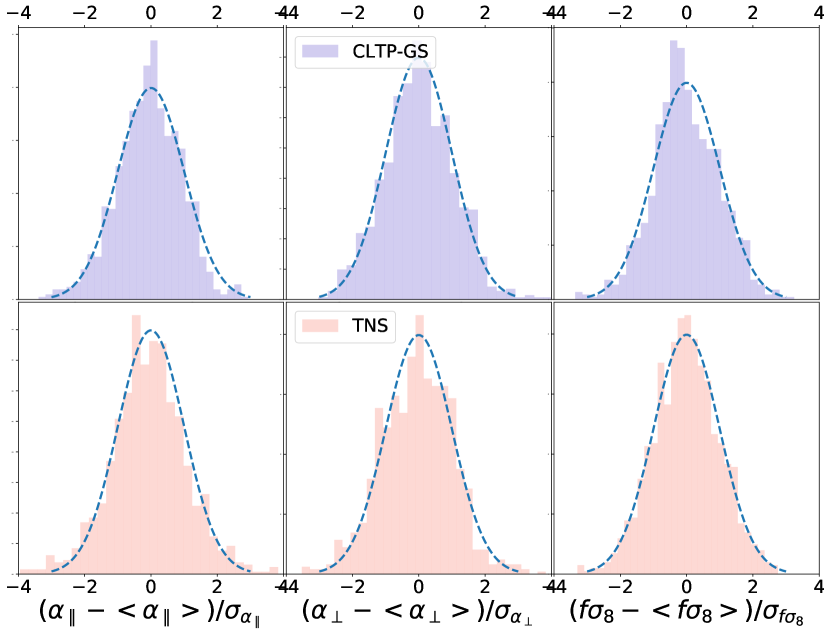
Figure 10: Normalized distributions of the pull for the $\alpha_{\parallel}$, $\alpha_{\perp}$ and $f{\sigma_{8}}$ from fits of TNS and CLPT-GS models on EZmocks. The blue dashed lines represent the centered normalized Gaussian distribution.

Table 11: Statistics on errors from consensus results on 1000 EZmocks realisations. For each parameter, we show the standard deviation of best-fit values, $\sigma(x_{i})$, the mean estimated error $\langle\sigma_{i}\rangle$, the mean of the pull, $Z_{i}=(x_{i}-\langle x_{i}\rangle)/\sigma_{i}$ and its standard deviation $\sigma(Z_{i})$. $N_{\rm good}$ shows the number of valid realisations for each case after removing extreme values and errors at 5$\sigma$ level.

Observable	$N_{\rm good}$	$\alpha_{\perp}$					$\alpha_{\parallel}$					$f{\sigma_{8}}$
		$\sigma$	$\langle\sigma_{i}\rangle$	$\langle Z_{i}\rangle$	$\sigma(Z_{i})$		$\sigma$	$\langle\sigma_{i}\rangle$	$\langle Z_{i}\rangle$	$\sigma(Z_{i})$		$\sigma$	$\langle\sigma_{i}\rangle$	$\langle Z_{i}\rangle$	$\sigma(Z_{i})$
bao $\xi_{\ell}$	987	0.023	0.023	-0.02	0.98		0.036	0.035	-0.02	0.96		-	-	-	-
bao $P_{\ell}$	978	0.024	0.024	-0.02	0.95		0.039	0.040	0.00	0.90		-	-	-	-
bao $\xi_{\ell}+P_{\ell}$	970	0.022	0.022	-0.02	1.01		0.034	0.034	-0.02	0.97		-	-	-	-
rsd $\xi_{\ell}$ clpt	819	0.023	0.021	0.01	1.03		0.033	0.033	-0.04	0.95		0.046	0.045	-0.01	0.97
rsd $\xi_{\ell}$ tns	951	0.024	0.023	-0.05	1.03		0.037	0.033	-0.05	1.07		0.046	0.045	-0.01	0.95
rsd $\xi_{\ell}$	781	0.021	0.021	-0.01	0.99		0.031	0.032	-0.03	0.96		0.042	0.045	-0.01	0.95
rsd $P_{\ell}$	977	0.025	0.026	0.02	0.94		0.037	0.036	-0.04	1.00		0.046	0.046	0.01	0.96
rsd $\xi_{\ell}+P_{\ell}$	767	0.019	0.020	0.00	0.98		0.030	0.031	-0.03	0.97		0.041	0.043	-0.00	0.97
bao$+$rsd $\xi_{\ell}$	772	0.018	0.019	-0.01	1.00		0.024	0.025	-0.03	0.97		0.043	0.040	-0.02	1.06
bao$+$rsd $P_{\ell}$	955	0.019	0.020	0.00	0.96		0.028	0.029	-0.03	0.96		0.044	0.042	-0.01	1.05
bao$\times$rsd $P_{\ell}$	986	0.019	0.019	0.03	0.99		0.029	0.028	-0.06	1.02		0.041	0.045	-0.01	0.92
bao ($\xi_{\ell}+P_{\ell}$) +	747	0.017	0.018	-0.01	1.00		0.024	0.025	-0.03	0.97		0.042	0.039	-0.02	1.09
rsd ($\xi_{\ell}+P_{\ell}$)
(bao$+$rsd) $\xi_{\ell}$ +	747	0.017	0.018	-0.01	1.01		0.024	0.025	-0.03	0.99		0.042	0.039	-0.02	1.09
(bao$+$rsd) $P_{\ell}$

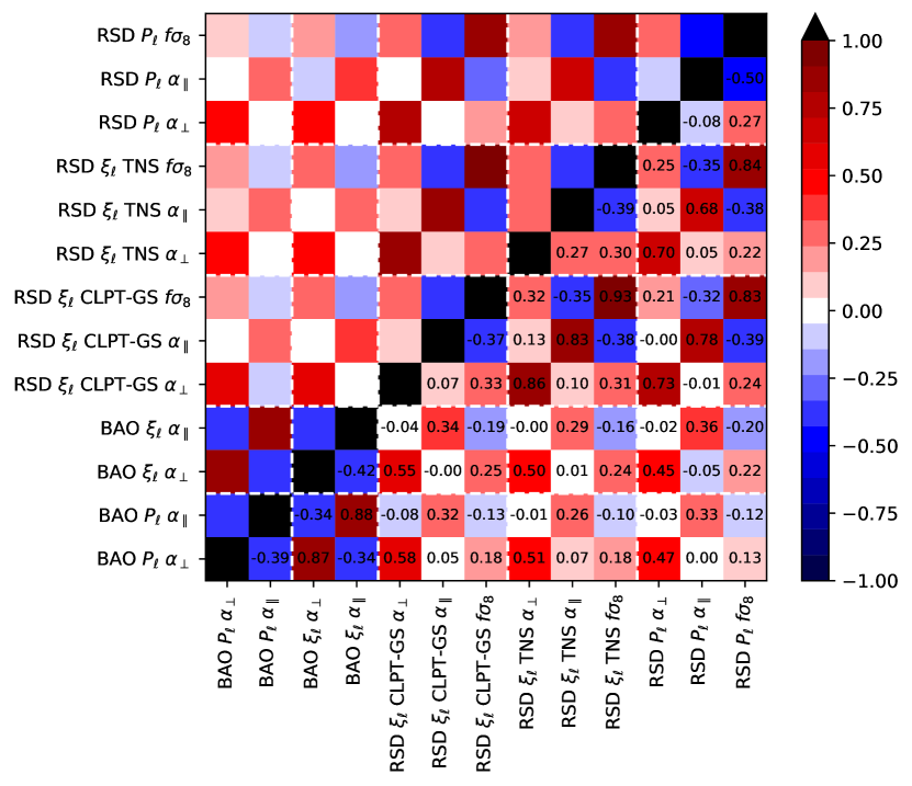
Figure 11: Correlation coefficients between $\alpha_{\perp},\alpha_{\parallel},f{\sigma_{8}}$ for all methods and models obtained from fits to 1000 EZmock realisation of the eBOSS LRG+CMASS sample. The values of $f{\sigma_{8}}$ have been corrected with the procedure described in Section 3.2.4.

The 9th and 10th row of Table 11 show results of combining BAO and full-shape RSD results for a given space, $\xi_{\ell}$ or $P_{\ell}$, while fully accounting for their large covariance as described in Section 3.4. We see that the scatter of $\alpha_{\perp}$ and $\alpha_{\parallel}$ is reduced by $\sim$ 20 and 30 per cent, respectively, relative to their BAO-only analyses. For $f{\sigma_{8}}$ the scatter of best-fit values is the same as the full-shape-only analyses, as expected (BAO only do not provide extra information on $f{\sigma_{8}}$). The values of $\sigma(Z_{i})$ for the combined results are consistent with one for $\alpha_{\perp},\alpha_{\parallel}$, though for $f{\sigma_{8}}$ they are more than 5 per cent larger than unity for both configuration and Fourier space. This would indicate that our combination procedure from Section 3.4 produces slightly underestimated errors for $f{\sigma_{8}}$. In Gil-Marín et al. (2020), an alternative method was suggested to extract the consensus results from BAO and RSD analysis: a simultaneous fit. Both BAO and RSD models are fitted simultaneously to the concatenation of the pre- and post-reconstruction data vectors. This fit requires the full covariance matrix between pre- and post-reconstruction multipoles and is estimated from 1000 EZmocks. Results of simultaneous fits on mocks are shown in the 11th row of Table 11 and are noted “BAO$\times$RSD $P_{\ell}$”. These are to be compared with our usual method of combining posteriors, noted “BAO$+$RSD” and shown in the 10th row. First, we see good agreement between the scatter of best-fit values of all three parameters between BAO$\times$RSD and BAO$+$RSD. However, the simultaneous fit overestimates the errors in $f{\sigma_{8}}$ by 8 per cent, based on its $\sigma(Z_{i})$ value. While in theory the simultaneous fit is a better procedure, accounting for all correlations, in practice we only use 1000 mocks to estimate a larger covariance matrix with large off-diagonal terms. Therefore we cannot conclude from this test, which method leads to better estimated errors. We use BAO$+$RSD entries for the consensus results.

The last two rows of Table 11 show statistics on the final consensus results from the LRG sample when combining BAO and full shape from both Fourier and configuration spaces. These results reflect the full statistical power of the LRG sample. The excellent agreement between the statistics of these two rows shows that the order of combination does not impact results. The dispersion $\sigma$ on $\alpha_{\perp}$ and $\alpha_{\parallel}$ are reduced to 1.8 and 2.6 per cent respectively while we had 2.2 and 3.4 per cent for BAO only, and 2.0 and 3.2 per cent for full-shape only. The pull distributions for $\alpha_{\perp}$ and $\alpha_{\parallel}$ are consistent with a Gaussian distribution. The scatter in $f{\sigma_{8}}$ is not reduced compared to individual methods, which is expected since BAO does not add information on this parameter, so the consensus error should be equal to the one obtained from the full-shape fits. However, the $\sigma(Z_{i})$ for $f{\sigma_{8}}$ indicates that our consensus errors on this parameter might be underestimated by 10 per cent. While this seems to be significant, this result can be a consequence of the Gaussian assumption of all individual likelihoods not holding for all realisations, or the combination procedure itself might lead to underestimated errors (as seen with $f{\sigma_{8}}$ in the 9th and 10th rows), though we would need more mocks to test these hypotheses carefully.

For this work, we consider the underestimation on $f{\sigma_{8}}$ consensus errors (last two rows of Table 11) as another source of systematic error. The simplest correction to this underestimation is to scale the estimated errors of $f{\sigma_{8}}$ in each realisation by $\sigma(Z_{i})=1.09$. We proceed to apply this correction factor to the consensus $f{\sigma_{8}}$ errors with our data sample. This factor is to be applied only to statistical errors. In Section 5.3 we describe how we apply with this scaling in the presence of systematic errors.

5 Results

We provide in this section the results of the BAO analysis, the full-shape RSD analysis and the combination of the two for the eBOSS LRG sample. The analysis assumes an effective redshift for the sample of $z_{\rm eff}=0.698$.

5.1 Result from the BAO analysis

We present in Figure 12 our best-fit BAO model to the post-reconstruction eBOSS LRG multipoles. The associated reduced chi-squared is $\chi^{2}/{\rm dof}=39/(40-9)=1.26$. By scaling the resulting $\alpha_{\perp}$ and $\alpha_{\parallel}$ by $(D_{M}/r_{d})^{\rm fid}$ and $(D_{H}/r_{d})^{\rm fid}$, respectively (Eqs. 7 and 8), we obtain:

$$\mathbf{D}_{{\rm BAO},{\xi_{\ell}}}=\begin{pmatrix}D_{M}/r_{d}\\ D_{H}/r_{d}\end{pmatrix}=\begin{pmatrix}17.86\pm 0.33\\ 19.34\pm 0.54\end{pmatrix}$$ (52)

and the covariance matrix is

$$\mathbf{C}_{{\rm BAO},{\xi_{\ell}}}=\blockarray{cc}D_{M}/r_{d}&D_{H}/r_{d}\vspace{1mm}\\ \block{(cc)}1.11\times 10^{-1}-5.86\times 10^{-2}\\ -2.92\times 10^{-1}\\$$ (53)

The errors correspond to a BAO measurement at 1.9 per cent in the transverse direction and 2.8 per cent in the radial direction, the best constraints ever obtained from $z>0.6$ galaxies. The correlation coefficient between both parameters is -0.33.

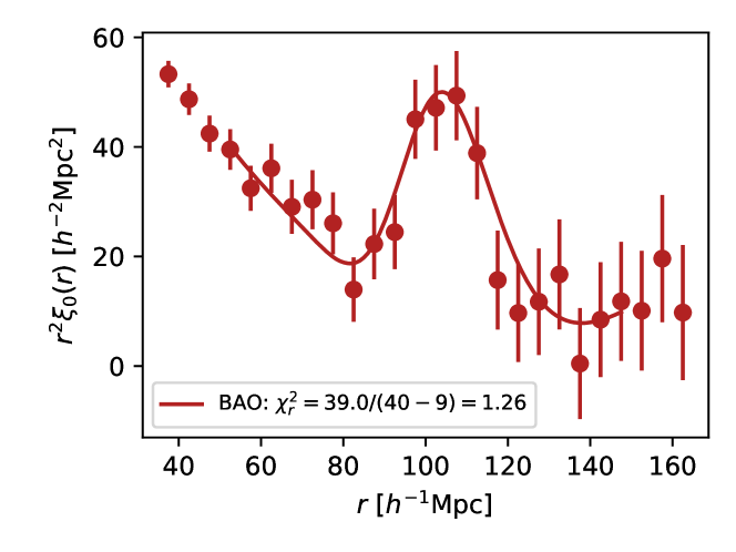
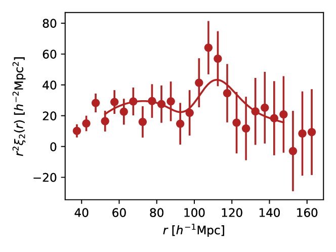
Figure 12: Best-fit BAO model to the monopole (top) and quadrupole (bottom) of the post-reconstruction correlation function of the eBOSS + CMASS LRG sample. The legend displays the $\chi^{2}$ value of the fit.

Figure 13 shows in blue the 68 and 95% confidence contours in the $(D_{M}/r_{d},D_{H}/r_{d})$ space for the BAO measurement in configuration space. Our best-fit values are consistent within 1.26$\sigma$ to the prediction of a flat $\Lambda$CDM model given by Planck 2018 best-fit parameters (Collaboration et al., 2018b) assuming a $\chi^{2}$ distribution with two degrees of freedom. This measurement is also in excellent agreement with the BAO analysis performed in Fourier space (Gil-Marín et al., 2020), shown as red contours in Figure 13. Since Fourier and configuration space analyses use the same data, final measurements are highly correlated. Based on measurements of the same 1000 realisations of EZmocks, we obtain correlation coefficients of 0.86 for both $D_{M}/r_{d}$ and $D_{H}/r_{d}$. As these correlations are not unity, there is some gain, in combining both measurements. Using the methods presented in Section 3.4, we compute the combined BAO measurements between Fourier and configuration space. The result is displayed as grey contours in Figure 13 and in Table 14 as “BAO $\xi_{\ell}+P_{\ell}$”. The error of the combined result is only 2% smaller than the error of the configuration space analysis alone.

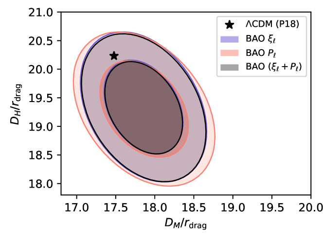
Figure 13: Constraints on $D_{M}/r_{d}$ and $D_{H}/r_{d}$ at $z_{\rm eff}=0.698$ from the BAO analysis of the eBOSS LRG sample post-reconstruction. Contours show 68 and 95 per cent confidence regions for the configuration space analysis in blue (this work), the Fourier space analysis from Gil-Marín et al. (2020) in salmon, and the consensus BAO result in grey. The expected values in a flat $\Lambda$CDM model with Planck 2018 best-fit parameters, shown by the black star, lies at 1.26$\sigma$ from our best-fit parameters of the configuration space analysis.

Table 12 shows the impact on the BAO results in configuration space of different modifications in the methodology around the baseline configuration. The middle part of the table shows that our result is reasonably insensitive to some of these changes. Setting all systematic weights to unity causes only mild shifts to best-fit parameters while estimated errors are unchanged. Removing the corrections by weights significantly distorts the broad shape of the correlation function. The fact that our BAO results are insensitive to these corrections proves that practically all information comes uniquely from the BAO peak and not from the full-shape of the correlation function. This is a strong robustness validation of our BAO measurement. When leaving BAO damping parameters $(\Sigma_{\perp},\Sigma_{\parallel})$ free or constrained within a Gaussian prior, the best-fit values barely change while their errors are smaller than our baseline analysis. As observed on mocks, some realisations present sharper peaks due to noise and a sharper model could be considered as a better fit. However, we prefer to be conservative and not allow for this artificial increase in precision in our BAO analysis. Including the hexadecapole or changing the fiducial cosmology shifts alphas by less than one error bar, which is consistent to what is observed in mocks. We performed the BAO fits using the methods used in the BOSS DR12 analysis (Alam et al., 2017) which gives results in excellent agreement with our baseline method, with a slight better $\chi^{2}$. In the third part of Table 12 we present the pre-reconstruction result with similar best-fit $\alpha_{\perp}$ and $\alpha_{\parallel}$ but with errors larger by factors of 1.3 and 1.5, which is typical as seen in mocks (Figure 5). Pre-reconstruction BAO-only fits using our methodology show biases of about 1 per cent in the mocks, therefore we do not recommend using pre-reconstruction results without accounting for these biases. The NGC and SGC results are two independent samples and their best-fit $\alpha_{\perp}$ and $\alpha_{\parallel}$ are 0.25 and 0.53$\sigma$ from each other respectively, therefore not representing a significant difference among hemispheres.

Table 12: The BAO measurement with the DR16 eBOSS+CMASS LRG dataset using the standard pipeline described in Section 3.1 and other analysis choices. Note that for cases with different $\Omega_{m}^{\rm fid}$, we scale the obtained $\alpha_{\perp},\alpha_{\parallel}$ by the distance ratios in order to make them comparable with the case where $\Omega_{m}^{\rm fid}=0.31$.

case	$\alpha_{\perp}$	$\alpha_{\parallel}$	$\chi^{2}/{\rm d.o.f.}$
Baseline	$1.024\pm 0.019$	$0.956\pm 0.023$	$39.0/(40-9)$
$w_{\rm sys}w_{\rm cp}w_{\rm noz}=1$	$1.022\pm 0.018$	$0.954\pm 0.023$	$30.1/(40-9)$
$\Sigma_{\perp},\Sigma_{\parallel}$ free	$1.027\pm 0.016$	$0.947\pm 0.019$	$31.9/(40-11)$
$\Sigma_{\perp},\Sigma_{\parallel}$ prior	$1.025\pm 0.017$	$0.952\pm 0.021$	$36.2/(40-11)$
$+\xi_{4}$	$1.031\pm 0.019$	$0.949\pm 0.024$	$53.5/(60-12)$
$\Omega_{m}^{\rm fid}=0.27$	$1.026\pm 0.020$	$0.950\pm 0.023$	$33.3/(40-9)$
$\Omega_{m}^{\rm fid}=0.35$	$1.026\pm 0.019$	$0.951\pm 0.022$	$39.6/(40-9)$
DR12 method	$1.023\pm 0.019$	$0.955\pm 0.024$	$34.5/(40-10)$
Pre-recon	$1.035\pm 0.025$	$0.957\pm 0.035$	$42.0/(40-9)$
NGC only	$1.038\pm 0.024$	$0.943\pm 0.024$	$42.3/(40-9)$
SGC only	$0.993\pm 0.032$	$0.982\pm 0.070$	$44.5/(40-9)$

5.2 Results from the full-shape RSD analysis

Table 13: The full-shape measurements with the DR16 eBOSS+CMASS LRG dataset from our baseline analysis described in Section 3.2 followed by results from other analysis choices. The presented errors are purely statistical and do not include systematic errors.

Model	Analysis	$\alpha_{\perp}$	$\alpha_{\parallel}$	$f\sigma_{8}$	$\chi^{2}/{\rm d.o.f.}$
CLPT-GS	baseline	$0.997\pm 0.020$	$1.013\pm 0.028$	$0.471\pm 0.045$	$83.7/(63-6)=1.47$
CLPT-GS	$r_{\rm min}=35$$h^{-1}$Mpc for $\xi_{4}$	$1.017\pm 0.022$	$0.971\pm 0.031$	$0.499\pm 0.046$	$79.3/(61-6)=1.44$
CLPT-GS	NGC only	$1.015\pm 0.025$	$1.009\pm 0.031$	$0.464\pm 0.055$	$81.1/(63-6)=1.40$
CLPT-GS	SGC only	$0.985\pm 0.036$	$1.041\pm 0.062$	$0.439\pm 0.078$	$71.3/(63-6)=1.25$
TNS	baseline	$1.001\pm 0.018$	$1.013\pm 0.031$	$0.451\pm 0.040$	$85.2/(65-7)=1.47$
TNS	$r_{\rm min}=35$$h^{-1}$Mpc for $\xi_{4}$	$1.013\pm 0.016$	$0.976\pm 0.027$	$0.458\pm 0.036$	$73.7/(63-7)=1.32$
TNS	Without $\xi_{4}$	$1.019\pm 0.019$	$0.963\pm 0.035$	$0.472\pm 0.044$	$50.1/(44-7)=1.35$
TNS	NGC only	$1.024\pm 0.029$	$1.013\pm 0.036$	$0.436\pm 0.053$	$80.6/(65-7)=1.39$
TNS	SGC only	$0.993\pm 0.034$	$1.076\pm 0.070$	$0.423\pm 0.076$	$69.1/(65-7)=1.19$

We present in Figure 14 the best-fit TNS (red) and CLPT-GS (blue) RSD models to the pre-reconstruction eBOSS LRG multipoles. The associated reduced chi-squared values are $\chi^{2}/{\rm dof}=85.2/(65-7)=1.47$ for TNS and $\chi^{2}/{\rm dof}=83.7/(63-6)=1.47$ for CLPT-GS. While these values are unlikely explained by statistical fluctuations, we verified that the values reported for the $\chi^{2}$ for both models are within EZmock $\chi^{2}$ distributions. Both models perform similarly on data, but some differences are visible in Figure 14. The TNS model produces a slightly sharper BAO peak than the CLPT-GS model, clearly visible in the monopole. This is due the fact that, intrinsically, the CLPT-GS model tends to predict a slighter higher BAO damping compared to Eulerian perturbation theory, as implemented here in the TNS model with RESPRESSO prescription. The CLPT-GS model have a slightly higher hexadecapole amplitude than the TNS model but both models seems to underestimate the hexadecapole amplitude below 35 $h^{-1}$Mpc by 1$\sigma$ of the statistical uncertainties of the data. This underestimation in the amplitude of the hexadecapole is also present in the mocks for both the Nseries and EZmocks and was already reported in Icaza-Lizaola et al. (2020) explaining the relative high $\chi^{2}$ of the data.

Table 13 shows the impact of different modifications in the methodology around the baseline configuration. First, if we change the range of scales used in the hexadecapole by changing $r_{\rm min}$ from 25$h^{-1}$Mpc to 35$h^{-1}$Mpc. We see a decrease of the reduced chi-squared as we remove these scales from the hexedecapole, which are underestimated by the models. Removing those scales impact the measured cosmological parameters, particularly $\alpha_{\parallel}$, which is shifted by about 1 $\sigma$. We performed the same cuts on the analysis of EZmocks, finding that such a shift lies at about 2.3$\sigma$ of the shifts observed in 1000 mocks (see details in Appendix 21). The NGC and SGC fields are two independent samples and we find that their individual best-fit $\alpha_{\perp}$ and $\alpha_{\parallel}$, and $f\sigma_{8}$ are 0.7$\sigma$, $0.5\sigma$ and 0.3$\sigma$ from each other respectively for CLPT-GS and 0.7$\sigma$, $0.8\sigma$ and 0.1$\sigma$ for TNS, which is not a significant difference.

The marginal posteriors on $\alpha_{\perp},\alpha_{\parallel},f{\sigma_{8}}$ and associated 68% and 95% confidence contours are shown in Figure 15. The posteriors obtained from both models are in good agreement. Entries denoted as “RSD $\xi_{\ell}$ CLPT-GS” and “RSD $\xi_{\ell}$ TNS” in Table 14 gives the best-fit parameters and 1$\sigma$ error (including systematic errors), translated into $D_{M}/r_{d},D_{H}/r_{d},f{\sigma_{8}}$. We find an excellent agreement in the best-fit parameters and errors between the two RSD models, as expected from the posteriors. The full posteriors including all nuisance parameters can be found in Appendix C.

We combine the results from our two RSD models using a weighted average based on the individual covariance matrices (see Section 3.4). The combined measurement is indicated by “RSD $\xi_{\ell}$” in Table 14 and shown with dashed contours in Figure 15. Central values and errors of the combined result fall approximately in between the values of each individual measurement.

The combined best-fit parameters and covariance matrix of the full-shape RSD analysis in configuration space, including systematic errors, are

$$\mathbf{D}_{{\rm RSD},{\xi_{\ell}}}=\begin{pmatrix}D_{M}/r_{d}\\ D_{H}/r_{d}\\ f\sigma_{8}\end{pmatrix}=\begin{pmatrix}17.42\pm 0.40\\ 20.46\pm 0.70\\ 0.460\pm 0.050\end{pmatrix}$$ (54)

$$\mathbf{C}_{{\rm RSD},{\xi_{\ell}}}=\blockarray{ccc}D_{M}/r_{d}&D_{H}/r_{d}f{\sigma_{8}}\vspace{1mm}\\ \block{(ccc)}1.59\times 10^{-1}6.28\times 10^{-3}6.13\times 10^{-3}\\ -4.88\times 10^{-1}-4.83\times 10^{-3}\\ --2.46\times 10^{-3}\\$$ (55)

This corresponds to a 2.3 and 3.4 per cent measurements of the transverse and radial dilation parameters and a 11 per cent measurement of the growth rate of structure times $\sigma_{8}$. The errors on $D_{M}/r_{d}$ and $D_{H}/r_{d}$ are slightly larger than the ones from the BAO-only analysis, as expected, but the correlation coefficient between them is reduced from $-0.33$ to $0.02$. This happens because information on dilation parameters also come from the full-shape of the correlation function, rather than just the BAO peak. For instance, the correlation coefficient between $f{\sigma_{8}}$ and $D_{M}/r_{d}$ is 0.31 and between $f{\sigma_{8}}$ and $D_{H}/r_{d}$ is -0.14.

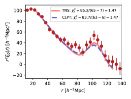
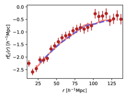
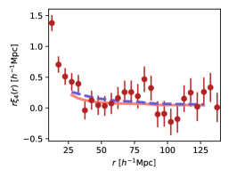
Figure 14: Best-fits full-shape models to the eBOSS + CMASS multipoles. Left, mid and right panel display mono, quad and hexadecapole, respectively. The monopole is scaled by $r^{2}$ while the other two are scaled by $r$. The CLPT-GS model is shown by the blue dashed line while the TNS model is shown by the red solid line. Note the baseline ranges used for each model are slightly different (see Figure 6).

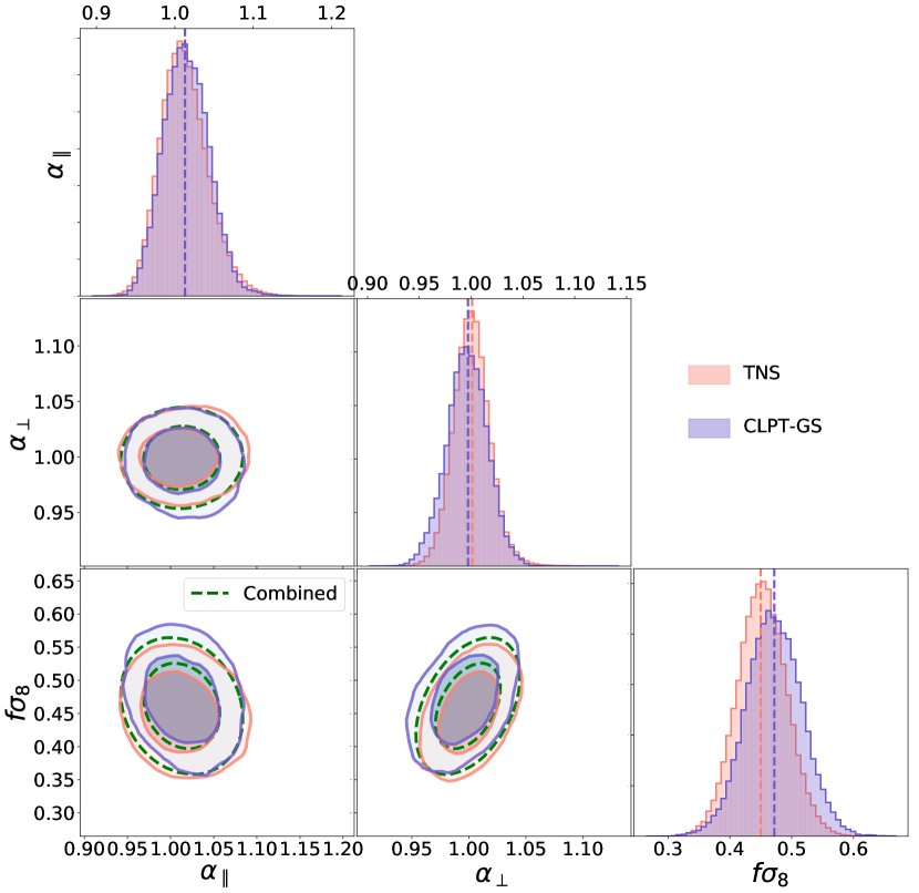
Figure 15: Comparison between the TNS and CLPT-GS final posterior distributions over the three main parameters using the DR16 data. The distributions are in good agreement for the two models. The vertical dashed lines on the 1D distributions refer to the mean. Dashed line contours show the combined result from the two models, assumming Gaussian errors. The full posteriors including nuisance parameters can be found in Appendix C.

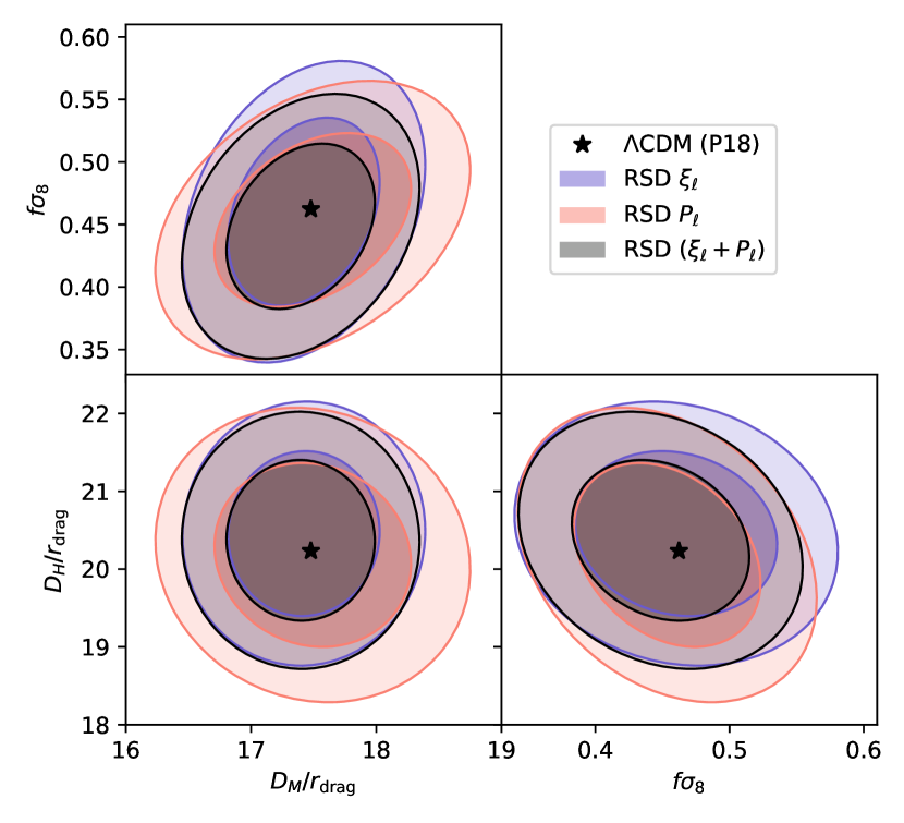
Figure 16: Constraints on $D_{M}/r_{d},D_{H}/r_{d}$ and $f{\sigma_{8}}$ $z_{\rm eff}=0.698$ from the full-shape RSD analysis of the completed eBOSS LRG sample pre-reconstruction. Contours show 68 and 95 per cent confidence regions for the analyses in configuration space (blue), Fourier space (red) and the combined (grey). The expected values in a flat $\Lambda$CDM model with best-fit parameters from Planck 2018 results is indicated as a black star.

5.3 Consensus Results

We present in Figure 17 the final results of this work obtained by the combination of BAO and full-shape RSD analyses in both configuration and Fourier spaces. Accounting for all sources of systematic error discussed in Section 4.2 and 4.3, the best-fit parameters and associated covariance matrix are:

$$\mathbf{D}_{{\rm LRG}}=\begin{pmatrix}D_{M}/r_{d}\\ D_{H}/r_{d}\\ f{\sigma_{8}}\end{pmatrix}=\begin{pmatrix}17.65\pm 0.30\\ 19.77\pm 0.47\\ 0.473\pm 0.044\end{pmatrix}$$ (56)

$$\mathbf{C}_{{\rm LRG}}=\blockarray{ccc}D_{M}/r_{d}&D_{H}/r_{d}f{\sigma_{8}}\vspace{1mm}\\ \block{(ccc)}9.11\times 10^{-2}-3.38\times 10^{-2}2.47\times 10^{-3}\\ -2.20\times 10^{-1}-3.61\times 10^{-3}\\ --1.96\times 10^{-3}\\$$ (57)

which translate into a 1.7 and 2.4 per cent measurement of $D_{M}/r_{d}$ and $D_{H}/r_{d}$ respectively. The correlation between these two is $-24$ per cent. The error on $f{\sigma_{8}}$ is 9.4 per cent, which is the most precise measurement to date in this redshift range. We note that this final measurement is not sensitive to the order of combinations, as seen in the second panel of Figure 17 and in the last row of Table 14. Those measurements agree well with the predictions from Collaboration et al. (2018a), which predict at this redshift: 17.48, 20.23 and 0.462, respectively, for a flat $\Lambda$CDM model assuming gravity is described by General Relativity. These values are shown as stars in Figure 17.

Systematic errors originating from observational effects, modelling and combination methods were carefully included in our measurements and are responsible for inflating final errors by 6, 13 and 20 per cent, respectively, on $D_{M}/r_{d},D_{H}/r_{d}$ and $f{\sigma_{8}}$. In Section 4.3, we found that our statistical errors on the consensus $f{\sigma_{8}}$ were slightly underestimated. To apply this correction on the data consensus, we proceed as follows. First, we compute consensus with and without accounting for systematic errors from Table 10. The difference between their error matrices gives us the additive systematic matrix. Then, we scale the statistical errors on $f{\sigma_{8}}$ by 1.09 and we add back the additive systematic matrix. This procedure yields the results reported in Eq. 56 and 57.

Table 14: Summary table with results from this work, from Gil-Marín et al. (2020), and their combination. All reported errors include the systematic component. The effective redshift of all measurements is $z_{\rm eff}=0.698$.

Method	$D_{M}/r_{d}$	$D_{H}/r_{d}$	$f\sigma_{8}$
bao $\xi_{\ell}$	$17.86\pm 0.33$	$19.34\pm 0.54$	-
bao $P_{\ell}$	$17.86\pm 0.37$	$19.30\pm 0.56$	-
bao $\xi_{\ell}+P_{\ell}$	$17.86\pm 0.33$	$19.33\pm 0.53$	-
rsd $\xi_{\ell}$ clpt	$17.39\pm 0.43$	$20.46\pm 0.68$	$0.471\pm 0.052$
rsd $\xi_{\ell}$ tns	$17.45\pm 0.38$	$20.45\pm 0.72$	$0.451\pm 0.047$
rsd $\xi_{\ell}$	$17.42\pm 0.40$	$20.46\pm 0.70$	$0.460\pm 0.050$
rsd $P_{\ell}$	$17.49\pm 0.52$	$20.18\pm 0.78$	$0.454\pm 0.046$
rsd $\xi_{\ell}+P_{\ell}$	$17.40\pm 0.39$	$20.37\pm 0.68$	$0.449\pm 0.044$
bao$+$rsd $\xi_{\ell}$	$17.65\pm 0.31$	$19.81\pm 0.47$	$0.483\pm 0.047$
bao$+$rsd $P_{\ell}$	$17.72\pm 0.34$	$19.58\pm 0.50$	$0.474\pm 0.042$
bao ($\xi_{\ell}+P_{\ell}$) $+$	$17.65\pm 0.30$	$19.77\pm 0.47$	$0.473\pm 0.044$
rsd ($\xi_{\ell}+P_{\ell}$)
(bao$+$rsd) $\xi_{\ell}$ $+$	$17.64\pm 0.30$	$19.78\pm 0.46$	$0.470\pm 0.044$
(bao$+$rsd) $P_{\ell}$

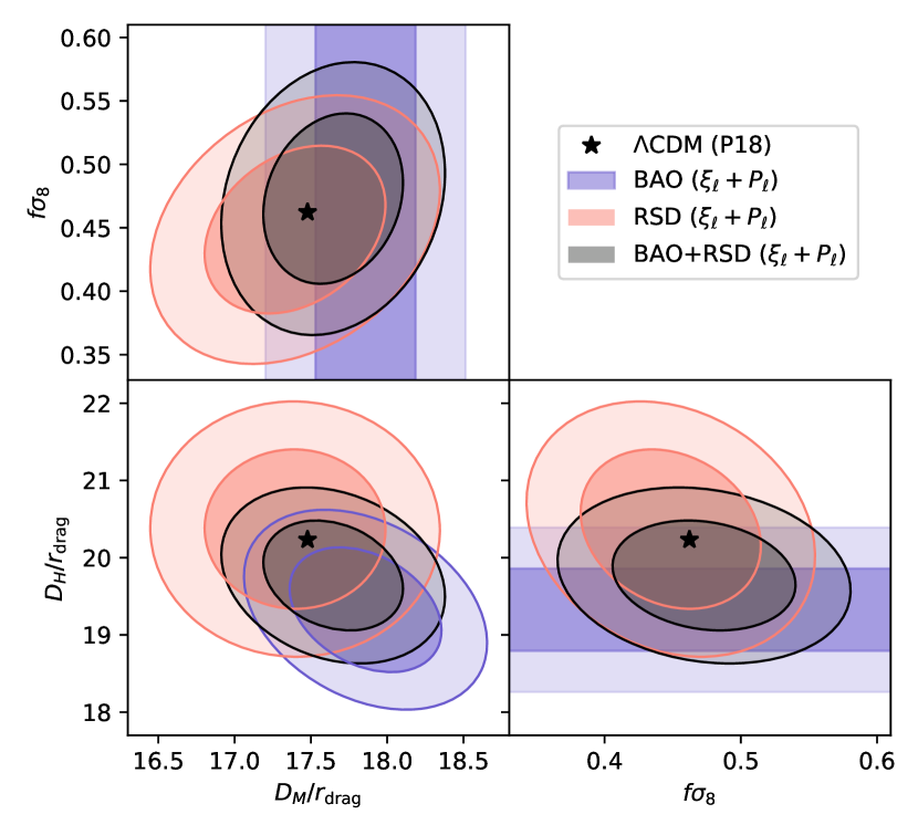
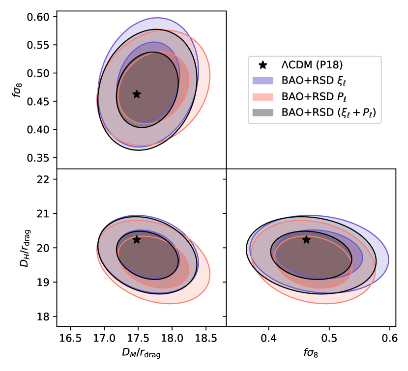
Figure 17: Final measurements of $D_{M}/r_{d},D_{H}/r_{d},f{\sigma_{8}}$ from the completed eBOSS LRG sample at $z_{\rm eff}=0.698$. Top and bottom panels show two possible procedures for obtaining the final result. The grey contours show the final results, which virtually the same in both panels (two bottom lines in Table 14). The black star indicates the prediction in a flat $\Lambda$CDM model with parameters from Planck 2018 results.

5.4 Comparison with previous results

Our final consensus result for the DR16 LRG sample is shown in Eqs. 56 and 57, and used a total of 402,052 (weighted) galaxies over 9,463 deg² (with 4,242 deg² observed by eBOSS). Bautista et al. (2018) and Icaza-Lizaola et al. (2020) describe, respectively, the BAO and full-shape RSD measurements using the DR14 LRG sample, that contains 126,557 galaxies over 1,844 deg². In the DR14 sample, CMASS galaxies outside of the eBOSS footprint were not used. Because of that, the effective redshift of the DR14 measurements is slightly higher, at $z_{\rm eff}=0.72$.

Bautista et al. (2018) reported a 2.5 per cent measurement of the ratio of the spherically averaged distance to the sound horizon scale, $D_{V}(z=0.72)/r_{d}=16.08^{+0.41}_{-0.40}$. This result was obtained with isotropic fits to the monopole of the post-reconstruction correlation function. The statistical power of the DR14 sample is relatively low for anisotropic BAO constraints and has large non-Gaussian errors. Converting our DR16 anisotropic measurement of Eq. 56 into spherically averaged distances we obtain: $D_{V}(z=0.698)/r_{d}=16.26\pm 0.20$, which is well within 1$\sigma$ from the DR14 value. The error on $D_{V}$ has reduced by a factor of two, slightly more than the square-root of the increase in effective volume, which gives a factor of $\sqrt{V_{\rm eff,DR16}/V_{\rm eff,DR14}}=\sqrt{2.73/0.9}\sim 1.74$. Note that in DR16 we combine BAO and full-shape analysis in Fourier and configuration spaces, which maximizes the amount of extracted cosmological information.

Icaza-Lizaola et al. (2020) presented the full-shape RSD analysis in the DR14 LRG sample in configuration space, yielding $f\sigma_{8}=0.454\pm 0.134$, $D_{M}/r_{d}=17.07\pm 1.55$, and $D_{H}/r_{d}=19.17\pm 2.84$. All values are consistent within 1$\sigma$ of DR16 results, even though errors for DR14 are quite large given the even lower significance of the BAO peak in the pre-reconstruction multipoles. The error on the growth rate of structure $f{\sigma_{8}}$ reduces by a factor of 3 in DR16 compared to DR14, clearly benefiting from the larger sample and the combination with post-reconstruction BAO results that help breaking model degeneracies.

Our DR16 LRG results at $0.6<z<1.0$ supersede the highest redshift results of the DR12 BOSS sample at $0.5<z<0.75$, which has an effective redshift of $z_{\rm eff}=0.61$. Alam et al. (2017) report a 1.4, 2.2 and 7.8 per cent measurements of $D_{M}/r_{d},D_{H}/r_{d}$ and $f{\sigma_{8}}$ respectively. While the errors in the high-redshift bin are slightly smaller than our DR16 result, it has a large correlation with the intermediate-redshift bin at $0.4<z<0.6$. Our DR16 measurement is thus virtually independent of the first two DR12 BOSS redshift bins, and has effectively more weight in the final joint cosmological constraints. The cosmological implications of our DR16 LRG measurements are fully described in eBOSS collaboration (2020).

6 Conclusion

This work presented the cosmological analysis of the configuration-space anisotropic clustering in the DR16 eBOSS LRG sample, which is used for the final cosmological analysis of the completed eBOSS survey. We extracted and model the BAO and RSD features from the galaxy two-point correlation function monopole, quadrupole, and hexadecapole moments. We used the reconstruction technique to sharpen the BAO peak and mitigate associated non-linearies. The pre- and post-reconstruction multipole moments were used to perform a full-shape RSD analysis and a BAO-only analysis, respectively. In the RSD analysis, we considered two different RSD models, which results were later combined to increase the robustness and accuracy of the measurements. The combination of the BAO-only and full-shape RSD analyses allowed us to derive joint constraints on the three cosmological parameter combinations: $D_{H}(z)/r_{d}$, $D_{M}(z)/r_{d}$ and $f\sigma_{8}(z)$. This analysis is complementary to that performed in Fourier space and presented in Gil-Marin et al. 2020. We found an excellent agreement between the inferred parameters in both spaces, both for BAO-only and full-shape RSD analyses. After combining the results with those from that in Fourier space, we obtain the following final constraints: $D_{M}/r_{d}=17.65\pm 0.30$, $D_{H}/r_{d}=19.77\pm 0.47$, $f{\sigma_{8}}=0.473\pm 0.044$, which are currently the most accurate at $z_{\rm eff}=0.698$.

The adopted methodology has been extensively tested on a set of realistic simulations and shown to be very robust against systematics. In particular, we investigated different potential sources of systematic errors: inaccuracy in the modelling of both BAO/RSD and intrinsic galaxy clustering, arbitrary choice of reference cosmology, and systematic errors from observational effects such as redshift failures, fiber collision, incompleteness, or the radial integral constraint. We quantified the associated systematic error contributions and included them on the final cosmological parameter constraints. Overall, we found that the total systematic error inflate errors by 6, 13 and 20 per cent for $\alpha_{\perp}$, $\alpha_{\parallel}$ and $f{\sigma_{8}}$.

The cosmological parameters inferred from the DR16 eBOSS LRG sample are in good agreement with the predictions from General Relativity in a flat $\Lambda$CDM cosmological model with parameters set to Planck 2018 results. These measurements complement those obtained from the other eBOSS tracers (Raichoor et al., 2020; de Mattia et al., 2020; Hou et al., 2020; Neveux & Burtin, 2020; du Mas des Bourboux et al., 2020). The full cosmological interpretation of all eBOSS tracer results and combined with previous BOSS results is presented in eBOSS collaboration (2020).

Future large spectroscopic surveys such as DESI or Euclid will probe much larger volumes of the Universe. This will allow reducing the statistical errors on the cosmological parameters considerably, at the percent level or below. For those it will be crucial to control the level of systematics at a extremely low level. This is today a challenge and the work presented here has shown the current state-of-the-art methodology, which will have to be further developed and improved in view of the optimal exploitation of next-generation surveys.

Data Availability

The correlation functions, covariance matrices, and resulting likelihoods for cosmological parameters are (will be made) available (after acceptance) via the SDSS Science Archive Server (https://sas.sdss.org/), with the exact address tbd.

Appendix A Impact of scales used from the hexacadecapole

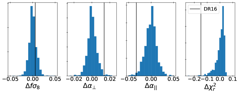
Figure 18: Variation of the cosmological parameters and the reduced chi-squared as a function of the truncation scale of the hexadecapole for the TNS model. The normalisazed distributions corresponds to 1000 EZmocks while the vertical lines corresponds to the shift for the data.

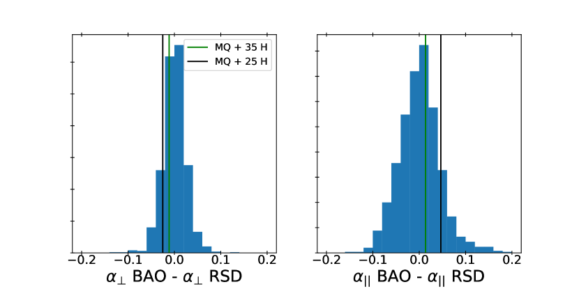
Figure 19: Absolute difference between TNS and BAO post recon constraint on the alphas. The normalisazed distributions corresponds to 1000 EZmocks, while to the two vertical lines corresponds to the two differents truncation scales for the hexadecapole.

We present in Figure 18 the distribution in the EZmocks of the difference on parameter constraints and reduced $\chi^{2}$ induced by including or not the smallest scales of the hexadecapole in the fit. We find that the distribution for each of the parameters is centered on zero with a standard deviation of 0.006, 0.015 and 0.01 for $\alpha_{\perp}$, $\alpha_{\parallel}$ and $f\sigma_{8}$ respectively, which correspond to 0.3, 0.4 and 0.2 $\%$ of the uncertainties on the RSD TNS measurements in the data. This demonstrates that cosmological constraints are stable to the choice of the truncation scale for the hexadecapole. The vertical line shows the corresponding shift in the data. This shift remains within 1 $\sigma$ of the EZmocks distribution for $f\sigma_{8}$ and reaches up to 2.3 $\sigma$ for $\alpha_{\parallel}$. For the reduced $\chi^{2}$, the observed difference is on the edge of the EZmocks distribution. Even if few EZmocks realisations exhibit the same variation as in the data, the observed shifts are still statistically consistent.

Figure 19 displays the difference on the geometrical distortion parameters between the BAO post-reconstruction and RSD TNS measurements in the EZmocks. Similarly as in the previous figure, the vertical line shows the difference found in the data. While the differences for $\alpha_{\perp}$ and $\alpha_{\parallel}$ are smaller when the smallest scales of the hexadecapole are removed from the RSD fits, both measurements seem to be consistent with BAO post-reconstruction measurements similarly as in the mocks. Both distributions are centered on zero with a standard deviation between BAO and RSD measurements of 0.04 and 0.06 for $\alpha_{\perp}$ and $\alpha_{\parallel}$ respectively. This shows that as expected RSD measurements provide a more uncertain determination of the geometrical distortion parameters than BAO measurements.

Appendix B Impact of fiber collision correction scheme

Table 15: Impact of the choice of fiber collision correction scheme on the recovered $\alpha_{\perp}$, $\alpha_{\parallel}$, and $f{\sigma_{8}}$ parameters in the eBOSS LRG sample without CMASS galaxies.

Model	Par	Base	PIP
	$\alpha_{\perp}$	$1.189\pm 0.062$	$1.199\pm 0.070$
BAO	$\alpha_{\parallel}$	$0.850\pm 0.071$	$0.843\pm 0.074$
	$\chi^{2}/{\rm dof}$	$47.7/48=0.99$	$51.7/48=1.08$
	$\alpha_{\perp}$	$1.009\pm 0.046$	$0.980\pm 0.044$
CLPT-GS	$\alpha_{\parallel}$	$1.027\pm 0.056$	$1.035\pm 0.055$
	$f{\sigma_{8}}$	$0.473\pm 0.066$	$0.446\pm 0.066$
	$\chi^{2}/{\rm dof}$	$67.8/54=1.26$	$71.5/54=1.32$
	$\alpha_{\perp}$	$1.024\pm 0.044$	$1.001\pm 0.041$
TNS	$\alpha_{\parallel}$	$1.038\pm 0.050$	$1.032\pm 0.046$
	$f{\sigma_{8}}$	$0.451\pm 0.068$	$0.420\pm 0.065$
	$\chi^{2}/{\rm dof}$	$71.1/58=1.23$	$74.8/58=1.29$

Mohammad et al. (2020) present an improved correction scheme for fiber collisions for the eBOSS LRG sample but without CMASS galaxies. It is based on the method of Bianchi & Percival (2017), commonly referred to as the pair inverse probability (PIP) weighting. We performed fits of our BAO and full-shape RSD models to the multipoles for this restricted sample. Note that this sample is about two thirds of the full sample used in our work. Table 15 compares the results on $\alpha_{\perp}$, $\alpha_{\parallel}$, and $f{\sigma_{8}}$ obtained with our baseline fiber collision correction to those using PIP weights. We see that the changes are small compared to the statistical errors for all methods and models. This is expected since PIP weights mostly impact the clustering on the smallest scales not used in our analysis ($r<20$$h^{-1}$Mpc), while the baseline correction already well accounts for large-scale effects.

Appendix C Full parameter space posterior distributions

For the sake of readability we do not present the full parameter space posterior distribution of our chains in the main text. However, it could be of interest to see the full information. Due to some differences between parameters in the two models we use, we separately present the full posterior distributions for TNS and CLPT-GS in figures 20 and 21 respectively.

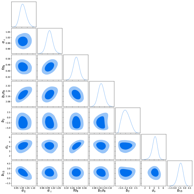
Figure 20: Full posterior distribution of the MCMC chain for the TNS model.

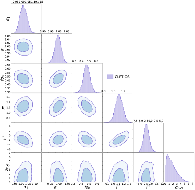
Figure 21: Full posterior distribution of the MCMC chain for the CLPT-GS model.

References

- Abolfathi et al. (2018) Abolfathi B., et al., 2018, The Astrophysical Journal Supplement Series, 235, 42
- Ahumada et al. (2019) Ahumada R., et al., 2019, arXiv:1912.02905 [astro-ph]
- Alam et al. (2017) Alam S., et al., 2017, Monthly Notices of the Royal Astronomical Society, 470, 2617
- Alam et al. (2020) Alam S., Someone et al. 2020, DR16 eBOSS ELG sample: Mock challenge paper, In preparation
- Albareti et al. (2017) Albareti F. D., et al., 2017, The Astrophysical Journal Supplement Series, 233, 25
- Alcock & Paczynski (1979) Alcock C., Paczynski B., 1979, Nature, 281, 358
- Amelie et al. (2020) Amelie Raichoor et al. 2020, The clustering of the SDSS-IV extended Baryon Oscillation Spectroscopic Survey ELG sample: Growth rate of structure measurement in configuration space between redshift 0.6 and 1.1., In preparation
- Anderson et al. (2014) Anderson L., et al., 2014, Monthly Notices of the Royal Astronomical Society, 439, 83
- Assassi et al. (2014) Assassi V., Baumann D., Green D., Zaldarriaga M., 2014, Journal of Cosmology and Astroparticle Physics, 08, 056
- Assassi et al. (2017) Assassi V., Simonović M., Zaldarriaga M., 2017, Journal of Cosmology and Astroparticle Physics, 11, 054
- Ata et al. (2018) Ata M., et al., 2018, Monthly Notices of the Royal Astronomical Society, 473, 4773
- Ávila et al. (2020) Ávila S., Someone et al. 2020, DR16 eBOSS ELG sample: constraining halo occupation models, In preparation
- Bautista et al. (2017) Bautista J. E., et al., 2017, Astronomy and Astrophysics, 603, A12
- Bautista et al. (2018) Bautista J. E., et al., 2018, The Astrophysical Journal, 863, 110
- Bel et al. (2019) Bel J., Pezzotta A., Carbone C., Sefusatti E., Guzzo L., 2019, Astronomy and Astrophysics, 622, A109
- Bernal et al. (2020) Bernal J. L., Smith T. L., Boddy K. K., Kamionkowski M., 2020, arXiv:2004.07263 [astro-ph]
- Beutler et al. (2011) Beutler F., et al., 2011, Monthly Notices of the Royal Astronomical Society, 416, 3017
- Beutler et al. (2012) Beutler F., et al., 2012, Monthly Notices of the Royal Astronomical Society, 423, 3430
- Beutler et al. (2017) Beutler F., et al., 2017, Monthly Notices of the Royal Astronomical Society, 466, 2242
- Bianchi & Percival (2017) Bianchi D., Percival W. J., 2017, Monthly Notices of the Royal Astronomical Society, 472, 1106
- Blake et al. (2011) Blake C., et al., 2011, Monthly Notices of the Royal Astronomical Society, 415, 2876
- Blanton et al. (2017) Blanton M. R., et al., 2017, The Astronomical Journal, 154, 28
- Burden et al. (2014) Burden A., Percival W. J., Manera M., Cuesta A. J., Vargas Magana M., Ho S., 2014, Monthly Notices of the Royal Astronomical Society, 445, 3152
- Burden et al. (2015) Burden A., Percival W. J., Howlett C., 2015, Monthly Notices of the Royal Astronomical Society, 453, 456
- Carlson et al. (2013) Carlson J., Reid B., White M., 2013, Monthly Notices of the Royal Astronomical Society, 429, 1674
- Carter et al. (2019) Carter P., Beutler F., Percival W. J., DeRose J., Wechsler R. H., Zhao C., 2019, arXiv:1906.03035 [astro-ph]
- Chan et al. (2012) Chan K. C., Scoccimarro R., Sheth R. K., 2012, Physical Review D, 85, 083509
- Chuang et al. (2015) Chuang C.-H., Kitaura F.-S., Prada F., Zhao C., Yepes G., 2015, Monthly Notices of the Royal Astronomical Society, 446, 2621
- Clifton et al. (2012) Clifton T., Ferreira P. G., Padilla A., Skordis C., 2012, Physics Reports, 513, 1
- Cole et al. (2005) Cole S., et al., 2005, Monthly Notices of the Royal Astronomical Society, 362, 505
- Collaboration et al. (2018a) Collaboration P., et al., 2018a, arXiv:1807.06205 [astro-ph]
- Collaboration et al. (2018b) Collaboration P., et al., 2018b, arXiv:1807.06209 [astro-ph]
- Dawson et al. (2013) Dawson K. S., et al., 2013, The Astronomical Journal, 145, 10
- Dawson et al. (2016) Dawson K. S., et al., 2016, The Astronomical Journal, 151, 44
- Eisenstein et al. (1998) Eisenstein D. J., Hu W., Tegmark M., 1998, The Astrophysical Journal Letters, 504, L57
- Eisenstein et al. (2005) Eisenstein D. J., et al., 2005, The Astrophysical Journal, 633, 560
- Eisenstein et al. (2011) Eisenstein D. J., et al., 2011, The Astronomical Journal, 142, 72
- Feldman et al. (1994) Feldman H. A., Kaiser N., Peacock J. A., 1994, The Astrophysical Journal, 426, 23
- Ferreira (2019) Ferreira P. G., 2019, Annual Review of Astronomy and Astrophysics, 57, 335
- Gil-Marín et al. (2020) Gil-Marín H., Bautista J., et al. 2020, DR16 eBOSS LRG analysis in Fourier space, In preparation
- Gil-Marín et al. (2018) Gil-Marín H., et al., 2018, Monthly Notices of the Royal Astronomical Society, 477, 1604
- Grieb et al. (2017) Grieb J. N., et al., 2017, Monthly Notices of the Royal Astronomical Society, 467, 2085
- Gunn et al. (2006) Gunn J. E., et al., 2006, The Astronomical Journal, 131, 2332
- Guzzo et al. (2008) Guzzo L., et al., 2008, Nature, 451, 541
- Hamilton (2000) Hamilton A. J. S., 2000, Monthly Notices of the Royal Astronomical Society, 312, 257
- Hartlap et al. (2007) Hartlap J., Simon P., Schneider P., 2007, Astronomy and Astrophysics, 464, 399
- Hearin et al. (2015) Hearin A. P., Watson D. F., van den Bosch F. C., 2015, Monthly Notices of the Royal Astronomical Society, 452, 1958
- Heitmann et al. (2019) Heitmann K., et al., 2019, The Astrophysical Journal Supplement Series, 245, 16
- Hou et al. (2018) Hou J., et al., 2018, Monthly Notices of the Royal Astronomical Society, 480, 2521
- Hou et al. (2020) Hou J., A. S., et al. 2020, DR16 eBOSS QSO analysis in configuration space, In preparation
- Howlett et al. (2015) Howlett C., Ross A. J., Samushia L., Percival W. J., Manera M., 2015, Monthly Notices of the Royal Astronomical Society, 449, 848
- Hutchinson et al. (2016) Hutchinson T. A., et al., 2016, The Astronomical Journal, 152, 205