\DeclareCaptionLabelFormat

andtable#1 #2 & Table 0

A Differential Game Theoretic Neural
Optimizer for Training Residual Networks

Guan-Horng Liu, Tianrong Chen, and Evangelos A. Theodorou
Autonomous Control and Decision Systems Laboratory
Georgia Institute of Technology,Atlanta, GA 30332
{ghliu,tianrong.chen,evangelos.theodorou}@gatech.edu
Abstract

Connections between Deep Neural Networks (DNNs) training and optimal control theory has attracted considerable attention as a principled tool of algorithmic design. Differential Dynamic Programming (DDP) neural optimizer [1] is a recently proposed method along this line. Despite its empirical success, the applicability has been limited to feedforward networks and whether such a trajectory-optimization inspired framework can be extended to modern architectures remains unclear. In this work, we derive a generalized DDP optimizer that accepts both residual connections and convolution layers. The resulting optimal control representation admits a game theoretic perspective, in which training residual networks can be interpreted as cooperative trajectory optimization on state-augmented dynamical systems. This Game Theoretic DDP (GT-DDP) optimizer enjoys the same theoretic connection in previous work, yet generates a much complex update rule that better leverages available information during network propagation. Evaluation on image classification datasets (e.g. MNIST and CIFAR100) shows an improvement in training convergence and variance reduction over existing methods. Our approach highlights the benefit gained from architecture-aware optimization.

1 Introduction

Attempts from different disciplines to provide a fundamental understanding of deep learning have advanced rapidly in recent years. Among those, interpretation of DNNs as discrete-time nonlinear dynamical systems, by viewing each layer as a distinct time step, has received tremendous focus as it enables rich analysis ranging from numerical equations [2], mean-field theory [3], to physics [4, 5, 6]. For instance, interpretation of residual networks as a discretization of ordinary differential equations (ODEs) [7] provides theoretical reasoning on its optimization landscape [8]. It also inspires new architecture that inherits numerical stability [9, 10, 11] and differential limit [12, 13].

Development of practical optimization methods, however, remains relatively limited. This is primarily because classical approach to optimize dynamical systems relies on the optimal control theory, which typically considers systems with neither the dimensionality nor parameterization as high as DNNs. Such a difficulty limits its application, despite showing promising convergence and robustness in trajectory optimization [14], to mostly theoretical interpretation of DNNs training [15, 16]. The algorithmic progress has been restricted to either specific network class (e.g. discrete weight [17]) or training procedure (e.g. hyper-parameter adaptation [18] or computational acceleration [19, 20]), until the recently proposed Differential Dynamic Programming (DDP) optimizer [1].

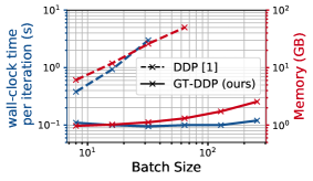
DDP is a second-order optimizer built upon a formal connection between trajectory optimization and training feedforward networks, and from such it suggests existing training algorithms can be lifted to embrace the dynamic programming principle, resulting in superior parameter updates with layer-wise feedback policies. However, DDP is an architecture-dependent optimizer, in that the feedback policies need to be derived on a per architecture basis. This raise questions of its flexibility and scalability to training modern architectures such as residual networks [21], since the existing formulation scales exponentially with the batch size (see Fig. 1).
Refer to caption
Figure 1: Comparison on MNIST.

In this work, we present a game-theoretic extension to the DDP optimizer (GT-DDP) which arises naturally from the optimal control representation of residual networks. GT-DDP treats each layer as a decision maker in a multi-stage coalition game connected through network propagation. This leads to much complex feedback policies as information is allowed to exchanged between layers. Despite the increasing computation, we leverage efficient approximations which enable GT-DDP to run on a faster wall-clock yet with less memory (see Fig. 1). On the theoretical side, we extend previous analysis for feedforward networks to arbitrary architecture (Proposition 4), and derive game-theoretic integration for existing second-order optimizers (Theorem 3 and Corollary 7). GT-DDP shows an overall improvement on image classification dataset.

There has been a rising interest in game-theoretic analysis since the landmark Generative Adversarial Network [22]. By framing networks into a two-player competing game, prevalent efforts have been spent on studying its convergence dynamics [23] and effective optimizers to find stable saddle points [24, 25], Notably, our layer-as-player formulation has appeared in Balduzzi [26] to study the signal communication implied in the Back-propagation, yet without any practical algorithm being made. On the other hand, the cooperative game framework has been used to discover neuron contribution in representation learning and network pruning [27, 28], which are of independent interest for this work.

The paper is organized as follows. We first review the connection between optimal control and DNNs training in Sec. 2. Extending such framework to residual networks is then given in Sec. 3, with GT-DDP demonstrated in Sec. 4. We provide empirical results and discussion in Sec. 5 and 6.

footnotetext: Notation: t𝑡t will always be denoted the time step of dynamics, or equivalently the layer’s index. Given a time-dependent function t(𝒙t,𝒖t):𝕏×𝕌:subscript𝑡subscript𝒙𝑡subscript𝒖𝑡maps-to𝕏𝕌\mathcal{F}_{t}({\bm{x}}_{t},{\bm{u}}_{t}):\mathbb{X}\times\mathbb{U}\mapsto\mathbb{R}, we will denote and sometimes abbreviate it Jacobian, Hessian, and mixed partial derivative respectively as 𝒙tt𝒙tsubscriptsubscript𝒙𝑡subscript𝑡subscriptsuperscript𝑡𝒙\nabla_{{\bm{x}}_{t}}\mathcal{F}_{t}\equiv\mathcal{F}^{t}_{{\bm{x}}}, 𝒙t2t𝒙𝒙tsuperscriptsubscriptsubscript𝒙𝑡2subscript𝑡subscriptsuperscript𝑡𝒙𝒙\nabla_{{\bm{x}}_{t}}^{2}\mathcal{F}_{t}\equiv\mathcal{F}^{t}_{{\bm{x}}{\bm{x}}}, and 𝒙t𝒖tt𝒙𝒖tsubscriptsubscript𝒙𝑡subscriptsubscript𝒖𝑡subscript𝑡subscriptsuperscript𝑡𝒙𝒖\nabla_{{\bm{x}}_{t}}\nabla_{{\bm{u}}_{t}}\mathcal{F}_{t}\equiv\mathcal{F}^{t}_{{\bm{x}}{\bm{u}}}.

2 Preliminaries

2.1 Optimal Control Formulation of Training DNNs

Classical optimal control problem (OCP) in discrete time considers the following programming:

min𝒖¯J(𝒖¯;𝒙0):=[ϕ(𝒙T)+t=0T1t(𝒙t,𝒖t)]s.t. 𝒙t+1=ft(𝒙t,𝒖t) ,formulae-sequenceassignsubscript¯𝒖𝐽¯𝒖subscript𝒙0delimited-[]italic-ϕsubscript𝒙𝑇superscriptsubscript𝑡0𝑇1subscript𝑡subscript𝒙𝑡subscript𝒖𝑡s.t. subscript𝒙𝑡1subscript𝑓𝑡subscript𝒙𝑡subscript𝒖𝑡 ,\min_{{\bar{{\bm{u}}}}}J(\bar{{\bm{u}}};{\bm{x}}_{0}):=\left[\phi({\bm{x}}_{T})+\sum_{t=0}^{T-1}\ell_{t}({\bm{x}}_{t},{\bm{u}}_{t})\right]\quad\text{s.t. }{\bm{x}}_{t+1}=f_{t}({\bm{x}}_{t},{\bm{u}}_{t}){\text{ ,}} (1)

where 𝒙tntsubscript𝒙𝑡superscriptsubscript𝑛𝑡{\bm{x}}_{t}\in\mathbb{R}^{n_{t}} and 𝒖tmtsubscript𝒖𝑡superscriptsubscript𝑚𝑡{\bm{u}}_{t}\in\mathbb{R}^{m_{t}} represent the state and control at each time step t{0,,T}𝑡0𝑇t\in\{0,\cdots,T\}. ftsubscript𝑓𝑡f_{t}, tsubscript𝑡\ell_{t} and ϕitalic-ϕ\phi respectively denote the dynamics, intermediate cost and terminal cost. The control trajectory is denoted as 𝒖¯{𝒖t}t=0T1¯𝒖superscriptsubscriptsubscript𝒖𝑡𝑡0𝑇1{\bar{{\bm{u}}}}\triangleq\{{\bm{u}}_{t}\}_{t=0}^{T-1}. Eq. (1) can be interpreted as the training objective of DNNs by treating 𝒙tsubscript𝒙𝑡{\bm{x}}_{t} and 𝒖tsubscript𝒖𝑡{\bm{u}}_{t} as the vectorized activation map (𝒙0subscript𝒙0{\bm{x}}_{0} and 𝒙Tsubscript𝒙𝑇{\bm{x}}_{T} being input image and prediction vector) and weight at each layer t𝑡t. ftsubscript𝑓𝑡f_{t} stands as the compositional module propagating the activation vector, e.g. an affine transformation followed by an element-wise activation in a feedforward network. tsubscript𝑡\ell_{t} and ϕitalic-ϕ\phi denote the per-layer regularization (e.g. weight decay) and terminal loss (e.g. cross-entropy).

Following these notations, the gradient descent (GD) update at iteration k𝑘k can be written as 𝒖¯(k+1)=𝒖¯(k)+δ𝒖¯=𝒖¯(k)η𝒖¯Jsuperscript¯𝒖𝑘1superscript¯𝒖𝑘𝛿superscript¯𝒖superscript¯𝒖𝑘𝜂subscript¯𝒖𝐽{\bar{{\bm{u}}}}^{(k+1)}={\bar{{\bm{u}}}}^{(k)}+\delta{\bar{{\bm{u}}}}^{*}={\bar{{\bm{u}}}}^{(k)}-\eta\nabla_{{\bar{{\bm{u}}}}}J, where η𝜂\eta is the learning rate. We can further break down the update for the full network to each layer, i.e. δ𝒖¯{δ𝒖t}t=0T1𝛿¯𝒖superscriptsubscript𝛿subscript𝒖𝑡𝑡0𝑇1\delta{\bar{{\bm{u}}}}\triangleq\{\delta{\bm{u}}_{t}\}_{t=0}^{T-1}, computed backward by

δ𝒖t𝛿superscriptsubscript𝒖𝑡\displaystyle{\delta{\bm{u}}}_{t}^{*} =argminδ𝒖tmt{Jt+𝒖tJt𝖳δ𝒖t+12δ𝒖t𝖳(1η𝑰t)δ𝒖t} ,absentsubscriptargmin𝛿subscript𝒖𝑡superscriptsubscript𝑚𝑡subscript𝐽𝑡subscriptsubscript𝒖𝑡superscriptsubscript𝐽𝑡𝖳𝛿subscript𝒖𝑡12𝛿superscriptsubscript𝒖𝑡𝖳1𝜂subscript𝑰𝑡𝛿subscript𝒖𝑡 ,\displaystyle=\operatorname*{arg\,min}_{{\delta{\bm{u}}}_{t}\in\mathbb{R}^{m_{t}}}\{J_{t}+\nabla_{{\bm{u}}_{t}}J_{t}^{\mathsf{T}}{\delta{\bm{u}}}_{t}+\textstyle\frac{1}{2}{\delta{\bm{u}}}_{t}^{\mathsf{T}}(\textstyle\frac{1}{\eta}{\bm{I}}_{t}){\delta{\bm{u}}}_{t}\}{\text{ ,}} (2)
where Jt(𝒙t,𝒖t)where subscript𝐽𝑡subscript𝒙𝑡subscript𝒖𝑡\displaystyle\text{where }J_{t}({\bm{x}}_{t},{\bm{u}}_{t}) t(𝒖t)+Jt+1(ft(𝒙t,𝒖t),𝒖t+1) ,JT(𝒙T)ϕ(𝒙T)formulae-sequenceabsentsubscript𝑡subscript𝒖𝑡subscript𝐽𝑡1subscript𝑓𝑡subscript𝒙𝑡subscript𝒖𝑡subscript𝒖𝑡1 ,subscript𝐽𝑇subscript𝒙𝑇italic-ϕsubscript𝒙𝑇\displaystyle\triangleq\ell_{t}({\bm{u}}_{t})+J_{t+1}(f_{t}({\bm{x}}_{t},{\bm{u}}_{t}),{\bm{u}}_{t+1}){\text{ ,}}\quad J_{T}({\bm{x}}_{T})\triangleq\phi({\bm{x}}_{T}) (3)

is the per-stage objective111 We drop 𝒙tsubscript𝒙𝑡{\bm{x}}_{t} in all t()subscript𝑡\ell_{t}(\cdot) hereafter as the layer-wise regularization typically involves network weight alone. at layer t𝑡t. It can be readily verified that 𝒙tJtsubscriptsubscript𝒙𝑡subscript𝐽𝑡\nabla_{{\bm{x}}_{t}}J_{t} gives the exact Back-propagation dynamics. Eq. (2) follows the standard optimization interpretation in which GD minimizes the second-order Taylor expansion of Jtsubscript𝐽𝑡J_{t} with its Hessian 𝒖t2Jtsuperscriptsubscriptsubscript𝒖𝑡2subscript𝐽𝑡\nabla_{{\bm{u}}_{t}}^{2}J_{t} replaced by 1η𝑰t1𝜂subscript𝑰𝑡\frac{1}{\eta}{\bm{I}}_{t}, i.e. spherical curvature. In a similar vein, adaptive first-order methods, such as RMSprop and Adam, approximate 𝒖t2Jtsuperscriptsubscriptsubscript𝒖𝑡2subscript𝐽𝑡\nabla_{{\bm{u}}_{t}}^{2}J_{t} by diagonal matrices with the leading entries adapting to the second-moment statistics in each coordinate. Second-order optimizers like KFAC [29, 30] and EKFAC [31] compute much complex non-diagonal curvature matrices with Gauss-Newton approximation, i.e. 𝒖t2JtJ𝒖tJ𝒖t𝖳superscriptsubscriptsubscript𝒖𝑡2subscript𝐽𝑡subscriptsuperscript𝐽𝑡𝒖superscriptsubscriptsuperscript𝐽𝑡𝒖𝖳\nabla_{{\bm{u}}_{t}}^{2}J_{t}\approx J^{t}_{\bm{u}}{J^{t}_{\bm{u}}}^{\mathsf{T}}.

Algorithm 1 DDP Neural Optimizer (at iteration k𝑘k)
1:  Input: forward pass {𝒙t}t=0Tsuperscriptsubscriptsubscript𝒙𝑡𝑡0𝑇\{{{\bm{x}}}_{t}\}_{t=0}^{T} with weights 𝒖¯(k)superscript¯𝒖𝑘\bar{{\bm{u}}}^{(k)}
2:  Set V𝒙T=𝒙ϕsuperscriptsubscript𝑉𝒙𝑇subscript𝒙italic-ϕV_{\bm{x}}^{T}=\nabla_{\bm{x}}\phi and V𝒙𝒙T=𝒙2ϕsuperscriptsubscript𝑉𝒙𝒙𝑇subscriptsuperscript2𝒙italic-ϕV_{{\bm{x}}{\bm{x}}}^{T}=\nabla^{2}_{{\bm{x}}}\phi
3:  for t=T1𝑡𝑇1t=T-1 to 00 do
4:     Compute derivatives of Qtsubscript𝑄𝑡Q_{t} with V𝒙t+1superscriptsubscript𝑉𝒙𝑡1V_{{\bm{x}}}^{t+1}, V𝒙𝒙t+1superscriptsubscript𝑉𝒙𝒙𝑡1V_{{\bm{x}}{\bm{x}}}^{t+1}
5:     Compute 𝐤tsubscript𝐤𝑡{\mathbf{k}_{t}}, 𝐊tsubscript𝐊𝑡{\mathbf{K}_{t}}, V𝒙tsuperscriptsubscript𝑉𝒙𝑡V_{{\bm{x}}}^{t} and V𝒙𝒙tsuperscriptsubscript𝑉𝒙𝒙𝑡V_{{\bm{x}}{\bm{x}}}^{t}
6:  end for
7:  Set 𝒙^0=𝒙0subscript^𝒙0subscript𝒙0\hat{{\bm{x}}}_{0}={{\bm{x}}}_{0}
8:  for t=0𝑡0t=0 to T1𝑇1T-1 do
9:     𝒖^t=𝒖t(k)+𝐤t+𝐊tδ𝒙t,   (δ𝒙t=𝒙^t𝒙t)subscript^𝒖𝑡superscriptsubscript𝒖𝑡𝑘subscript𝐤𝑡subscript𝐊𝑡𝛿subscript𝒙𝑡   𝛿subscript𝒙𝑡subscript^𝒙𝑡subscript𝒙𝑡\hat{{\bm{u}}}_{t}={{\bm{u}}}_{t}^{(k)}+{\mathbf{k}_{t}}+{\mathbf{K}_{t}}{\delta{\bm{x}}}_{t},\text{ }\text{ }\text{ }({\delta{\bm{x}}}_{t}=\hat{{\bm{x}}}_{t}-{{\bm{x}}}_{t})
10:     𝒙^t+1=ft(𝒙^t,𝒖^t)subscript^𝒙𝑡1subscript𝑓𝑡subscript^𝒙𝑡subscript^𝒖𝑡\hat{{\bm{x}}}_{t+1}=f_{t}(\hat{{\bm{x}}}_{t},\hat{{\bm{u}}}_{t})
11:  end for
12:  𝒖¯(k+1){𝒖^t}t=0T1superscript¯𝒖𝑘1superscriptsubscriptsubscript^𝒖𝑡𝑡0𝑇1{\bar{{\bm{u}}}}^{(k+1)}\leftarrow\{\hat{{\bm{u}}}_{t}\}_{t=0}^{T-1}
Refer to caption
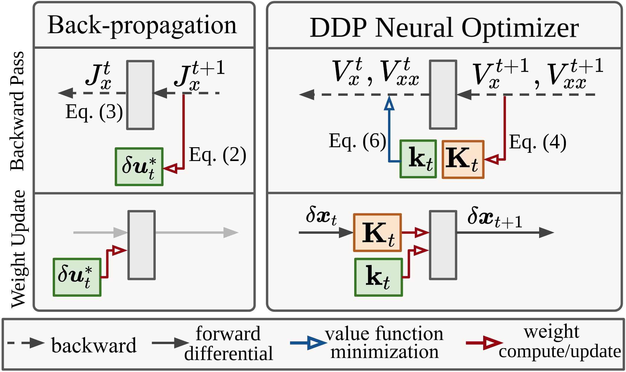
Figure 2: Comparison of computational graphs in feedforward networks.

2.2 Differential Dynamic Programming Neural Optimizer

Differential Dynamic Programming (DDP) is a second-order trajectory optimization algorithm that solves the same programming in Eq. (1). Instead of searching updates from mtsuperscriptsubscript𝑚𝑡\mathbb{R}^{m_{t}}, at each decision stage DDP aims at finding a locally-optimal feedback policy, i.e. δ𝒖t(δ𝒙t)Γδ𝒙t𝛿subscript𝒖𝑡𝛿subscript𝒙𝑡subscriptΓ𝛿subscript𝒙𝑡{\delta{\bm{u}}}_{t}({\delta{\bm{x}}}_{t})\in\Gamma_{{\delta{\bm{x}}}_{t}}, where Γδ𝒙t={𝐛t+𝐀tδ𝒙t:𝐛tmt,𝐀tmt×nt}subscriptΓ𝛿subscript𝒙𝑡conditional-setsubscript𝐛𝑡subscript𝐀𝑡𝛿subscript𝒙𝑡formulae-sequencesubscript𝐛𝑡superscriptsubscript𝑚𝑡subscript𝐀𝑡superscriptsubscript𝑚𝑡subscript𝑛𝑡\Gamma_{{\delta{\bm{x}}}_{t}}=\{\mathbf{b}_{t}+\mathbf{A}_{t}{\delta{\bm{x}}}_{t}:\mathbf{b}_{t}\in\mathbb{R}^{m_{t}},\mathbf{A}_{t}\in\mathbb{R}^{{m_{t}}\times{n_{t}}}\} denotes all possible affine mappings from the state differential δ𝒙t𝛿subscript𝒙𝑡{\delta{\bm{x}}}_{t}. The resulting per-stage updates can also be computed backward:

δ𝒖t(δ𝒙t)=argminδ𝒖tΓδ𝒙t𝛿superscriptsubscript𝒖𝑡𝛿subscript𝒙𝑡subscriptargmin𝛿subscript𝒖𝑡subscriptΓ𝛿subscript𝒙𝑡\displaystyle{\delta{\bm{u}}}_{t}^{*}({\delta{\bm{x}}}_{t})=\operatorname*{arg\,min}_{{\delta{\bm{u}}}_{t}\in\Gamma_{{\delta{\bm{x}}}_{t}}} {Qt+12[𝟏δ𝒙tδ𝒖t]𝖳[𝟎Q𝒙t𝖳Q𝒖t𝖳Q𝒙tQ𝒙𝒙tQ𝒙𝒖tQ𝒖tQ𝒖𝒙tQ𝒖𝒖t][𝟏δ𝒙tδ𝒖t]} ,subscript𝑄𝑡12superscriptdelimited-[]1𝛿subscript𝒙𝑡𝛿subscript𝒖𝑡𝖳delimited-[]0superscriptsubscriptsuperscript𝑄𝑡𝒙𝖳superscriptsubscriptsuperscript𝑄𝑡𝒖𝖳subscriptsuperscript𝑄𝑡𝒙subscriptsuperscript𝑄𝑡𝒙𝒙subscriptsuperscript𝑄𝑡𝒙𝒖subscriptsuperscript𝑄𝑡𝒖subscriptsuperscript𝑄𝑡𝒖𝒙subscriptsuperscript𝑄𝑡𝒖𝒖delimited-[]1𝛿subscript𝒙𝑡𝛿subscript𝒖𝑡 ,\displaystyle\{Q_{t}+\frac{1}{2}\left[\begin{array}[]{c}{\mathbf{1}}\\ {{\delta{\bm{x}}}_{t}}\\ {{\delta{\bm{u}}}_{t}}\end{array}\right]^{{\mathsf{T}}}\left[\begin{array}[]{ccc}{\mathbf{0}}&{{Q^{t}_{{\bm{x}}}}^{\mathsf{T}}}&{{Q^{t}_{{\bm{u}}}}^{\mathsf{T}}}\\ {{Q^{t}_{{\bm{x}}}}}&{{Q^{t}_{{\bm{x}}{\bm{x}}}}}&{{Q^{t}_{{\bm{x}}{\bm{u}}}}}\\ {{Q^{t}_{{\bm{u}}}}}&{{Q^{t}_{{\bm{u}}{\bm{x}}}}}&{{Q^{t}_{{\bm{u}}{\bm{u}}}}}\end{array}\right]\left[\begin{array}[]{c}{\mathbf{1}}\\ {{\delta{\bm{x}}}_{t}}\\ {{\delta{\bm{u}}}_{t}}\end{array}\right]\}{\text{ ,}} (13)
where Vt(𝒙t)min𝒖tΓ𝒙twhere subscript𝑉𝑡subscript𝒙𝑡subscriptsubscript𝒖𝑡subscriptΓsubscript𝒙𝑡\displaystyle\text{where }V_{t}({\bm{x}}_{t})\triangleq\min_{{\bm{u}}_{t}\in\Gamma_{{\bm{x}}_{t}}} t(𝒖t)+Vt+1(ft(𝒙t,𝒖t))Qt(𝒙t,𝒖t)Qt ,VT(𝒙T)ϕ(𝒙T)subscriptsubscript𝑡subscript𝒖𝑡subscript𝑉𝑡1subscript𝑓𝑡subscript𝒙𝑡subscript𝒖𝑡subscript𝑄𝑡subscript𝒙𝑡subscript𝒖𝑡subscript𝑄𝑡 ,subscript𝑉𝑇subscript𝒙𝑇italic-ϕsubscript𝒙𝑇\displaystyle\underbrace{\ell_{t}({\bm{u}}_{t})+V_{t+1}(f_{t}({\bm{x}}_{t},{\bm{u}}_{t}))}_{Q_{t}({\bm{x}}_{t},{\bm{u}}_{t})\equiv Q_{t}}{\text{ ,}}\quad V_{T}({\bm{x}}_{T})\triangleq\phi({\bm{x}}_{T}) (14)

is the value function that summarizes the objective value when all the afterward stages, i.e. Qstsubscript𝑄𝑠𝑡Q_{s\geq t}, are minimized. Hereafter we will denote the quadratic expansion in Eq. (13) as δQt(δ𝒙t,δ𝒖t)𝛿subscript𝑄𝑡𝛿subscript𝒙𝑡𝛿subscript𝒖𝑡\delta Q_{t}({\delta{\bm{x}}}_{t},{\delta{\bm{u}}}_{t}). Qtsubscript𝑄𝑡Q_{t} will be referred to the Bellman objective, as Eq. (14) is well-known as the Bellman equation [32].

The analytic solution to Eq. (13) is given by δ𝒖t(δ𝒙t)=𝐤t+𝐊tδ𝒙t𝛿subscriptsuperscript𝒖𝑡𝛿subscript𝒙𝑡subscript𝐤𝑡subscript𝐊𝑡𝛿subscript𝒙𝑡{\delta{\bm{u}}}^{*}_{t}({\delta{\bm{x}}}_{t})={\mathbf{k}_{t}}+{\mathbf{K}_{t}}{\delta{\bm{x}}}_{t}, where 𝐤t(Q𝒖𝒖t)1Q𝒖tsubscript𝐤𝑡superscriptsubscriptsuperscript𝑄𝑡𝒖𝒖1subscriptsuperscript𝑄𝑡𝒖{\mathbf{k}_{t}}\triangleq-({Q^{t}_{{\bm{u}}{\bm{u}}}})^{-1}{Q^{t}_{{\bm{u}}}} and 𝐊t(Q𝒖𝒖t)1Q𝒖𝒙tsubscript𝐊𝑡superscriptsubscriptsuperscript𝑄𝑡𝒖𝒖1subscriptsuperscript𝑄𝑡𝒖𝒙{\mathbf{K}_{t}}\triangleq-({Q^{t}_{{\bm{u}}{\bm{u}}}})^{-1}{Q^{t}_{{\bm{u}}{\bm{x}}}} are the locally optimal open and feedback gains. From the chain rule, evaluating the derivatives of Qtsubscript𝑄𝑡Q_{t} in Eq. (13) requires one to compute V𝒙t+1subscriptsuperscript𝑉𝑡1𝒙V^{t+1}_{{\bm{x}}} and V𝒙𝒙t+1subscriptsuperscript𝑉𝑡1𝒙𝒙V^{t+1}_{{\bm{x}}{\bm{x}}}. These quantities can be obtained by simply substituting δ𝒖t(δ𝒙t)𝛿subscriptsuperscript𝒖𝑡𝛿subscript𝒙𝑡{\delta{\bm{u}}}^{*}_{t}({\delta{\bm{x}}}_{t}) to Eq. (14) at each stage:

V𝒙t=𝒙t{Qt+δQt(δ𝒙t,δ𝒖t(δ𝒙t))}=Q𝒙t+Q𝒙𝒖t𝐤t ,V𝒙𝒙t=𝒙t2{Qt+δQt(δ𝒙t,δ𝒖t(δ𝒙t))}=Q𝒙𝒙t+Q𝒙𝒖t𝐊t .superscriptsubscript𝑉𝒙𝑡subscriptsubscript𝒙𝑡subscript𝑄𝑡𝛿subscript𝑄𝑡𝛿subscript𝒙𝑡𝛿subscriptsuperscript𝒖𝑡𝛿subscript𝒙𝑡subscriptsuperscript𝑄𝑡𝒙subscriptsuperscript𝑄𝑡𝒙𝒖subscript𝐤𝑡 ,superscriptsubscript𝑉𝒙𝒙𝑡superscriptsubscriptsubscript𝒙𝑡2subscript𝑄𝑡𝛿subscript𝑄𝑡𝛿subscript𝒙𝑡𝛿subscriptsuperscript𝒖𝑡𝛿subscript𝒙𝑡subscriptsuperscript𝑄𝑡𝒙𝒙subscriptsuperscript𝑄𝑡𝒙𝒖subscript𝐊𝑡 .\displaystyle\begin{split}V_{{\bm{x}}}^{t}&=\nabla_{{\bm{x}}_{t}}\{Q_{t}+\delta Q_{t}({\delta{\bm{x}}}_{t},{\delta{\bm{u}}}^{*}_{t}({\delta{\bm{x}}}_{t}))\}={Q^{t}_{{\bm{x}}}}+{Q^{t}_{{\bm{x}}{\bm{u}}}}{\mathbf{k}_{t}}{\text{ ,}}\\ V_{{\bm{x}}{\bm{x}}}^{t}&=\nabla_{{\bm{x}}_{t}}^{2}\{Q_{t}+\delta Q_{t}({\delta{\bm{x}}}_{t},{\delta{\bm{u}}}^{*}_{t}({\delta{\bm{x}}}_{t}))\}={Q^{t}_{{\bm{x}}{\bm{x}}}}+{Q^{t}_{{\bm{x}}{\bm{u}}}}{\mathbf{K}_{t}}{\text{ .}}\end{split} (15)

It is obvious that Eq. (13, 14) resemble Eq. (2, 3) in several ways. Both classes of optimizer perform quadratic approximation of the stage-wise objective, except DDP also expands the objective wrt δ𝒙t𝛿subscript𝒙𝑡{\delta{\bm{x}}}_{t}, which requires computing the mixed partial derivatives Q𝒖𝒙tsubscriptsuperscript𝑄𝑡𝒖𝒙{Q^{t}_{{\bm{u}}{\bm{x}}}}. The theoretical connection between these two approaches for feedforward networks has been made formally in Liu et al. [1].

Proposition 1 ([1]).

When Q𝐮𝐱t=𝟎superscriptsubscript𝑄𝐮𝐱𝑡0Q_{{\bm{u}}{\bm{x}}}^{t}=\mathbf{0} at all stages, the first-order derivative of the value function collapses to the Back-propagation gradient in feedforward networks, i.e. V𝐱t=J𝐱tsubscriptsuperscript𝑉𝑡𝐱subscriptsuperscript𝐽𝑡𝐱V^{t}_{{\bm{x}}}=J^{t}_{{\bm{x}}}. In this case, DDP computes the same update in stage-wise Newton222 Stage-wise Newton preconditions the gradient by the block-wise inverse Hessian at each layer. : δ𝐮t(δ𝐱t)=(J𝐮𝐮t)1J𝐮t𝛿subscriptsuperscript𝐮𝑡𝛿subscript𝐱𝑡superscriptsubscriptsuperscript𝐽𝑡𝐮𝐮1subscriptsuperscript𝐽𝑡𝐮{\delta{\bm{u}}}^{*}_{t}({\delta{\bm{x}}}_{t})=-(J^{t}_{{\bm{u}}{\bm{u}}})^{{-1}}J^{t}_{{\bm{u}}}. If we further assume Q𝐮𝐮t=1η𝐈tsuperscriptsubscript𝑄𝐮𝐮𝑡1𝜂subscript𝐈𝑡{Q_{{\bm{u}}{\bm{u}}}^{t}}=\frac{1}{\eta}{\bm{I}}_{t}, then DDP degenerates to the Back-propagation with gradient descent.

Proposition 1 suggests that by setting Q𝒖𝒙t=𝟎subscriptsuperscript𝑄𝑡𝒖𝒙0{Q^{t}_{{\bm{u}}{\bm{x}}}}=\mathbf{0} and choosing a proper Q𝒖𝒖tsubscriptsuperscript𝑄𝑡𝒖𝒖{Q^{t}_{{\bm{u}}{\bm{u}}}}, we can recover existing optimizers from DDP. Meanwhile, existing methods can be extended to accept DDP framework by computing Q𝒖𝒙tsubscriptsuperscript𝑄𝑡𝒖𝒙{Q^{t}_{{\bm{u}}{\bm{x}}}}. The resulting layer-wise feedback policies generate weight update with additional forward pass (lines 777-111111 in Alg. 1), in which the state differential is computed. We summarize the backward pass and weight update procedure of the DDP optimizer in Alg. 1 and Fig. 2.

3 Optimal Control Representation for Residual Networks

In this section, we extend the Bellman optimization framework to networks consist of residual paths. Despite that in the Back-propagation this simply involves merging additional gradient flow from the shortcut, its optimal control representation is much complex when second-order information and Bellman minimization are involved. We leave the complete derivation in the Appendix A.

3.1 Residual Connection as State-Augmented Dynamics

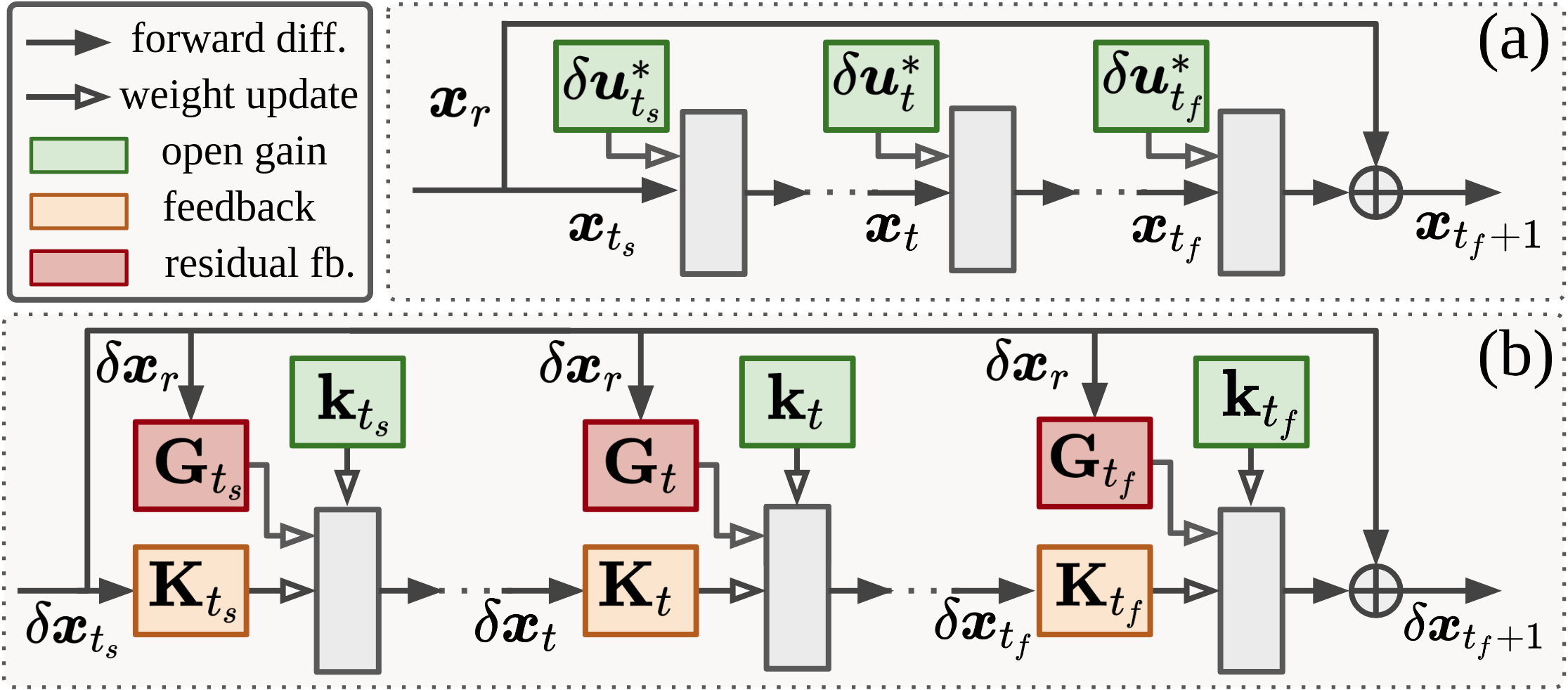
Consider the residual network in Fig. 3a. Let us denote 𝒙rsubscript𝒙𝑟{\bm{x}}_{r} as the residual state shortcutting from the layer tssubscript𝑡𝑠t_{s} to tfsubscript𝑡𝑓t_{f}, so that the output is merged by 𝒙tf+1=𝒙r+ftf(𝒙tf,𝒖tf)subscript𝒙subscript𝑡𝑓1subscript𝒙𝑟subscript𝑓subscript𝑡𝑓subscript𝒙subscript𝑡𝑓subscript𝒖subscript𝑡𝑓{\bm{x}}_{t_{f}+1}={\bm{x}}_{r}+f_{t_{f}}({\bm{x}}_{t_{f}},{\bm{u}}_{t_{f}}). The Bellman equation along the residual path is given by

Vts(𝒙ts)=min𝒖t[ts,tf]ts(𝒖ts)++tf(𝒖tf)+Vtf+1(𝒙r+(ftffts)(𝒙ts)) ,subscript𝑉subscript𝑡𝑠subscript𝒙subscript𝑡𝑠subscriptsubscript𝒖𝑡subscript𝑡𝑠subscript𝑡𝑓subscriptsubscript𝑡𝑠subscript𝒖subscript𝑡𝑠subscriptsubscript𝑡𝑓subscript𝒖subscript𝑡𝑓subscript𝑉subscript𝑡𝑓1subscript𝒙𝑟subscript𝑓subscript𝑡𝑓subscript𝑓subscript𝑡𝑠subscript𝒙subscript𝑡𝑠 ,\displaystyle V_{t_{s}}({\bm{x}}_{t_{s}})=\textstyle\min_{{\bm{u}}_{t\in[t_{s},t_{f}]}}\ell_{t_{s}}({\bm{u}}_{t_{s}})+\cdots+\ell_{t_{f}}({\bm{u}}_{t_{f}})+V_{t_{f}+1}({{\bm{x}}_{r}}+(f_{t_{f}}\circ\cdots\circ f_{t_{s}})({\bm{x}}_{t_{s}})){\text{ ,}} (16)

which can be decomposed into the following minimization and solve recursively from tfsubscript𝑡𝑓t_{f}:

Vt(𝒙r,𝒙t)=min𝒖tQt(𝒙r,𝒙t,𝒖t):={t(𝒖t)+Vt+1(𝒙r+ft(𝒙t,𝒖t)) ,t=tfsubscript𝑉𝑡subscript𝒙𝑟subscript𝒙𝑡subscriptsubscript𝒖𝑡subscript𝑄𝑡subscript𝒙𝑟subscript𝒙𝑡subscript𝒖𝑡assigncasesmissing-subexpressionsubscript𝑡subscript𝒖𝑡subscript𝑉𝑡1subscript𝒙𝑟subscript𝑓𝑡subscript𝒙𝑡subscript𝒖𝑡 ,𝑡subscript𝑡𝑓\displaystyle\raisebox{-10.53333pt}[0.0pt][0.0pt]{\leavevmode\hbox{\set@color$V_{t}({{\bm{x}}_{r}},{\bm{x}}_{t})=\textstyle\min_{{\bm{u}}_{t}}Q_{t}({{\bm{x}}_{r}},{\bm{x}}_{t},{\bm{u}}_{t}):=\left\{\begin{array}[]{@{}c@{}}\vphantom{\ell_{t}({\bm{u}}_{t})+V_{t+1}({{\bm{x}}_{r}}+f_{t}({\bm{x}}_{t},{\bm{u}}_{t})){\text{ ,}}\quad t=t_{f}}\\ \vphantom{\ell_{t}({\bm{u}}_{t})+V_{t+1}({{\bm{x}}_{r}},f_{t}({\bm{x}}_{t},{\bm{u}}_{t})){\text{ ,}}\quad t\in(t_{s},t_{f})}\end{array}\right.\kern-1.2pt$}}\ell_{t}({\bm{u}}_{t})+V_{t+1}({{\bm{x}}_{r}}+f_{t}({\bm{x}}_{t},{\bm{u}}_{t})){\text{ ,}}\quad t=t_{f}\quad (17c)
t(𝒖t)+Vt+1(𝒙r,ft(𝒙t,𝒖t)) ,t(ts,tf)subscript𝑡subscript𝒖𝑡subscript𝑉𝑡1subscript𝒙𝑟subscript𝑓𝑡subscript𝒙𝑡subscript𝒖𝑡 ,𝑡subscript𝑡𝑠subscript𝑡𝑓\displaystyle\ell_{t}({\bm{u}}_{t})+V_{t+1}({{\bm{x}}_{r}},f_{t}({\bm{x}}_{t},{\bm{u}}_{t})){\text{ ,}}\quad t\in(t_{s},t_{f}) (17d)
Vts(𝒙ts)=min𝒖tsQts(𝒙ts,𝒖ts):=ts(𝒖ts)+Vts+1(𝒙ts,fts(𝒙ts,𝒖ts))subscript𝑉subscript𝑡𝑠subscript𝒙subscript𝑡𝑠subscriptsubscript𝒖subscript𝑡𝑠subscript𝑄subscript𝑡𝑠subscript𝒙subscript𝑡𝑠subscript𝒖subscript𝑡𝑠assignsubscriptsubscript𝑡𝑠subscript𝒖subscript𝑡𝑠subscript𝑉subscript𝑡𝑠1subscript𝒙subscript𝑡𝑠subscript𝑓subscript𝑡𝑠subscript𝒙subscript𝑡𝑠subscript𝒖subscript𝑡𝑠\displaystyle V_{t_{s}}({\bm{x}}_{t_{s}})=\textstyle\min_{{\bm{u}}_{t_{s}}}Q_{t_{s}}({\bm{x}}_{t_{s}},{\bm{u}}_{t_{s}}):=\ell_{t_{s}}({\bm{u}}_{t_{s}})+V_{t_{s}+1}({\bm{x}}_{t_{s}},f_{t_{s}}({\bm{x}}_{t_{s}},{\bm{u}}_{t_{s}}))\qquad\qquad (17e)

Eq. (17) suggests the value functions of layers parallel to the shortcut depend not only on its own state 𝒙tsubscript𝒙𝑡{\bm{x}}_{t} but also the residual 𝒙rsubscript𝒙𝑟{\bm{x}}_{r}. This is better explained from the game theoretic viewpoint. As 𝒙rsubscript𝒙𝑟{\bm{x}}_{r} affects the payoff obtained during t[ts,tf]𝑡subscript𝑡𝑠subscript𝑡𝑓t\in[t_{s},t_{f}] through the addition at tf+1subscript𝑡𝑓1t_{f}+1, it shall contribute to decisions made at these stages. Notice that we can rewrite the propagation rule as state-augmented dynamics f^t(𝒙r,𝒙t,𝒖t)subscript^𝑓𝑡subscript𝒙𝑟subscript𝒙𝑡subscript𝒖𝑡\hat{f}_{t}({{\bm{x}}_{r}},{\bm{x}}_{t},{\bm{u}}_{t}). Dynamics of such forms resemble time-delayed systems [33], f(𝒙ti,,𝒙t,𝒖t)𝑓subscript𝒙𝑡𝑖subscript𝒙𝑡subscript𝒖𝑡f({\bm{x}}_{t-i},\cdots,{\bm{x}}_{t},{\bm{u}}_{t}). Instead of a constant moving window, here we consider a fixed time stamp anchored at tssubscript𝑡𝑠t_{s}.

The new DDP update can be solved similar to Eq. (13), except the Bellman objective should be expended additionally wrt to δ𝒙r𝛿subscript𝒙𝑟{\delta{\bm{x}}}_{r}. The optimal feedback law thus depends on the differential of both states:

δ𝒖t(δ𝒙t,δ𝒙r)=𝐤t+𝐊tδ𝒙t+𝐆tδ𝒙r ,where 𝐆t(Q𝒖𝒖t)1f𝒖t𝖳V𝒙𝒙rt+1formulae-sequence𝛿superscriptsubscript𝒖𝑡𝛿subscript𝒙𝑡𝛿subscript𝒙𝑟subscript𝐤𝑡subscript𝐊𝑡𝛿subscript𝒙𝑡subscript𝐆𝑡𝛿subscript𝒙𝑟 ,where subscript𝐆𝑡superscriptsubscriptsuperscript𝑄𝑡𝒖𝒖1superscriptsubscriptsuperscript𝑓𝑡𝒖𝖳subscriptsuperscript𝑉𝑡1𝒙subscript𝒙𝑟\displaystyle{\delta{\bm{u}}}_{t}^{*}({\delta{\bm{x}}}_{t},{\delta{\bm{x}}}_{r})={\mathbf{k}_{t}}+{\mathbf{K}_{t}}{\delta{\bm{x}}}_{t}+{\mathbf{G}_{t}}{\delta{\bm{x}}}_{r}{\text{ ,}}\quad\text{where }{\mathbf{G}_{t}}\triangleq-({Q^{t}_{{\bm{u}}{\bm{u}}}})^{-1}{f^{t}_{{\bm{u}}}}^{\mathsf{T}}V^{t+1}_{{\bm{x}}{{\bm{x}}_{r}}} (18)

is the optimal residual feedback gain. 𝐤tsubscript𝐤𝑡{\mathbf{k}_{t}} and 𝐊tsubscript𝐊𝑡{\mathbf{K}_{t}} are the same open and feedback gains computed in the absence of shortcut. Thus, the new update rule has an additional feedback from the channel of residual state (cf. Fig. 3b). The term V𝒙𝒙rt+1subscriptsuperscript𝑉𝑡1𝒙subscript𝒙𝑟V^{t+1}_{{\bm{x}}{{\bm{x}}_{r}}} denotes the mixed partial derivatives of Vt+1(𝒙r,𝒙t+1)subscript𝑉𝑡1subscript𝒙𝑟subscript𝒙𝑡1V_{t+1}({{\bm{x}}_{r}},{\bm{x}}_{t+1}), quantifying how these two states should be correlated mathematically. It can be computed, together with the residual value Hessian V𝒙r𝒙rt+1subscriptsuperscript𝑉𝑡1subscript𝒙𝑟subscript𝒙𝑟V^{t+1}_{{{\bm{x}}_{r}}{{\bm{x}}_{r}}}, through backward recursions similar to Eq. (15),

V𝒙𝒙rt=f𝒙t𝖳V𝒙𝒙rt+1𝐊t𝖳Q𝒖𝒖t𝐆t ,V𝒙r𝒙rt=V𝒙r𝒙rt+1𝐆t𝖳Q𝒖𝒖t𝐆t ,formulae-sequencesubscriptsuperscript𝑉𝑡𝒙subscript𝒙𝑟superscriptsubscriptsuperscript𝑓𝑡𝒙𝖳subscriptsuperscript𝑉𝑡1𝒙subscript𝒙𝑟superscriptsubscript𝐊𝑡𝖳subscriptsuperscript𝑄𝑡𝒖𝒖subscript𝐆𝑡 ,subscriptsuperscript𝑉𝑡subscript𝒙𝑟subscript𝒙𝑟subscriptsuperscript𝑉𝑡1subscript𝒙𝑟subscript𝒙𝑟superscriptsubscript𝐆𝑡𝖳subscriptsuperscript𝑄𝑡𝒖𝒖subscript𝐆𝑡 ,\displaystyle V^{t}_{{\bm{x}}{{\bm{x}}_{r}}}={f^{t}_{{\bm{x}}}}^{\mathsf{T}}V^{t+1}_{{\bm{x}}{{\bm{x}}_{r}}}-{\mathbf{K}_{t}^{\mathsf{T}}}{Q^{t}_{{\bm{u}}{\bm{u}}}}{\mathbf{G}_{t}}{\text{ ,}}\quad V^{t}_{{{\bm{x}}_{r}}{{\bm{x}}_{r}}}=V^{t+1}_{{{\bm{x}}_{r}}{{\bm{x}}_{r}}}-{\mathbf{G}_{t}^{\mathsf{T}}}{Q^{t}_{{\bm{u}}{\bm{u}}}}{\mathbf{G}_{t}}{\text{ ,}} (19)

with the terminal conditions given by V𝒙𝒙rtf+1=V𝒙r𝒙rtf+1=V𝒙𝒙tf+1subscriptsuperscript𝑉subscript𝑡𝑓1𝒙subscript𝒙𝑟subscriptsuperscript𝑉subscript𝑡𝑓1subscript𝒙𝑟subscript𝒙𝑟subscriptsuperscript𝑉subscript𝑡𝑓1𝒙𝒙V^{t_{f}+1}_{{\bm{x}}{{\bm{x}}_{r}}}=V^{t_{f}+1}_{{{\bm{x}}_{r}}{{\bm{x}}_{r}}}=V^{t_{f}+1}_{{\bm{x}}{\bm{x}}}.

It is natural to ask how the optimal control representation differs between residual and feedforward networks. This is summarized in the following proposition.

Proposition 2.

When networks contain shortcut from tssubscript𝑡𝑠t_{s} to tfsubscript𝑡𝑓t_{f}, the derivatives of the value function at stage tssubscript𝑡𝑠t_{s}, denoted V~𝐱tssubscriptsuperscript~𝑉subscript𝑡𝑠𝐱\tilde{V}^{t_{s}}_{{\bm{x}}} and V~𝐱𝐱tssubscriptsuperscript~𝑉subscript𝑡𝑠𝐱𝐱\tilde{V}^{t_{s}}_{{\bm{x}}{\bm{x}}}, relate to the ones in feedforward networks, denoted V𝐱tssubscriptsuperscript𝑉subscript𝑡𝑠𝐱{V}^{t_{s}}_{{\bm{x}}} and V𝐱𝐱tssubscriptsuperscript𝑉subscript𝑡𝑠𝐱𝐱{V}^{t_{s}}_{{\bm{x}}{\bm{x}}}, by

V~𝒙tssubscriptsuperscript~𝑉subscript𝑡𝑠𝒙\displaystyle\tilde{V}^{t_{s}}_{{\bm{x}}} =V𝒙ts+V𝒙tf+1t[ts,tf]𝐆t𝖳Q𝒖𝒖t𝐤t ,absentsubscriptsuperscript𝑉subscript𝑡𝑠𝒙subscriptsuperscript𝑉subscript𝑡𝑓1𝒙subscript𝑡subscript𝑡𝑠subscript𝑡𝑓superscriptsubscript𝐆𝑡𝖳subscriptsuperscript𝑄𝑡𝒖𝒖subscript𝐤𝑡 ,\displaystyle=V^{t_{s}}_{{\bm{x}}}+V^{t_{f}+1}_{{\bm{x}}}-\textstyle\sum_{t\in[t_{s},t_{f}]}{\mathbf{G}_{t}^{\mathsf{T}}}{Q^{t}_{{\bm{u}}{\bm{u}}}}{\mathbf{k}_{t}}{\text{ ,}} (20)
V~𝒙𝒙tssubscriptsuperscript~𝑉subscript𝑡𝑠𝒙𝒙\displaystyle\tilde{V}^{t_{s}}_{{\bm{x}}{\bm{x}}} =V𝒙𝒙ts+V𝒙𝒙tf+1t[ts,tf]𝐆t𝖳Q𝒖𝒖t𝐆t+V𝒙𝒙rts+V𝒙𝒙rts𝖳absentsubscriptsuperscript𝑉subscript𝑡𝑠𝒙𝒙subscriptsuperscript𝑉subscript𝑡𝑓1𝒙𝒙subscript𝑡subscript𝑡𝑠subscript𝑡𝑓superscriptsubscript𝐆𝑡𝖳subscriptsuperscript𝑄𝑡𝒖𝒖subscript𝐆𝑡subscriptsuperscript𝑉subscript𝑡𝑠𝒙subscript𝒙𝑟subscriptsuperscript𝑉subscript𝑡𝑠𝖳𝒙subscript𝒙𝑟\displaystyle=V^{t_{s}}_{{\bm{x}}{\bm{x}}}+V^{t_{f}+1}_{{\bm{x}}{\bm{x}}}-\textstyle\sum_{t\in[t_{s},t_{f}]}{\mathbf{G}_{t}^{\mathsf{T}}}{Q^{t}_{{\bm{u}}{\bm{u}}}}{\mathbf{G}_{t}}+V^{t_{s}}_{{\bm{x}}{{\bm{x}}_{r}}}+{V^{t_{s}{\mathsf{T}}}_{{\bm{x}}{{\bm{x}}_{r}}}} (21)

There are several interesting implications from Proposition 2. First, recall that in the Back-propagation, the gradient at tssubscript𝑡𝑠t_{s} is obtained by simply merging the one from the shortcut, i.e. J~𝒙ts=J𝒙ts+J𝒙tf+1subscriptsuperscript~𝐽subscript𝑡𝑠𝒙subscriptsuperscript𝐽subscript𝑡𝑠𝒙subscriptsuperscript𝐽subscript𝑡𝑓1𝒙\tilde{J}^{t_{s}}_{{\bm{x}}}=J^{t_{s}}_{{\bm{x}}}+J^{t_{f}+1}_{{\bm{x}}}. In the Bellman framework, V~𝒙tssubscriptsuperscript~𝑉subscript𝑡𝑠𝒙\tilde{V}^{t_{s}}_{{\bm{x}}} is modified in a similar manner, yet with an additional summation coming from the Bellman minimization along the shortcut. Interpretation for V~𝒙𝒙tssubscriptsuperscript~𝑉subscript𝑡𝑠𝒙𝒙\tilde{V}^{t_{s}}_{{\bm{x}}{\bm{x}}} follows the same road map, except the mixed partial derivative V𝒙𝒙rtssubscriptsuperscript𝑉subscript𝑡𝑠𝒙subscript𝒙𝑟V^{t_{s}}_{{\bm{x}}{{\bm{x}}_{r}}} also contributes to the Hessian of the value function at tssubscript𝑡𝑠t_{s}. We highlight these traits which distinguish our work from both standard Back-propagation and previous work [1].
Refer to caption
(a)
Refer to caption
(b)


(c)
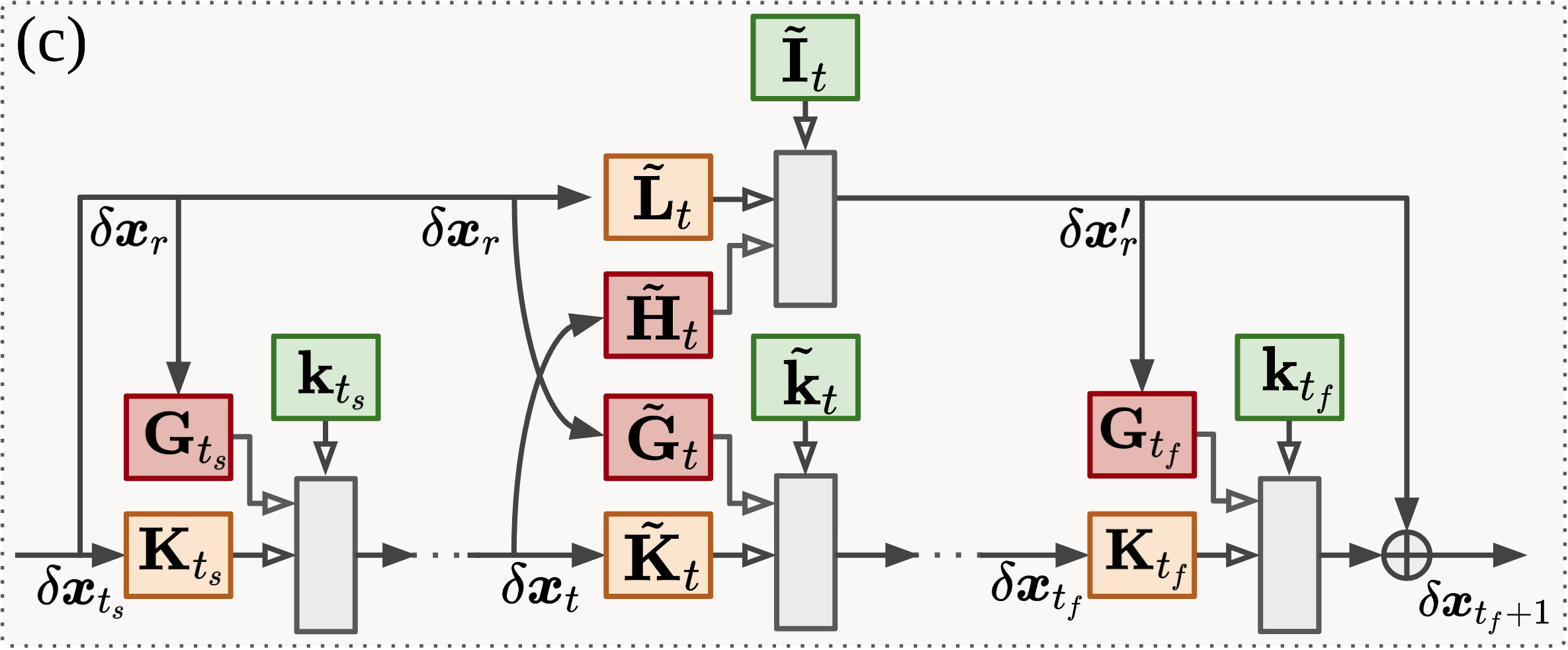
Figure 3: Terminology and weight update graph for (a) standard Back-propagation and (b)(c) GT-DDP optimizer with identity and arbitrary shortcut mapping.

3.2 Cooperative Trajectory Optimization with Non-identity Shortcut Mapping

In some cases, the dimension of feature map between tssubscript𝑡𝑠t_{s} and tfsubscript𝑡𝑓t_{f} may be mismatched; thus the residual path will contain a non-identity shortcut mapping [34]. For CNNs this is typically achieved by down-sampling 𝒙rsubscript𝒙𝑟{\bm{x}}_{r} with an 1×\times1 convolution. Hereafter we will denote this non-identity mapping as 𝒙r=ht(𝒙r,𝒗t)superscriptsubscript𝒙𝑟subscript𝑡subscript𝒙𝑟subscript𝒗𝑡{\bm{x}}_{r}^{\prime}=h_{t}({\bm{x}}_{r},{\bm{v}}_{t}), where 𝒗tsubscript𝒗𝑡{\bm{v}}_{t} is the vectorized weight. The new Bellman equation, consider for instance when we add the mapping to the middle of residual path, i.e. t(ts,tf)𝑡subscript𝑡𝑠subscript𝑡𝑓t\in(t_{s},t_{f}) in Eq. (17d), becomes

Vt(𝒙r,𝒙t)=min𝒖t,𝒗t(𝒖t)+(𝒗t)+Vt+1(ht(𝒙r,𝒗t),ft(𝒙t,𝒖t))Qt(𝒙r,𝒙t,𝒖t,𝒗t) .subscript𝑉𝑡subscript𝒙𝑟subscript𝒙𝑡subscriptsubscript𝒖𝑡subscript𝒗𝑡subscriptsubscript𝒖𝑡subscript𝒗𝑡subscript𝑉𝑡1subscript𝑡subscript𝒙𝑟subscript𝒗𝑡subscript𝑓𝑡subscript𝒙𝑡subscript𝒖𝑡absentsubscript𝑄𝑡subscript𝒙𝑟subscript𝒙𝑡subscript𝒖𝑡subscript𝒗𝑡 .\displaystyle V_{t}({\bm{x}}_{r},{\bm{x}}_{t})=\min_{{\bm{u}}_{t},{\bm{v}}_{t}}\underbrace{\ell({\bm{u}}_{t})+\ell({\bm{v}}_{t})+V_{t+1}(h_{t}({\bm{x}}_{r},{\bm{v}}_{t}),f_{t}({\bm{x}}_{t},{\bm{u}}_{t}))}_{\triangleq Q_{t}({\bm{x}}_{r},{\bm{x}}_{t},{\bm{u}}_{t},{\bm{v}}_{t})}{\text{ .}} (22)

Minimizing Qt(𝒙r,𝒙t,𝒖t,𝒗t)subscript𝑄𝑡subscript𝒙𝑟subscript𝒙𝑡subscript𝒖𝑡subscript𝒗𝑡Q_{t}({\bm{x}}_{r},{\bm{x}}_{t},{\bm{u}}_{t},{\bm{v}}_{t}) simultaneously wrt 𝒖tsubscript𝒖𝑡{\bm{u}}_{t} and 𝒗tsubscript𝒗𝑡{\bm{v}}_{t} resembles the formulation in a complete Cooperative Game (CG) [35]. In its common setup, two players observe the same state and decide their policies to maximize a cooperative payoff. The game is complete in that all information is known and shared in prior; thus can be leveraged to make better decisions. Application of DDP to solving CG has been studied previously in robotics for robust trajectory optimization [36].

Before solving Eq. (22), it will be useful to first revisit cases when each policy can be solved independently, i.e. when Qt(𝒙r,𝒙t,𝒖t,𝒗t)=Qt(𝒙t,𝒖t)+Qt(𝒙r,𝒗t)subscript𝑄𝑡subscript𝒙𝑟subscript𝒙𝑡subscript𝒖𝑡subscript𝒗𝑡subscript𝑄𝑡subscript𝒙𝑡subscript𝒖𝑡subscript𝑄𝑡subscript𝒙𝑟subscript𝒗𝑡Q_{t}({\bm{x}}_{r},{\bm{x}}_{t},{\bm{u}}_{t},{\bm{v}}_{t})=Q_{t}({\bm{x}}_{t},{\bm{u}}_{t})+Q_{t}({\bm{x}}_{r},{\bm{v}}_{t}). In this case, we know 𝐤t,𝐊tsubscript𝐤𝑡subscript𝐊𝑡{\mathbf{k}_{t}},{\mathbf{K}_{t}} is the solution to argmin𝒖tQt(𝒙t,𝒖t)subscriptargminsubscript𝒖𝑡subscript𝑄𝑡subscript𝒙𝑡subscript𝒖𝑡\operatorname*{arg\,min}_{{\bm{u}}_{t}}Q_{t}({\bm{x}}_{t},{\bm{u}}_{t}). Let us further denote 𝐈t+𝐋tδ𝒙r=argmin𝒗tQt(𝒙r,𝒗t)subscript𝐈𝑡subscript𝐋𝑡𝛿subscript𝒙𝑟subscriptargminsubscript𝒗𝑡subscript𝑄𝑡subscript𝒙𝑟subscript𝒗𝑡{\mathbf{I}_{t}}+{\mathbf{L}_{t}}{\delta{\bm{x}}}_{r}=\operatorname*{arg\,min}_{{\bm{v}}_{t}}Q_{t}({\bm{x}}_{r},{\bm{v}}_{t}), where 𝐈t(Q𝒗𝒗t)1Q𝒗tsubscript𝐈𝑡superscriptsubscriptsuperscript𝑄𝑡𝒗𝒗1subscriptsuperscript𝑄𝑡𝒗{\mathbf{I}_{t}}\triangleq-({Q^{t}_{{\bm{v}}{\bm{v}}}})^{-1}{Q^{t}_{{\bm{v}}}} and 𝐋t(Q𝒗𝒗t)1Q𝒗𝒙rtsubscript𝐋𝑡superscriptsubscriptsuperscript𝑄𝑡𝒗𝒗1subscriptsuperscript𝑄𝑡𝒗subscript𝒙𝑟{\mathbf{L}_{t}}\triangleq-({Q^{t}_{{\bm{v}}{\bm{v}}}})^{-1}{Q^{t}_{{\bm{v}}{\bm{x}}_{r}}}. Now, solving Eq. (22) by quadratically expanding Qt(𝒙r,𝒙t,𝒖t,𝒗t)subscript𝑄𝑡subscript𝒙𝑟subscript𝒙𝑡subscript𝒖𝑡subscript𝒗𝑡Q_{t}({\bm{x}}_{r},{\bm{x}}_{t},{\bm{u}}_{t},{\bm{v}}_{t}) wrt all variables will arrive at the following form333 We omit the superscript t𝑡t of Q𝒖𝒖1subscriptsuperscript𝑄1𝒖𝒖{Q^{-1}_{{\bm{u}}{\bm{u}}}},Q𝒗𝒗1subscriptsuperscript𝑄1𝒗𝒗{Q^{-1}_{{\bm{v}}{\bm{v}}}},Q~𝒖𝒖1subscriptsuperscript~𝑄1𝒖𝒖{\tilde{Q}^{-1}_{{\bm{u}}{\bm{u}}}},Q~𝒗𝒗1subscriptsuperscript~𝑄1𝒗𝒗{\tilde{Q}^{-1}_{{\bm{v}}{\bm{v}}}} sometimes for notational simplicity but stress that Q𝑄Q is always time (i.e. layer) dependent in this work. :

δ𝒖t(δ𝒙t,δ𝒙r)=𝛿superscriptsubscript𝒖𝑡𝛿subscript𝒙𝑡𝛿subscript𝒙𝑟absent\displaystyle{\delta{\bm{u}}}_{t}^{*}({\delta{\bm{x}}}_{t},{\delta{\bm{x}}}_{r})= 𝐤~t+𝐊~tδ𝒙t+𝐆~tδ𝒙rsubscript~𝐤𝑡subscript~𝐊𝑡𝛿subscript𝒙𝑡subscript~𝐆𝑡𝛿subscript𝒙𝑟\displaystyle{\color[rgb]{0,0.5,0}\definecolor[named]{pgfstrokecolor}{rgb}{0,0.5,0}{\tilde{\mathbf{k}}_{t}}}+{\color[rgb]{0.95,0.475,0}\definecolor[named]{pgfstrokecolor}{rgb}{0.95,0.475,0}{\tilde{\mathbf{K}}_{t}}}{\delta{\bm{x}}}_{t}+{\color[rgb]{0.8,0,0}\definecolor[named]{pgfstrokecolor}{rgb}{0.8,0,0}{\tilde{\mathbf{G}}_{t}}}{\delta{\bm{x}}}_{r} (23)
=\displaystyle= Q~𝒖𝒖1(Q𝒖t+Q𝒖𝒗t𝐈t+(Q𝒖𝒙tQ𝒖𝒗tQ𝒗𝒗1Q𝒗𝒙t)δ𝒙t+(Q𝒖𝒙rt+Q𝒖𝒗t𝐋t)δ𝒙r) ,subscriptsuperscript~𝑄1𝒖𝒖subscriptsuperscript𝑄𝑡𝒖subscriptsuperscript𝑄𝑡𝒖𝒗subscript𝐈𝑡subscriptsuperscript𝑄𝑡𝒖𝒙subscriptsuperscript𝑄𝑡𝒖𝒗subscriptsuperscript𝑄1𝒗𝒗subscriptsuperscript𝑄𝑡𝒗𝒙𝛿subscript𝒙𝑡subscriptsuperscript𝑄𝑡𝒖subscript𝒙𝑟subscriptsuperscript𝑄𝑡𝒖𝒗subscript𝐋𝑡𝛿subscript𝒙𝑟 ,\displaystyle-{\tilde{Q}^{-1}_{{\bm{u}}{\bm{u}}}}\Big{(}\text{\textul{${Q^{t}_{{\bm{u}}}}+{Q^{t}_{{\bm{u}}{\bm{v}}}}{\mathbf{I}_{t}}$}}+\text{\textul{$({Q^{t}_{{\bm{u}}{\bm{x}}}}-{Q^{t}_{{\bm{u}}{\bm{v}}}}{Q^{-1}_{{\bm{v}}{\bm{v}}}}{Q^{t}_{{\bm{v}}{\bm{x}}}})$}}{\delta{\bm{x}}}_{t}+\text{\textul{$({Q^{t}_{{\bm{u}}{\bm{x}}_{r}}}+{Q^{t}_{{\bm{u}}{\bm{v}}}}{\mathbf{L}_{t}})$}}{\delta{\bm{x}}}_{r}\Big{)}{\text{ ,}}
δ𝒗t(δ𝒙t,δ𝒙r)=𝛿superscriptsubscript𝒗𝑡𝛿subscript𝒙𝑡𝛿subscript𝒙𝑟absent\displaystyle{\delta{\bm{v}}}_{t}^{*}({\delta{\bm{x}}}_{t},{\delta{\bm{x}}}_{r})= 𝐈~t+𝐋~tδ𝒙r+𝐇~tδ𝒙tsubscript~𝐈𝑡subscript~𝐋𝑡𝛿subscript𝒙𝑟subscript~𝐇𝑡𝛿subscript𝒙𝑡\displaystyle{\color[rgb]{0,0.5,0}\definecolor[named]{pgfstrokecolor}{rgb}{0,0.5,0}{\tilde{\mathbf{I}}_{t}}}+{\color[rgb]{0.95,0.475,0}\definecolor[named]{pgfstrokecolor}{rgb}{0.95,0.475,0}{\tilde{\mathbf{L}}_{t}}}{\delta{\bm{x}}}_{r}+{\color[rgb]{0.8,0,0}\definecolor[named]{pgfstrokecolor}{rgb}{0.8,0,0}{\tilde{\mathbf{H}}_{t}}}{\delta{\bm{x}}}_{t} (24)
=\displaystyle= Q~𝒗𝒗1(Q𝒗t+Q𝒗𝒖t𝐤t+(Q𝒗𝒙rtQ𝒗𝒖tQ𝒖𝒖1Q𝒖𝒙rt)δ𝒙r+(Q𝒗𝒙t+Q𝒗𝒖t𝐊t)δ𝒙t),subscriptsuperscript~𝑄1𝒗𝒗subscriptsuperscript𝑄𝑡𝒗subscriptsuperscript𝑄𝑡𝒗𝒖subscript𝐤𝑡subscriptsuperscript𝑄𝑡𝒗subscript𝒙𝑟subscriptsuperscript𝑄𝑡𝒗𝒖subscriptsuperscript𝑄1𝒖𝒖subscriptsuperscript𝑄𝑡𝒖subscript𝒙𝑟𝛿subscript𝒙𝑟subscriptsuperscript𝑄𝑡𝒗𝒙subscriptsuperscript𝑄𝑡𝒗𝒖subscript𝐊𝑡𝛿subscript𝒙𝑡\displaystyle-{\tilde{Q}^{-1}_{{\bm{v}}{\bm{v}}}}\Big{(}\text{\textul{${Q^{t}_{{\bm{v}}}}+{Q^{t}_{{\bm{v}}{\bm{u}}}}{\mathbf{k}_{t}}$}}+\text{\textul{$({Q^{t}_{{\bm{v}}{\bm{x}}_{r}}}-{Q^{t}_{{\bm{v}}{\bm{u}}}}{Q^{-1}_{{\bm{u}}{\bm{u}}}}{Q^{t}_{{\bm{u}}{\bm{x}}_{r}}})$}}{\delta{\bm{x}}}_{r}+\text{\textul{$({Q^{t}_{{\bm{v}}{\bm{x}}}}+{Q^{t}_{{\bm{v}}{\bm{u}}}}{\mathbf{K}_{t}})$}}{\delta{\bm{x}}}_{t}\Big{)},

where Q~𝒖𝒖tQ𝒖𝒖tQ𝒖𝒗tQ𝒗𝒗1Q𝒗𝒖tsubscriptsuperscript~𝑄𝑡𝒖𝒖subscriptsuperscript𝑄𝑡𝒖𝒖subscriptsuperscript𝑄𝑡𝒖𝒗subscriptsuperscript𝑄1𝒗𝒗subscriptsuperscript𝑄𝑡𝒗𝒖{\tilde{Q}^{t}_{{\bm{u}}{\bm{u}}}}\triangleq{Q^{t}_{{\bm{u}}{\bm{u}}}}-{Q^{t}_{{\bm{u}}{\bm{v}}}}{Q^{-1}_{{\bm{v}}{\bm{v}}}}{Q^{t}_{{\bm{v}}{\bm{u}}}} and Q~𝒗𝒗tQ𝒗𝒗tQ𝒗𝒖tQ𝒖𝒖1Q𝒖𝒗tsubscriptsuperscript~𝑄𝑡𝒗𝒗subscriptsuperscript𝑄𝑡𝒗𝒗subscriptsuperscript𝑄𝑡𝒗𝒖subscriptsuperscript𝑄1𝒖𝒖subscriptsuperscript𝑄𝑡𝒖𝒗{\tilde{Q}^{t}_{{\bm{v}}{\bm{v}}}}\triangleq{Q^{t}_{{\bm{v}}{\bm{v}}}}-{Q^{t}_{{\bm{v}}{\bm{u}}}}{Q^{-1}_{{\bm{u}}{\bm{u}}}}{Q^{t}_{{\bm{u}}{\bm{v}}}} result from the block-matrices inversion with the Schur complement. The update rules provided in Eq. (23, 24) are much complex and do not admit forms of superposition as in Eq. (18). To make some intuitions, compare for instance the open gain 𝐤tQ𝒖𝒖1Q𝒖tsubscript𝐤𝑡subscriptsuperscript𝑄1𝒖𝒖subscriptsuperscript𝑄𝑡𝒖{\mathbf{k}_{t}}\triangleq-{Q^{-1}_{{\bm{u}}{\bm{u}}}}{Q^{t}_{{\bm{u}}}} with its cooperative variant 𝐤~tQ~𝒖𝒖1(Q𝒖t+Q𝒖𝒗t𝐈t)subscript~𝐤𝑡subscriptsuperscript~𝑄1𝒖𝒖subscriptsuperscript𝑄𝑡𝒖subscriptsuperscript𝑄𝑡𝒖𝒗subscript𝐈𝑡{\tilde{\mathbf{k}}_{t}}\triangleq-{\tilde{Q}^{-1}_{{\bm{u}}{\bm{u}}}}({Q^{t}_{{\bm{u}}}}+{Q^{t}_{{\bm{u}}{\bm{v}}}}{\mathbf{I}_{t}}). The latter adjusts the policy by knowing the companion’s update rule 𝐈tsubscript𝐈𝑡{\mathbf{I}_{t}}, and information between two players’ actions communicates through Q𝒖𝒗subscript𝑄𝒖𝒗{Q_{{\bm{u}}{\bm{v}}}} and Q𝒗𝒖subscript𝑄𝒗𝒖{Q_{{\bm{v}}{\bm{u}}}}. Similar interpretation can be drawn for the feedback gains 𝐊tsubscript𝐊𝑡{\mathbf{K}_{t}} and 𝐊~tsubscript~𝐊𝑡{\tilde{\mathbf{K}}_{t}}, as Q𝒗𝒖subscript𝑄𝒗𝒖{Q_{{\bm{v}}{\bm{u}}}} allows information to flow from Q𝒖𝒙subscript𝑄𝒖𝒙{Q_{{\bm{u}}{\bm{x}}}} through Q𝒗𝒙subscript𝑄𝒗𝒙{Q_{{\bm{v}}{\bm{x}}}}, and etc.

Fig. 3c illustrates how these feedback policies generate the weight update. 𝐤tsubscript𝐤𝑡{\mathbf{k}_{t}} and 𝐊tsubscript𝐊𝑡{\mathbf{K}_{t}} are applied in the same manner as in feedforward networks (c.f. Fig. 2). Layers parallel to the skip connection receive additional residual feedback from 𝐆tsubscript𝐆𝑡{\mathbf{G}_{t}}. At the decision stage when the non-identity shortcut mapping is involved, policies will be modified to their cooperative form, i.e. 𝐤~t,𝐊~t,𝐆~t,𝐈~t,𝐋~t,𝐇~tsubscript~𝐤𝑡subscript~𝐊𝑡subscript~𝐆𝑡subscript~𝐈𝑡subscript~𝐋𝑡subscript~𝐇𝑡{\tilde{\mathbf{k}}_{t}},{\tilde{\mathbf{K}}_{t}},{\tilde{\mathbf{G}}_{t}},{\tilde{\mathbf{I}}_{t}},{\tilde{\mathbf{L}}_{t}},{\tilde{\mathbf{H}}_{t}}. Notice that the residual policies 𝐆stsubscript𝐆𝑠𝑡\mathbf{G}_{s\leq t} and 𝐆s>tsubscript𝐆𝑠𝑡\mathbf{G}_{s>t} now take different state differential (δ𝒙r𝛿subscript𝒙𝑟\delta{\bm{x}}_{r} and δ𝒙r𝛿subscriptsuperscript𝒙𝑟\delta{\bm{x}}^{\prime}_{r} resp.). This implies the GT-DDP solution to residual networks is not unique, as placing ht(𝒙r,𝒗t)subscript𝑡subscript𝒙𝑟subscript𝒗𝑡h_{t}({\bm{x}}_{r},{\bm{v}}_{t}) at different location along the shortcut will result in different value of weight update. Despite seemly unintuitive, from the game theoretic perspective it implies one would prefer δ𝒙r𝛿subscriptsuperscript𝒙𝑟\delta{\bm{x}}^{\prime}_{r} to δ𝒙r𝛿subscript𝒙𝑟\delta{\bm{x}}_{r} whenever the former is available, since states closer to the decision stage reveal more information.

4 Game Theoretic DDP Neural Optimizer

Table 1: Relation between existing first (e.g. RMSprop) and
second-order (e.g. EKFAC) algorithms under GT-DDP framework444 direct-product\odot denotes element-wise multiplication. 𝒉𝒉{\bm{h}} is the pre-activation vector defined in Sec. 4.
    Q𝒖𝒖subscript𝑄𝒖𝒖{Q_{{\bm{u}}{\bm{u}}}},Q𝒗𝒗subscript𝑄𝒗𝒗{Q_{{\bm{v}}{\bm{v}}}} Q𝒖𝒗subscript𝑄𝒖𝒗{Q_{{\bm{u}}{\bm{v}}}},Q𝒗𝒖subscript𝑄𝒗𝒖{Q_{{\bm{v}}{\bm{u}}}} nonzero Q𝒖𝒙subscript𝑄𝒖𝒙{Q_{{\bm{u}}{\bm{x}}}},
    Q𝒗𝒙rsubscript𝑄𝒗subscript𝒙𝑟{Q_{{\bm{v}}{\bm{x}}_{r}}},Q𝒖𝒙rsubscript𝑄𝒖subscript𝒙𝑟{Q_{{\bm{u}}{\bm{x}}_{r}}}, Q𝒗𝒙subscript𝑄𝒗𝒙{Q_{{\bm{v}}{\bm{x}}}}
RMSprop    1ηdiag(J𝒖J𝒖+ϵ)1𝜂diagdirect-productsubscript𝐽𝒖subscript𝐽𝒖italic-ϵ\frac{1}{\eta}\operatorname{diag}({J}_{\bm{u}}\odot{J}_{\bm{u}}+\epsilon) 𝟎0\mathbf{0}
GT-DDP-RMSprop    1ηdiag(Q𝒖Q𝒖+ϵ)1𝜂diagdirect-productsubscript𝑄𝒖subscript𝑄𝒖italic-ϵ\frac{1}{\eta}\operatorname{diag}({Q}_{\bm{u}}\odot{Q}_{\bm{u}}+\epsilon) 𝟎0\mathbf{0}
EKFAC    𝔼[𝒙𝒙𝖳]𝔼[J𝒉J𝒉𝖳]tensor-product𝔼delimited-[]𝒙superscript𝒙𝖳𝔼delimited-[]subscript𝐽𝒉superscriptsubscript𝐽𝒉𝖳\mathbb{E}[{\bm{x}}{\bm{x}}^{\mathsf{T}}]\otimes\mathbb{E}[{J_{\bm{h}}}J_{\bm{h}}^{\mathsf{T}}] 𝟎0\mathbf{0}
GT-DDP-EKFAC    𝔼[𝒙𝒙𝖳]𝔼[V𝒉V𝒉𝖳]tensor-product𝔼delimited-[]𝒙superscript𝒙𝖳𝔼delimited-[]subscript𝑉𝒉superscriptsubscript𝑉𝒉𝖳\mathbb{E}[{\bm{x}}{\bm{x}}^{\mathsf{T}}]\otimes\mathbb{E}[{V_{\bm{h}}}V_{\bm{h}}^{\mathsf{T}}] Theorem 3

In this section we discuss efficient computation of the update rules proposed in the previous section to training residual networks. As the algorithm generalizes the DDP framework [1] to new architectures under game-theoretic perspective, we name it the Game Theoretic DDP neural optimizer (GT-DDP). Detailed derivation and proof in this section are left in the Appendix B.

4.1 Curvature Approximation

Computation of the GT-DDP solution involves extensive evaluation of the derivatives of Qtsubscript𝑄𝑡Q_{t} wrt different variables. Since ftsubscript𝑓𝑡f_{t} is highly over-parametrized in each network layer, second-order derivatives wrt the weight parameter, e.g. Q𝒖𝒖tsubscriptsuperscript𝑄𝑡𝒖𝒖{Q^{t}_{{\bm{u}}{\bm{u}}}} Q𝒗𝒗tsubscriptsuperscript𝑄𝑡𝒗𝒗{Q^{t}_{{\bm{v}}{\bm{v}}}}, are particularly expansive to compute, let alone their inversions. Thus, approximation must be made for these matrices.

Following the curvature interpretation in Sec 2.1, one can simply substitute these expansive Hessians with the ones considered in existing methods. For instance, replacing Q𝒖𝒖tsubscriptsuperscript𝑄𝑡𝒖𝒖{Q^{t}_{{\bm{u}}{\bm{u}}}} with an identity (or diagonal) matrix resembles the (adaptive) first-order update rule. Note that this first-order approximation implicitly implies both Q𝒖𝒗tsubscriptsuperscript𝑄𝑡𝒖𝒗{Q^{t}_{{\bm{u}}{\bm{v}}}} and Q𝒗𝒖tsubscriptsuperscript𝑄𝑡𝒗𝒖{Q^{t}_{{\bm{v}}{\bm{u}}}} to vanish, since by construction first-order methods omit the covariances among different weight coordinate.

As for second-order approximation, in this work we consider the popular Kronecker factorization used in EKFAC [31]. Let ftσ(𝑾t𝒙tf_{t}\equiv\sigma({\bm{W}}_{t}{\bm{x}}_{t}+𝒃t){\bm{b}}_{t}) be the generic dynamics where σ𝜎\sigma is the activation function, and denote 𝒉t𝑾t𝒙t+𝒃tsubscript𝒉𝑡subscript𝑾𝑡subscript𝒙𝑡subscript𝒃𝑡{\bm{h}}_{t}\equiv{\bm{W}}_{t}{\bm{x}}_{t}+{\bm{b}}_{t} as the pre-activation vector. EKFAC factorizes Q𝒖𝒖t𝔼[𝒙t𝒙t𝖳]𝔼[𝒈t𝒈t𝖳]superscriptsubscript𝑄𝒖𝒖𝑡tensor-product𝔼delimited-[]subscript𝒙𝑡superscriptsubscript𝒙𝑡𝖳𝔼delimited-[]subscript𝒈𝑡superscriptsubscript𝒈𝑡𝖳Q_{{\bm{u}}{\bm{u}}}^{t}\approx\mathbb{E}[{\bm{x}}_{t}{\bm{x}}_{t}^{\mathsf{T}}]\otimes\mathbb{E}[{\bm{g}}_{t}{\bm{g}}_{t}^{\mathsf{T}}], where tensor-product\otimes is the Kronecker operator and 𝒈t:=J𝒉tassignsubscript𝒈𝑡subscriptsuperscript𝐽𝑡𝒉{\bm{g}}_{t}:=J^{t}_{{\bm{h}}} is the first-order derivative of the per-stage objective wrt the pre-activation vector555 For GT-DDP-EKFAC, we have 𝒈t:=V𝒉tassignsubscript𝒈𝑡subscriptsuperscript𝑉𝑡𝒉{\bm{g}}_{t}:=V^{t}_{{\bm{h}}}. We left further introduction and derivation in Appendix B.1. . The expectation is taken wrt the batch sample. Factorizing GT-DDP with Kronecker operation requires one to derive the Kronecker representations for the cooperative matrices appeared in CG, which are given below.

Theorem 3 (Kronecker factorization in Cooperative Game).

Suppose Q𝐮𝐮subscript𝑄𝐮𝐮{Q_{{\bm{u}}{\bm{u}}}} and Q𝐯𝐯subscript𝑄𝐯𝐯{Q_{{\bm{v}}{\bm{v}}}} are factorized respectively by Q𝐮𝐮A𝐮𝐮B𝐮𝐮subscript𝑄𝐮𝐮tensor-productsubscript𝐴𝐮𝐮subscript𝐵𝐮𝐮Q_{{\bm{u}}{\bm{u}}}\approx{A_{{\bm{u}}{\bm{u}}}}\otimes{B_{{\bm{u}}{\bm{u}}}} and Q𝐯𝐯A𝐯𝐯B𝐯𝐯subscript𝑄𝐯𝐯tensor-productsubscript𝐴𝐯𝐯subscript𝐵𝐯𝐯Q_{{\bm{v}}{\bm{v}}}\approx{A_{{\bm{v}}{\bm{v}}}}\otimes{B_{{\bm{v}}{\bm{v}}}}, where

A𝒖𝒖𝔼[𝒙𝒖𝒙𝒖𝖳] ,B𝒖𝒖𝔼[𝒈𝒖𝒈𝒖𝖳] ,A𝒗𝒗𝔼[𝒙𝒗𝒙𝒗𝖳] ,B𝒗𝒗𝔼[𝒈𝒗𝒈𝒗𝖳]formulae-sequencesubscript𝐴𝒖𝒖𝔼delimited-[]subscript𝒙𝒖superscriptsubscript𝒙𝒖𝖳 ,formulae-sequencesubscript𝐵𝒖𝒖𝔼delimited-[]subscript𝒈𝒖superscriptsubscript𝒈𝒖𝖳 ,formulae-sequencesubscript𝐴𝒗𝒗𝔼delimited-[]subscript𝒙𝒗superscriptsubscript𝒙𝒗𝖳 ,subscript𝐵𝒗𝒗𝔼delimited-[]subscript𝒈𝒗superscriptsubscript𝒈𝒗𝖳\displaystyle{A_{{\bm{u}}{\bm{u}}}}\triangleq{\mathbb{E}[{\bm{x}}_{{\bm{u}}}{\bm{x}}_{{\bm{u}}}^{\mathsf{T}}]}{\text{ ,}}\quad{B_{{\bm{u}}{\bm{u}}}}\triangleq{\mathbb{E}[{\bm{g}}_{{\bm{u}}}{\bm{g}}_{{\bm{u}}}^{\mathsf{T}}]}{\text{ ,}}\quad{A_{{\bm{v}}{\bm{v}}}}\triangleq{\mathbb{E}[{\bm{x}}_{{\bm{v}}}{\bm{x}}_{{\bm{v}}}^{\mathsf{T}}]}{\text{ ,}}\quad{B_{{\bm{v}}{\bm{v}}}}\triangleq{\mathbb{E}[{\bm{g}}_{{\bm{v}}}{\bm{g}}_{{\bm{v}}}^{\mathsf{T}}]}

are the Kronecker block matrices for layers f(𝐱𝐮,𝐮)𝑓subscript𝐱𝐮𝐮f({\bm{x}}_{\bm{u}},{\bm{u}}) and h(𝐱𝐯,𝐯)subscript𝐱𝐯𝐯h({\bm{x}}_{\bm{v}},{\bm{v}}). Further, let A𝐮𝐯𝔼[𝐱𝐮𝐱𝐯𝖳]subscript𝐴𝐮𝐯𝔼delimited-[]subscript𝐱𝐮superscriptsubscript𝐱𝐯𝖳{A_{{\bm{u}}{\bm{v}}}}\triangleq{\mathbb{E}[{\bm{x}}_{{\bm{u}}}{\bm{x}}_{{\bm{v}}}^{\mathsf{T}}]} and B𝐮𝐯𝔼[𝐠𝐮𝐠𝐯𝖳]subscript𝐵𝐮𝐯𝔼delimited-[]subscript𝐠𝐮superscriptsubscript𝐠𝐯𝖳{B_{{\bm{u}}{\bm{v}}}}\triangleq{\mathbb{E}[{\bm{g}}_{{\bm{u}}}{\bm{g}}_{{\bm{v}}}^{\mathsf{T}}]}, then the unique Kronecker factorizations for the matrices in CG are given by

Q~𝒖𝒖1subscriptsuperscript~𝑄1𝒖𝒖\displaystyle{\tilde{Q}^{-1}_{{\bm{u}}{\bm{u}}}} A~𝒖𝒖1B~𝒖𝒖1=(A𝒖𝒖A𝒖𝒗A𝒗𝒗1A𝒖𝒗𝖳)1(B𝒖𝒖B𝒖𝒗B𝒗𝒗1B𝒖𝒗𝖳)1absenttensor-productsubscriptsuperscript~𝐴1𝒖𝒖subscriptsuperscript~𝐵1𝒖𝒖tensor-productsuperscriptsubscript𝐴𝒖𝒖subscript𝐴𝒖𝒗subscriptsuperscript𝐴1𝒗𝒗subscriptsuperscript𝐴𝖳𝒖𝒗1superscriptsubscript𝐵𝒖𝒖subscript𝐵𝒖𝒗subscriptsuperscript𝐵1𝒗𝒗subscriptsuperscript𝐵𝖳𝒖𝒗1\displaystyle\approx{\tilde{A}^{-1}_{{\bm{u}}{\bm{u}}}}\otimes{\tilde{B}^{-1}_{{\bm{u}}{\bm{u}}}}=({A_{{\bm{u}}{\bm{u}}}}-{A_{{\bm{u}}{\bm{v}}}}{A^{-1}_{{\bm{v}}{\bm{v}}}}{A^{\mathsf{T}}_{{\bm{u}}{\bm{v}}}})^{-1}\otimes({B_{{\bm{u}}{\bm{u}}}}-{B_{{\bm{u}}{\bm{v}}}}{B^{-1}_{{\bm{v}}{\bm{v}}}}{B^{\mathsf{T}}_{{\bm{u}}{\bm{v}}}})^{-1} (25)
Q~𝒗𝒗1subscriptsuperscript~𝑄1𝒗𝒗\displaystyle{\tilde{Q}^{-1}_{{\bm{v}}{\bm{v}}}} A~𝒗𝒗1B~𝒗𝒗1=(A𝒗𝒗A𝒖𝒗𝖳A𝒖𝒖1A𝒖𝒗)1(B𝒗𝒗B𝒖𝒗𝖳B𝒖𝒖1B𝒖𝒗)1 ,absenttensor-productsubscriptsuperscript~𝐴1𝒗𝒗subscriptsuperscript~𝐵1𝒗𝒗tensor-productsuperscriptsubscript𝐴𝒗𝒗subscriptsuperscript𝐴𝖳𝒖𝒗subscriptsuperscript𝐴1𝒖𝒖subscript𝐴𝒖𝒗1superscriptsubscript𝐵𝒗𝒗subscriptsuperscript𝐵𝖳𝒖𝒗subscriptsuperscript𝐵1𝒖𝒖subscript𝐵𝒖𝒗1 ,\displaystyle\approx{\tilde{A}^{-1}_{{\bm{v}}{\bm{v}}}}\otimes{\tilde{B}^{-1}_{{\bm{v}}{\bm{v}}}}=({A_{{\bm{v}}{\bm{v}}}}-{A^{\mathsf{T}}_{{\bm{u}}{\bm{v}}}}{A^{-1}_{{\bm{u}}{\bm{u}}}}{A_{{\bm{u}}{\bm{v}}}})^{-1}\otimes({B_{{\bm{v}}{\bm{v}}}}-{B^{\mathsf{T}}_{{\bm{u}}{\bm{v}}}}{B^{-1}_{{\bm{u}}{\bm{u}}}}{B_{{\bm{u}}{\bm{v}}}})^{-1}{\text{ ,}} (26)

and Q𝐮𝐯=Q𝐯𝐮𝖳A𝐮𝐯B𝐮𝐯subscript𝑄𝐮𝐯subscriptsuperscript𝑄𝖳𝐯𝐮tensor-productsubscript𝐴𝐮𝐯subscript𝐵𝐮𝐯{Q_{{\bm{u}}{\bm{v}}}}={Q^{\mathsf{T}}_{{\bm{v}}{\bm{u}}}}\approx-{A_{{\bm{u}}{\bm{v}}}}\otimes{B_{{\bm{u}}{\bm{v}}}}. The CG update, take 𝐤~tsubscript~𝐤𝑡{\tilde{\mathbf{k}}_{t}} for example, can be computed by

𝐤~t=vec(B~𝒖𝒖1(Q𝒖+B𝒖𝒗B𝒗𝒗1Q𝒗A𝒗𝒗𝖳A𝒖𝒗𝖳)A~𝒖𝒖𝖳) .subscript~𝐤𝑡vecsubscriptsuperscript~𝐵1𝒖𝒖subscript𝑄𝒖subscript𝐵𝒖𝒗subscriptsuperscript𝐵1𝒗𝒗subscript𝑄𝒗subscriptsuperscript𝐴𝖳𝒗𝒗subscriptsuperscript𝐴𝖳𝒖𝒗subscriptsuperscript~𝐴𝖳𝒖𝒖 .\displaystyle{\tilde{\mathbf{k}}_{t}}=-\mathrm{vec}({\tilde{B}^{-1}_{{\bm{u}}{\bm{u}}}}({Q_{{\bm{u}}}}+{B_{{\bm{u}}{\bm{v}}}}{B^{-1}_{{\bm{v}}{\bm{v}}}}{Q_{{\bm{v}}}}{A^{-{\mathsf{T}}}_{{\bm{v}}{\bm{v}}}}{A^{\mathsf{T}}_{{\bm{u}}{\bm{v}}}}){\tilde{A}^{-{\mathsf{T}}}_{{\bm{u}}{\bm{u}}}}){\text{ .}} (27)

Hereafter we will refer these approximations respectively to GT-DDP-RMSprop, GT-DDP-EKFAC, and etc. The algorithmic relation between existing methods and their DDP integration is summarized in Table 1, with the theoretical connection given by the following proposition.

Proposition 4.

The update rules derived from stage-wise minimization of the Bellman equation degenerate to the method it uses to approximate the weight Hessian, i.e. Q𝐮𝐮subscript𝑄𝐮𝐮{Q_{{\bm{u}}{\bm{u}}}} Q𝐯𝐯subscript𝑄𝐯𝐯{Q_{{\bm{v}}{\bm{v}}}}, when the Bellman objective Qtsubscript𝑄𝑡Q_{t} at all stages satisfies (i) all mixed partial derivatives between parameter and activation, e.g. Q𝐮𝐱subscript𝑄𝐮𝐱{Q_{{\bm{u}}{\bm{x}}}},Q𝐮𝐱rsubscript𝑄𝐮subscript𝐱𝑟{Q_{{\bm{u}}{\bm{x}}_{r}}}, vanish, and (ii) parameters between distinct layers are uncorrelated.

Note that Proposition 4 extends Proposition 1 to arbitrary architectures beyond feedforward and residual networks, so long as its layer-wise Bellman objective is properly defined.

4.2 Practical Implementation

Refer to caption
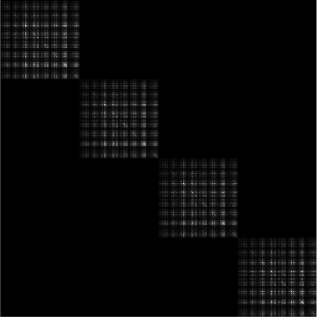
Figure 4: Example of V𝒙𝒙tsubscriptsuperscript𝑉𝑡superscript𝒙superscript𝒙V^{t}_{{\bm{x}}^{\prime}{\bm{x}}^{\prime}} for batch size B=4𝐵4B=4 in DIGITS dataset. Higher (whiter) values concentrate along the diagonal blocks V𝒙(i)𝒙(i)tsubscriptsuperscript𝑉𝑡superscript𝒙𝑖superscript𝒙𝑖V^{t}_{{\bm{x}}^{(i)}{\bm{x}}^{(i)}}

Block-diagonal Value Hessian: Extending the Bellman optimization framework to accept mini-batch samples {𝒙0(i)}i=0Bsuperscriptsubscriptsuperscriptsubscript𝒙0𝑖𝑖0𝐵\{{\bm{x}}_{0}^{(i)}\}_{i=0}^{B} has been made in previous work [1] by augmenting the state space to 𝒙t=[,𝒙t(i),]𝖳superscriptsubscript𝒙𝑡superscriptsuperscriptsubscript𝒙𝑡𝑖𝖳{\bm{x}}_{t}^{\prime}=[\cdots,{\bm{x}}_{t}^{(i)},\cdots]^{\mathsf{T}}. However, such a formulation can cause memory explosion when 𝒙tsubscript𝒙𝑡{\bm{x}}_{t} is lifted to 3D feature map in convolutional layers, let alone the augmented value function considered in GT-DDP (cf Eq. (17)). In this work, we propose to approximate the batch-augmented value Hessian V𝒙𝒙tsubscriptsuperscript𝑉𝑡superscript𝒙superscript𝒙V^{t}_{{\bm{x}}^{\prime}{\bm{x}}^{\prime}} as block-diagonal. The approximation is made from an empirical observation (see Fig. 4) that V𝒙𝒙tsubscriptsuperscript𝑉𝑡superscript𝒙superscript𝒙V^{t}_{{\bm{x}}^{\prime}{\bm{x}}^{\prime}} contains only nontrivial values along the diagonal blocks, even when networks contain Batch Normalization (BN) layers. This suggests one can reduce the memory consumption by approximating the batch-augmented value Hessian as block-diagonal and only carry batch matrices, {V𝒙(i)𝒙(i)t}i=0Bsuperscriptsubscriptsubscriptsuperscript𝑉𝑡superscript𝒙𝑖superscript𝒙𝑖𝑖0𝐵\{V^{t}_{{\bm{x}}^{(i)}{\bm{x}}^{(i)}}\}_{i=0}^{B}, along the backward computation.

Gauss-Newton (GN) Approximation at the Terminal Hessian: Next,
we impose Gauss-Newton approximation to the Hessian at the prediction
layer. Surprisingly, this will lead to a nontrivial factorization in the Bellman optimization framework. For dynamics represented by feedforward networks, we have the following proposition.

Proposition 5 (Outer-product factorization in DDP).

Consider the following form of OCP:

min𝒖¯[ϕ(𝒙T)+t=0T1t(𝒖t)]s.t. 𝒙t+1=ft(𝒙t,𝒖t) .subscript¯𝒖italic-ϕsubscript𝒙𝑇superscriptsubscript𝑡0𝑇1subscript𝑡subscript𝒖𝑡s.t. subscript𝒙𝑡1subscript𝑓𝑡subscript𝒙𝑡subscript𝒖𝑡 .\min_{{\bar{{\bm{u}}}}}\left[\phi({\bm{x}}_{T})+\sum_{t=0}^{T-1}\ell_{t}({\bm{u}}_{t})\right]\quad\text{s.t. }{\bm{x}}_{t+1}=f_{t}({\bm{x}}_{t},{\bm{u}}_{t}){\text{ .}} (28)

If the Hessian of the terminal loss can be expressed by an outer product of vectors, i.e. 2ϕ(𝐱T)𝐳𝐱T𝐳𝐱Tsuperscript2italic-ϕsubscript𝐱𝑇tensor-productsuperscriptsubscript𝐳𝐱𝑇superscriptsubscript𝐳𝐱𝑇\nabla^{2}\phi({\bm{x}}_{T})\approx{\bm{z}}_{\bm{x}}^{T}\otimes{\bm{z}}_{\bm{x}}^{T} for some vector 𝐳𝐱Tsuperscriptsubscript𝐳𝐱𝑇{\bm{z}}_{\bm{x}}^{T} (e.g. 𝐳𝐱T=ϕsuperscriptsubscript𝐳𝐱𝑇italic-ϕ{\bm{z}}_{\bm{x}}^{T}=\nabla\phi for GN approximation), then we have the factorization:

t ,Q𝒖𝒙t=𝒒𝒖t𝒒𝒙t ,Q𝒙𝒙t=𝒒𝒙t𝒒𝒙t ,V𝒙𝒙t=𝒛𝒙t𝒛𝒙t ,formulae-sequencefor-all𝑡 ,subscriptsuperscript𝑄𝑡𝒖𝒙tensor-productsuperscriptsubscript𝒒𝒖𝑡superscriptsubscript𝒒𝒙𝑡 ,formulae-sequencesubscriptsuperscript𝑄𝑡𝒙𝒙tensor-productsuperscriptsubscript𝒒𝒙𝑡superscriptsubscript𝒒𝒙𝑡 ,superscriptsubscript𝑉𝒙𝒙𝑡tensor-productsuperscriptsubscript𝒛𝒙𝑡superscriptsubscript𝒛𝒙𝑡 ,\begin{split}\forall t{\text{ ,}}\quad{Q^{t}_{{\bm{u}}{\bm{x}}}}={\bm{q}}_{\bm{u}}^{t}\otimes{\bm{q}}_{\bm{x}}^{t}{\text{ ,}}\quad{Q^{t}_{{\bm{x}}{\bm{x}}}}={\bm{q}}_{\bm{x}}^{t}\otimes{\bm{q}}_{\bm{x}}^{t}{\text{ ,}}\quad V_{{\bm{x}}{\bm{x}}}^{t}={\bm{z}}_{\bm{x}}^{t}\otimes{\bm{z}}_{\bm{x}}^{t}{\text{ ,}}\quad\end{split} (29)

where 𝐪𝐮tsuperscriptsubscript𝐪𝐮𝑡{\bm{q}}_{\bm{u}}^{t}, 𝐪𝐱tsuperscriptsubscript𝐪𝐱𝑡{\bm{q}}_{\bm{x}}^{t}, and 𝐳𝐱tsuperscriptsubscript𝐳𝐱𝑡{\bm{z}}_{\bm{x}}^{t} are outer-product vectors which can be computed backward:

𝒒𝒖t=f𝒖t𝖳𝒛𝒙t+1 ,𝒒𝒙t=f𝒙t𝖳𝒛𝒙t+1 ,𝒛𝒙t=1+𝐪𝐮t 𝖳(Q𝐮𝐮t)1𝐪𝐮t  𝒒𝒙t .formulae-sequencesuperscriptsubscript𝒒𝒖𝑡superscriptsubscriptsuperscript𝑓𝑡𝒖𝖳superscriptsubscript𝒛𝒙𝑡1 ,formulae-sequencesuperscriptsubscript𝒒𝒙𝑡superscriptsubscriptsuperscript𝑓𝑡𝒙𝖳superscriptsubscript𝒛𝒙𝑡1 ,superscriptsubscript𝒛𝒙𝑡1+𝐪𝐮t 𝖳(Q𝐮𝐮t)1𝐪𝐮t  superscriptsubscript𝒒𝒙𝑡 .\displaystyle{\bm{q}}_{\bm{u}}^{t}={{{f}^{t}_{{\bm{u}}}}^{\mathsf{T}}}{\bm{z}}_{\bm{x}}^{t+1}{\text{ ,}}\quad{\bm{q}}_{\bm{x}}^{t}={{{f}^{t}_{{\bm{x}}}}^{\mathsf{T}}}{\bm{z}}_{\bm{x}}^{t+1}{\text{ ,}}\quad{\bm{z}}_{\bm{x}}^{t}=\mathchoice{{\hbox{$\displaystyle\sqrt{1+{\bm{q}}_{\bm{u}}^{t\text{ }{\mathsf{T}}}{({Q^{t}_{{\bm{u}}{\bm{u}}})}^{-1}}{\bm{q}}_{\bm{u}}^{t}\,}$}\lower 0.4pt\hbox{\vrule height=10.35999pt,depth=-8.28802pt}}}{{\hbox{$\textstyle\sqrt{1+{\bm{q}}_{\bm{u}}^{t\text{ }{\mathsf{T}}}{({Q^{t}_{{\bm{u}}{\bm{u}}})}^{-1}}{\bm{q}}_{\bm{u}}^{t}\,}$}\lower 0.4pt\hbox{\vrule height=10.35999pt,depth=-8.28802pt}}}{{\hbox{$\scriptstyle\sqrt{1+{\bm{q}}_{\bm{u}}^{t\text{ }{\mathsf{T}}}{({Q^{t}_{{\bm{u}}{\bm{u}}})}^{-1}}{\bm{q}}_{\bm{u}}^{t}\,}$}\lower 0.4pt\hbox{\vrule height=7.30237pt,depth=-5.84192pt}}}{{\hbox{$\scriptscriptstyle\sqrt{1+{\bm{q}}_{\bm{u}}^{t\text{ }{\mathsf{T}}}{({Q^{t}_{{\bm{u}}{\bm{u}}})}^{-1}}{\bm{q}}_{\bm{u}}^{t}\,}$}\lower 0.4pt\hbox{\vrule height=5.9357pt,depth=-4.74858pt}}}\text{ }{\bm{q}}_{\bm{x}}^{t}{\text{ .}} (30)

In other words, the outer-product factorization at the final stage can be backward propagated to all proceeding layers. Thus, state-dependent second-order matrices can be represented as outer products of vectors. We note that the low-rank structure at the prediction layer has been observed when classification loss (e.g. cross-entropy) is used [37, 38]. Prop. 5 can be extended to residual networks:

Proposition 6 (Outer-product factorization in GT-DDP).

The residual value Hessians considered in Eq. (19), when the same outer-product factorization is imposed at the terminal stage, take the form

V𝒙𝒙rt=𝒛𝒙t𝒛𝒙rt  and  V𝒙r𝒙rt=𝒛𝒙rt𝒛𝒙rt ,  where 𝒛𝒙rt=1+𝐪𝐮t 𝖳(Q𝐮𝐮t)1𝐪𝐮t  𝒛𝒙rt+1subscriptsuperscript𝑉𝑡𝒙subscript𝒙𝑟tensor-productsuperscriptsubscript𝒛𝒙𝑡superscriptsubscript𝒛subscript𝒙𝑟𝑡  and  subscriptsuperscript𝑉𝑡subscript𝒙𝑟subscript𝒙𝑟tensor-productsuperscriptsubscript𝒛subscript𝒙𝑟𝑡superscriptsubscript𝒛subscript𝒙𝑟𝑡 ,  where superscriptsubscript𝒛subscript𝒙𝑟𝑡1+𝐪𝐮t 𝖳(Q𝐮𝐮t)1𝐪𝐮t  superscriptsubscript𝒛subscript𝒙𝑟𝑡1\begin{split}V^{t}_{{\bm{x}}{{\bm{x}}_{r}}}={\bm{z}}_{\bm{x}}^{t}\otimes{\bm{z}}_{{\bm{x}}_{r}}^{t}\text{ }\text{ and }\text{ }V^{t}_{{{\bm{x}}_{r}}{{\bm{x}}_{r}}}={\bm{z}}_{{\bm{x}}_{r}}^{t}\otimes{\bm{z}}_{{\bm{x}}_{r}}^{t}{\text{ ,}}\text{ }\text{ where }{\bm{z}}_{{\bm{x}}_{r}}^{t}=\mathchoice{{\hbox{$\displaystyle\sqrt{1+{\bm{q}}_{\bm{u}}^{t\text{ }{\mathsf{T}}}{({Q^{t}_{{\bm{u}}{\bm{u}}})}^{-1}}{\bm{q}}_{\bm{u}}^{t}\,}$}\lower 0.4pt\hbox{\vrule height=10.35999pt,depth=-8.28802pt}}}{{\hbox{$\textstyle\sqrt{1+{\bm{q}}_{\bm{u}}^{t\text{ }{\mathsf{T}}}{({Q^{t}_{{\bm{u}}{\bm{u}}})}^{-1}}{\bm{q}}_{\bm{u}}^{t}\,}$}\lower 0.4pt\hbox{\vrule height=10.35999pt,depth=-8.28802pt}}}{{\hbox{$\scriptstyle\sqrt{1+{\bm{q}}_{\bm{u}}^{t\text{ }{\mathsf{T}}}{({Q^{t}_{{\bm{u}}{\bm{u}}})}^{-1}}{\bm{q}}_{\bm{u}}^{t}\,}$}\lower 0.4pt\hbox{\vrule height=7.30237pt,depth=-5.84192pt}}}{{\hbox{$\scriptscriptstyle\sqrt{1+{\bm{q}}_{\bm{u}}^{t\text{ }{\mathsf{T}}}{({Q^{t}_{{\bm{u}}{\bm{u}}})}^{-1}}{\bm{q}}_{\bm{u}}^{t}\,}$}\lower 0.4pt\hbox{\vrule height=5.9357pt,depth=-4.74858pt}}}\text{ }{\bm{z}}_{{\bm{x}}_{r}}^{t+1}\end{split} (31)

and (𝐪𝐮t,𝐪𝐱t,𝐳𝐱t)superscriptsubscript𝐪𝐮𝑡superscriptsubscript𝐪𝐱𝑡superscriptsubscript𝐳𝐱𝑡({\bm{q}}_{\bm{u}}^{t},{\bm{q}}_{\bm{x}}^{t},{\bm{z}}_{\bm{x}}^{t}) are given by Eq. (30). When the non-identity shortcut mapping, i.e. ht(𝐱r,𝐯t)subscript𝑡subscript𝐱𝑟subscript𝐯𝑡h_{t}({\bm{x}}_{r},{\bm{v}}_{t}) in Eq. (22), is presented, the cooperative forms of 𝐳𝐱tsuperscriptsubscript𝐳𝐱𝑡{\bm{z}}_{\bm{x}}^{t} and 𝐳𝐱rtsuperscriptsubscript𝐳subscript𝐱𝑟𝑡{\bm{z}}_{{\bm{x}}_{r}}^{t}, denoted 𝐳~𝐱tsuperscriptsubscript~𝐳𝐱𝑡\tilde{{\bm{z}}}_{\bm{x}}^{t} and 𝐳~𝐱rtsuperscriptsubscript~𝐳subscript𝐱𝑟𝑡\tilde{{\bm{z}}}_{{\bm{x}}_{r}}^{t}, are given by

𝒛~𝒙t=1+𝐪𝐮t 𝖳Q𝐮𝐮1𝐪𝐮t+𝐪𝐯t 𝖳Q𝐯𝐯1𝐪𝐯t  𝒒𝒙t ,𝒛~𝒙rt=1+𝐪𝐮t 𝖳Q𝐮𝐮1𝐪𝐮t+𝐪𝐯t 𝖳Q𝐯𝐯1𝐪𝐯t  𝒒𝒙rt,formulae-sequencesuperscriptsubscript~𝒛𝒙𝑡1+𝐪𝐮t 𝖳Q𝐮𝐮1𝐪𝐮t+𝐪𝐯t 𝖳Q𝐯𝐯1𝐪𝐯t  superscriptsubscript𝒒𝒙𝑡 ,superscriptsubscript~𝒛subscript𝒙𝑟𝑡1+𝐪𝐮t 𝖳Q𝐮𝐮1𝐪𝐮t+𝐪𝐯t 𝖳Q𝐯𝐯1𝐪𝐯t  superscriptsubscript𝒒subscript𝒙𝑟𝑡\begin{split}\tilde{{\bm{z}}}_{\bm{x}}^{t}=\mathchoice{{\hbox{$\displaystyle\sqrt{1+{\bm{q}}_{\bm{u}}^{t\text{ }{\mathsf{T}}}{Q^{-1}_{{\bm{u}}{\bm{u}}}}{\bm{q}}_{\bm{u}}^{t}+{\bm{q}}_{\bm{v}}^{t\text{ }{\mathsf{T}}}{Q^{-1}_{{\bm{v}}{\bm{v}}}}{\bm{q}}_{\bm{v}}^{t}\,}$}\lower 0.4pt\hbox{\vrule height=8.63776pt,depth=-6.91023pt}}}{{\hbox{$\textstyle\sqrt{1+{\bm{q}}_{\bm{u}}^{t\text{ }{\mathsf{T}}}{Q^{-1}_{{\bm{u}}{\bm{u}}}}{\bm{q}}_{\bm{u}}^{t}+{\bm{q}}_{\bm{v}}^{t\text{ }{\mathsf{T}}}{Q^{-1}_{{\bm{v}}{\bm{v}}}}{\bm{q}}_{\bm{v}}^{t}\,}$}\lower 0.4pt\hbox{\vrule height=8.63776pt,depth=-6.91023pt}}}{{\hbox{$\scriptstyle\sqrt{1+{\bm{q}}_{\bm{u}}^{t\text{ }{\mathsf{T}}}{Q^{-1}_{{\bm{u}}{\bm{u}}}}{\bm{q}}_{\bm{u}}^{t}+{\bm{q}}_{\bm{v}}^{t\text{ }{\mathsf{T}}}{Q^{-1}_{{\bm{v}}{\bm{v}}}}{\bm{q}}_{\bm{v}}^{t}\,}$}\lower 0.4pt\hbox{\vrule height=6.0722pt,depth=-4.85779pt}}}{{\hbox{$\scriptscriptstyle\sqrt{1+{\bm{q}}_{\bm{u}}^{t\text{ }{\mathsf{T}}}{Q^{-1}_{{\bm{u}}{\bm{u}}}}{\bm{q}}_{\bm{u}}^{t}+{\bm{q}}_{\bm{v}}^{t\text{ }{\mathsf{T}}}{Q^{-1}_{{\bm{v}}{\bm{v}}}}{\bm{q}}_{\bm{v}}^{t}\,}$}\lower 0.4pt\hbox{\vrule height=4.70554pt,depth=-3.76445pt}}}\text{ }{\bm{q}}_{\bm{x}}^{t}{\text{ ,}}\quad\tilde{{\bm{z}}}_{{\bm{x}}_{r}}^{t}=\mathchoice{{\hbox{$\displaystyle\sqrt{1+{\bm{q}}_{\bm{u}}^{t\text{ }{\mathsf{T}}}{Q^{-1}_{{\bm{u}}{\bm{u}}}}{\bm{q}}_{\bm{u}}^{t}+{\bm{q}}_{\bm{v}}^{t\text{ }{\mathsf{T}}}{Q^{-1}_{{\bm{v}}{\bm{v}}}}{\bm{q}}_{\bm{v}}^{t}\,}$}\lower 0.4pt\hbox{\vrule height=8.63776pt,depth=-6.91023pt}}}{{\hbox{$\textstyle\sqrt{1+{\bm{q}}_{\bm{u}}^{t\text{ }{\mathsf{T}}}{Q^{-1}_{{\bm{u}}{\bm{u}}}}{\bm{q}}_{\bm{u}}^{t}+{\bm{q}}_{\bm{v}}^{t\text{ }{\mathsf{T}}}{Q^{-1}_{{\bm{v}}{\bm{v}}}}{\bm{q}}_{\bm{v}}^{t}\,}$}\lower 0.4pt\hbox{\vrule height=8.63776pt,depth=-6.91023pt}}}{{\hbox{$\scriptstyle\sqrt{1+{\bm{q}}_{\bm{u}}^{t\text{ }{\mathsf{T}}}{Q^{-1}_{{\bm{u}}{\bm{u}}}}{\bm{q}}_{\bm{u}}^{t}+{\bm{q}}_{\bm{v}}^{t\text{ }{\mathsf{T}}}{Q^{-1}_{{\bm{v}}{\bm{v}}}}{\bm{q}}_{\bm{v}}^{t}\,}$}\lower 0.4pt\hbox{\vrule height=6.0722pt,depth=-4.85779pt}}}{{\hbox{$\scriptscriptstyle\sqrt{1+{\bm{q}}_{\bm{u}}^{t\text{ }{\mathsf{T}}}{Q^{-1}_{{\bm{u}}{\bm{u}}}}{\bm{q}}_{\bm{u}}^{t}+{\bm{q}}_{\bm{v}}^{t\text{ }{\mathsf{T}}}{Q^{-1}_{{\bm{v}}{\bm{v}}}}{\bm{q}}_{\bm{v}}^{t}\,}$}\lower 0.4pt\hbox{\vrule height=4.70554pt,depth=-3.76445pt}}}\text{ }{\bm{q}}_{{\bm{x}}_{r}}^{t},\end{split} (32)

where 𝐪𝐱rt=h𝐱rt 𝖳𝐳𝐱rt+1superscriptsubscript𝐪subscript𝐱𝑟𝑡superscriptsubscriptsubscript𝐱𝑟𝑡 𝖳superscriptsubscript𝐳subscript𝐱𝑟𝑡1{\bm{q}}_{{\bm{x}}_{r}}^{t}=h_{{{\bm{x}}_{r}}}^{t\text{ }{\mathsf{T}}}{\bm{z}}_{{\bm{x}}_{r}}^{t+1}, and 𝐪𝐯t=h𝐯t 𝖳𝐳𝐱rt+1superscriptsubscript𝐪𝐯𝑡superscriptsubscript𝐯𝑡 𝖳superscriptsubscript𝐳subscript𝐱𝑟𝑡1{\bm{q}}_{\bm{v}}^{t}=h_{{\bm{v}}}^{t\text{ }{\mathsf{T}}}{\bm{z}}_{{\bm{x}}_{r}}^{t+1}.

The outer-product factorization, together with the block-diagonal approximation, reduces the computational dependency by dropping the memory by 2/3232/3 and the runtime by 1/5151/5 compared with previous work [1], as shown in Fig. 1. As such, we adopt both approximation in all experiments.

Jacobian of Layers Dynamics: Finally, computing the derivatives of the Bellman objective involve evaluating the Jacobian associated with each layer, e.g. Q𝒙t=f𝒙t𝖳V𝒙t+1subscriptsuperscript𝑄𝑡𝒙superscriptsubscriptsuperscript𝑓𝑡𝒙𝖳subscriptsuperscript𝑉𝑡1𝒙Q^{t}_{{\bm{x}}}={f^{t}_{{\bm{x}}}}^{\mathsf{T}}V^{t+1}_{{\bm{x}}} and Q𝒖t=f𝒖t𝖳V𝒙t+1subscriptsuperscript𝑄𝑡𝒖superscriptsubscriptsuperscript𝑓𝑡𝒖𝖳subscriptsuperscript𝑉𝑡1𝒙Q^{t}_{{\bm{u}}}={f^{t}_{{\bm{u}}}}^{\mathsf{T}}V^{t+1}_{{\bm{x}}}. These computations can be done efficiently for both fully-connected (FC) and convolution (Conv) layers:

f𝒙t𝖳V𝒙t+1={𝑾t𝖳V𝒉tωt𝖳 ^ V𝒉t ,f𝒙t𝖳V𝒙t+1={𝒙tV𝒉t𝒙t ^ V𝒉t ,where f𝒙t=σt(𝒉t) ,𝒉t{𝑾t𝒙t+𝒃tωt𝒙tformulae-sequencesuperscriptsubscriptsuperscript𝑓𝑡𝒙𝖳subscriptsuperscript𝑉𝑡1𝒙casessuperscriptsubscript𝑾𝑡𝖳subscriptsuperscript𝑉𝑡𝒉superscriptsubscript𝜔𝑡𝖳 ^ subscriptsuperscript𝑉𝑡𝒉 ,formulae-sequencesuperscriptsubscriptsuperscript𝑓𝑡𝒙𝖳subscriptsuperscript𝑉𝑡1𝒙casestensor-productsubscript𝒙𝑡subscriptsuperscript𝑉𝑡𝒉subscript𝒙𝑡 ^ subscriptsuperscript𝑉𝑡𝒉 ,formulae-sequencewhere subscriptsuperscript𝑓𝑡𝒙subscript𝜎𝑡subscript𝒉𝑡 ,subscript𝒉𝑡casessubscript𝑾𝑡subscript𝒙𝑡subscript𝒃𝑡subscript𝜔𝑡subscript𝒙𝑡\displaystyle{f^{t}_{{\bm{x}}}}^{\mathsf{T}}V^{t+1}_{{\bm{x}}}=\Big{\{}\begin{array}[]{l}{{\bm{W}}_{t}^{\mathsf{T}}V^{t}_{{\bm{h}}}}\\ {\omega_{t}^{\mathsf{T}}{\text{ }\hat{*}\text{ }}V^{t}_{{\bm{h}}}}\end{array}{\text{ ,}}\quad{f^{t}_{{\bm{x}}}}^{\mathsf{T}}V^{t+1}_{{\bm{x}}}=\Big{\{}\begin{array}[]{l}{{\bm{x}}_{t}\otimes V^{t}_{{\bm{h}}}}\\ {{\bm{x}}_{t}{\text{ }\hat{*}\text{ }}V^{t}_{{\bm{h}}}}\end{array}{\text{ ,}}\quad\text{where }f^{t}_{{\bm{x}}}=\sigma_{t}({\bm{h}}_{t}){\text{ ,}}\quad{\bm{h}}_{t}\triangleq\Big{\{}\begin{array}[]{l}{{\bm{W}}_{t}{\bm{x}}_{t}+{\bm{b}}_{t}}\\ {\omega_{t}*{\bm{x}}_{t}}\end{array}

respectively denote the pre-activation of FC and Conv layers. * and  ^  ^ {\text{ }\hat{*}\text{ }} denote the convolution and deconvolution (transposed convolution) operator [39, 40].

5 Evaluation on Classification Data Set

Table 2: Performance comparison on train loss and validation accuracy (over 666 random seeds).
(+) and (-) respectively denote improvement and degradation over non-GT-DDP baselines.
Data Set   SGD RMSProp Adam EKFAC
GT-DDP
-SGD
GT-DDP
-RMSProp
GT-DDP
-Adam
GT-DDP
-EKFAC
Training DIGITS   0.00530.00530.0053 0.02470.02470.0247 0.01820.01820.0182 0.05140.05140.0514 0.0050 (+) 0.01240.01240.0124 (+) 0.00810.00810.0081 (+) 0.05140.05140.0514 (+)
MNIST   0.02500.02500.0250 0.02840.02840.0284 0.03300.03300.0330 0.02900.02900.0290 0.0240 (+) 0.02820.02820.0282 (+) 0.03120.03120.0312 (+) 0.02910.02910.0291 (-)
SVHN   0.27550.27550.2755 0.26700.26700.2670 0.25440.2544{0.2544} 0.20490.2049{0.2049} 0.26920.2692{0.2692} (+) 0.26370.26370.2637 (+) 0.25170.2517{0.2517} (+) 0.2047 (+)
CIFAR-10   0.02960.02960.0296 0.01070.01070.0107 0.01270.01270.0127 0.09220.09220.0922 0.02840.0284{0.0284} (+) 0.0069 (+) 0.00960.00960.0096 (+) 0.09070.09070.0907 (+)
CIFAR-100   0.00750.00750.0075 0.00580.00580.0058 0.00550.00550.0055 0.01200.01200.0120 0.00750.0075{0.0075} (-) 0.00580.0058{0.0058} (+) 0.0054 (+) 0.01250.01250.0125 (-)
Validation (%) DIGITS   96.0996.0996.09 95.6195.6195.61 95.8195.8195.81 95.3195.3195.31 96.10 (+) 95.9295.9295.92 (+) 95.8495.8495.84 (+) 95.5595.5595.55 (+)
MNIST   98.5998.5998.59 98.5298.5298.52 98.5198.5198.51 98.5698.5698.56 98.62 (+) 98.5398.5398.53 (+) 98.5198.5198.51 (+) 98.5698.5698.56 (-)
SVHN   88.5888.5888.58 88.9688.9688.96 89.2089.20{89.20} 88.7588.7588.75 89.9089.90{89.90} (+) 89.0289.0289.02 (+) 89.22 (+) 89.9189.9189.91 (+)
CIFAR-10   74.6974.69{74.69} 70.8870.8870.88 72.5172.5172.51 74.3374.3374.33 74.69 (+) 70.9770.9770.97 (+) 72.6872.6872.68 (+) 74.1874.1874.18 (-)
CIFAR-100   71.7871.7871.78 71.6571.6571.65 71.9671.9671.96 71.9571.9571.95 72.0672.06{72.06} (+) 71.9171.9171.91 (+) 72.1972.1972.19 (+) 72.24 (+)
Refer to caption
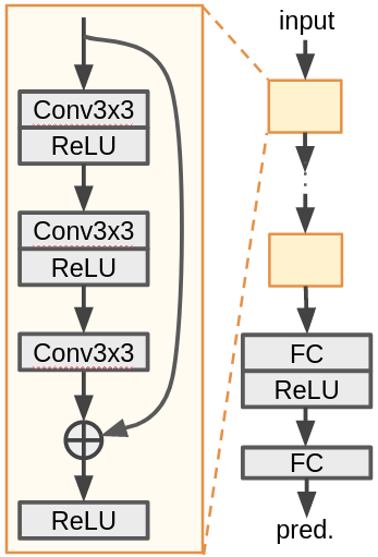
Figure 5: Architecture and residual block in Sec. 5.

In this section we verify the performance of our GT-DDP optimizer and discuss the benefit of having layer-wise feedback policies during weight update. Detail experiment setup and additional results are provided in the Appendix C.

We validate the performance of GT-DDP on digits recognition and image classification data set. The networks consist of 111-444 residual blocks followed by fully-connected (FC) layers (see Fig. 5), except that we use ResNet18 [21] for the CIFAR-100 dataset. Each block contains a skip connection between 333 convolution modules, possibly with a non-identity shortcut mapping if needed. Following the discussion in the previous section, we select our baselines as SGD, RMSprop [41], Adam [42], and EKFAC [31], as they cover most widely-used curvature approximation in training deep nets, including (adaptive) diagonal matrices and second-order Kronecker factorization.

Table 2 summarizes our main results. In each experiment we keep the shared hyper-parameters (e.g. learning rate and weight decay) between baselines and their GT-DDP variants the same, so that the performance difference only comes from GT-DDP framework. On all data set, GT-DDP achieves better or comparable results on both training and accuracy. Notably, when comparing original methods with their GT-DDP integrated variants, the latter improve training convergence on almost all dataset. Empirically, it also leads to better generalization.

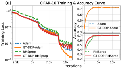
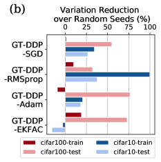
Since the feedback updates are typically order of magnitude smaller than the open gain due to the sparse Hessian of standard classification loss (i.e. cross-entropy), GT-DDP follows similar training trend with the baseline it used to approximate the parameter curvature (see Fig. 6a). Nevertheless, these additional updates have a non-trivial effect on not only improving the convergence but robustifying the training. As shown in Fig. 6b, GT-DDP reduces the variation of the performance difference over random seeds subjected to same hyper-parameters666 Additional experiments across different hyper-parameters are provided in the Appendix C.. In fact, the Bellman framework has been shown numerically stable than direct optimization such as Newton method [43], since it takes into account the temporal, i.e. layer-wise, structure inherit in Eq. (1). As the concern for reproducibility arises [44], GT-DDP provides a principled way to improve the robustness and consistency during training. We highlight this perspective as the benefit gained from architecture-aware optimization.

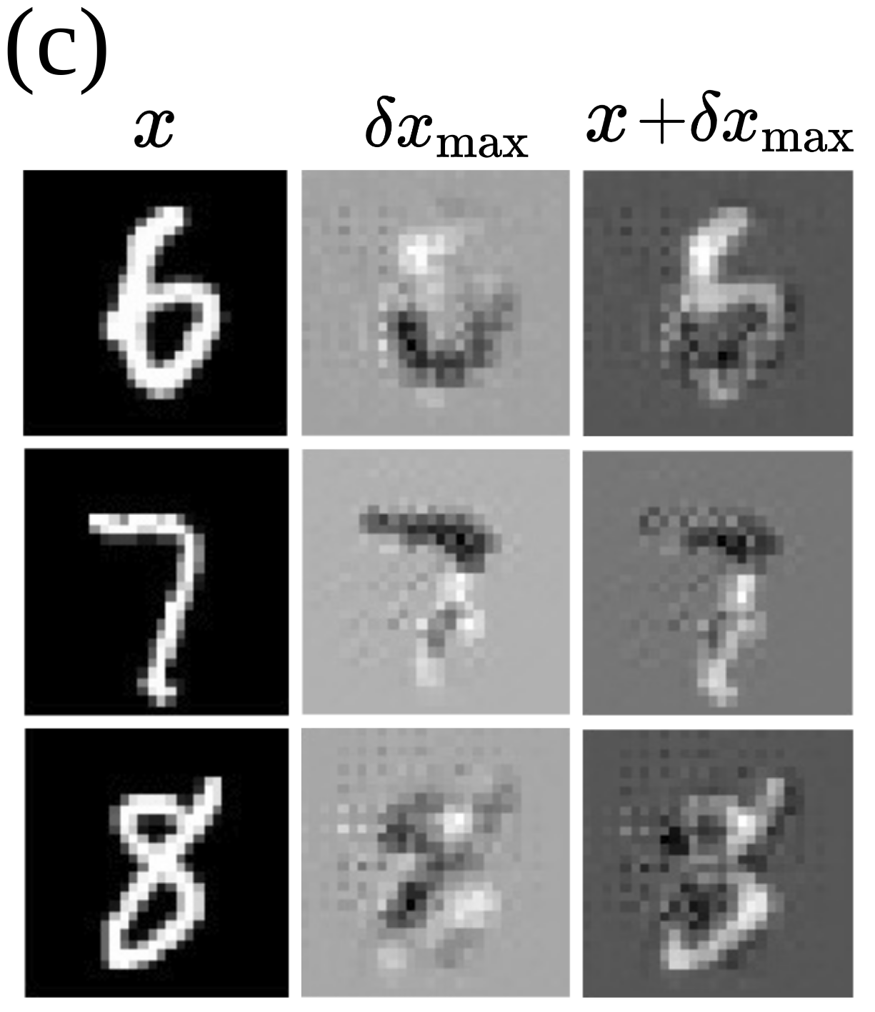
To understand the effect of feedback policies more perceptually, we conduct eigen-decomposition on the feedback matrices of convolution layers and project the leading eigenvectors back to image space, using techniques proposed in [45]. These feature maps, denoted δxmax𝛿subscript𝑥\delta x_{\max} in Fig. 6c, correspond to the dominating differential image that GT-DDP policies shall respond with during weight update. Fig. 6c demonstrates that the feedback policies indeed capture non-trivial visual feature related to the pixel-wise difference between spatially similar classes, e.g. (8,3)83(8,3) or (7,1)71(7,1). We note that these differential maps differ from adversarial perturbation [46] as the former directly link the parameter update to the change in activation; thus being more interpretable.
Refer to caption
(a)
Refer to caption
(b)
Refer to caption
(c)
Figure 6: (a) Training performance on CIFAR-10 for Adam, RMSprop and their GT-DDP variants. (b) Variation reduction over 333-666 random seeds on CIFAR-10 and CIFAR-100. We report the value (VARGT-DDP-BaselineVARBaseline)/VARBaselinesubscriptVARGT-DDP-BaselinesubscriptVARBaselinesubscriptVARBaseline(\mathrm{VAR}_{\text{GT-DDP-Baseline}}-\mathrm{VAR}_{\text{Baseline}})/\mathrm{VAR}_{\text{Baseline}}. (c) Visualization of the feedback policies on MNIST.

6 Discussion on Game-Theoretic Second-order Optimizer
Refer to caption
(a)
Refer to caption
(b)
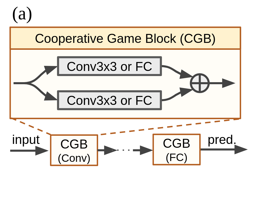
Figure 7: (a) Illustration of the cooperative-game module. (b) Training and testing performance on MNIST using the architecture in 7a. GT-EKFAC denotes integration of EKFAC with Corollary 7.

Theorem 3 may be of independent interest for developing game-theoretic second-order optimizer, as Eq.(25,26) provide efficient second-order approximation to the cooperative Hessian regardless of the presence of Bellman framework. To better show its effectiveness, let us consider the modules in Fig. 7a that resemble the cooperative game, i.e. two (p)layers take the same input and affect each payoff through output addition. Such an architecture has also appeared in recent work of progressive training [47]. Interestingly, for this particular structure, we have the following corollary to Thm. 3:

Corollary 7.

Let Q𝐮𝐮A𝐮𝐮B𝐮𝐮=𝐔Σ𝐮𝐮𝐔𝖳subscript𝑄𝐮𝐮tensor-productsubscript𝐴𝐮𝐮subscript𝐵𝐮𝐮𝐔subscriptΣ𝐮𝐮superscript𝐔𝖳Q_{{\bm{u}}{\bm{u}}}\approx{A_{{\bm{u}}{\bm{u}}}}\otimes{B_{{\bm{u}}{\bm{u}}}}={\bm{U}}\Sigma_{{\bm{u}}{\bm{u}}}{\bm{U}}^{\mathsf{T}} be the eigen-decomposition of the Kronecker factorization, where Σ𝐮𝐮=diag(λ𝐮𝐮)+γ𝐈subscriptΣ𝐮𝐮diagsubscript𝜆𝐮𝐮𝛾𝐈\Sigma_{{\bm{u}}{\bm{u}}}=\operatorname{diag}(\lambda_{{\bm{u}}{\bm{u}}})+\gamma{\bm{I}} and γ>0𝛾0\gamma>0 is the Tikhonov damping. Consider the architecture in Fig. 7a, its cooperative matrix corresponds to rescaling in the eigenspace of Q𝐮𝐮subscript𝑄𝐮𝐮{Q_{{\bm{u}}{\bm{u}}}}, i.e.

Q~𝒖𝒖=𝑼Σ~𝒖𝒖𝑼𝖳 ,Σ~𝒖𝒖=diag(λ~𝒖𝒖)+γ𝑰 ,and λ~𝒖𝒖i=γγ+λ𝒖𝒖iλ𝒖𝒖i .formulae-sequencesubscript~𝑄𝒖𝒖𝑼subscript~Σ𝒖𝒖superscript𝑼𝖳 ,formulae-sequencesubscript~Σ𝒖𝒖diagsubscript~𝜆𝒖𝒖𝛾𝑰 ,and superscriptsubscript~𝜆𝒖𝒖𝑖𝛾𝛾superscriptsubscript𝜆𝒖𝒖𝑖superscriptsubscript𝜆𝒖𝒖𝑖 .\displaystyle{\tilde{Q}_{{\bm{u}}{\bm{u}}}}={\bm{U}}\tilde{\Sigma}_{{\bm{u}}{\bm{u}}}{\bm{U}}^{\mathsf{T}}{\text{ ,}}\quad\tilde{\Sigma}_{{\bm{u}}{\bm{u}}}=\operatorname{diag}(\tilde{\lambda}_{{\bm{u}}{\bm{u}}})+\gamma{\bm{I}}{\text{ ,}}\quad\text{and }\quad\tilde{\lambda}_{{\bm{u}}{\bm{u}}}^{i}=\frac{\gamma}{\gamma+{\lambda}_{{\bm{u}}{\bm{u}}}^{i}}{\lambda}_{{\bm{u}}{\bm{u}}}^{i}{\text{ .}} (33)

Notice that γγ+λ𝒖𝒖i1𝛾𝛾superscriptsubscript𝜆𝒖𝒖𝑖1\frac{\gamma}{\gamma+{\lambda}_{{\bm{u}}{\bm{u}}}^{i}}\leq 1 for positive eigenvalues; thus the inverse Hessian Q~𝒖𝒖1subscriptsuperscript~𝑄1𝒖𝒖{\tilde{Q}^{-1}_{{\bm{u}}{\bm{u}}}} shall take a larger step in eigenspace compared with Q𝒖𝒖1subscriptsuperscript𝑄1𝒖𝒖{Q^{-1}_{{\bm{u}}{\bm{u}}}}. As shown in Fig 7b, integrating this game theoretic perspective with existing second-order methods, denoted GT-EKFAC, leads to better convergence. Having additional layer-wise policies from the GT-DDP framework further improves the performance.

7 Conclusion

In this work, we present the Game-Theoretic Differential Dynamic Programming (GT-DDP) optimizer as a new class of second-order algorithm. Theoretically, we strengthen the optimal control connection proposed in previous work by showing training residual networks can be linked to trajectory optimization in a cooperative game. Algorithmically, we propose several effective approximation which scales GT-DDP to training modern architectures and suggest how existing methods can be extended to accept such a game-theoretic perspective. We validate GT-DDP on several image classification dataset, showing improvement on both convergence and robustness.

Acknowledgments

The authors would like to thank Chen-Hsuan Lin, Yunpeng Pan, and Yen-Cheng Liu for many helpful discussions on the paper. The work is supported under Amazon AWS Machine Learning Research Award (MLRA).

References

  • Liu et al. [2020] Guan-Horng Liu, Tianrong Chen, and Evangelos A Theodorou. Differential dynamic programming neural optimizer. arXiv preprint arXiv:2002.08809, 2020.
  • Lu et al. [2017] Yiping Lu, Aoxiao Zhong, Quanzheng Li, and Bin Dong. Beyond finite layer neural networks: Bridging deep architectures and numerical differential equations. arXiv preprint arXiv:1710.10121, 2017.
  • Schoenholz et al. [2016] Samuel S Schoenholz, Justin Gilmer, Surya Ganguli, and Jascha Sohl-Dickstein. Deep information propagation. arXiv preprint arXiv:1611.01232, 2016.
  • Shwartz-Ziv and Tishby [2017] Ravid Shwartz-Ziv and Naftali Tishby. Opening the black box of deep neural networks via information. arXiv preprint arXiv:1703.00810, 2017.
  • Greydanus et al. [2019] Samuel Greydanus, Misko Dzamba, and Jason Yosinski. Hamiltonian neural networks. In Advances in Neural Information Processing Systems, pages 15353–15363, 2019.
  • Zhong et al. [2019] Yaofeng Desmond Zhong, Biswadip Dey, and Amit Chakraborty. Symplectic ode-net: Learning hamiltonian dynamics with control. arXiv preprint arXiv:1909.12077, 2019.
  • Weinan [2017] E Weinan. A proposal on machine learning via dynamical systems. Communications in Mathematics and Statistics, 5(1):1–11, 2017.
  • Lu et al. [2020] Yiping Lu, Chao Ma, Yulong Lu, Jianfeng Lu, and Lexing Ying. A mean-field analysis of deep resnet and beyond: Towards provable optimization via overparameterization from depth. arXiv preprint arXiv:2003.05508, 2020.
  • Sun et al. [2018] Qi Sun, Yunzhe Tao, and Qiang Du. Stochastic training of residual networks: a differential equation viewpoint. arXiv preprint arXiv:1812.00174, 2018.
  • Chang et al. [2018] Bo Chang, Lili Meng, Eldad Haber, Lars Ruthotto, David Begert, and Elliot Holtham. Reversible architectures for arbitrarily deep residual neural networks. In Thirty-Second AAAI Conference on Artificial Intelligence, 2018.
  • Haber and Ruthotto [2017] Eldad Haber and Lars Ruthotto. Stable architectures for deep neural networks. Inverse Problems, 34(1):014004, 2017.
  • Chen et al. [2018] Tian Qi Chen, Yulia Rubanova, Jesse Bettencourt, and David K Duvenaud. Neural ordinary differential equations. In Advances in Neural Information Processing Systems, pages 6572–6583, 2018.
  • Liu et al. [2019] Xuanqing Liu, Tesi Xiao, Si Si, Qin Cao, Sanjiv Kumar, and Cho-Jui Hsieh. Neural sde: Stabilizing neural ode networks with stochastic noise. arXiv preprint arXiv:1906.02355, 2019.
  • Tassa et al. [2012] Yuval Tassa, Tom Erez, and Emanuel Todorov. Synthesis and stabilization of complex behaviors through online trajectory optimization. In 2012 IEEE/RSJ International Conference on Intelligent Robots and Systems, pages 4906–4913. IEEE, 2012.
  • Weinan et al. [2018] E Weinan, Jiequn Han, and Qianxiao Li. A mean-field optimal control formulation of deep learning. arXiv preprint arXiv:1807.01083, 2018.
  • Liu and Theodorou [2019] Guan-Horng Liu and Evangelos A Theodorou. Deep learning theory review: An optimal control and dynamical systems perspective. arXiv preprint arXiv:1908.10920, 2019.
  • Li and Hao [2018] Qianxiao Li and Shuji Hao. An optimal control approach to deep learning and applications to discrete-weight neural networks. arXiv preprint arXiv:1803.01299, 2018.
  • Li et al. [2017] Qianxiao Li, Cheng Tai, and Weinan E. Stochastic modified equations and adaptive stochastic gradient algorithms. In Proceedings of the 34th International Conference on Machine Learning-Volume 70, pages 2101–2110. JMLR. org, 2017.
  • Zhang et al. [2019] Dinghuai Zhang, Tianyuan Zhang, Yiping Lu, Zhanxing Zhu, and Bin Dong. You only propagate once: Accelerating adversarial training via maximal principle. arXiv preprint arXiv:1905.00877, 2019.
  • Gunther et al. [2020] Stefanie Gunther, Lars Ruthotto, Jacob B Schroder, Eric C Cyr, and Nicolas R Gauger. Layer-parallel training of deep residual neural networks. SIAM Journal on Mathematics of Data Science, 2(1):1–23, 2020.
  • He et al. [2016a] Kaiming He, Xiangyu Zhang, Shaoqing Ren, and Jian Sun. Deep residual learning for image recognition. In Proceedings of the IEEE conference on computer vision and pattern recognition, pages 770–778, 2016a.
  • Goodfellow et al. [2014a] Ian Goodfellow, Jean Pouget-Abadie, Mehdi Mirza, Bing Xu, David Warde-Farley, Sherjil Ozair, Aaron Courville, and Yoshua Bengio. Generative adversarial nets. In Advances in neural information processing systems, pages 2672–2680, 2014a.
  • Kodali et al. [2017] Naveen Kodali, Jacob Abernethy, James Hays, and Zsolt Kira. On convergence and stability of gans. arXiv preprint arXiv:1705.07215, 2017.
  • Mescheder et al. [2017] Lars Mescheder, Sebastian Nowozin, and Andreas Geiger. The numerics of gans. In Advances in Neural Information Processing Systems, pages 1825–1835, 2017.
  • Balduzzi et al. [2018] David Balduzzi, Sebastien Racaniere, James Martens, Jakob Foerster, Karl Tuyls, and Thore Graepel. The mechanics of n-player differentiable games. arXiv preprint arXiv:1802.05642, 2018.
  • Balduzzi [2016] David Balduzzi. Grammars for games: a gradient-based, game-theoretic framework for optimization in deep learning. Frontiers in Robotics and AI, 2:39, 2016.
  • Ghorbani and Zou [2020] Amirata Ghorbani and James Zou. Neuron shapley: Discovering the responsible neurons. arXiv preprint arXiv:2002.09815, 2020.
  • Stier et al. [2018] Julian Stier, Gabriele Gianini, Michael Granitzer, and Konstantin Ziegler. Analysing neural network topologies: a game theoretic approach. Procedia Computer Science, 126:234–243, 2018.
  • Martens and Grosse [2015] James Martens and Roger Grosse. Optimizing neural networks with kronecker-factored approximate curvature. In International conference on machine learning, pages 2408–2417, 2015.
  • Grosse and Martens [2016] Roger Grosse and James Martens. A kronecker-factored approximate fisher matrix for convolution layers. In International Conference on Machine Learning, pages 573–582, 2016.
  • George et al. [2018] Thomas George, César Laurent, Xavier Bouthillier, Nicolas Ballas, and Pascal Vincent. Fast approximate natural gradient descent in a kronecker factored eigenbasis. In Advances in Neural Information Processing Systems, pages 9550–9560, 2018.
  • Bellman [1954] Richard Bellman. The theory of dynamic programming. Technical report, Rand corp santa monica ca, 1954.
  • Fan and Theodorou [2016] David D Fan and Evangelos A Theodorou. Differential dynamic programming for time-delayed systems. In 2016 IEEE 55th Conference on Decision and Control (CDC), pages 573–579. IEEE, 2016.
  • He et al. [2016b] Kaiming He, Xiangyu Zhang, Shaoqing Ren, and Jian Sun. Identity mappings in deep residual networks. In European conference on computer vision, pages 630–645. Springer, 2016b.
  • Yeung and Petrosjan [2006] David WK Yeung and Leon A Petrosjan. Cooperative stochastic differential games. Springer Science & Business Media, 2006.
  • Pan et al. [2015] Yunpeng Pan, Evangelos Theodorou, and Kaivalya Bakshi. Robust trajectory optimization: A cooperative stochastic game theoretic approach. In Robotics: Science and Systems, 2015.
  • Nar et al. [2019] Kamil Nar, Orhan Ocal, S Shankar Sastry, and Kannan Ramchandran. Cross-entropy loss and low-rank features have responsibility for adversarial examples. arXiv preprint arXiv:1901.08360, 2019.
  • Lezama et al. [2018] José Lezama, Qiang Qiu, Pablo Musé, and Guillermo Sapiro. Ole: Orthogonal low-rank embedding-a plug and play geometric loss for deep learning. In Proceedings of the IEEE Conference on Computer Vision and Pattern Recognition, pages 8109–8118, 2018.
  • Dumoulin and Visin [2016] Vincent Dumoulin and Francesco Visin. A guide to convolution arithmetic for deep learning. arXiv preprint arXiv:1603.07285, 2016.
  • Zeiler et al. [2010] Matthew D Zeiler, Dilip Krishnan, Graham W Taylor, and Rob Fergus. Deconvolutional networks. In 2010 IEEE Computer Society Conference on computer vision and pattern recognition, pages 2528–2535. IEEE, 2010.
  • Hinton et al. [2012] Geoffrey Hinton, Nitish Srivastava, and Kevin Swersky. Neural networks for machine learning lecture 6a overview of mini-batch gradient descent. 2012.
  • Kingma and Ba [2014] Diederik P Kingma and Jimmy Ba. Adam: A method for stochastic optimization. arXiv preprint arXiv:1412.6980, 2014.
  • Liao and Shoemaker [1992] Li-zhi Liao and Christine A Shoemaker. Advantages of differential dynamic programming over newton’s method for discrete-time optimal control problems. Technical report, Cornell University, 1992.
  • Henderson et al. [2018] Peter Henderson, Riashat Islam, Philip Bachman, Joelle Pineau, Doina Precup, and David Meger. Deep reinforcement learning that matters. In Thirty-Second AAAI Conference on Artificial Intelligence, 2018.
  • Zeiler and Fergus [2014] Matthew D Zeiler and Rob Fergus. Visualizing and understanding convolutional networks. In European conference on computer vision, pages 818–833. Springer, 2014.
  • Goodfellow et al. [2014b] Ian J Goodfellow, Jonathon Shlens, and Christian Szegedy. Explaining and harnessing adversarial examples. arXiv preprint arXiv:1412.6572, 2014b.
  • Wu et al. [2019] Lemeng Wu, Dilin Wang, and Qiang Liu. Splitting steepest descent for growing neural architectures. In Advances in Neural Information Processing Systems, pages 10655–10665, 2019.
  • Stein [2003] Gunter Stein. Respect the unstable. IEEE Control systems magazine, 23(4):12–25, 2003.
  • Todorov and Li [2005] Emanuel Todorov and Weiwei Li. A generalized iterative lqg method for locally-optimal feedback control of constrained nonlinear stochastic systems. In Proceedings of the 2005, American Control Conference, 2005., pages 300–306. IEEE, 2005.
  • Paszke et al. [2017] Adam Paszke, Sam Gross, Soumith Chintala, Gregory Chanan, Edward Yang, Zachary DeVito, Zeming Lin, Alban Desmaison, Luca Antiga, and Adam Lerer. Automatic differentiation in pytorch. 2017.

Supplementary Material

Appendix A Derivation of Optimal Control Representation for Residual networks

A.1 Derivation in Section 3.1

First, recall the Bellman objective in feedforward networks, Qt(𝒙t,𝒖t)t(𝒖t)+Vt+1(ft(𝒙t,𝒖t))subscript𝑄𝑡subscript𝒙𝑡subscript𝒖𝑡subscript𝑡subscript𝒖𝑡subscript𝑉𝑡1subscript𝑓𝑡subscript𝒙𝑡subscript𝒖𝑡Q_{t}({\bm{x}}_{t},{\bm{u}}_{t})\triangleq\ell_{t}({\bm{u}}_{t})+V_{t+1}(f_{t}({\bm{x}}_{t},{\bm{u}}_{t})). Following standard chain rule, the second-order expansion of Qtsubscript𝑄𝑡Q_{t} in Eq. (13) takes the form

δQt=12[𝟏δ𝒙tδ𝒖t]𝖳[𝟎Q𝒙t𝖳Q𝒖t𝖳Q𝒙tQ𝒙𝒙tQ𝒙𝒖tQ𝒖tQ𝒖𝒙tQ𝒖𝒖t][𝟏δ𝒙tδ𝒖t]Q𝒙t  =Q𝒖t  =Q𝒖𝒖t=Q𝒖𝒙t=Q𝒙𝒙t=f𝒙t𝖳V𝒙t+1f𝒖t𝖳V𝒙t+1+𝒖tf𝒖t𝖳V𝒙𝒙t+1f𝒖t+V𝒙t+1f𝒖𝒖t+𝒖𝒖tf𝒖t𝖳V𝒙𝒙t+1f𝒙t+V𝒙t+1f𝒖𝒙tf𝒙t𝖳V𝒙𝒙t+1f𝒙t+V𝒙t+1f𝒙𝒙t ,𝛿subscript𝑄𝑡12superscriptdelimited-[]1𝛿subscript𝒙𝑡𝛿subscript𝒖𝑡𝖳delimited-[]0superscriptsubscriptsuperscript𝑄𝑡𝒙𝖳superscriptsubscriptsuperscript𝑄𝑡𝒖𝖳subscriptsuperscript𝑄𝑡𝒙subscriptsuperscript𝑄𝑡𝒙𝒙subscriptsuperscript𝑄𝑡𝒙𝒖subscriptsuperscript𝑄𝑡𝒖subscriptsuperscript𝑄𝑡𝒖𝒙subscriptsuperscript𝑄𝑡𝒖𝒖delimited-[]1𝛿subscript𝒙𝑡𝛿subscript𝒖𝑡subscriptsuperscript𝑄𝑡𝒙  absentsubscriptsuperscript𝑄𝑡𝒖  absentsubscriptsuperscript𝑄𝑡𝒖𝒖absentsubscriptsuperscript𝑄𝑡𝒖𝒙absentsubscriptsuperscript𝑄𝑡𝒙𝒙absentsuperscriptsubscriptsuperscript𝑓𝑡𝒙𝖳subscriptsuperscript𝑉𝑡1𝒙superscriptsubscriptsuperscript𝑓𝑡𝒖𝖳subscriptsuperscript𝑉𝑡1𝒙subscriptsuperscript𝑡𝒖superscriptsubscriptsuperscript𝑓𝑡𝒖𝖳subscriptsuperscript𝑉𝑡1𝒙𝒙subscriptsuperscript𝑓𝑡𝒖subscriptsuperscript𝑉𝑡1𝒙subscriptsuperscript𝑓𝑡𝒖𝒖subscriptsuperscript𝑡𝒖𝒖superscriptsubscriptsuperscript𝑓𝑡𝒖𝖳subscriptsuperscript𝑉𝑡1𝒙𝒙subscriptsuperscript𝑓𝑡𝒙subscriptsuperscript𝑉𝑡1𝒙subscriptsuperscript𝑓𝑡𝒖𝒙superscriptsubscriptsuperscript𝑓𝑡𝒙𝖳subscriptsuperscript𝑉𝑡1𝒙𝒙subscriptsuperscript𝑓𝑡𝒙subscriptsuperscript𝑉𝑡1𝒙subscriptsuperscript𝑓𝑡𝒙𝒙 ,\displaystyle\delta Q_{t}=\frac{1}{2}\left[\begin{array}[]{c}\mathbf{1}\\ {\delta{\bm{x}}_{t}}\\ {\delta{\bm{u}}_{t}}\end{array}\right]^{{\mathsf{T}}}\left[\begin{array}[]{ccc}\mathbf{0}&{{Q^{t}_{{\bm{x}}}}^{{\mathsf{T}}}}&{{Q^{t}_{{\bm{u}}}}^{{\mathsf{T}}}}\\ {{Q^{t}_{{\bm{x}}}}}&{{Q^{t}_{{\bm{x}}{\bm{x}}}}}&{{Q^{t}_{{\bm{x}}{\bm{u}}}}}\\ {{Q^{t}_{{\bm{u}}}}}&{{Q^{t}_{{\bm{u}}{\bm{x}}}}}&{{Q^{t}_{{\bm{u}}{\bm{u}}}}}\end{array}\right]\left[\begin{array}[]{c}\mathbf{1}\\ {\delta{\bm{x}}_{t}}\\ {\delta{\bm{u}}_{t}}\end{array}\right]\text{, }\begin{array}[]{r@{=}}{{Q^{t}_{{\bm{x}}}}\text{ }\text{ }}\\ {{Q^{t}_{{\bm{u}}}}\text{ }\text{ }}\\ {{Q^{t}_{{\bm{u}}{\bm{u}}}}}\\ {{Q^{t}_{{\bm{u}}{\bm{x}}}}}\\ {{Q^{t}_{{\bm{x}}{\bm{x}}}}}\end{array}\begin{array}[]{l@{}}{{{{f}^{t}_{{\bm{x}}}}^{\mathsf{T}}}{V^{t+1}_{{\bm{x}}}}}\\ {{{{f}^{t}_{{\bm{u}}}}^{\mathsf{T}}}{V^{t+1}_{{\bm{x}}}}+{{\ell}^{t}_{{\bm{u}}}}}\\ {{{{f}^{t}_{{\bm{u}}}}^{\mathsf{T}}}{V^{t+1}_{{\bm{x}}{\bm{x}}}}{{f}^{t}_{{\bm{u}}}}+{V^{t+1}_{{\bm{x}}}}\cdot{{f}^{t}_{{\bm{u}}{\bm{u}}}}+{{\ell}^{t}_{{\bm{u}}{\bm{u}}}}}\\ {{{{f}^{t}_{{\bm{u}}}}^{\mathsf{T}}}{V^{t+1}_{{\bm{x}}{\bm{x}}}}{{f}^{t}_{{\bm{x}}}}+{V^{t+1}_{{\bm{x}}}}\cdot{{f}^{t}_{{\bm{u}}{\bm{x}}}}}\\ {{{{f}^{t}_{{\bm{x}}}}^{\mathsf{T}}}{V^{t+1}_{{\bm{x}}{\bm{x}}}}{{f}^{t}_{{\bm{x}}}}+{V^{t+1}_{{\bm{x}}}}\cdot{{f}^{t}_{{\bm{x}}{\bm{x}}}}}\end{array}{\text{ ,}} (53)

where the dot notation represents the product of a vector with a 3D tensor. Note that in practice, the dynamics is often expanded up to the first order, i.e. by omitting f𝒙𝒙tsubscriptsuperscript𝑓𝑡𝒙𝒙{{f}^{t}_{{\bm{x}}{\bm{x}}}},f𝒖𝒖tsubscriptsuperscript𝑓𝑡𝒖𝒖{{f}^{t}_{{\bm{u}}{\bm{u}}}},f𝒖𝒙tsubscriptsuperscript𝑓𝑡𝒖𝒙{{f}^{t}_{{\bm{u}}{\bm{x}}}} above, while keeping the full second-order expansion of the value function V𝒙𝒙t+1subscriptsuperscript𝑉𝑡1𝒙𝒙{V^{t+1}_{{\bm{x}}{\bm{x}}}}. This can be seen as Gauss-Newton (GN) approximation, and the stability obtained by keeping only the linearized dynamics is discussed thoroughly in trajectory optimization [14, 49]. As such, both DDP [1] and our GT-DDP optimizer adopt the same setup.

Now, let us consider the value minimization described in Eq. (17) for residual networks. We shall interpret the propagation rules as f^t(𝒙^t,𝒖t)subscript^𝑓𝑡subscript^𝒙𝑡subscript𝒖𝑡\hat{f}_{t}({\hat{{\bm{x}}}}_{t},{\bm{u}}_{t}), where 𝒙^tsubscript^𝒙𝑡{\hat{{\bm{x}}}}_{t} is the residual-augmented state 𝒙^t[𝒙t,𝒙r]𝖳subscript^𝒙𝑡superscriptsubscript𝒙𝑡subscript𝒙𝑟𝖳{\hat{{\bm{x}}}}_{t}\triangleq[{\bm{x}}_{t},{\bm{x}}_{r}]^{\mathsf{T}}. The Jacobian of this state-augmented dynamics and its relation to the ones in the absence of residual paths, i.e. f𝒖tsubscriptsuperscript𝑓𝑡𝒖{{f}^{t}_{{\bm{u}}}} f𝒙tsubscriptsuperscript𝑓𝑡𝒙{{f}^{t}_{{\bm{x}}}}, can be summarized below:

At t=tf, Eq. (17c) gives 𝒙t+1=𝒙r+ft(𝒙t,𝒖t)𝒙t+1=f^t(𝒙^t,𝒖t)f^𝒙^tAt t=tf, Eq. (17c) gives subscriptsubscript𝒙𝑡1subscript𝒙𝑟subscript𝑓𝑡subscript𝒙𝑡subscript𝒖𝑡subscript𝒙𝑡1subscript^𝑓𝑡subscript^𝒙𝑡subscript𝒖𝑡subscriptsuperscript^𝑓𝑡^𝒙\displaystyle\text{At $t=t_{f}$, {Eq.~{}(\ref{eq:value1})} gives }\underbrace{{\bm{x}}_{t+1}={\bm{x}}_{r}+f_{t}({\bm{x}}_{t},{\bm{u}}_{t})}_{{\bm{x}}_{t+1}=\hat{f}_{t}({\hat{{\bm{x}}}}_{t},{\bm{u}}_{t})}\Rightarrow{\hat{f}^{t}_{{\hat{{\bm{x}}}}}} =[f𝒙t𝑰]absentsubscriptsuperscript𝑓𝑡𝒙𝑰\displaystyle=\left[{{f}^{t}_{{\bm{x}}}}\quad{\bm{I}}\right] , f^𝒖t=f𝒖t ,, subscriptsuperscript^𝑓𝑡𝒖subscriptsuperscript𝑓𝑡𝒖 ,\displaystyle{\text{ ,}}\text{ }{\hat{f}^{t}_{{\bm{u}}}}={{f}^{t}_{{\bm{u}}}}{\text{ ,}} (54a)
At t(ts,tf), Eq. (17d) gives [𝒙t+1𝒙r]=[ft(𝒙t,𝒖t)𝒙r]𝒙^t+1=f^t(𝒙^t,𝒖t)f^𝒙^tAt t(ts,tf), Eq. (17d) gives subscriptdelimited-[]subscript𝒙𝑡1subscript𝒙𝑟delimited-[]subscript𝑓𝑡subscript𝒙𝑡subscript𝒖𝑡subscript𝒙𝑟subscript^𝒙𝑡1subscript^𝑓𝑡subscript^𝒙𝑡subscript𝒖𝑡subscriptsuperscript^𝑓𝑡^𝒙\displaystyle\text{At $t\in(t_{s},t_{f})$, {Eq.~{}(\ref{eq:value2})} gives }\underbrace{\left[\begin{array}[]{c}{{\bm{x}}_{t+1}}\\ {{\bm{x}}_{r}}\end{array}\right]=\left[\begin{array}[]{c}{f_{t}({\bm{x}}_{t},{\bm{u}}_{t})}\\ {{\bm{x}}_{r}}\end{array}\right]}_{{\hat{{\bm{x}}}}_{t+1}=\hat{f}_{t}({\hat{{\bm{x}}}}_{t},{\bm{u}}_{t})}\Rightarrow{\hat{f}^{t}_{{\hat{{\bm{x}}}}}} =[f𝒙t𝟎𝟎𝑰]absentdelimited-[]subscriptsuperscript𝑓𝑡𝒙00𝑰\displaystyle=\left[\begin{array}[]{cc}{{{f}^{t}_{{\bm{x}}}}}&{{\mathbf{0}}}\\ {{\mathbf{0}}}&{{\bm{I}}}\end{array}\right] , f^𝒖t=[f𝒖t𝟎] ,, subscriptsuperscript^𝑓𝑡𝒖delimited-[]subscriptsuperscript𝑓𝑡𝒖0 ,\displaystyle{\text{ ,}}\text{ }{\hat{f}^{t}_{{\bm{u}}}}=\left[\begin{array}[]{c}{{{f}^{t}_{{\bm{u}}}}}\\ {{\mathbf{0}}}\end{array}\right]{\text{ ,}} (54j)
At t=ts, Eq. (17e) gives[𝒙t+1𝒙r]=[ft(𝒙t,𝒖t)𝒙t]𝒙^t+1=f^t(𝒙t,𝒖t)f^𝒙^tAt t=ts, Eq. (17e) givessubscriptdelimited-[]subscript𝒙𝑡1subscript𝒙𝑟delimited-[]subscript𝑓𝑡subscript𝒙𝑡subscript𝒖𝑡subscript𝒙𝑡subscript^𝒙𝑡1subscript^𝑓𝑡subscript𝒙𝑡subscript𝒖𝑡subscriptsuperscript^𝑓𝑡^𝒙\displaystyle\text{At $t=t_{s}$, {Eq.~{}(\ref{eq:value3})} gives}\underbrace{\left[\begin{array}[]{c}{{\bm{x}}_{t+1}}\\ {{\bm{x}}_{r}}\end{array}\right]=\left[\begin{array}[]{c}{f_{t}({\bm{x}}_{t},{\bm{u}}_{t})}\\ {{\bm{x}}_{t}}\end{array}\right]}_{{\hat{{\bm{x}}}}_{t+1}=\hat{f}_{t}({\bm{x}}_{t},{\bm{u}}_{t})}\Rightarrow{\hat{f}^{t}_{{\hat{{\bm{x}}}}}} =[f𝒙t𝑰]absentdelimited-[]subscriptsuperscript𝑓𝑡𝒙𝑰\displaystyle=\left[\begin{array}[]{c}{{{f}^{t}_{{\bm{x}}}}}\\ {{\bm{I}}}\end{array}\right] , f^𝒖t=[f𝒖t𝟎] ,, subscriptsuperscript^𝑓𝑡𝒖delimited-[]subscriptsuperscript𝑓𝑡𝒖0 ,\displaystyle{\text{ ,}}\text{ }{\hat{f}^{t}_{{\bm{u}}}}=\left[\begin{array}[]{c}{{{f}^{t}_{{\bm{u}}}}}\\ {{\mathbf{0}}}\end{array}\right]{\text{ ,}} (54s)

where 𝑰𝑰{\bm{I}} is the identity matrix.

Once we have the explicit form of dynamics written, the optimal control representation can be derived by substituting Eq. (54) into Eq. (53). After some algebra, one can verify that for t(ts,tf]𝑡subscript𝑡𝑠subscript𝑡𝑓t\in(t_{s},t_{f}] we will have

Q^𝒙^tsubscriptsuperscript^𝑄𝑡^𝒙\displaystyle{\hat{Q}^{t}_{{\hat{{\bm{x}}}}}} =f^𝒙^t 𝖳V^𝒙^t+1=[Q𝒙tV𝒙rt+1]𝖳absentsuperscriptsubscript^𝑓^𝒙𝑡 𝖳subscriptsuperscript^𝑉𝑡1^𝒙superscriptsubscriptsuperscript𝑄𝑡𝒙subscriptsuperscript𝑉𝑡1subscript𝒙𝑟𝖳\displaystyle={\hat{f}_{{\hat{{\bm{x}}}}}^{t\text{ }{\mathsf{T}}}}{\hat{V}^{t+1}_{{\hat{{\bm{x}}}}}}=\left[{{Q^{t}_{{\bm{x}}}}}\quad{V^{t+1}_{{\bm{x}}_{r}}}\right]^{\mathsf{T}} (55a)
Q^𝒖tsubscriptsuperscript^𝑄𝑡𝒖\displaystyle{\hat{Q}^{t}_{{\bm{u}}}} =f^𝒖t 𝖳V^𝒙^t+1+𝒖t=Q𝒖tabsentsuperscriptsubscript^𝑓𝒖𝑡 𝖳subscriptsuperscript^𝑉𝑡1^𝒙subscriptsuperscript𝑡𝒖subscriptsuperscript𝑄𝑡𝒖\displaystyle={\hat{f}_{{\bm{u}}}^{t\text{ }{\mathsf{T}}}}{\hat{V}^{t+1}_{{\hat{{\bm{x}}}}}}+{{\ell}^{t}_{{\bm{u}}}}={Q^{t}_{{\bm{u}}}} (55b)
Q^𝒖𝒖tsubscriptsuperscript^𝑄𝑡𝒖𝒖\displaystyle{\hat{Q}^{t}_{{\bm{u}}{\bm{u}}}} =f^𝒖t 𝖳V^𝒙^𝒙^t+1f^𝒖t+𝒖𝒖t=Q𝒖𝒖tabsentsuperscriptsubscript^𝑓𝒖𝑡 𝖳subscriptsuperscript^𝑉𝑡1^𝒙^𝒙subscriptsuperscript^𝑓𝑡𝒖subscriptsuperscript𝑡𝒖𝒖subscriptsuperscript𝑄𝑡𝒖𝒖\displaystyle={\hat{f}_{{\bm{u}}}^{t\text{ }{\mathsf{T}}}}{\hat{V}^{t+1}_{{\hat{{\bm{x}}}}{\hat{{\bm{x}}}}}}{\hat{f}^{t}_{{\bm{u}}}}+{{\ell}^{t}_{{\bm{u}}{\bm{u}}}}={Q^{t}_{{\bm{u}}{\bm{u}}}} (55c)
Q^𝒖𝒙^tsubscriptsuperscript^𝑄𝑡𝒖^𝒙\displaystyle{\hat{Q}^{t}_{{\bm{u}}{\hat{{\bm{x}}}}}} =f^𝒖t 𝖳V^𝒙^𝒙^t+1f^𝒙^t=[Q𝒖𝒙tf𝒖t𝖳V𝒙𝒙rt+1]absentsuperscriptsubscript^𝑓𝒖𝑡 𝖳subscriptsuperscript^𝑉𝑡1^𝒙^𝒙subscriptsuperscript^𝑓𝑡^𝒙subscriptsuperscript𝑄𝑡𝒖𝒙superscriptsubscriptsuperscript𝑓𝑡𝒖𝖳subscriptsuperscript𝑉𝑡1𝒙subscript𝒙𝑟\displaystyle={\hat{f}_{{\bm{u}}}^{t\text{ }{\mathsf{T}}}}{\hat{V}^{t+1}_{{\hat{{\bm{x}}}}{\hat{{\bm{x}}}}}}{\hat{f}^{t}_{{\hat{{\bm{x}}}}}}=\left[{Q^{t}_{{\bm{u}}{\bm{x}}}}\quad{{{f}^{t}_{{\bm{u}}}}^{\mathsf{T}}}V^{t+1}_{{\bm{x}}{\bm{x}}_{r}}\right] (55d)
Q^𝒙^𝒙^tsubscriptsuperscript^𝑄𝑡^𝒙^𝒙\displaystyle{\hat{Q}^{t}_{{\hat{{\bm{x}}}}{\hat{{\bm{x}}}}}} =f^𝒙^t 𝖳V^𝒙^𝒙^t+1f^𝒙^t=[Q𝒙𝒙tf𝒙t𝖳V𝒙𝒙rt+1V𝒙r𝒙t+1f𝒙tV𝒙r𝒙rt+1] .absentsuperscriptsubscript^𝑓^𝒙𝑡 𝖳subscriptsuperscript^𝑉𝑡1^𝒙^𝒙subscriptsuperscript^𝑓𝑡^𝒙delimited-[]subscriptsuperscript𝑄𝑡𝒙𝒙superscriptsubscriptsuperscript𝑓𝑡𝒙𝖳subscriptsuperscript𝑉𝑡1𝒙subscript𝒙𝑟subscriptsuperscript𝑉𝑡1subscript𝒙𝑟𝒙subscriptsuperscript𝑓𝑡𝒙subscriptsuperscript𝑉𝑡1subscript𝒙𝑟subscript𝒙𝑟 .\displaystyle={\hat{f}_{{\hat{{\bm{x}}}}}^{t\text{ }{\mathsf{T}}}}{\hat{V}^{t+1}_{{\hat{{\bm{x}}}}{\hat{{\bm{x}}}}}}{\hat{f}^{t}_{{\hat{{\bm{x}}}}}}=\left[\begin{array}[]{cc}{{Q^{t}_{{\bm{x}}{\bm{x}}}}}&{{{{f}^{t}_{{\bm{x}}}}^{\mathsf{T}}}V^{t+1}_{{\bm{x}}{\bm{x}}_{r}}}\\ {V^{t+1}_{{\bm{x}}_{r}{\bm{x}}}{{f}^{t}_{{\bm{x}}}}}&{V^{t+1}_{{\bm{x}}_{r}{\bm{x}}_{r}}}\end{array}\right]{\text{ .}} (55g)

The optimal feedback policy is given by

δ𝒖t(δ𝒙^t)=(Q^𝒖𝒖t)1(Q^𝒖t+Q^𝒖𝒙^tδ𝒙^t)=𝐤t+𝐊tδ𝒙t(Q𝒖𝒖t)1f𝒖t𝖳V𝒙𝒙rt+1𝐆tδ𝒙r ,𝛿superscriptsubscript𝒖𝑡𝛿subscript^𝒙𝑡superscriptsubscriptsuperscript^𝑄𝑡𝒖𝒖1subscriptsuperscript^𝑄𝑡𝒖subscriptsuperscript^𝑄𝑡𝒖^𝒙𝛿subscript^𝒙𝑡subscript𝐤𝑡subscript𝐊𝑡𝛿subscript𝒙𝑡subscriptsuperscriptsubscriptsuperscript𝑄𝑡𝒖𝒖1superscriptsubscriptsuperscript𝑓𝑡𝒖𝖳subscriptsuperscript𝑉𝑡1𝒙subscript𝒙𝑟absentsubscript𝐆𝑡𝛿subscript𝒙𝑟 ,\displaystyle{\delta{\bm{u}}}_{t}^{*}({\delta\hat{{\bm{x}}}}_{t})=-({\hat{Q}^{t}_{{\bm{u}}{\bm{u}}}})^{{-1}}({\hat{Q}^{t}_{{\bm{u}}}}+{\hat{Q}^{t}_{{\bm{u}}{\hat{{\bm{x}}}}}}{\delta\hat{{\bm{x}}}}_{t})={\mathbf{k}_{t}}+{\mathbf{K}_{t}}{\delta{\bm{x}}}_{t}\underbrace{-({Q^{t}_{{\bm{u}}{\bm{u}}}})^{-1}{f^{t}_{{\bm{u}}}}^{\mathsf{T}}V^{t+1}_{{\bm{x}}{{\bm{x}}_{r}}}}_{\triangleq{\mathbf{G}_{t}}}{\delta{\bm{x}}}_{r}{\text{ ,}} (56)

Note that V^𝒙^t+1subscriptsuperscript^𝑉𝑡1^𝒙{\hat{V}^{t+1}_{{\hat{{\bm{x}}}}}} and V^𝒙^𝒙^t+1subscriptsuperscript^𝑉𝑡1^𝒙^𝒙{\hat{V}^{t+1}_{{\hat{{\bm{x}}}}{\hat{{\bm{x}}}}}} are the derivatives of the value function V^t+1(𝒙^t+1)subscript^𝑉𝑡1subscript^𝒙𝑡1\hat{V}_{t+1}({\hat{{\bm{x}}}}_{t+1}) induced by the state-augmented dynamics. We can compute these matrices backward from tfsubscript𝑡𝑓t_{f} similar to Eq. (15):

V^𝒙^tsubscriptsuperscript^𝑉𝑡^𝒙\displaystyle\hat{V}^{t}_{{\hat{{\bm{x}}}}} =Q^𝒙^tQ^𝒙^𝒖t(Q^𝒖𝒖t)1Q^𝒖tabsentsubscriptsuperscript^𝑄𝑡^𝒙subscriptsuperscript^𝑄𝑡^𝒙𝒖superscriptsubscriptsuperscript^𝑄𝑡𝒖𝒖1subscriptsuperscript^𝑄𝑡𝒖\displaystyle={\hat{Q}^{t}_{{\hat{{\bm{x}}}}}}-{\hat{Q}^{t}_{{\hat{{\bm{x}}}}{\bm{u}}}}({\hat{Q}^{t}_{{\bm{u}}{\bm{u}}}})^{{-1}}{\hat{Q}^{t}_{{\bm{u}}}} =[Q𝒙t+Q𝒙𝒖t𝐤tV𝒙rt+1𝐆t𝖳Q𝒖𝒖t𝐤t][V𝒙tV𝒙rt] ,absentdelimited-[]subscriptsuperscript𝑄𝑡𝒙subscriptsuperscript𝑄𝑡𝒙𝒖subscript𝐤𝑡subscriptsuperscript𝑉𝑡1subscript𝒙𝑟superscriptsubscript𝐆𝑡𝖳subscriptsuperscript𝑄𝑡𝒖𝒖subscript𝐤𝑡delimited-[]subscriptsuperscript𝑉𝑡𝒙subscriptsuperscript𝑉𝑡subscript𝒙𝑟 ,\displaystyle=\left[\begin{array}[]{c}{{Q^{t}_{{\bm{x}}}}+{Q^{t}_{{\bm{x}}{\bm{u}}}}{\mathbf{k}_{t}}}\\ {V^{t+1}_{{\bm{x}}_{r}}-{\mathbf{G}_{t}^{\mathsf{T}}}{Q^{t}_{{\bm{u}}{\bm{u}}}}{\mathbf{k}_{t}}}\end{array}\right]\triangleq\left[\begin{array}[]{c}{V^{t}_{{\bm{x}}}}\\ {V^{t}_{{\bm{x}}_{r}}}\end{array}\right]{\text{ ,}} (57)
V^𝒙^𝒙^tsubscriptsuperscript^𝑉𝑡^𝒙^𝒙\displaystyle\hat{V}^{t}_{{\hat{{\bm{x}}}}{\hat{{\bm{x}}}}} =Q^𝒙^𝒙^tQ^𝒙^𝒖t(Q^𝒖𝒖t)1Q^𝒖𝒙^tabsentsubscriptsuperscript^𝑄𝑡^𝒙^𝒙subscriptsuperscript^𝑄𝑡^𝒙𝒖superscriptsubscriptsuperscript^𝑄𝑡𝒖𝒖1subscriptsuperscript^𝑄𝑡𝒖^𝒙\displaystyle={\hat{Q}^{t}_{{\hat{{\bm{x}}}}{\hat{{\bm{x}}}}}}-{\hat{Q}^{t}_{{\hat{{\bm{x}}}}{\bm{u}}}}({\hat{Q}^{t}_{{\bm{u}}{\bm{u}}}})^{{-1}}{\hat{Q}^{t}_{{\bm{u}}{\hat{{\bm{x}}}}}} =[Q𝒙𝒙t+Q𝒙𝒖t𝐊tf𝒙t𝖳V𝒙𝒙rt+1𝐊t𝖳Q𝒖𝒖t𝐆tV𝒙r𝒙t+1f𝒙t𝐆t𝖳Q𝒖𝒖t𝐊tV𝒙r𝒙rt+1𝐆t𝖳Q𝒖𝒖t𝐆t]absentdelimited-[]subscriptsuperscript𝑄𝑡𝒙𝒙subscriptsuperscript𝑄𝑡𝒙𝒖subscript𝐊𝑡superscriptsubscriptsuperscript𝑓𝑡𝒙𝖳subscriptsuperscript𝑉𝑡1𝒙subscript𝒙𝑟superscriptsubscript𝐊𝑡𝖳subscriptsuperscript𝑄𝑡𝒖𝒖subscript𝐆𝑡subscriptsuperscript𝑉𝑡1subscript𝒙𝑟𝒙subscriptsuperscript𝑓𝑡𝒙superscriptsubscript𝐆𝑡𝖳subscriptsuperscript𝑄𝑡𝒖𝒖subscript𝐊𝑡subscriptsuperscript𝑉𝑡1subscript𝒙𝑟subscript𝒙𝑟superscriptsubscript𝐆𝑡𝖳subscriptsuperscript𝑄𝑡𝒖𝒖subscript𝐆𝑡\displaystyle=\left[\begin{array}[]{cc}{{Q^{t}_{{\bm{x}}{\bm{x}}}}+{Q^{t}_{{\bm{x}}{\bm{u}}}}{\mathbf{K}_{t}}}&{{f^{t}_{{\bm{x}}}}^{\mathsf{T}}V^{t+1}_{{\bm{x}}{{\bm{x}}_{r}}}-{\mathbf{K}_{t}^{\mathsf{T}}}{Q^{t}_{{\bm{u}}{\bm{u}}}}{\mathbf{G}_{t}}}\\ {V^{t+1}_{{{\bm{x}}_{r}}{\bm{x}}}f^{t}_{{\bm{x}}}-{\mathbf{G}_{t}^{\mathsf{T}}}{Q^{t}_{{\bm{u}}{\bm{u}}}}{\mathbf{K}_{t}}}&{V^{t+1}_{{{\bm{x}}_{r}}{{\bm{x}}_{r}}}-{\mathbf{G}_{t}^{\mathsf{T}}}{Q^{t}_{{\bm{u}}{\bm{u}}}}{\mathbf{G}_{t}}}\end{array}\right]
[V𝒙𝒙tV𝒙𝒙rtV𝒙r𝒙tV𝒙r𝒙rt] ,absentdelimited-[]subscriptsuperscript𝑉𝑡𝒙𝒙subscriptsuperscript𝑉𝑡𝒙subscript𝒙𝑟subscriptsuperscript𝑉𝑡subscript𝒙𝑟𝒙subscriptsuperscript𝑉𝑡subscript𝒙𝑟subscript𝒙𝑟 ,\displaystyle\triangleq\left[\begin{array}[]{cc}{V^{t}_{{\bm{x}}{\bm{x}}}}&{V^{t}_{{\bm{x}}{\bm{x}}_{r}}}\\ {V^{t}_{{\bm{x}}_{r}{\bm{x}}}}&{V^{t}_{{\bm{x}}_{r}{\bm{x}}_{r}}}\end{array}\right]{\text{ ,}} (58)

with the terminal conditions given by V𝒙rtf+1=V𝒙tf+1subscriptsuperscript𝑉subscript𝑡𝑓1subscript𝒙𝑟subscriptsuperscript𝑉subscript𝑡𝑓1𝒙V^{t_{f}+1}_{{{\bm{x}}_{r}}}=V^{t_{f}+1}_{{\bm{x}}} and V𝒙r𝒙rtf+1=V𝒙𝒙rtf+1=V𝒙r𝒙tf+1=V𝒙𝒙tf+1subscriptsuperscript𝑉subscript𝑡𝑓1subscript𝒙𝑟subscript𝒙𝑟subscriptsuperscript𝑉subscript𝑡𝑓1𝒙subscript𝒙𝑟subscriptsuperscript𝑉subscript𝑡𝑓1subscript𝒙𝑟𝒙subscriptsuperscript𝑉subscript𝑡𝑓1𝒙𝒙V^{t_{f}+1}_{{{\bm{x}}_{r}}{{\bm{x}}_{r}}}=V^{t_{f}+1}_{{\bm{x}}{{\bm{x}}_{r}}}=V^{t_{f}+1}_{{{\bm{x}}_{r}}{\bm{x}}}=V^{t_{f}+1}_{{\bm{x}}{\bm{x}}}.

As for the stage t=ts𝑡subscript𝑡𝑠t=t_{s} where the residual state is split out, the derivatives of Qtsubscript𝑄𝑡Q_{t} follow (again one can readily verify by substituting Eq. (54s) into Eq. (53)) by

Q^𝒙^tssubscriptsuperscript^𝑄subscript𝑡𝑠^𝒙\displaystyle{\hat{Q}^{t_{s}}_{{\hat{{\bm{x}}}}}} =Q𝒙ts+V𝒙rts+1 ,absentsubscriptsuperscript𝑄subscript𝑡𝑠𝒙subscriptsuperscript𝑉subscript𝑡𝑠1subscript𝒙𝑟 ,\displaystyle={Q^{t_{s}}_{{\bm{x}}}}+V^{t_{s}+1}_{{\bm{x}}_{r}}{\text{ ,}} (59a)
Q^𝒖𝒙^tssubscriptsuperscript^𝑄subscript𝑡𝑠𝒖^𝒙\displaystyle{\hat{Q}^{t_{s}}_{{\bm{u}}{\hat{{\bm{x}}}}}} =Q𝒖𝒙ts+f𝒖ts𝖳V𝒙𝒙rts+1 ,absentsubscriptsuperscript𝑄subscript𝑡𝑠𝒖𝒙superscriptsubscriptsuperscript𝑓subscript𝑡𝑠𝒖𝖳subscriptsuperscript𝑉subscript𝑡𝑠1𝒙subscript𝒙𝑟 ,\displaystyle={Q^{t_{s}}_{{\bm{u}}{\bm{x}}}}+{{{f}^{t_{s}}_{{\bm{u}}}}^{\mathsf{T}}}V^{t_{s}+1}_{{\bm{x}}{\bm{x}}_{r}}{\text{ ,}} (59b)
Q^𝒙^𝒙^tssubscriptsuperscript^𝑄subscript𝑡𝑠^𝒙^𝒙\displaystyle{\hat{Q}^{t_{s}}_{{\hat{{\bm{x}}}}{\hat{{\bm{x}}}}}} =Q𝒙𝒙ts+f𝒙ts𝖳V𝒙𝒙rts+1+V𝒙r𝒙ts+1f𝒙t+V𝒙r𝒙rts+1 ,absentsubscriptsuperscript𝑄subscript𝑡𝑠𝒙𝒙superscriptsubscriptsuperscript𝑓subscript𝑡𝑠𝒙𝖳subscriptsuperscript𝑉subscript𝑡𝑠1𝒙subscript𝒙𝑟subscriptsuperscript𝑉subscript𝑡𝑠1subscript𝒙𝑟𝒙subscriptsuperscript𝑓𝑡𝒙subscriptsuperscript𝑉subscript𝑡𝑠1subscript𝒙𝑟subscript𝒙𝑟 ,\displaystyle={Q^{t_{s}}_{{\bm{x}}{\bm{x}}}}+{{{f}^{t_{s}}_{{\bm{x}}}}^{\mathsf{T}}}V^{t_{s}+1}_{{\bm{x}}{\bm{x}}_{r}}+V^{t_{s}+1}_{{\bm{x}}_{r}{\bm{x}}}{{f}^{t}_{{\bm{x}}}}+V^{t_{s}+1}_{{\bm{x}}_{r}{\bm{x}}_{r}}{\text{ ,}} (59c)

and Q^𝒖tsubscriptsuperscript^𝑄𝑡𝒖{\hat{Q}^{t}_{{\bm{u}}}} and Q^𝒖𝒖tsubscriptsuperscript^𝑄𝑡𝒖𝒖{\hat{Q}^{t}_{{\bm{u}}{\bm{u}}}} remain the same with Q𝒖tsubscriptsuperscript𝑄𝑡𝒖{Q^{t}_{{\bm{u}}}} and Q𝒖𝒖tsubscriptsuperscript𝑄𝑡𝒖𝒖{Q^{t}_{{\bm{u}}{\bm{u}}}}. The resulting optimal policy admits the same form as in Eq. (56).

Proof of Proposition 2: Finally, one can verify Eq. (20, 21) by noticing that the derivatives of the value function at t=ts𝑡subscript𝑡𝑠t=t_{s} follow

V~𝒙tssubscriptsuperscript~𝑉subscript𝑡𝑠𝒙\displaystyle\tilde{V}^{t_{s}}_{{\bm{x}}} =Q^𝒙^tsQ^𝒙^𝒖ts(Q^𝒖𝒖ts)1Q^𝒖tsabsentsubscriptsuperscript^𝑄subscript𝑡𝑠^𝒙subscriptsuperscript^𝑄subscript𝑡𝑠^𝒙𝒖superscriptsubscriptsuperscript^𝑄subscript𝑡𝑠𝒖𝒖1subscriptsuperscript^𝑄subscript𝑡𝑠𝒖\displaystyle={\hat{Q}^{t_{s}}_{{\hat{{\bm{x}}}}}}-{\hat{Q}^{t_{s}}_{{\hat{{\bm{x}}}}{\bm{u}}}}({\hat{Q}^{t_{s}}_{{\bm{u}}{\bm{u}}}})^{{-1}}{\hat{Q}^{t_{s}}_{{\bm{u}}}}
=(Q𝒙ts+Q𝒙𝒖ts𝐤ts)+(V𝒙rts+1f𝒖ts𝖳V𝒙𝒙rts+1𝐤ts)absentsubscriptsuperscript𝑄subscript𝑡𝑠𝒙subscriptsuperscript𝑄subscript𝑡𝑠𝒙𝒖subscript𝐤subscript𝑡𝑠subscriptsuperscript𝑉subscript𝑡𝑠1subscript𝒙𝑟superscriptsubscriptsuperscript𝑓subscript𝑡𝑠𝒖𝖳subscriptsuperscript𝑉subscript𝑡𝑠1𝒙subscript𝒙𝑟subscript𝐤subscript𝑡𝑠\displaystyle=({Q^{t_{s}}_{{\bm{x}}}}+{Q^{t_{s}}_{{\bm{x}}{\bm{u}}}}{\mathbf{k}_{t_{s}}})+(V^{t_{s}+1}_{{\bm{x}}_{r}}-{{{f}^{t_{s}}_{{\bm{u}}}}^{\mathsf{T}}}V^{t_{s}+1}_{{\bm{x}}{\bm{x}}_{r}}{\mathbf{k}_{t_{s}}})
=V𝒙ts+V𝒙rts+1𝐆ts𝖳Q𝒖𝒖ts𝐤tsabsentsubscriptsuperscript𝑉subscript𝑡𝑠𝒙subscriptsuperscript𝑉subscript𝑡𝑠1subscript𝒙𝑟superscriptsubscript𝐆subscript𝑡𝑠𝖳subscriptsuperscript𝑄subscript𝑡𝑠𝒖𝒖subscript𝐤subscript𝑡𝑠\displaystyle=V^{t_{s}}_{{\bm{x}}}+V^{t_{s}+1}_{{\bm{x}}_{r}}-{\mathbf{G}_{t_{s}}^{\mathsf{T}}}{Q^{t_{s}}_{{\bm{u}}{\bm{u}}}}{\mathbf{k}_{t_{s}}}
=V𝒙ts+V𝒙tf+1t[ts,tf]𝐆t𝖳Q𝒖𝒖t𝐤t ,absentsubscriptsuperscript𝑉subscript𝑡𝑠𝒙subscriptsuperscript𝑉subscript𝑡𝑓1𝒙subscript𝑡subscript𝑡𝑠subscript𝑡𝑓superscriptsubscript𝐆𝑡𝖳subscriptsuperscript𝑄𝑡𝒖𝒖subscript𝐤𝑡 ,\displaystyle=V^{t_{s}}_{{\bm{x}}}+V^{t_{f}+1}_{{\bm{x}}}-\textstyle\sum_{t\in[t_{s},t_{f}]}{\mathbf{G}_{t}^{\mathsf{T}}}{Q^{t}_{{\bm{u}}{\bm{u}}}}{\mathbf{k}_{t}}{\text{ ,}} (60)
V~𝒙𝒙tssubscriptsuperscript~𝑉subscript𝑡𝑠𝒙𝒙\displaystyle\tilde{V}^{t_{s}}_{{\bm{x}}{\bm{x}}} =Q^𝒙^𝒙^tsQ^𝒙^𝒖ts(Q^𝒖𝒖ts)1Q^𝒖𝒙^tsabsentsubscriptsuperscript^𝑄subscript𝑡𝑠^𝒙^𝒙subscriptsuperscript^𝑄subscript𝑡𝑠^𝒙𝒖superscriptsubscriptsuperscript^𝑄subscript𝑡𝑠𝒖𝒖1subscriptsuperscript^𝑄subscript𝑡𝑠𝒖^𝒙\displaystyle={\hat{Q}^{t_{s}}_{{\hat{{\bm{x}}}}{\hat{{\bm{x}}}}}}-{\hat{Q}^{t_{s}}_{{\hat{{\bm{x}}}}{\bm{u}}}}({\hat{Q}^{t_{s}}_{{\bm{u}}{\bm{u}}}})^{{-1}}{\hat{Q}^{t_{s}}_{{\bm{u}}{\hat{{\bm{x}}}}}}
=(Q𝒙𝒙ts+Q𝒙𝒖ts𝐊ts)+(f𝒙ts𝖳V𝒙𝒙rts+1𝐊ts𝖳Q𝒖𝒖ts𝐆ts)absentsubscriptsuperscript𝑄subscript𝑡𝑠𝒙𝒙subscriptsuperscript𝑄subscript𝑡𝑠𝒙𝒖subscript𝐊subscript𝑡𝑠superscriptsubscriptsuperscript𝑓subscript𝑡𝑠𝒙𝖳subscriptsuperscript𝑉subscript𝑡𝑠1𝒙subscript𝒙𝑟superscriptsubscript𝐊subscript𝑡𝑠𝖳subscriptsuperscript𝑄subscript𝑡𝑠𝒖𝒖subscript𝐆subscript𝑡𝑠\displaystyle=({Q^{t_{s}}_{{\bm{x}}{\bm{x}}}}+{Q^{t_{s}}_{{\bm{x}}{\bm{u}}}}{\mathbf{K}_{t_{s}}})+({{{f}^{t_{s}}_{{\bm{x}}}}^{\mathsf{T}}}V^{t_{s}+1}_{{\bm{x}}{\bm{x}}_{r}}-{\mathbf{K}_{t_{s}}^{\mathsf{T}}}{Q^{t_{s}}_{{\bm{u}}{\bm{u}}}}{\mathbf{G}_{t_{s}}})
+(V𝒙r𝒙ts+1f𝒙ts𝐆ts𝖳Q𝒖𝒖ts𝐊ts)+(V𝒙r𝒙rts+1𝐆ts𝖳Q𝒖𝒖ts𝐆ts)subscriptsuperscript𝑉subscript𝑡𝑠1subscript𝒙𝑟𝒙subscriptsuperscript𝑓subscript𝑡𝑠𝒙superscriptsubscript𝐆subscript𝑡𝑠𝖳subscriptsuperscript𝑄subscript𝑡𝑠𝒖𝒖subscript𝐊subscript𝑡𝑠subscriptsuperscript𝑉subscript𝑡𝑠1subscript𝒙𝑟subscript𝒙𝑟superscriptsubscript𝐆subscript𝑡𝑠𝖳subscriptsuperscript𝑄subscript𝑡𝑠𝒖𝒖subscript𝐆subscript𝑡𝑠\displaystyle\quad+(V^{t_{s}+1}_{{\bm{x}}_{r}{\bm{x}}}{{f}^{t_{s}}_{{\bm{x}}}}-{\mathbf{G}_{t_{s}}^{\mathsf{T}}}{Q^{t_{s}}_{{\bm{u}}{\bm{u}}}}{\mathbf{K}_{t_{s}}})+(V^{t_{s}+1}_{{\bm{x}}_{r}{\bm{x}}_{r}}-{\mathbf{G}_{t_{s}}^{\mathsf{T}}}{Q^{t_{s}}_{{\bm{u}}{\bm{u}}}}{\mathbf{G}_{t_{s}}})
=V𝒙𝒙ts+V𝒙𝒙rts+V𝒙𝒙rts𝖳+V𝒙r𝒙rts+1𝐆ts𝖳Q𝒖𝒖ts𝐆tsabsentsubscriptsuperscript𝑉subscript𝑡𝑠𝒙𝒙subscriptsuperscript𝑉subscript𝑡𝑠𝒙subscript𝒙𝑟subscriptsuperscript𝑉subscript𝑡𝑠𝖳𝒙subscript𝒙𝑟subscriptsuperscript𝑉subscript𝑡𝑠1subscript𝒙𝑟subscript𝒙𝑟superscriptsubscript𝐆subscript𝑡𝑠𝖳subscriptsuperscript𝑄subscript𝑡𝑠𝒖𝒖subscript𝐆subscript𝑡𝑠\displaystyle=V^{t_{s}}_{{\bm{x}}{\bm{x}}}+V^{t_{s}}_{{\bm{x}}{{\bm{x}}_{r}}}+{V^{t_{s}{\mathsf{T}}}_{{\bm{x}}{{\bm{x}}_{r}}}}+V^{t_{s}+1}_{{\bm{x}}_{r}{\bm{x}}_{r}}-{\mathbf{G}_{t_{s}}^{\mathsf{T}}}{Q^{t_{s}}_{{\bm{u}}{\bm{u}}}}{\mathbf{G}_{t_{s}}}
=V𝒙𝒙ts+V𝒙𝒙rts+V𝒙𝒙rts𝖳+V𝒙𝒙tf+1t[ts,tf]𝐆t𝖳Q𝒖𝒖t𝐆t ,absentsubscriptsuperscript𝑉subscript𝑡𝑠𝒙𝒙subscriptsuperscript𝑉subscript𝑡𝑠𝒙subscript𝒙𝑟subscriptsuperscript𝑉subscript𝑡𝑠𝖳𝒙subscript𝒙𝑟subscriptsuperscript𝑉subscript𝑡𝑓1𝒙𝒙subscript𝑡subscript𝑡𝑠subscript𝑡𝑓superscriptsubscript𝐆𝑡𝖳subscriptsuperscript𝑄𝑡𝒖𝒖subscript𝐆𝑡 ,\displaystyle=V^{t_{s}}_{{\bm{x}}{\bm{x}}}+V^{t_{s}}_{{\bm{x}}{{\bm{x}}_{r}}}+{V^{t_{s}{\mathsf{T}}}_{{\bm{x}}{{\bm{x}}_{r}}}}+V^{t_{f}+1}_{{\bm{x}}{\bm{x}}}-\textstyle\sum_{t\in[t_{s},t_{f}]}{\mathbf{G}_{t}^{\mathsf{T}}}{Q^{t}_{{\bm{u}}{\bm{u}}}}{\mathbf{G}_{t}}{\text{ ,}} (61)

where the last equalities in Eq. (60, 61) follow by applying the recursions

V𝒙rtV𝒙rt+1𝐆t𝖳Q𝒖𝒖t𝐤t ,  V𝒙rtf+1=V𝒙tf+1V𝒙r𝒙rtV𝒙r𝒙rt+1𝐆t𝖳Q𝒖𝒖t𝐆t ,V𝒙r𝒙rtf+1=V𝒙𝒙tf+1 .formulae-sequenceformulae-sequencesubscriptsuperscript𝑉𝑡subscript𝒙𝑟subscriptsuperscript𝑉𝑡1subscript𝒙𝑟superscriptsubscript𝐆𝑡𝖳subscriptsuperscript𝑄𝑡𝒖𝒖subscript𝐤𝑡 ,  subscriptsuperscript𝑉subscript𝑡𝑓1subscript𝒙𝑟subscriptsuperscript𝑉subscript𝑡𝑓1𝒙subscriptsuperscript𝑉𝑡subscript𝒙𝑟subscript𝒙𝑟subscriptsuperscript𝑉𝑡1subscript𝒙𝑟subscript𝒙𝑟superscriptsubscript𝐆𝑡𝖳subscriptsuperscript𝑄𝑡𝒖𝒖subscript𝐆𝑡 ,subscriptsuperscript𝑉subscript𝑡𝑓1subscript𝒙𝑟subscript𝒙𝑟subscriptsuperscript𝑉subscript𝑡𝑓1𝒙𝒙 .\begin{split}V^{t}_{{\bm{x}}_{r}}&\triangleq V^{t+1}_{{\bm{x}}_{r}}-{\mathbf{G}_{t}^{\mathsf{T}}}{Q^{t}_{{\bm{u}}{\bm{u}}}}{\mathbf{k}_{t}}{\text{ ,}}\quad\text{ }\text{ }V^{t_{f}+1}_{{{\bm{x}}_{r}}}=V^{t_{f}+1}_{{\bm{x}}}\\ V^{t}_{{{\bm{x}}_{r}}{{\bm{x}}_{r}}}&\triangleq V^{t+1}_{{{\bm{x}}_{r}}{{\bm{x}}_{r}}}-{\mathbf{G}_{t}^{\mathsf{T}}}{Q^{t}_{{\bm{u}}{\bm{u}}}}{\mathbf{G}_{t}}{\text{ ,}}\quad V^{t_{f}+1}_{{{\bm{x}}_{r}}{{\bm{x}}_{r}}}=V^{t_{f}+1}_{{\bm{x}}{\bm{x}}}{\text{ .}}\end{split} (62)

Thus we conclude the proof.

A.2 Derivation in Section 3.2

Here we provide the derivation of Eq. (23, 24). Recall in Eq. (22) the cooperative Bellman objective Qt(𝒙r,𝒙t,𝒖t,𝒗t)subscript𝑄𝑡subscript𝒙𝑟subscript𝒙𝑡subscript𝒖𝑡subscript𝒗𝑡Q_{t}({\bm{x}}_{r},{\bm{x}}_{t},{\bm{u}}_{t},{\bm{v}}_{t}) and expand it wrt all variables to the second order.

δQt=12[𝟏δ𝒙tδ𝒙rδ𝒖tδ𝒗t]𝖳[𝟎Q𝒙t𝖳Q𝒙rt𝖳Q𝒖t𝖳Q𝒗t𝖳Q𝒙tQ𝒙𝒙tQ𝒙𝒙rtQ𝒙𝒖tQ𝒙𝒗tQ𝒙rtQ𝒙r𝒙tQ𝒙r𝒙rtQ𝒙r𝒖tQ𝒙r𝒗tQ𝒖tQ𝒖𝒙tQ𝒖𝒙rtQ𝒖𝒖tQ𝒖𝒗tQ𝒗tQ𝒗𝒙tQ𝒗𝒙rtQ𝒗𝒖tQ𝒗𝒗t][𝟏δ𝒙tδ𝒙rδ𝒖tδ𝒗t] .𝛿subscript𝑄𝑡12superscriptdelimited-[]1𝛿subscript𝒙𝑡𝛿subscript𝒙𝑟𝛿subscript𝒖𝑡𝛿subscript𝒗𝑡𝖳delimited-[]0superscriptsubscriptsuperscript𝑄𝑡𝒙𝖳superscriptsubscriptsuperscript𝑄𝑡subscript𝒙𝑟𝖳superscriptsubscriptsuperscript𝑄𝑡𝒖𝖳superscriptsubscriptsuperscript𝑄𝑡𝒗𝖳subscriptsuperscript𝑄𝑡𝒙subscriptsuperscript𝑄𝑡𝒙𝒙subscriptsuperscript𝑄𝑡𝒙subscript𝒙𝑟subscriptsuperscript𝑄𝑡𝒙𝒖subscriptsuperscript𝑄𝑡𝒙𝒗subscriptsuperscript𝑄𝑡subscript𝒙𝑟subscriptsuperscript𝑄𝑡subscript𝒙𝑟𝒙subscriptsuperscript𝑄𝑡subscript𝒙𝑟subscript𝒙𝑟subscriptsuperscript𝑄𝑡subscript𝒙𝑟𝒖subscriptsuperscript𝑄𝑡subscript𝒙𝑟𝒗subscriptsuperscript𝑄𝑡𝒖subscriptsuperscript𝑄𝑡𝒖𝒙subscriptsuperscript𝑄𝑡𝒖subscript𝒙𝑟subscriptsuperscript𝑄𝑡𝒖𝒖subscriptsuperscript𝑄𝑡𝒖𝒗subscriptsuperscript𝑄𝑡𝒗subscriptsuperscript𝑄𝑡𝒗𝒙subscriptsuperscript𝑄𝑡𝒗subscript𝒙𝑟subscriptsuperscript𝑄𝑡𝒗𝒖subscriptsuperscript𝑄𝑡𝒗𝒗delimited-[]1𝛿subscript𝒙𝑡𝛿subscript𝒙𝑟𝛿subscript𝒖𝑡𝛿subscript𝒗𝑡 .\displaystyle\delta Q_{t}=\frac{1}{2}\left[\begin{array}[]{c}\mathbf{1}\\ {\delta{\bm{x}}_{t}}\\ {\delta{\bm{x}}_{r}}\\ {\delta{\bm{u}}_{t}}\\ {\delta{\bm{v}}_{t}}\end{array}\right]^{{\mathsf{T}}}\left[\begin{array}[]{lllll}\mathbf{0}&{{Q^{t}_{{\bm{x}}}}^{{\mathsf{T}}}}&{{Q^{t}_{{\bm{x}}_{r}}}^{{\mathsf{T}}}}&{{Q^{t}_{{\bm{u}}}}^{{\mathsf{T}}}}&{{Q^{t}_{{\bm{v}}}}^{{\mathsf{T}}}}\\ {{Q^{t}_{{\bm{x}}}}}&{{Q^{t}_{{\bm{x}}{\bm{x}}}}}&{{Q^{t}_{{\bm{x}}{\bm{x}}_{r}}}}&{{Q^{t}_{{\bm{x}}{\bm{u}}}}}&{{Q^{t}_{{\bm{x}}{\bm{v}}}}}\\ {{Q^{t}_{{\bm{x}}_{r}}}}&{{Q^{t}_{{\bm{x}}_{r}{\bm{x}}}}}&{{Q^{t}_{{\bm{x}}_{r}{\bm{x}}_{r}}}}&{{Q^{t}_{{\bm{x}}_{r}{\bm{u}}}}}&{{Q^{t}_{{\bm{x}}_{r}{\bm{v}}}}}\\ {{Q^{t}_{{\bm{u}}}}}&{{Q^{t}_{{\bm{u}}{\bm{x}}}}}&{{Q^{t}_{{\bm{u}}{\bm{x}}_{r}}}}&{{Q^{t}_{{\bm{u}}{\bm{u}}}}}&{{Q^{t}_{{\bm{u}}{\bm{v}}}}}\\ {{Q^{t}_{{\bm{v}}}}}&{{Q^{t}_{{\bm{v}}{\bm{x}}}}}&{{Q^{t}_{{\bm{v}}{\bm{x}}_{r}}}}&{{Q^{t}_{{\bm{v}}{\bm{u}}}}}&{{Q^{t}_{{\bm{v}}{\bm{v}}}}}\end{array}\right]\left[\begin{array}[]{c}\mathbf{1}\\ {\delta{\bm{x}}_{t}}\\ {\delta{\bm{x}}_{r}}\\ {\delta{\bm{u}}_{t}}\\ {\delta{\bm{v}}_{t}}\end{array}\right]{\text{ .}} (78)

Similar to section A.1 where we consider the augmented state 𝒙^t[𝒙t,𝒙r]𝖳subscript^𝒙𝑡superscriptsubscript𝒙𝑡subscript𝒙𝑟𝖳{\hat{{\bm{x}}}}_{t}\triangleq[{\bm{x}}_{t},{\bm{x}}_{r}]^{\mathsf{T}}, here we can additionally interpret the joint control as 𝒖^t[𝒖t,𝒗t]𝖳subscript^𝒖𝑡superscriptsubscript𝒖𝑡subscript𝒗𝑡𝖳{\hat{{\bm{u}}}}_{t}\triangleq[{\bm{u}}_{t},{\bm{v}}_{t}]^{\mathsf{T}}. The derivatives of the state-control-augmented Bellman objective Q^t(𝒙^r,𝒖^t)subscript^𝑄𝑡subscript^𝒙𝑟subscript^𝒖𝑡\hat{Q}_{t}({\hat{{\bm{x}}}}_{r},{\hat{{\bm{u}}}}_{t}) thus follow

Q^𝒖^t=[Q𝒖tQ𝒗t] ,Q^𝒖^𝒙^t=[Q𝒖𝒙tQ𝒖𝒙rtQ𝒗𝒙tQ𝒗𝒙rt] ,Q^𝒖^𝒖^t=[Q𝒖𝒖tQ𝒖𝒗tQ𝒗𝒖tQ𝒗𝒗t] ,formulae-sequencesubscriptsuperscript^𝑄𝑡^𝒖delimited-[]subscriptsuperscript𝑄𝑡𝒖subscriptsuperscript𝑄𝑡𝒗 ,formulae-sequencesubscriptsuperscript^𝑄𝑡^𝒖^𝒙delimited-[]subscriptsuperscript𝑄𝑡𝒖𝒙subscriptsuperscript𝑄𝑡𝒖subscript𝒙𝑟subscriptsuperscript𝑄𝑡𝒗𝒙subscriptsuperscript𝑄𝑡𝒗subscript𝒙𝑟 ,subscriptsuperscript^𝑄𝑡^𝒖^𝒖delimited-[]subscriptsuperscript𝑄𝑡𝒖𝒖subscriptsuperscript𝑄𝑡𝒖𝒗subscriptsuperscript𝑄𝑡𝒗𝒖subscriptsuperscript𝑄𝑡𝒗𝒗 ,\displaystyle\hat{Q}^{t}_{\hat{{\bm{u}}}}=\left[\begin{array}[]{c}{{Q^{t}_{{\bm{u}}}}}\\ {{Q^{t}_{{\bm{v}}}}}\end{array}\right]{\text{ ,}}\quad\hat{Q}^{t}_{{\hat{{\bm{u}}}}{\hat{{\bm{x}}}}}=\left[\begin{array}[]{ll}{{Q^{t}_{{\bm{u}}{\bm{x}}}}}&{{Q^{t}_{{\bm{u}}{\bm{x}}_{r}}}}\\ {{Q^{t}_{{\bm{v}}{\bm{x}}}}}&{{Q^{t}_{{\bm{v}}{\bm{x}}_{r}}}}\end{array}\right]{\text{ ,}}\quad\hat{Q}^{t}_{{\hat{{\bm{u}}}}{\hat{{\bm{u}}}}}=\left[\begin{array}[]{ll}{{Q^{t}_{{\bm{u}}{\bm{u}}}}}&{{Q^{t}_{{\bm{u}}{\bm{v}}}}}\\ {{Q^{t}_{{\bm{v}}{\bm{u}}}}}&{{Q^{t}_{{\bm{v}}{\bm{v}}}}}\end{array}\right]{\text{ ,}} (85)

and the feedback policy in this case is given by

δ𝒖^t(δ𝒙^t)𝛿superscriptsubscript^𝒖𝑡𝛿subscript^𝒙𝑡\displaystyle\delta{\hat{{\bm{u}}}}_{t}^{*}(\delta{\hat{{\bm{x}}}}_{t}) =(Q^𝒖^𝒖^t)1(Q^𝒖^t+Q^𝒖^𝒙^tδ𝒙^t)absentsuperscriptsubscriptsuperscript^𝑄𝑡^𝒖^𝒖1subscriptsuperscript^𝑄𝑡^𝒖subscriptsuperscript^𝑄𝑡^𝒖^𝒙𝛿subscript^𝒙𝑡\displaystyle=-(\hat{Q}^{t}_{{\hat{{\bm{u}}}}{\hat{{\bm{u}}}}})^{{-1}}(\hat{Q}^{t}_{\hat{{\bm{u}}}}+\hat{Q}^{t}_{{\hat{{\bm{u}}}}{\hat{{\bm{x}}}}}\delta{\hat{{\bm{x}}}}_{t})
=[Q𝒖𝒖tQ𝒖𝒗tQ𝒗𝒖tQ𝒗𝒗t]1([Q𝒖tQ𝒗t]+[Q𝒖𝒙tQ𝒖𝒙rtQ𝒗𝒙tQ𝒗𝒙rt]δ𝒙^t) .absentsuperscriptdelimited-[]subscriptsuperscript𝑄𝑡𝒖𝒖subscriptsuperscript𝑄𝑡𝒖𝒗subscriptsuperscript𝑄𝑡𝒗𝒖subscriptsuperscript𝑄𝑡𝒗𝒗1delimited-[]subscriptsuperscript𝑄𝑡𝒖subscriptsuperscript𝑄𝑡𝒗delimited-[]subscriptsuperscript𝑄𝑡𝒖𝒙subscriptsuperscript𝑄𝑡𝒖subscript𝒙𝑟subscriptsuperscript𝑄𝑡𝒗𝒙subscriptsuperscript𝑄𝑡𝒗subscript𝒙𝑟𝛿subscript^𝒙𝑡 .\displaystyle=-\left[\begin{array}[]{ll}{{Q^{t}_{{\bm{u}}{\bm{u}}}}}&{{Q^{t}_{{\bm{u}}{\bm{v}}}}}\\ {{Q^{t}_{{\bm{v}}{\bm{u}}}}}&{{Q^{t}_{{\bm{v}}{\bm{v}}}}}\end{array}\right]^{{-1}}\left(\left[\begin{array}[]{c}{{Q^{t}_{{\bm{u}}}}}\\ {{Q^{t}_{{\bm{v}}}}}\end{array}\right]+\left[\begin{array}[]{ll}{{Q^{t}_{{\bm{u}}{\bm{x}}}}}&{{Q^{t}_{{\bm{u}}{\bm{x}}_{r}}}}\\ {{Q^{t}_{{\bm{v}}{\bm{x}}}}}&{{Q^{t}_{{\bm{v}}{\bm{x}}_{r}}}}\end{array}\right]\delta{\hat{{\bm{x}}}}_{t}\right){\text{ .}} (86)

Now, we apply the block-matrices inversion with the Schur complement by recalling

[Q𝒖𝒖tQ𝒖𝒗tQ𝒗𝒖tQ𝒗𝒗t]1=[(Q~𝒖𝒖tQ𝒖𝒖tQ𝒖𝒗t(Q𝒗𝒗t)1Q𝒗𝒖t)1(Q~𝒖𝒖t)1Q𝒖𝒗t(Q𝒗𝒗t)1(Q~𝒗𝒗t)1Q𝒗𝒖t(Q𝒖𝒖t)1(Q~𝒗𝒗tQ𝒗𝒗tQ𝒗𝒖t(Q𝒖𝒖t)1Q𝒖𝒗t)1] .superscriptmatrixsubscriptsuperscript𝑄𝑡𝒖𝒖subscriptsuperscript𝑄𝑡𝒖𝒗subscriptsuperscript𝑄𝑡𝒗𝒖subscriptsuperscript𝑄𝑡𝒗𝒗1matrixsuperscriptsuperscriptabsentsubscriptsuperscript~𝑄𝑡𝒖𝒖subscriptsuperscript𝑄𝑡𝒖𝒖subscriptsuperscript𝑄𝑡𝒖𝒗superscriptsubscriptsuperscript𝑄𝑡𝒗𝒗1subscriptsuperscript𝑄𝑡𝒗𝒖1superscriptsubscriptsuperscript~𝑄𝑡𝒖𝒖1subscriptsuperscript𝑄𝑡𝒖𝒗superscriptsubscriptsuperscript𝑄𝑡𝒗𝒗1superscriptsubscriptsuperscript~𝑄𝑡𝒗𝒗1subscriptsuperscript𝑄𝑡𝒗𝒖superscriptsubscriptsuperscript𝑄𝑡𝒖𝒖1superscriptsubscriptabsentsubscriptsuperscript~𝑄𝑡𝒗𝒗subscriptsuperscript𝑄𝑡𝒗𝒗subscriptsuperscript𝑄𝑡𝒗𝒖superscriptsubscriptsuperscript𝑄𝑡𝒖𝒖1subscriptsuperscript𝑄𝑡𝒖𝒗1 .\displaystyle\begin{bmatrix}{{Q^{t}_{{\bm{u}}{\bm{u}}}}}&{{Q^{t}_{{\bm{u}}{\bm{v}}}}}\\ {{Q^{t}_{{\bm{v}}{\bm{u}}}}}&{{Q^{t}_{{\bm{v}}{\bm{v}}}}}\end{bmatrix}^{{-1}}=\begin{bmatrix}(\makebox[0.0pt][l]{$\smash{\overbrace{\phantom{\begin{matrix}{Q^{t}_{{\bm{u}}{\bm{u}}}}-{Q^{t}_{{\bm{u}}{\bm{v}}}}({Q^{t}_{{\bm{v}}{\bm{v}}}})^{-1}{Q^{t}_{{\bm{v}}{\bm{u}}}}\end{matrix}}}^{\text{${\tilde{Q}^{t}_{{\bm{u}}{\bm{u}}}}$}}}$}{Q^{t}_{{\bm{u}}{\bm{u}}}}-{Q^{t}_{{\bm{u}}{\bm{v}}}}({Q^{t}_{{\bm{v}}{\bm{v}}}})^{-1}{Q^{t}_{{\bm{v}}{\bm{u}}}})^{-1}&{-({\tilde{Q}^{t}_{{\bm{u}}{\bm{u}}}})^{-1}{Q^{t}_{{\bm{u}}{\bm{v}}}}({Q^{t}_{{\bm{v}}{\bm{v}}}})^{-1}}\\ {-({\tilde{Q}^{t}_{{\bm{v}}{\bm{v}}}})^{-1}{Q^{t}_{{\bm{v}}{\bm{u}}}}({Q^{t}_{{\bm{u}}{\bm{u}}}})^{-1}}&(\makebox[0.0pt][l]{$\smash{\underbrace{\phantom{\begin{matrix}{Q^{t}_{{\bm{v}}{\bm{v}}}}-{Q^{t}_{{\bm{v}}{\bm{u}}}}({Q^{t}_{{\bm{u}}{\bm{u}}}})^{-1}{Q^{t}_{{\bm{u}}{\bm{v}}}}\end{matrix}}}_{\text{${\tilde{Q}^{t}_{{\bm{v}}{\bm{v}}}}$}}}$}{Q^{t}_{{\bm{v}}{\bm{v}}}}-{Q^{t}_{{\bm{v}}{\bm{u}}}}({Q^{t}_{{\bm{u}}{\bm{u}}}})^{-1}{Q^{t}_{{\bm{u}}{\bm{v}}}})^{-1}\end{bmatrix}{\text{ .}} (87)

Substitute Eq. (87) into Eq. (86) and after some algebra, we will arrive at

δ𝒖^t(δ𝒙^t)𝛿superscriptsubscript^𝒖𝑡𝛿subscript^𝒙𝑡\displaystyle\delta{\hat{{\bm{u}}}}_{t}^{*}(\delta{\hat{{\bm{x}}}}_{t}) =[𝐤~t𝐈~t]+[𝐊~t𝐆~t𝐇~t𝐋~t]δ𝒙^t=[𝐤~t+𝐊~tδ𝒙t+𝐆~tδ𝒙r𝐈~t+𝐇~tδ𝒙t+𝐋~tδ𝒙r][δ𝒖t(δ𝒙t,δ𝒙r)δ𝒗t(δ𝒙t,δ𝒙r)] ,absentmatrixsubscript~𝐤𝑡subscript~𝐈𝑡matrixsubscript~𝐊𝑡subscript~𝐆𝑡subscript~𝐇𝑡subscript~𝐋𝑡𝛿subscript^𝒙𝑡matrixsubscript~𝐤𝑡subscript~𝐊𝑡𝛿subscript𝒙𝑡subscript~𝐆𝑡𝛿subscript𝒙𝑟subscript~𝐈𝑡subscript~𝐇𝑡𝛿subscript𝒙𝑡subscript~𝐋𝑡𝛿subscript𝒙𝑟matrix𝛿superscriptsubscript𝒖𝑡𝛿subscript𝒙𝑡𝛿subscript𝒙𝑟𝛿superscriptsubscript𝒗𝑡𝛿subscript𝒙𝑡𝛿subscript𝒙𝑟 ,\displaystyle=\begin{bmatrix}{{\tilde{\mathbf{k}}_{t}}}\\ {{\tilde{\mathbf{I}}_{t}}}\end{bmatrix}+\begin{bmatrix}{{\tilde{\mathbf{K}}_{t}}}&{{\tilde{\mathbf{G}}_{t}}}\\ {{\tilde{\mathbf{H}}_{t}}}&{{\tilde{\mathbf{L}}_{t}}}\end{bmatrix}\delta{\hat{{\bm{x}}}}_{t}=\begin{bmatrix}{{\tilde{\mathbf{k}}_{t}}+{\tilde{\mathbf{K}}_{t}}{\delta{\bm{x}}}_{t}+{\tilde{\mathbf{G}}_{t}}{\delta{\bm{x}}}_{r}}\\ {{\tilde{\mathbf{I}}_{t}}+{\tilde{\mathbf{H}}_{t}}{\delta{\bm{x}}}_{t}+{\tilde{\mathbf{L}}_{t}}{\delta{\bm{x}}}_{r}}\end{bmatrix}\triangleq\begin{bmatrix}{\delta{\bm{u}}_{t}^{*}(\delta{\bm{x}}_{t},\delta{\bm{x}}_{r})}\\ {\delta{\bm{v}}_{t}^{*}(\delta{\bm{x}}_{t},\delta{\bm{x}}_{r})}\end{bmatrix}{\text{ ,}} (88)

where

𝐤~tsubscript~𝐤𝑡\displaystyle{\tilde{\mathbf{k}}_{t}} =(Q~𝒖𝒖t)1(Q𝒖tQ𝒖𝒗t(Q𝒗𝒗t)1Q𝒗t) ,absentsuperscriptsubscriptsuperscript~𝑄𝑡𝒖𝒖1subscriptsuperscript𝑄𝑡𝒖subscriptsuperscript𝑄𝑡𝒖𝒗superscriptsubscriptsuperscript𝑄𝑡𝒗𝒗1subscriptsuperscript𝑄𝑡𝒗 ,\displaystyle=-({\tilde{Q}^{t}_{{\bm{u}}{\bm{u}}}})^{-1}({Q^{t}_{{\bm{u}}}}-{Q^{t}_{{\bm{u}}{\bm{v}}}}({Q^{t}_{{\bm{v}}{\bm{v}}}})^{-1}{Q^{t}_{{\bm{v}}}}){\text{ ,}} (89a)
𝐊~tsubscript~𝐊𝑡\displaystyle{\tilde{\mathbf{K}}_{t}} =(Q~𝒖𝒖t)1(Q𝒖𝒙tQ𝒖𝒗t(Q𝒗𝒗t)1Q𝒗𝒙t) ,absentsuperscriptsubscriptsuperscript~𝑄𝑡𝒖𝒖1subscriptsuperscript𝑄𝑡𝒖𝒙subscriptsuperscript𝑄𝑡𝒖𝒗superscriptsubscriptsuperscript𝑄𝑡𝒗𝒗1subscriptsuperscript𝑄𝑡𝒗𝒙 ,\displaystyle=-({\tilde{Q}^{t}_{{\bm{u}}{\bm{u}}}})^{-1}({Q^{t}_{{\bm{u}}{\bm{x}}}}-{Q^{t}_{{\bm{u}}{\bm{v}}}}({Q^{t}_{{\bm{v}}{\bm{v}}}})^{-1}{Q^{t}_{{\bm{v}}{\bm{x}}}}){\text{ ,}} (89b)
𝐆~tsubscript~𝐆𝑡\displaystyle{\tilde{\mathbf{G}}_{t}} =(Q~𝒖𝒖t)1(Q𝒖𝒙rtQ𝒖𝒗t(Q𝒗𝒗t)1Q𝒗𝒙rt) ,absentsuperscriptsubscriptsuperscript~𝑄𝑡𝒖𝒖1subscriptsuperscript𝑄𝑡𝒖subscript𝒙𝑟subscriptsuperscript𝑄𝑡𝒖𝒗superscriptsubscriptsuperscript𝑄𝑡𝒗𝒗1subscriptsuperscript𝑄𝑡𝒗subscript𝒙𝑟 ,\displaystyle=-({\tilde{Q}^{t}_{{\bm{u}}{\bm{u}}}})^{-1}({Q^{t}_{{\bm{u}}{\bm{x}}_{r}}}-{Q^{t}_{{\bm{u}}{\bm{v}}}}({Q^{t}_{{\bm{v}}{\bm{v}}}})^{-1}{Q^{t}_{{\bm{v}}{\bm{x}}_{r}}}){\text{ ,}} (89c)
𝐈~tsubscript~𝐈𝑡\displaystyle{\tilde{\mathbf{I}}_{t}} =(Q~𝒗𝒗t)1(Q𝒗tQ𝒗𝒖t(Q𝒖𝒖t)1Q𝒖t) ,absentsuperscriptsubscriptsuperscript~𝑄𝑡𝒗𝒗1subscriptsuperscript𝑄𝑡𝒗subscriptsuperscript𝑄𝑡𝒗𝒖superscriptsubscriptsuperscript𝑄𝑡𝒖𝒖1subscriptsuperscript𝑄𝑡𝒖 ,\displaystyle=-({\tilde{Q}^{t}_{{\bm{v}}{\bm{v}}}})^{-1}({Q^{t}_{{\bm{v}}}}-{Q^{t}_{{\bm{v}}{\bm{u}}}}({Q^{t}_{{\bm{u}}{\bm{u}}}})^{-1}{Q^{t}_{{\bm{u}}}}){\text{ ,}} (89d)
𝐇~tsubscript~𝐇𝑡\displaystyle{\tilde{\mathbf{H}}_{t}} =(Q~𝒗𝒗t)1(Q𝒗𝒙tQ𝒗𝒖t(Q𝒖𝒖t)1Q𝒖𝒙t) ,absentsuperscriptsubscriptsuperscript~𝑄𝑡𝒗𝒗1subscriptsuperscript𝑄𝑡𝒗𝒙subscriptsuperscript𝑄𝑡𝒗𝒖superscriptsubscriptsuperscript𝑄𝑡𝒖𝒖1subscriptsuperscript𝑄𝑡𝒖𝒙 ,\displaystyle=-({\tilde{Q}^{t}_{{\bm{v}}{\bm{v}}}})^{-1}({Q^{t}_{{\bm{v}}{\bm{x}}}}-{Q^{t}_{{\bm{v}}{\bm{u}}}}({Q^{t}_{{\bm{u}}{\bm{u}}}})^{-1}{Q^{t}_{{\bm{u}}{\bm{x}}}}){\text{ ,}} (89e)
𝐋~tsubscript~𝐋𝑡\displaystyle{\tilde{\mathbf{L}}_{t}} =(Q~𝒗𝒗t)1(Q𝒗𝒙rtQ𝒗𝒖t(Q𝒖𝒖t)1Q𝒖𝒙rt) ,absentsuperscriptsubscriptsuperscript~𝑄𝑡𝒗𝒗1subscriptsuperscript𝑄𝑡𝒗subscript𝒙𝑟subscriptsuperscript𝑄𝑡𝒗𝒖superscriptsubscriptsuperscript𝑄𝑡𝒖𝒖1subscriptsuperscript𝑄𝑡𝒖subscript𝒙𝑟 ,\displaystyle=-({\tilde{Q}^{t}_{{\bm{v}}{\bm{v}}}})^{-1}({Q^{t}_{{\bm{v}}{\bm{x}}_{r}}}-{Q^{t}_{{\bm{v}}{\bm{u}}}}({Q^{t}_{{\bm{u}}{\bm{u}}}})^{-1}{Q^{t}_{{\bm{u}}{\bm{x}}_{r}}}){\text{ ,}} (89f)

which conclude Eq. (23, 24).

Appendix B Derivation in Section 4

B.1 Preliminary on Second-Order Kronecker Factorization

Popular curvature factorization methods, such as KFAC [29] and EKFAC [31], rely on the fact that for feedforward networks:

𝒙t+1=σt(𝒉t) ,𝒉t𝑾t𝒙t+𝒃t ,formulae-sequencesubscript𝒙𝑡1subscript𝜎𝑡subscript𝒉𝑡 ,subscript𝒉𝑡subscript𝑾𝑡subscript𝒙𝑡subscript𝒃𝑡 ,\displaystyle{\bm{x}}_{t+1}=\sigma_{t}({\bm{h}}_{t}){\text{ ,}}\quad{\bm{h}}_{t}\equiv{\bm{W}}_{t}{\bm{x}}_{t}+{\bm{b}}_{t}{\text{ ,}} (90)

where σtsubscript𝜎𝑡\sigma_{t} is the nonlinear activation function and 𝒉tsubscript𝒉𝑡{\bm{h}}_{t} denotes the pre-activation vector, we have J𝒖t=𝒙tJ𝒉tsubscriptsuperscript𝐽𝑡𝒖tensor-productsubscript𝒙𝑡subscriptsuperscript𝐽𝑡𝒉J^{t}_{{\bm{u}}}={\bm{x}}_{t}\otimes J^{t}_{{\bm{h}}}. tensor-product\otimes denotes the Kronecker product and Jtsubscript𝐽𝑡J_{t} is the per-stage objective defined in Eq. (3). Thus, the Gauss-Newton (GN) approximation of J𝒖𝒖tsubscriptsuperscript𝐽𝑡𝒖𝒖J^{t}_{{\bm{u}}{\bm{u}}} can be computed as

J𝒖𝒖t𝔼[J𝒖tJ𝒖t 𝖳]=𝔼[(𝒙tJ𝒉t)(𝒙tJ𝒉t)𝖳]𝔼[(𝒙t𝒙t𝖳)]𝔼[(J𝒉tJ𝒉t𝖳)] ,subscriptsuperscript𝐽𝑡𝒖𝒖𝔼delimited-[]subscriptsuperscript𝐽𝑡𝒖superscriptsubscript𝐽𝒖𝑡 𝖳𝔼delimited-[]tensor-productsubscript𝒙𝑡subscriptsuperscript𝐽𝑡𝒉superscripttensor-productsubscript𝒙𝑡subscriptsuperscript𝐽𝑡𝒉𝖳tensor-product𝔼delimited-[]subscript𝒙𝑡superscriptsubscript𝒙𝑡𝖳𝔼delimited-[]subscriptsuperscript𝐽𝑡𝒉superscriptsubscriptsuperscript𝐽𝑡𝒉𝖳 ,\displaystyle J^{t}_{{\bm{u}}{\bm{u}}}\approx\mathbb{E}{[J^{t}_{{\bm{u}}}J_{{\bm{u}}}^{t\text{ }{\mathsf{T}}}]}=\mathbb{E}{[({\bm{x}}_{t}\otimes J^{t}_{{\bm{h}}})({\bm{x}}_{t}\otimes J^{t}_{{\bm{h}}})^{\mathsf{T}}]}\approx\mathbb{E}{[({\bm{x}}_{t}{\bm{x}}_{t}^{\mathsf{T}})]}\otimes\mathbb{E}{[(J^{t}_{{\bm{h}}}{J^{t}_{{\bm{h}}}}^{\mathsf{T}})]}{\text{ ,}} (91)

where the expectation is taken over the mini-batch.

The factorization in Eq. (91) is also applicable to DDP and GT-DDP, as Eq. (90) can be expressed by 𝒙t+1=ft(𝒙t,𝒖t)subscript𝒙𝑡1subscript𝑓𝑡subscript𝒙𝑡subscript𝒖𝑡{\bm{x}}_{t+1}=f_{t}({\bm{x}}_{t},{\bm{u}}_{t}), with 𝒖t[vec(𝑾t),𝒃t]𝖳subscript𝒖𝑡superscriptvecsubscript𝑾𝑡subscript𝒃𝑡𝖳{\bm{u}}_{t}\triangleq[\mathrm{vec}({\bm{W}}_{t}),{\bm{b}}_{t}]^{\mathsf{T}}; thus it is a valid dynamics. Further, we have

f𝒖t𝖳V𝒙t+1=𝒙tV𝒉t,where V𝒉t=σ𝒉t 𝖳V𝒙t+1formulae-sequencesuperscriptsubscriptsuperscript𝑓𝑡𝒖𝖳subscriptsuperscript𝑉𝑡1𝒙tensor-productsubscript𝒙𝑡subscriptsuperscript𝑉𝑡𝒉where subscriptsuperscript𝑉𝑡𝒉superscriptsubscript𝜎𝒉𝑡 𝖳subscriptsuperscript𝑉𝑡1𝒙\displaystyle{{{f}^{t}_{{\bm{u}}}}^{\mathsf{T}}}{V^{t+1}_{{\bm{x}}}}={\bm{x}}_{t}\otimes{V^{t}_{{\bm{h}}}},\quad\text{where }{V^{t}_{{\bm{h}}}}=\sigma_{\bm{h}}^{t\text{ }{\mathsf{T}}}{V^{t+1}_{{\bm{x}}}} (92)

is the derivative of the value function wrt to the pre-activation. Following similar derivation, we will arrive at the Kronecker approximation of Q𝒖𝒖tsubscriptsuperscript𝑄𝑡𝒖𝒖{Q}^{t}_{{\bm{u}}{\bm{u}}}:

Q𝒖𝒖t𝔼[Q𝒖tQ𝒖t𝖳]=𝔼[(𝒙tV𝒉t)(𝒙tV𝒉t)𝖳]𝔼[𝒙t𝒙t𝖳]𝔼[V𝒉tV𝒉t𝖳] .subscriptsuperscript𝑄𝑡𝒖𝒖𝔼delimited-[]subscriptsuperscript𝑄𝑡𝒖superscriptsubscriptsuperscript𝑄𝑡𝒖𝖳𝔼delimited-[]tensor-productsubscript𝒙𝑡subscriptsuperscript𝑉𝑡𝒉superscripttensor-productsubscript𝒙𝑡subscriptsuperscript𝑉𝑡𝒉𝖳tensor-product𝔼delimited-[]subscript𝒙𝑡superscriptsubscript𝒙𝑡𝖳𝔼delimited-[]subscriptsuperscript𝑉𝑡𝒉superscriptsubscriptsuperscript𝑉𝑡𝒉𝖳 .\displaystyle{Q}^{t}_{{\bm{u}}{\bm{u}}}\approx\mathbb{E}{[Q^{t}_{{\bm{u}}}{Q^{t}_{{\bm{u}}}}^{\mathsf{T}}]}=\mathbb{E}{[({\bm{x}}_{t}\otimes{V^{t}_{{\bm{h}}}})({\bm{x}}_{t}\otimes{V^{t}_{{\bm{h}}}})^{\mathsf{T}}]}\approx\mathbb{E}{[{\bm{x}}_{t}{\bm{x}}_{t}^{\mathsf{T}}]}\otimes\mathbb{E}{[{V^{t}_{{\bm{h}}}}{V^{t}_{{\bm{h}}}}^{\mathsf{T}}]}{\text{ .}} (93)

The Kronecker factorization allows us to compute the preconditioned update efficiently by noticing that for matrices 𝑨𝐑n×n𝑨superscript𝐑𝑛𝑛{\bm{A}}\in\mathbf{R}^{n\times n}, 𝑩𝐑m×m𝑩superscript𝐑𝑚𝑚{\bm{B}}\in\mathbf{R}^{m\times m}, and 𝑿𝐑m×n𝑿superscript𝐑𝑚𝑛{\bm{X}}\in\mathbf{R}^{m\times n}, we have

(𝑨𝑩)vec(𝑿)=vec(𝑩𝑿𝑨𝖳) ,tensor-product𝑨𝑩vec𝑿vec𝑩𝑿superscript𝑨𝖳 ,\displaystyle({\bm{A}}\otimes{\bm{B}})\mathrm{vec}({\bm{X}})=\mathrm{vec}({\bm{B}}{\bm{X}}{\bm{A}}^{\mathsf{T}}){\text{ ,}} (94)

where vecvec\mathrm{vec} denotes the vectorization. Here, we shall interpret 𝑨𝑨{\bm{A}} and 𝑩𝑩{\bm{B}} respectively as 𝔼[𝒙t𝒙t𝖳]𝔼delimited-[]subscript𝒙𝑡superscriptsubscript𝒙𝑡𝖳\mathbb{E}{[{\bm{x}}_{t}{\bm{x}}_{t}^{\mathsf{T}}]} and 𝔼[V𝒉tV𝒉t𝖳]𝔼delimited-[]subscriptsuperscript𝑉𝑡𝒉superscriptsubscriptsuperscript𝑉𝑡𝒉𝖳\mathbb{E}{[{V^{t}_{{\bm{h}}}}{V^{t}_{{\bm{h}}}}^{\mathsf{T}}]}. Additionally, the following properties will become handy for the later derivation.

(𝑨𝑩)1superscripttensor-product𝑨𝑩1\displaystyle({\bm{A}}\otimes{\bm{B}})^{-1} =𝑨1𝑩1absenttensor-productsuperscript𝑨1superscript𝑩1\displaystyle={\bm{A}}^{-1}\otimes{\bm{B}}^{-1} (95)
(𝑨𝑩)𝖳superscripttensor-product𝑨𝑩𝖳\displaystyle({\bm{A}}\otimes{\bm{B}})^{\mathsf{T}} =𝑨𝖳𝑩𝖳 .absenttensor-productsuperscript𝑨𝖳superscript𝑩𝖳 .\displaystyle={\bm{A}}^{\mathsf{T}}\otimes{\bm{B}}^{\mathsf{T}}{\text{ .}} (96)

B.2 Derivation of Theorem 3

Let us consider two distinct layers, f(𝒙𝒖,𝒖)𝑓subscript𝒙𝒖𝒖f({\bm{x}}_{\bm{u}},{\bm{u}}) and h(𝒙𝒗,𝒗)subscript𝒙𝒗𝒗h({\bm{x}}_{\bm{v}},{\bm{v}}), and denote the propagation rules of their pre-activation, along with the Kronecker factorization, respectively as

𝒉𝒖=𝒖𝒙𝒖 ,Q𝒖𝒖𝔼[𝒙𝒖𝒙𝒖𝖳]𝔼[𝒈𝒖𝒈𝒖𝖳]A𝒖𝒖B𝒖𝒖 ,𝒉𝒗=𝒗𝒙𝒗 , Q𝒗𝒗𝔼[𝒙𝒗𝒙𝒗𝖳] 𝔼[𝒈𝒗𝒈𝒗𝖳]A𝒗𝒗B𝒗𝒗 ,formulae-sequenceformulae-sequencesubscript𝒉𝒖𝒖subscript𝒙𝒖 ,subscript𝑄𝒖𝒖tensor-product𝔼delimited-[]subscript𝒙𝒖superscriptsubscript𝒙𝒖𝖳𝔼delimited-[]subscript𝒈𝒖superscriptsubscript𝒈𝒖𝖳tensor-productsubscript𝐴𝒖𝒖subscript𝐵𝒖𝒖 ,subscript𝒉𝒗𝒗subscript𝒙𝒗 , subscript𝑄𝒗𝒗tensor-product𝔼delimited-[]subscript𝒙𝒗superscriptsubscript𝒙𝒗𝖳 𝔼delimited-[]subscript𝒈𝒗superscriptsubscript𝒈𝒗𝖳tensor-productsubscript𝐴𝒗𝒗subscript𝐵𝒗𝒗 ,\begin{split}{\bm{h}}_{\bm{u}}&={\bm{u}}{\bm{x}}_{\bm{u}}{\text{ ,}}\quad{Q_{{\bm{u}}{\bm{u}}}}\approx{\mathbb{E}[{\bm{x}}_{{\bm{u}}}{\bm{x}}_{{\bm{u}}}^{\mathsf{T}}]}\otimes{\mathbb{E}[{\bm{g}}_{{\bm{u}}}{\bm{g}}_{{\bm{u}}}^{\mathsf{T}}]}\triangleq{A_{{\bm{u}}{\bm{u}}}}\otimes{B_{{\bm{u}}{\bm{u}}}}{\text{ ,}}\\ {\bm{h}}_{\bm{v}}&={\bm{v}}{\bm{x}}_{\bm{v}}{\text{ ,}}\quad\text{ }{Q_{{\bm{v}}{\bm{v}}}}\approx{\mathbb{E}[{\bm{x}}_{{\bm{v}}}{\bm{x}}_{{\bm{v}}}^{\mathsf{T}}]}\text{ }\otimes{\mathbb{E}[{\bm{g}}_{{\bm{v}}}{\bm{g}}_{{\bm{v}}}^{\mathsf{T}}]}\triangleq{A_{{\bm{v}}{\bm{v}}}}\otimes{B_{{\bm{v}}{\bm{v}}}}{\text{ ,}}\end{split} (97)

where 𝒈𝒖V𝒉𝒖subscript𝒈𝒖subscript𝑉subscript𝒉𝒖{\bm{g}}_{\bm{u}}\equiv V_{{\bm{h}}_{\bm{u}}} and 𝒈𝒗V𝒉𝒗subscript𝒈𝒗subscript𝑉subscript𝒉𝒗{\bm{g}}_{\bm{v}}\equiv V_{{\bm{h}}_{\bm{v}}} for notational simplicity. We drop the bias in the propagation rules but note that our derivation extends to the bias cases. Following Eq. (94, 95), the preconditioned update, take 𝐤tsubscript𝐤𝑡{\mathbf{k}_{t}} for instance, can be computed by 𝐤tQ𝒖𝒖1vec(Q𝒖)vec(B𝒖𝒖1Q𝒖A𝒖𝒖𝖳)subscript𝐤𝑡subscriptsuperscript𝑄1𝒖𝒖vecsubscript𝑄𝒖vecsubscriptsuperscript𝐵1𝒖𝒖subscript𝑄𝒖subscriptsuperscript𝐴𝖳𝒖𝒖{\mathbf{k}_{t}}\triangleq-{Q^{-1}_{{\bm{u}}{\bm{u}}}}\mathrm{vec}({Q_{{\bm{u}}}})\approx-\mathrm{vec}({B^{-1}_{{\bm{u}}{\bm{u}}}}{Q_{{\bm{u}}}}{A^{-{\mathsf{T}}}_{{\bm{u}}{\bm{u}}}}).

Now consider the CG formulation where the two layers are placed parallel in a residual network. A.2 suggests that one can derive the cooperative representation by considering the joint parametrization [𝒖,𝒗]𝖳superscript𝒖𝒗𝖳[{\bm{u}},{\bm{v}}]^{\mathsf{T}} and state augmentation 𝒙^=[𝒙𝒖,𝒙𝒗]𝖳^𝒙superscriptsubscript𝒙𝒖subscript𝒙𝒗𝖳{\hat{{\bm{x}}}}=[{\bm{x}}_{\bm{u}},{\bm{x}}_{\bm{v}}]^{\mathsf{T}}. To this end, we interpret Eq. (97) as an augmented dynamics and rewrite it compactly as

[𝒉𝒖𝒉𝒗]=[𝒖𝟎𝟎𝒗][𝒙𝒖𝒙𝒗]𝒉^=𝒘𝒙^ .matrixsubscript𝒉𝒖subscript𝒉𝒗matrix𝒖00𝒗matrixsubscript𝒙𝒖subscript𝒙𝒗^𝒉𝒘^𝒙 .\displaystyle\begin{bmatrix}{\bm{h}}_{\bm{u}}\\ {\bm{h}}_{\bm{v}}\end{bmatrix}=\begin{bmatrix}{\bm{u}}&\mathbf{0}\\ \mathbf{0}&{\bm{v}}\end{bmatrix}\begin{bmatrix}{\bm{x}}_{\bm{u}}\\ {\bm{x}}_{\bm{v}}\end{bmatrix}\Leftrightarrow\hat{{\bm{h}}}={\bm{w}}\hat{{\bm{x}}}{\text{ .}} (98)

The approximated Hessian can thus be factorized as Q𝒘𝒘A𝒘𝒘B𝒘𝒘subscript𝑄𝒘𝒘tensor-productsubscript𝐴𝒘𝒘subscript𝐵𝒘𝒘Q_{{\bm{w}}{\bm{w}}}\approx A_{{\bm{w}}{\bm{w}}}\otimes B_{{\bm{w}}{\bm{w}}}, where

A𝒘𝒘=𝔼[𝒙^𝒙^𝖳]=[𝔼[𝒙𝒖𝒙𝒖𝖳]𝔼[𝒙𝒖𝒙𝒗𝖳]𝔼[𝒙𝒗𝒙𝒖𝖳]𝔼[𝒙𝒗𝒙𝒗𝖳]]=[A𝒖𝒖A𝒖𝒗A𝒗𝒖A𝒗𝒗]B𝒘𝒘=𝔼[𝒈^𝒈^𝖳]=[𝔼[𝒈𝒖𝒈𝒖𝖳]𝔼[𝒈𝒖𝒈𝒗𝖳]𝔼[𝒈𝒗𝒈𝒖𝖳]𝔼[𝒈𝒗𝒈𝒗𝖳]]  =[B𝒖𝒖B𝒖𝒗B𝒗𝒖B𝒗𝒗]subscript𝐴𝒘𝒘𝔼delimited-[]^𝒙superscript^𝒙𝖳matrix𝔼delimited-[]subscript𝒙𝒖superscriptsubscript𝒙𝒖𝖳missing-subexpression𝔼delimited-[]subscript𝒙𝒖superscriptsubscript𝒙𝒗𝖳𝔼delimited-[]subscript𝒙𝒗superscriptsubscript𝒙𝒖𝖳missing-subexpression𝔼delimited-[]subscript𝒙𝒗superscriptsubscript𝒙𝒗𝖳matrixsubscript𝐴𝒖𝒖subscript𝐴𝒖𝒗subscript𝐴𝒗𝒖subscript𝐴𝒗𝒗subscript𝐵𝒘𝒘𝔼delimited-[]^𝒈superscript^𝒈𝖳matrix𝔼delimited-[]subscript𝒈𝒖superscriptsubscript𝒈𝒖𝖳missing-subexpression𝔼delimited-[]subscript𝒈𝒖superscriptsubscript𝒈𝒗𝖳𝔼delimited-[]subscript𝒈𝒗superscriptsubscript𝒈𝒖𝖳missing-subexpression𝔼delimited-[]subscript𝒈𝒗superscriptsubscript𝒈𝒗𝖳  matrixsubscript𝐵𝒖𝒖subscript𝐵𝒖𝒗subscript𝐵𝒗𝒖subscript𝐵𝒗𝒗\begin{split}A_{{\bm{w}}{\bm{w}}}&=\mathbb{E}[\hat{{\bm{x}}}\hat{{\bm{x}}}^{\mathsf{T}}]=\begin{bmatrix}\mathbb{E}[{{\bm{x}}_{\bm{u}}}{{\bm{x}}_{\bm{u}}}^{\mathsf{T}}]&&\mathbb{E}[{{\bm{x}}_{\bm{u}}}{{\bm{x}}_{\bm{v}}}^{\mathsf{T}}]\\ \mathbb{E}[{{\bm{x}}_{\bm{v}}}{{\bm{x}}_{\bm{u}}}^{\mathsf{T}}]&&\mathbb{E}[{{\bm{x}}_{\bm{v}}}{{\bm{x}}_{\bm{v}}}^{\mathsf{T}}]\end{bmatrix}=\begin{bmatrix}{A_{{\bm{u}}{\bm{u}}}}&{A_{{\bm{u}}{\bm{v}}}}\\ {A_{{\bm{v}}{\bm{u}}}}&{A_{{\bm{v}}{\bm{v}}}}\end{bmatrix}\\ B_{{\bm{w}}{\bm{w}}}&=\mathbb{E}[\hat{{\bm{g}}}\hat{{\bm{g}}}^{\mathsf{T}}]=\begin{bmatrix}\mathbb{E}[{{\bm{g}}_{\bm{u}}}{{\bm{g}}_{\bm{u}}}^{\mathsf{T}}]&&\mathbb{E}[{{\bm{g}}_{\bm{u}}}{{\bm{g}}_{\bm{v}}}^{\mathsf{T}}]\\ \mathbb{E}[{{\bm{g}}_{\bm{v}}}{{\bm{g}}_{\bm{u}}}^{\mathsf{T}}]&&\mathbb{E}[{{\bm{g}}_{\bm{v}}}{{\bm{g}}_{\bm{v}}}^{\mathsf{T}}]\end{bmatrix}\text{ }\text{ }=\begin{bmatrix}{B_{{\bm{u}}{\bm{u}}}}&{B_{{\bm{u}}{\bm{v}}}}\\ {B_{{\bm{v}}{\bm{u}}}}&{B_{{\bm{v}}{\bm{v}}}}\end{bmatrix}\end{split} (99)

are the Kronecker blocks. Their inverse matrices are given by the Schur component (c.f. Eq. (87)):

A𝒘𝒘1=[A~𝒖𝒖1A~𝒖𝒖1A𝒖𝒗A𝒗𝒗1A~𝒗𝒗1A𝒗𝒖A𝒖𝒖1A~𝒗𝒗1] ,where{A~𝒖𝒖A𝒖𝒖A𝒖𝒗A𝒗𝒗1A𝒗𝒖A~𝒗𝒗A𝒗𝒗A𝒖𝒗A𝒗𝒗1A𝒗𝒖B𝒘𝒘1=[B~𝒖𝒖1B~𝒖𝒖1B𝒖𝒗B𝒗𝒗1B~𝒗𝒗1B𝒗𝒖B𝒖𝒖1B~𝒗𝒗1] ,where{B~𝒖𝒖B𝒖𝒖B𝒖𝒗B𝒗𝒗1B𝒗𝒖B~𝒗𝒗B𝒗𝒗B𝒖𝒗B𝒗𝒗1B𝒗𝒖formulae-sequencesuperscriptsubscript𝐴𝒘𝒘1matrixsubscriptsuperscript~𝐴1𝒖𝒖subscriptsuperscript~𝐴1𝒖𝒖subscript𝐴𝒖𝒗subscriptsuperscript𝐴1𝒗𝒗subscriptsuperscript~𝐴1𝒗𝒗subscript𝐴𝒗𝒖subscriptsuperscript𝐴1𝒖𝒖subscriptsuperscript~𝐴1𝒗𝒗 ,wherecasessubscript~𝐴𝒖𝒖subscript𝐴𝒖𝒖subscript𝐴𝒖𝒗subscriptsuperscript𝐴1𝒗𝒗subscript𝐴𝒗𝒖otherwisesubscript~𝐴𝒗𝒗subscript𝐴𝒗𝒗subscript𝐴𝒖𝒗subscriptsuperscript𝐴1𝒗𝒗subscript𝐴𝒗𝒖otherwisesuperscriptsubscript𝐵𝒘𝒘1matrixsubscriptsuperscript~𝐵1𝒖𝒖subscriptsuperscript~𝐵1𝒖𝒖subscript𝐵𝒖𝒗subscriptsuperscript𝐵1𝒗𝒗subscriptsuperscript~𝐵1𝒗𝒗subscript𝐵𝒗𝒖subscriptsuperscript𝐵1𝒖𝒖subscriptsuperscript~𝐵1𝒗𝒗 ,wherecasessubscript~𝐵𝒖𝒖subscript𝐵𝒖𝒖subscript𝐵𝒖𝒗subscriptsuperscript𝐵1𝒗𝒗subscript𝐵𝒗𝒖otherwisesubscript~𝐵𝒗𝒗subscript𝐵𝒗𝒗subscript𝐵𝒖𝒗subscriptsuperscript𝐵1𝒗𝒗subscript𝐵𝒗𝒖otherwise\begin{split}A_{{\bm{w}}{\bm{w}}}^{-1}&=\begin{bmatrix}{\tilde{A}^{-1}_{{\bm{u}}{\bm{u}}}}&-{\tilde{A}^{-1}_{{\bm{u}}{\bm{u}}}}{A_{{\bm{u}}{\bm{v}}}}{A^{-1}_{{\bm{v}}{\bm{v}}}}\\ -{\tilde{A}^{-1}_{{\bm{v}}{\bm{v}}}}{A_{{\bm{v}}{\bm{u}}}}{A^{-1}_{{\bm{u}}{\bm{u}}}}&{\tilde{A}^{-1}_{{\bm{v}}{\bm{v}}}}\end{bmatrix}{\text{ ,}}\quad\text{where}\begin{cases}{\tilde{A}_{{\bm{u}}{\bm{u}}}}\triangleq{A_{{\bm{u}}{\bm{u}}}}-{A_{{\bm{u}}{\bm{v}}}}{A^{-1}_{{\bm{v}}{\bm{v}}}}{A_{{\bm{v}}{\bm{u}}}}\\ {\tilde{A}_{{\bm{v}}{\bm{v}}}}\triangleq{A_{{\bm{v}}{\bm{v}}}}-{A_{{\bm{u}}{\bm{v}}}}{A^{-1}_{{\bm{v}}{\bm{v}}}}{A_{{\bm{v}}{\bm{u}}}}\end{cases}\\ B_{{\bm{w}}{\bm{w}}}^{-1}&=\begin{bmatrix}{\tilde{B}^{-1}_{{\bm{u}}{\bm{u}}}}&-{\tilde{B}^{-1}_{{\bm{u}}{\bm{u}}}}{B_{{\bm{u}}{\bm{v}}}}{B^{-1}_{{\bm{v}}{\bm{v}}}}\\ -{\tilde{B}^{-1}_{{\bm{v}}{\bm{v}}}}{B_{{\bm{v}}{\bm{u}}}}{B^{-1}_{{\bm{u}}{\bm{u}}}}&{\tilde{B}^{-1}_{{\bm{v}}{\bm{v}}}}\end{bmatrix}{\text{ ,}}\quad\text{where}\begin{cases}{\tilde{B}_{{\bm{u}}{\bm{u}}}}\triangleq{B_{{\bm{u}}{\bm{u}}}}-{B_{{\bm{u}}{\bm{v}}}}{B^{-1}_{{\bm{v}}{\bm{v}}}}{B_{{\bm{v}}{\bm{u}}}}\\ {\tilde{B}_{{\bm{v}}{\bm{v}}}}\triangleq{B_{{\bm{v}}{\bm{v}}}}-{B_{{\bm{u}}{\bm{v}}}}{B^{-1}_{{\bm{v}}{\bm{v}}}}{B_{{\bm{v}}{\bm{u}}}}\end{cases}\end{split} (100)

Now, we are ready to derive Theorem 3. First notice that the preconditioned open gain can be computed by

Q𝒘𝒘1vec([Q𝒖𝟎𝟎Q𝒗])=(A𝒘𝒘1B𝒘𝒘1)vec([Q𝒖𝟎𝟎Q𝒗])=vec(B𝒘𝒘1[Q𝒖𝟎𝟎Q𝒗]A𝒘𝒘𝖳)superscriptsubscript𝑄𝒘𝒘1vecmatrixsubscript𝑄𝒖00subscript𝑄𝒗tensor-productsuperscriptsubscript𝐴𝒘𝒘1superscriptsubscript𝐵𝒘𝒘1vecmatrixsubscript𝑄𝒖00subscript𝑄𝒗vecsuperscriptsubscript𝐵𝒘𝒘1matrixsubscript𝑄𝒖00subscript𝑄𝒗superscriptsubscript𝐴𝒘𝒘𝖳\begin{split}-Q_{{\bm{w}}{\bm{w}}}^{-1}\mathrm{vec}(\begin{bmatrix}{Q_{{\bm{u}}}}&\mathbf{0}\\ \mathbf{0}&{Q_{{\bm{v}}}}\end{bmatrix})=-(A_{{\bm{w}}{\bm{w}}}^{-1}\otimes B_{{\bm{w}}{\bm{w}}}^{-1})\mathrm{vec}(\begin{bmatrix}{Q_{{\bm{u}}}}&\mathbf{0}\\ \mathbf{0}&{Q_{{\bm{v}}}}\end{bmatrix})=-\mathrm{vec}(B_{{\bm{w}}{\bm{w}}}^{-1}\begin{bmatrix}{Q_{{\bm{u}}}}&\mathbf{0}\\ \mathbf{0}&{Q_{{\bm{v}}}}\end{bmatrix}A_{{\bm{w}}{\bm{w}}}^{-{\mathsf{T}}})\end{split} (101)

Expanding Eq. (101) by substituting B𝒘𝒘1superscriptsubscript𝐵𝒘𝒘1B_{{\bm{w}}{\bm{w}}}^{-1} and A𝒘𝒘𝖳superscriptsubscript𝐴𝒘𝒘𝖳A_{{\bm{w}}{\bm{w}}}^{-{\mathsf{T}}} with Eq. (100), after some algebra we will arrive at

𝐤~vec(B~𝒖𝒖1Q𝒖A~𝒖𝒖𝖳+B~𝒖𝒖1B𝒖𝒗B𝒗𝒗1Q𝒗(A~𝒖𝒖1A𝒖𝒗A𝒗𝒗1)𝖳) ,𝐈~vec(B~𝒗𝒗1Q𝒗A~𝒗𝒗𝖳+B~𝒗𝒗1B𝒗𝒖B𝒖𝒖1Q𝒖(A~𝒗𝒗1A𝒗𝒖A𝒖𝒖1)𝖳) ,~𝐤vecsubscriptsuperscript~𝐵1𝒖𝒖subscript𝑄𝒖subscriptsuperscript~𝐴𝖳𝒖𝒖subscriptsuperscript~𝐵1𝒖𝒖subscript𝐵𝒖𝒗subscriptsuperscript𝐵1𝒗𝒗subscript𝑄𝒗superscriptsubscriptsuperscript~𝐴1𝒖𝒖subscript𝐴𝒖𝒗subscriptsuperscript𝐴1𝒗𝒗𝖳 ,~𝐈vecsubscriptsuperscript~𝐵1𝒗𝒗subscript𝑄𝒗subscriptsuperscript~𝐴𝖳𝒗𝒗subscriptsuperscript~𝐵1𝒗𝒗subscript𝐵𝒗𝒖subscriptsuperscript𝐵1𝒖𝒖subscript𝑄𝒖superscriptsubscriptsuperscript~𝐴1𝒗𝒗subscript𝐴𝒗𝒖subscriptsuperscript𝐴1𝒖𝒖𝖳 ,\begin{split}{\tilde{\mathbf{k}}}&\approx-\mathrm{vec}({\tilde{B}^{-1}_{{\bm{u}}{\bm{u}}}}{Q_{{\bm{u}}}}{\tilde{A}^{-{\mathsf{T}}}_{{\bm{u}}{\bm{u}}}}+{\tilde{B}^{-1}_{{\bm{u}}{\bm{u}}}}{B_{{\bm{u}}{\bm{v}}}}{B^{-1}_{{\bm{v}}{\bm{v}}}}{Q_{{\bm{v}}}}({\tilde{A}^{-1}_{{\bm{u}}{\bm{u}}}}{A_{{\bm{u}}{\bm{v}}}}{A^{-1}_{{\bm{v}}{\bm{v}}}})^{\mathsf{T}}){\text{ ,}}\\ {\tilde{\mathbf{I}}}&\approx-\mathrm{vec}({\tilde{B}^{-1}_{{\bm{v}}{\bm{v}}}}{Q_{{\bm{v}}}}{\tilde{A}^{-{\mathsf{T}}}_{{\bm{v}}{\bm{v}}}}+{\tilde{B}^{-1}_{{\bm{v}}{\bm{v}}}}{B_{{\bm{v}}{\bm{u}}}}{B^{-1}_{{\bm{u}}{\bm{u}}}}{Q_{{\bm{u}}}}({\tilde{A}^{-1}_{{\bm{v}}{\bm{v}}}}{A_{{\bm{v}}{\bm{u}}}}{A^{-1}_{{\bm{u}}{\bm{u}}}})^{\mathsf{T}}){\text{ ,}}\end{split} (102)

which give the Kronecker approximation of the cooperative open gains. The Kronecker factorization for each cooperative matrix can be obtained by decomposed Eq. (102) into the following

𝐤~=vec(B~𝒖𝒖1Q𝒖A~𝒖𝒖𝖳+B~𝒖𝒖1B𝒖𝒗B𝒗𝒗1Q𝒗(A~𝒖𝒖1A𝒖𝒗A𝒗𝒗1)𝖳)=vec(B~𝒖𝒖1(Q𝒖+B𝒖𝒗B𝒗𝒗1Q𝒗A𝒗𝒗𝖳A𝒖𝒗𝖳)A~𝒖𝒖𝖳)=(A~𝒖𝒖1B~𝒖𝒖1)vec(Q𝒖+B𝒖𝒗B𝒗𝒗1Q𝒗A𝒗𝒗𝖳A𝒖𝒗𝖳)=(A~𝒖𝒖1B~𝒖𝒖1)(vec(Q𝒖)+vec(B𝒖𝒗B𝒗𝒗1Q𝒗A𝒗𝒗𝖳A𝒖𝒗𝖳))=(A~𝒖𝒖1B~𝒖𝒖1)(vec(Q𝒖)+(A𝒖𝒗B𝒖𝒗)vec(B𝒗𝒗1Q𝒗A𝒗𝒗𝖳))=(A~𝒖𝒖1B~𝒖𝒖1Q~𝒖𝒖1)(vec(Q𝒖)+(A𝒖𝒗B𝒖𝒗)Q𝒖𝒗(A𝒗𝒗1B𝒗𝒗1Q𝒗𝒗1)vec(Q𝒗)) ,~𝐤vecsubscriptsuperscript~𝐵1𝒖𝒖subscript𝑄𝒖subscriptsuperscript~𝐴𝖳𝒖𝒖subscriptsuperscript~𝐵1𝒖𝒖subscript𝐵𝒖𝒗subscriptsuperscript𝐵1𝒗𝒗subscript𝑄𝒗superscriptsubscriptsuperscript~𝐴1𝒖𝒖subscript𝐴𝒖𝒗subscriptsuperscript𝐴1𝒗𝒗𝖳vecsubscriptsuperscript~𝐵1𝒖𝒖subscript𝑄𝒖subscript𝐵𝒖𝒗subscriptsuperscript𝐵1𝒗𝒗subscript𝑄𝒗subscriptsuperscript𝐴𝖳𝒗𝒗subscriptsuperscript𝐴𝖳𝒖𝒗subscriptsuperscript~𝐴𝖳𝒖𝒖tensor-productsubscriptsuperscript~𝐴1𝒖𝒖subscriptsuperscript~𝐵1𝒖𝒖vecsubscript𝑄𝒖subscript𝐵𝒖𝒗subscriptsuperscript𝐵1𝒗𝒗subscript𝑄𝒗subscriptsuperscript𝐴𝖳𝒗𝒗subscriptsuperscript𝐴𝖳𝒖𝒗tensor-productsubscriptsuperscript~𝐴1𝒖𝒖subscriptsuperscript~𝐵1𝒖𝒖vecsubscript𝑄𝒖vecsubscript𝐵𝒖𝒗subscriptsuperscript𝐵1𝒗𝒗subscript𝑄𝒗subscriptsuperscript𝐴𝖳𝒗𝒗subscriptsuperscript𝐴𝖳𝒖𝒗tensor-productsubscriptsuperscript~𝐴1𝒖𝒖subscriptsuperscript~𝐵1𝒖𝒖vecsubscript𝑄𝒖tensor-productsubscript𝐴𝒖𝒗subscript𝐵𝒖𝒗vecsubscriptsuperscript𝐵1𝒗𝒗subscript𝑄𝒗subscriptsuperscript𝐴𝖳𝒗𝒗subscripttensor-productsubscriptsuperscript~𝐴1𝒖𝒖subscriptsuperscript~𝐵1𝒖𝒖absentsubscriptsuperscript~𝑄1𝒖𝒖vecsubscript𝑄𝒖subscripttensor-productsubscript𝐴𝒖𝒗subscript𝐵𝒖𝒗absentsubscript𝑄𝒖𝒗subscripttensor-productsubscriptsuperscript𝐴1𝒗𝒗subscriptsuperscript𝐵1𝒗𝒗absentsubscriptsuperscript𝑄1𝒗𝒗vecsubscript𝑄𝒗 ,\begin{split}{\tilde{\mathbf{k}}}=&-\mathrm{vec}({\tilde{B}^{-1}_{{\bm{u}}{\bm{u}}}}{Q_{{\bm{u}}}}{\tilde{A}^{-{\mathsf{T}}}_{{\bm{u}}{\bm{u}}}}+{\tilde{B}^{-1}_{{\bm{u}}{\bm{u}}}}{B_{{\bm{u}}{\bm{v}}}}{B^{-1}_{{\bm{v}}{\bm{v}}}}{Q_{{\bm{v}}}}({\tilde{A}^{-1}_{{\bm{u}}{\bm{u}}}}{A_{{\bm{u}}{\bm{v}}}}{A^{-1}_{{\bm{v}}{\bm{v}}}})^{\mathsf{T}})\\ =&-\mathrm{vec}({\tilde{B}^{-1}_{{\bm{u}}{\bm{u}}}}({Q_{{\bm{u}}}}+{B_{{\bm{u}}{\bm{v}}}}{B^{-1}_{{\bm{v}}{\bm{v}}}}{Q_{{\bm{v}}}}{A^{-{\mathsf{T}}}_{{\bm{v}}{\bm{v}}}}{A^{\mathsf{T}}_{{\bm{u}}{\bm{v}}}}){\tilde{A}^{-{\mathsf{T}}}_{{\bm{u}}{\bm{u}}}})\\ =&-({\tilde{A}^{-1}_{{\bm{u}}{\bm{u}}}}\otimes{\tilde{B}^{-1}_{{\bm{u}}{\bm{u}}}})\mathrm{vec}({Q_{{\bm{u}}}}+{B_{{\bm{u}}{\bm{v}}}}{B^{-1}_{{\bm{v}}{\bm{v}}}}{Q_{{\bm{v}}}}{A^{-{\mathsf{T}}}_{{\bm{v}}{\bm{v}}}}{A^{\mathsf{T}}_{{\bm{u}}{\bm{v}}}})\\ =&-({\tilde{A}^{-1}_{{\bm{u}}{\bm{u}}}}\otimes{\tilde{B}^{-1}_{{\bm{u}}{\bm{u}}}})(\mathrm{vec}({Q_{{\bm{u}}}})+\mathrm{vec}({B_{{\bm{u}}{\bm{v}}}}{B^{-1}_{{\bm{v}}{\bm{v}}}}{Q_{{\bm{v}}}}{A^{-{\mathsf{T}}}_{{\bm{v}}{\bm{v}}}}{A^{\mathsf{T}}_{{\bm{u}}{\bm{v}}}}))\\ =&-({\tilde{A}^{-1}_{{\bm{u}}{\bm{u}}}}\otimes{\tilde{B}^{-1}_{{\bm{u}}{\bm{u}}}})(\mathrm{vec}({Q_{{\bm{u}}}})+({A_{{\bm{u}}{\bm{v}}}}\otimes{B_{{\bm{u}}{\bm{v}}}})\mathrm{vec}({B^{-1}_{{\bm{v}}{\bm{v}}}}{Q_{{\bm{v}}}}{A^{-{\mathsf{T}}}_{{\bm{v}}{\bm{v}}}}))\\ =&-(\underbrace{{\tilde{A}^{-1}_{{\bm{u}}{\bm{u}}}}\otimes{\tilde{B}^{-1}_{{\bm{u}}{\bm{u}}}}}_{\approx{\tilde{Q}^{-1}_{{\bm{u}}{\bm{u}}}}})(\mathrm{vec}({Q_{{\bm{u}}}})\underbrace{+({A_{{\bm{u}}{\bm{v}}}}\otimes{B_{{\bm{u}}{\bm{v}}}})}_{\approx-{Q_{{\bm{u}}{\bm{v}}}}}(\underbrace{{A^{-1}_{{\bm{v}}{\bm{v}}}}\otimes{B^{-1}_{{\bm{v}}{\bm{v}}}}}_{\approx{Q^{-1}_{{\bm{v}}{\bm{v}}}}})\mathrm{vec}({Q_{{\bm{v}}}})){\text{ ,}}\end{split} (103)

where we recall the definition 𝐤~Q~𝒖𝒖1(vec(Q𝒖)Q𝒖𝒗Q𝒗𝒗1vec(Q𝒗))~𝐤subscriptsuperscript~𝑄1𝒖𝒖vecsubscript𝑄𝒖subscript𝑄𝒖𝒗subscriptsuperscript𝑄1𝒗𝒗vecsubscript𝑄𝒗{\tilde{\mathbf{k}}}\triangleq-{\tilde{Q}^{-1}_{{\bm{u}}{\bm{u}}}}(\mathrm{vec}({Q_{{\bm{u}}}})-{Q_{{\bm{u}}{\bm{v}}}}{Q^{-1}_{{\bm{v}}{\bm{v}}}}\mathrm{vec}({Q_{{\bm{v}}}})). Similarly, it can be readily verified that Q~𝒗𝒗1A~𝒗𝒗1B~𝒗𝒗1subscriptsuperscript~𝑄1𝒗𝒗tensor-productsubscriptsuperscript~𝐴1𝒗𝒗subscriptsuperscript~𝐵1𝒗𝒗{\tilde{Q}^{-1}_{{\bm{v}}{\bm{v}}}}\approx{\tilde{A}^{-1}_{{\bm{v}}{\bm{v}}}}\otimes{\tilde{B}^{-1}_{{\bm{v}}{\bm{v}}}}. Note that when Q𝒖𝒗subscript𝑄𝒖𝒗{Q_{{\bm{u}}{\bm{v}}}} vanishes, i.e. A𝒖𝒗=B𝒖𝒗=𝟎subscript𝐴𝒖𝒗subscript𝐵𝒖𝒗0{A_{{\bm{u}}{\bm{v}}}}={B_{{\bm{u}}{\bm{v}}}}=\mathbf{0}, Eq. (103) will degenerate to original Kronecker factorization for the non-cooperative update. Thus, we conclude the proof.

B.3 Derivation of Corollary 7

Before deriving Corollary 7, we first review the eigen-basis representation of the Kronecker approximation appeared in George et al. [31]. Recall the factorization Q𝒖𝒖A𝒖𝒖B𝒖𝒖subscript𝑄𝒖𝒖tensor-productsubscript𝐴𝒖𝒖subscript𝐵𝒖𝒖{Q_{{\bm{u}}{\bm{u}}}}\approx{A_{{\bm{u}}{\bm{u}}}}\otimes{B_{{\bm{u}}{\bm{u}}}} and let A𝒖𝒖=𝑼AΣA𝑼A𝖳subscript𝐴𝒖𝒖subscript𝑼𝐴subscriptΣ𝐴superscriptsubscript𝑼𝐴𝖳{A_{{\bm{u}}{\bm{u}}}}={\bm{U}}_{A}\Sigma_{A}{\bm{U}}_{A}^{\mathsf{T}}, B𝒖𝒖=𝑼BΣB𝑼B𝖳subscript𝐵𝒖𝒖subscript𝑼𝐵subscriptΣ𝐵superscriptsubscript𝑼𝐵𝖳{B_{{\bm{u}}{\bm{u}}}}={\bm{U}}_{B}\Sigma_{B}{\bm{U}}_{B}^{\mathsf{T}} be their eigen-decomposition. We can rewrite the Kronecker factorization in its eigen-basis

A𝒖𝒖B𝒖𝒖=(𝑼AΣA𝑼A𝖳)(𝑼BΣB𝑼B𝖳)=(𝑼A𝑼B)(ΣAΣB)(𝑼A𝑼B)𝖳 𝑼Σ𝒖𝒖𝑼𝖳 ,tensor-productsubscript𝐴𝒖𝒖subscript𝐵𝒖𝒖tensor-productsubscript𝑼𝐴subscriptΣ𝐴superscriptsubscript𝑼𝐴𝖳subscript𝑼𝐵subscriptΣ𝐵superscriptsubscript𝑼𝐵𝖳tensor-productsubscript𝑼𝐴subscript𝑼𝐵tensor-productsubscriptΣ𝐴subscriptΣ𝐵superscripttensor-productsubscript𝑼𝐴subscript𝑼𝐵𝖳 𝑼subscriptΣ𝒖𝒖superscript𝑼𝖳 ,\begin{split}{A_{{\bm{u}}{\bm{u}}}}\otimes{B_{{\bm{u}}{\bm{u}}}}=&({\bm{U}}_{A}\Sigma_{A}{\bm{U}}_{A}^{\mathsf{T}})\otimes({\bm{U}}_{B}\Sigma_{B}{\bm{U}}_{B}^{\mathsf{T}})\\ =&({\bm{U}}_{A}\otimes{\bm{U}}_{B})(\Sigma_{A}\otimes\Sigma_{B})({\bm{U}}_{A}\otimes{\bm{U}}_{B})^{\mathsf{T}}\\ \triangleq&\text{ }{\bm{U}}\Sigma_{{\bm{u}}{\bm{u}}}{\bm{U}}^{\mathsf{T}}{\text{ ,}}\end{split} (104)

where 𝑼𝑼{\bm{U}} is the eigen-basis of the Kronecker factorization. Σ𝒖𝒖diag(λ𝒖𝒖)subscriptΣ𝒖𝒖diagsubscript𝜆𝒖𝒖\Sigma_{{\bm{u}}{\bm{u}}}\triangleq\operatorname{diag}({\lambda}_{{\bm{u}}{\bm{u}}}) contains eigenvalues along the diagonal entries. In practice, we will also add a positive Tikhonov coefficient γ>0𝛾0\gamma>0 for regularization purpose.

Now, observe that for the cooperative game module in Fig. 7a, we have

A𝒖𝒖=A𝒖𝒗=A𝒗𝒗 ,B𝒖𝒖=B𝒖𝒗=B𝒗𝒗 ,formulae-sequencesubscript𝐴𝒖𝒖subscript𝐴𝒖𝒗subscript𝐴𝒗𝒗 ,subscript𝐵𝒖𝒖subscript𝐵𝒖𝒗subscript𝐵𝒗𝒗 ,\displaystyle{A_{{\bm{u}}{\bm{u}}}}={A_{{\bm{u}}{\bm{v}}}}={A_{{\bm{v}}{\bm{v}}}}{\text{ ,}}\quad{B_{{\bm{u}}{\bm{u}}}}={B_{{\bm{u}}{\bm{v}}}}={B_{{\bm{v}}{\bm{v}}}}{\text{ ,}} (105)

since the two layers share the same input 𝒙𝒖=𝒙𝒗subscript𝒙𝒖subscript𝒙𝒗{\bm{x}}_{\bm{u}}={\bm{x}}_{\bm{v}} and output derivative 𝒈𝒖=𝒈𝒗subscript𝒈𝒖subscript𝒈𝒗{\bm{g}}_{\bm{u}}={\bm{g}}_{\bm{v}}. In other words, Q𝒖𝒗subscript𝑄𝒖𝒗{Q_{{\bm{u}}{\bm{v}}}} and Q𝒗𝒗subscript𝑄𝒗𝒗{Q_{{\bm{v}}{\bm{v}}}} are factorized by the same Kronecker blocks with Q𝒖𝒖subscript𝑄𝒖𝒖{Q_{{\bm{u}}{\bm{u}}}}; thus they share the same eigen-basis 𝑼𝑼{\bm{U}}. The cooperative matrix Q~𝒖𝒖subscript~𝑄𝒖𝒖{\tilde{Q}_{{\bm{u}}{\bm{u}}}} can thus be rewritten as

Q~𝒖𝒖=Q𝒖𝒖Q𝒖𝒗Q𝒗𝒗1Q𝒖𝒗𝖳=A𝒖𝒖B𝒖𝒖(A𝒖𝒗B𝒖𝒗)(A𝒗𝒗B𝒗𝒗)1(A𝒖𝒗B𝒖𝒗)𝖳=𝑼(γ𝑰+Σ𝒖𝒖)𝑼𝖳(𝑼Σ𝒖𝒖𝑼𝖳)(𝑼(γ𝑰+Σ𝒖𝒖)1𝑼𝖳)(𝑼Σ𝒖𝒖𝑼𝖳)𝖳=𝑼Σ~𝒖𝒖𝑼𝖳 ,subscript~𝑄𝒖𝒖subscript𝑄𝒖𝒖subscript𝑄𝒖𝒗subscriptsuperscript𝑄1𝒗𝒗subscriptsuperscript𝑄𝖳𝒖𝒗tensor-productsubscript𝐴𝒖𝒖subscript𝐵𝒖𝒖tensor-productsubscript𝐴𝒖𝒗subscript𝐵𝒖𝒗superscripttensor-productsubscript𝐴𝒗𝒗subscript𝐵𝒗𝒗1superscripttensor-productsubscript𝐴𝒖𝒗subscript𝐵𝒖𝒗𝖳𝑼𝛾𝑰subscriptΣ𝒖𝒖superscript𝑼𝖳𝑼subscriptΣ𝒖𝒖superscript𝑼𝖳𝑼superscript𝛾𝑰subscriptΣ𝒖𝒖1superscript𝑼𝖳superscript𝑼subscriptΣ𝒖𝒖superscript𝑼𝖳𝖳𝑼subscript~Σ𝒖𝒖superscript𝑼𝖳 ,\begin{split}{\tilde{Q}_{{\bm{u}}{\bm{u}}}}&={Q_{{\bm{u}}{\bm{u}}}}-{Q_{{\bm{u}}{\bm{v}}}}{Q^{-1}_{{\bm{v}}{\bm{v}}}}{Q^{\mathsf{T}}_{{\bm{u}}{\bm{v}}}}\\ &={A_{{\bm{u}}{\bm{u}}}}\otimes{B_{{\bm{u}}{\bm{u}}}}-(-{A_{{\bm{u}}{\bm{v}}}}\otimes{B_{{\bm{u}}{\bm{v}}}})({A_{{\bm{v}}{\bm{v}}}}\otimes{B_{{\bm{v}}{\bm{v}}}})^{-1}(-{A_{{\bm{u}}{\bm{v}}}}\otimes{B_{{\bm{u}}{\bm{v}}}})^{\mathsf{T}}\\ &={\bm{U}}(\gamma{\bm{I}}+\Sigma_{{\bm{u}}{\bm{u}}}){\bm{U}}^{\mathsf{T}}-(-{\bm{U}}\Sigma_{{\bm{u}}{\bm{u}}}{\bm{U}}^{\mathsf{T}})({\bm{U}}(\gamma{\bm{I}}+\Sigma_{{\bm{u}}{\bm{u}}})^{-1}{\bm{U}}^{\mathsf{T}})(-{\bm{U}}\Sigma_{{\bm{u}}{\bm{u}}}{\bm{U}}^{\mathsf{T}})^{\mathsf{T}}\\ &={\bm{U}}\tilde{\Sigma}_{{\bm{u}}{\bm{u}}}{\bm{U}}^{\mathsf{T}}{\text{ ,}}\end{split} (106)

where Σ~𝒖𝒖=γ𝑰+diag(λ~𝒖𝒖)subscript~Σ𝒖𝒖𝛾𝑰diagsubscript~𝜆𝒖𝒖\tilde{\Sigma}_{{\bm{u}}{\bm{u}}}=\gamma{\bm{I}}+\operatorname{diag}(\tilde{\lambda}_{{\bm{u}}{\bm{u}}}) and

λ~𝒖𝒖i=λ𝒖𝒖i(λ𝒖𝒖i)2γ+λ𝒖𝒖i=γγ+λ𝒖𝒖iλ𝒖𝒖i .superscriptsubscript~𝜆𝒖𝒖𝑖superscriptsubscript𝜆𝒖𝒖𝑖superscriptsuperscriptsubscript𝜆𝒖𝒖𝑖2𝛾superscriptsubscript𝜆𝒖𝒖𝑖𝛾𝛾superscriptsubscript𝜆𝒖𝒖𝑖superscriptsubscript𝜆𝒖𝒖𝑖 .\displaystyle\tilde{\lambda}_{{\bm{u}}{\bm{u}}}^{i}=\lambda_{{\bm{u}}{\bm{u}}}^{i}-\frac{(\lambda_{{\bm{u}}{\bm{u}}}^{i})^{2}}{\gamma+\lambda_{{\bm{u}}{\bm{u}}}^{i}}=\frac{\gamma}{\gamma+{\lambda}_{{\bm{u}}{\bm{u}}}^{i}}{\lambda}_{{\bm{u}}{\bm{u}}}^{i}{\text{ .}} (107)

In short, the cooperative matrix Q~𝒖𝒖subscript~𝑄𝒖𝒖{\tilde{Q}_{{\bm{u}}{\bm{u}}}} admits a scaling in the eigen-basis of its non-cooperative variant.

B.4 Proof for Proposition 4

Recall the connection we made in Sec. 2.1 and 2.2. It is sufficient to show that when the two conditions in Proposition 4 are met, we will have Eq. (13, 14) collapse exactly with Eq. (2, 3). First, notice that at the final layer, we have V𝒙T=J𝒙T=𝒙ϕsubscriptsuperscript𝑉𝑇𝒙subscriptsuperscript𝐽𝑇𝒙subscript𝒙italic-ϕV^{T}_{{\bm{x}}}=J^{T}_{{\bm{x}}}=\nabla_{{\bm{x}}}\phi and V𝒙𝒙T=J𝒙𝒙T=𝒙2ϕsubscriptsuperscript𝑉𝑇𝒙𝒙subscriptsuperscript𝐽𝑇𝒙𝒙superscriptsubscript𝒙2italic-ϕV^{T}_{{\bm{x}}{\bm{x}}}=J^{T}_{{\bm{x}}{\bm{x}}}=\nabla_{{\bm{x}}}^{2}\phi without any condition. Further, Eq. (57, 58) suggest that when all mixed partial derivatives between parameter and activation vanish, the backward dynamics of (V𝒙tsubscriptsuperscript𝑉𝑡𝒙V^{t}_{\bm{x}},V𝒙𝒙tsubscriptsuperscript𝑉𝑡𝒙𝒙V^{t}_{{\bm{x}}{\bm{x}}}) degenerates to (Q𝒙t,Q𝒙𝒙tsubscriptsuperscript𝑄𝑡𝒙subscriptsuperscript𝑄𝑡𝒙𝒙{Q^{t}_{{\bm{x}}}},{Q^{t}_{{\bm{x}}{\bm{x}}}}). The derivatives of Jtsubscript𝐽𝑡J_{t} wrt 𝒙tsubscript𝒙𝑡{\bm{x}}_{t} in this case (c.f. Eq. (3)),

J𝒙t=f𝒙t𝖳J𝒙t+1 ,J𝒙𝒙t=f𝒙t𝖳J𝒙𝒙t+1f𝒙t ,formulae-sequencesubscriptsuperscript𝐽𝑡𝒙superscriptsubscriptsuperscript𝑓𝑡𝒙𝖳subscriptsuperscript𝐽𝑡1𝒙 ,subscriptsuperscript𝐽𝑡𝒙𝒙superscriptsubscriptsuperscript𝑓𝑡𝒙𝖳subscriptsuperscript𝐽𝑡1𝒙𝒙subscriptsuperscript𝑓𝑡𝒙 ,\displaystyle J^{t}_{{\bm{x}}}={{{f}^{t}_{{\bm{x}}}}^{\mathsf{T}}}J^{t+1}_{{\bm{x}}}{\text{ ,}}\quad J^{t}_{{\bm{x}}{\bm{x}}}={{{f}^{t}_{{\bm{x}}}}^{\mathsf{T}}}J^{t+1}_{{\bm{x}}{\bm{x}}}{{f}^{t}_{{\bm{x}}}}{\text{ ,}}

are the same as the backward dynamics for (V𝒙tsubscriptsuperscript𝑉𝑡𝒙V^{t}_{\bm{x}},V𝒙𝒙tsubscriptsuperscript𝑉𝑡𝒙𝒙V^{t}_{{\bm{x}}{\bm{x}}}),

V𝒙t=Q𝒙t=f𝒙t𝖳V𝒙t+1 ,V𝒙𝒙t=Q𝒙𝒙t=f𝒙t𝖳V𝒙𝒙t+1f𝒙t .formulae-sequencesubscriptsuperscript𝑉𝑡𝒙subscriptsuperscript𝑄𝑡𝒙superscriptsubscriptsuperscript𝑓𝑡𝒙𝖳subscriptsuperscript𝑉𝑡1𝒙 ,subscriptsuperscript𝑉𝑡𝒙𝒙subscriptsuperscript𝑄𝑡𝒙𝒙superscriptsubscriptsuperscript𝑓𝑡𝒙𝖳subscriptsuperscript𝑉𝑡1𝒙𝒙subscriptsuperscript𝑓𝑡𝒙 .\displaystyle V^{t}_{\bm{x}}={Q^{t}_{{\bm{x}}}}={{{f}^{t}_{{\bm{x}}}}^{\mathsf{T}}}{V^{t+1}_{{\bm{x}}}}{\text{ ,}}\quad V^{t}_{{\bm{x}}{\bm{x}}}={Q^{t}_{{\bm{x}}{\bm{x}}}}={{{f}^{t}_{{\bm{x}}}}^{\mathsf{T}}}{V^{t+1}_{{\bm{x}}{\bm{x}}}}{{f}^{t}_{{\bm{x}}}}{\text{ .}}

Thus the two functionals Jtsubscript𝐽𝑡J_{t} and Vtsubscript𝑉𝑡V_{t} coincide with each other.

Next, when the parameters between distinct layers are uncorrelated, we will have Q𝒖𝒗t=Q𝒗𝒖t=𝟎subscriptsuperscript𝑄𝑡𝒖𝒗subscriptsuperscript𝑄𝑡𝒗𝒖0{Q^{t}_{{\bm{u}}{\bm{v}}}}={Q^{t}_{{\bm{v}}{\bm{u}}}}=\mathbf{0} at all stages. The cooperative precondition matrices, if exist along the network, degenerate to the curvature approximation it uses to approximate the parameter Hessian. In fact, we will have

Q𝒖t=J𝒖t ,Q~𝒖𝒖t=Q𝒖𝒖t=J𝒖𝒖t .formulae-sequencesubscriptsuperscript𝑄𝑡𝒖subscriptsuperscript𝐽𝑡𝒖 ,subscriptsuperscript~𝑄𝑡𝒖𝒖subscriptsuperscript𝑄𝑡𝒖𝒖subscriptsuperscript𝐽𝑡𝒖𝒖 .\displaystyle{Q^{t}_{{\bm{u}}}}=J^{t}_{{\bm{u}}}{\text{ ,}}\quad{\tilde{Q}^{t}_{{\bm{u}}{\bm{u}}}}={Q^{t}_{{\bm{u}}{\bm{u}}}}=J^{t}_{{\bm{u}}{\bm{u}}}{\text{ .}}

Thus, the update rule Eq. (13) also collapses to Eq. (2).

Appendix C Experiment Detail

C.1 Experiment Setup in Section 5 and 6

Network architectures for classification task are shown in Fig. 5. We use 111 residual block for DIGITS, MNIST, SVHN dataset and 444 residual blocks for CIFAR-10. For CIFAR-100, we use ResNet18 [21] architecture. All networks use ReLU activation for the intermediate layers and identity mapping at the last prediction layer. The batch size is set to 128128128 for all data set except 888 for DIGITS. As for section 6, the network contains 333 convolution CGBs (c.f. Fig. 7a), 111 fully-connected CGB, and finally 111 standard fully-connected layer with identity mapping. We use Tanh activation for this experiment but note that similar trend can be observed for ReLU. The batch size is set to 121212. Regarding the machine information, we conduct our experiments on GTX 1080 TI, RTX TITAN, four Tesla V100 SXM2 16GB on AWS, and eight GTX TITAN X. All experiments are implemented and conducted with Pytorch [50]. We use the implementation in https://github.com/Thrandis/EKFAC-pytorch for EKFAC baseline.

C.2 Additional Result and Discussion

Variation Reduction Over Different Learning Rate. Recall Fig. 6b reports the variation reduction on the hyper-parameter used in Table 2. Here we provide additional results and show that the robustness gained from GT-DDP integration remains consistent across different hyper-parameters. Particularly, in Fig. 8 we report the variance difference on 333 different learning rates for each GT-DDP variant. We use the same setup as in Fig. 5, i.e. we keep all hyper-parameters the same for each experiment so that the performance difference only comes from the existence of feedback policies. For all cases, having additional updates from GT-DDP stabilizes the training dynamics by reducing its variation over random initialization.
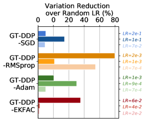
Refer to caption
Figure 8: Variation reduction over 333 different learning rates for each GT-DDP variant on CIFAR-10. We report the value (VARGT-DDP-BaselineVARBaseline)/VARBaselinesubscriptVARGT-DDP-BaselinesubscriptVARBaselinesubscriptVARBaseline(\mathrm{VAR}_{\text{GT-DDP-Baseline}}-\mathrm{VAR}_{\text{Baseline}})/\mathrm{VAR}_{\text{Baseline}}, where each variance is computed over 333 random seeds.