Adaptive Gradient Methods for Constrained Convex Optimization and Variational Inequalities

Abstract

We provide new adaptive first-order methods for constrained convex optimization. Our main algorithms AdaACSA and AdaAGD+ are accelerated methods, which are universal in the sense that they achieve nearly-optimal convergence rates for both smooth and non-smooth functions, even when they only have access to stochastic gradients. In addition, they do not require any prior knowledge on how the objective function is parametrized, since they automatically adjust their per-coordinate learning rate. These can be seen as truly accelerated AdaGrad methods for constrained optimization.

We complement them with a simpler algorithm AdaGrad+ which enjoys the same features, and achieves the standard non-accelerated convergence rate. We also present a set of new results involving adaptive methods for unconstrained optimization and monotone operators.

1 Introduction

Gradient methods are a fundamental building block of modern machine learning. Their scalability and small memory footprint makes them exceptionally well suited to the massive volumes of data used for present-day learning tasks.

While such optimization methods perform very well in practice, one of their major limitations consists of their inability to converge faster by taking advantage of specific features of the input data. For example, the training data used for classification tasks may exhibit a few very informative features, while all the others have only marginal relevance. Having access to this information a priori would enable practitioners to appropriately tune first-order optimization methods, thus allowing them to train much faster. Lacking this knowledge, one may attempt to reach a similar performance by very carefully tuning hyper-parameters, which are all specific to the learning model and input data.

This limitation has motivated the development of adaptive methods, which in absence of prior knowledge concerning the importance of various features in the data, adapt their learning rates based on the information they acquired in previous iterations. The most notable example is AdaGrad (Duchi et al., 2011), which adaptively modifies the learning rate corresponding to each coordinate in the vector of weights. Following its success, a host of new adaptive methods appeared, including Adam (Kingma and Ba, 2014), AmsGrad (Reddi et al., 2018), and Shampoo (Gupta et al., 2018), which attained optimal rates for generic online learning tasks.

A significant series of recent works on adaptive methods addresses the regime of smooth convex functions. Notably, Levy (2017), Cutkosky (2019), Kavis et al. (2019), and Bach and Levy (2019) consider the case of minimizing smooth convex functions without having prior knowledge of the smoothness parameter. While a standard convergence rate of $1/T$ is fairly easily attainable in the case of unconstrained optimization, achieving the optimal $1/T^{2}$ rate becomes significantly more challenging. Even worse, for constrained minimization objectives, where the gradient is nonzero at the optimum, it is generally unclear how an adaptive method can pick the correct step sizes even when aiming for the weaker non-accelerated rate of $1/T$. These difficulties occur when one merely attempts to find the correct learning rate; taking advantage of non-uniform per-coordinate learning rates, as in the case of the original AdaGrad method has remained largely open. In (Kavis et al., 2019), finding such a method with an accelerated $1/T^{2}$ convergence is posed as an open problem, since it would allow the development of robust algorithms that are applicable to non-convex problems such as training deep neural networks.

In this paper, we address this problem and present adaptive algorithms which achieve nearly-optimal convergence with per-coordinate learning rates, even in constrained domains. Our algorithms are universal in the sense that they achieve nearly-optimal convergence rate even when the objective function is non-smooth (Nesterov, 2015). Furthermore, they automatically extend to the case of stochastic optimization, achieving up to logarithmic factors optimal dependence in the standard deviation of the stochastic gradient norm. We complement them with a simpler non-accelerated algorithm which enjoys the same features: it achieves the standard convergence rate on both smooth and non-smooth functions, and does not require prior knowledge of the smoothness parameters, or the variance of the stochastic gradients.

method	non-smooth convergence	smooth convergence
AdaGrad	$O\left(\frac{R_{\infty}\sqrt{d}G}{\sqrt{T}}+\frac{R_{\infty}\sqrt{d}\sigma}{\sqrt{T}}\right)$	$O\left(\frac{R_{\infty}^{2}\sum_{i=1}^{d}\beta_{i}}{T}+\frac{R_{\infty}\sqrt{d}\sigma}{\sqrt{T}}\right)$
	Follows from (Duchi et al., 2011)	Theorem I.3
AdaGrad+	$O\left(\frac{R_{\infty}\sqrt{d}G\sqrt{\ln\left(\frac{GT}{R_{\infty}}\right)}}{\sqrt{T}}+\frac{R_{\infty}\sqrt{d}\sigma\sqrt{\ln\left(\frac{T\sigma}{R_{\infty}}\right)}}{\sqrt{T}}+\frac{R_{\infty}^{2}d}{T}\right)$	$O\left(\frac{R_{\infty}^{2}\sum_{i=1}^{d}\beta_{i}\ln\beta_{i}}{T}+\frac{R_{\infty}\sqrt{d}\sigma\sqrt{\ln\left(\frac{T\sigma}{R_{\infty}}\right)}}{\sqrt{T}}\right)$
	Theorems 3.1, 3.2	Theorems 3.1, 3.2
AdaACSA	$O\left(\frac{R_{\infty}\sqrt{d}G\sqrt{\ln\left(\frac{GT}{R_{\infty}}\right)}+R_{\infty}\sqrt{d}\sigma\sqrt{\ln\left(\frac{T\sigma}{R_{\infty}}\right)}}{\sqrt{T}}+\frac{R_{\infty}^{2}d}{T^{2}}\right)$	$O\left(\frac{R_{\infty}^{2}\sum_{i=1}^{d}\beta_{i}\ln\beta_{i}}{T^{2}}+\frac{R_{\infty}\sqrt{d}\sigma\sqrt{\ln\left(\frac{T\sigma}{R_{\infty}}\right)}}{\sqrt{T}}\right)$
	Theorems 3.3, 3.4	Theorems 3.3, 3.4
AdaAGD+	$O\left(\frac{R_{\infty}\sqrt{d}G\sqrt{\ln\left(\frac{GT}{R_{\infty}}\right)}+R_{\infty}\sqrt{d}\sigma\sqrt{\ln\left(\frac{T\sigma}{R_{\infty}}\right)}}{\sqrt{T}}+\frac{R_{\infty}^{2}d}{T^{2}}\right)$	$O\left(\frac{R_{\infty}^{2}\sum_{i=1}^{d}\beta_{i}\ln\beta_{i}}{T^{2}}+\frac{R_{\infty}\sqrt{d}\sigma\sqrt{\ln\left(\frac{T\sigma}{R_{\infty}}\right)}}{\sqrt{T}}\right)$
	Theorems 3.5, 3.6	Theorems 3.5, 3.6
Adaptive	$O\left(\frac{R_{\infty}\sqrt{d}G\sqrt{\ln\left(\frac{GT}{R_{\infty}}\right)}+R_{\infty}\sqrt{d}\sigma\sqrt{\ln\left(\frac{T\sigma}{R_{\infty}}\right)}}{\sqrt{T}}+\frac{R_{\infty}^{2}d}{T}\right)$	$O\left(\frac{R_{\infty}^{2}\sum_{i=1}^{d}\beta_{i}\ln\beta_{i}}{T}+\frac{R_{\infty}\sqrt{d}\sigma\sqrt{\ln\left(\frac{T\sigma}{R_{\infty}}\right)}}{\sqrt{T}}\right)$
Mirror Prox	Theorem 3.7	Theorem 3.7

Table 1: Convergence rates of adaptive methods in the vector setting. We assume that $f:\mathcal{K}\rightarrow\mathbb{R}$, with $\mathcal{K}\subseteq\mathbb{R}^{d}$, is either smooth with respect to an unknown norm $\left\|\cdot\right\|_{\mathcal{B}}$, where $\mathcal{B}=\textnormal{diag}\left(\beta_{1},\dots,\beta_{d}\right)$, or non-smooth and $G$-Lipschitz. We assume access to stochastic gradients $\widetilde{\nabla}f(x)$ which are unbiased estimators for the true gradient and have bounded variance $\mathbb{E}\left[\left\|\widetilde{\nabla}f(x)-\nabla f(x)\right\|^{2}\right]\leq\sigma^{2}$. The Adaptive Mirror Prox algorithm is for the more general setting of variational inequalities.

Previous Work.

Work on adaptive methods has been extensive, and resulted in a broad range of algorithms (Duchi et al., 2011; Kingma and Ba, 2014; Reddi et al., 2018; Tieleman and Hinton, 2012; Dozat, 2016; Chen et al., 2018). A significant body of work is dedicated to non-convex optimization (Zou et al., 2018; Ward et al., 2019; Zou et al., 2019; Li and Orabona, 2019; Défossez et al., 2020). In a slightly different line of research, there has been recent progress on obtaining improved convergence bounds in the online non-smooth setting; these methods appear in the context of parameter-free optimization, whose main feature is that they adapt to the radius of the domain (Cutkosky and Sarlos, 2019; Cutkosky, 2020).

Here we discuss, for comparison, relevant previous results on adaptive first order methods for smooth convex optimization where the function $f:\mathbb{R}^{d}\rightarrow\mathbb{R}$ to be minimized is smooth with respect to some unknown norm $\left\|\cdot\right\|_{\mathcal{B}}$, where $\mathcal{B}$ is a non-negative diagonal matrix. The case where $\mathcal{B}=\beta I$ is a multiple of the identity corresponds to the standard assumption that $f$ is $\beta$-smooth, and we refer to this as the scalar version of the problem. In the case when $\mathcal{B}$ is a non-negative diagonal matrix, we optimize using the vector version of the problem.

Notably, Levy (2017) presents an adaptive first order method, achieving an optimal convergence rate of $O\left(\beta R^{2}/T\right)$, without requiring prior knowledge of the smoothness $\beta$. While this method also applies to the case where the domain is constrained, it requires the strong condition that the global optimum lies within the domain. In (Levy et al., 2018a), this issue is discussed explicitly, and the line of work is pushed further in the unconstrained case to obtain an accelerated rate of $O\left(\beta R^{2}\ln\left(\beta R/\left\|g_{0}\right\|\right)/T^{2}\right)$, where $g_{0}$ is the gradient evaluated at the initial point. In (Bach and Levy, 2019), the authors consider constrained variational inequalities, which are more general, as they include both convex optimization and convex-concave saddle point problems. The rate they achieve is $O\left(\beta R^{2}/T\right)$, where $\beta$ is the an upper bound on the unknown Lipschitz parameter of the monotone operator, generalizing the case of $\beta$-smooth convex functions. Based on this scheme, in (Kavis et al., 2019) the authors deliver an accelerated adaptive method with nearly optimal rate for the scalar version of the problem. There, they pose as an open problem the question of delivering an accelerated adaptive method for the vector case. We give a more in-depth comparison to previous work in Section A.

Our Contributions.

We give the first adaptive algorithms with per-coordinate step sizes achieving nearly-optimal rates for both constrained convex minimization and variational inequalities arising from monotone operators. Variational inequalities are a very general framework that captures convex minimization, convex-concave saddle point problems, and many other problems of interest (Bach and Levy, 2019; Nemirovski, 2004). Our algorithms are universal, in the sense defined by Nesterov (2015). They automatically achieve optimal convergence rates (up to a $\sqrt{\ln T}$ factor) in the smooth and non-smooth setting, both in the deterministic setting as well as the stochastic setting where we have access to noisy gradient or operator evaluations. Our algorithms automatically adapt to problem parameters such as smoothness, gradient or operator norms, and the variance of the stochastic gradient or operator norms. Our results answer several open questions raised in previous work (Kavis et al., 2019; Bach and Levy, 2019).

For constrained convex minimization, we present three algorithms: AdaGrad+, AdaACSA, and AdaAGD+. For $\beta$-smooth functions, AdaGrad+ convergences at the rate $O\left(R_{\infty}^{2}d\cdot\beta\ln\beta/T\right)$, and AdaACSA and AdaAGD+ converge at the rate $O\left(R_{\infty}^{2}d\cdot\beta\ln\beta/T^{2}\right)$. Since $R_{\infty}d^{1/2}$ is the $\ell_{2}$ diameter of the region containing the $\ell_{\infty}$ ball of radius $R_{\infty}$, these exactly match the rates of standard non-accelerated and accelerated gradient decent, when the domain is an $\ell_{\infty}$ ball (Nesterov, 2013). Therefore these schemes can be interpreted as learning the optimal diagonal preconditioner for a smooth function $f$.

For variational inequalities, we present the Adaptive Mirror Prox algorithm that couples the Universal Mirror-Prox scheme (Bach and Levy, 2019; Nemirovski, 2004) with novel per-coordinate step sizes. The Universal Mirror-Prox algorithm of Bach and Levy (2019) sets a single step size for all coordinates that is initialized using an estimate for the gradient norms. In contrast, our algorithm uses per-coordinate step sizes that are initialized to an absolute constant. In addition to eliminating a hyperparameter that we would need to tune, this approach leads to larger stepsizes. Adaptive methods such as AdaGrad are also implemented and used in practice using step sizes initialized to a small constant, such as $\epsilon=10^{-10}$. We show that the algorithm simultaneously achieves convergence guarantees that are optimal (up to a $\sqrt{\ln T}$ factor) for both smooth and non-smooth operators, as well as in the deterministic and stochastic settings.

Algorithmically, we provide a new rule for updating the diagonal preconditioner, which is better suited to constrained optimization. While the unconstrained AdaGrad algorithm updates the preconditioner based on the previously seen gradients, here we update based on the movement performed by the iterate (see Figure 1). In the unconstrained setting, our update rule matches the standard AdaGrad update. The works (Kavis et al., 2019; Joulani et al., 2020) tackled the difficulties introduced by constraining the domain by using a different update rule based on the change in gradients.

Contemporaneous Work.

Joulani et al. (2020) also obtain an accelerated algorithm with coordinate-wise adaptive rates, in constrained domains. The convergence guarantee is stronger than ours by a $O(\ln\beta)$ factor in the smooth setting, where $\beta$ is the smoothness constant, and by a $O(\sqrt{\ln T})$ factor in the non-smooth and stochastic settings. On the other hand, we obtain adaptive schemes for a wide-range of settings, including a non-dual-averaging scheme ($\text{$\textsc{AdaACSA}$},$ based on the AC-SA algorithm (Lan, 2012)), a dual-averaging scheme (AdaAGD+, based on the AGD+ algorithm (Cohen et al., 2018)), and an adaptive mirror-prox scheme (Bach and Levy, 2019; Nemirovski, 2004) for solving variational inequalities which generalizes both convex minimization and convex-concave zero-sum games. The latter answers an open question (Bach and Levy, 2019). Joulani et al. (2020) propose a very different dual-averaging scheme for convex minimization based on the online-to-batch conversion (Cutkosky, 2019; Kavis et al., 2019) and the online learning with optimism framework (Mohri and Yang, 2016). Our algorithms use the iterate movement to set the per-coordinate step sizes, whereas the algorithm presented in (Joulani et al., 2020) uses the change in gradients.

Roadmap

The rest of the paper is organized as follows.

Section 2	We introduce relevant notation and concepts.
Section 3	We present our adaptive schemes for constrained convex minimization $(\textsc{AdaGrad+}$, AdaACSA, AdaAGD+) and variational inequalities (Adaptive Mirror Prox), and state their convergence guarantees.
Section 4	We analyze the convergence of AdaGrad+ for smooth functions in the deterministic setting.
Section 5	We analyze the convergence of AdaACSA for smooth functions in the deterministic setting.
Section A	We present the scalar versions of our schemes, provide their convergence guarantees, and discuss their relation to previous work.
Section B	We analyze the convergence of AdaGrad+ for non-smooth functions in the deterministic setting.
Section C	We analyze the convergence of AdaGrad+ for both smooth and non-smooth functions in the stochastic setting.
Section D	We analyze the convergence of AdaACSA for non-smooth functions in the deterministic setting.
Section E	We analyze the convergence of AdaACSA for both smooth and non-smooth functions in the stochastic setting.
Section F	We analyze the convergence of AdaAGD+ for smooth functions in the deterministic setting.
Section G	We analyze the convergence of AdaAGD+ for non-smooth functions in the deterministic setting.
Section H	We analyze the convergence of AdaAGD+ for both smooth and non-smooth functions in the stochastic setting.
Section I	We extend the analysis of Levy et al. (2018a) to the vector setting, and obtain a sharp analysis for the standard AdaGrad algorithm for smooth functions in the unconstrained setting (Theorem I.1), which saves the extra logarithmic factors that AdaGrad+ pays in constrained domains. We also provide its guarantees in the stochastic setup (Theorem I.3).
Section J	We extend the universal mirror prox method of Bach and Levy (2019) to the vector setting, and resolve the open question asked by them.
Section K	We provide experimental results.

2 Preliminaries

Constrained Convex Optimization.

We consider the problem $\min_{x\in\mathcal{K}}f(x)$, where $f\colon\mathbb{R}^{d}\to\mathbb{R}$ is a convex function and $\mathcal{K}\subseteq\mathbb{R}^{d}$ is an arbitrary convex set. For simplicity, we assume that $f$ is continuously differentiable and we let $\nabla f(x)$ denote the gradient of $f$ at $x$. We assume access to projections over $\mathcal{K}$ in the sense that we can efficiently solve problems of the form $\arg\min_{x\in\mathcal{K}}\left\langle g,x\right\rangle+\frac{1}{2}\left\|x\right\|_{D}^{2}$, where $D$ is an arbitrary non-negative diagonal matrix and $\left\|x\right\|_{D}=\sqrt{x^{\top}Dx}$.

We say that $f$ is smooth with respect to the norm $\left\|\cdot\right\|_{\mathcal{B}}$ if $\nabla^{2}f(x)\preceq\mathcal{B}$, for all $x\in\mathcal{K}$. Equivalently, we have $f(y)\leq f(x)+\left\langle\nabla f(x),y-x\right\rangle+\frac{1}{2}\left\|x-y\right\|_{\mathcal{B}}^{2}$ , for all $x,y\in\mathcal{K}$. We say that $f$ is strongly convex with respect to the norm $\left\|\cdot\right\|_{\mathcal{B}}$ if $\nabla^{2}f(x)\succeq\mathcal{B}$, for all $x\in\mathcal{K}$.

Variational Inequalities.

We also consider the more general problem setting of variational inequalities arising from monotone operators. Let $\mathcal{K}\subseteq\mathbb{R}^{d}$ be a convex set and let $F\colon\mathcal{K}\to\mathbb{R}^{d}$ be an operator. The operator $F$ is monotone if it satisfies $\left\langle F(x)-F(y),x-y\right\rangle\geq 0$ for all $x,y\in\mathcal{K}$ and it is smooth with respect to the norm $\left\|\cdot\right\|_{\mathcal{B}}$ if $\left\|F(x)-F(y)\right\|_{\mathcal{B}^{-1}}\leq\left\|x-y\right\|_{\mathcal{B}}$ for all $x,y\in\mathcal{K}$. The goal is to find a strong solution $x^{*}$ for the variational inequality arising from $F$, i.e., a solution $x^{*}\in\mathcal{K}$ satisfying $\left\langle F(x^{*}),x^{*}-x\right\rangle\leq 0$ for all $x\in\mathcal{K}$. Variational inequalities are a very general framework that captures convex minimization, convex-concave saddle point problems, and many other problems of interest (Bach and Levy, 2019; Nemirovski, 2004). For convex minimization, the operator $F(x)$ is simply the gradient $\nabla f(x)$.

Notation.

For diagonal matrices $D$, we use $D_{i}$ to refer to the $i^{th}$ diagonal entry. We use $R$ to denote the $\ell_{2}$ diameter of the domain $\mathcal{K}$, $R=\max_{x,y\in\mathcal{K}}\left\|x-y\right\|_{2}$, and similarly $R_{\infty}$ to denote the $\ell_{\infty}$ diameter of $\mathcal{K}$. When the function is not continuously differentiable, we abuse notation and use $\nabla f(x)$ to denote a subgradient of $f$ at $x$. We use $G$ to denote the Lipschitz constant of $f$ i.e. $G=\max_{x\in\mathcal{K}}\left\|\nabla f(x)\right\|_{2}$. In the stochastic setting, our algorithms assume access to gradient estimators $\widetilde{\nabla}f(x)$ satisfying the following standard assumptions for a fixed (but unknown) scalar $\sigma$:

$$\mathbb{E}\left[\widetilde{\nabla}f(x)|x\right] =\nabla f(x)\ ,$$ (1)

$$\mathbb{E}\left[\left\|\widetilde{\nabla}f(x)-\nabla f(x)\right\|^{2}\right] \leq\sigma^{2}\ .$$ (2)

3 Adaptive Schemes for Constrained Convex Optimization and Variational Inequalities

In this section, we present our algorithms for constrained convex minimization and variational inequalities.

3.1 Constrained AdaGrad Scheme

Let $x_{0}\in\mathcal{K}$, $D_{0}=I$, $R_{\infty}\geq\max_{x,y\in\mathcal{K}}\left\|x-y\right\|_{\infty}$. For $t=0,\dots,T-1$, update: $\displaystyle x_{t+1}=$ $\displaystyle\arg\min_{x\in\mathcal{K}}\left\{\left\langle\nabla f(x_{t}),x\right\rangle+\frac{1}{2}\left\|x-x_{t}\right\|_{D_{t}}^{2}\right\}\ ,$ $\displaystyle D_{t+1,i}^{2}$ $\displaystyle=D_{t,i}^{2}\left(1+\frac{\left(x_{t+1,i}-x_{t,i}\right)^{2}}{R_{\infty}^{2}}\right)\ ,\text{for all }i\in[d].$ Return $\overline{x}_{T}=\frac{1}{T}\sum_{t=1}^{T}x_{t}$.

Figure 1: AdaGrad+ algorithm.

Figure 1 shows our AdaGrad+ algorithm for constrained convex optimization. The algorithm can be viewed as a generalization of the celebrated AdaGrad algorithm of Duchi et al. (2011) to the constrained setting where the feasible set $\mathcal{K}$ is an arbitrary convex set. To see the parallel with AdaGrad, consider the gradient mapping:

$$g_{t}=-D_{t}\left(x_{t+1}-x_{t}\right)\Leftrightarrow x_{t+1}=x_{t}-D_{t}^{-1}g_{t}\ .$$

Letting $\eta=R_{\infty}$, the update is

$$x_{t+1,i} =x_{t,i}-\frac{\eta}{\sqrt{\eta^{2}+\sum_{s=1}^{t-1}g_{s,i}^{2}}}g_{t,i}\ , \forall i\in[d]\ .$$

In the unconstrained setting, we have $g_{t}=\nabla f(x_{t})$ and our scheme almost coincides with AdaGrad. We have chosen the initial scaling to be the identity, whereas the original AdaGrad scheme uses $D_{0}=\epsilon I$. Our analysis extends to this choice and we incur an additional $O\left(\ln(1/\epsilon)\right)$ factor in the convergence guarantee. In addition, the diagonal matrix $D_{t}$ we use is off by one iterate, in the sense that it does not contain information about $g_{t}$. This is an essential feature of our method, since in the constrained setting computing the gradient mapping requires access to $D_{t}$.

Similarly to (Bach and Levy, 2019), we can motivate the choice of updating $D$ by the iterate movement as follows. The algorithm simultaneously addresses the unconstrained setting and the more challenging constrained setting. Since our goal is to design a universal method, intuitively we would like the step size to decay in the non-smooth setting and to remain constant in the smooth setting, similarly to the standard (non-adaptive) gradient descent schemes. In the unconstrained setting, the iterate movement coincides with the gradient. In the constrained setting, the gradient is non-zero at the optimum and we cannot hope that the gradient norm decreases as we approach the optimum. Instead, as the iterate converges to the optimum, the movement also goes to zero and thus our adaptive step size remains around the optimal value.

Covergence Guarantees for AdaGrad+.

We show that the algorithm is universal and it obtains the smooth rate of $\frac{1}{T}$ if the function is smooth while retaining the optimal $\frac{1}{\sqrt{T}}$ rate if the function is non-smooth. The algorithm automatically adapts to the smoothness parameters, the gradient norm, and the variance parameter. The following theorem states the precise convergence guarantees in the deterministic setting.

Theorem 3.1.

Let $x^{*}\in\arg\min_{x\in\mathcal{K}}f(x)$, $R_{\infty}\geq\max_{x,y\in\mathcal{K}}\left\|x-y\right\|_{\infty}$, $G\geq\max_{x\in\mathcal{K}}\left\|\nabla f(x)\right\|_{2}$, Let $x_{t}$ be the iterates constructed by the algorithm in Figure 1 and let $\overline{x}_{T}=\frac{1}{T}\sum_{t=0}^{T-1}x_{t}$. If $f$ is a convex function, we have

$$f(\overline{x}_{T})-f(x^{*})\leq O\left(\frac{R_{\infty}\sqrt{d}G\sqrt{\ln\left(\frac{GT}{R_{\infty}}\right)}}{\sqrt{T}}+\frac{R_{\infty}^{2}d}{T}\right)\ .$$

If $f$ is additionally $1$-smooth with respect to the norm $\left\|\cdot\right\|_{\mathcal{B}}$, where $\mathcal{B}=\textnormal{diag}(\beta_{1},\dots,\beta_{d})$ is a diagonal matrix with $\beta_{1},\dots,\beta_{d}\geq 1$, we have

$$f(\overline{x}_{T})-f(x^{*})\leq O\left(\frac{R_{\infty}^{2}\sum_{i=1}^{d}\beta_{i}\ln\left(2\beta_{i}\right)}{T}\right)\ .$$

In Section C, we extend the algorithm and its analysis to the stochastic setting where we are given stochastic gradients $\widetilde{\nabla}f(x)$ satisfying the assumptions (1) and (2). The following theorem state the precise convergence guarantees in the stochastic setting.

Theorem 3.2.

Let $x^{*}\in\arg\min_{x\in\mathcal{K}}f(x)$, $R_{\infty}\geq\max_{x,y\in\mathcal{K}}\left\|x-y\right\|_{\infty}$, $G\geq\max_{x\in\mathcal{K}}\left\|\nabla f(x)\right\|_{2}$, and $\sigma^{2}$ be the variance of the stochastic gradients ((1) and (2)). Let $x_{t}$ be the iterates constructed by the algorithm in Figure 8 and let $\overline{x}_{T}=\frac{1}{T}\sum_{t=0}^{T-1}x_{t}$. If $f$ is a convex function, we have

$$\mathbb{E}\left[f(\overline{x}_{T})-f(x^{*})\right]\leq O\left(\frac{R_{\infty}\sqrt{d}G\sqrt{\ln\left(\frac{GT}{R_{\infty}}\right)}}{\sqrt{T}}+\frac{R_{\infty}\sqrt{d}\sigma\sqrt{\ln\left(\frac{T\sigma}{R_{\infty}}\right)}}{\sqrt{T}}+\frac{R_{\infty}^{2}d}{T}\right)\ .$$

If $f$ is additionally $1$-smooth with respect to the norm $\left\|\cdot\right\|_{\mathcal{B}}$, where $\mathcal{B}=\textnormal{diag}(\beta_{1},\dots,\beta_{d})$ is a diagonal matrix with $\beta_{1},\dots,\beta_{d}\geq 1$, we have

$$\mathbb{E}\left[f(\overline{x}_{T})-f(x^{*})\right]\leq O\left(\frac{R_{\infty}^{2}\sum_{i=1}^{d}\beta_{i}\ln\left(2\beta_{i}\right)}{T}+\frac{R_{\infty}\sigma\sqrt{d\ln\left(\frac{T\sigma}{R_{\infty}}\right)}}{\sqrt{T}}\right)\ .$$

In Sections 4 and B, we analyze the algorithm in the deterministic setting where we have access to the actual gradients ($\sigma=0$). We extend the analysis to the stochastic setting in Section C. We note that we have $D_{t+1,i}^{2}\leq 2D_{t,i}^{2}$. This property will play an important role in our analysis.

3.2 Accelerated Schemes

We give two adaptive schemes for constrained convex optimization that achieve the optimal rate of $\frac{1}{T^{2}}$ for smooth functions without knowing the smoothness parameters. Our algorithms are adaptive versions of the AC-SA algorithm (Lan, 2012), and the AGD+ algorithm (Cohen et al., 2018). For this reason, we coin the names AdaACSA (Figure 2) and AdaAGD+ (Figure 3). The AGD+ algorithm is a dual-averaging version of AC-SA. The algorithms and their adaptive versions have different iterates and they may be useful in different contexts.

We show that our algorithms simultaneously achieve convergence rates that are optimal (up to a $\sqrt{\ln T}$ factor) for both smooth and non-smooth functions, both in the deterministic and stochastic setting. The algorithms automatically adapt to the smoothness parameters, the gradient norm, and the variance parameter.

Let $D_{0}=I$, $z_{0}\in\mathcal{K}$, $\alpha_{t}=\gamma_{t}=1+\frac{t}{3}$, $R_{\infty}^{2}\geq\max_{x,y\in\mathcal{K}}\left\|x-y\right\|_{\infty}^{2}$. For $t=0,\dots,T-1$, update: $\displaystyle x_{t}$ $\displaystyle=\left(1-\alpha_{t}^{-1}\right)y_{t}+\alpha_{t}^{-1}z_{t}\ ,$ $\displaystyle z_{t+1}$ $\displaystyle=\arg\min_{u\in\mathcal{K}}\left\{\gamma_{t}\left\langle\nabla f(x_{t}),u\right\rangle+\frac{1}{2}\left\|u-z_{t}\right\|_{D_{t}}^{2}\right\}\ ,$ $\displaystyle y_{t+1}$ $\displaystyle=\left(1-\alpha_{t}^{-1}\right)y_{t}+\alpha_{t}^{-1}z_{t+1}\ ,$ $\displaystyle D_{t+1,i}^{2}$ $\displaystyle=D_{t,i}^{2}\left(1+\frac{\left(z_{t+1,i}-z_{t,i}\right)^{2}}{R_{\infty}^{2}}\right)\ ,\text{for all }i\in[d].$ Return $y_{T}$.

Figure 2: AdaACSA algorithm.

Convergence Guarantees for AdaACSA.

We show that AdaACSA is universal and it simultaneously achieves the optimal convergence rate for both smooth and non-smooth optimization. The following theorem states the precise convergence guarantees in the deterministic setting.

Theorem 3.3.

Let $x^{*}\in\arg\min_{x\in\mathcal{K}}f(x)$, $R_{\infty}\geq\max_{x,y\in\mathcal{K}}\left\|x-y\right\|_{\infty}$, $G\geq\max_{x\in\mathcal{K}}\left\|\nabla f(x)\right\|_{2}$. Let $y_{t}$ be the iterates constructed by the algorithm in Figure 2. If $f$ is a convex function, we have

$$f(y_{T})-f(x^{*}) \leq O\left(\frac{R_{\infty}\sqrt{d}G\sqrt{\ln\left(\frac{GT}{R_{\infty}}\right)}}{\sqrt{T}}+\frac{R_{\infty}^{2}d}{T^{2}}\right)\ .$$

If $f$ is additionally $1$-smooth with respect to the norm $\left\|\cdot\right\|_{\mathcal{B}}$, where $\mathcal{B}=\textnormal{diag}(\beta_{1},\dots,\beta_{d})$ is a diagonal matrix with $\beta_{1},\dots,\beta_{d}\geq 1$, we have

$$f(y_{T})-f(x^{*})\leq O\left(\frac{R_{\infty}^{2}\sum_{i=1}^{d}\beta_{i}\ln\left(2\beta_{i}\right)}{T^{2}}\right)\ .$$

In Section E, we extend the AdaACSA algorithm and its analysis to the stochastic setting where we are given stochastic gradients $\widetilde{\nabla}f(x)$ satisfying the assumptions (1) and (2). The following theorem state the precise convergence guarantees in the stochastic setting.

Theorem 3.4.

Let $x^{*}\in\arg\min_{x\in\mathcal{K}}f(x)$, $R_{\infty}\geq\max_{x,y\in\mathcal{K}}\left\|x-y\right\|_{\infty}$, $G\geq\max_{x\in\mathcal{K}}\left\|\nabla f(x)\right\|_{2}$, and $\sigma^{2}$ be the variance of the stochastic gradients ((1) and (2)). Let $y_{t}$ be the iterates constructed by the algorithm in Figure 9. If $f$ is a convex function, we have

$$\mathbb{E}\left[f(y_{T})-f(x^{*})\right] \leq O\left(\frac{R_{\infty}\sqrt{d}G\sqrt{\ln\left(\frac{GT}{R_{\infty}}\right)}+R_{\infty}\sqrt{d}\sigma\sqrt{\ln\left(\frac{T\sigma}{R_{\infty}}\right)}}{\sqrt{T}}+\frac{R_{\infty}^{2}d}{T^{2}}\right)\ .$$

If $f$ is additionally $1$-smooth with respect to the norm $\left\|\cdot\right\|_{\mathcal{B}}$, where $\mathcal{B}=\textnormal{diag}(\beta_{1},\dots,\beta_{d})$ is a diagonal matrix with $\beta_{1},\dots,\beta_{d}\geq 1$, we have

$$\mathbb{E}\left[f(y_{T})-f(x^{*})\right]\leq O\left(\frac{R_{\infty}^{2}\sum_{i=1}^{d}\beta_{i}\ln\left(2\beta_{i}\right)}{T^{2}}+\frac{R_{\infty}\sqrt{d}\sigma\sqrt{\ln\left(\frac{T\sigma}{R_{\infty}}\right)}}{\sqrt{T}}\right)\ .$$

In Sections 5 and D, we analyze the AdaACSA algorithm in the deterministic setting where we have access to the actual gradients ($\sigma=0$). We extend the analysis to the stochastic setting in Section E.

Let $D_{1}=I$, $z_{0}\in\mathcal{K}$, $a_{t}=t$, $A_{t}=\sum_{i=1}^{t}a_{i}=\frac{t(t+1)}{2}$, $R_{\infty}^{2}\geq\max_{x,y\in\mathcal{K}}\left\|x-y\right\|_{\infty}^{2}$. For $t=1,\dots,T$, update: $\displaystyle x_{t}$ $\displaystyle=\frac{A_{t-1}}{A_{t}}y_{t-1}+\frac{a_{t}}{A_{t}}z_{t-1}\ ,$ $\displaystyle z_{t}$ $\displaystyle=\arg\min_{u\in\mathcal{K}}\left(\sum_{i=1}^{t}\left\langle a_{i}\nabla f(x_{i}),u\right\rangle+\frac{1}{2}\left\|u-z_{0}\right\|_{D_{t}}^{2}\right)$ $\displaystyle y_{t}$ $\displaystyle=\frac{A_{t-1}}{A_{t}}y_{t-1}+\frac{a_{t}}{A_{t}}z_{t}\ ,$ $\displaystyle D_{t+1,i}^{2}$ $\displaystyle=D_{t,i}^{2}\left(1+\frac{\left(z_{t,i}-z_{t-1,i}\right)^{2}}{R_{\infty}^{2}}\right)\ ,\text{for all }i\in[d].$ Return $y_{T}$.

Figure 3: AdaAGD+ algorithm.

Convergence Guarantees for AdaAGD+.

We show that AdaAGD+ is universal and it simultaneously achieves the optimal convergence rate for both smooth and non-smooth optimization. The following theorem states the precise convergence guarantees in the deterministic setting.

Theorem 3.5.

Let $x^{*}\in\arg\min_{x\in\mathcal{K}}f(x)$, $R_{\infty}\geq\max_{x,y\in\mathcal{K}}\left\|x-y\right\|_{\infty}$, $G\geq\max_{x\in\mathcal{K}}\left\|\nabla f(x)\right\|_{2}$. Let $y_{t}$ be the iterates constructed by the algorithm in Figure 3. If $f$ is a convex function, we have

$$f(y_{T})-f(x^{*}) \leq O\left(\frac{R_{\infty}\sqrt{d}G\sqrt{\ln\left(\frac{GT}{R_{\infty}}\right)}}{\sqrt{T}}+\frac{R_{\infty}^{2}d}{T^{2}}\right)\ .$$

If $f$ is additionally $1$-smooth with respect to the norm $\left\|\cdot\right\|_{\mathcal{B}}$, where $\mathcal{B}=\textnormal{diag}(\beta_{1},\dots,\beta_{d})$ is a diagonal matrix with $\beta_{1},\dots,\beta_{d}\geq 1$, we have

$$f(y_{T})-f(x^{*})\leq O\left(\frac{R_{\infty}^{2}\sum_{i=1}^{d}\beta_{i}\ln\left(2\beta_{i}\right)}{T^{2}}\right)\ .$$

In Section H, we extend the AdaAGD+ algorithm and its analysis to the stochastic setting where we are given stochastic gradients $\widetilde{\nabla}f(x)$ satisfying the assumptions (1) and (2). The following theorem state the precise convergence guarantees in the stochastic setting.

Theorem 3.6.

Let $x^{*}\in\arg\min_{x\in\mathcal{K}}f(x)$, $R_{\infty}\geq\max_{x,y\in\mathcal{K}}\left\|x-y\right\|_{\infty}$, $G\geq\max_{x\in\mathcal{K}}\left\|\nabla f(x)\right\|_{2}$, and $\sigma^{2}$ be the variance of the stochastic gradients ((1) and (2)). Let $y_{t}$ be the iterates constructed by the algorithm in Figure 10. If $f$ is a convex function, we have

$$\mathbb{E}\left[f(y_{T})-f(x^{*})\right] \leq O\left(\frac{R_{\infty}\sqrt{d}G\sqrt{\ln\left(\frac{GT}{R_{\infty}}\right)}+R_{\infty}\sqrt{d}\sigma\sqrt{\ln\left(\frac{T\sigma}{R_{\infty}}\right)}}{\sqrt{T}}+\frac{R_{\infty}^{2}d}{T^{2}}\right)\ .$$

If $f$ is additionally $1$-smooth with respect to the norm $\left\|\cdot\right\|_{\mathcal{B}}$, where $\mathcal{B}=\textnormal{diag}(\beta_{1},\dots,\beta_{d})$ is a diagonal matrix with $\beta_{1},\dots,\beta_{d}\geq 1$, we have

$$\mathbb{E}\left[f(y_{T})-f(x^{*})\right]\leq O\left(\frac{R_{\infty}^{2}\sum_{i=1}^{d}\beta_{i}\ln\left(2\beta_{i}\right)}{T^{2}}+\frac{R_{\infty}\sqrt{d}\sigma\sqrt{\ln\left(\frac{T\sigma}{R_{\infty}}\right)}}{\sqrt{T}}\right)\ .$$

In Sections F and G, we analyze the algorithm in the deterministic setting where we have access to the actual gradients ($\sigma=0$). We extend the analysis to the stochastic setting in Section H.

3.3 Variational Inequalities

Building on the work of Bach and Levy (2019), we give the first universal method with per-coordinate adaptive step sizes for variational inequalities arising from monotone operators, and answer the open question asked by them. The algorithm, shown in Figure 4, is the natural extension to the vector setting of the scheme of Bach and Levy (2019). A notable difference is that the algorithm provided in (Bach and Levy, 2019) uses an estimate for $G\geq\max_{x\in\mathcal{K}}\left\|F(x)\right\|$ as part of the step size. Our algorithm does not use the $G$ parameter and it automatically adapts to it, as well as the smoothness and variance parameters.

Let $y_{0}\in\mathcal{K}$, $D_{1}=I$, $R_{\infty}\geq\max_{x,y\in K}\left\|x-y\right\|_{\infty}$. For $t=1,\dots,T$, update: $\displaystyle x_{t}$ $\displaystyle=\arg\min_{x\in\mathcal{K}}\left\{\left\langle F(y_{t-1}),x\right\rangle+\frac{1}{2}\left\|x-y_{t-1}\right\|_{D_{t}}^{2}\right\}\ ,$ $\displaystyle y_{t}$ $\displaystyle=\arg\min_{x\in\mathcal{K}}\left\{\left\langle F(x_{t}),x\right\rangle+\frac{1}{2}\left\|x-y_{t-1}\right\|_{D_{t}}^{2}\right\}\ ,$ $\displaystyle D_{t+1,i}^{2}$ $\displaystyle=D_{t,i}^{2}\left(1+\frac{\left(x_{t,i}-y_{t-1,i}\right)^{2}+\left(x_{t,i}-y_{t,i}\right)^{2}}{2R_{\infty}^{2}}\right)\ .$ Return $\overline{x}_{T}=\frac{1}{T}\sum_{t=1}^{T}x_{t}$.

Figure 4: Adaptive Mirror Prox algorithm, extending Bach and Levy (2019) to the vector setting.

Convergence Guarantees for Adaptive Mirror Prox.

By combining the analysis of Bach and Levy (2019) with our techniques from the other sections, we show that the algorithm is universal and it simultaneously achieves the nearly-optimal rates (up to a $\sqrt{\ln T}$ factor) for both smooth and non-smooth operators. The following theorem shows the precise convergence guarantees in the deterministic setting ($\sigma=0$), and we give the proof in Section J. We refer the reader to Section J for the precise definitions which concern this setting.

Theorem 3.7.

Consider the problem $\min_{x\in\mathcal{K}}F(x)$, where $F$ is a monotone operator and $\mathcal{K}$ is a convex set. Let $R_{\infty}\geq\max_{x,y\in K}\left\|x-y\right\|_{\infty}$ and $G\geq\max_{x\in\mathcal{K}}\left\|F(x)\right\|_{2}$ . Let $x_{t}$ be the iterates constructed by the algorithm in Figure 4 and let $\overline{x}_{T}=\frac{1}{T}\sum_{t=1}^{T}x_{t}$. We have

$$\textnormal{DualityGap}(\overline{x}_{T})\leq O\left(\frac{\sqrt{d}R_{\infty}G\sqrt{\ln\left(\frac{GT}{R_{\infty}}\right)}}{\sqrt{T}}+\frac{R_{\infty}^{2}d}{T}\right)\ .$$

If $F$ is additionally $1$-smooth with respect to the norm $\left\|\cdot\right\|_{\mathcal{B}}$, where $\mathcal{B}=\textnormal{diag}(\beta_{1},\dots,\beta_{d})$ is a diagonal matrix with $\beta_{1},\dots,\beta_{d}\geq 1$, we have

$$\textnormal{DualityGap}(\overline{x}_{T})\leq O\left(\frac{R_{\infty}^{2}\sum_{i=1}^{d}\beta_{i}\ln\left(2\beta_{i}\right)}{T}\right)\ .$$

Extension to the stochastic setting.

Analogously to our other results, in the stochastic setting, we assume that we are given noisy evaluations $\widetilde{F}(x_{t})$ satisfying the expectation and variance assumptions $\mathbb{E}\left[\widetilde{F}(x_{t})|x_{t}\right]=F(x_{t})$ and $\mathbb{E}\left[\left\|\widetilde{F}(x_{t})-F(x_{t})\right\|^{2}\right]\leq\sigma^{2}$. The algorithm and its analysis can be easily extended to the stochastic setting using the techniques developed in Sections C, E and H, and we omit this straightforward extension. We refer the reader to 1 for the convergence guarantee in the stochastic setting.

We note that, in the sthocastic setting, the analysis of Bach and Levy (2019) makes the additional assumption that the stochastic values have bounded norms almost surely, i.e., $\left\|\widetilde{F}(x_{t})\right\|\leq G$ with probability one, which is stronger than our assumption of bounded variance. This assumption simplifies the analysis, as it allows one to directly upper bound $D_{T}$ (equivalently, lower bound the step size $\eta_{T}=1/D_{T}$), which is the key loss term in the convergence analysis. Our analysis removes this assumption by employing a more involved argument that does not upper bound $\text{Tr}(D_{T})$ directly.

4 Analysis of AdaGrad+ for Smooth Functions

We make the following observation that will be used in the analysis: we have $D_{t+1,i}^{2}\leq 2D_{t,i}^{2}$ for all iterations $t\in[T]$ and coordinates $i\in[d]$. We start with the following lemma, which follows from the standard analysis of gradient descent.

Lemma 4.1.

For any $y\in\mathcal{K}$, we have

$$f(x_{t+1})-f(y) \leq\left\langle D_{t}\left(x_{t}-x_{t+1}\right),x_{t}-y\right\rangle-\left\|x_{t+1}-x_{t}\right\|_{D_{t}}^{2}+\frac{1}{2}\left\|x_{t+1}-x_{t}\right\|_{\mathcal{B}}^{2}$$

$$=\frac{1}{2}\left(\left\|x_{t}-y\right\|_{D_{t}}^{2}-\left\|x_{t+1}-y\right\|_{D_{t}}^{2}-\left\|x_{t+1}-x_{t}\right\|_{D_{t}}^{2}\right)+\frac{1}{2}\left\|x_{t+1}-x_{t}\right\|_{\mathcal{B}}^{2}\ .$$

Proof.

We write $f(x_{t+1})-f(y)=f(x_{t+1})-f(x_{t})+f(x_{t})-f(y)$, and we use smoothness to bound the first term and convexity to bound the second term.

$$f(x_{t+1})-f(y) =f(x_{t+1})-f(x_{t})+f(x_{t})-f(y)$$

$$\leq\left\langle\nabla f(x_{t}),x_{t+1}-x_{t}\right\rangle+\frac{1}{2}\left\|x_{t+1}-x_{t}\right\|_{\mathcal{B}}^{2}+\left\langle\nabla f(x_{t}),x_{t}-y\right\rangle$$

$$=\left\langle\nabla f(x_{t}),x_{t+1}-y\right\rangle+\frac{1}{2}\left\|x_{t+1}-x_{t}\right\|_{\mathcal{B}}^{2}\ .$$

Next, we use the first-order optimality condition for $x_{t+1}$ to obtain

$$\left\langle\nabla f(x_{t})+D_{t}\left(x_{t+1}-x_{t}\right),x_{t+1}-y\right\rangle\leq 0\ .$$

By rearranging, we obtain

$$\left\langle\nabla f(x_{t}),x_{t+1}-y\right\rangle \leq\left\langle D_{t}\left(x_{t}-x_{t+1}\right),x_{t+1}-y\right\rangle$$

$$=\left\langle D_{t}\left(x_{t}-x_{t+1}\right),x_{t}-y+x_{t+1}-x_{t}\right\rangle$$

$$=\left\langle D_{t}\left(x_{t}-x_{t+1}\right),x_{t}-y\right\rangle-\left\|x_{t+1}-x_{t}\right\|_{D_{t}}^{2}\ .$$

Plugging into the previous inequality gives

$$f(x_{t+1})-f(y) \leq\left\langle D_{t}\left(x_{t}-x_{t+1}\right),x_{t}-y\right\rangle-\left\|x_{t+1}-x_{t}\right\|_{D_{t}}^{2}+\frac{1}{2}\left\|x_{t+1}-x_{t}\right\|_{\mathcal{B}}^{2}\ .$$

Finally, we note that

$$\left\langle D_{t}\left(x_{t}-x_{t+1}\right),x_{t}-y\right\rangle=\frac{1}{2}\left(\left\|x_{t}-y\right\|_{D_{t}}^{2}-\left\|x_{t+1}-y\right\|_{D_{t}}^{2}+\left\|x_{t+1}-x_{t}\right\|_{D_{t}}^{2}\right)\ .$$

Indeed, we have

$$\left\|x_{t}-y\right\|_{D_{t}}^{2}-\left\|x_{t+1}-y\right\|_{D_{t}}^{2}+\left\|x_{t+1}-x_{t}\right\|_{D_{t}}^{2}$$

$$=\left\|x_{t}-x_{t+1}+x_{t+1}-y\right\|_{D_{t}}^{2}-\left\|x_{t+1}-y\right\|_{D_{t}}^{2}+\left\|x_{t+1}-x_{t}\right\|_{D_{t}}^{2}$$

$$=2\left\|x_{t}-x_{t+1}\right\|_{D_{t}}^{2}+2\left\langle D_{t}\left(x_{t}-x_{t+1}\right),x_{t+1}-y\right\rangle$$

$$=2\left\|x_{t}-x_{t+1}\right\|_{D_{t}}^{2}+2\left\langle D_{t}\left(x_{t}-x_{t+1}\right),x_{t+1}-x_{t}+x_{t}-y\right\rangle$$

$$=2\left\|x_{t}-x_{t+1}\right\|_{D_{t}}^{2}-2\left\|x_{t+1}-x_{t}\right\|_{D_{t}}^{2}+2\left\langle D_{t}\left(x_{t}-x_{t+1}\right),x_{t}-y\right\rangle$$

$$=2\left\langle D_{t}\left(x_{t}-x_{t+1}\right),x_{t}-y\right\rangle\ .$$

∎

Using the standard AdaGrad analysis, we obtain the following lemma.

Lemma 4.2.

We have

$$\sum_{t=0}^{T-1}\left(f(x_{t+1})-f(x^{*})\right)\leq\frac{1}{2}R_{\infty}^{2}\text{Tr}(D_{T})-\frac{1}{2}\sum_{t=0}^{T-1}\left\|x_{t+1}-x_{t}\right\|_{D_{t}}^{2}+\frac{1}{2}\sum_{t=0}^{T-1}\left\|x_{t+1}-x_{t}\right\|_{\mathcal{B}}^{2}\ .$$

Proof.

Setting $y=x^{*}$ in Lemma 4.1 and summing up over all iterations,

$$2\sum_{t=0}^{T-1}\left(f(x_{t+1})-f(x^{*})\right)$$

$$=\sum_{t=0}^{T-1}\left(\left\|x_{t}-x^{*}\right\|_{D_{t}}^{2}-\left\|x_{t+1}-x^{*}\right\|_{D_{t}}^{2}-\left\|x_{t+1}-x_{t}\right\|_{D_{t}}^{2}+\left\|x_{t+1}-x_{t}\right\|_{\mathcal{B}}^{2}\right)$$

$$=\sum_{t=0}^{T-1}\left(\left\|x_{t}-x^{*}\right\|_{D_{t}}^{2}-\left\|x_{t+1}-x^{*}\right\|_{D_{t}}^{2}\right)-\sum_{t=0}^{T-1}\left\|x_{t+1}-x_{t}\right\|_{D_{t}}^{2}+\sum_{t=0}^{T-1}\left\|x_{t+1}-x_{t}\right\|_{\mathcal{B}}^{2}$$

$$=\left\|x_{0}-x^{*}\right\|_{D_{0}}^{2}-\left\|x_{T}-x^{*}\right\|_{D_{T}}^{2}+\sum_{t=0}^{T-1}\left\|x_{t+1}-x^{*}\right\|_{D_{t+1}-D_{t}}^{2}-\sum_{t=0}^{T-1}\left\|x_{t+1}-x_{t}\right\|_{D_{t}}^{2}+\sum_{t=0}^{T-1}\left\|x_{t+1}-x_{t}\right\|_{\mathcal{B}}^{2}\ .$$

We use the following upper bound (Tr denotes the trace of the matrix):

$$\left\|x-y\right\|_{D}^{2}\leq\text{Tr}(D)\left\|x-y\right\|_{\infty}^{2}\leq\text{Tr}(D)R_{\infty}^{2}\ .$$

We obtain

$$2\sum_{t=0}^{T-1}\left(f(x_{t+1})-f(x^{*})\right)$$

$$\leq\text{Tr}(D_{0})R_{\infty}^{2}+R_{\infty}^{2}\sum_{t=0}^{T-1}\left(\text{Tr}(D_{t+1})-\text{Tr}(D_{t})\right)-\sum_{t=0}^{T-1}\left\|x_{t+1}-x_{t}\right\|_{D_{t}}^{2}+\sum_{t=0}^{T-1}\left\|x_{t+1}-x_{t}\right\|_{\mathcal{B}}^{2}$$

$$=R_{\infty}^{2}\text{Tr}(D_{T})-\sum_{t=0}^{T-1}\left\|x_{t+1}-x_{t}\right\|_{D_{t}}^{2}+\sum_{t=0}^{T-1}\left\|x_{t+1}-x_{t}\right\|_{\mathcal{B}}^{2}\ .$$

∎

We now proceed with the main part of the analysis. We will show that the right-hand side in the above lemma is bounded by a constant (independent of $T$). Our analysis can be viewed as a vector generalization of the scalar analyses presented in previous work (Levy et al., 2018b; Bach and Levy, 2019; Kavis et al., 2019). In our setting, we have a per-coordinate scaling $D_{t,i}$ whereas previous work used the same scaling $D_{t}$ for each coordinate.

Note that the guarantee provided by the above lemma has two loss terms, $R_{\infty}^{2}\text{Tr}(D_{T})$ and $\sum_{t=0}^{T-1}\left\|x_{t+1}-x_{t}\right\|_{\mathcal{B}}^{2}$, and the gain term $\sum_{t=0}^{T-1}\left\|x_{t+1}-x_{t}\right\|_{D_{t}}^{2}$. We will use the gain to absorb most of the loss as follows. We write

$$R_{\infty}^{2}\text{Tr}(D_{T})-\sum_{t=0}^{T-1}\left\|x_{t+1}-x_{t}\right\|_{D_{t}}^{2}+\sum_{t=0}^{T-1}\left\|x_{t+1}-x_{t}\right\|_{\mathcal{B}}^{2}$$

$$=\underbrace{R_{\infty}^{2}\text{Tr}(D_{T})-\frac{1}{2}\sum_{t=0}^{T-1}\left\|x_{t+1}-x_{t}\right\|_{D_{t}}^{2}}_{(\star)}+\underbrace{\sum_{t=0}^{T-1}\left\|x_{t+1}-x_{t}\right\|_{\mathcal{B}}^{2}-\frac{1}{2}\sum_{t=0}^{T-1}\left\|x_{t+1}-x_{t}\right\|_{D_{t}}^{2}}_{(\star\star)}\ .$$

We upper bound each of the terms $(\star)$ and $(\star\star)$ in turn.

Before proceeding, we prove the following generic lemma that we will use throughout the paper. The inequalities are standard and are equivalent to the inequalities used in previous work. We give the proof in Section B.1.

Lemma 4.3.

Let $d_{0}^{2},d_{1}^{2},d_{2}^{2},\dots,d_{T}^{2}$ and $R^{2}$ be scalars. Let $D_{0}>0$ and let $D_{1},\dots,D_{T}$ be defined according to the following recurrence

$$D_{t+1}^{2}=D_{t}^{2}\left(1+\frac{d_{t}^{2}}{R^{2}}\right)\ .$$

We have

$$\sum_{t=a}^{b-1}D_{t}\cdot d_{t}^{2}\geq 2R^{2}\left(D_{b}-D_{a}\right)\ .$$

If $d_{t}^{2}\leq R^{2}$ for all $t$, we have:

$$\sum_{t=a}^{b-1}D_{t}\cdot d_{t}^{2} \leq\left(\sqrt{2}+1\right)R^{2}\left(D_{b}-D_{a}\right)$$

$$\sum_{t=a}^{b-1}d_{t}^{2} \leq 4R^{2}\ln\left(\frac{D_{b}}{D_{a}}\right)\ .$$

Lemma 4.4.

We have

$$(\star)=R_{\infty}^{2}\text{Tr}(D_{T})-\frac{1}{2}\sum_{t=0}^{T-1}\left\|x_{t+1}-x_{t}\right\|_{D_{t}}^{2}\leq R_{\infty}^{2}\text{Tr}(D_{0})=R_{\infty}^{2}d\ .$$

Proof.

For each coordinate $i$ separately, we apply Lemma 4.3 with $d_{t}^{2}=\left(x_{t+1,i}-x_{t,i}\right)^{2}$and $R^{2}=R_{\infty}^{2}$. By the first inequality in the lemma,

$$\sum_{t=0}^{T-1}D_{t,i}\left(x_{t+1,i}-x_{t,i}\right)^{2}\geq 2R_{\infty}^{2}\left(D_{T}-D_{0}\right)\ .$$

Therefore

$$\frac{1}{2}\sum_{t=0}^{T-1}\left\|x_{t+1}-x_{t}\right\|_{D_{t}}^{2}=\frac{1}{2}\sum_{i=1}^{d}\sum_{t=0}^{T-1}D_{t,i}\left(x_{t+1,i}-x_{t,i}\right)^{2}\geq R_{\infty}^{2}\left(\text{Tr}(D_{T})-\text{Tr}(D_{0})\right)\ .$$

Thus

$$(\star)=R_{\infty}^{2}\text{Tr}(D_{T})-\frac{1}{2}\sum_{t=0}^{T-1}\left\|x_{t+1}-x_{t}\right\|_{D_{t}}^{2}\leq R_{\infty}^{2}\text{Tr}(D_{0})=R_{\infty}^{2}d\ .$$

∎

Lemma 4.5.

We have

$$(\star\star)=\sum_{t=0}^{T-1}\left\|x_{t+1}-x_{t}\right\|_{\mathcal{B}}^{2}-\frac{1}{2}\sum_{t=0}^{T-1}\left\|x_{t+1}-x_{t}\right\|_{D_{t}}^{2}\leq O\left(R_{\infty}^{2}\sum_{i=1}^{d}\beta_{i}\ln\left(2\beta_{i}\right)\right)\ .$$

Proof.

Note that, for each coordinate $i$, $D_{t,i}$ is increasing with $t$. For each coordinate $i\in[d]$ , we let $\tilde{T}_{i}$ be the last iteration $t$ for which $D_{t,i}\leq 2\beta_{i}$; if there is no such iteration, we let $\tilde{T}_{i}=-1$. We have

$$\sum_{t=0}^{T-1}\left\|x_{t+1}-x_{t}\right\|_{\mathcal{B}}^{2}-\frac{1}{2}\sum_{t=0}^{T-1}\left\|x_{t+1}-x_{t}\right\|_{D_{t}}^{2}$$

$$=\sum_{i=1}^{d}\sum_{t=0}^{T-1}\left(\beta_{i}\left(x_{t+1,i}-x_{t,i}\right)^{2}-\frac{1}{2}D_{t,i}\left(x_{t+1,i}-x_{t,i}\right)^{2}\right)$$

$$\leq\sum_{i=1}^{d}\sum_{t=0}^{\tilde{T}_{i}}\beta_{i}\left(x_{t+1,i}-x_{t,i}\right)^{2}\ .$$

Next, we upper bound the above sum for each coordinate separately. We apply Lemma 4.3 with $d_{t}^{2}=\left(x_{t+1,i}-x_{t,i}\right)^{2}$ and $R^{2}=R_{\infty}^{2}\geq d_{t}^{2}$. Using the third inequality in the lemma, we obtain

$$\sum_{t=0}^{\tilde{T}_{i}}\left(x_{t+1,i}-x_{t,i}\right)^{2} \leq R_{\infty}^{2}+\sum_{t=0}^{\tilde{T}_{i}-1}\left(x_{t+1,i}-x_{t,i}\right)^{2}\leq R_{\infty}^{2}+4R_{\infty}^{2}\ln\left(\frac{D_{\tilde{T}_{i},i}}{D_{0,i}}\right)=R_{\infty}^{2}+4R_{\infty}^{2}\ln\left(2\beta_{i}\right)\ .$$

Therefore

$$(\star\star)\leq R_{\infty}^{2}\sum_{i=1}^{d}\beta_{i}\left(1+2\ln\left(2\beta_{i}\right)\right)=O\left(R_{\infty}^{2}\sum_{i=1}^{d}\beta_{i}\ln\left(2\beta_{i}\right)\right)\ .$$

The convergence guarantee now follows from combining Lemmas 4.2, 4.4, 4.5. ∎

Our analysis above did not directly upper bound $\text{Tr}(D_{T})$. In the remainder of this section, we show that it is indeed possible to directly bound $\text{Tr}(D_{T})$ as well and show that it is a constant independent of $T$. This can be viewed as providing a theoretical justification for the intuition that, for smooth functions, the AdaGrad step size remains constant. Note that, in the unconstrained setting, $(f(x_{0})-f(x^{*}))/R_{\infty}^{2}$ is the lower-order term, and the following lemma implies that the step sizes are very close to the ideal step sizes given by the smoothness parameters.

Lemma 4.6.

We have

$$\text{Tr}(D_{T})\leq\text{Tr}(D_{0})+O\left(\sum_{i=1}^{d}\beta_{i}\ln\left(2\beta_{i}\right)\right)+\frac{f(x_{0})-f(x^{*})}{2R_{\infty}^{2}}\ .$$

Proof.

Setting $y=x_{t}$ in Lemma 4.1,

$$f(x_{t+1})-f(x_{t})\leq-\left\|x_{t+1}-x_{t}\right\|_{D_{t}}^{2}+\frac{1}{2}\left\|x_{t+1}-x_{t}\right\|_{\mathcal{B}}^{2}\ .$$

Summing up over all iterations and using Lemma 4.5,

$$f(x_{T})-f(x_{0}) \leq\sum_{t=0}^{T-1}\left(-\left\|x_{t+1}-x_{t}\right\|_{D_{t}}^{2}+\frac{1}{2}\left\|x_{t+1}-x_{t}\right\|_{\mathcal{B}}^{2}\right)\leq O\left(R_{\infty}^{2}\sum_{i=1}^{d}\beta_{i}\ln\left(2\beta_{i}\right)\right)\ .$$

Rearranging and using that $f(x_{T})\leq f(x^{*})$,

$$\sum_{t=0}^{T-1}\left\|x_{t+1}-x_{t}\right\|_{D_{t}}^{2}\leq O\left(R_{\infty}^{2}\sum_{i=1}^{d}\beta_{i}\ln\beta_{i}\right)+\left(f(x_{0})-f(x^{*})\right)\ .$$

By Lemma 4.4,

$$R_{\infty}^{2}\left(\text{Tr}(D_{T})-\text{Tr}(D_{0})\right)\leq\frac{1}{2}\sum_{t=0}^{T-1}\left\|x_{t+1}-x_{t}\right\|_{D_{t}}^{2}\ .$$

Thus

$$\text{Tr}(D_{T})\leq\text{Tr}(D_{0})+O\left(\sum_{i=1}^{d}\beta_{i}\ln\left(2\beta_{i}\right)\right)+\frac{f(x_{0})-f(x^{*})}{2R_{\infty}^{2}}\ .$$

∎

5 Analysis of AdaACSA for Smooth Functions

We note that we have $D_{t+1,i}^{2}\leq 2D_{t,i}^{2}$, which will play an important role in our analysis. The solution $y_{t}$ is the primal solution, $z_{t}$ is the dual solution, and $x_{t}$ is the solution at which we compute the gradient.

In the initial part of the analysis, we follow closely the converge analysis given in (Lan, 2012).

Lemma 5.1.

We have that

$$\alpha_{t}\gamma_{t}\left(f(y_{t+1})-f(x^{*})\right) \leq\left(\alpha_{t}-1\right)\gamma_{t}\left(f(y_{t})-f(x^{*})\right)$$

$$+\frac{1}{2}\left\|z_{t}-x^{*}\right\|_{D_{t}}^{2}-\frac{1}{2}\left\|z_{t+1}-x^{*}\right\|_{D_{t}}^{2}-\frac{1}{2}\left\|z_{t}-z_{t+1}\right\|_{D_{t}}^{2}+\frac{1}{2}\frac{\gamma_{t}}{\alpha_{t}}\left\|z_{t+1}-z_{t}\right\|_{\mathcal{B}}^{2}\ .$$

Proof.

Note that by definition we have

$$y_{t+1}-x_{t} =\left(\alpha_{t}^{-1}z_{t+1}+\left(1-\alpha_{t}^{-1}\right)y_{t}\right)-\left(\alpha_{t}^{-1}z_{t}+\left(1-\alpha_{t}^{-1}\right)y_{t}\right)$$

$$=\alpha_{t}^{-1}\left(z_{t+1}-z_{t}\right)\ .$$ (3)

Using smoothness, we upper bound $\alpha_{t}\gamma_{t}f(y_{t+1})$ as follows:

$$\alpha_{t}\gamma_{t}f(y_{t+1}) \leq\alpha_{t}\gamma_{t}\left(f(x_{t})+\left\langle\nabla f(x_{t}),y_{t+1}-x_{t}\right\rangle+\frac{1}{2}\left\|y_{t+1}-x_{t}\right\|_{\mathcal{B}}^{2}\right)$$

$$=\alpha_{t}\gamma_{t}\left(f(x_{t})+\left\langle\nabla f(x_{t}),y_{t+1}-x_{t}\right\rangle+\frac{1}{2}\left\|\alpha_{t}^{-1}\left(z_{t+1}-z_{t}\right)\right\|_{\mathcal{B}}^{2}\right)$$

$$=\alpha_{t}\gamma_{t}\left(f(x_{t})+\left\langle\nabla f(x_{t}),y_{t+1}-x_{t}\right\rangle\right)+\frac{1}{2}\frac{\gamma_{t}}{\alpha_{t}}\left\|z_{t+1}-z_{t}\right\|_{\mathcal{B}}^{2}\,,$$ (4)

where we obtained the first identity by plugging (3). Next, we further write, using (3) and the definition of $x_{t}$:

$$y_{t+1}-x_{t} =\alpha_{t}^{-1}\left(z_{t+1}-z_{t}\right)=\alpha_{t}^{-1}z_{t+1}-\alpha_{t}^{-1}z_{t}$$

$$=\alpha_{t}^{-1}z_{t+1}+\left(1-\alpha_{t}^{-1}\right)y_{t}-x_{t}$$

$$=\alpha_{t}^{-1}\left(z_{t+1}-x_{t}\right)+\left(1-\alpha_{t}^{-1}\right)\left(y_{t}-x_{t}\right)\,,$$

which enables us to expand:

$$\alpha_{t}\gamma_{t}\left(f(x_{t})+\left\langle\nabla f(x_{t}),y_{t+1}-x_{t}\right\rangle\right)$$

$$=\alpha_{t}\gamma_{t}\left(f(x_{t})+\left\langle\nabla f(x_{t}),\alpha_{t}^{-1}\left(z_{t+1}-x_{t}\right)+\left(1-\alpha_{t}^{-1}\right)\left(y_{t}-x_{t}\right)\right\rangle\right)$$

$$=\alpha_{t}\gamma_{t}\left(\left(1-\alpha_{t}^{-1}\right)\left(f(x_{t})+\left\langle\nabla f(x_{t}),y_{t}-x_{t}\right\rangle\right)+\alpha_{t}^{-1}\left(f(x_{t})+\left\langle\nabla f(x_{t}),z_{t+1}-x_{t}\right\rangle\right)\right)$$

$$=\left(\alpha_{t}-1\right)\gamma_{t}\left(f(x_{t})+\left\langle\nabla f(x_{t}),y_{t}-x_{t}\right\rangle\right)+\gamma_{t}\left(f(x_{t})+\left\langle\nabla f(x_{t}),z_{t+1}-x_{t}\right\rangle\right)$$

$$\leq\left(\alpha_{t}-1\right)\gamma_{t}\cdot f(y_{t})+\gamma_{t}\left(f(x_{t})+\left\langle\nabla f(x_{t}),z_{t+1}-x_{t}\right\rangle\right)\,,$$

where we used convexity for the last inequality. Plugging this into (4) we obtain:

$$\alpha_{t}\gamma_{t}f(y_{t+1})\leq\left(\alpha_{t}-1\right)\gamma_{t}\cdot f(y_{t})+\underbrace{\gamma_{t}\left(f(x_{t})+\left\langle\nabla f(x_{t}),z_{t+1}-x_{t}\right\rangle\right)}_{(\diamond)}+\frac{1}{2}\frac{\gamma_{t}}{\alpha_{t}}\left\|z_{t+1}-z_{t}\right\|_{\mathcal{B}}^{2}\ .$$ (5)

We now upper bound $(\diamond)$. Let

$$\phi_{t}(u)=\gamma_{t}\left(f(x_{t})+\left\langle\nabla f(x_{t}),u-x_{t}\right\rangle\right)+\frac{1}{2}\left\|u-z_{t}\right\|_{D_{t}}^{2}\ .$$

Since $\phi_{t}$ is $1$-strongly convex with respect to $\left\|\cdot\right\|_{D_{t}}$ and $z_{t+1}=\arg\min_{u\in\mathcal{K}}\phi_{t}(u)$ by definition, we have that for all $u\in\mathcal{K}$:

$$\phi_{t}(u) \geq\phi_{t}(z_{t+1})+\underbrace{\left\langle\nabla\phi_{t}(z_{t+1}),u-z_{t+1}\right\rangle}_{\geq 0}+\frac{1}{2}\left\|u-z_{t+1}\right\|_{D_{t}}^{2}$$

$$\geq\phi_{t}(z_{t+1})+\frac{1}{2}\left\|u-z_{t+1}\right\|_{D_{t}}^{2}\ .$$

The non-negativity of the inner product term follows from first order optimality: locally any move away from $z_{t+1}$ can not possibly decrease the value of $\phi_{t}$. Thus

$$\phi_{t}(z_{t+1})\leq\phi_{t}(u)-\frac{1}{2}\left\|u-z_{t+1}\right\|_{D_{t}}^{2}\ .$$

This allows us to bound:

$$(\diamond)= \gamma_{t}\left(f(x_{t})+\left\langle\nabla f(x_{t}),z_{t+1}-x_{t}\right\rangle\right)$$

$$= \phi_{t}(z_{t+1})-\frac{1}{2}\left\|z_{t+1}-z_{t}\right\|_{D_{t}}^{2}$$

$$\leq \phi_{t}(x^{*})-\left\|x^{*}-z_{t+1}\right\|_{D_{t}}^{2}-\frac{1}{2}\left\|z_{t+1}-z_{t}\right\|_{D_{t}}^{2}$$

$$= \gamma_{t}\left(f(x_{t})+\left\langle\nabla f(x_{t}),x^{*}-x_{t}\right\rangle\right)+\frac{1}{2}\left\|x^{*}-z_{t}\right\|_{D_{t}}^{2}-\frac{1}{2}\left\|x^{*}-z_{t+1}\right\|_{D_{t}}^{2}-\frac{1}{2}\left\|z_{t+1}-z_{t}\right\|_{D_{t}}^{2}$$

$$\leq \gamma_{t}f(x^{*})+\frac{1}{2}\left\|z_{t}-x^{*}\right\|_{D_{t}}^{2}-\frac{1}{2}\left\|z_{t+1}-x^{*}\right\|_{D_{t}}^{2}-\frac{1}{2}\left\|z_{t}-z_{t+1}\right\|_{D_{t}}^{2}\ .$$

Plugging back into (5), we obtain:

$$\alpha_{t}\gamma_{t}f(y_{t+1}) \leq\left(\alpha_{t}-1\right)\gamma_{t}\cdot f(y_{t})+\gamma_{t}f(x^{*})$$

$$+\frac{1}{2}\left\|z_{t}-x^{*}\right\|_{D_{t}}^{2}-\frac{1}{2}\left\|z_{t+1}-x^{*}\right\|_{D_{t}}^{2}-\frac{1}{2}\left\|z_{t}-z_{t+1}\right\|_{D_{t}}^{2}\ .+\frac{1}{2}\frac{\gamma_{t}}{\alpha_{t}}\left\|z_{t+1}-z_{t}\right\|_{\mathcal{B}}^{2}\ .$$

Subtracting $\alpha_{t}\gamma_{t}f(x^{*})$ from both sides and obtain

$$\alpha_{t}\gamma_{t}\left(f(y_{t+1})-f(x^{*})\right) \leq\left(\alpha_{t}-1\right)\gamma_{t}\left(f(y_{t})-f(x^{*})\right)$$

$$+\frac{1}{2}\left\|z_{t}-x^{*}\right\|_{D_{t}}^{2}-\frac{1}{2}\left\|z_{t+1}-x^{*}\right\|_{D_{t}}^{2}-\frac{1}{2}\left\|z_{t}-z_{t+1}\right\|_{D_{t}}^{2}+\frac{1}{2}\frac{\gamma_{t}}{\beta_{t}}\left\|z_{t+1}-z_{t}\right\|_{\mathcal{B}}^{2}\ ,$$

which concludes the proof. ∎

Lemma 5.2.

Suppose that the parameters $\left\{\alpha_{t}\right\}_{t}$, $\left\{\gamma_{t}\right\}_{t}$ satisfy

$$0<\left(\alpha_{t+1}-1\right)\gamma_{t+1}\leq\alpha_{t}\gamma_{t}\ ,$$

for all $t\geq 0$. Then

$$\left(\alpha_{T}-1\right)\gamma_{T}\left(f(y_{T})-f(x^{*})\right)-\left(\alpha_{0}-1\right)\gamma_{0}\left(f(y_{0})-f(x^{*})\right)$$

$$\leq\frac{1}{2}R_{\infty}^{2}\text{Tr}\left(D_{T-1}\right)+\sum_{t=0}^{T-1}\left(\frac{1}{2}\frac{\gamma_{t}}{\alpha_{t}}\left\|z_{t}-z_{t+1}\right\|_{\mathcal{B}}^{2}-\frac{1}{2}\left\|z_{t}-z_{t+1}\right\|_{D_{t}}^{2}\right)\ .$$

Proof.

Since $f(y_{t+1})-f(x^{*})\geq 0$, we apply the hypothesis to Lemma 5.1 and obtain:

$$\left(\alpha_{t+1}-1\right)\gamma_{t+1}\left(f(y_{t+1})-f(x^{*})\right) \leq\left(\alpha_{t}-1\right)\gamma_{t}\left(f(y_{t})-f(x^{*})\right)$$

$$+\frac{1}{2}\left\|z_{t}-x^{*}\right\|_{D_{t}}^{2}-\frac{1}{2}\left\|z_{t+1}-x^{*}\right\|_{D_{t}}^{2}-\frac{1}{2}\left\|z_{t}-z_{t+1}\right\|_{D_{t}}^{2}$$

$$+\frac{1}{2}\frac{\gamma_{t}}{\beta_{t}}\left\|z_{t+1}-z_{t}\right\|_{\mathcal{B}}^{2}\ .$$

Summing up and telescoping we obtain that

$$\left(\alpha_{T}-1\right)\gamma_{T}\left(f(y_{T})-f(x^{*})\right)-\left(\alpha_{0}-1\right)\gamma_{0}\left(f(y_{0})-f(x^{*})\right)$$

$$\leq\sum_{t=0}^{T-1}\left(\frac{1}{2}\left\|z_{t}-x^{*}\right\|_{D_{t}}^{2}-\frac{1}{2}\left\|z_{t+1}-x^{*}\right\|_{D_{t}}^{2}-\frac{1}{2}\left\|z_{t}-z_{t+1}\right\|_{D_{t}}^{2}+\frac{1}{2}\frac{\gamma_{t}}{\alpha_{t}}\left\|z_{t}-z_{t+1}\right\|_{\mathcal{B}}^{2}\right)$$

$$=\left(\frac{1}{2}\left\|z_{0}-x^{*}\right\|_{D_{0}}^{2}-\frac{1}{2}\left\|z_{T}-x^{*}\right\|_{D_{T-1}}^{2}+\sum_{t=1}^{T-1}\frac{1}{2}\left\|z_{t}-x^{*}\right\|_{D_{t}-D_{t-1}}^{2}\right)$$

$$+\sum_{t=0}^{T-1}\left(\frac{1}{2}\frac{\gamma_{t}}{\alpha_{t}}\left\|z_{t}-z_{t+1}\right\|_{\mathcal{B}}^{2}-\frac{1}{2}\left\|z_{t}-z_{t+1}\right\|_{D_{t}}^{2}\right)$$

$$\leq\frac{1}{2}\left(R_{\infty}^{2}\text{Tr}(D_{0})+\sum_{t=1}^{T-1}R_{\infty}^{2}\left(\text{Tr}(D_{t})-\text{Tr}(D_{t-1})\right)\right)+\sum_{t=0}^{T-1}\left(\frac{1}{2}\frac{\gamma_{t}}{\alpha_{t}}\left\|z_{t}-z_{t+1}\right\|_{\mathcal{B}}^{2}-\frac{1}{2}\left\|z_{t}-z_{t+1}\right\|_{D_{t}}^{2}\right)$$

$$\leq\frac{1}{2}R_{\infty}^{2}\text{Tr}(D_{T-1})+\sum_{t=0}^{T-1}\left(\frac{1}{2}\frac{\gamma_{t}}{\alpha_{t}}\left\|z_{t}-z_{t+1}\right\|_{\mathcal{B}}^{2}-\frac{1}{2}\left\|z_{t}-z_{t+1}\right\|_{D_{t}}^{2}\right)\ ,$$

which is what we needed. ∎

We analyze the upper bound provided by Lemma 5.2 using an analogous argument to that we used in Section 4. As before, we split the upper bound into two terms and analyze each of the terms analogously to Lemmas 4.4 and 4.5. To this extent we write

$$\frac{1}{2}R_{\infty}^{2}\text{Tr}(D_{T-1})+\sum_{t=0}^{T-1}\left(\frac{1}{2}\frac{\gamma_{t}}{\alpha_{t}}\left\|z_{t}-z_{t+1}\right\|_{\mathcal{B}}^{2}-\frac{1}{2}\left\|z_{t}-z_{t+1}\right\|_{D_{t}}^{2}\right)$$

$$=\underbrace{\sum_{t=0}^{T-1}\left(\frac{1}{2}\frac{\gamma_{t}}{\alpha_{t}}\left\|z_{t}-z_{t+1}\right\|_{\mathcal{B}}^{2}-\left(\frac{1}{2}-\frac{1}{2\sqrt{2}}\right)\left\|z_{t}-z_{t+1}\right\|_{D_{t}}^{2}\right)}_{(\star)}+\underbrace{\left(\frac{1}{2}R_{\infty}^{2}\text{Tr}(D_{T-1})-\frac{1}{2\sqrt{2}}\sum_{t=0}^{T-1}\left\|z_{t}-z_{t+1}\right\|_{D_{t}}^{2}\right)}_{(\star\star)}\ .$$

We now proceed to bound each of these terms.

Lemma 5.3.

If $\gamma_{t}\leq\alpha_{t}$ for all $t$, then we have

$$(\star)\leq O\left(R_{\infty}^{2}\sum_{i=1}^{d}\beta_{i}\ln\left(2\beta_{i}\right)\right)\ .$$

Proof.

Let $c=\frac{1}{2}-\frac{1}{2\sqrt{2}}$. Note that, for each coordinate $i$, $D_{t,i}$ is increasing with $t$. For each coordinate $i\in[d]$ , we let $\tilde{T}_{i}$ be the last iteration $t$ for which $D_{t,i}\leq\frac{1}{c}\beta_{i}$; if there is no such iteration, we let $\tilde{T}_{i}=-1$. We have

$$(\star) =\sum_{t=0}^{T-1}\left\|z_{t}-z_{t+1}\right\|_{\mathcal{B}}^{2}-c\sum_{t=0}^{T-1}\left\|z_{t}-z_{t+1}\right\|_{D_{t}}^{2}$$

$$=\sum_{i=1}^{d}\sum_{t=0}^{T-1}\left(\beta_{i}\left(z_{t,i}-z_{t+1,i}\right)^{2}-cD_{t,i}\left(z_{t,i}-z_{t+1,i}\right)^{2}\right)$$

$$\leq\sum_{i=1}^{d}\sum_{t=0}^{\tilde{T}_{i}}\beta_{i}\left(z_{t,i}-z_{t+1,i}\right)^{2}\ .$$

We bound the above sum by considering each coordinate separately. We apply Lemma 4.3 with $d_{t}^{2}=\left(z_{t,i}-z_{t+1,i}\right)^{2}$ and $R^{2}=R_{\infty}^{2}\geq d_{t}^{2}$. Using the third inequality in the lemma, we obtain

$$\sum_{t=0}^{\tilde{T}_{i}}\left(z_{t,i}-z_{t+1,i}\right)^{2} \leq R_{\infty}^{2}+\sum_{t=0}^{\tilde{T}_{i}-1}\left(z_{t,i}-z_{t+1,i}\right)^{2}$$

$$\leq R_{\infty}^{2}+4R_{\infty}^{2}\ln\left(\frac{D_{\widetilde{T}_{i},i}}{D_{0,i}}\right)$$

$$\leq R_{\infty}^{2}+4R_{\infty}^{2}\ln\left(\frac{\beta_{i}}{c}\right)\ .$$

Therefore

$$(\star)\leq O\left(R_{\infty}^{2}\sum_{i=1}^{d}\beta_{i}\ln\left(2\beta_{i}\right)\right)\ .$$

∎

Lemma 5.4.

We have

$$(\star\star)\leq O(R_{\infty}^{2}d)\ .$$

Proof.

We have

$$\sum_{t=0}^{T-1}\left\|z_{t}-z_{t+1}\right\|_{D_{t}}^{2}=\sum_{i=1}^{d}\sum_{t=0}^{T-1}D_{t,i}\left(z_{t,i}-z_{t+1,i}\right)^{2}\ .$$

We apply Lemma 4.3 with $d_{t}^{2}=\left(z_{t,i}-z_{t+1,i}\right)^{2}$ and $R^{2}=R_{\infty}^{2}$ and obtain

$$\sum_{t=0}^{T-1}D_{t,i}\left(z_{t,i}-z_{t+1,i}\right)^{2}\geq 2R_{\infty}^{2}\left(D_{T,i}-D_{0,i}\right)\ .$$

Therefore

$$\sum_{t=0}^{T-1}\left\|z_{t}-z_{t+1}\right\|_{D_{t}}^{2}\geq 2R_{\infty}^{2}\left(\text{Tr}(D_{T})-\text{Tr}(D_{0})\right)$$

and

$$(\star\star) =\frac{1}{2}R_{\infty}^{2}\text{Tr}(D_{T-1})-\frac{1}{2\sqrt{2}}\sum_{t=0}^{T-1}\left\|z_{t}-z_{t+1}\right\|_{D_{t}}^{2}$$

$$\leq\frac{1}{\sqrt{2}}R_{\infty}^{2}\text{Tr}(D_{0})=\frac{1}{\sqrt{2}}R_{\infty}^{2}d\ .$$

∎

Combining Lemmas 5.2, 5.3 and 5.4 we see that as long as for all $t\geq 0$, $0<\left(\alpha_{t+1}-1\right)\gamma_{t+1}\leq\alpha_{t}\gamma_{t}$ and $\gamma_{t}\leq\alpha_{t}$, we have that

$$\left(\alpha_{T}-1\right)\gamma_{T}\left(f(y_{T})-f(x^{*})\right)-\left(\alpha_{0}-1\right)\gamma_{0}\left(f(y_{0})-f(x^{*})\right)$$

$$\leq O\left(R_{\infty}^{2}\sum_{i=1}^{d}\beta_{i}\ln\left(2\beta_{i}\right)\right)+O(R_{\infty}^{2}d)=O\left(R_{\infty}^{2}\sum_{i=1}^{d}\beta_{i}\ln\left(2\beta_{i}\right)\right)\ .$$

Picking $\gamma_{t}=\alpha_{t}=\frac{t}{3}+1$ we easily verify that the the required conditions hold, and thus

$$f(y_{T})-f(x^{*})=O\left(\frac{R_{\infty}^{2}\sum_{i=1}^{d}\beta_{i}\ln\left(2\beta_{i}\right)}{T^{2}}\right)\>,$$

which completes our convergence analysis.

Remark 5.5.

We can improve the convergence rate by a constant factor by optimizing the choice of $\alpha_{t}$. More specifically, we can force the inequality $\left(\alpha_{t+1}-1\right)\gamma_{t+1}\leq\alpha_{t}\gamma_{t}$ to be tight by setting $\gamma_{t}=\alpha_{t}$ for all $t$ and setting $\alpha_{0}=1$, $\left(\alpha_{t+1}-1\right)\alpha_{t+1}=\alpha_{t}^{2}$ for $t\geq 0$. Equivalently $\alpha_{t+1}=\frac{1+\sqrt{1+4\alpha_{t}^{2}}}{2}$, which recovers the choice of step sizes from previous works on accelerated methods (see (Bansal and Gupta, 2019), Section 5.2.1).

Appendix A Scalar Schemes and Comparison to Previous Work

Let $x_{0}\in\mathcal{K}$, $D_{0}=1$, $R_{2}\geq\max_{x,y\in\mathcal{K}}\left\|x-y\right\|_{2}$. For $t=0,\dots,T-1$, update: $\displaystyle x_{t+1}=$ $\displaystyle\arg\min_{x\in\mathcal{K}}\left\{\left\langle\nabla f(x_{t}),x\right\rangle+\frac{1}{2}D_{t}\left\|x-x_{t}\right\|_{2}^{2}\right\}\ ,$ $\displaystyle D_{t+1}^{2}$ $\displaystyle=D_{t}^{2}\left(1+\frac{\left\|x_{t+1}-x_{t}\right\|_{2}^{2}}{R_{2}^{2}}\right)\ .$ Return $\overline{x}_{T}=\frac{1}{T}\sum_{t=1}^{T}x_{t}$.

Figure 5: Scalar version of the AdaGrad+ algorithm.

Let $D_{0}=I$, $z_{0}\in\mathcal{K}$, $\alpha_{t}=\gamma_{t}=1+\frac{t}{3}$, $R_{\infty}^{2}\geq\max_{x,y\in\mathcal{K}}\left\|x-y\right\|_{\infty}^{2}$. For $t=0,\dots,T-1$, update: $\displaystyle x_{t}$ $\displaystyle=\left(1-\alpha_{t}^{-1}\right)y_{t}+\alpha_{t}^{-1}z_{t}\ ,$ $\displaystyle z_{t+1}$ $\displaystyle=\arg\min_{u\in\mathcal{K}}\left\{\gamma_{t}\left\langle\nabla f(x_{t}),u\right\rangle+\frac{1}{2}\left\|u-z_{t}\right\|_{D_{t}}^{2}\right\}\ ,$ $\displaystyle y_{t+1}$ $\displaystyle=\left(1-\alpha_{t}^{-1}\right)y_{t}+\alpha_{t}^{-1}z_{t+1}\ ,$ $\displaystyle D_{t+1}^{2}$ $\displaystyle=D_{t}^{2}\left(1+\frac{\left\|z_{t+1}-z_{t}\right\|^{2}}{R_{\infty}^{2}}\right)\ .$ Return $y_{T}$.

Figure 6: Scalar version of the AdaACSA algorithm.

Let $D_{1}=1$, $z_{0}\in\mathcal{K}$, $a_{t}=t$, $A_{t}=\sum_{i=1}^{t}a_{i}=\frac{t(t+1)}{2}$, $R_{2}^{2}\geq\max_{x,y\in\mathcal{K}}\left\|x-y\right\|_{2}^{2}$. For $t=1,\dots,T$, update: $\displaystyle x_{t}$ $\displaystyle=\frac{A_{t-1}}{A_{t}}y_{t-1}+\frac{a_{t}}{A_{t}}z_{t-1}\ ,$ $\displaystyle z_{t}$ $\displaystyle=\arg\min_{u\in\mathcal{K}}\left(\sum_{i=1}^{t}\left\langle a_{i}\nabla f(x_{i}),u\right\rangle+\frac{1}{2}D_{t}\left\|u-z_{0}\right\|_{2}^{2}\right)\ ,$ $\displaystyle y_{t}$ $\displaystyle=\frac{A_{t-1}}{A_{t}}y_{t-1}+\frac{a_{t}}{A_{t}}z_{t}\ ,$ $\displaystyle D_{t+1}^{2}$ $\displaystyle=D_{t}^{2}\left(1+\frac{\left\|z_{t}-z_{t-1}\right\|^{2}}{R_{2}^{2}}\right)\ .$ Return $y_{T}$.

Figure 7: Scalar version of the AdaAGD+ algorithm.

In this section, we include for completeness the scalar version of our algorithms that use a scalar step size $D_{t}$. We compare these algorithms with previous works, which are all scalar schemes.

Scalar AdaGrad+ Algorithm.

We describe the scalar version of AdaGrad+ in Figure 5.

If $f$ is $\beta$-smooth with respect to the $\ell_{2}$-norm, the scalar algorithm converges at the rate $O\left(R_{2}^{2}\beta\ln\left(2\beta\right)/T\right)$. If $f$ is non-smooth, the scalar algorithm converges at the rate $O\left(R_{2}G\sqrt{\ln\left(TG/R_{2}\right)}/\sqrt{T}+R_{2}^{2}/T\right)$, where $G\geq\max_{x\in\mathcal{K}}\left\|\nabla f(x)\right\|_{2}$. In the stochastic setting, we obtain a rate of $O\left(R_{2}^{2}\beta\ln\left(2\beta\right)/T+R_{2}\sigma\sqrt{\ln\left(T\sigma/R_{2}\right)}/\sqrt{T}\right)$ for smooth functions and $O\left(R_{2}G\sqrt{\ln\left(TG/R_{2}\right)}/\sqrt{T}+R_{2}\sigma\sqrt{\ln\left(T\sigma/R_{2}\right)}/\sqrt{T}+R_{2}^{2}/T\right)$ for non-smooth functions.

The convergence analysis for the scalar case follows readily from our vector analysis, and we omit it. The scalar update and the analysis readily extend to general Bregman distances, similarly to previous work (Bach and Levy, 2019).

Comparison With Previous Work.

Bach and Levy (2019) propose an adaptive scalar scheme that is based on the mirror prox algorithm. In contrast, our algorithm is an adaptive version of gradient descent. The algorithm of Bach and Levy (2019) is universal and converges at the same rate (up to constants) as our scalar algorithm in both the smooth and non-smooth setting. The main differences between the two algorithms are the following. The algorithm of Bach and Levy (2019) uses two gradient computations and two projections per iteration, whereas our algorithm uses only one gradient computation and one projection per iteration. Both schemes use iterate movement to update the step size, but the scheme of Bach and Levy (2019) relies on having an estimate for $G$ (in addition to $R_{2}$) in order to set the step size. In the stochastic setting, Bach and Levy (2019) also assumes that the $\ell_{2}$-norm of the stochastic gradients is bounded with probability one and the step size relies on having an estimate on this bound in order to set the step size.

Bach and Levy (2019) leave as an open question to generalize their algorithm to the vector setting. By building on their work and the techniques introduced in this paper, we resolve this open question in Section J.

Scalar AdaACSA and AdaAGD+ Algorithms.

We describe the scalar versions of AdaACSA and AdaAGD+ in Figures 6 and 7.

If $f$ is $\beta$-smooth with respect to the $\ell_{2}$-norm, both scalar algorithms converge at the rate $O\left(R_{2}^{2}\beta\ln\left(2\beta\right)/T^{2}\right)$. If $f$ is non-smooth, the scalar algorithms converge at the rate $O\left(R_{2}G\sqrt{\ln\left(TG/R_{2}\right)}/\sqrt{T}+R_{2}^{2}/T^{2}\right)$, where $G\geq\max_{x\in\mathcal{K}}\left\|\nabla f(x)\right\|_{2}$. In the stochastic setting, we obtain a rate of $O\left(R_{2}^{2}\beta\ln\left(2\beta\right)/T^{2}+R_{2}\sigma\sqrt{\ln\left(T\sigma/R_{2}\right)}/\sqrt{T}\right)$ for smooth functions and $O\left(R_{2}G\sqrt{\ln\left(TG/R_{2}\right)}/\sqrt{T}+R_{2}\sigma\sqrt{\ln\left(T\sigma/R_{2}\right)}/\sqrt{T}+R_{2}^{2}/T^{2}\right)$ for non-smooth functions.

The convergence analysis for the scalar cases follow readily from our vector analyses, and we omit them. The scalar updates and the analyses readily extend to general Bregman distances, similarly to previous work (Kavis et al., 2019).

Comparison With Previous Work.

Kavis et al. (2019) propose an accelerated scalar scheme that builds on the accelerated mirror prox algorithm of Diakonikolas and Orecchia (2018). The step sizes employed by their scheme is very different from ours: whereas we use the iterate movement, their scheme uses the norm of gradient differences. In the smooth setting, the convergence guarantee of the algorithm of Kavis et al. (2019) is better than our scalar convergence by a $\ln\beta$ factor. Their algorithm uses two gradient computations and two projections per iteration, whereas our algorithm uses only one gradient computation and one projection per iteration. Kavis et al. (2019) leave as an open question to obtain an accelerated vector scheme, and we resolve this open question in this paper.

The works (Cutkosky, 2019; Levy et al., 2018b) give accelerated scalar schemes for unconstrained ($\mathcal{K}=\mathbb{R}^{d}$) smooth optimization that build on the linear coupling interpretation (Allen-Zhu and Orecchia, 2017) of Nesterov’s accelerated gradient descent algorithm (Nesterov, 2013). The convergence guarantees for smooth functions provided in these works is the same as the convergence of our scalar algorithm. These works leave as an open question to obtain accelerated schemes for the constrained setting.

Appendix B Analysis of AdaGrad+ for Non-Smooth Functions

Our analysis builds on the standard analysis of gradient descent (in particular, the elegant potential-function proof of Bansal and Gupta (2019)) and AdaGrad (Duchi et al., 2011; McMahan and Streeter, 2010), as well as ideas from (Bach and Levy, 2019).

Throughout this section, the norm $\left\|\cdot\right\|$ without a subscript denotes the $\ell_{2}$-norm. We analyze the potential

$$\Phi_{t}:=\frac{1}{2}\left\|x_{t}-x^{*}\right\|_{D_{t}}^{2}\ .$$

We analyze the difference in potential:

$$\Phi_{t+1}-\Phi_{t} =\frac{1}{2}\left\|x_{t+1}-x^{*}\right\|_{D_{t+1}}^{2}-\frac{1}{2}\left\|x_{t}-x^{*}\right\|_{D_{t}}^{2}$$

$$=\frac{1}{2}\left\|x_{t+1}-x^{*}\right\|_{D_{t+1}-D_{t}}^{2}+\frac{1}{2}\left\|x_{t+1}-x^{*}\right\|_{D_{t}}^{2}-\frac{1}{2}\left\|x_{t}-x^{*}\right\|_{D_{t}}^{2}\ .$$ (6)

Using the first-order optimality condition for $x_{t+1}$ and straightforward algebraic manipulations, we next show the following inequality:

$$\frac{1}{2}\left\|x_{t+1}-x^{*}\right\|_{D_{t}}^{2}-\frac{1}{2}\left\|x_{t}-x^{*}\right\|_{D_{t}}^{2}+\left\langle\nabla f(x_{t}),x_{t}-x^{*}\right\rangle\leq\left\langle\nabla f(x_{t}),x_{t}-x_{t+1}\right\rangle-\frac{1}{2}\left\|x_{t+1}-x_{t}\right\|_{D_{t}}^{2}\ .$$ (7)

We recall the definition of $x_{t+1}$:

$$x_{t+1}=\arg\min_{x\in\mathcal{K}}\left\{\left\langle\nabla f(x_{t}),x\right\rangle+\frac{1}{2}\left\|x-x_{t}\right\|_{D_{t}}^{2}\right\}\ .$$

By the first-order optimality condition for $x_{t+1}$, we have

$$\left\langle\nabla f(x_{t})+D_{t}\left(x_{t+1}-x_{t}\right),x^{*}-x_{t+1}\right\rangle\geq 0\ .$$

Rearranging,

$$\left\langle D_{t}\left(x_{t+1}-x_{t}\right),x_{t+1}-x^{*}\right\rangle\leq\left\langle\nabla f(x_{t}),x^{*}-x_{t+1}\right\rangle\ .$$

Using the above inequality, we obtain

$$\frac{1}{2}\left\|x_{t+1}-x^{*}\right\|_{D_{t}}^{2}-\frac{1}{2}\left\|x_{t}-x^{*}\right\|_{D_{t}}^{2} =\frac{1}{2}\left\|x_{t+1}-x_{t}+x_{t}-x^{*}\right\|_{D_{t}}^{2}-\frac{1}{2}\left\|x_{t}-x^{*}\right\|_{D_{t}}^{2}$$

$$=\frac{1}{2}\left\|x_{t+1}-x_{t}\right\|_{D_{t}}^{2}+\left\langle D_{t}\left(x_{t+1}-x_{t}\right),x_{t}-x^{*}\right\rangle$$

$$=\frac{1}{2}\left\|x_{t+1}-x_{t}\right\|_{D_{t}}^{2}+\left\langle D_{t}\left(x_{t+1}-x_{t}\right),x_{t}-x_{t+1}+x_{t+1}-x^{*}\right\rangle$$

$$=-\frac{1}{2}\left\|x_{t+1}-x_{t}\right\|_{D_{t}}^{2}+\left\langle D_{t}\left(x_{t+1}-x_{t}\right),x_{t+1}-x^{*}\right\rangle$$

$$\leq-\frac{1}{2}\left\|x_{t+1}-x_{t}\right\|_{D_{t}}^{2}+\left\langle\nabla f(x_{t}),x^{*}-x_{t+1}\right\rangle$$

$$=-\frac{1}{2}\left\|x_{t+1}-x_{t}\right\|_{D_{t}}^{2}+\left\langle\nabla f(x_{t}),x^{*}-x_{t}+x_{t}-x_{t+1}\right\rangle$$

$$=-\frac{1}{2}\left\|x_{t+1}-x_{t}\right\|_{D_{t}}^{2}+\left\langle\nabla f(x_{t}),x^{*}-x_{t}\right\rangle+\left\langle\nabla f(x_{t}),x_{t}-x_{t+1}\right\rangle\ .$$

By rearranging the above inequality, we obtain (7).

Next, we use Cauchy-Schwarz to bound

$$\left\langle\nabla f(x_{t}),x_{t}-x_{t+1}\right\rangle\leq\left\|\nabla f(x_{t})\right\|\left\|x_{t}-x_{t+1}\right\|\leq G\left\|x_{t}-x_{t+1}\right\|\ .$$

We use convexity to bound

$$f(x_{t})-f(x^{*})\leq\left\langle\nabla f(x_{t}),x_{t}-x^{*}\right\rangle\ .$$

Plugging in the two inequalities into (7), we obtain

$$\frac{1}{2}\left\|x_{t+1}-x^{*}\right\|_{D_{t}}^{2}-\frac{1}{2}\left\|x_{t}-x^{*}\right\|_{D_{t}}^{2}+f(x_{t})-f(x^{*})\leq G\left\|x_{t}-x_{t+1}\right\|-\frac{1}{2}\left\|x_{t+1}-x_{t}\right\|_{D_{t}}^{2}\ .$$

Plugging in the above inequality into (6), we obtain

$$\Phi_{t+1}-\Phi_{t}+f(x_{t})-f(x^{*})\leq\frac{1}{2}\left\|x_{t+1}-x^{*}\right\|_{D_{t+1}-D_{t}}^{2}+G\left\|x_{t}-x_{t+1}\right\|-\frac{1}{2}\left\|x_{t+1}-x_{t}\right\|_{D_{t}}^{2}\ .$$

Summing up over all iterations,

$$\Phi_{T}-\Phi_{0}+\sum_{t=0}^{T-1}\left(f(x_{t})-f(x^{*})\right)$$

$$\leq\underbrace{\sum_{t=0}^{T-1}\frac{1}{2}\left\|x_{t+1}-x^{*}\right\|_{D_{t+1}-D_{t}}^{2}}_{(\star)}+\underbrace{\sum_{t=0}^{T-1}G\left\|x_{t}-x_{t+1}\right\|}_{(\star\star)}-\underbrace{\sum_{t=0}^{T-1}\frac{1}{2}\left\|x_{t+1}-x_{t}\right\|_{D_{t}}^{2}}_{(\star\star\star)}\ .$$ (8)

We bound $(\star)$ as before:

$$(\star) =\sum_{t=0}^{T-1}\frac{1}{2}\left\|x_{t+1}-x^{*}\right\|_{D_{t+1}-D_{t}}^{2}\leq\sum_{t=0}^{T-1}\frac{1}{2}R_{\infty}^{2}\left(\text{Tr}(D_{t+1})-\text{Tr}(D_{t})\right)=\frac{1}{2}R_{\infty}^{2}\left(\text{Tr}(D_{T})-\text{Tr}(D_{0})\right)\ .$$

To bound $(\star\star)$, similarly to (Bach and Levy, 2019), we use concavity of $\sqrt{z}$ to push the sum under the square root. We then bound the total movement as in 4. Since $\sqrt{z}$ is concave, we have

$$(\star\star) =G\sum_{t=0}^{T-1}\sqrt{\left\|x_{t}-x_{t+1}\right\|^{2}}\leq G\sqrt{T}\cdot\sqrt{\sum_{t=0}^{T-1}\left\|x_{t}-x_{t+1}\right\|^{2}}\ .$$

We now apply Lemma 4.3 with $d_{t}^{2}=\left(x_{t+1,i}-x_{t,i}\right)^{2}$ and $R^{2}=R_{\infty}^{2}\geq d_{t}^{2}$, and obtain

$$\sum_{t=0}^{T-1}\left(x_{t+1,i}-x_{t,i}\right)^{2}\leq 4R_{\infty}^{2}\ln\left(\frac{D_{T,i}}{D_{0,i}}\right)=4R_{\infty}^{2}\ln\left(D_{T,i}\right)\ .$$

Thus

$$(\star\star) \leq G\sqrt{T}\sqrt{\sum_{i=1}^{d}4R_{\infty}^{2}\ln\left(D_{T,i}\right)}=2GR_{\infty}\sqrt{T}\sqrt{\sum_{i=1}^{d}\ln\left(D_{T,i}\right)}\ .$$

Finally, we bound $(\star\star\star)$. For each coordinate separately, we apply Lemma 4.3 with $d_{t}^{2}=\left(x_{t+1,i}-x_{t,i}\right)^{2}$ and $R^{2}=R_{\infty}^{2}\geq d_{t}^{2}$, and obtain

$$(\star\star\star) =\frac{1}{2}\sum_{t=0}^{T-1}\left\|x_{t+1}-x_{t}\right\|_{D_{t}}^{2}=\frac{1}{2}\sum_{i=1}^{d}\sum_{t=0}^{T-1}D_{t,i}\left(x_{t+1,i}-x_{t,i}\right)^{2}$$

$$\geq R_{\infty}^{2}\sum_{i=1}^{d}\left(D_{T,i}-D_{0,i}\right)=R_{\infty}^{2}\left(\text{Tr}(D_{T})-\text{Tr}(D_{0})\right)\ .$$

Plugging in the bounds on $(\star)$, $(\star\star)$, and $(\star\star\star)$ into (8), we obtain

$$\Phi_{T}-\Phi_{0}+\sum_{t=0}^{T-1}\left(f(x_{t})-f(x^{*})\right) \leq 2GR_{\infty}\sqrt{T}\sqrt{\sum_{i=1}^{d}\ln\left(D_{T,i}\right)}-\frac{1}{2}R_{\infty}^{2}\left(\text{Tr}(D_{T})-\text{Tr}(D_{0})\right)$$

$$=2GR_{\infty}\sqrt{T}\sqrt{\sum_{i=1}^{d}\ln\left(D_{T,i}\right)}-\frac{1}{2}R_{\infty}^{2}\left(\sum_{i=1}^{d}D_{T,i}\right)+\frac{1}{2}R_{\infty}^{2}d$$

$$=\frac{1}{2}R_{\infty}^{2}\left(\underbrace{4\frac{G\sqrt{T}}{R_{\infty}}\sqrt{\sum_{i=1}^{d}\ln\left(D_{T,i}\right)}-\sum_{i=1}^{d}D_{T,i}}_{(\diamond)}\right)+\frac{3}{2}R_{\infty}^{2}d\ .$$

Let $a=4\frac{G\sqrt{T}}{R_{\infty}}$ and $z_{i}=D_{T,i}\geq 1$ and $z=(z_{1},\dots,z_{d})$. With this notation, we have $(\diamond)$$=a\sqrt{\sum_{i=1}^{d}\ln\left(z_{i}\right)}-\sum_{i=1}^{d}z_{i}=:\phi(z)$. Note that $\phi(z)$ is concave over $z\geq 1$. We can upper bound $\max_{z\geq 1}\phi(z)$ using a straightforward calculation, which we encapsulate in the following lemma for future use. We defer the proof to Section B.2.

Lemma B.1.

Let $\phi\colon\mathbb{R}^{d}\to\mathbb{R}$, $\phi(z)=a\sqrt{\sum_{i=1}^{d}\ln\left(z_{i}\right)}-\sum_{i=1}^{d}z_{i}$, where $a$ is a non-negative scalar. Let $z^{*}\in\arg\max_{z\geq 1}\phi(z)$. We have

$$\phi(z^{*})\leq\sqrt{d}a\sqrt{\ln a}\ .$$

Thus we obtain

$$(\diamond)\leq\phi(z^{*})\leq\sqrt{d}a\sqrt{\ln a}=O\left(\sqrt{d}\frac{G\sqrt{T}}{R_{\infty}}\sqrt{\ln\left(\frac{GT}{R_{\infty}}\right)}\right)\ .$$

Plugging into the previous inequality, we obtain

$$\sum_{t=0}^{T-1}\left(f(x_{t})-f(x^{*})\right) \leq O\left(\sqrt{d}R_{\infty}G\sqrt{\ln\left(\frac{GT}{R_{\infty}}\right)}\right)\sqrt{T}+O\left(R_{\infty}^{2}d\right)+\Phi_{0}-\Phi_{T}$$

$$=O\left(\sqrt{d}R_{\infty}G\sqrt{\ln\left(\frac{GT}{R_{\infty}}\right)}\right)\sqrt{T}+O\left(R_{\infty}^{2}d\right)+\frac{1}{2}\underbrace{\left\|x_{0}-x^{*}\right\|_{D_{0}}^{2}}_{\leq R_{\infty}^{2}\text{Tr}(D_{0})}-\frac{1}{2}\underbrace{\left\|x_{T}-x^{*}\right\|_{D_{T}}^{2}}_{\geq 0}$$

$$\leq O\left(\sqrt{d}R_{\infty}G\sqrt{\ln\left(\frac{GT}{R_{\infty}}\right)}\right)\sqrt{T}+O\left(R_{\infty}^{2}d\right)\ .$$

Therefore

$$f(\overline{x}_{T})-f(x^{*}) \leq\frac{1}{T}\sum_{t=0}^{T-1}\left(f(x_{t})-f(x^{*})\right)=O\left(\frac{\sqrt{d}R_{\infty}G\sqrt{\ln\left(\frac{GT}{R_{\infty}}\right)}}{\sqrt{T}}+\frac{R_{\infty}^{2}d}{T}\right)\ .$$

B.1 Proof of Lemma 4.3

Here we prove Lemma 4.3. As noted earlier, the inequalities are standard and are equivalent to the inequalities used in previous work. For convenience, we restate the lemma statement.

Lemma B.2.

Let $d_{0}^{2},d_{1}^{2},d_{2}^{2},\dots,d_{T}^{2}$ and $R^{2}$ be scalars. Let $D_{0}>0$ and let $D_{1},\dots,D_{T}$ be defined according to the following recurrence:

$$D_{t+1}^{2}=D_{t}^{2}\left(1+\frac{d_{t}^{2}}{R^{2}}\right)\ .$$

We have

$$\sum_{t=a}^{b-1}D_{t}\cdot d_{t}^{2}\geq 2R^{2}\left(D_{b}-D_{a}\right)\ .$$

If $d_{t}^{2}\leq R^{2}$ for all $t$, then:

$$\sum_{t=a}^{b-1}D_{t}\cdot d_{t}^{2} \leq\left(\sqrt{2}+1\right)R^{2}\left(D_{b}-D_{a}\right)$$

$$\sum_{t=a}^{b-1}d_{t}^{2} \leq 4R^{2}\ln\left(\frac{D_{b}}{D_{a}}\right)\ .$$

Proof.

We have

$$d_{t}^{2}=R^{2}\frac{D_{t+1}^{2}-D_{t}^{2}}{D_{t}^{2}}\ .$$

Therefore

$$\sum_{t=a}^{b-1}D_{t}\cdot d_{t}^{2} =R^{2}\sum_{t=a}^{b-1}\frac{D_{t+1}^{2}-D_{t}^{2}}{D_{t}}=R^{2}\sum_{t=a}^{b-1}\frac{\left(D_{t+1}-D_{t}\right)\left(D_{t+1}+D_{t}\right)}{D_{t}}$$

$$\geq R^{2}\sum_{t=a}^{b-1}\frac{\left(D_{t+1}-D_{t}\right)2D_{t}}{D_{t}}=2R^{2}\sum_{t=a}^{b-1}\left(D_{t+1}-D_{t}\right)=2R^{2}\left(D_{b}-D_{a}\right)\ .$$

For the next two inequalities, we assume that $d_{t}^{2}\leq R^{2}$ for all $t$. It follows that $D_{t+1}^{2}\leq 2D_{t}^{2}$. We have

$$\sum_{t=a}^{b-1}D_{t}\cdot d_{t}^{2} =R^{2}\sum_{t=a}^{b-1}\frac{\left(D_{t+1}-D_{t}\right)\left(D_{t+1}+D_{t}\right)}{D_{t}}\leq R^{2}\sum_{t=a}^{b-1}\frac{\left(D_{t+1}-D_{t}\right)\left(\sqrt{2}+1\right)D_{t}}{D_{t}}$$

$$=\left(\sqrt{2}+1\right)R^{2}\sum_{t=a}^{b-1}\left(D_{t+1}-D_{t}\right)=\left(\sqrt{2}+1\right)R^{2}\left(D_{b}-D_{a}\right)\ .$$

Since $D_{t+1}^{2}\leq 2D_{t}^{2}$, we have

$$\sum_{t=a}^{b-1}d_{t}^{2} =R^{2}\sum_{t=a}^{b-1}\frac{D_{t+1}^{2}-D_{t}^{2}}{D_{t}^{2}}\leq 2R^{2}\sum_{t=a}^{b-1}\frac{D_{t+1}^{2}-D_{t}^{2}}{D_{t+1}^{2}}\ .$$

To upper bound the last sum, let $\phi(x)=D_{\lfloor x\rfloor}^{2}+\left(x-\lfloor x\rfloor\right)\left(D_{\lfloor x\rfloor+1}^{2}-D_{\lfloor x\rfloor}^{2}\right)$. For integer $t$, we have $\phi^{\prime}(t)=D_{t+1}^{2}-D_{t}^{2}$ and $\phi(t+1)=D_{t+1}^{2}$. Thus

$$\sum_{t=a}^{b-1}\frac{D_{t+1}^{2}-D_{t}^{2}}{D_{t+1}^{2}}=\sum_{t=a}^{b}\frac{\phi^{\prime}(t)}{\phi(t+1)}\ .$$

Since $\phi^{\prime}$ and $\phi$ are increasing, for all $x\in[t,t+1]$, we have $\phi^{\prime}(t)\leq\phi^{\prime}(x)$ and $\phi(x)\leq\phi(t+1)$. Thus we can upper bound

$$\frac{\phi^{\prime}(t)}{\phi(t+1)}\leq\int_{t}^{t+1}\frac{\phi^{\prime}(x)}{\phi(x)}dx\ ,$$

and thus

$$\sum_{t=a}^{b-1}\frac{D_{t+1}^{2}-D_{t}^{2}}{D_{t+1}^{2}}=\sum_{t=a}^{b-1}\frac{\phi^{\prime}(t)}{\phi(t+1)}\leq\int_{a}^{b}\frac{\phi^{\prime}(x)}{\phi(x)}dx=\ln\left(\frac{\phi(b)}{\phi(a)}\right)=\ln\left(\frac{D_{b}^{2}}{D_{a}^{2}}\right)=2\ln\left(\frac{D_{b}}{D_{a}}\right)\ .$$

Therefore

$$\sum_{t=a}^{b-1}d_{t}^{2}\leq 4R^{2}\ln\left(\frac{D_{b}}{D_{a}}\right)\ .$$

∎

B.2 Proof of Lemma B.1

For convenience, we restate the lemma here.

Lemma B.3.

Let $\phi\colon\mathbb{R}^{d}\to\mathbb{R}$, $\phi(z)=a\sqrt{\sum_{i=1}^{d}\ln\left(z_{i}\right)}-\sum_{i=1}^{d}z_{i}$, where $a\geq 0$ is a scalar. Let $z^{*}\in\arg\max_{z\geq 1}\phi(z)$. We have

$$\phi(z^{*})\leq\sqrt{d}a\sqrt{\ln a}\ .$$

Proof.

By taking the gradient of $\phi(z)$ and setting it to $0$, we see that $\phi(z)$ is maximized over $z\geq 1$ at the point $z^{*}$ that satisfies the following. For every $i\in[d]$, either $z_{i}^{*}=1$ or $z_{i}^{*}=\frac{a}{Z}$, where we defined $Z:=2\sqrt{\sum_{i=1}^{d}\ln\left(z_{i}^{*}\right)}$.

If $Z\leq 1$, we have

$$\phi(z^{*})=a\underbrace{\sqrt{\sum_{i=1}^{d}\ln\left(z_{i}^{*}\right)}}_{\leq 1}-\underbrace{\sum_{i=1}^{d}z_{i}^{*}}_{\geq 0}\leq a\ .$$

If $Z\geq 1$, we have

$$\phi(z^{*}) =a\sqrt{\sum_{i=1}^{d}\ln\left(z_{i}^{*}\right)}-\sum_{i=1}^{d}z_{i}^{*}\leq a\sqrt{\sum_{i=1}^{d}\ln\left(z_{i}^{*}\right)}=a\sqrt{\sum_{i\colon z_{i}^{*}\neq 1}\ln\left(z_{i}^{*}\right)}$$

$$=a\sqrt{\sum_{i\colon z_{i}^{*}\neq 1}\ln\left(\frac{a}{Z}\right)}=a\sqrt{\sum_{i\colon z_{i}^{*}\neq 1}\left(\ln a-\underbrace{\ln Z}_{\geq 0}\right)}\leq a\sqrt{d\ln a}\ .$$

∎

Appendix C Analysis of AdaGrad+ in the Stochastic Setting

In this section, we extend the AdaGrad+ algorithm and its analysis to the setting where, in each iteration, the algorithm receives a stochastic gradient $\widetilde{\nabla}f(x_{t})$ that satisfies the assumptions (1) and (2): $\mathbb{E}\left[\widetilde{\nabla}f(x)|x\right]=\nabla f(x)$ and $\mathbb{E}\left[\left\|\widetilde{\nabla}f(x)-\nabla f(x)\right\|^{2}\right]\leq\sigma^{2}$. The algorithm is shown in Figure 8. Note that we made a minor adjustment to the constant in the update in $D_{t}$.

Let $x_{0}\in\mathcal{K}$, $D_{0}=I$, $R_{\infty}\geq\max_{x,y\in\mathcal{K}}\left\|x-y\right\|_{\infty}$. For $t=0,\dots,T-1$, update: $\displaystyle x_{t+1}=$ $\displaystyle\arg\min_{x\in\mathcal{K}}\left\{\left\langle\widetilde{\nabla}f(x_{t}),x\right\rangle+\frac{1}{2}\left\|x-x_{t}\right\|_{D_{t}}^{2}\right\}\ ,$ $\displaystyle D_{t+1,i}^{2}$ $\displaystyle=D_{t,i}^{2}\left(1+\frac{\left(x_{t+1,i}-x_{t,i}\right)^{2}}{2R_{\infty}^{2}}\right)\ ,$ $\displaystyle\forall i\in[d]$ Return $\overline{x}_{T}=\frac{1}{T}\sum_{t=1}^{T}x_{t}$.

Figure 8: AdaGrad+ algorithm with stochastic gradients $\widetilde{\nabla}f(x_{t})$.

C.1 Analysis for Smooth Functions

The analysis is an adaptation of the analysis from Section 4.

Following the analysis from Lemma 4.1 we obtain a more refined version of Lemma 4.2. Specifically, we can prove that the iterates produced by AdaGrad+ satisfy:

$$\sum_{t=0}^{T-1}\left(f(x_{t+1})-f(x^{*})\right) \leq\frac{1}{2}R_{\infty}^{2}\text{Tr}\left(D_{T}\right)-\frac{1}{2}\sum_{t=0}^{T-1}\left\|x_{t+1}-x_{t}\right\|_{D_{t}}^{2}+\frac{1}{2}\sum_{t=0}^{T-1}\left\|x_{t+1}-x_{t}\right\|_{\mathcal{B}}^{2}$$ (9)

$$+\sum_{t=0}^{T-1}\left\langle\nabla f(x_{t})-\widetilde{\nabla}f(x_{t}),x_{t+1}-x^{*}\right\rangle\ .$$

To prove (9) we write $f(x_{t+1})-f(x^{*})=f(x_{t+1})-f(x_{t})+f(x_{t})-f(x^{*})$, and use smoothness to bound the first term and convexity to bound the second term.

$$f(x_{t+1})-f(x^{*}) =f(x_{t+1})-f(x_{t})+f(x_{t})-f(x^{*})$$

$$\leq\left\langle\nabla f(x_{t}),x_{t+1}-x_{t}\right\rangle+\frac{1}{2}\left\|x_{t+1}-x_{t}\right\|_{\mathcal{B}}^{2}+\left\langle\nabla f(x_{t}),x_{t}-x^{*}\right\rangle$$

$$=\left\langle\nabla f(x_{t}),x_{t+1}-x^{*}\right\rangle+\frac{1}{2}\left\|x_{t+1}-x_{t}\right\|_{\mathcal{B}}^{2}$$

$$=\left\langle\widetilde{\nabla}f(x_{t}),x_{t+1}-x^{*}\right\rangle+\frac{1}{2}\left\|x_{t+1}-x_{t}\right\|_{\mathcal{B}}^{2}+\left\langle\nabla f(x_{t})-\widetilde{\nabla}f(x_{t}),x_{t+1}-x^{*}\right\rangle\ .$$

Then, we use the first-order optimality condition for $x_{t+1}$ to obtain

$$\left\langle\widetilde{\nabla}f(x_{t})+D_{t}\left(x_{t+1}-x_{t}\right),x_{t+1}-x^{*}\right\rangle\leq 0\ ,$$

which after rearranging gives

$$\left\langle\widetilde{\nabla}f(x_{t}),x_{t+1}-x^{*}\right\rangle \leq\left\langle D_{t}\left(x_{t}-x_{t+1}\right),x_{t+1}-x^{*}\right\rangle$$

$$=\left\langle D_{t}\left(x_{t}-x_{t+1}\right),x_{t}-x^{*}+x_{t+1}-x_{t}\right\rangle$$

$$=\left\langle D_{t}\left(x_{t}-x_{t+1}\right),x_{t}-x^{*}\right\rangle-\left\|x_{t+1}-x_{t}\right\|_{D_{t}}^{2}\ .$$

Plugging into the previous inequality gives

$$f(x_{t+1})-f(x^{*}) \leq\left\langle D_{t}\left(x_{t}-x_{t+1}\right),x_{t}-x^{*}\right\rangle-\left\|x_{t+1}-x_{t}\right\|_{D_{t}}^{2}+\frac{1}{2}\left\|x_{t+1}-x_{t}\right\|_{\mathcal{B}}^{2}$$

$$+\left\langle\nabla f(x_{t})-\widetilde{\nabla}f(x_{t}),x_{t+1}-x^{*}\right\rangle\ .$$

From here on, we can use the same analysis from Lemmas 4.1 and 4.2 to obtain the inequality from (9).

To shorten notation, let $\xi_{t}=\nabla f(x_{t})-\widetilde{\nabla}f(x_{t})$. Compared to Lemma 4.2 we carry the additional error term $\sum_{t=0}^{T-1}\left\langle\xi_{t},x_{t+1}-x^{*}\right\rangle$.

We write the guarantee provided by (9) as follows:

$$2\sum_{t=0}^{T-1}\left(f(x_{t+1})-f(x^{*})\right) \leq\underbrace{R_{\infty}^{2}\text{Tr}\left(D_{T}\right)-\frac{1}{4}\sum_{t=0}^{T-1}\left\|x_{t+1}-x_{t}\right\|_{D_{t}}^{2}}_{(\star)}$$

$$+\underbrace{\sum_{t=0}^{T-1}\left\|x_{t+1}-x_{t}\right\|_{\mathcal{B}}^{2}-\frac{1}{4}\sum_{t=0}^{T-1}\left\|x_{t+1}-x_{t}\right\|_{D_{t}}^{2}}_{(\star\star)}$$

$$+\underbrace{2\left(\sum_{t=0}^{T-1}\left\langle\xi_{t},x_{t+1}-x_{t}\right\rangle-\frac{1}{4}\sum_{t=0}^{T-1}\left\|x_{t+1}-x_{t}\right\|_{D_{t}}^{2}\right)}_{(\diamond)}$$

$$+\underbrace{2\sum_{t=0}^{T-1}\left\langle\xi_{t},x_{t}-x^{*}\right\rangle}_{(\diamond\diamond)}\ .$$

By applying Lemma 4.3 separately for each coordinate, with $d_{t}^{2}=\left(x_{t+1,i}-x_{t,i}\right)^{2}\leq R_{\infty}^{2}$ and $R^{2}=2R_{\infty}^{2}$, we obtain:

$$\sum_{t=0}^{T-1}\left\|x_{t+1}-x_{t}\right\|_{D_{t}}^{2} \geq 4R_{\infty}^{2}\left(\text{Tr}\left(D_{T}\right)-\text{Tr}\left(D_{0}\right)\right)$$

$$\sum_{t=0}^{T-1}\left\|x_{t+1}-x_{t}\right\|^{2} \leq 8R_{\infty}^{2}\sum_{i=1}^{d}\ln\left(D_{T,i}\right)$$

We proceed analogously to Lemmas (4.4) and (4.5), and obtain

$$(\star) \leq O\left(R_{\infty}^{2}d\right)$$

$$(\star\star) \leq O\left(R_{\infty}^{2}\sum_{i=1}^{d}\beta_{i}\ln\left(2\beta_{i}\right)\right)$$

To bound $(\diamond)$, similarly to Bach and Levy (2019), we apply Cauchy-Schwarz twice and obtain

$$\sum_{t=0}^{T-1}\left\langle\xi_{t},x_{t+1}-x_{t}\right\rangle\leq\sum_{t=0}^{T-1}\left\|\xi_{t}\right\|\left\|x_{t+1}-x_{t}\right\|\leq\sqrt{\sum_{t=0}^{T-1}\left\|\xi_{t}\right\|^{2}}\sqrt{\sum_{t=0}^{T-1}\left\|x_{t+1}-x_{t}\right\|^{2}}\ .$$

Therefore

$$(\diamond) =2\left(\sum_{t=0}^{T-1}\left\langle\xi_{t},x_{t+1}-x_{t}\right\rangle-\frac{1}{4}\sum_{t=0}^{T-1}\left\|x_{t+1}-x_{t}\right\|_{D_{t}}^{2}\right)$$

$$\leq 2\left(\sqrt{\sum_{t=0}^{T-1}\left\|\xi_{t}\right\|^{2}}\sqrt{8R_{\infty}^{2}\sum_{i=1}^{d}\ln\left(D_{T,i}\right)}-R_{\infty}^{2}\sum_{i=1}^{T}D_{T,i}+R_{\infty}^{2}d\right)$$

$$=2R_{\infty}^{2}\left(\sqrt{\frac{8}{R_{\infty}^{2}}\sum_{t=0}^{T-1}\left\|\xi_{t}\right\|^{2}}\sqrt{\sum_{i=1}^{d}\ln\left(D_{T,i}\right)}-\sum_{i=1}^{T}D_{T,i}\right)+2R_{\infty}^{2}d$$

$$\leq O\left(R_{\infty}^{2}\right)\sqrt{d}\sqrt{\frac{\sum_{t=0}^{T-1}\left\|\xi_{t}\right\|^{2}}{R_{\infty}^{2}}\ln\left(\frac{\sum_{t=0}^{T-1}\left\|\xi_{t}\right\|^{2}}{R_{\infty}^{2}}\right)}+2R_{\infty}^{2}d$$

In the last inequality, we have used Lemma B.1.

Taking expectation and using that $\sqrt{x\ln x}$ is concave and the assumption $\mathbb{E}\left[\left\|\xi_{t}\right\|^{2}\right]\leq\sigma^{2}$, we obtain

$$\mathbb{E}\left[(\diamond)\right] \leq O\left(R_{\infty}^{2}\right)\sqrt{d}\cdot\mathbb{E}\left[\sqrt{\frac{\sum_{t=0}^{T-1}\left\|\xi_{t}\right\|^{2}}{R_{\infty}^{2}}\ln\left(\frac{\sum_{t=0}^{T-1}\left\|\xi_{t}\right\|^{2}}{R_{\infty}^{2}}\right)}\right]+2R_{\infty}^{2}d$$

$$\leq O\left(R_{\infty}^{2}\right)\sqrt{d}\cdot\sqrt{\mathbb{E}\left[\frac{\sum_{t=0}^{T-1}\left\|\xi_{t}\right\|^{2}}{R_{\infty}^{2}}\right]\ln\left(\mathbb{E}\left[\frac{\sum_{t=0}^{T-1}\left\|\xi_{t}\right\|^{2}}{R_{\infty}^{2}}\right]\right)}+2R_{\infty}^{2}d$$

$$\leq O\left(R_{\infty}^{2}\right)\sqrt{d}\cdot\sqrt{\frac{T\sigma^{2}}{R_{\infty}^{2}}\ln\left(\frac{T\sigma^{2}}{R_{\infty}^{2}}\right)}+2R_{\infty}^{2}d$$

$$=O\left(R_{\infty}\sqrt{d}\sigma\sqrt{T\ln\left(\frac{T\sigma}{R_{\infty}}\right)}\right)+2R_{\infty}^{2}d$$

By assumption (1), we have

$$\mathbb{E}\left[\left\langle\xi_{t},x_{t}-x^{*}\right\rangle|x_{t}\right]=0\ ,$$

Taking expectation over the entire history we obtain that

$$\mathbb{E}\left[(\diamond\diamond)\right]=\mathbb{E}\left[2\sum_{t=0}^{T-1}\left\langle\xi_{t},x_{t}-x^{*}\right\rangle\right]=0\ .$$

Putting everything together, we obtain

$$\mathbb{E}\left[f(\overline{x}_{T})-f(x^{*})\right] \leq\mathbb{E}\left[\frac{1}{T}\sum_{t=0}^{T-1}\left(f(x_{t+1})-f(x^{*})\right)\right]\leq O\left(\frac{R_{\infty}^{2}\sum_{i=1}^{d}\beta_{i}\ln\left(2\beta_{i}\right)}{T}+\frac{R_{\infty}\sqrt{d}\sigma\sqrt{\ln\left(\frac{T\sigma}{R_{\infty}}\right)}}{\sqrt{T}}\right)\ .$$

C.2 Analysis for Non-Smooth Functions

The analysis is an extension of the analysis in Section B, and it bounding the additional error term arising from stochasticity as in the above section.

As in Section B, we analyze the potential

$$\Phi_{t}:=\frac{1}{2}\left\|x_{t}-x^{*}\right\|_{D_{t}}^{2}\ .$$

To analyze the difference in potential, we proceed similarly to Section B:

$$\Phi_{t+1}-\Phi_{t} =\frac{1}{2}\left\|x_{t+1}-x^{*}\right\|_{D_{t+1}}^{2}-\frac{1}{2}\left\|x_{t}-x^{*}\right\|_{D_{t}}^{2}$$

$$=\frac{1}{2}\left\|x_{t+1}-x^{*}\right\|_{D_{t+1}-D_{t}}^{2}+\frac{1}{2}\left\|x_{t+1}-x^{*}\right\|_{D_{t}}^{2}-\frac{1}{2}\left\|x_{t}-x^{*}\right\|_{D_{t}}^{2}$$

$$\leq\frac{1}{2}\left\|x_{t+1}-x^{*}\right\|_{D_{t+1}-D_{t}}^{2}-\frac{1}{2}\left\|x_{t+1}-x_{t}\right\|_{D_{t}}^{2}-\left\langle\widetilde{\nabla}f(x_{t}),x_{t+1}-x^{*}\right\rangle\ .$$

In the last inequality, we used the optimality condition for $x_{t+1}$ and algebraic manipulations.

By convexity, we have

$$f(x_{t})-f(x^{*})\leq\left\langle\nabla f(x_{t}),x_{t}-x^{*}\right\rangle\ .$$

Therefore

$$\Phi_{t+1}-\Phi_{t}+f(x_{t})-f(x^{*})$$

$$\leq\frac{1}{2}\left\|x_{t+1}-x^{*}\right\|_{D_{t+1}-D_{t}}^{2}-\frac{1}{2}\left\|x_{t+1}-x_{t}\right\|_{D_{t}}^{2}-\left\langle\widetilde{\nabla}f(x_{t}),x_{t+1}-x^{*}\right\rangle+\left\langle\nabla f(x_{t}),x_{t}-x^{*}\right\rangle$$

$$=\frac{1}{2}\left\|x_{t+1}-x^{*}\right\|_{D_{t+1}-D_{t}}^{2}-\frac{1}{2}\left\|x_{t+1}-x_{t}\right\|_{D_{t}}^{2}+\left\langle\nabla f(x_{t}),x_{t}-x_{t+1}\right\rangle+\left\langle\nabla f(x_{t})-\widetilde{\nabla}f(x_{t}),x_{t+1}-x^{*}\right\rangle$$

$$\leq\frac{1}{2}\left\|x_{t+1}-x^{*}\right\|_{D_{t+1}-D_{t}}^{2}-\frac{1}{2}\left\|x_{t+1}-x_{t}\right\|_{D_{t}}^{2}+\left\|\nabla f(x_{t})\right\|\left\|x_{t}-x_{t+1}\right\|+\left\langle\nabla f(x_{t})-\widetilde{\nabla}f(x_{t}),x_{t+1}-x^{*}\right\rangle$$

$$\leq\frac{1}{2}\left\|x_{t+1}-x^{*}\right\|_{D_{t+1}-D_{t}}^{2}-\frac{1}{2}\left\|x_{t+1}-x_{t}\right\|_{D_{t}}^{2}+G\left\|x_{t}-x_{t+1}\right\|+\left\langle\nabla f(x_{t})-\widetilde{\nabla}f(x_{t}),x_{t+1}-x^{*}\right\rangle$$

We sum up over all iterations and obtain

$$\Phi_{T}-\Phi_{0}+\sum_{t=0}^{T-1}\left(f(x_{t})-f(x^{*})\right)$$

$$\leq\underbrace{\sum_{t=0}^{T-1}\frac{1}{2}\left\|x_{t+1}-x^{*}\right\|_{D_{t+1}-D_{t}}^{2}}_{(\star)}-\underbrace{\sum_{t=0}^{T-1}\frac{1}{2}\left\|x_{t+1}-x_{t}\right\|_{D_{t}}^{2}}_{(\star\star)}+\underbrace{\sum_{t=0}^{T-1}G\left\|x_{t}-x_{t+1}\right\|}_{(\star\star\star)}$$

$$+\underbrace{\sum_{t=0}^{T-1}\left\langle\nabla f(x_{t})-\widetilde{\nabla}f(x_{t}),x_{t+1}-x_{t}\right\rangle}_{(\diamond)}$$

$$+\underbrace{\sum_{t=0}^{T-1}\left\langle\nabla f(x_{t})-\widetilde{\nabla}f(x_{t}),x_{t}-x^{*}\right\rangle}_{(\diamond\diamond)}\ .$$

As before, we have

$$(\star)=\sum_{t=0}^{T-1}\frac{1}{2}\left\|x_{t+1}-x^{*}\right\|_{D_{t+1}-D_{t}}^{2}\leq\sum_{t=0}^{T-1}\frac{1}{2}R_{\infty}^{2}\left(\text{Tr}(D_{t+1})-\text{Tr}(D_{t})\right)=\frac{1}{2}R_{\infty}^{2}\left(\text{Tr}(D_{T})-\text{Tr}(D_{0})\right)\ .$$

By applying Lemma 4.3 separately for each coordinate, with $d_{t}^{2}=\left(x_{t+1,i}-x_{t,i}\right)^{2}\leq R_{\infty}^{2}$ and $R^{2}=2R_{\infty}^{2}$, we obtain

$$\sum_{t=0}^{T-1}\left\|x_{t+1}-x_{t}\right\|_{D_{t}}^{2} \geq 4R_{\infty}^{2}\left(\text{Tr}\left(D_{T}\right)-\text{Tr}\left(D_{0}\right)\right)$$

$$\sum_{t=0}^{T-1}\left\|x_{t+1}-x_{t}\right\|^{2} \leq 8R_{\infty}^{2}\sum_{i=1}^{d}\ln\left(D_{T,i}\right)\ .$$

Therefore

$$(\star\star)=\sum_{t=0}^{T-1}\frac{1}{2}\left\|x_{t+1}-x_{t}\right\|_{D_{t}}^{2}\geq 2R_{\infty}^{2}\left(\text{Tr}\left(D_{T}\right)-\text{Tr}\left(D_{0}\right)\right)\ .$$

$$(\star\star\star)=G\sum_{t=0}^{T-1}\sqrt{\left\|x_{t}-x_{t+1}\right\|^{2}}\leq G\sqrt{T}\cdot\sqrt{\sum_{t=0}^{T-1}\left\|x_{t}-x_{t+1}\right\|^{2}}\leq G\sqrt{T}\cdot\sqrt{8R_{\infty}^{2}\sum_{i=1}^{d}\ln\left(D_{T,i}\right)}\ .$$

Letting $\xi_{t}=\nabla f(x_{t})-\widetilde{\nabla}f(x_{t})$, we apply Cauchy-Schwarz twice and obtain

$$(\diamond) =\sum_{t=0}^{T-1}\left\langle\xi_{t},x_{t+1}-x_{t}\right\rangle\leq\sum_{t=0}^{T-1}\left\|\xi_{t}\right\|\left\|x_{t+1}-x_{t}\right\|$$

$$\leq\sqrt{\sum_{t=0}^{T-1}\left\|\xi_{t}\right\|^{2}}\sqrt{\sum_{t=0}^{T-1}\left\|x_{t+1}-x_{t}\right\|^{2}}\leq\sqrt{\sum_{t=0}^{T-1}\left\|\xi_{t}\right\|^{2}}\sqrt{8R_{\infty}^{2}\sum_{i=1}^{d}\ln\left(D_{T,i}\right)}\ .$$

Plugging in,

$$\Phi_{T}-\Phi_{0}+\sum_{t=0}^{T-1}\left(f(x_{t})-f(x^{*})\right)$$

$$\leq G\sqrt{T}\cdot\sqrt{8R_{\infty}^{2}\sum_{i=1}^{d}\ln\left(D_{T,i}\right)}+\sqrt{\sum_{t=0}^{T-1}\left\|\xi_{t}\right\|^{2}}\sqrt{8R_{\infty}^{2}\sum_{i=1}^{d}\ln\left(D_{T,i}\right)}-\frac{3}{2}R_{\infty}^{2}\sum_{i=1}^{d}D_{T,i}+\frac{3}{2}R_{\infty}^{2}d+(\diamond\diamond)$$

$$=\left(G\sqrt{T}\cdot\sqrt{8R_{\infty}^{2}\sum_{i=1}^{d}\ln\left(D_{T,i}\right)}-\frac{3}{4}R_{\infty}^{2}\sum_{i=1}^{d}D_{T,i}\right)$$

$$+\left(\sqrt{\sum_{t=0}^{T-1}\left\|\xi_{t}\right\|^{2}}\sqrt{8R_{\infty}^{2}\sum_{i=1}^{d}\ln\left(D_{T,i}\right)}-\frac{3}{4}R_{\infty}^{2}\sum_{i=1}^{d}D_{T,i}\right)$$

$$+\frac{3}{2}R_{\infty}^{2}d+(\diamond\diamond)$$

$$\leq O\left(R_{\infty}^{2}\right)\sqrt{d}\sqrt{\frac{G^{2}T}{R_{\infty}^{2}}\ln\left(\frac{G^{2}T}{R_{\infty}^{2}}\right)}+\underbrace{O\left(R_{\infty}^{2}\right)\sqrt{d}\sqrt{\frac{\sum_{t=0}^{T-1}\left\|\xi_{t}\right\|^{2}}{R_{\infty}^{2}}\ln\left(\frac{\sum_{t=0}^{T-1}\left\|\xi_{t}\right\|^{2}}{R_{\infty}^{2}}\right)}}_{(\diamond\diamond\diamond)}+\frac{3}{2}R_{\infty}^{2}d+(\diamond\diamond)\ .$$

In the last inequality, we applied Lemma B.1 twice to bound each of the first two terms.

Taking expectation and using that $\sqrt{x\ln x}$ is concave and the assumption $\mathbb{E}\left[\left\|\xi_{t}\right\|^{2}\right]\leq\sigma^{2}$, we obtain

$$\mathbb{E}\left[(\diamond\diamond\diamond)\right] \leq O\left(R_{\infty}^{2}\right)\sqrt{d}\cdot\mathbb{E}\left[\sqrt{\frac{\sum_{t=0}^{T-1}\left\|\xi_{t}\right\|^{2}}{R_{\infty}^{2}}\ln\left(\frac{\sum_{t=0}^{T-1}\left\|\xi_{t}\right\|^{2}}{R_{\infty}^{2}}\right)}\right]$$

$$\leq O\left(R_{\infty}^{2}\right)\sqrt{d}\cdot\sqrt{\mathbb{E}\left[\frac{\sum_{t=0}^{T-1}\left\|\xi_{t}\right\|^{2}}{R_{\infty}^{2}}\right]\ln\left(\mathbb{E}\left[\frac{\sum_{t=0}^{T-1}\left\|\xi_{t}\right\|^{2}}{R_{\infty}^{2}}\right]\right)}$$

$$\leq O\left(R_{\infty}^{2}\right)\sqrt{d}\cdot\sqrt{\frac{T\sigma^{2}}{R_{\infty}^{2}}\ln\left(\frac{T\sigma^{2}}{R_{\infty}^{2}}\right)}$$

$$=O\left(R_{\infty}\sqrt{d}\sigma\sqrt{T\ln\left(\frac{T\sigma}{R_{\infty}}\right)}\right)$$

By assumption (1), we have

$$\mathbb{E}\left[\left\langle\xi_{t},x_{t}-x^{*}\right\rangle|x_{t}\right]=0\ ,$$

Taking expectation over the entire history we obtain that

$$\mathbb{E}\left[(\diamond\diamond)\right]=\mathbb{E}\left[2\sum_{t=0}^{T-1}\left\langle\xi_{t},x_{t}-x^{*}\right\rangle\right]=0\ .$$

Putting everything together and using that $\Phi_{0}=\left\|x_{0}-x^{*}\right\|_{D_{0}}^{2}\leq R_{\infty}^{2}d$ and $\Phi_{T}\geq 0$, we obtain

$$\mathbb{E}\left[f(\overline{x}_{T})-f(x^{*})\right] \leq\mathbb{E}\left[\frac{1}{T}\sum_{t=0}^{T-1}\left(f(x_{t+1})-f(x^{*})\right)\right]$$

$$\leq O\left(\frac{R_{\infty}\sqrt{d}G\sqrt{\ln\left(\frac{GT}{R_{\infty}}\right)}}{\sqrt{T}}+\frac{R_{\infty}\sqrt{d}\sigma\sqrt{\ln\left(\frac{T\sigma}{R_{\infty}}\right)}}{\sqrt{T}}+\frac{R_{\infty}^{2}d}{T}\right)\ .$$

Appendix D Analysis of AdaACSA for Non-Smooth Functions

Throughout this section, the norm $\left\|\cdot\right\|$ without a subscript denotes the $\ell_{2}$ norm. We follow the initial part of the analysis from Section 5 by using only convexity rather than smoothness.

Lemma D.1.

We have that

$$\alpha_{t}\gamma_{t}\left(f(y_{t+1})-f(x^{*})\right) \leq\left(\alpha_{t}-1\right)\gamma_{t}\left(f(y_{t})-f(x^{*})\right)$$

$$+\frac{1}{2}\left\|z_{t}-x^{*}\right\|_{D_{t}}^{2}-\frac{1}{2}\left\|z_{t+1}-x^{*}\right\|_{D_{t}}^{2}-\frac{1}{2}\left\|z_{t}-z_{t+1}\right\|_{D_{t}}^{2}+2G\gamma_{t}\left\|z_{t+1}-z_{t}\right\|\ .$$

Proof.

We follow the proof of Lemma 5.1, except that instead of smoothness we use convexity and Cauchy-Schwarz. Specifically, instead of (4) we plug in

$$\alpha_{t}\gamma_{t}f(y_{t+1}) \leq\alpha_{t}\gamma_{t}\left(f(x_{t})+\left\langle\nabla f(y_{t+1}),y_{t+1}-x_{t}\right\rangle\right)$$

$$=\alpha_{t}\gamma_{t}\left(f(x_{t})+\left\langle\nabla f(x_{t}),y_{t+1}-x_{t}\right\rangle+\left\langle\nabla f(y_{t+1})-\nabla f(x_{t}),y_{t+1}-x_{t}\right\rangle\right)$$

$$\leq\alpha_{t}\gamma_{t}\left(f(x_{t})+\left\langle\nabla f(x_{t}),y_{t+1}-x_{t}\right\rangle+\left\|\nabla f(y_{t+1})-\nabla f(x_{t})\right\|\left\|y_{t+1}-x_{t}\right\|\right)$$

$$\leq\alpha_{t}\gamma_{t}\left(f(x_{t})+\left\langle\nabla f(x_{t}),y_{t+1}-x_{t}\right\rangle+2G\left\|y_{t+1}-x_{t}\right\|\right)\ .$$

Using (3) we obtain

$$\alpha_{t}\gamma_{t}f(y_{t+1}) \leq\alpha_{t}\gamma_{t}\left(f(x_{t})+\left\langle\nabla f(x_{t}),y_{t+1}-x_{t}\right\rangle+2G\left\|\alpha_{t}^{-1}\left(z_{t+1}-z_{t}\right)\right\|\right)$$

$$=\alpha_{t}\gamma_{t}\left(f(x_{t})+\left\langle\nabla f(x_{t}),y_{t+1}-x_{t}\right\rangle\right)+2G\gamma_{t}\left\|z_{t+1}-z_{t}\right\|\ .$$

Repeating the argument from before we obtain the inequality from Lemma 5.1 with $2G\gamma_{t}\left\|z_{t+1}-z_{t}\right\|$ substituted instead of $\frac{1}{2}\frac{\gamma_{t}}{\alpha_{t}}\left\|z_{t+1}-z_{t}\right\|_{\mathcal{B}}^{2}$. ∎

Next we telescope the terms from Lemma D.1 using the analogue of Lemma 5.2.

Lemma D.2.

Suppose that the parameters $\left\{\alpha_{t}\right\}_{t}$, $\left\{\gamma_{t}\right\}_{t}$ satisfy

$$0<\left(\alpha_{t+1}-1\right)\gamma_{t+1}\leq\alpha_{t}\gamma_{t}\ ,$$

for all $t\geq 0$. Then

$$\left(\alpha_{T}-1\right)\gamma_{T}\left(f(y_{T})-f(x^{*})\right)-\left(\alpha_{0}-1\right)\gamma_{0}\left(f(y_{0})-f(x^{*})\right)$$

$$\leq\frac{1}{2}R_{\infty}^{2}\text{Tr}\left(D_{T-1}\right)+\sum_{t=0}^{T-1}\left(2G\gamma_{t}\left\|z_{t}-z_{t+1}\right\|-\frac{1}{2}\left\|z_{t}-z_{t+1}\right\|_{D_{t}}^{2}\right)\ .$$

From here on we are concerned with upper bounding

$$\frac{1}{2}R_{\infty}^{2}\text{Tr}\left(D_{T-1}\right)+\underbrace{2G\sum_{t=0}^{T-1}\gamma_{t}\left\|z_{t+1}-z_{t}\right\|}_{(\star)}-\underbrace{\frac{1}{2}\sum_{t=0}^{T-1}\left\|z_{t}-z_{t+1}\right\|_{D_{t}}^{2}}_{(\star\star)}\ .$$

For $(\star)$, we use the concavity of the square root function to write

$$(\star)=2G\sum_{t=0}^{T-1}\gamma_{t}\left\|z_{t+1}-z_{t}\right\|\leq 2G\gamma_{T}\sum_{t=0}^{T-1}\sqrt{\left\|z_{t+1}-z_{t}\right\|^{2}}\leq 2G\gamma_{T}T^{1/2}\sqrt{\sum_{t=0}^{T-1}\left\|z_{t+1}-z_{t}\right\|^{2}}\ .$$

We now apply Lemma 4.3 with $d_{t}^{2}=\left(z_{t+1,i}-z_{t,i}\right)^{2}$ and $R^{2}=R_{\infty}^{2}\geq d_{t}^{2}$, and obtain

$$\sum_{t=0}^{T-1}\left(z_{t+1,i}-z_{t,i}\right)\leq 4R_{\infty}^{2}\ln\left(\frac{D_{T,i}}{D_{0,i}}\right)=4R_{\infty}^{2}\ln\left(D_{T,i}\right)\ ,$$

which gives us that

$$(\star)\leq 4G\gamma_{T}T^{1/2}R_{\infty}\sqrt{\sum_{i=1}^{d}\ln\left(D_{T,i}\right)}\ .$$

In the proof of Lemma 5.4, we have shown that

$$(\star\star) =\frac{1}{2}\sum_{t=0}^{T-1}\left\|z_{t}-z_{t+1}\right\|_{D_{t}}^{2}\geq R_{\infty}^{2}\left(\text{Tr}(D_{T})-\text{Tr}(D_{0})\right)\ .$$

Putting everything together, we obtain

$$\left(\alpha_{T}-1\right)\gamma_{T}\left(f(y_{T})-f(x^{*})\right)-\left(\alpha_{0}-1\right)\gamma_{0}\left(f(y_{0})-f(x^{*})\right)$$

$$\leq\frac{1}{2}R_{\infty}^{2}\text{Tr}\left(D_{T-1}\right)+4G\gamma_{T}T^{1/2}R_{\infty}\sqrt{\sum_{i=1}^{d}\ln\left(D_{T,i}\right)}-R_{\infty}^{2}\left(\text{Tr}(D_{T})-\text{Tr}(D_{0})\right)$$

$$\leq 4G\gamma_{T}T^{1/2}R_{\infty}\sqrt{\sum_{i=1}^{d}\ln\left(D_{T,i}\right)}-\frac{1}{2}R_{\infty}^{2}\text{Tr}\left(D_{T}\right)+R_{\infty}^{2}d$$

$$\leq O\left(G\gamma_{T}T^{1/2}R_{\infty}\sqrt{d}\sqrt{\ln\left(\frac{G\gamma_{T}T}{R_{\infty}}\right)}\right)+R_{\infty}^{2}d\ .$$

where the last inequality follows from Lemma B.1.

Once again, picking $\gamma_{t}=\alpha_{t}=\frac{t}{3}+1$ we easily verify that the the required conditions hold, and thus

$$f(y_{T})-f(x^{*})=O\left(\frac{\sqrt{d}R_{\infty}G\sqrt{\ln\left(\frac{GT}{R_{\infty}}\right)}}{\sqrt{T}}+\frac{R_{\infty}^{2}d}{T^{2}}\right)\>,$$

which completes our convergence analysis.

Appendix E Analysis of AdaACSA in the Stochastic Setting

In this section, we extend the AdaACSA algorithm and its analysis to the setting where, in each iteration, the algorithm receives a stochastic gradient $\widetilde{\nabla}f(x_{t})$ that satisfies the assumptions (1) and (2): $\mathbb{E}\left[\widetilde{\nabla}f(x)|x\right]=\nabla f(x)$ and $\mathbb{E}\left[\left\|\widetilde{\nabla}f(x)-\nabla f(x)\right\|^{2}\right]\leq\sigma^{2}$. The algorithm is shown in Figure 9. Note that we made a minor adjustment to the constant in the update in $D_{t}$.

Let $D_{0}=I$, $z_{0}\in\mathcal{K}$, $\alpha_{t}=\gamma_{t}=1+\frac{t}{3}$, $R_{\infty}^{2}\geq\max_{x,y\in\mathcal{K}}\left\|x-y\right\|_{\infty}^{2}$. For $t=0,\dots,T-1$, update: $\displaystyle x_{t}$ $\displaystyle=\left(1-\alpha_{t}^{-1}\right)y_{t}+\alpha_{t}^{-1}z_{t}\ ,$ $\displaystyle z_{t+1}$ $\displaystyle=\arg\min_{u\in\mathcal{K}}\left\{\gamma_{t}\left\langle\widetilde{\nabla}f(x_{t}),u\right\rangle+\frac{1}{2}\left\|u-z_{t}\right\|_{D_{t}}^{2}\right\}\ ,$ $\displaystyle y_{t+1}$ $\displaystyle=\left(1-\alpha_{t}^{-1}\right)y_{t}+\alpha_{t}^{-1}z_{t+1}\ ,$ $\displaystyle D_{t+1,i}^{2}$ $\displaystyle=D_{t,i}^{2}\left(1+\frac{\left(z_{t+1,i}-z_{t,i}\right)^{2}}{2R_{\infty}^{2}}\right)\ ,$ $\displaystyle\text{for all }i\in[d].$ Return $y_{T}$.

Figure 9: AdaACSA algorithm with stochastic gradients $\widetilde{\nabla}f(x_{t})$.

E.1 Analysis for Smooth Functions

The analysis is very similar to the one from Section 5. The main difference consists in properly tracking the error introduced by stochasticity, and bounding it in expectation. We provide a version of Lemma 5.1.

Lemma E.1.

We have that

$$\alpha_{t}\gamma_{t}\left(f(y_{t+1})-f(x^{*})\right) \leq\left(\alpha_{t}-1\right)\gamma_{t}\left(f(y_{t})-f(x^{*})\right)$$

$$+\frac{1}{2}\left\|z_{t}-x^{*}\right\|_{D_{t}}^{2}-\frac{1}{2}\left\|z_{t+1}-x^{*}\right\|_{D_{t}}^{2}-\frac{1}{2}\left\|z_{t}-z_{t+1}\right\|_{D_{t}}^{2}+\frac{1}{2}\frac{\gamma_{t}}{\alpha_{t}}\left\|z_{t+1}-z_{t}\right\|_{\mathcal{B}}^{2}$$

$$+\gamma_{t}\left\langle\nabla f(x_{t})-\widetilde{\nabla}f(x_{t}),z_{t+1}-x^{*}\right\rangle\ .$$

Proof.

Following the same idea, we use bound using smoothness, and using the definition of $x_{t}$:

$$\alpha_{t}\gamma_{t}f(y_{t+1}) \leq\alpha_{t}\gamma_{t}\left(f(x_{t})+\left\langle\nabla f(x_{t}),y_{t+1}-x_{t}\right\rangle\right)+\frac{1}{2}\frac{\gamma_{t}}{\alpha_{t}}\left\|z_{t+1}-z_{t}\right\|_{\mathcal{B}}^{2}$$

$$\leq\left(\alpha_{t}-1\right)\gamma_{t}\cdot f(y_{t})+\gamma_{t}\left(f(x_{t})+\left\langle\nabla f(x_{t}),z_{t+1}-x_{t}\right\rangle\right)+\frac{1}{2}\frac{\gamma_{t}}{\alpha_{t}}\left\|z_{t+1}-z_{t}\right\|_{\mathcal{B}}^{2}$$

$$=\left(\alpha_{t}-1\right)\gamma_{t}\cdot f(y_{t})+\underbrace{\gamma_{t}\left(f(x_{t})+\left\langle\widetilde{\nabla}f(x_{t}),z_{t+1}-x_{t}\right\rangle\right)}_{(\diamond)}+\frac{1}{2}\frac{\gamma_{t}}{\alpha_{t}}\left\|z_{t+1}-z_{t}\right\|_{\mathcal{B}}^{2}$$

$$+\gamma_{t}\left\langle\nabla f(x_{t})-\widetilde{\nabla}f(x_{t}),z_{t+1}-x_{t}\right\rangle\ .$$ (10)

Next we bound $(\diamond)$. Let

$$\phi_{t}(u)=\gamma_{t}\left(f(x_{t})+\left\langle\widetilde{\nabla}f(x_{t}),u-x_{t}\right\rangle\right)+\frac{1}{2}\left\|u-z_{t}\right\|_{D_{t}}^{2}\ .$$

Since $\phi_{t}$ is $1$-strongly convex with respect to $\left\|\cdot\right\|_{D_{t}}$ and $z_{t+1}=\arg\min_{u\in\mathcal{K}}\phi_{t}(u)$ by definition, we have that for all $u\in\mathcal{K}$:

$$\phi_{t}(u) \geq\phi_{t}(z_{t+1})+\underbrace{\left\langle\nabla\phi_{t}(z_{t+1}),u-z_{t+1}\right\rangle}_{\geq 0}+\frac{1}{2}\left\|u-z_{t+1}\right\|_{D_{t}}^{2}$$

$$\geq\phi_{t}(z_{t+1})+\frac{1}{2}\left\|u-z_{t+1}\right\|_{D_{t}}^{2}\ .$$

The non-negativity of the inner product term follows from first order optimality: locally any move away from $z_{t+1}$ can not possibly decrease the value of $\phi_{t}$. Thus

$$\phi_{t}(z_{t+1})\leq\phi_{t}(u)-\frac{1}{2}\left\|u-z_{t+1}\right\|_{D_{t}}^{2}\ .$$

This allows us to bound:

$$(\diamond)= \gamma_{t}\left(f(x_{t})+\left\langle\widetilde{\nabla}f(x_{t}),z_{t+1}-x_{t}\right\rangle\right)$$

$$= \phi_{t}(z_{t+1})-\frac{1}{2}\left\|z_{t+1}-z_{t}\right\|_{D_{t}}^{2}$$

$$\leq \phi_{t}(x^{*})-\left\|x^{*}-z_{t+1}\right\|_{D_{t}}^{2}-\frac{1}{2}\left\|z_{t+1}-z_{t}\right\|_{D_{t}}^{2}$$

$$= \gamma_{t}\left(f(x_{t})+\left\langle\widetilde{\nabla}f(x_{t}),x^{*}-x_{t}\right\rangle\right)+\frac{1}{2}\left\|x^{*}-z_{t}\right\|_{D_{t}}^{2}-\frac{1}{2}\left\|x^{*}-z_{t+1}\right\|_{D_{t}}^{2}-\frac{1}{2}\left\|z_{t+1}-z_{t}\right\|_{D_{t}}^{2}$$

$$\leq \gamma_{t}f(x^{*})+\frac{1}{2}\left\|z_{t}-x^{*}\right\|_{D_{t}}^{2}-\frac{1}{2}\left\|z_{t+1}-x^{*}\right\|_{D_{t}}^{2}-\frac{1}{2}\left\|z_{t}-z_{t+1}\right\|_{D_{t}}^{2}+\gamma_{t}\left\langle\widetilde{\nabla}f(x_{t})-\nabla f(x_{t}),x^{*}-x_{t}\right\rangle\ .$$

Plugging back into (10) we obtain:

$$\alpha_{t}\gamma_{t}f(y_{t+1}) \leq\left(\alpha_{t}-1\right)\gamma_{t}\cdot f(y_{t})+\gamma_{t}f(x^{*})$$

$$+\frac{1}{2}\left\|z_{t}-x^{*}\right\|_{D_{t}}^{2}-\frac{1}{2}\left\|z_{t+1}-x^{*}\right\|_{D_{t}}^{2}-\frac{1}{2}\left\|z_{t}-z_{t+1}\right\|_{D_{t}}^{2}+\frac{1}{2}\frac{\gamma_{t}}{\alpha_{t}}\left\|z_{t+1}-z_{t}\right\|_{\mathcal{B}}^{2}$$

$$+\gamma_{t}\left\langle\nabla f(x_{t})-\widetilde{\nabla}f(x_{t}),z_{t+1}-x_{t}\right\rangle+\gamma_{t}\left\langle\widetilde{\nabla}f(x_{t})-\nabla f(x_{t}),x^{*}-x_{t}\right\rangle\ ,$$

which yields the claim. ∎

We can telescope these terms exactly like in Lemma 5.2:

Lemma E.2.

Suppose that the parameters $\left\{\alpha_{t}\right\}_{t}$, $\left\{\gamma_{t}\right\}_{t}$ satisfy $\alpha_{t}\geq\gamma_{t}$ and

$$0<\left(\alpha_{t+1}-1\right)\gamma_{t+1}\leq\alpha_{t}\gamma_{t}\ ,$$

for all $t\geq 0$. Then

$$\left(\alpha_{T}-1\right)\gamma_{T}\left(f(y_{T})-f(x^{*})\right)-\left(\alpha_{0}-1\right)\gamma_{0}\left(f(y_{0})-f(x^{*})\right)$$

$$\leq\frac{1}{2}R_{\infty}^{2}\text{Tr}\left(D_{T-1}\right)+\sum_{t=0}^{T-1}\left(\frac{1}{2}\frac{\gamma_{t}}{\alpha_{t}}\left\|z_{t}-z_{t+1}\right\|_{\mathcal{B}}^{2}-\frac{1}{2}\left\|z_{t}-z_{t+1}\right\|_{D_{t}}^{2}\right)$$

$$+\sum_{t=0}^{T-1}\gamma_{t}\left\langle\nabla f(x_{t})-\widetilde{\nabla}f(x_{t}),z_{t+1}-x^{*}\right\rangle\ .$$

Finally we can upper bound this term by writing it as

$$\frac{1}{2}R_{\infty}^{2}\text{Tr}\left(D_{T-1}\right)+\sum_{t=0}^{T-1}\left(\frac{1}{2}\frac{\gamma_{t}}{\alpha_{t}}\left\|z_{t}-z_{t+1}\right\|_{\mathcal{B}}^{2}-\frac{1}{2}\left\|z_{t}-z_{t+1}\right\|_{D_{t}}^{2}\right)$$

$$+\sum_{t=0}^{T-1}\left\langle\nabla f(x_{t})-\widetilde{\nabla}f(x_{t}),z_{t+1}-x^{*}\right\rangle$$

$$=\underbrace{\sum_{t=0}^{T-1}\left(\frac{1}{2}\frac{\gamma_{t}}{\alpha_{t}}\left\|z_{t}-z_{t+1}\right\|_{\mathcal{B}}^{2}-\left(\frac{1}{2}-\frac{1}{2\sqrt{2}}\right)\left\|z_{t}-z_{t+1}\right\|_{D_{t}}^{2}\right)}_{(\star)}$$

$$+\underbrace{\left(\frac{1}{2}R_{\infty}^{2}\text{Tr}(D_{T-1})+\frac{\sqrt{2}-1}{2}R_{\infty}^{2}\text{Tr}(D_{T})-\frac{1}{2\sqrt{2}}\sum_{t=0}^{T-1}\left\|z_{t}-z_{t+1}\right\|_{D_{t}}^{2}\right)}_{(\star\star)}$$

$$+\underbrace{\left(\sum_{t=0}^{T-1}\gamma_{t}\left\langle\nabla f(x_{t})-\widetilde{\nabla}f(x_{t}),z_{t+1}-z_{t}\right\rangle\right)-\frac{\sqrt{2}-1}{2}R_{\infty}^{2}\text{Tr}(D_{T})}_{(\diamond)}+\underbrace{\sum_{t=0}^{T-1}\gamma_{t}\left\langle\nabla f(x_{t})-\widetilde{\nabla}f(x_{t}),z_{t}-x^{*}\right\rangle}_{(\diamond\diamond)}\ .$$

Following the proofs from Lemmas 5.3 and 5.4 we bound $(\star)\leq O\left(R_{\infty}^{2}\sum_{i=1}^{d}\beta_{i}\ln\left(2\beta_{i}\right)\right)$ and $(\star\star)\leq O\left(R_{\infty}^{2}d\right)$, assuming that the condition stated in Lemma E.2 holds and $\alpha_{t}\geq\gamma_{t}$.

Now we can bound $(\diamond)$. Letting $\xi_{t}=\nabla f(x_{t})-\widetilde{\nabla}f(x_{t})$, we apply Cauchy-Schwarz twice and obtain

$$(\diamond) =\left(\sum_{t=0}^{T-1}\gamma_{t}\left\langle\xi_{t},z_{t+1}-z_{t}\right\rangle\right)-\frac{\sqrt{2}-1}{2}R_{\infty}^{2}\text{Tr}(D_{T})$$

$$\leq\sum_{t=0}^{T-1}\gamma_{t}\left\|\xi_{t}\right\|\left\|z_{t+1}-z_{t}\right\|-\frac{\sqrt{2}-1}{2}R_{\infty}^{2}\text{Tr}(D_{T})$$

$$\leq\sqrt{\left(\sum_{t=0}^{T-1}\gamma_{t}^{2}\left\|\xi_{t}\right\|^{2}\right)\left(\sum_{t=0}^{T-1}\left\|z_{t+1}-z_{t}\right\|^{2}\right)}-\frac{\sqrt{2}-1}{2}R_{\infty}^{2}\text{Tr}(D_{T})\ .$$

By applying Lemma 4.3 separately for each coordinate, with $d_{t}^{2}=\left(z_{t+1,i}-z_{t,i}\right)^{2}\leq R_{\infty}^{2}$ and $R^{2}=2R_{\infty}^{2}$, we obtain

$$\sum_{t=0}^{T-1}\left\|z_{t}-z_{t+1}\right\|^{2} \leq 8R_{\infty}^{2}\sum_{i=1}^{d}\ln\left(D_{T,i}\right)\,.$$ (11)

Plugging in and using Lemma B.1 for $z_{i}=D_{T,i}$, we obtain:

$$(\diamond) \leq R_{\infty}^{2}\cdot\frac{\sqrt{2}-1}{2}\left(\frac{2}{\sqrt{2}-1}\sqrt{\frac{\left(\sum_{t=0}^{T-1}\gamma_{t}^{2}\left\|\xi_{t}\right\|^{2}\right)}{R_{\infty}^{2}}\cdot 8\sum_{i=1}^{d}\ln\left(D_{T,i}\right)}-\text{Tr}(D_{T})\right)$$

$$\leq O\left(R_{\infty}^{2}\sqrt{d}\sqrt{\frac{\left(\sum_{t=0}^{T-1}\gamma_{t}^{2}\left\|\xi_{t}\right\|^{2}\right)}{R_{\infty}^{2}}\ln\left(\frac{\left(\sum_{t=0}^{T-1}\gamma_{t}^{2}\left\|\xi_{t}\right\|^{2}\right)}{R_{\infty}^{2}}\right)}\right)\ .$$

Next, we take expectation and use the fact that $\sqrt{x\ln x}$ is concave, $\gamma_{t}=O(t)\leq T$, and the assumption $\mathbb{E}\left[\left\|\xi_{t}\right\|^{2}\right]\leq\sigma^{2}$. We obtain

$$\mathbb{E}\left[(\diamond)\right]\leq O\left(R_{\infty}^{2}\sqrt{d}\sqrt{\frac{T^{3}\sigma^{2}}{R_{\infty}^{2}}\ln\left(\frac{T^{3}\sigma^{2}}{R_{\infty}^{2}}\right)}\right)=O\left(T^{3/2}\sigma R_{\infty}\sqrt{d}\sqrt{\ln\left(\frac{T\sigma}{R_{\infty}}\right)}\right)\ .$$

Also, by assumption (1), we have

$$\mathbb{E}\left[\left\langle\xi_{t},z_{t}-x^{*}\right\rangle|z_{t}\right]=0\ .$$

Thus taking expectation over the entire history we obtain that

$$\mathbb{E}\left[(\diamond\diamond)\right]=\mathbb{E}\left[\sum_{t=1}^{T}\gamma_{t}\left\langle\xi_{t},z_{t}-x^{*}\right\rangle\right]=0\ .$$

Putting everything together, we obtain that, assuming that the condition stated in Lemma E.2 holds:

$$\mathbb{E}\left[\left(\alpha_{T}-1\right)\gamma_{T}\left(f(y_{T})-f(x^{*})\right)-\left(\alpha_{0}-1\right)\gamma_{0}\left(f(y_{0})-f(x^{*})\right)\right]$$

$$\leq O\left(R_{\infty}^{2}\sum_{i=1}^{d}\beta_{i}\ln\left(2\beta_{i}\right)\right)+O\left(R_{\infty}^{2}d\right)+O\left(T^{3/2}\sigma R_{\infty}\sqrt{d}\sqrt{\ln\left(\frac{T\sigma}{R_{\infty}}\right)}\right)$$

$$=O\left(R_{\infty}^{2}\sum_{i=1}^{d}\beta_{i}\ln\left(2\beta_{i}\right)+T^{3/2}R_{\infty}\sqrt{d}\sigma\sqrt{\ln\left(\frac{T\sigma}{R_{\infty}}\right)}\right)\ .$$

Once again, picking $\gamma_{t}=\alpha_{t}=\frac{t}{3}+1$ we easily verify that the the required conditions hold, and thus:

$$\mathbb{E}\left[f(y_{T})-f(x^{*})\right]=O\left(\frac{R_{\infty}^{2}\sum_{i=1}^{d}\beta_{i}\ln\left(2\beta_{i}\right)}{T^{2}}+\frac{R_{\infty}\sqrt{d}\sigma\sqrt{\ln\left(\frac{T\sigma}{R_{\infty}}\right)}}{\sqrt{T}}\right)\ .$$

E.2 Analysis for Non-smooth Functions

The analysis is an extension of the analysis in Section D, and it mainly consists of bounding the additional error term arising from stochasticity as in the previous section. We use the following version of Lemma D.1.

Lemma E.3.

We have that

$$\alpha_{t}\gamma_{t}\left(f(y_{t+1})-f(x^{*})\right) \leq\left(\alpha_{t}-1\right)\gamma_{t}\left(f(y_{t})-f(x^{*})\right)$$

$$+\frac{1}{2}\left\|z_{t}-x^{*}\right\|_{D_{t}}^{2}-\frac{1}{2}\left\|z_{t+1}-x^{*}\right\|_{D_{t}}^{2}-\frac{1}{2}\left\|z_{t}-z_{t+1}\right\|_{D_{t}}^{2}+2G\gamma_{t}\left\|z_{t+1}-z_{t}\right\|$$

$$+\gamma_{t}\left\langle\nabla f(x_{t})-\widetilde{\nabla}f(x_{t}),z_{t+1}-x^{*}\right\rangle.$$

Proof.

We follow the proof of Lemma D.1, except that instead of smoothness we use convexity and Cauchy-Schwarz. Specifically, we write:

$$\alpha_{t}\gamma_{t}f(y_{t+1}) \leq\alpha_{t}\gamma_{t}\left(f(x_{t})+\left\langle\nabla f(y_{t+1}),y_{t+1}-x_{t}\right\rangle\right)$$

$$=\alpha_{t}\gamma_{t}\left(f(x_{t})+\left\langle\nabla f(x_{t}),y_{t+1}-x_{t}\right\rangle+\left\langle\nabla f(y_{t+1})-\nabla f(x_{t}),y_{t+1}-x_{t}\right\rangle\right)$$

$$\leq\alpha_{t}\gamma_{t}\left(f(x_{t})+\left\langle\nabla f(x_{t}),y_{t+1}-x_{t}\right\rangle+\left\|\nabla f(y_{t+1})-\nabla f(x_{t})\right\|\left\|y_{t+1}-x_{t}\right\|\right)$$

$$\leq\alpha_{t}\gamma_{t}\left(f(x_{t})+\left\langle\nabla f(x_{t}),y_{t+1}-x_{t}\right\rangle+2G\left\|y_{t+1}-x_{t}\right\|\right)\ .$$

Together with the fact that

$$\alpha_{t}\gamma_{t}\left(f(x_{t})+\left\langle\nabla f(x_{t}),y_{t+1}-x_{t}\right\rangle\right)\leq\left(\alpha_{t}-1\right)\gamma_{t}\cdot f(y_{t})+\gamma_{t}\left(f(x_{t})+\left\langle\nabla f(x_{t}),z_{t+1}-x_{t}\right\rangle\right)\,,$$

which we can see in the proof of Lemma D.1, we obtain that

$$\alpha_{t}\gamma_{t}f(y_{t+1}) \leq\left(\alpha_{t}-1\right)\gamma_{t}\cdot f(y_{t})+\gamma_{t}\left(f(x_{t})+\left\langle\nabla f(x_{t}),z_{t+1}-x_{t}\right\rangle\right)+\alpha_{t}\gamma_{t}\cdot 2G\left\|y_{t+1}-x_{t}\right\|$$

$$=\left(\alpha_{t}-1\right)\gamma_{t}\cdot f(y_{t})+\gamma_{t}\left(f(x_{t})+\left\langle\nabla f(x_{t}),z_{t+1}-x_{t}\right\rangle\right)+2G\gamma_{t}\left\|z_{t+1}-z_{t}\right\|$$

$$=\left(\alpha_{t}-1\right)\gamma_{t}\cdot f(y_{t})+\underbrace{\gamma_{t}\left(f(x_{t})+\left\langle\widetilde{\nabla}f(x_{t}),z_{t+1}-x_{t}\right\rangle\right)}_{(\diamond)}+2G\gamma_{t}\left\|z_{t+1}-z_{t}\right\|+$$

$$+\gamma_{t}\left\langle\nabla f(x_{t})-\widetilde{\nabla}f(x_{t}),z_{t+1}-x_{t}\right\rangle\ ,$$

where the first identity follows from (3).

Next we bound $(\diamond)$. Just like in the proof of Lemma 5.1, we prove that

$$(\diamond) =\gamma_{t}\left(f(x_{t})+\left\langle\widetilde{\nabla}f(x_{t}),z_{t+1}-x_{t}\right\rangle\right)$$

$$\leq\gamma_{t}\left(f(x_{t})+\left\langle\widetilde{\nabla}f(x_{t}),x^{*}-x_{t}\right\rangle\right)+\frac{1}{2}\left\|x^{*}-z_{t}\right\|_{D_{t}}^{2}-\frac{1}{2}\left\|x^{*}-z_{t+1}\right\|_{D_{t}}^{2}-\frac{1}{2}\left\|z_{t+1}-z_{t}\right\|_{D_{t}}^{2}\ .$$

This follows from the fact that the function

$$\phi_{t}(u)=\gamma_{t}\left(f(x_{t})+\left\langle\nabla f(x_{t}),u-x_{t}\right\rangle\right)+\frac{1}{2}\left\|u-z_{t}\right\|_{D_{t}}^{2}$$

is strongly convex with respect to $\left\|\cdot\right\|_{D_{t}}$ and $z_{t+1}=\arg\min_{u\in\mathcal{K}}\phi_{t}(u)$ by definition. Thus $\phi_{t}(u)\geq\phi_{t}(z_{t+1})+\frac{1}{2}\left\|u-z_{t+1}\right\|_{D_{t}}^{2}$, which gives us what we needed after substituting $u=x^{*}$. Thus, by convexity:

$$(\diamond) \leq\gamma_{t}f(x^{*})+\frac{1}{2}\left\|x^{*}-z_{t}\right\|_{D_{t}}^{2}-\frac{1}{2}\left\|x^{*}-z_{t+1}\right\|_{D_{t}}^{2}-\frac{1}{2}\left\|z_{t+1}-z_{t}\right\|_{D_{t}}^{2}$$

$$+\gamma_{t}\left\langle\widetilde{\nabla}f(x_{t})-\nabla f(x_{t}),x^{*}-x_{t}\right\rangle$$

Combining with the bound on $\alpha_{t}\gamma_{t}f(y_{t+1})$, we get that

$$\alpha_{t}\gamma_{t}f(y_{t+1}) \leq\left(\alpha_{t}-1\right)\gamma_{t}\cdot f(y_{t})$$

$$+\left(\gamma_{t}f(x^{*})+\frac{1}{2}\left\|x^{*}-z_{t}\right\|_{D_{t}}^{2}-\frac{1}{2}\left\|x^{*}-z_{t+1}\right\|_{D_{t}}^{2}-\frac{1}{2}\left\|z_{t+1}-z_{t}\right\|_{D_{t}}^{2}\right)+2G\gamma_{t}\left\|z_{t+1}-z_{t}\right\|$$

$$+\gamma_{t}\left\langle\nabla f(x_{t})-\widetilde{\nabla}f(x_{t}),z_{t+1}-x_{t}\right\rangle+\gamma_{t}\left\langle\widetilde{\nabla}f(x_{t})-\nabla f(x_{t}),x^{*}-x_{t}\right\rangle\ ,$$

and thus

$$\alpha_{t}\gamma_{t}\left(f(y_{t+1})-f(x^{*})\right) \leq\left(\alpha_{t}-1\right)\gamma_{t}\cdot\left(f(y_{t})-f(x^{*})\right)$$

$$+\frac{1}{2}\left\|x^{*}-z_{t}\right\|_{D_{t}}^{2}-\frac{1}{2}\left\|x^{*}-z_{t+1}\right\|_{D_{t}}^{2}-\frac{1}{2}\left\|z_{t+1}-z_{t}\right\|_{D_{t}}^{2}+2G\gamma_{t}\left\|z_{t+1}-z_{t}\right\|$$

$$+\gamma_{t}\left\langle\nabla f(x_{t})-\widetilde{\nabla}f(x_{t}),z_{t+1}-x^{*}\right\rangle\ ,$$

which is what we needed. ∎

Now we telescope the terms from Lemma E.3. The proof is identical to that of Lemma 5.2, so we omit it.

Lemma E.4.

Suppose that the parameters $\left\{\alpha_{t}\right\}_{t}$, $\left\{\gamma_{t}\right\}_{t}$ satisfy $\alpha_{t}\geq\gamma_{t}$ and

$$0<\left(\alpha_{t+1}-1\right)\gamma_{t+1}\leq\alpha_{t}\gamma_{t}\ ,$$

for all $t\geq 0$. Then

$$\left(\alpha_{T}-1\right)\gamma_{T}\left(f(y_{T})-f(x^{*})\right)-\left(\alpha_{0}-1\right)\gamma_{0}\left(f(y_{0})-f(x^{*})\right)$$

$$\leq\frac{1}{2}R_{\infty}^{2}\text{Tr}\left(D_{T-1}\right)+\sum_{t=0}^{T-1}\left(2G\gamma_{t}\left\|z_{t}-z_{t+1}\right\|-\frac{1}{2}\left\|z_{t}-z_{t+1}\right\|_{D_{t}}^{2}\right)$$

$$+\sum_{t=0}^{T-1}\gamma_{t}\left\langle\nabla f(x_{t})-\widetilde{\nabla}f(x_{t}),z_{t+1}-x^{*}\right\rangle\ .$$

From here on we are concerned with upper bounding

$$\frac{1}{2}R_{\infty}^{2}\text{Tr}\left(D_{T-1}\right)+\sum_{t=0}^{T-1}\left(2G\gamma_{t}\left\|z_{t}-z_{t+1}\right\|-\frac{1}{2}\left\|z_{t}-z_{t+1}\right\|_{D_{t}}^{2}\right)+\sum_{t=0}^{T-1}\gamma_{t}\left\langle\nabla f(x_{t})-\widetilde{\nabla}f(x_{t}),z_{t+1}-x^{*}\right\rangle$$

$$=\frac{1}{2}R_{\infty}^{2}\text{Tr}\left(D_{T-1}\right)+\frac{\sqrt{2}-1}{2}R_{\infty}^{2}\text{Tr}(D_{T})+\underbrace{2G\sum_{t=0}^{T-1}\gamma_{t}\left\|z_{t+1}-z_{t}\right\|}_{(\star)}-\underbrace{\frac{1}{2}\sum_{t=0}^{T-1}\left\|z_{t}-z_{t+1}\right\|_{D_{t}}^{2}}_{(\star\star)}$$

$$+\underbrace{\left(\sum_{t=0}^{T-1}\gamma_{t}\left\langle\nabla f(x_{t})-\widetilde{\nabla}f(x_{t}),z_{t+1}-z_{t}\right\rangle-\frac{\sqrt{2}-1}{2}R_{\infty}^{2}\text{Tr}(D_{T})\right)}_{(\diamond)}+\underbrace{\sum_{t=0}^{T-1}\gamma_{t}\left\langle\nabla f(x_{t})-\widetilde{\nabla}f(x_{t}),z_{t}-x^{*}\right\rangle}_{(\diamond\diamond)}\ .$$

For $(\star)$ we write, similarly to the proof from Section D,

$$(\star)=2G\sum_{t=0}^{T-1}\gamma_{t}\left\|z_{t+1}-z_{t}\right\|\leq 2G\gamma_{T}\sum_{t=0}^{T-1}\sqrt{\left\|z_{t+1}-z_{t}\right\|^{2}}\leq 2G\gamma_{T}T^{1/2}\sqrt{\sum_{t=0}^{T-1}\left\|z_{t+1}-z_{t}\right\|^{2}}\ .$$

We apply Lemma 4.3 with $d_{t}^{2}=\left(z_{t+1,i}-z_{t,i}\right)^{2}\leq R_{\infty}^{2}$ and $R^{2}=2R_{\infty}^{2}$, and obtain

$$\sum_{t=0}^{T-1}\left(z_{t+1,i}-z_{t,i}\right)^{2}\leq 8R_{\infty}^{2}\ln\left(D_{T,i}\right)\ ,$$

which gives us that

$$(\star)\leq 4\sqrt{2}G\gamma_{T}T^{1/2}R_{\infty}\sqrt{\sum_{i=1}^{d}\ln\left(D_{T,i}\right)}\ .$$

Next, we lower bound $(\star\star)$. We apply Lemma 4.3 with $d_{t}^{2}=\left(z_{t,i}-z_{t+1,i}\right)^{2}$ and $R^{2}=2R_{\infty}^{2}$, and obtain

$$\sum_{t=0}^{T-1}D_{t,i}\left(z_{t,i}-z_{t+1,i}\right)^{2}\geq 4R_{\infty}^{2}\left(D_{T,i}-D_{0,i}\right)\ .$$

Thus

$$(\star\star)=\frac{1}{2}\sum_{t=0}^{T-1}\left\|z_{t}-z_{t+1}\right\|_{D_{t}}^{2}\geq 2R_{\infty}^{2}\left(\text{Tr}(D_{T})-\text{Tr}(D_{0})\right)$$

For bounding $(\diamond)$ and $(\diamond\diamond)$, the analysis is identical to that from Lemma E.1. Hence we obtain that:

$$\mathbb{E}\left[(\diamond)\right]\leq O\left(T^{3/2}\sigma R_{\infty}\cdot\sqrt{d}\sqrt{\ln\left(\frac{T\sigma}{R_{\infty}}\right)}\right)$$

and

$$\mathbb{E}\left[(\diamond\diamond)\right]=0\ .$$

Putting everything together, we obtain:

$$\mathbb{E}\left[\left(\alpha_{T}-1\right)\gamma_{T}\left(f(y_{T})-f(x^{*})\right)-\left(\alpha_{0}-1\right)\gamma_{0}\left(f(y_{0})-f(x^{*})\right)\right]$$

$$\leq 4\sqrt{2}G\gamma_{T}T^{1/2}R_{\infty}\sqrt{\sum_{i=1}^{d}\ln\left(D_{T,i}\right)}+\frac{1}{2}R_{\infty}^{2}\text{Tr}\left(D_{T-1}\right)+\frac{\sqrt{2}-1}{2}R_{\infty}^{2}\text{Tr}(D_{T})-2R_{\infty}^{2}\left(\text{Tr}(D_{T})-\text{Tr}(D_{0})\right)$$

$$+O\left(T^{3/2}\sigma R_{\infty}\cdot\sqrt{d}\sqrt{\ln\left(\frac{T\sigma}{R_{\infty}}\right)}\right)$$

$$\leq 4\sqrt{2}G\gamma_{T}T^{1/2}R_{\infty}\sqrt{\sum_{i=1}^{d}\ln\left(D_{T,i}\right)}-\frac{4-\sqrt{2}}{2}R_{\infty}^{2}\text{Tr}(D_{T})+2R_{\infty}^{2}\text{Tr}(D_{0})+O\left(T^{3/2}\sigma R_{\infty}\cdot\sqrt{d}\sqrt{\ln\left(\frac{T\sigma}{R_{\infty}}\right)}\right)$$

$$\leq O\left(\sqrt{d}G\gamma_{T}T^{1/2}R_{\infty}\sqrt{\ln\left(\frac{G\gamma_{T}T}{R_{\infty}}\right)}\right)+2R_{\infty}^{2}\text{Tr}(D_{0})+O\left(T^{3/2}\sigma R_{\infty}\cdot\sqrt{d}\sqrt{\ln\left(\frac{T\sigma}{R_{\infty}}\right)}\right)\ ,$$

where the last inequality follows from Lemma B.1. Setting $\gamma_{t}=\alpha_{t}=t/3+1$, which satisfies the conditions required for our inequalities to hold, the previous bounds simplifies to

$$O\left(\sqrt{d}GT^{3/2}R_{\infty}\sqrt{\ln\left(\frac{GT}{R_{\infty}}\right)}+R_{\infty}^{2}d+T^{3/2}\sigma R_{\infty}\cdot\sqrt{d}\sqrt{\ln\left(\frac{T\sigma}{R_{\infty}}\right)}\right)\ .$$

Hence we have

$$f(y_{T})-f(x^{*})=O\left(\frac{R_{\infty}\sqrt{d}G\sqrt{\ln\left(\frac{GT}{R_{\infty}}\right)}+R_{\infty}\sqrt{d}\sigma\sqrt{\ln\left(\frac{T\sigma}{R_{\infty}}\right)}}{\sqrt{T}}+\frac{R_{\infty}^{2}d}{T^{2}}\right)\ ,$$

which completes our convergence analysis.

Appendix F Analysis of AdaAGD+ for Smooth Functions

We make the following observations that will be used in the analysis. We note that we have $D_{t+1,i}^{2}\leq 2D_{t,i}^{2}$, which will play an important role in our analysis. The solution $y_{t}$ is the primal solution, $z_{t}$ is the dual solution, and $x_{t}$ is the solution at which we compute the gradient. Unrolling the recurrence gives

$$x_{t} =\frac{\sum_{i=1}^{t-1}a_{i}z_{i}+a_{t}z_{t-1}}{A_{t}}=\frac{\sum_{i=1}^{t-1}a_{i}z_{i}+a_{t}z_{t}+a_{t}(z_{t-1}-z_{t})}{A_{t}}=y_{t}+\frac{a_{t}}{A_{t}}\left(z_{t-1}-z_{t}\right)\ ,$$

$$y_{t} =\frac{\sum_{i=1}^{t-1}a_{i}z_{i}+a_{t}z_{t}}{A_{t}}\ .$$

Following Cohen et al. (2018), we analyze the convergence of the algorithm using suitable upper and lower bounds on the optimal function value $f(x^{*})$. For the upper bound, we simply use the value $f(y_{t})$ of the primal solution:

$$U_{t}:=f(y_{t})\geq f(x^{*})\ .$$

To lower bound $f(x^{*})$, we take convex combinations of the lower bounds provided by convexity. By convexity, for each iteration $i$, we have

$$f(x^{*})\geq f(x_{i})+\left\langle\nabla f(x_{i}),x^{*}-x_{i}\right\rangle\ .$$

By taking a convex combination of these inequalities with coefficients $a_{i}=i$ and $A_{t}=\sum_{i=1}^{t}a_{i}=\frac{t(t+1)}{2}$, we obtain the following lower bound on $f(x^{*})$:

$$f(x^{*}) \geq\frac{\sum_{i=1}^{t}a_{i}f(x_{i})+\sum_{i=1}^{t}a_{i}\left\langle\nabla f(x_{i}),x^{*}-x_{i}\right\rangle}{A_{t}}$$

$$=\frac{\sum_{i=1}^{t}a_{i}f(x_{i})-\frac{1}{2}\left\|x^{*}-z_{0}\right\|_{D_{t}}^{2}+\sum_{i=1}^{t}a_{i}\left\langle\nabla f(x_{i}),x^{*}-x_{i}\right\rangle+\frac{1}{2}\left\|x^{*}-z_{0}\right\|_{D_{t}}^{2}}{A_{t}}$$

$$\geq\frac{\sum_{i=1}^{t}a_{i}f(x_{i})-\frac{1}{2}\left\|x^{*}-z_{0}\right\|_{D_{t}}^{2}+\min_{u\in\mathcal{K}}\left\{\sum_{i=1}^{t}a_{i}\left\langle\nabla f(x_{i}),u-x_{i}\right\rangle+\frac{1}{2}\left\|u-z_{0}\right\|_{D_{t}}^{2}\right\}}{A_{t}}$$

$$:=L_{t}\ .$$

Let

$$\phi_{t}(u) =\sum_{i=1}^{t}a_{i}\left\langle\nabla f(x_{i}),u-x_{i}\right\rangle+\frac{1}{2}\left\|u-z_{0}\right\|_{D_{t}}^{2}$$

$$\varphi_{t}(u) =\sum_{i=1}^{t}a_{i}\left\langle\nabla f(x_{i}),u\right\rangle+\frac{1}{2}\left\|u-z_{0}\right\|_{D_{t}}^{2}\ .$$

We have

$$\arg\min_{u\in\mathcal{K}}\phi_{t}(u)=\arg\min_{u\in\mathcal{K}}\varphi_{t}(u)=z_{t}\ .$$

Therefore we can write the lower bound as

$$L_{t}=\frac{\sum_{i=1}^{t}a_{i}f(x_{i})-\frac{1}{2}\left\|x^{*}-z_{0}\right\|_{D_{t}}^{2}+\phi_{t}(z_{t})}{A_{t}}\ .$$

Thus we obtain an upper bound on the distance in function value at iteration $t$ by considering the gap between the upper and lower bound:

$$G_{t}:=U_{t}-L_{t}\geq f(y_{t})-f(x^{*})\ .$$

Our goal is to upper bound $G_{T}$. To this end, we analyze the difference $A_{t}G_{t}-A_{t-1}G_{t-1}$. By telescoping the difference and using an upper bound on $A_{1}G_{1}$, we obtain our convergence bound.

We first show the following lemma that only relies on convexity and not use smoothness.

Lemma F.1.

We have

$$A_{t}G_{t}-A_{t-1}G_{t-1} \leq A_{t}\left(f(y_{t})-f(x_{t})\right)+A_{t-1}\left(f(x_{t})-f(y_{t-1})\right)-a_{t}\left\langle\nabla f(x_{t}),z_{t}-x_{t}\right\rangle$$

$$+\frac{1}{2}\left\|x^{*}-z_{0}\right\|_{D_{t}-D_{t-1}}^{2}-\frac{1}{2}\left\|z_{t}-z_{0}\right\|_{D_{t}-D_{t-1}}^{2}-\frac{1}{2}\left\|z_{t}-z_{t-1}\right\|_{D_{t-1}}^{2}\ .$$

Proof.

We have

$$A_{t}U_{t}-A_{t-1}U_{t-1} =A_{t}f(y_{t})-A_{t-1}f(y_{t-1})$$

$$=a_{t}f(x_{t})+A_{t}\left(f(y_{t})-f(x_{t})\right)+A_{t-1}\left(f(x_{t})-f(y_{t-1})\right)$$ (12)

We also have

$$A_{t}L_{t}-A_{t-1}L_{t-1}$$

$$=\left(\sum_{i=1}^{t}a_{i}f(x_{i})-\frac{1}{2}\left\|x^{*}-z_{0}\right\|_{D_{t}}^{2}+\phi_{t}(z_{t})\right)-\left(\sum_{i=1}^{t-1}a_{i}f(x_{i})-\frac{1}{2}\left\|x^{*}-z_{0}\right\|_{D_{t-1}}^{2}+\phi_{t-1}(z_{t-1})\right)$$

$$=a_{t}f(x_{t})-\frac{1}{2}\left\|x^{*}-z_{0}\right\|_{D_{t}-D_{t-1}}^{2}+\phi_{t}(z_{t})-\phi_{t-1}(z_{t-1})\ .$$ (13)

Additionally:

$$\phi_{t}(z_{t})-\phi_{t-1}(z_{t-1})$$

$$=\left(\sum_{i=1}^{t}a_{i}\left\langle\nabla f(x_{i}),z_{t}-x_{i}\right\rangle+\frac{1}{2}\left\|z_{t}-z_{0}\right\|_{D_{t}}^{2}\right)-\left(\sum_{i=1}^{t-1}a_{i}\left\langle\nabla f(x_{i}),z_{t-1}-x_{i}\right\rangle+\frac{1}{2}\left\|z_{t-1}-z_{0}\right\|_{D_{t-1}}^{2}\right)$$

$$=a_{t}\left\langle\nabla f(x_{t}),z_{t}-x_{t}\right\rangle+\frac{1}{2}\left\|z_{t}-z_{0}\right\|_{D_{t}}^{2}-\left(\sum_{i=1}^{t-1}a_{i}\left\langle\nabla f(x_{i}),z_{t-1}-z_{t}\right\rangle+\frac{1}{2}\left\|z_{t-1}-z_{0}\right\|_{D_{t-1}}^{2}\right)\ .$$ (14)

Since $\phi_{t-1}$ is $1$-strongly convex with respect to $\left\|\cdot\right\|_{D_{t-1}}$and $z_{t-1}=\arg\min_{u\in\mathcal{K}}\phi_{t-1}(u)$, we have

$$\phi_{t-1}(z_{t}) \geq\phi_{t-1}(z_{t-1})+\underbrace{\left\langle\nabla\phi_{t-1}(z_{t-1}),z_{t}-z_{t-1}\right\rangle}_{\geq 0}+\frac{1}{2}\left\|z_{t}-z_{t-1}\right\|_{D_{t-1}}^{2}$$

$$\geq\phi_{t-1}(z_{t-1})+\frac{1}{2}\left\|z_{t}-z_{t-1}\right\|_{D_{t-1}}^{2}\ .$$

Plugging in the definition of $\phi_{t-1}$ and rearranging, we obtain

$$\sum_{i=1}^{t-1}a_{i}\left\langle\nabla f(x_{i}),z_{t-1}-z_{t}\right\rangle+\frac{1}{2}\left\|z_{t-1}-z_{0}\right\|_{D_{t-1}}^{2}\leq\frac{1}{2}\left\|z_{t}-z_{0}\right\|_{D_{t-1}}^{2}-\frac{1}{2}\left\|z_{t}-z_{t-1}\right\|_{D_{t-1}}^{2}\ .$$ (15)

By plugging in (15) into (14), we obtain

$$\phi_{t}(z_{t})-\phi_{t-1}(z_{t-1}) \geq a_{t}\left\langle\nabla f(x_{t}),z_{t}-x_{t}\right\rangle+\frac{1}{2}\left\|z_{t}-z_{0}\right\|_{D_{t}-D_{t-1}}^{2}+\frac{1}{2}\left\|z_{t}-z_{t-1}\right\|_{D_{t-1}}^{2}\ .$$ (16)

By plugging in (16) into (13), we obtain

$$A_{t}L_{t}-A_{t-1}L_{t-1}$$

$$\geq a_{t}f(x_{t})+a_{t}\left\langle\nabla f(x_{t}),z_{t}-x_{t}\right\rangle-\frac{1}{2}\left\|x^{*}-z_{0}\right\|_{D_{t}-D_{t-1}}^{2}+\frac{1}{2}\left\|z_{t}-z_{0}\right\|_{D_{t}-D_{t-1}}^{2}+\frac{1}{2}\left\|z_{t}-z_{t-1}\right\|_{D_{t-1}}^{2}\ .$$ (17)

Using (12) and (17), we obtain

$$A_{t}G_{t}-A_{t-1}G_{t-1}$$

$$=\left(A_{t}U_{t}-A_{t-1}U_{t-1}\right)-\left(A_{t}L_{t}-A_{t-1}L_{t-1}\right)$$

$$\leq a_{t}f(x_{t})+A_{t}\left(f(y_{t})-f(x_{t})\right)+A_{t-1}\left(f(x_{t})-f(y_{t-1})\right)$$

$$-\left(a_{t}f(x_{t})+a_{t}\left\langle\nabla f(x_{t}),z_{t}-x_{t}\right\rangle-\frac{1}{2}\left\|x^{*}-z_{0}\right\|_{D_{t}-D_{t-1}}^{2}+\frac{1}{2}\left\|z_{t}-z_{0}\right\|_{D_{t}-D_{t-1}}^{2}+\frac{1}{2}\left\|z_{t}-z_{t-1}\right\|_{D_{t-1}}^{2}\right)$$

$$=A_{t}\left(f(y_{t})-f(x_{t})\right)+A_{t-1}\left(f(x_{t})-f(y_{t-1})\right)-a_{t}\left\langle\nabla f(x_{t}),z_{t}-x_{t}\right\rangle$$

$$+\frac{1}{2}\left\|x^{*}-z_{0}\right\|_{D_{t}-D_{t-1}}^{2}-\frac{1}{2}\left\|z_{t}-z_{0}\right\|_{D_{t}-D_{t-1}}^{2}-\frac{1}{2}\left\|z_{t}-z_{t-1}\right\|_{D_{t-1}}^{2}\ .$$

∎

From this point onward, we use smoothness and obtain the following bound.

Lemma F.2.

We have

$$A_{t}G_{t}-A_{t-1}G_{t-1}\leq\left\|z_{t}-z_{t-1}\right\|_{\mathcal{B}}^{2}+\frac{1}{2}\left\|x^{*}-z_{0}\right\|_{D_{t}-D_{t-1}}^{2}-\frac{1}{2}\left\|z_{t}-z_{0}\right\|_{D_{t}-D_{t-1}}^{2}-\frac{1}{2}\left\|z_{t}-z_{t-1}\right\|_{D_{t-1}}^{2}\ .$$

Proof.

By Lemma F.1, we have

$$A_{t}G_{t}-A_{t-1}G_{t-1} \leq A_{t}\left(f(y_{t})-f(x_{t})\right)+A_{t-1}\left(f(x_{t})-f(y_{t-1})\right)-a_{t}\left\langle\nabla f(x_{t}),z_{t}-x_{t}\right\rangle$$

$$+\frac{1}{2}\left\|x^{*}-z_{0}\right\|_{D_{t}-D_{t-1}}^{2}-\frac{1}{2}\left\|z_{t}-z_{0}\right\|_{D_{t}-D_{t-1}}^{2}-\frac{1}{2}\left\|z_{t}-z_{t-1}\right\|_{D_{t-1}}^{2}\ .$$

Using smoothness and convexity, we upper bound

$$A_{t}\underbrace{\left(f(y_{t})-f(x_{t})\right)}_{\text{smoothness}}+A_{t-1}\underbrace{\left(f(x_{t})-f(y_{t-1})\right)}_{\text{convexity}}-a_{t}\left\langle\nabla f(x_{t}),z_{t}-x_{t}\right\rangle$$

$$\leq A_{t}\left\langle\nabla f(x_{t}),y_{t}-x_{t}\right\rangle+A_{t}\frac{1}{2}\left\|y_{t}-x_{t}\right\|_{\mathcal{B}}^{2}+A_{t-1}\left\langle\nabla f(x_{t}),x_{t}-y_{t-1}\right\rangle-a_{t}\left\langle\nabla f(x_{t}),z_{t}-x_{t}\right\rangle$$

$$=\left\langle\nabla f(x_{t}),\underbrace{A_{t}\left(y_{t}-x_{t}\right)+A_{t-1}\left(x_{t}-y_{t-1}\right)+a_{t}\left(x_{t}-z_{t}\right)}_{=0}\right\rangle+A_{t}\frac{1}{2}\left\|y_{t}-x_{t}\right\|_{\mathcal{B}}^{2}$$

$$=\frac{1}{2}A_{t}\left\|y_{t}-x_{t}\right\|_{\mathcal{B}}^{2}=\frac{1}{2}A_{t}\left\|\frac{a_{t}}{A_{t}}\left(z_{t}-z_{t-1}\right)\right\|_{\mathcal{B}}^{2}=\frac{1}{2}\frac{a_{t}^{2}}{A_{t}}\left\|z_{t}-z_{t-1}\right\|_{\mathcal{B}}^{2}\ .$$

Since $a_{t}=t$ and $A_{t}=\frac{t(t+1)}{2}$, we have $\frac{a_{t}^{2}}{A_{t}}=t^{2}\cdot\frac{2}{t(t+1)}\leq 2$. Thus we obtain

$$A_{t}G_{t}-A_{t-1}G_{t-1} \leq\left\|z_{t}-z_{t-1}\right\|_{\mathcal{B}}^{2}+\frac{1}{2}\left\|x^{*}-z_{0}\right\|_{D_{t}-D_{t-1}}^{2}-\frac{1}{2}\left\|z_{t}-z_{0}\right\|_{D_{t}-D_{t-1}}^{2}-\frac{1}{2}\left\|z_{t}-z_{t-1}\right\|_{D_{t-1}}^{2}\ .$$

∎

By telescoping the difference, we obtain the following.

Lemma F.3.

We have

$$A_{T}G_{T}-A_{1}G_{1} \leq\sum_{t=2}^{T}\left\|z_{t}-z_{t-1}\right\|_{\mathcal{B}}^{2}+\frac{1}{2}R_{\infty}^{2}\left(\text{Tr}(D_{T})-\text{Tr}(D_{1})\right)$$

$$-\sum_{t=2}^{T}\frac{1}{2}\left\|z_{t}-z_{0}\right\|_{D_{t}-D_{t-1}}^{2}-\sum_{t=2}^{T}\frac{1}{2}\left\|z_{t}-z_{t-1}\right\|_{D_{t-1}}^{2}\ .$$

Proof.

Summing the guarantee provided by Lemma F.2, we obtain

$$A_{T}G_{T}-A_{1}G_{1} \leq\sum_{t=2}^{T}\left\|z_{t}-z_{t-1}\right\|_{\mathcal{B}}^{2}+\sum_{t=2}^{T}\frac{1}{2}\left\|x^{*}-z_{0}\right\|_{D_{t}-D_{t-1}}^{2}$$

$$-\sum_{t=2}^{T}\frac{1}{2}\left\|z_{t}-z_{0}\right\|_{D_{t}-D_{t-1}}^{2}-\sum_{t=2}^{T}\frac{1}{2}\left\|z_{t}-z_{t-1}\right\|_{D_{t-1}}^{2}\ .$$

We bound the second sum as follows:

$$\sum_{t=2}^{T}\frac{1}{2}\left\|x^{*}-z_{0}\right\|_{D_{t}-D_{t-1}}^{2} \leq\frac{1}{2}R_{\infty}^{2}\sum_{t=2}^{T}\left(\text{Tr}(D_{t})-\text{Tr}(D_{t-1})\right)=\frac{1}{2}R_{\infty}^{2}\left(\text{Tr}(D_{T})-\text{Tr}(D_{1})\right)\ .$$

∎

We analyze the upper bound provided by the above lemma using an analogous argument to that we used in Section 4. As before, we split the upper bound into two terms and analyze each of the terms analogously to Lemmas 4.4 and 4.5. We will only use the last negative sum, and drop the previous one.

$$A_{T}G_{T}-A_{1}G_{1} \leq\sum_{t=2}^{T}\left\|z_{t}-z_{t-1}\right\|_{\mathcal{B}}^{2}+\frac{1}{2}R_{\infty}^{2}\left(\text{Tr}(D_{T})-\text{Tr}(D_{1})\right)-\sum_{t=2}^{T}\frac{1}{2}\left\|z_{t}-z_{t-1}\right\|_{D_{t-1}}^{2}$$

$$=\underbrace{\sum_{t=2}^{T}\left\|z_{t}-z_{t-1}\right\|_{\mathcal{B}}^{2}-\left(\frac{1}{2}-\frac{1}{2\sqrt{2}}\right)\sum_{t=2}^{T}\left\|z_{t}-z_{t-1}\right\|_{D_{t-1}}^{2}}_{(\star)}$$

$$+\underbrace{\frac{1}{2}R_{\infty}^{2}\left(\text{Tr}(D_{T})-\text{Tr}(D_{1})\right)-\frac{1}{2\sqrt{2}}\sum_{t=2}^{T}\left\|z_{t}-z_{t-1}\right\|_{D_{t-1}}^{2}}_{(\star\star)}\ .$$

Lemma F.4.

We have

$$(\star)\leq O\left(R_{\infty}^{2}\sum_{i=1}^{d}\beta_{i}\ln\left(2\beta_{i}\right)\right)\ .$$

Proof.

Let $c=\frac{1}{2}-\frac{1}{2\sqrt{2}}$. Note that, for each coordinate $i$, $D_{t,i}$ is increasing with $t$. For each coordinate $i\in[d]$ , we let $\tilde{T}_{i}$ be the last iteration $t$ for which $D_{t-1,i}\leq\frac{1}{c}\beta_{i}$; if there is no such iteration, we let $\tilde{T}_{i}=-1$. We have

$$(\star) =\sum_{t=2}^{T}\left\|z_{t}-z_{t-1}\right\|_{\mathcal{B}}^{2}-c\sum_{t=2}^{T}\left\|z_{t}-z_{t-1}\right\|_{D_{t-1}}^{2}$$

$$=\sum_{i=1}^{d}\sum_{t=2}^{T}\left(\beta_{i}\left(z_{t,i}-z_{t-1,i}\right)^{2}-cD_{t-1,i}\left(z_{t,i}-z_{t-1,i}\right)^{2}\right)$$

$$\leq\sum_{i=1}^{d}\sum_{t=2}^{\tilde{T}_{i}}\beta_{i}\left(z_{t,i}-z_{t-1,i}\right)^{2}\ .$$

We bound the above sum by considering each coordinate separately. We apply Lemma 4.3 with $d_{t}^{2}=\left(z_{t,i}-z_{t-1,i}\right)^{2}$ and $R^{2}=R_{\infty}^{2}\geq d_{t}^{2}$. Using the third inequality in the lemma, we obtain

$$\sum_{t=2}^{\tilde{T}_{i}}\left(z_{t,i}-z_{t-1,i}\right)^{2} \leq 2R_{\infty}^{2}+\sum_{t=2}^{\tilde{T}_{i}-2}\left(z_{t,i}-z_{t-1,i}\right)^{2}\leq 2R_{\infty}^{2}+\sum_{t=1}^{\tilde{T}_{i}-2}\left(z_{t,i}-z_{t-1,i}\right)^{2}$$

$$\leq 2R_{\infty}^{2}+4R_{\infty}^{2}\ln\left(\frac{D_{\tilde{T}_{i}-1,i}}{D_{1,i}}\right)\leq 2R_{\infty}^{2}+4R_{\infty}^{2}\ln\left(\frac{1}{c}\beta_{i}\right)\ .$$

Therefore

$$(\star)\leq O\left(R_{\infty}^{2}\sum_{i=1}^{d}\beta_{i}\ln\left(2\beta_{i}\right)\right)\ .$$

∎

Lemma F.5.

We have

$$(\star\star)\leq O(R_{\infty}^{2}\text{Tr}(D_{1}))$$

Proof.

Using that $D_{t,i}^{2}\leq 2D_{t-1,i}^{2}$ and thus $D_{t-1,i}\geq\frac{1}{\sqrt{2}}D_{t,i}$, we obtain

$$\sum_{t=2}^{T-1}\left\|z_{t}-z_{t-1}\right\|_{D_{t-1}}^{2}=\sum_{i=1}^{d}\sum_{t=2}^{T-1}D_{t-1,i}\left(z_{t,i}-z_{t-1,i}\right)^{2}\geq\frac{1}{\sqrt{2}}\sum_{i=1}^{d}\sum_{t=2}^{T-1}D_{t,i}\left(z_{t,i}-z_{t-1,i}\right)^{2}\ .$$

We apply Lemma 4.3 with $d_{t}^{2}=\left(z_{t,i}-z_{t-1,i}\right)^{2}$ and $R^{2}=R_{\infty}^{2}$ and obtain

$$\sum_{t=2}^{T-1}D_{t,i}\left(z_{t,i}-z_{t-1,i}\right)^{2}\geq 2R_{\infty}^{2}\left(D_{T,i}-D_{2,i}\right)\ .$$

Therefore

$$\sum_{t=2}^{T-1}\left\|z_{t}-z_{t-1}\right\|_{D_{t-1}}^{2}\geq\sqrt{2}R_{\infty}^{2}\left(\text{Tr}(D_{T})-\text{Tr}(D_{2})\right)$$

and

$$(\star\star) =\frac{1}{2}R_{\infty}^{2}\left(\text{Tr}(D_{T})-\text{Tr}(D_{1})\right)-\frac{1}{2\sqrt{2}}\sum_{t=2}^{T}\left\|z_{t}-z_{t-1}\right\|_{D_{t-1}}^{2}$$

$$\leq\frac{1}{2}R_{\infty}^{2}\left(\text{Tr}(D_{2})-\text{Tr}(D_{1})\right)$$

$$\leq O(R_{\infty}^{2}\text{Tr}(D_{1}))\ .$$

In the last inequality, we have used that $D_{2}\leq\sqrt{2}D_{1}$. ∎

Putting everything together, we obtain

$$A_{T}G_{T}-A_{1}G_{1}\leq O\left(R_{\infty}^{2}\sum_{i=1}^{d}\beta_{i}\ln\left(2\beta_{i}\right)\right)\ .$$

Finally, we upper bound $A_{1}G_{1}$.

Lemma F.6.

We have

$$A_{1}G_{1}=O\left(R_{\infty}^{2}\left(\text{Tr}(\mathcal{B})+\text{Tr}(D_{1})\right)\right)=O\left(R_{\infty}^{2}\sum_{i=1}^{d}\beta_{i}\right)\ .$$

Proof.

Since $y_{1}=z_{1}$ and $a_{1}=A_{1}=1$, we have

$$A_{1}G_{1} =U_{1}-L_{1}$$

$$=f(y_{1})-\left(f(x_{1})-\frac{1}{2}\left\|x^{*}-z_{0}\right\|_{D_{1}}^{2}+\left\langle\nabla f(x_{1}),z_{1}-x_{1}\right\rangle+\frac{1}{2}\left\|z_{1}-z_{0}\right\|_{D_{1}}^{2}\right)$$

$$=\underbrace{f(y_{1})-f(x_{1})-\left\langle\nabla f(x_{1}),y_{1}-x_{1}\right\rangle}_{\text{smoothness}}+\frac{1}{2}\left\|x^{*}-z_{0}\right\|_{D_{1}}^{2}-\frac{1}{2}\left\|z_{1}-z_{0}\right\|_{D_{1}}^{2}$$

$$\leq\frac{1}{2}\left\|y_{1}-x_{1}\right\|_{\mathcal{B}}^{2}+\frac{1}{2}\left\|x^{*}-z_{0}\right\|_{D_{1}}^{2}-\frac{1}{2}\left\|z_{1}-z_{0}\right\|_{D_{1}}^{2}$$

$$\leq\frac{1}{2}\left\|y_{1}-x_{1}\right\|_{\mathcal{B}}^{2}+\frac{1}{2}\left\|x^{*}-z_{0}\right\|_{D_{1}}^{2}$$

$$\leq\frac{1}{2}R_{\infty}^{2}\text{Tr}(\mathcal{B})+\frac{1}{2}R_{\infty}^{2}\text{Tr}(D_{1})$$

$$=\frac{1}{2}R_{\infty}^{2}\left(\sum_{i=1}^{d}\beta_{i}+d\right)\ .$$

∎

Since $A_{T}=\Theta(T^{2})$, we obtain our desired convergence:

$$f(y_{T})-f(x^{*})\leq G_{T}=O\left(\frac{R_{\infty}^{2}\sum_{i=1}^{d}\beta_{i}\ln\left(2\beta_{i}\right)}{T^{2}}\right)\ .$$

Appendix G Analysis of AdaAGD+ for Non-Smooth Functions

Throughout this section, the norm $\left\|\cdot\right\|$ without a subscript denotes the $\ell_{2}$ norm. We warn the reader that the $G$ notation is overloaded: we use $G$ without a subscript to denote the upper bound on norm of gradients, and we use $G_{t}$ to denote the function value gap at iteration $t$ (see Section F for the definition of $G_{t}$).

We follow the initial part of the analysis from Section F that uses only convexity, up to and including Lemma F.1. By Lemma F.1, we have

$$A_{t}G_{t}-A_{t-1}G_{t-1} =A_{t}\left(f(y_{t})-f(x_{t})\right)+A_{t-1}\left(f(x_{t})-f(y_{t-1})\right)-a_{t}\left\langle\nabla f(x_{t}),z_{t}-x_{t}\right\rangle$$

$$+\frac{1}{2}\left\|x^{*}-z_{0}\right\|_{D_{t}-D_{t-1}}^{2}-\frac{1}{2}\left\|z_{t}-z_{0}\right\|_{D_{t}-D_{t-1}}^{2}-\frac{1}{2}\left\|z_{t}-z_{t-1}\right\|_{D_{t-1}}^{2}\ .$$

We proceed as follows:

$$A_{t}G_{t}-A_{t-1}G_{t-1}$$

$$=A_{t}\underbrace{\left(f(y_{t})-f(x_{t})\right)}_{\text{convexity}}+A_{t-1}\underbrace{\left(f(x_{t})-f(y_{t-1})\right)}_{\text{convexity}}-a_{t}\left\langle\nabla f(x_{t}),z_{t}-x_{t}\right\rangle$$

$$+\frac{1}{2}\left\|x^{*}-z_{0}\right\|_{D_{t}-D_{t-1}}^{2}-\frac{1}{2}\left\|z_{t}-z_{0}\right\|_{D_{t}-D_{t-1}}^{2}-\frac{1}{2}\left\|z_{t}-z_{t-1}\right\|_{D_{t-1}}^{2}$$

$$\leq A_{t}\left\langle\nabla f(y_{t}),y_{t}-x_{t}\right\rangle+A_{t-1}\left\langle\nabla f(x_{t}),x_{t}-y_{t-1}\right\rangle-a_{t}\left\langle\nabla f(x_{t}),z_{t}-x_{t}\right\rangle$$

$$+\frac{1}{2}\left\|x^{*}-z_{0}\right\|_{D_{t}-D_{t-1}}^{2}-\frac{1}{2}\left\|z_{t}-z_{0}\right\|_{D_{t}-D_{t-1}}^{2}-\frac{1}{2}\left\|z_{t}-z_{t-1}\right\|_{D_{t-1}}^{2}$$

$$=A_{t}\left\langle\nabla f(y_{t})-\nabla f(x_{t}),y_{t}-x_{t}\right\rangle+\left\langle\nabla f(x_{t}),\underbrace{A_{t}\left(y_{t}-x_{t}\right)+A_{t-1}\left(x_{t}-y_{t-1}\right)+a_{t}\left(x_{t}-z_{t}\right)}_{=0}\right\rangle$$

$$+\frac{1}{2}\left\|x^{*}-z_{0}\right\|_{D_{t}-D_{t-1}}^{2}-\frac{1}{2}\left\|z_{t}-z_{0}\right\|_{D_{t}-D_{t-1}}^{2}-\frac{1}{2}\left\|z_{t}-z_{t-1}\right\|_{D_{t-1}}^{2}$$

$$=A_{t}\left\langle\nabla f(y_{t})-\nabla f(x_{t}),y_{t}-x_{t}\right\rangle$$

$$+\frac{1}{2}\left\|x^{*}-z_{0}\right\|_{D_{t}-D_{t-1}}^{2}-\frac{1}{2}\left\|z_{t}-z_{0}\right\|_{D_{t}-D_{t-1}}^{2}-\frac{1}{2}\left\|z_{t}-z_{t-1}\right\|_{D_{t-1}}^{2}\ .$$

Next, we use Cauchy-Schwarz and the fact that $y_{t}-x_{t}=\frac{a_{t}}{A_{t}}\left(z_{t-1}-z_{t}\right)$ and obtain

$$A_{t}\left\langle\nabla f(y_{t})-\nabla f(x_{t}),y_{t}-x_{t}\right\rangle \leq A_{t}\left\|\nabla f(y_{t})-\nabla f(x_{t})\right\|\left\|y_{t}-x_{t}\right\|=a_{t}\left\|\nabla f(y_{t})-\nabla f(x_{t})\right\|\left\|z_{t-1}-z_{t}\right\|\ .$$

Using the triangle inequality and the bound $G$ on gradient norms,

$$A_{t}\left\langle\nabla f(y_{t})-\nabla f(x_{t}),y_{t}-x_{t}\right\rangle \leq a_{t}\left(\left\|\nabla f(y_{t})\right\|+\left\|\nabla f(x_{t})\right\|\right)\left\|z_{t-1}-z_{t}\right\|\leq 2Ga_{t}\left\|z_{t-1}-z_{t}\right\|\ .$$

Plugging in,

$$A_{t}G_{t}-A_{t-1}G_{t-1} \leq 2Ga_{t}\left\|z_{t-1}-z_{t}\right\|+\frac{1}{2}\left\|x^{*}-z_{0}\right\|_{D_{t}-D_{t-1}}^{2}-\frac{1}{2}\left\|z_{t}-z_{0}\right\|_{D_{t}-D_{t-1}}^{2}-\frac{1}{2}\left\|z_{t}-z_{t-1}\right\|_{D_{t-1}}^{2}$$

$$\leq 2Ga_{t}\left\|z_{t-1}-z_{t}\right\|+\frac{1}{2}\left\|x^{*}-z_{0}\right\|_{D_{t}-D_{t-1}}^{2}-\frac{1}{2}\left\|z_{t}-z_{t-1}\right\|_{D_{t-1}}^{2}\ .$$

Summing up,

$$A_{T}G_{T}-A_{1}G_{1}\leq\underbrace{2G\sum_{t=2}^{T}a_{t}\left\|z_{t-1}-z_{t}\right\|}_{(\star)}+\underbrace{\sum_{t=2}^{T}\frac{1}{2}\left\|x^{*}-z_{0}\right\|_{D_{t}-D_{t-1}}^{2}}_{(\star\star)}-\underbrace{\sum_{t=2}^{T}\frac{1}{2}\left\|z_{t}-z_{t-1}\right\|_{D_{t-1}}^{2}}_{(\star\star\star)}\ .$$

To bound $(\star)$, we proceed analogously to the argument in Section B. We use that $a_{t}=t\leq T$ and the concavity of $\sqrt{z}$:

$$(\star) =2G\sum_{t=2}^{T}a_{t}\left\|z_{t-1}-z_{t}\right\|\leq 2GT\sum_{t=2}^{T}\sqrt{\left\|z_{t-1}-z_{t}\right\|^{2}}\leq 2GT^{3/2}\sqrt{\sum_{t=2}^{T}\left\|z_{t-1}-z_{t}\right\|^{2}}\ .$$

For each coordinate separately, we apply Lemma 4.3 with $d_{t}^{2}=\left(z_{t,i}-z_{t-1,i}\right)^{2}$ and $R^{2}=R_{\infty}^{2}\geq d_{t}^{2}$, and obtain

$$\sum_{t=2}^{T}\left\|z_{t-1}-z_{t}\right\|^{2}\leq R_{\infty}^{2}d+\sum_{i=1}^{d}\sum_{t=1}^{T-1}\left(z_{t,i}-z_{t-1,i}\right)^{2}\leq R_{\infty}^{2}d+4R_{\infty}^{2}\sum_{i=1}^{d}\ln\left(\frac{D_{T,i}}{D_{1,i}}\right)=R_{\infty}^{2}d+4R_{\infty}^{2}\sum_{i=1}^{d}\ln\left(D_{T,i}\right)\ .$$

Thus

$$(\star) \leq 2GT^{3/2}\sqrt{\sum_{i=1}^{d}4R_{\infty}^{2}\ln\left(D_{T,i}\right)+R_{\infty}^{2}d}=2GT^{3/2}R_{\infty}\sqrt{\sum_{i=1}^{d}4\ln\left(D_{T,i}\right)+d}\ .$$

We bound $(\star\star)$ as before:

$$(\star\star) =\sum_{t=2}^{T}\frac{1}{2}\left\|x^{*}-z_{0}\right\|_{D_{t}-D_{t-1}}^{2}\leq\frac{1}{2}R_{\infty}^{2}\left(\text{Tr}(D_{T})-\text{Tr}(D_{1})\right)\ .$$

In the proof of Lemma F.5, we have shown that

$$(\star\star\star) =\frac{1}{2}\sum_{t=2}^{T}\left\|z_{t}-z_{t-1}\right\|_{D_{t-1}}^{2}\geq\frac{\sqrt{2}}{2}R_{\infty}^{2}\left(\text{Tr}(D_{T})-\text{Tr}(D_{2})\right)\ .$$

Putting everything together and using that $\text{Tr}(D_{2})\leq\sqrt{2}\text{Tr}(D_{1})=\sqrt{2}d$,

$$A_{T}G_{T}-A_{1}G_{1} \leq 2GT^{3/2}R_{\infty}\sqrt{\sum_{i=1}^{d}4\ln\left(D_{T,i}\right)+d}+\frac{1}{2}R_{\infty}^{2}\left(\text{Tr}(D_{T})-\text{Tr}(D_{1})\right)-\frac{\sqrt{2}}{2}R_{\infty}^{2}\left(\text{Tr}(D_{T})-\text{Tr}(D_{2})\right)$$

$$\leq 4GT^{3/2}R_{\infty}\sqrt{\sum_{i=1}^{d}\ln\left(D_{T,i}\right)}-\frac{\sqrt{2}-1}{2}\sum_{i=1}^{d}D_{T,i}+2GT^{3/2}R_{\infty}\sqrt{d}+\frac{1}{2}R_{\infty}^{2}d$$

$$\leq O\left(\sqrt{d}GT^{3/2}R_{\infty}\sqrt{\ln\left(\frac{GT}{R_{\infty}}\right)}\right)+O\left(R_{\infty}^{2}d\right)\ .$$

In the last inequality, we used Lemma B.1. Finally, we bound $A_{1}G_{1}$. Since $y_{1}=z_{1}$ and $a_{1}=A_{1}=1$, we have

$$A_{1}G_{1} =U_{1}-L_{1}$$

$$=f(y_{1})-\left(f(x_{1})-\frac{1}{2}\left\|x^{*}-z_{0}\right\|_{D_{1}}^{2}+\left\langle\nabla f(x_{1}),z_{1}-x_{1}\right\rangle+\frac{1}{2}\left\|z_{1}-z_{0}\right\|_{D_{1}}^{2}\right)$$

$$=\underbrace{f(y_{1})-f(x_{1})}_{\text{convexity}}-\left\langle\nabla f(x_{1}),y_{1}-x_{1}\right\rangle+\frac{1}{2}\left\|x^{*}-z_{0}\right\|_{D_{1}}^{2}-\frac{1}{2}\left\|z_{1}-z_{0}\right\|_{D_{1}}^{2}$$

$$\leq\left\langle\nabla f(y_{1})-\nabla f(x_{1}),y_{1}-x_{1}\right\rangle+\frac{1}{2}\left\|x^{*}-z_{0}\right\|_{D_{1}}^{2}-\frac{1}{2}\left\|z_{1}-z_{0}\right\|_{D_{1}}^{2}$$

$$\leq\left\|\nabla f(y_{1})-\nabla f(x_{1})\right\|\left\|y_{1}-x_{1}\right\|+\frac{1}{2}\left\|x^{*}-z_{0}\right\|_{D_{1}}^{2}-\frac{1}{2}\left\|z_{1}-z_{0}\right\|_{D_{1}}^{2}$$

$$\leq\left(\left\|\nabla f(y_{1})\right\|+\left\|\nabla f(x_{1})\right\|\right)\left\|y_{1}-x_{1}\right\|+\frac{1}{2}\left\|x^{*}-z_{0}\right\|_{D_{1}}^{2}-\frac{1}{2}\left\|z_{1}-z_{0}\right\|_{D_{1}}^{2}$$

$$\leq 2GR_{\infty}+\frac{1}{2}R_{\infty}^{2}\text{Tr}(D_{1})$$

$$=2GR_{\infty}+\frac{1}{2}R_{\infty}^{2}d\ .$$

Since $A_{T}=\Theta(T^{2})$, we obtain

$$f(y_{T})-f(x^{*}) =G_{T}\leq\frac{O\left(\sqrt{d}R_{\infty}G\sqrt{\ln\left(\frac{GT}{R_{\infty}}\right)}\right)T^{3/2}+O\left(R_{\infty}^{2}d\right)}{A_{T}}$$

$$=O\left(\frac{\sqrt{d}R_{\infty}G\sqrt{\ln\left(\frac{GT}{R_{\infty}}\right)}}{\sqrt{T}}+\frac{R_{\infty}^{2}d}{T^{2}}\right)\ .$$

Appendix H Analysis of AdaAGD+ in the Stochastic Setting

In this section, we extend the AdaAGD+ algorithm and its analysis to the setting where, in each iteration, the algorithm receives a stochastic gradient $\widetilde{\nabla}f(x_{t})$ that satisfies the assumptions (1) and (2): $\mathbb{E}\left[\widetilde{\nabla}f(x)|x\right]=\nabla f(x)$ and $\mathbb{E}\left[\left\|\widetilde{\nabla}f(x)-\nabla f(x)\right\|^{2}\right]\leq\sigma^{2}$. The algorithm is shown in shown in Figure 10. Note that we made a minor adjustment to the constant in the update in $D_{t}$.

Let $D_{1}=I$, $z_{0}\in\mathcal{K}$, $a_{t}=t$, $A_{t}=\sum_{i=1}^{t}a_{i}=\frac{t(t+1)}{2}$, $R_{\infty}^{2}\geq\max_{x,y\in\mathcal{K}}\left\|x-y\right\|_{\infty}^{2}$. For $t=1,\dots,T$, update: $\displaystyle x_{t}$ $\displaystyle=\frac{A_{t-1}}{A_{t}}y_{t-1}+\frac{a_{t}}{A_{t}}z_{t-1}\ ,$ $\displaystyle z_{t}$ $\displaystyle=\arg\min_{u\in\mathcal{K}}\left(\sum_{i=1}^{t}\left\langle a_{i}\widetilde{\nabla}f(x_{i}),u\right\rangle+\frac{1}{2}\left\|u-z_{0}\right\|_{D_{t}}^{2}\right)\ ,$ $\displaystyle y_{t}$ $\displaystyle=\frac{A_{t-1}}{A_{t}}y_{t-1}+\frac{a_{t}}{A_{t}}z_{t}\ ,$ $\displaystyle D_{t+1,i}^{2}$ $\displaystyle=D_{t,i}^{2}\left(1+\frac{\left(z_{t,i}-z_{t-1,i}\right)^{2}}{2R_{\infty}^{2}}\right)\ ,$ $\displaystyle\text{for all }i\in[d].$ Return $y_{T}$.

Figure 10: AdaAGD+ algorithm with stochastic gradients $\widetilde{\nabla}f(x_{t})$.

H.1 Analysis for Smooth Functions

Since most of the analysis follows along the lines of that given in Section F, here we present the differences introduced by the gradient stochasticity, and how they affect the convergence. As in Section F, we analyze the convergence of the algorithm using suitable upper and lower bounds on the optimal function value $f(x^{*})$. We use the same upper bound as before:

$$U_{t}:=f(y_{t})\geq f(x^{*})\ .$$

We modify the lower bound to account for the stochastic gradients used in the update:

$$f(x^{*}) \geq\frac{\sum_{i=1}^{t}a_{i}f(x_{i})+\sum_{i=1}^{t}a_{i}\left\langle\nabla f(x_{i}),x^{*}-x_{i}\right\rangle}{A_{t}}$$

$$=\frac{\sum_{i=1}^{t}a_{i}f(x_{i})-\frac{1}{2}\left\|x^{*}-z_{0}\right\|_{D_{t}}^{2}+\sum_{i=1}^{t}a_{i}\left\langle\widetilde{\nabla}f(x_{i}),x^{*}-x_{i}\right\rangle+\frac{1}{2}\left\|x^{*}-z_{0}\right\|_{D_{t}}^{2}}{A_{t}}$$

$$+\frac{\sum_{i=1}^{t}a_{i}\left\langle\nabla f(x_{i})-\widetilde{\nabla}f(x_{i}),x^{*}-x_{i}\right\rangle}{A_{t}}$$

$$\geq\frac{\sum_{i=1}^{t}a_{i}f(x_{i})-\frac{1}{2}\left\|x^{*}-z_{0}\right\|_{D_{t}}^{2}+\min_{u\in\mathcal{K}}\left\{\sum_{i=1}^{t}a_{i}\left\langle\widetilde{\nabla}f(x_{i}),u-x_{i}\right\rangle+\frac{1}{2}\left\|u-z_{0}\right\|_{D_{t}}^{2}\right\}}{A_{t}}$$

$$+\frac{\sum_{i=1}^{t}a_{i}\left\langle\nabla f(x_{i})-\widetilde{\nabla}f(x_{i}),x^{*}-x_{i}\right\rangle}{A_{t}}$$

$$:=L_{t}\ .$$

Using this, we obtain a slightly modified version of Lemma F.1, which bounds the change in gap between iterations:

$$A_{t}G_{t}-A_{t-1}G_{t-1} \leq A_{t}\left(f(y_{t})-f(x_{t})\right)+A_{t-1}\left(f(x_{t})-f(y_{t-1})\right)-a_{t}\left\langle\widetilde{\nabla}f(x_{t}),z_{t}-x_{t}\right\rangle$$

$$+\frac{1}{2}\left\|x^{*}-z_{0}\right\|_{D_{t}-D_{t-1}}^{2}-\frac{1}{2}\left\|z_{t}-z_{0}\right\|_{D_{t}-D_{t-1}}^{2}-\frac{1}{2}\left\|z_{t}-z_{t-1}\right\|_{D_{t-1}}^{2}$$

$$+a_{t}\left\langle\nabla f(x_{t})-\widetilde{\nabla}f(x_{t}),x_{t}-x^{*}\right\rangle\ .$$

The proof is almost identical to that of Lemma F.1. The difference occurs when tracking the change in the lower bound $L_{t}$. Here we are being charged differently, since $z_{t}$ is defined using the history of noisy gradients seen so far. Now we can further upper bound the change in gap, just like in Lemma F.2. We have to be a bit careful about which terms involve the true gradient, and which ones involve the noisy gradient.

We now use smoothness to upper bound $f(y_{t})-f(x_{t})$ and convexity to upper bound $f(x_{t})-f(y_{t-1})$. Together with the definition of the iteration and $y_{t}-x_{t}=\frac{a_{t}}{A_{t}}\left(z_{t}-z_{t-1}\right)$, we obtain the following chain of inequalities:

$$A_{t}G_{t}-A_{t-1}G_{t-1}$$

$$\leq A_{t}\underbrace{\left(f(y_{t})-f(x_{t})\right)}_{\text{smoothness}}+A_{t-1}\underbrace{\left(f(x_{t})-f(y_{t-1})\right)}_{\text{convexity}}-a_{t}\left\langle\widetilde{\nabla}f(x_{t}),z_{t}-x_{t}\right\rangle$$

$$+\frac{1}{2}\left\|x^{*}-z_{0}\right\|_{D_{t}-D_{t-1}}^{2}-\frac{1}{2}\left\|z_{t}-z_{0}\right\|_{D_{t}-D_{t-1}}^{2}-\frac{1}{2}\left\|z_{t}-z_{t-1}\right\|_{D_{t-1}}^{2}$$

$$+a_{t}\left\langle\nabla f(x_{t})-\widetilde{\nabla}f(x_{t}),x_{t}-x^{*}\right\rangle$$

$$\leq A_{t}\left(\left\langle\nabla f(x_{t}),y_{t}-x_{t}\right\rangle+\frac{1}{2}\left\|y_{t}-x_{t}\right\|_{\mathcal{B}}^{2}\right)+A_{t-1}\left\langle\nabla f(x_{t}),x_{t}-y_{t-1}\right\rangle-a_{t}\left\langle\widetilde{\nabla}f(x_{t}),z_{t}-x_{t}\right\rangle$$

$$+\frac{1}{2}\left\|x^{*}-z_{0}\right\|_{D_{t}-D_{t-1}}^{2}-\frac{1}{2}\left\|z_{t}-z_{0}\right\|_{D_{t}-D_{t-1}}^{2}-\frac{1}{2}\left\|z_{t}-z_{t-1}\right\|_{D_{t-1}}^{2}$$

$$+a_{t}\left\langle\nabla f(x_{t})-\widetilde{\nabla}f(x_{t}),x_{t}-x^{*}\right\rangle$$

$$=\left\langle\widetilde{\nabla}f(x_{t}),\underbrace{A_{t}\left(y_{t}-x_{t}\right)+A_{t-1}\left(x_{t}-y_{t-1}\right)+a_{t}\left(x_{t}-z_{t}\right)}_{=0}\right\rangle$$

$$+\underbrace{\frac{1}{2}A_{t}\left\|y_{t}-x_{t}\right\|_{\mathcal{B}}^{2}}_{=\frac{1}{2}\frac{a_{t}^{2}}{A_{t}}\left\|z_{t}-z_{t-1}\right\|_{\mathcal{B}}^{2}\leq\left\|z_{t}-z_{t-1}\right\|_{\mathcal{B}}^{2}}+\frac{1}{2}\left\|x^{*}-z_{0}\right\|_{D_{t}-D_{t-1}}^{2}-\frac{1}{2}\left\|z_{t}-z_{0}\right\|_{D_{t}-D_{t-1}}^{2}-\frac{1}{2}\left\|z_{t}-z_{t-1}\right\|_{D_{t-1}}^{2}$$

$$+\left\langle\nabla f(x_{t})-\widetilde{\nabla}f(x_{t}),a_{t}\left(x_{t}-x^{*}\right)+A_{t}\left(y_{t}-x_{t}\right)+A_{t-1}\left(x_{t}-y_{t-1}\right)\right\rangle$$

$$\leq\left\|z_{t}-z_{t-1}\right\|_{\mathcal{B}}^{2}+\frac{1}{2}\left\|x^{*}-z_{0}\right\|_{D_{t}-D_{t-1}}^{2}-\frac{1}{2}\left\|z_{t}-z_{0}\right\|_{D_{t}-D_{t-1}}^{2}-\frac{1}{2}\left\|z_{t}-z_{t-1}\right\|_{D_{t-1}}^{2}$$

$$+\left\langle\nabla f(x_{t})-\widetilde{\nabla}f(x_{t}),a_{t}\left(x_{t}-x^{*}\right)+A_{t}\left(y_{t}-x_{t}\right)+A_{t-1}\left(x_{t}-y_{t-1}\right)\right\rangle$$

To shorten notation let $\xi_{t}=\nabla f(x_{t})-\widetilde{\nabla}f(x_{t})$. Note that compared to the deterministic case, the change in gap contains the following additional term:

$$\left\langle\xi_{t},a_{t}\left(x_{t}-x^{*}\right)+A_{t}\left(y_{t}-x_{t}\right)+A_{t-1}\left(x_{t}-y_{t-1}\right)\right\rangle$$

$$=\left\langle\xi_{t},A_{t}\left(y_{t}-x_{t}\right)\right\rangle+\left\langle\xi_{t},a_{t}\left(x_{t}-x^{*}\right)+A_{t-1}\left(x_{t}-y_{t-1}\right)\right\rangle$$

$$=\left\langle\xi_{t},a_{t}\left(z_{t}-z_{t-1}\right)\right\rangle+\left\langle\xi_{t},a_{t}\left(x_{t}-x^{*}\right)+A_{t-1}\left(x_{t}-y_{t-1}\right)\right\rangle\,.$$

On the last line, we have used that $y_{t}-x_{t}=\frac{a_{t}}{A_{t}}\left(z_{t}-z_{t-1}\right)$.

Plugging in into the previous inequality, we obtain

$$A_{t}G_{t}-A_{t-1}G_{t-1}$$

$$\leq\left\|z_{t}-z_{t-1}\right\|_{\mathcal{B}}^{2}+\frac{1}{2}\left\|x^{*}-z_{0}\right\|_{D_{t}-D_{t-1}}^{2}-\frac{1}{2}\left\|z_{t}-z_{0}\right\|_{D_{t}-D_{t-1}}^{2}-\frac{1}{2}\left\|z_{t}-z_{t-1}\right\|_{D_{t-1}}^{2}$$

$$+\left\langle\xi_{t},a_{t}\left(z_{t}-z_{t-1}\right)\right\rangle+\left\langle\xi_{t},a_{t}\left(x_{t}-x^{*}\right)+A_{t-1}\left(x_{t}-y_{t-1}\right)\right\rangle$$

By telescoping the terms via the analysis from Section F, and separating those involving $\xi_{t}$, we obtain:

$$A_{T}G_{T}-A_{1}G_{1} \leq\underbrace{\sum_{t=2}^{T}\left\|z_{t}-z_{t-1}\right\|_{\mathcal{B}}^{2}-\left(\frac{1}{2}-\frac{2}{3\sqrt{2}}\right)\sum_{t=2}^{T}\left\|z_{t}-z_{t-1}\right\|_{D_{t-1}}^{2}}_{(\star)}$$

$$+\underbrace{\frac{1+1/3}{2}R_{\infty}^{2}\left(\text{Tr}(D_{T})-\text{Tr}(D_{1})\right)-\frac{2}{3\sqrt{2}}\sum_{t=2}^{T}\left\|z_{t}-z_{t-1}\right\|_{D_{t-1}}^{2}}_{(\star\star)}$$

$$+\underbrace{\left(\sum_{t=2}^{T}\left\langle\xi_{t},a_{t}\left(z_{t}-z_{t-1}\right)\right\rangle-\frac{1}{6}R_{\infty}^{2}\text{Tr}(D_{T})+\frac{1}{6}R_{\infty}^{2}\text{Tr}(D_{1})\right)}_{(\diamond)}$$

$$+\underbrace{\sum_{t=2}^{T}\left\langle\xi_{t},a_{t}\left(x_{t}-x^{*}\right)+A_{t-1}\left(x_{t}-y_{t-1}\right)\right\rangle}_{(\diamond\diamond)}\ .$$

Following the proofs from Lemmas F.4 and F.5 we bound $(\star)\leq O\left(R_{\infty}^{2}\sum_{i=1}^{d}\beta_{i}\ln\left(2\beta_{i}\right)\right)$ and $(\star\star)\leq O(R_{\infty}^{2}\text{Tr}(D_{1}))$.

To bound $(\diamond)$, similarly to (Bach and Levy, 2019), we apply Cauchy-Schwarz twice and obtain

$$\sum_{t=2}^{T}\left\langle\xi_{t},a_{t}\left(z_{t}-z_{t-1}\right)\right\rangle \leq\sum_{t=1}^{T}a_{t}\left\|\xi_{t}\right\|\left\|z_{t}-z_{t-1}\right\|\leq\sqrt{\left(\sum_{t=1}^{T}a_{t}^{2}\left\|\xi_{t}\right\|^{2}\right)\left(\sum_{t=1}^{T}\left\|z_{t}-z_{t-1}\right\|^{2}\right)}\ .$$

By applying Lemma 4.3 separately for each coordinate, with $d_{t}^{2}=\left(z_{t,i}-z_{t-1,i}\right)^{2}\leq R_{\infty}^{2}$ and $R^{2}=2R_{\infty}^{2}$, we obtain

$$\sum_{t=1}^{T}\left\|z_{t}-z_{t-1}\right\|^{2} \leq R_{\infty}^{2}\sum_{i=1}^{d}\left(1+8\ln\left(D_{T,i}\right)\right)\,.$$ (18)

Plugging in and using Lemma B.1, we obtain

$$(\diamond) \leq\sqrt{\left(\sum_{t=1}^{T}a_{t}^{2}\left\|\xi_{t}\right\|^{2}\right)\cdot R_{\infty}^{2}\sum_{i=1}^{d}\left(1+8\ln\left(D_{T,i}\right)\right)}-\frac{1}{6}R_{\infty}^{2}\text{Tr}(D_{T})+\frac{1}{6}R_{\infty}^{2}\text{Tr}(D_{1})$$

$$\leq\sqrt{\left(\sum_{t=1}^{T}a_{t}^{2}\left\|\xi_{t}\right\|^{2}\right)\cdot R_{\infty}^{2}d}+\frac{R_{\infty}^{2}}{6}\sqrt{\frac{288}{R_{\infty}^{2}}\left(\sum_{t=1}^{T}a_{t}^{2}\left\|\xi_{t}\right\|^{2}\right)\cdot\left(\sum_{i=1}^{d}\ln\left(D_{T,i}\right)\right)}-\frac{R_{\infty}^{2}}{6}\text{Tr}(D_{T})+\frac{1}{6}R_{\infty}^{2}\text{Tr}(D_{1})$$

$$\leq\sqrt{\left(\sum_{t=1}^{T}a_{t}^{2}\left\|\xi_{t}\right\|^{2}\right)\cdot R_{\infty}^{2}d}+\frac{R_{\infty}^{2}}{6}\sqrt{d}\sqrt{\frac{288}{R_{\infty}^{2}}\left(\sum_{t=1}^{T}a_{t}^{2}\left\|\xi_{t}\right\|^{2}\right)\cdot\ln\left(\frac{288}{R_{\infty}^{2}}\left(\sum_{t=1}^{T}a_{t}^{2}\left\|\xi_{t}\right\|^{2}\right)\right)}+\frac{1}{6}R_{\infty}^{2}\text{Tr}(D_{1})\ .$$

Next, we take expectation and use the fact that $\sqrt{x}$ and $\sqrt{x\ln x}$ are concave, $a_{t}=t\leq T$, and the assumption $\mathbb{E}\left[\left\|\xi_{t}\right\|^{2}\right]\leq\sigma^{2}$. We obtain

$$\mathbb{E}\left[(\diamond)\right] \leq\sqrt{\left(\sum_{t=1}^{T}a_{t}^{2}\sigma^{2}\right)\cdot R_{\infty}^{2}d}+\frac{R_{\infty}^{2}}{6}\sqrt{d}\sqrt{\frac{288}{R_{\infty}^{2}}\left(\sum_{t=1}^{T}a_{t}^{2}\sigma^{2}\right)\cdot\ln\left(\frac{288}{R_{\infty}^{2}}\left(\sum_{t=1}^{T}a_{t}^{2}\sigma^{2}\right)\right)}+\frac{1}{6}R_{\infty}^{2}\text{Tr}(D_{1})$$

$$\leq O\left(R_{\infty}\sigma T^{3/2}\sqrt{d\ln\left(\frac{T\sigma}{R_{\infty}}\right)}\right)+\frac{1}{6}R_{\infty}^{2}\text{Tr}(D_{1})\ .$$

Also, by assumption (1), we have

$$\mathbb{E}\left[\left\langle\xi_{t},a_{t}\left(x_{t}-x^{*}\right)+A_{t-1}\left(x_{t}-y_{t-1}\right)\right\rangle|x_{t}\right]=0\ .$$

Taking expectation over the entire history we obtain that

$$\mathbb{E}\left[(\diamond\diamond)\right]=\mathbb{E}\left[\sum_{t=1}^{T}\left\langle\xi_{t},a_{t}\left(x_{t}-x^{*}\right)+A_{t-1}\left(x_{t}-y_{t-1}\right)\right\rangle\right]=0\ .$$

Putting everything together, we obtain

$$\mathbb{E}\left[A_{T}G_{T}-A_{1}G_{1}\right]\leq O\left(R_{\infty}^{2}\sum_{i=1}^{d}\beta_{i}\ln\left(2\beta_{i}\right)\right)+O\left(R_{\infty}\sigma T^{3/2}\sqrt{d\ln\left(\frac{T\sigma}{R_{\infty}}\right)}\right)+\frac{1}{6}R_{\infty}^{2}\text{Tr}(D_{1})\ .$$

Finally we bound $\mathbb{E}\left[A_{1}G_{1}\right]$, which per Lemma H.1 satisfies

$$\mathbb{E}\left[A_{1}G_{1}\right]\leq O\left(R_{\infty}^{2}\text{Tr}(\mathcal{B})+R_{\infty}^{2}d\right)+\sigma R_{\infty}\sqrt{d}\ .$$

Therefore, since by definition $A_{T}=\Theta(T^{2})$, we have that

$$\mathbb{E}\left[f\left(y_{T}\right)-f\left(x^{*}\right)\right]=O\left(\frac{R_{\infty}^{2}\sum_{i=1}^{d}\beta_{i}\ln\left(2\beta_{i}\right)}{T^{2}}+\frac{R_{\infty}\sigma\sqrt{d\ln\left(\frac{T\sigma}{R_{\infty}}\right)}}{\sqrt{T}}\right)\ .$$

Lemma H.1.

We have

$$\mathbb{E}\left[A_{1}G_{1}\right] =O\left(R_{\infty}^{2}\text{Tr}(\mathcal{B})+R_{\infty}^{2}d\right)+\sigma R_{\infty}\sqrt{d}\ .$$

Proof.

We have $a_{1}=A_{1}=1$ and $y_{1}=z_{1}$. By definition, $z_{1}=\arg\min_{u\in\mathcal{K}}\left\{\left\langle\widetilde{\nabla}f(x_{1}),u-x_{1}\right\rangle+\frac{1}{2}\left\|u-z_{0}\right\|_{D_{1}}^{2}\right\}$. Thus

$$A_{1}G_{1} =G_{1}=U_{1}-L_{1}$$

$$=f(z_{1})-\left(f(x_{1})-\frac{1}{2}\left\|x^{*}-z_{0}\right\|_{D_{1}}^{2}+\left\langle\widetilde{\nabla}f(x_{1}),z_{1}-x_{1}\right\rangle+\frac{1}{2}\left\|z_{1}-z_{0}\right\|_{D_{1}}^{2}\right)$$

$$-\left\langle\nabla f(x_{1})-\widetilde{\nabla}f(x_{1}),x^{*}-x_{1}\right\rangle$$

$$=\underbrace{f(z_{1})-f(x_{1})-\left\langle\nabla f(x_{1}),z_{1}-x_{1}\right\rangle}_{\text{smoothness}}+\frac{1}{2}\left\|x^{*}-z_{0}\right\|_{D_{1}}^{2}-\frac{1}{2}\left\|z_{1}-z_{0}\right\|_{D_{1}}^{2}$$

$$+\underbrace{\left\langle\nabla f(x_{1})-\widetilde{\nabla}f(x_{1}),z_{1}-x^{*}\right\rangle}_{\text{Cauchy-Schwarz}}$$

$$\leq\frac{1}{2}\left\|z_{1}-x_{1}\right\|_{\mathcal{B}}^{2}+\frac{1}{2}\left\|x^{*}-z_{0}\right\|_{D_{1}}^{2}+\left\|\nabla f(x_{1})-\widetilde{\nabla}f(x_{1})\right\|\left\|z_{1}-x^{*}\right\|$$

$$\leq\frac{1}{2}R_{\infty}^{2}\text{Tr}\left(\mathcal{B}\right)+\frac{1}{2}R_{\infty}^{2}\text{Tr}\left(D_{1}\right)+\left\|\nabla f(x_{1})-\widetilde{\nabla}f(x_{1})\right\|\cdot R_{\infty}\sqrt{d}$$

$$=\frac{1}{2}R_{\infty}^{2}\text{Tr}\left(\mathcal{B}\right)+\frac{1}{2}R_{\infty}^{2}\text{Tr}\left(D_{1}\right)+\left(\sqrt{\frac{R_{\infty}\sqrt{d}}{\sigma}}\left\|\nabla f(x_{1})-\widetilde{\nabla}f(x_{1})\right\|\right)\cdot\left(\sqrt{\sigma R_{\infty}\sqrt{d}}\right)$$

$$\leq\frac{1}{2}R_{\infty}^{2}\text{Tr}\left(\mathcal{B}\right)+\frac{1}{2}R_{\infty}^{2}\text{Tr}\left(D_{1}\right)+\frac{1}{2}\frac{R_{\infty}\sqrt{d}}{\sigma}\left\|\nabla f(x_{1})-\widetilde{\nabla}f(x_{1})\right\|^{2}+\frac{1}{2}\sigma R_{\infty}\sqrt{d}$$

In the last inequality, we have used the inequality $ab\leq\frac{1}{2}a^{2}+\frac{1}{2}b^{2}$.

Taking expectation and using the assumption $\mathbb{E}\left[\left\|\nabla f(x_{1})-\widetilde{\nabla}f(x_{1})\right\|^{2}\right]\leq\sigma^{2}$, we obtain

$$\mathbb{E}\left[A_{1}G_{1}\right]\leq\frac{1}{2}R_{\infty}^{2}\text{Tr}\left(\mathcal{B}\right)+\frac{1}{2}R_{\infty}^{2}\text{Tr}\left(D_{1}\right)+\sigma R_{\infty}\sqrt{d}$$

∎

H.2 Analysis for Non-smooth Functions

The analysis is an extension of the analysis in Section G, and it mainly consists of bounding the additional error term arising from stochasticity as in the previous section.

To track the effect of using stochastic gradients, we follow the initial part of the analysis from Section H.1 that uses only convexity, up to the point where we bound:

$$A_{t}G_{t}-A_{t-1}G_{t-1}$$

$$\leq A_{t}\underbrace{\left(f(y_{t})-f(x_{t})\right)}_{\text{convexity}}+A_{t-1}\underbrace{\left(f(x_{t})-f(y_{t-1})\right)}_{\text{convexity}}-a_{t}\left\langle\widetilde{\nabla}f(x_{t}),z_{t}-x_{t}\right\rangle$$

$$+\frac{1}{2}\left\|x^{*}-z_{0}\right\|_{D_{t}-D_{t-1}}^{2}-\frac{1}{2}\left\|z_{t}-z_{0}\right\|_{D_{t}-D_{t-1}}^{2}-\frac{1}{2}\left\|z_{t}-z_{t-1}\right\|_{D_{t-1}}^{2}$$

$$+a_{t}\left\langle\nabla f(x_{t})-\widetilde{\nabla}f(x_{t}),x_{t}-x^{*}\right\rangle$$

$$\leq A_{t}\left\langle\nabla f(y_{t}),y_{t}-x_{t}\right\rangle+A_{t-1}\left\langle\nabla f(x_{t}),x_{t}-y_{t-1}\right\rangle-a_{t}\left\langle\widetilde{\nabla}f(x_{t}),z_{t}-x_{t}\right\rangle$$

$$+\frac{1}{2}\left\|x^{*}-z_{0}\right\|_{D_{t}-D_{t-1}}^{2}-\frac{1}{2}\left\|z_{t}-z_{0}\right\|_{D_{t}-D_{t-1}}^{2}-\frac{1}{2}\left\|z_{t}-z_{t-1}\right\|_{D_{t-1}}^{2}$$

$$+a_{t}\left\langle\nabla f(x_{t})-\widetilde{\nabla}f(x_{t}),x_{t}-x^{*}\right\rangle$$

$$=A_{t}\left\langle\nabla f(y_{t})-\nabla f(x_{t}),y_{t}-x_{t}\right\rangle+\left\langle\nabla f(x_{t}),\underbrace{A_{t}\left(y_{t}-x_{t}\right)+A_{t-1}\left(x_{t}-y_{t-1}\right)+a_{t}\left(x_{t}-z_{t}\right)}_{=0}\right\rangle$$

$$+\frac{1}{2}\left\|x^{*}-z_{0}\right\|_{D_{t}-D_{t-1}}^{2}-\frac{1}{2}\left\|z_{t}-z_{0}\right\|_{D_{t}-D_{t-1}}^{2}-\frac{1}{2}\left\|z_{t}-z_{t-1}\right\|_{D_{t-1}}^{2}$$

$$+a_{t}\left\langle\nabla f(x_{t})-\widetilde{\nabla}f(x_{t}),z_{t}-x^{*}\right\rangle\ .$$

To shorten notation, we let $\xi_{t}=\nabla f(x_{t})-\widetilde{\nabla}f(x_{t})$. From here on the proof is almost identical to the one from Section G, thus showing that

$$A_{T}G_{T}-A_{1}G_{1} \leq\underbrace{2G\sum_{t=2}^{T}a_{t}\left\|z_{t-1}-z_{t}\right\|+\sum_{t=2}^{T}\frac{1}{2}\left\|x^{*}-z_{0}\right\|_{D_{t}-D_{t-1}}^{2}-\sum_{t=2}^{T}\frac{1}{4}\left\|z_{t}-z_{t-1}\right\|_{D_{t-1}}^{2}}_{(\square)}$$

$$+\underbrace{\sum_{t=2}^{T}a_{t}\left\langle\xi_{t},z_{t}-z_{t-1}\right\rangle-\sum_{t=2}^{T}\frac{1}{4}\left\|z_{t}-z_{t-1}\right\|_{D_{t-1}}^{2}}_{(\diamond)}$$

$$+\underbrace{\sum_{t=2}^{T}a_{t}\left\langle\xi_{t},z_{t-1}-x^{*}\right\rangle}_{(\diamond\diamond)}\ .$$

Note that unlike in the original analysis, here we broke $\sum_{t=2}^{T}\frac{1}{2}\left\|z_{t}-z_{t-1}\right\|_{D_{t-1}}^{2}$ in two components, one of which we use to control $(\diamond)$. Using a similar analysis to the one in Section G, we bound

$$(\square)=O\left(\sqrt{d}R_{\infty}GT^{3/2}\sqrt{\ln\left(\frac{GT}{R_{\infty}}\right)}\right)+O\left(R_{\infty}^{2}d\right)\ .$$

For each coordinate separately, we apply Lemma 4.3 with $d_{t}^{2}=\left(z_{t,i}-z_{t-1,i}\right)^{2}$ and $R^{2}=2R_{\infty}^{2}$, and obtain

$$\sum_{t=2}^{T}\left\|z_{t-1}-z_{t}\right\|_{D_{t}}^{2} \geq 4R_{\infty}^{2}\left(\text{Tr}\left(D_{T+1}\right)-\text{Tr}\left(D_{2}\right)\right)\ ,$$

$$\sum_{t=2}^{T}\left\|z_{t-1}-z_{t}\right\|^{2} \leq 8R_{\infty}^{2}\sum_{i=1}^{d}\ln\left(D_{T+1,i}\right)\ .$$

Since $D_{t}\leq\sqrt{2}\cdot D_{t-1}$ by definition, this also gives that

$$\sum_{t=2}^{T}\left\|z_{t-1}-z_{t}\right\|_{D_{t-1}}^{2}\geq\frac{4}{\sqrt{2}}R_{\infty}^{2}\left(\text{Tr}\left(D_{T+1}\right)-\text{Tr}\left(D_{2}\right)\right)\ .$$

By twice applying Cauchy-Schwarz, and applying the bound on the variance, we now bound:

$$(\diamond) =\sum_{t=2}^{T}a_{t}\left\langle\xi_{t},z_{t}-z_{t-1}\right\rangle-\sum_{t=2}^{T}\frac{1}{4}\left\|z_{t}-z_{t-1}\right\|_{D_{t-1}}^{2}$$

$$\leq\sum_{t=2}^{T}a_{t}\left\|\xi_{t}\right\|\left\|z_{t}-z_{t-1}\right\|-\sum_{t=2}^{T}\frac{1}{4}\left\|z_{t}-z_{t-1}\right\|_{D_{t-1}}^{2}$$

$$\leq\sqrt{\left(\sum_{t=1}^{T}a_{t}^{2}\left\|\xi_{t}\right\|^{2}\right)\left(\sum_{t=2}^{T}\left\|z_{t}-z_{t-1}\right\|^{2}\right)}-\sum_{t=2}^{T}\frac{1}{4}\left\|z_{t}-z_{t-1}\right\|_{D_{t-1}}^{2}$$

$$\leq\sqrt{\sum_{t=1}^{T}a_{t}^{2}\left\|\xi_{t}\right\|^{2}\left(\sum_{t=2}^{T}\left\|z_{t}-z_{t-1}\right\|^{2}\right)}-\sum_{t=2}^{T}\frac{1}{4}\left\|z_{t}-z_{t-1}\right\|_{D_{t-1}}^{2}$$

$$\leq\sqrt{\sum_{t=1}^{T}a_{t}^{2}\left\|\xi_{t}\right\|^{2}\cdot 8R_{\infty}^{2}\sum_{i=1}^{d}\ln\left(D_{T+1,i}\right)}-\frac{1}{\sqrt{2}}R_{\infty}^{2}\left(\text{Tr}\left(D_{T+1}\right)-\text{Tr}\left(D_{2}\right)\right)$$

$$=\frac{R_{\infty}^{2}}{\sqrt{2}}\left(\sqrt{\sum_{t=1}^{T}a_{t}^{2}\left\|\xi_{t}\right\|^{2}\cdot\frac{16}{R_{\infty}^{2}}\cdot\sum_{i=1}^{d}\ln\left(D_{T+1,i}\right)}-\text{Tr}\left(D_{T+1}\right)\right)+\frac{1}{\sqrt{2}}R_{\infty}^{2}\text{Tr}\left(D_{2}\right)$$

$$\leq\frac{R_{\infty}^{2}}{\sqrt{2}}\sqrt{d}\cdot\sqrt{\frac{1}{2}\sum_{t=1}^{T}a_{t}^{2}\left\|\xi_{t}\right\|^{2}\cdot\frac{16}{R_{\infty}^{2}}\cdot\ln\left(\sum_{t=1}^{T}a_{t}^{2}\left\|\xi_{t}\right\|^{2}\cdot\frac{16}{R_{\infty}^{2}}\right)}+R_{\infty}^{2}d$$

$$=2R_{\infty}\sqrt{d}\cdot\sqrt{\sum_{t=1}^{T}a_{t}^{2}\left\|\xi_{t}\right\|^{2}\cdot\ln\left(\sum_{t=1}^{T}a_{t}^{2}\left\|\xi_{t}\right\|^{2}\cdot\frac{16}{R_{\infty}^{2}}\right)}+R_{\infty}^{2}d\ ,$$

In the last inequality, we used Lemma B.1 and $\text{Tr}(D_{2})\leq\sqrt{2}\text{Tr}(D_{1})=\sqrt{2}d$. Taking the expectation and applying the concavity of $\sqrt{x\ln x}$ we obtain that

$$\mathbb{E}\left[(\diamond)\right] \leq\mathbb{E}\left[2R_{\infty}\sqrt{d}\cdot\sqrt{\sum_{t=1}^{T}a_{t}^{2}\left\|\xi_{t}\right\|^{2}\cdot\ln\left(\sum_{t=1}^{T}a_{t}^{2}\left\|\xi_{t}\right\|^{2}\cdot\frac{16}{R_{\infty}^{2}}\right)}+R_{\infty}^{2}d\right]$$

$$\leq 2R_{\infty}\sqrt{d}\cdot\sqrt{\mathbb{E}\left[\sum_{t=1}^{T}a_{t}^{2}\left\|\xi_{t}\right\|^{2}\right]\cdot\ln\left(\mathbb{E}\left[\sum_{t=1}^{T}a_{t}^{2}\left\|\xi_{t}\right\|^{2}\right]\cdot\frac{16}{R_{\infty}^{2}}\right)}+R_{\infty}^{2}d$$

$$\leq 2R_{\infty}\sqrt{d}\cdot\sqrt{T^{3}\sigma^{2}\cdot\ln\left(T^{3}\sigma^{2}\cdot\frac{16}{R_{\infty}^{2}}\right)}+R_{\infty}^{2}d$$

$$=O\left(R_{\infty}\sqrt{d}\cdot T^{3/2}\sigma\cdot\sqrt{\ln\left(\frac{T\sigma}{R_{\infty}}\right)}+R_{\infty}^{2}d\right)\ .$$

By assumption (1) we have

$$\mathbb{E}\left[\left\langle\nabla f(x_{t})-\widetilde{\nabla}f(x_{t}),x_{t}-x^{*}\right\rangle\bigg{|}x_{t}\right]=0\ ,$$

Taking expectation over the entire history we obtain that

$$\mathbb{E}\left[(\diamond\diamond)\right]=\mathbb{E}\left[\sum_{t=1}^{T}a_{t}\left\langle\nabla f(x_{t})-\widetilde{\nabla}f(x_{t}),x_{t}-x^{*}\right\rangle\right]=0\ .$$

Finally we upper bound $\mathbb{E}\left[A_{1}G_{1}\right]$. We bound, exactly as in the proof of Lemma H.1:

$$G_{1} \leq f(y_{1})-f(x_{1})+\frac{1}{2}\left\|x^{*}-z_{0}\right\|_{D_{1}}^{2}+\left\langle\nabla f(x_{1}),z_{1}-x_{1}\right\rangle-\left\langle\nabla f(x_{1})-\widetilde{\nabla}f(x_{1}),x^{*}-z_{1}\right\rangle\ .$$

After which we apply standard inequalities to obtain:

$$G_{1} \leq\left\langle\nabla f(y_{1}),y_{1}-x_{1}\right\rangle+\frac{1}{2}\left\|x^{*}-z_{0}\right\|_{D_{1}}^{2}+\left\langle\nabla f(x_{1}),z_{1}-x_{1}\right\rangle-\left\langle\nabla f(x_{1})-\widetilde{\nabla}f(x_{1}),x^{*}-z_{1}\right\rangle$$

$$\leq\left\|\nabla f(y_{1})\right\|\left\|y_{1}-x_{1}\right\|+\frac{1}{2}\left\|x^{*}-z_{0}\right\|_{D_{1}}^{2}+\left\|\nabla f(x_{1})\right\|\left\|z_{1}-x_{1}\right\|+\left\|\nabla f(x_{1})-\widetilde{\nabla}f(x_{1})\right\|\left\|x^{*}-z_{1}\right\|$$

$$\leq GR_{\infty}d^{1/2}+\frac{1}{2}R_{\infty}^{2}d+GR_{\infty}d^{1/2}+\left\|\nabla f(x_{1})-\widetilde{\nabla}f(x_{1})\right\|\cdot R_{\infty}d^{1/2}$$

$$=GR_{\infty}d^{1/2}+\frac{1}{2}R_{\infty}^{2}d+GR_{\infty}d^{1/2}+\left(\sqrt{\frac{R_{\infty}d^{1/2}}{\sigma}}\left\|\nabla f(x_{1})-\widetilde{\nabla}f(x_{1})\right\|\right)\cdot\left(\sqrt{\sigma R_{\infty}d^{1/2}}\right)$$

$$\leq GR_{\infty}d^{1/2}+\frac{1}{2}R_{\infty}^{2}d+GR_{\infty}d^{1/2}+\frac{1}{2}\frac{R_{\infty}d^{1/2}}{\sigma}\left\|\nabla f(x_{1})-\widetilde{\nabla}f(x_{1})\right\|^{2}+\frac{1}{2}\sigma R_{\infty}d^{1/2}\ .$$

In the last inequality, we have used the inequality $ab\leq\frac{1}{2}a^{2}+\frac{1}{2}b^{2}$.

Taking the expectation and using the assumption $\mathbb{E}\left[\left\|\nabla f(x_{1})-\widetilde{\nabla}f(x_{1})\right\|^{2}\right]\leq\sigma^{2}$, we obtain

$$\mathbb{E}\left[A_{1}G_{1}\right]=O\left(GR_{\infty}d^{1/2}+R_{\infty}^{2}d+\sigma R_{\infty}d^{1/2}\right)\ .$$

Combining with the rest we get that

$$\mathbb{E}\left[f\left(y_{T}\right)-f\left(x^{*}\right)\right] =O\left(\frac{R_{\infty}\sqrt{d}\cdot G\sqrt{\ln\left(\frac{GT}{R_{\infty}}\right)}+\sigma R_{\infty}\sqrt{d}\sqrt{\ln\left(\frac{T\sigma}{R_{\infty}}\right)}}{\sqrt{T}}+\frac{R_{\infty}^{2}d}{T^{2}}\right)\ .$$

Appendix I Analysis of AdaGrad for Unconstrained Convex Optimization

Here we provide a sharper analysis that saves the $\ln\left(2\beta_{i}\right)$ factor for smooth functions of the AdaGrad scheme (Duchi et al., 2011; McMahan and Streeter, 2010) in the unconstrained setting $\mathcal{K}=\mathbb{R}^{d}$ (Figure 11). The analysis we provide is a generalization to the vector setting of the analysis in (Levy et al., 2018a).

Let $x_{0}\in\mathbb{R}^{d}$, $D_{0}=I$. For $t=0,\dots,T-2$, update: $\displaystyle x_{t+1}$ $\displaystyle=x_{t}-\eta D_{t}^{-1}\nabla f(x_{t})\ ,$ $\displaystyle D_{t+1,i}^{2}$ $\displaystyle=D_{t,i}^{2}+\left(\nabla_{i}f(x_{t+1})\right)^{2}\ ,$ $\displaystyle\text{for all }i\in[d]\ .$ Return $\overline{x}_{T}=\frac{1}{T}\sum_{t=0}^{T-1}x_{t}$.

Figure 11: AdaGrad algorithm (Duchi et al., 2011; McMahan and Streeter, 2010).

We note that there is a small difference between the above algorithm and the algorithm that we obtain by specializing AdaGrad+ to the unconstrained setting. The difference is in the definition of the scaling:

AdaGrad $$:D_{t,i}^{2}=1+\sum_{s=0}^{t}\left(\nabla_{i}f(x_{s})\right)^{2}$$

AdaGrad+ $$:D_{t,i}^{2}=1+\sum_{s=0}^{t-1}\left(\nabla_{i}f(x_{s})\right)^{2}$$

In the constrained setting, we are forced to use a step that is “off-by-one,” i.e., it does not include the most recent iterate movement. However, as we noted earlier, our update ensures that $D_{t+1,i}^{2}\leq 2D_{t,i}^{2}$, which allows us to deal with this complication very cleanly in our analysis.

In the remainder of the section, we analyze the AdaGrad algorithm in the smooth setting and show the following guarantee. We emphasize that the algorithm does not know the smoothness parameters and it automatically adapts to them.

Theorem I.1.

Let $f$ be a convex function that is $1$-smooth with respect to the norm $\left\|\cdot\right\|_{\mathcal{B}}$, where $\mathcal{B}=\textnormal{diag}(\beta_{1},\dots,\beta_{d})$ is a diagonal matrix with $\beta_{1},\dots,\beta_{d}\geq 1$. Let $x^{*}\in\arg\min_{x\in\mathbb{R}^{d}}f(x)$. Let $x_{t}$ be the iterates constructed by the algorithm in Figure 11 and let $\overline{x}_{T}=\frac{1}{T}\sum_{t=0}^{T-1}x_{t}$. We have

$$f(\overline{x}_{T})-f(x^{*})\leq\frac{1}{T}\sum_{t=0}^{T-1}\left(f(x_{t})-f(x^{*})\right)\leq\frac{R_{\infty}^{2}\sum_{i=1}^{d}\beta_{i}}{T}\ ,$$

where $R_{\infty}\geq\max_{0\leq t\leq T}\left\|x_{t}-x^{*}\right\|_{\infty}$ and $\eta=\frac{1}{\sqrt{2}}R_{\infty}$.

We extend the analysis to the stochastic setting in Section I.1.

We will use the following standard lemma for smooth convex functions that can be found, e.g., in the textbook (Nesterov, 1998).

Lemma I.2.

Let $f$ be a convex function that is $\beta$-smooth with respect to the norm $\left\|\cdot\right\|$ , with dual norm $\left\|\cdot\right\|_{*}$. We have

$$f(x)-f(y)\leq\left\langle\nabla f(x),x-y\right\rangle-\frac{1}{2\beta}\left\|\nabla f(x)-\nabla f(y)\right\|_{*}^{2}\quad\forall x,y\in\mathbb{R}^{d}$$

We will apply Lemma I.2 with $y=x^{*}=\arg\min_{x\in\mathbb{R}^{d}}f(x)$ is the (unconstrained) minimum of $f$. Thus we have $\nabla f(x^{*})=0$. The $f$ is $1$-smooth with respect to the norm $\left\|\cdot\right\|_{\mathcal{B}}$ and its dual norm is $\left\|\cdot\right\|_{\mathcal{B}^{-1}}$. Thus we obtain

$$f(x_{t})-f(x^{*})\leq\left\langle\nabla f(x_{t}),x-x^{*}\right\rangle-\frac{1}{2}\left\|\nabla f(x_{t})\right\|_{\mathcal{B}^{-1}}^{2}\ .$$

Thus

$$\sum_{t=0}^{T-1}\left(f(x_{t})-f(x^{*})\right)\leq\underbrace{\sum_{t=0}^{T-1}\left\langle\nabla f(x_{t}),x_{t}-x^{*}\right\rangle}_{\textnormal{Regret}}-\frac{1}{2}\sum_{t=0}^{T-1}\left\|\nabla f(x_{t})\right\|_{\mathcal{B}^{-1}}^{2}\ .$$ (19)

We now analyze the regret using the standard AdaGrad analysis (Duchi et al., 2011; McMahan and Streeter, 2010). We have

$$\frac{1}{2\eta}\left\|x_{t+1}-x^{*}\right\|_{D_{t}}^{2}-\frac{1}{2\eta}\left\|x_{t}-x^{*}\right\|_{D_{t}}^{2} =\frac{1}{2\eta}\left\|x_{t+1}-x_{t}+x_{t}-x^{*}\right\|_{D_{t}}^{2}-\frac{1}{2\eta}\left\|x_{t}-x^{*}\right\|_{D_{t}}^{2}$$

$$=\frac{1}{2\eta}\left\|x_{t+1}-x_{t}\right\|_{D_{t}}^{2}+\frac{1}{\eta}\left\langle D_{t}\left(x_{t+1}-x_{t}\right),x_{t}-x^{*}\right\rangle$$

$$=\frac{\eta}{2}\left\|\nabla f(x_{t})\right\|_{D_{t}^{-1}}^{2}-\left\langle\nabla f(x_{t}),x_{t}-x^{*}\right\rangle\ .$$

On the last line, we have used the update rule $x_{t+1}=x_{t}-\eta D_{t}^{-1}\nabla f(x_{t})$. Rearranging and summing up over all iterations,

$$\sum_{t=0}^{T-1}\left\langle\nabla f(x_{t}),x_{t}-x^{*}\right\rangle$$

$$=\sum_{t=0}^{T-1}\left(\frac{1}{2\eta}\left\|x_{t}-x^{*}\right\|_{D_{t}}^{2}-\frac{1}{2\eta}\left\|x_{t+1}-x^{*}\right\|_{D_{t}}^{2}\right)+\sum_{t=0}^{T-1}\frac{\eta}{2}\left\|\nabla f(x_{t})\right\|_{D_{t}^{-1}}^{2}$$

$$=\sum_{t=0}^{T-1}\left(\frac{1}{2\eta}\left\|x_{t}-x^{*}\right\|_{D_{t}}^{2}-\frac{1}{2\eta}\left\|x_{t+1}-x^{*}\right\|_{D_{t+1}}^{2}+\frac{1}{2\eta}\left\|x_{t+1}-x^{*}\right\|_{D_{t+1}-D_{t}}^{2}\right)+\sum_{t=0}^{T-1}\frac{\eta}{2}\left\|\nabla f(x_{t})\right\|_{D_{t}^{-1}}^{2}$$

$$=\frac{1}{2\eta}\left\|x_{0}-x^{*}\right\|_{D_{0}}^{2}-\frac{1}{2\eta}\left\|x_{T}-x^{*}\right\|_{D_{T}}^{2}+\frac{1}{2\eta}\sum_{t=0}^{T-1}\left\|x_{t+1}-x^{*}\right\|_{D_{t+1}-D_{t}}^{2}+\sum_{t=0}^{T-1}\frac{\eta}{2}\left\|\nabla f(x_{t})\right\|_{D_{t}^{-1}}^{2}\ .$$

Letting $R_{\infty}^{2}$ be an upper bound on $\left\|x_{t}-x^{*}\right\|_{\infty}^{2}$ for all $0\leq t\leq T$ and using the bound $\left\|z\right\|_{D}^{2}\leq\left\|z\right\|_{\infty}\text{Tr}(D)$, we obtain

$$\sum_{t=0}^{T-1}\left\langle\nabla f(x_{t}),x_{t}-x^{*}\right\rangle$$

$$\leq\frac{1}{2\eta}\left\|x_{0}-x^{*}\right\|_{D_{0}}^{2}-\frac{1}{2\eta}\left\|x_{T}-x^{*}\right\|_{D_{T}}^{2}+\frac{1}{2\eta}R_{\infty}^{2}\sum_{t=0}^{T-1}\left(\text{Tr}(D_{t+1})-\text{Tr}(D_{t})\right)+\sum_{t=0}^{T-1}\frac{\eta}{2}\left\|\nabla f(x_{t})\right\|_{D_{t}^{-1}}^{2}$$

$$=\frac{1}{2\eta}\left\|x_{0}-x^{*}\right\|_{D_{0}}^{2}-\frac{1}{2\eta}\left\|x_{T}-x^{*}\right\|_{D_{T}}^{2}+\frac{1}{2\eta}R_{\infty}^{2}\left(\text{Tr}(D_{T})-\text{Tr}(D_{0})\right)+\sum_{t=0}^{T-1}\frac{\eta}{2}\left\|\nabla f(x_{t})\right\|_{D_{t}^{-1}}^{2}$$

$$\leq\frac{1}{2\eta}R_{\infty}^{2}\text{Tr}(D_{T})+\frac{\eta}{2}\sum_{t=0}^{T-1}\left\|\nabla f(x_{t})\right\|_{D_{t}^{-1}}^{2}\ .$$ (20)

Next, we use the following standard inequality (Duchi et al., 2011; McMahan and Streeter, 2010). Let $\left\{a_{t}\right\}$ be positive scalars and $A_{t}=\sum_{i=1}^{t}a_{t}$. We have

$$\sqrt{A_{T}}\leq\sum_{t=1}^{T}\frac{a_{t}}{\sqrt{A_{t}}}\leq 2\sqrt{A_{T}}\ .$$ (21)

Recall that $D_{t,i}=\sqrt{1+\sum_{s=0}^{t}\left(\nabla_{i}f(x_{s})\right)^{2}}$. We apply (21) for each coordinate $i$ separately, with $a_{t}=\left(\nabla_{i}f(x_{t})\right)^{2}$ and obtain

$$\sum_{t=0}^{T-1}\frac{\left(\nabla_{i}f(x_{t})\right)^{2}}{D_{t,i}}\leq 2D_{T-1,i}\ ,$$

and thus

$$\sum_{t=0}^{T-1}\left\|\nabla f(x_{t})\right\|_{D_{t}^{-1}}^{2}\leq 2\text{Tr}(D_{T-1})\ .$$

Plugging in into (20) and setting $\eta=\frac{1}{\sqrt{2}}R_{\infty}$, we obtain

$$\sum_{t=0}^{T-1}\left\langle\nabla f(x_{t}),x_{t}-x^{*}\right\rangle\leq\sqrt{2}R_{\infty}\text{Tr}(D_{T-1})\ .$$ (22)

Plugging in (22) into (19), we obtain

$$\sum_{t=0}^{T-1}\left(f(x_{t})-f(x^{*})\right) \leq\sqrt{2}R_{\infty}\text{Tr}(D_{T-1})-\frac{1}{2}\sum_{t=0}^{T-1}\left\|\nabla f(x_{t})\right\|_{\mathcal{B}^{-1}}^{2}$$

$$=\sqrt{2}R_{\infty}\sum_{i=1}^{d}\sqrt{\sum_{t=0}^{T-1}\left(\nabla_{i}f(x_{t})\right)^{2}}-\frac{1}{2}\sum_{i=1}^{d}\frac{1}{\beta_{i}}\sum_{t=0}^{T-1}\left(\nabla_{i}f(x_{t})\right)^{2}\ .$$

Letting $z_{i}=\sum_{t=0}^{T-1}\left(\nabla_{i}f(x_{t})\right)^{2}$, the bound becomes

$$\sum_{t=0}^{T-1}\left(f(x_{t})-f(x^{*})\right) \leq\sum_{i=1}^{d}\left(\sqrt{2}R_{\infty}\sqrt{z_{i}}-\frac{1}{2\beta_{i}}z_{i}\right)\leq\sum_{i=1}^{d}\max_{z\geq 0}\left(\sqrt{2}R_{\infty}\sqrt{z}-\frac{1}{2\beta_{i}}z\right)\leq R_{\infty}^{2}\sum_{i=1}^{d}\beta_{i}\ .$$

In the last inequality, we have used that the function $\phi(z)=a\sqrt{z}-\frac{1}{2b}z$ is concave over $z\geq 0$ and it is maximized at $z^{*}=(ab)^{2}$.

Therefore

$$f(\overline{x}_{T})-f(x^{*})\leq\frac{1}{T}\sum_{t=0}^{T-1}\left(f(x_{t})-f(x^{*})\right)\leq\frac{R_{\infty}^{2}\sum_{i=1}^{d}\beta_{i}}{T}\ .$$

I.1 Stochastic Setting

In this section, we extend the AdaGrad algorithm and its analysis from Section I to the stochastic setting. We extend the AdaGrad algorithm in the natural way, and the resulting algorithm is shown in Figure 12. The analysis we provide is a generalization to the vector setting of the analysis in (Levy et al., 2018a). In each iteration, we receive a stochastic gradient $\widetilde{\nabla}f(x_{t})$ satisfying the assumptions (1) and (2): $\mathbb{E}\left[\widetilde{\nabla}f(x_{t})|x_{t}\right]=\nabla f(x_{t})$ and $\mathbb{E}\left[\left\|\widetilde{\nabla}f(x_{t})-\nabla f(x_{t})\right\|^{2}\right]\leq\sigma^{2}$. Throughout this section, the norm $\left\|\cdot\right\|$ without a subscript denotes the $\ell_{2}$-norm.

Let $x_{0}\in\mathbb{R}^{d}$, $D_{0}=I$. For $t=0,\dots,T-2$, update: $\displaystyle x_{t+1}$ $\displaystyle=x_{t}-\eta D_{t}^{-1}\widetilde{\nabla}f(x_{t})\ ,$ $\displaystyle D_{t+1,i}^{2}$ $\displaystyle=D_{t,i}^{2}+\left(\widetilde{\nabla}_{i}f(x_{t+1})\right)^{2}\ ,$ $\displaystyle\forall i\in[d]\ .$ Return $\overline{x}_{T}=\frac{1}{T}\sum_{t=0}^{T-1}x_{t}$.

Figure 12: AdaGrad algorithm with stochastic gradients $\widetilde{\nabla}f(x_{t})$.

In the remainder of this section, we prove the following convergence guarantee. We emphasize that the algorithm does not know the variance parameter $\sigma$ or the smoothness parameters, and it automatically adapts to them.

Theorem I.3.

Let $f$ be a convex function that is $1$-smooth with respect to the norm $\left\|\cdot\right\|_{\mathcal{B}}$, where $\mathcal{B}=diag(\beta_{1},\dots,\beta_{d})$ is a diagonal matrix with $\beta_{1},\dots,\beta_{d}\geq 1$. Let $x^{*}\in\arg\min_{x\in\mathbb{R}^{d}}f(x)$. Let $x_{t}$ be the iterates constructed by the algorithm in Figure 12 and let $\overline{x}_{T}=\frac{1}{T}\sum_{t=0}^{T-1}x_{t}$. If the stochastic gradients satisfy the assumptions (1) and (2), we have

$$\mathbb{E}\left[f(\overline{x}_{T})-f(x^{*})\right]\leq O\left(\frac{R_{\infty}\sqrt{d}\sigma}{\sqrt{T}}+\frac{R_{\infty}^{2}\sum_{i=1}^{d}\beta_{i}}{T}\right)\ .$$

where $R_{\infty}$ is a fixed scalar for which we have $R_{\infty}\geq\max_{0\leq t\leq T}\left\|x_{t}-x^{*}\right\|_{\infty}$ with probability one, and $\eta=\frac{1}{\sqrt{2}}R_{\infty}$.

We note that the regret analysis from Section I (which is the standard AdaGrad analysis from previous work (Duchi et al., 2011; McMahan and Streeter, 2010)), applies to this setting as well and it provides the following guarantee with probability one:

$$\sum_{t=0}^{T-1}\left\langle\widetilde{\nabla}f(x_{t}),x_{t}-x^{*}\right\rangle\leq\sqrt{2}R_{\infty}\text{Tr}(D_{T-1})\ .$$ (23)

By assumption (1), we have

$$\mathbb{E}\left[\left\langle\widetilde{\nabla}f(x_{t}),x_{t}-x^{*}\right\rangle|x_{t}\right]=\left\langle\nabla f(x_{t}),x_{t}-x^{*}\right\rangle\ .$$

Taking expectation over the entire history, we have

$$\mathbb{E}\left[\left\langle\widetilde{\nabla}f(x_{t}),x_{t}-x^{*}\right\rangle\right]=\mathbb{E}\left[\left\langle\nabla f(x_{t}),x_{t}-x^{*}\right\rangle\right]\ .$$

By linearity of expectation,

$$\mathbb{E}\left[\sum_{t=0}^{T-1}\left\langle\widetilde{\nabla}f(x_{t}),x_{t}-x^{*}\right\rangle\right]=\mathbb{E}\left[\sum_{t=0}^{T-1}\left\langle\nabla f(x_{t}),x_{t}-x^{*}\right\rangle\right]\ .$$

Combining with (23), we obtain

$$\mathbb{E}\left[\sum_{t=0}^{T-1}\left\langle\nabla f(x_{t}),x_{t}-x^{*}\right\rangle\right]\leq\sqrt{2}R_{\infty}\mathbb{E}\left[\text{Tr}(D_{T-1})\right]\ .$$ (24)

As before, we apply Lemma I.2 with $x^{*}=\arg\min_{x\in\mathbb{R}^{d}}f(x)$. Since $\nabla f(x^{*})=0$ and $f$ is $1$-smooth with respect to $\left\|\cdot\right\|_{\mathcal{B}}$, we obtain

$$f(x_{t})-f(x^{*})\leq\left\langle\nabla f(x_{t}),x_{t}-x^{*}\right\rangle-\frac{1}{2}\left\|\nabla f(x_{t})\right\|_{\mathcal{B}^{-1}}^{2}\ .$$

Combining with (24), we obtain

$$\mathbb{E}\left[\sum_{t=0}^{T-1}\left(f(x_{t})-f(x^{*})\right)\right] \leq\sqrt{2}R_{\infty}\mathbb{E}\left[\text{Tr}(D_{T-1})\right]-\frac{1}{2}\mathbb{E}\left[\sum_{t=0}^{T-1}\left\|\nabla f(x_{t})\right\|_{\mathcal{B}^{-1}}^{2}\right]\ .$$ (25)

For every coordinate $i\in[d]$, we define

$$\widetilde{G}_{i} =\sqrt{1+\sum_{t=0}^{T-1}\left(\widetilde{\nabla}_{i}f(x_{t})\right)^{2}}=D_{T-1,i}$$

$$G_{i} =\sqrt{1+\sum_{t=0}^{T-1}\left(\nabla_{i}f(x_{t})\right)^{2}}$$

Using concavity of $\sqrt{x}$, we obtain

$$\mathbb{E}\left[\text{Tr}(D_{T-1})\right]=\sum_{i=1}^{d}\mathbb{E}\left[D_{T-1,i}\right]=\sum_{i=1}^{d}\mathbb{E}\left[\widetilde{G}_{i}\right]=\sum_{i=1}^{d}\mathbb{E}\left[\sqrt{\widetilde{G}_{i}^{2}}\right]\leq\sum_{i=1}^{d}\sqrt{\mathbb{E}\left[\widetilde{G}_{i}^{2}\right]}$$

We have

$$\sum_{t=0}^{T-1}\left\|\nabla f(x_{t})\right\|_{\mathcal{B}^{-1}}^{2}=\sum_{i=1}^{d}\frac{1}{\beta_{i}}\sum_{t=0}^{T-1}\left(\nabla_{i}f(x_{t})\right)^{2}=\sum_{i=1}^{d}\frac{1}{\beta_{i}}\left(G_{i}^{2}-1\right)\leq\sum_{i=1}^{d}\frac{1}{\beta_{i}}G_{i}^{2}$$

Plugging in into (25), we obtain

$$\mathbb{E}\left[\sum_{t=0}^{T-1}\left(f(x_{t})-f(x^{*})\right)\right]\leq\sqrt{2}R_{\infty}\sum_{i=1}^{d}\sqrt{\mathbb{E}\left[\widetilde{G}_{i}^{2}\right]}-\sum_{i=1}^{d}\frac{1}{2\beta_{i}}\mathbb{E}\left[G_{i}^{2}\right]$$

$$=\sqrt{2}R_{\infty}\underbrace{\left(\sum_{i=1}^{d}\sqrt{\mathbb{E}\left[\widetilde{G}_{i}^{2}\right]}-\sum_{i=1}^{d}\sqrt{\mathbb{E}\left[G_{i}^{2}\right]}\right)}_{(\star)}+\underbrace{\left(\sqrt{2}R_{\infty}\sum_{i=1}^{d}\sqrt{\mathbb{E}\left[G_{i}^{2}\right]}-\sum_{i=1}^{d}\frac{1}{2\beta_{i}}\mathbb{E}\left[G_{i}^{2}\right]\right)}_{(\star\star)}$$

We upper bound each term $(\star)$ and $(\star\star)$ in term.

We upper bound $(\star)$ as follows. We start by showing that, for every $i\in[d]$, we have

$$\mathbb{E}\left[\widetilde{G}_{i}^{2}\right]\geq\mathbb{E}\left[G_{i}^{2}\right]$$ (26)

The inequality is equivalent to

$$\sum_{t=0}^{T-1}\mathbb{E}\left[\left(\nabla_{i}f(x_{t})\right)^{2}\right]\leq\sum_{t=0}^{T-1}\mathbb{E}\left[\left(\widetilde{\nabla}_{i}f(x_{t})\right)^{2}\right]$$

By assumption, for every $t$, we have

$$\mathbb{E}\left[\widetilde{\nabla}_{i}f(x_{t})|x_{t}\right]=\nabla_{i}f(x_{t})$$

By squaring and using the fact that $x^{2}$ is convex, we obtain

$$\left(\nabla_{i}f(x_{t})\right)^{2}=\left(\mathbb{E}\left[\widetilde{\nabla}_{i}f(x_{t})|x_{t}\right]\right)^{2}\leq\mathbb{E}\left[\left(\widetilde{\nabla}_{i}f(x_{t})\right)^{2}|x_{t}\right]$$

Taking expectation over the entire history, we obtain

$$\mathbb{E}\left[\left(\nabla_{i}f(x_{t})\right)^{2}\right]\leq\mathbb{E}\left[\left(\widetilde{\nabla}_{i}f(x_{t})\right)^{2}\right]$$

By summing up over all iterations $t$, we obtain (26).

Let us now note that, for any scalars $a,b$ satisfying $a\geq b\geq 0$, we have

$$\sqrt{a}-\sqrt{b}\leq\sqrt{a-b}$$

We can verify the above inequality by squaring $\sqrt{a}\leq\sqrt{b}+\sqrt{a-b}$. We apply the inequality with $a=\mathbb{E}\left[\widetilde{G}_{i}^{2}\right]$ and $b=\mathbb{E}\left[G_{i}^{2}\right]$, and obtain

$$\sqrt{\mathbb{E}\left[\widetilde{G}_{i}^{2}\right]}-\sqrt{\mathbb{E}\left[G_{i}^{2}\right]}\leq\sqrt{\mathbb{E}\left[\widetilde{G}_{i}^{2}-G_{i}^{2}\right]}$$

Summing up over all coordinates and using that $\sqrt{x}$ is concave and the assumptions on the stochastic gradients, we obtain

$$(\star)= \sum_{i=1}^{d}\left(\sqrt{\mathbb{E}\left[\widetilde{G}_{i}^{2}\right]}-\sqrt{\mathbb{E}\left[G_{i}^{2}\right]}\right)\leq\sum_{i=1}^{d}\sqrt{\mathbb{E}\left[\widetilde{G}_{i}^{2}-G_{i}^{2}\right]}\leq\sqrt{d}\sqrt{\mathbb{E}\left[\sum_{i=1}^{d}\widetilde{G}_{i}^{2}-\sum_{i=1}^{d}G_{i}^{2}\right]}$$

$$=\sqrt{d}\sqrt{\sum_{t=0}^{T-1}\mathbb{E}\left[\left\|\widetilde{\nabla}f(x_{t})\right\|^{2}-\left\|\nabla f(x_{t})\right\|^{2}\right]}\leq\sqrt{d}\sigma\sqrt{T}$$

We now upper bound $(\star\star)$. We have

$$(\star\star) =\sum_{i=1}^{d}\left(\sqrt{2}R_{\infty}\sqrt{\mathbb{E}\left[G_{i}^{2}\right]}-\frac{1}{2\beta_{i}}\mathbb{E}\left[G_{i}^{2}\right]\right)\leq\sum_{i=1}^{d}\max_{z\geq 0}\left(\sqrt{2}R_{\infty}z-\frac{1}{2\beta_{i}}z^{2}\right)\leq R_{\infty}^{2}\sum_{i=1}^{d}\beta_{i}$$

In the last inequality, we have used that the function $\phi(z)=a\sqrt{z}-\frac{1}{2b}z$ is concave over $z\geq 0$ and it is maximized at $z^{*}=(ab)^{2}$.

Plugging in into the previous inequality, we obtain

$$\mathbb{E}\left[f(\overline{x}_{T})-f(x^{*})\right]\leq\frac{1}{T}\mathbb{E}\left[\sum_{t=0}^{T-1}\left(f(x_{t})-f(x^{*})\right)\right]\leq O\left(\frac{R_{\infty}\sqrt{d}\sigma}{\sqrt{T}}+\frac{R_{\infty}^{2}\sum_{i=1}^{d}\beta_{i}}{T}\right)\ .$$

Appendix J Adaptive Mirror Prox Algorithm for Variational Inequalities

In this section, we extend the universal Mirror-Prox of Bach and Levy (2019) to the vector setting, and resolve the open question asked by Bach and Levy (2019). The algorithm applies to the more general setting of solving variational inequalities, which captures both convex minimization and convex-concave zero-sum games (we refer the reader to (Bach and Levy, 2019) for the details).

J.1 Variational Inequalities

Here we review some definitions and facts from (Bach and Levy, 2019). We follow their setup and notation, and we include it here for completeness.

Definitions.

Let $\mathcal{K}\subseteq\mathbb{R}^{d}$ be a convex set and let $F\colon\mathcal{K}\to\mathbb{R}^{d}$. We say that $F$ is a monotone operator if it satisfies

$$\left\langle F(x)-F(y),x-y\right\rangle\geq 0,\quad\forall(x,y)\in\mathcal{K}\times\mathcal{K}\ .$$

We say that $F$ is $\beta$-smooth with respect to a norm $\left\|\cdot\right\|$with dual norm $\left\|\cdot\right\|_{*}$ if

$$\left\|F(x)-F(y)\right\|_{*}\leq\beta\left\|x-y\right\|\ .$$

A gap function is a function $\Delta\colon\mathcal{K}\times\mathcal{K}\to\mathbb{R}$ that is convex with respect to its first argument and it satisfies

$$\left\langle F(x),x-y\right\rangle\geq\Delta(x,y)\quad\forall(x,y)\in\mathcal{K}\times\mathcal{K}\ .$$

The duality gap is defined as

$$\textnormal{DualGap}(x):=\max_{y\in\mathcal{K}}\Delta(x,y)\ .$$

Remark on the Gap Function.

In light of the definition, the function $\left\langle F(x),x-y\right\rangle$ is a natural candidate for a gap function. However, it is not necessarily convex with respect to its first argument. As we note below, the convexity of the gap function allows us to analyze an iterative scheme via the regret, and we require it for this reason. As a result, we do not use the monotonicity of $F$ directly, and we only rely on the existence of the gap function. Moreover, the existence of the gap function is needed only for the analysis, and the algorithm does not use it.

Problem Definition.

We assume that we are given black-box access to an evaluation oracle for $F$ that, on input $x$, it returns $F(x)$. We also assume that we are given black-box access to a projection oracle for $\mathcal{K}$ that, on input $x$, it returns $\Pi_{\mathcal{K}}(x)=\arg\min_{y\in\mathcal{K}}\left\|x-y\right\|$. The goal is to find a solution $x\in\mathcal{K}$ that minimizes the duality gap $\textnormal{DualityGap}(x)$.

It was shown in (Bach and Levy, 2019) that this problem generalizes both convex minimization $\min_{x\in K}f(x)$ and convex-concave zero-sum games $\min_{x\in X}\max_{y\in Y}g(x,y)$, where $g$ is convex in $x$ and concave in $y$. For the former problem, $F(x)=\nabla f(x)$ and $\textnormal{DualityGap}(x)=\max_{y\in\mathcal{K}}\Delta(x,y)=f(x)-\min_{y\in\mathcal{K}}f(y)$. For the latter problem, we have $\mathcal{K}=X\times Y$ and $F(x,y)=(\nabla_{x}g(x,y),-\nabla_{y}g(x,y))$ and $\textnormal{DualGap}(u,v)=\max_{y\in Y}g(u,y)-\min_{x\in X}g(x,v)$. For both problems, there is a suitable gap function.

Analyzing Convergence via Regret.

As noted in (Bach and Levy, 2019), the convexity of the gap function allows us to analyze convergence via the regret:

$$\textnormal{Regret}:=\sum_{t=1}^{T}\left\langle F(x_{t}),x_{t}\right\rangle-\min_{x\in\mathcal{K}}\sum_{t=1}^{T}\left\langle F(x_{t}),x\right\rangle\ .$$

We can translate a regret guarantee into a convergence guarantee using Jensen’s inequality, since the gap function is convex in its first argument. Let $\overline{x}_{T}=\frac{1}{T}\sum_{t=1}^{T}x_{t}$. For all $x\in\mathcal{K}$, we have

$$\Delta(\overline{x}_{T},x) \leq\frac{1}{T}\sum_{t=1}^{T}\Delta(x_{t},x)\leq\frac{1}{T}\sum_{t=1}^{T}\left\langle F(x_{t}),x_{t}-x\right\rangle\leq\frac{1}{T}\textnormal{Regret}\ .$$

Therefore

$$\textnormal{DualGap}(\overline{x}_{T})=\max_{x\in K}\Delta(\overline{x}_{T},x)\leq\frac{1}{T}\textnormal{Regret}\ .$$

J.2 Analysis for Smooth Operators

We borrow the initial part of the analysis from (Bach and Levy, 2019). As noted above, it suffices to analyze the regret:

$$\textnormal{Regret}:=\sum_{t=1}^{T}\left\langle F(x_{t}),x_{t}\right\rangle-\min_{x\in\mathcal{K}}\sum_{t=1}^{T}\left\langle F(x_{t}),x\right\rangle\ .$$

Letting

$$x^{*}=\arg\min_{x\in\mathcal{K}}\sum_{t=1}^{T}\left\langle F(x_{t}),x\right\rangle\ ,$$

the regret becomes

$$\textnormal{Regret}=\sum_{t=1}^{T}\left\langle F(x_{t}),x_{t}-x^{*}\right\rangle\ .$$

Following (Bach and Levy, 2019), we write

$$\left\langle F(x_{t}),x_{t}-x^{*}\right\rangle =\left\langle F(x_{t}),x_{t}-y_{t}\right\rangle+\left\langle F(x_{t}),y_{t}-x^{*}\right\rangle$$

$$=\underbrace{\left\langle F(x_{t})-F(y_{t-1}),x_{t}-y_{t}\right\rangle}_{(A)}+\underbrace{\left\langle F(y_{t-1}),x_{t}-y_{t}\right\rangle}_{(B)}+\underbrace{\left\langle F(x_{t}),y_{t}-x^{*}\right\rangle}_{(C)}\ .$$

We bound $(A)$, $(B)$, and $(C)$ as in (Bach and Levy, 2019).

For $(A)$, we use Holder’s inequality, smoothness, and the inequality $ab\leq\frac{1}{2}a^{2}+\frac{1}{2}b^{2}$:

$$(A) \leq\left\|F(x_{t})-F(y_{t-1})\right\|_{\mathcal{B}^{-1}}\left\|x_{t}-y_{t}\right\|_{\mathcal{B}}\leq\left\|x_{t}-y_{t-1}\right\|_{\mathcal{B}}\left\|x_{t}-y_{t}\right\|_{\mathcal{B}}\leq\frac{1}{2}\left(\left\|x_{t}-y_{t-1}\right\|_{\mathcal{B}}^{2}+\left\|x_{t}-y_{t}\right\|_{\mathcal{B}}^{2}\right)\ .$$

For $(B)$ and $(C)$, we use the definition of $x_{t}$ and $y_{t}$. Let

$$\phi_{t}(x) =\left\langle F(y_{t-1}),x\right\rangle+\frac{1}{2}\left\|x-y_{t-1}\right\|_{D_{t}}^{2}\ .$$

Since $\phi_{t}$ is $1$-strongly convex with respect to $\left\|\cdot\right\|_{D_{t}}$ and $x_{t}=\arg\min_{x\in K}\phi_{t}(x)$, for all $v\in\mathcal{K}$, we have

$$\phi_{t}(x_{t})\leq\phi_{t}(v)-\frac{1}{2}\left\|x_{t}-v\right\|_{D_{t}}^{2}\ .$$

Thus

$$\left\langle F(y_{t-1}),x_{t}-v\right\rangle\leq\frac{1}{2}\left\|v-y_{t-1}\right\|_{D_{t}}^{2}-\frac{1}{2}\left\|x_{t}-v\right\|_{D_{t}}^{2}-\frac{1}{2}\left\|x_{t}-y_{t-1}\right\|_{D_{t}}^{2}\ .$$

Applying the above with $v=y_{t}$ gives

$$(B)=\left\langle F(y_{t-1}),x_{t}-y_{t}\right\rangle\leq\frac{1}{2}\left\|y_{t}-y_{t-1}\right\|_{D_{t}}^{2}-\frac{1}{2}\left\|x_{t}-y_{t}\right\|_{D_{t}}^{2}-\frac{1}{2}\left\|x_{t}-y_{t-1}\right\|_{D_{t}}^{2}\ .$$

Similarly, let

$$\varphi_{t}(x)=\left\langle F(x_{t}),x\right\rangle+\frac{1}{2}\left\|x-y_{t-1}\right\|_{D_{t}}^{2}\ .$$

Since $\varphi_{t}$ is $1$-strongly convex with respect to $\left\|\cdot\right\|_{D_{t}}$ and $y_{t}=\arg\min_{x\in\mathcal{K}}\varphi_{t}(x)$, for all $v\in\mathcal{K}$, we have

$$\varphi_{t}(y_{t})\leq\varphi_{t}(v)-\frac{1}{2}\left\|y_{t}-v\right\|_{D_{t}}^{2}\ .$$

Thus

$$\left\langle F(x_{t}),y_{t}-v\right\rangle\leq\frac{1}{2}\left\|v-y_{t-1}\right\|_{D_{t}}^{2}-\frac{1}{2}\left\|y_{t}-v\right\|_{D_{t}}^{2}-\frac{1}{2}\left\|y_{t}-y_{t-1}\right\|_{D_{t}}^{2}\ .$$

Applying the above with $v=x^{*}$ gives

$$(C)=\left\langle F(x_{t}),y_{t}-x^{*}\right\rangle\leq\frac{1}{2}\left\|x^{*}-y_{t-1}\right\|_{D_{t}}^{2}-\frac{1}{2}\left\|y_{t}-x^{*}\right\|_{D_{t}}^{2}-\frac{1}{2}\left\|y_{t}-y_{t-1}\right\|_{D_{t}}^{2}\ .$$

Putting everything together and summing up,

$$\sum_{t=1}^{T}\left\langle F(x_{t}),x_{t}-x^{*}\right\rangle \leq\sum_{t=1}^{T}\left(\frac{1}{2}\left\|x_{t}-y_{t-1}\right\|_{\mathcal{B}}^{2}+\frac{1}{2}\left\|x_{t}-y_{t}\right\|_{\mathcal{B}}^{2}-\frac{1}{2}\left\|x_{t}-y_{t-1}\right\|_{D_{t}}^{2}-\frac{1}{2}\left\|x_{t}-y_{t}\right\|_{D_{t}}^{2}\right)$$

$$+\sum_{t=1}^{T}\left(\frac{1}{2}\left\|x^{*}-y_{t-1}\right\|_{D_{t}}^{2}-\frac{1}{2}\left\|x^{*}-y_{t}\right\|_{D_{t}}^{2}\right)\ .$$

As in the standard AdaGrad analysis, we bound

$$\sum_{t=1}^{T}\left(\frac{1}{2}\left\|x^{*}-y_{t-1}\right\|_{D_{t}}^{2}-\frac{1}{2}\left\|x^{*}-y_{t}\right\|_{D_{t}}^{2}\right)$$

$$=\frac{1}{2}\left\|x^{*}-y_{0}\right\|_{D_{1}}^{2}-\frac{1}{2}\left\|x^{*}-y_{1}\right\|_{D_{1}}^{2}$$

$$+\sum_{t=2}^{T}\left(\frac{1}{2}\left\|x^{*}-y_{t-1}\right\|_{D_{t-1}}^{2}-\frac{1}{2}\left\|x^{*}-y_{t}\right\|_{D_{t}}^{2}+\frac{1}{2}\left\|x^{*}-y_{t-1}\right\|_{D_{t}-D_{t-1}}^{2}\right)$$

$$=\frac{1}{2}\left\|x^{*}-y_{0}\right\|_{D_{1}}^{2}-\frac{1}{2}\left\|x^{*}-y_{1}\right\|_{D_{1}}^{2}+\frac{1}{2}\left\|x^{*}-y_{1}\right\|_{D_{1}}^{2}-\frac{1}{2}\left\|x^{*}-y_{T}\right\|_{D_{T}}^{2}$$

$$+\sum_{t=2}^{T}\frac{1}{2}\left\|x^{*}-y_{t-1}\right\|_{D_{t}-D_{t-1}}^{2}$$

$$\leq\frac{1}{2}\left\|x^{*}-y_{0}\right\|_{D_{1}}^{2}+\frac{1}{2}R_{\infty}^{2}\left(\text{Tr}(D_{T})-\text{Tr}(D_{1})\right)$$

$$\leq\frac{1}{2}R_{\infty}^{2}\text{Tr}(D_{T})\ .$$

Thus

$$2\sum_{t=1}^{T}\left\langle F(x_{t}),x_{t}-x^{*}\right\rangle$$

$$\leq\underbrace{\left(R_{\infty}^{2}\text{Tr}(D_{T})-\frac{1}{2}\sum_{t=1}^{T}\left(\left\|x_{t}-y_{t-1}\right\|_{D_{t}}^{2}+\left\|x_{t}-y_{t}\right\|_{D_{t}}^{2}\right)\right)}_{(\star)}$$

$$+\underbrace{\sum_{t=1}^{T}\left(\left(\left\|x_{t}-y_{t-1}\right\|_{\mathcal{B}}^{2}+\left\|x_{t}-y_{t}\right\|_{\mathcal{B}}^{2}\right)-\frac{1}{2}\left(\left\|x_{t}-y_{t-1}\right\|_{D_{t}}^{2}+\left\|x_{t}-y_{t}\right\|_{D_{t}}^{2}\right)\right)}_{(\star\star)}\ .$$

We now use the arguments from Lemmas 4.4 and 4.5 to bound $(\star)$ and $(\star\star)$.

For each coordinate separately, we apply Lemma 4.3 with $d_{t}^{2}=\left(x_{t,i}-y_{t-1,i}\right)^{2}+\left(x_{t,i}-y_{t,i}\right)^{2}$ and $R^{2}=2R_{\infty}^{2}\geq d_{t}^{2}$, and obtain

$$\frac{1}{2}\sum_{t=1}^{T}\left(\left\|x_{t}-y_{t-1}\right\|_{D_{t}}^{2}+\left\|x_{t}-y_{t}\right\|_{D_{t}}^{2}\right) \geq\frac{1}{2}\sum_{i=1}^{d}\sum_{t=1}^{T-1}D_{t,i}\left(\left(x_{t,i}-y_{t-1,i}\right)^{2}+\left(x_{t,i}-y_{t,i}\right)^{2}\right)$$

$$\geq 2R_{\infty}^{2}\left(\text{Tr}(D_{T})-\text{Tr}(D_{1})\right)\ .$$

Therefore

$$(\star) =R_{\infty}^{2}\text{Tr}(D_{T})-\frac{1}{2}\sum_{t=1}^{T}\left(\left\|x_{t}-y_{t-1}\right\|_{D_{t}}^{2}+\left\|x_{t}-y_{t}\right\|_{D_{t}}^{2}\right)\leq 2R_{\infty}^{2}\text{Tr}(D_{1})=2R_{\infty}^{2}d\ .$$

Note that the scaling $D_{t,i}$ is increasing with $t$. Let $\tilde{T}_{i}$ be the last iteration $t$ for which $D_{t,i}\leq 2\beta_{i}$; we let $\tilde{T}_{i}=-1$ if there is no such iteration. We have

$$(\star\star) =\sum_{t=1}^{T}\left(\left(\left\|x_{t}-y_{t-1}\right\|_{\mathcal{B}}^{2}+\left\|x_{t}-y_{t}\right\|_{\mathcal{B}}^{2}\right)-\frac{1}{2}\left(\left\|x_{t}-y_{t-1}\right\|_{D_{t}}^{2}+\left\|x_{t}-y_{t}\right\|_{D_{t}}^{2}\right)\right)$$

$$=\sum_{i=1}^{d}\sum_{t=1}^{T}\left(\beta_{i}\left(\left(x_{t,i}-y_{t-1,i}\right)^{2}+\left(x_{t,i}-y_{t,i}\right)^{2}\right)-\frac{1}{2}D_{t,i}\left(\left(x_{t,i}-y_{t-1,i}\right)^{2}+\left(x_{t,i}-y_{t,i}\right)^{2}\right)\right)$$

$$\leq\sum_{i=1}^{d}\sum_{t=1}^{\tilde{T}_{i}}\beta_{i}\left(\left(x_{t,i}-y_{t-1,i}\right)^{2}+\left(x_{t,i}-y_{t,i}\right)^{2}\right)\ .$$

For each coordinate separately, we apply Lemma 4.3 with $d_{t}^{2}=\left(x_{t,i}-y_{t-1,i}\right)^{2}+\left(x_{t,i}-y_{t,i}\right)^{2}$ and $R^{2}=2R_{\infty}^{2}\geq d_{t}^{2}$, and obtain

$$\sum_{t=1}^{\tilde{T}_{i}}\left(\left(x_{t,i}-y_{t-1,i}\right)^{2}+\left(x_{t,i}-y_{t,i}\right)^{2}\right) \leq 2R_{\infty}^{2}+\sum_{t=1}^{\tilde{T}_{i}-1}\left(\left(x_{t,i}-y_{t-1,i}\right)^{2}+\left(x_{t,i}-y_{t,i}\right)^{2}\right)$$

$$\leq 2R_{\infty}^{2}+8R_{\infty}^{2}\ln\left(\frac{D_{\tilde{T}_{i},i}}{D_{1,i}}\right)=2R_{\infty}^{2}+8R_{\infty}^{2}\ln\left(2\beta_{i}\right)\ .$$

Therefore

$$(\star\star)\leq O\left(R_{\infty}^{2}\sum_{i=1}^{d}\beta_{i}\ln\left(2\beta_{i}\right)\right)\ .$$

Thus we obtain

$$\textnormal{DualityGap}(\overline{x}_{T})\leq\frac{\textnormal{Regret}}{T}=O\left(\frac{R_{\infty}^{2}\sum_{i=1}^{d}\beta_{i}\ln\left(2\beta_{i}\right)}{T}\right)\ .$$

J.3 Analysis for Non-Smooth Operators

Throughout this section, $\left\|\cdot\right\|$ without a subscript denotes the $\ell_{2}$ norm. We borrow the initial part of the analysis from (Bach and Levy, 2019). As noted above, it suffices to analyze the regret:

Regret $$:=\sum_{t=1}^{T}\left\langle F(x_{t}),x_{t}\right\rangle-\min_{x\in\mathcal{K}}\sum_{t=1}^{T}\left\langle F(x_{t}),x\right\rangle$$

$$=\sum_{t=1}^{T}\left\langle F(x_{t}),x_{t}-x^{*}\right\rangle\ .$$

We follow Bach and Levy (2019) and we use the same argument as in the previous section up to the final error analysis. We let $G\geq\max_{x\in\mathcal{K}}\left\|F(x)\right\|$.

$$\left\langle F(x_{t}),x_{t}-x^{*}\right\rangle$$

$$=\left\langle F(x_{t}),x_{t}-y_{t}\right\rangle+\left\langle F(x_{t}),y_{t}-x^{*}\right\rangle$$

$$=\left\langle F(x_{t})-F(y_{t-1}),x_{t}-y_{t}\right\rangle+\left\langle F(y_{t-1}),x_{t}-y_{t}\right\rangle+\left\langle F(x_{t}),y_{t}-x^{*}\right\rangle$$

$$\leq\left\|F(x_{t})-F(y_{t-1})\right\|\left\|x_{t}-y_{t}\right\|-\frac{1}{2}\left\|x_{t}-y_{t}\right\|_{D_{t}}^{2}-\frac{1}{2}\left\|x_{t}-y_{t-1}\right\|_{D_{t}}^{2}+\frac{1}{2}\left\|x^{*}-y_{t-1}\right\|_{D_{t}}^{2}-\frac{1}{2}\left\|x^{*}-y_{t}\right\|_{D_{t}}^{2}$$

$$\leq\left(\left\|F(x_{t})\right\|+\left\|F(y_{t-1})\right\|\right)\left\|x_{t}-y_{t}\right\|-\frac{1}{2}\left\|x_{t}-y_{t}\right\|_{D_{t}}^{2}-\frac{1}{2}\left\|x_{t}-y_{t-1}\right\|_{D_{t}}^{2}+\frac{1}{2}\left\|x^{*}-y_{t-1}\right\|_{D_{t}}^{2}-\frac{1}{2}\left\|x^{*}-y_{t}\right\|_{D_{t}}^{2}$$

$$\leq 2G\left\|x_{t}-y_{t}\right\|-\frac{1}{2}\left\|x_{t}-y_{t}\right\|_{D_{t}}^{2}-\frac{1}{2}\left\|x_{t}-y_{t-1}\right\|_{D_{t}}^{2}+\frac{1}{2}\left\|x^{*}-y_{t-1}\right\|_{D_{t}}^{2}-\frac{1}{2}\left\|x^{*}-y_{t}\right\|_{D_{t}}^{2}\ .$$

Summing up and using the standard AdaGrad analysis as before, we obtain

$$\sum_{t=1}^{T}\left\langle F(x_{t}),x_{t}-x^{*}\right\rangle \leq\underbrace{\sum_{t=1}^{T}2G\left\|x_{t}-y_{t}\right\|}_{(\star)}-\underbrace{\frac{1}{2}\sum_{t=1}^{T}\left(\left\|x_{t}-y_{t}\right\|_{D_{t}}^{2}+\left\|x_{t}-y_{t-1}\right\|_{D_{t}}^{2}\right)}_{(\star\star)}+\frac{1}{2}R_{\infty}^{2}\text{Tr}(D_{T})\ .$$

We bound $(\star)$ and $(\star\star)$ as in Section B. Since $\sqrt{z}$ is concave, we have

$$(\star) =2G\sum_{t=1}^{T}\sqrt{\left\|x_{t}-y_{t}\right\|^{2}}\leq 2G\sqrt{T}\sqrt{\sum_{t=1}^{T}\left\|x_{t}-y_{t}\right\|^{2}}\leq 2G\sqrt{T}\sqrt{\sum_{t=1}^{T}\left(\left\|x_{t}-y_{t}\right\|^{2}+\left\|x_{t}-y_{t-1}\right\|^{2}\right)}\ .$$

For each coordinate separately, we apply Lemma 4.3 with $d_{t}^{2}=\left(x_{t,i}-y_{t-1,i}\right)^{2}+\left(x_{t,i}-y_{t,i}\right)^{2}$ and $R^{2}=2R_{\infty}^{2}\geq d_{t}^{2}$, and obtain

$$\sum_{t=1}^{T}\left(\left\|x_{t}-y_{t}\right\|^{2}+\left\|x_{t}-y_{t-1}\right\|^{2}\right) \leq R_{\infty}^{2}d+\sum_{i=1}^{d}\sum_{t=1}^{T-1}\left(\left(x_{t,i}-y_{t-1,i}\right)^{2}+\left(x_{t,i}-y_{t,i}\right)^{2}\right)$$

$$\leq 2R_{\infty}^{2}d+8R_{\infty}^{2}\sum_{i=1}^{d}\ln\left(\frac{D_{T,i}}{D_{1,i}}\right)=2R_{\infty}^{2}d+8R_{\infty}^{2}\sum_{i=1}^{d}\ln\left(D_{T,i}\right)\ .$$

Therefore

$$(\star) \leq 2G\sqrt{T}\sqrt{2R_{\infty}^{2}d+8R_{\infty}^{2}\sum_{i=1}^{d}\ln\left(D_{T,i}\right)}\leq 2G\sqrt{T}\left(\sqrt{2}R_{\infty}\sqrt{d}+2\sqrt{2}R_{\infty}\sqrt{\sum_{i=1}^{d}\ln\left(D_{T,i}\right)}\right)\ .$$

As shown in the previous section, we have

$$(\star\star)=\frac{1}{2}\sum_{t=1}^{T}\left(\left\|x_{t}-y_{t}\right\|_{D_{t}}^{2}+\left\|x_{t}-y_{t-1}\right\|_{D_{t}}^{2}\right)\geq 2R_{\infty}^{2}\left(\text{Tr}(D_{T})-\text{Tr}(D_{1})\right)\ .$$

Putting everything together,

$$\sum_{t=1}^{T}\left\langle F(x_{t}),x_{t}-x^{*}\right\rangle$$

$$\leq 2G\sqrt{T}\left(\sqrt{2}R_{\infty}\sqrt{d}+2\sqrt{2}R_{\infty}\sqrt{\sum_{i=1}^{d}\ln\left(D_{T,i}\right)}\right)-R_{\infty}^{2}\left(\text{Tr}(D_{T})-\text{Tr}(D_{1})\right)+\frac{1}{2}R_{\infty}^{2}\text{Tr}(D_{T})$$

$$=4\sqrt{2}R_{\infty}G\sqrt{T}\sqrt{\sum_{i=1}^{d}\ln\left(D_{T,i}\right)}-\frac{1}{2}R_{\infty}^{2}\text{Tr}(D_{T})+2\sqrt{2}R_{\infty}G\sqrt{d}\sqrt{T}+R_{\infty}^{2}d$$

$$=4\sqrt{2}R_{\infty}G\sqrt{T}\sqrt{\sum_{i=1}^{d}\ln\left(D_{T,i}\right)}-\frac{1}{2}R_{\infty}^{2}\sum_{i=1}^{d}D_{T,i}+2\sqrt{2}R_{\infty}G\sqrt{d}\sqrt{T}+R_{\infty}^{2}d$$

$$\leq O\left(\sqrt{d}R_{\infty}G\sqrt{\ln\left(\frac{GT}{R_{\infty}}\right)}\right)\sqrt{T}+O\left(R_{\infty}^{2}d\right)\ .$$

In the last inequality, we used Lemma B.1.

Therefore

$$\textnormal{DualityGap}(\overline{x}_{T})=O\left(\frac{\sqrt{d}R_{\infty}G\sqrt{\ln\left(\frac{GT}{R_{\infty}}\right)}}{\sqrt{T}}+\frac{R_{\infty}^{2}d}{T}\right)\ .$$

Appendix K Experimental Evaluation

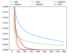
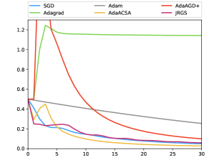
Figure 13: Function value achieved using 2000 iterations and 30 iterations, respectively, for Nesterov’s “worst function”.

	1e-1	1e-2	1e-3	1e-4	1e-5
SGD	16	400	$>$2000	$>$2000	$>$2000
AdaGrad	101	104	$>$2000	$>$2000	$>$2000
Adam	64	149	570	1055	1697
AdaACSA	10	73	275	387	431
AdaAGD+	30	154	525	934	1633
JRGS	18	136	278	495	880

Table 3: Evaluation on Nesterov’s “worst function in the world”. For each method, we display the number of iterations before the first iterate with target error is encountered.

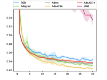
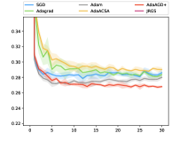
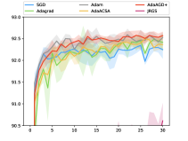
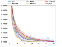
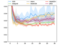
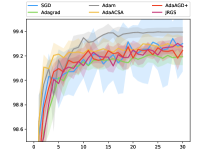
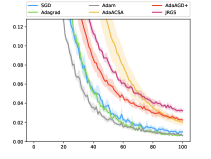
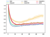
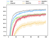
Figure 14: Train losses, test losses, and test accuracies. Top row: logistic regression on MNIST. Middle row: convolutional neural network on MNIST. Bottom row: residual network on CIFAR-10. The plotted lines correspond to values averaged over $5$ runs (except for AdaGrad on CIFAR-10, where one run failed to converge). Shaded areas represent the standard deviation.

logistic	train loss	test loss	test accuracy
SGD	2.44e-1±0.38e-2	2.86e-1±0.46e-2	92.25±0.21
AdaGrad	2.31e-1±0.27e-2	2.84e-1±0.42e-2	92.41±0.20
Adam	2.35e-1±0.17e-2	2.80e-1±0.22e-2	92.53±0.12
AdaACSA	2.23e-1±0.10e-2	2.90e-1±0.28e-2	92.36±0.13
AdaAGD+	2.38e-1±0.15e-2	2.68e-1±0.14e-2	92.57±0.09
JRGS	3.35e-1±1.22e-2	4.42e-1±1.15e-2	90.61±0.40
CNN	train loss	test loss	test accuracy
SGD	10.46e-4±207.62e-5	4.06e-2±1.39e-2	99.30±0.23
AdaGrad	7.32e-4±25.06e-5	2.83e-2±0.17e-2	99.19±0.07
Adam	0.05e-4±0.04e-5	3.28e-2±0.24e-2	99.39±0.04
AdaACSA	0.18e-4±0.71e-5	3.93e-2±0.26e-2	99.28±0.08
AdaAGD+	10.18e-4±57.92e-5	2.49e-2±0.18e-2	99.24±0.04
JRGS	4.43e-4±7.32e-5	3.33e-2±0.44e-2	99.27±0.08
ResNet18	train loss	test loss	test accuracy
SGD	0.10e-1±0.19e-2	0.50±1.11e-2	90.83±0.24
AdaGrad*	0.07e-1±0.05e-2	0.61±2.01e-2	88.50±0.35
Adam	0.06e-1±0.09e-2	0.48±1.15e-2	91.44±0.18
AdaACSA	0.20e-1±0.31e-2	1.00±9.13e-2	83.48±1.15
AdaAGD+	0.23e-1±0.18e-2	0.60±2.79e-2	88.10±0.60
JRGS	0.32e-1±0.16e-2	0.55±3.24e-2	88.20±0.55

Table 4: Comparison between optimization methods for logistic regression on MNIST/convolutional neural network on MNIST/residual network on CIFAR-10.

We empirically validated our adaptive accelerated algorithms, AdaACSA and AdaAGD+, by testing them on a series of standard models encountered in machine learning. While the analyses we provided are specifically crafted for convex objectives, we observed that these methods exhibits good behavior in the non-convex settings corresponding to training deep learning models. This may be motivated by the fact that a significant part of the optimization performed when training such a model occurs within convex regions (Leclerc and Madry, 2020).

Algorithms.

We evaluated our AdaACSA and AdaAGD+ algorithms against three popular methods, SGD with momentum, AdaGrad, and Adam. We also evaluated the algorithms against the recent method of Joulani et al. (2020) which we refer to as JRGS. We performed extensive hyper-parameter tuning, such that each method we compare against has the opportunity to exhibit its best possible performance. We give the complete experimental details in Sections K.1-K.3.

Synthetic experiment.

First, we tested all the methods on a synthetic example, known as Nesterov’s “worst function in the world”, which is a canonical example used for testing accelerated gradient methods (Nesterov, 2013):

$$f(x)=\frac{1}{2}\left(x_{1}^{2}+x_{n}^{2}+\sum_{i=1}^{n-1}\left(x_{i}-x_{i+1}\right)^{2}\right)-x_{1}$$

We see that AdaACSA easily beats all the other methods. In Table 3 we show for each method the number of iterations before finding a solution with a fixed target error in function value. We plot the values of $f$ in Figure 13.

Classification experiments.

Additionally, we tested these optimization methods on three different classification models typically encountered in machine learning. The first one is logistic regression on the MNIST dataset. This is a simple convex objective for which AdaACSA achieves the best training loss, while AdaAGD+ achieves the best test loss. The second is a convolutional neural network on the MNIST dataset. Despite non-convexity, both our methods behave well, and AdaAGD+ achieves the best test loss. The third is a residual network for the CIFAR-10 classification task. We report the training losses, test losses and test accuracies achieved in Table 4. In Figure 14 we plot these values, averaged over $5$ runs.

Discussion.

We verified experimentally that AdaACSA and AdaAGD+ behave very well on convex objectives, as anticipated by theory. For practical non-convex objectives, they show a remarkable degree of robustness, managing to reach close to zero training loss. By contrast, JRGS requires a significant amount of tuning in order to converge – our experiments show that in non-convex settings, without properly constraining the domain to a small $\ell_{\infty}$ ball, it is very hard for it to achieve any nontrivial progress.

K.1 Experimental Setup

We tested each method with its optimal hyper-parameter initialization. More specifically, for each of these methods we first search the hyper-parameter configuration that returns the best training loss after a fixed number of epochs. Then we report experimental results under this choice of hyper-parameters.

For each tested method, we do a grid search over learning rates in $\left\{1,0.5\right\}\times\left\{10^{0},10^{-1},\dots,10^{-4}\right\}$. For SGD we test multiple values for the momentum $\mu=\left\{0.0,0.5,0.9\right\}$. For Adam we we test both the standard algorithm and the AMSGrad version (Reddi et al., 2018).

Notably, AdaAGD+ and JRGS are methods designed specifically for the constrained setting. Indeed, there are simple cases where removing the constraint in the optimization steps may cause them to diverge. We observed that they tend to behave better when adding constraints, even for simple examples. Therefore we run them with a generic $\ell_{\infty}$ radius of $1$, unless otherwise specified. We discuss more about this aspect in Section K.3.

K.1.1 Models and Learning Rates

Here we describe the specific network architectures we used, and the learning rates that achieved the best results after a hyper-parameter search, which we used for our final experiments.

Synthetic Experiment.

We verify experimentally that AdaACSA indeed achieves an accelerated convergence rate for convex objectives. To this end, we test all the methods on Nesterov’s “worst function in the world” Nesterov (2013):

$$f(x)=\frac{1}{2}\left(x_{1}^{2}+x_{n}^{2}+\sum_{i=1}^{n-1}\left(x_{i}-x_{i+1}\right)^{2}\right)-x_{1}\ ,$$ (27)

which is a canonical example that proves tightness of accelerated gradient methods. In our setup we used $n=100$. We ran each method for $2000$ iterations after grid searching for the best hyper-parameter configuration.

We optimized the function from (27). We found the best results using a learning rate of $0.1$ for SGD with $0.9$ momentum, learning rate of $1.0$ for AdaGrad, learning rate of $0.01$ for Adam (with identical behavior whether AMSGrad was used or not), learning rate of $1.0$ for AdaACSA and learning rate of $0.5$ for JRGS. Since AdaGrad and AdaACSA achieved the best convergence with rate $1.0$ we additionally tested them with learning rate $10.0$, but failed to achieve comparable results. With this higher rate, AdaACSA eventually reached the same precision, but required more iterations.

Logistic Regression.

We test these optimization methods on the multi-class logistic regression using the MNIST dataset, which exhibits a simple convex objective. More specifically, our model consists of a single linear layer with cross entropy loss. We train with a minibatch size of 128, as in standard setups.

The model consists of a single linear layer with cross entropy loss. The hyper-parameter search revealed a learning rate of $0.05$ for SGD with $0.5$ momentum, learning rate $0.1$ for AdaGrad, learning rate $0.001$ for Adam with the AMSGrad option activated, learning rate $0.1$ for AdaACSA, and $0.005$ for JRGS.

We ran each optimization method for $30$ epochs with the optimal hyper-parameters setting found via grid search; in each case we ran the method starting from $5$ different random seeds, and reported the mean and standard deviation of train/test losses and test accuracies. The averaged values are reported in Figure 14. The graph for JRGS does not entirely appear in the figure, since the losses it achieves are significantly larger.

Convolutional Neural Network.

We also test the methods on convolutional neural networks (CNN’s). Again, we consider the MNIST classification task. Similarly to the logistic regression experiment, we train with a batch size of $128$ for $30$ epochs.

The model is standard – it contains two stages of 2-d convolutions with a kernel of size $5$, followed by max pooling and ReLU. These are followed by a linear layer, a ReLU layer, and another linear layer, to which we apply cross entropy loss.

We use a learning rate of $0.05$ for SGD with momentum $0.9$, learning rate $0.01$ for AdaGrad, learning rate $0.001$ for Adam with the AMSgrad option activated, learning rate $0.01$ for AdaACSA, and learning rate $0.005$ for JRGS.

This experiment confirms that JRGS is meant to be used only for optimizing convex functions. We notice a drastic difference when switching the architecture from linear to CNN. In the former case the method converges fast, in the latter it fails completely when running it in the same regime as AdaAGD+, with a radius of $1.0$. We reduced the radius to $0.1$ and noticed that all of a sudden the accuracy improved drastically, from as good as random to close to $100$. This suggests that within a small radius the function is locally convex, and hence JRGS exhibits appropriate behavior. However, as opposed to the other methods, which seem to exhibit significant tolerance to non-convexity, this one is extremely fragile. We therefore include results for JRGS with a radius of $0.1$. In Section K.2 we discuss more about this aspect.

Train losses, test losses and test accuracies over $30$ epochs are reported in Figure 14. The values achieved at the end are reported in Table 4.

Residual Network.

We also run tests on the CIFAR-10 dataset, for which we train a standard ResNet18 model (He et al., 2016). We used the ResNet18 model as described in (He et al., 2016), for which we used a standard implementation.

In order to pick hyperparameters, we repeat the experiments previously described and run each setup for $40$ epochs. For JRGS and AdaAGD+, which are better suited for constrained optimization we pick a radius of $2.0$. We made this choice since models we trained with vanilla Adam achieved the best test accuracy with weights that are at most $1.3$ in $\ell_{\infty}$.

For AdaGrad one of the runs failed to converge, so we discarded it, and returned the average of the $4$ remaining runs.

We plot train losses, test losses and test accuracies in Figure 14. While Adam and SGD seem to obtain the best test accuracies, we see that in this regard AdaAGD+, JRGS and AdaGrad are competitive. We note however that AdaGrad exhibits some significant lack of robustness, since for one run it failed to converge, and that JRGS could be run only after some tuning by constraining it to run only within a specific small region around the origin.

We found the best results using a learning rate of $0.1$ for SGD with $0.5$ momentum, learning rate of $0.01$ for Adagrad, learning rate of $0.001$ for Adam with AMSgrad, learning rate of $0.1$ for AdaACSA, learning rate of $0.5$ for AdaAGD+ and and learning rate of $0.01$ for JRGS.

K.2 Failure of JRGS on Nonconvex Domains

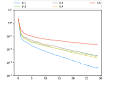
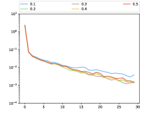
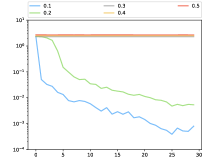
Figure 15: Train losses on a logarithmic scale for AdaACSA, AdaAGD+ and JRGS under different radius constraints. We notice that for non-convex instances (CNN architecture on MNIST) JRGS fails to make any progress unless the optimization domain is sufficiently constrained. By contrast, AdaACSA and AdaAGD+ are fairly robust to non-convexity, as they both empirically exhibit linear convergence even without overconstraining the domain.

Following the discussion from Section K, we show that picking a larger radius makes the JRGS method fail to converge. This stands opposite to the other methods we presented which, although they are designed and analyzed specifically for convex functions, exhibit some degree of robustness to non-convexity. In this experiment we used the learing rates from the CNN experiment in Section K. We run the constrained versions of AdaACSA, AdaAGD+ and JRGS on the MNIST classification task, this time varying the radii of the constrained domain in $\{0.1,0.2,0.3,0.4,0.5\}$. In Figure 15 we see that in the case of JRGS, the performance degrades drastically as radius is increased past $0.2$. On the other hand, the performance of AdaACSA degrades gracefully, as larger radius naturally corresponds to a slower convergence rate. AdaAGD+ is pretty much unaffected by these constraints.

K.3 Discussion on Implementing the Methods

Radius and Learning Rates.

Here we discuss relevant implementation matters. We implemented AdaACSA, AdaAGD+ and JRGS as PyTorch libraries. Compared to the description of the theoretical algorithms, we implemented a series of standard tweaks, to make these more amenable to deploying in the wild.

First, observe that the algorithms we describe do not explicitly include a learning rate. Per the discussion from Section 3, the learning rate corresponds to the radius $R_{\infty}$. However, we allow some further slack by making the learning rate $\eta$ and the radius $R_{\infty}$ two independent parameters. This way we use $\eta$ to adjust the size of the steps we take, and $R_{\infty}$ to define the feasible domain over wich we optimize. This is also a theoretically sound choice, since there is a natural tradeoff between $\eta$ and $R_{\infty}$ which our algorithms optimize by setting these parameters to be equal. In practice, setting them to different values shows some advantage, especially in the case where optimization happens in a much smaller region than the anticipated $\ell_{\infty}$ ball of radius $R_{\infty}$.

Constrained vs Unconstrained Optimization.

Let $D_{0}=I$, $z_{0}=x_{0}$, $\gamma_{0}=1$, $\eta>0$. For $t=0,\dots,T-1$, update: $\displaystyle g_{t}$ $\displaystyle=\widetilde{\nabla}f(x_{t})\ ,$ (get stochastic gradient) $\displaystyle D_{t+1,i}^{2}$ $\displaystyle=D_{t,i}^{2}+\frac{\gamma_{t}^{2}}{\eta^{2}}\left(g_{t}\right)_{i}^{2}\ ,\text{for all }i\in[d].$ $\displaystyle z_{t+1}$ $\displaystyle=z_{t}-\gamma_{t}D_{t+1}^{-1}g_{t}\ ,$ (gradient step) $\displaystyle y_{t+1}$ $\displaystyle=x_{t}-D_{t}^{-1}g_{t}\ ,$ (mirror step) $\displaystyle\gamma_{t+1}$ $\displaystyle=\frac{1}{2}\left(1+\sqrt{1+4\gamma_{t}^{2}}\right)$ $\displaystyle x_{t+1}$ $\displaystyle=\left(1-\gamma_{t+1}^{-1}\right)y_{t+1}+\gamma_{t+1}^{-1}z_{t+1}\ ,$ (linear coupling) Return $y_{T}$.

Figure 16: Unconstrained AdaACSA algorithm.

While the purpose of this paper is to provide algorithms for constrained optimization, in practical instances it may be desirable to not impose explicit constraints on the domain. The reason is that it is possible that during the entire run of the algorithm, the iterates stay within a small region, and hence adding radius constraints only introduce the need for additional tuning. Also, we note that the standard PyTorch implementations of AdaGrad and Adam do not constrain the domain in any way, yet they both achieve good practical performance.

We therefore included in our implementation an unconstrained version of AdaACSA. The algorithm is very similar to the one described in Figures 2 and 9, with a few key differences. First, just as in the AdaGrad and Adam implementations, we do not constrain the domain. Because of this, the movement $z_{t+1}-z_{t}$ which determines the update to the preconditioner $D_{t}$ can be explicitly written as $z_{t+1}-z_{t}=-\gamma_{t}D_{t}^{-1}\nabla f(x_{t})$. We can therefore use this to slightly alter the algorithm and make it more similar to the vanilla unconstrained AdaGrad, in the sense that rather than using the off-by-one scaling (see more about this in Section I) we first update the preconditioner and then perform the step. This does not fundamentally change the analysis — as a matter of fact the only difference is that the speed of convergence will now depend on $R_{\infty}=\max_{t}\left\|x_{t}-x^{*}\right\|_{\infty}$, which is an unknown parameter.

In Figure 16 we describe the unconstrained stochastic algorithm, which turns out to be an adaptive version of the linear coupling method of Allen-Zhu and Orecchia (2017).

We can verify that this algorithm matches the AdaACSA algorithm by moving the preconditioner update before the update in $z$ and $y$. Expanding the iterations from Figure 9 and setting $\alpha_{t}=\gamma_{t}$ we obtain:

$$x_{t} =\left(1-\gamma_{t}^{-1}\right)y_{t}+\gamma_{t}^{-1}z_{t}\ ,$$

$$D_{t+1,i}^{2} =D_{t,i}^{2}\left(1+\frac{\left(z_{t+1,i}-z_{t,i}\right)^{2}}{2R_{\infty}^{2}}\right)=D_{t,i}^{2}+\frac{\gamma_{t}^{2}\left(g_{t}\right)_{i}^{2}}{2R_{\infty}^{2}}\ ,\text{for all }i\in[d].$$

$$z_{t+1} =\arg\min_{u\in\mathcal{K}}\left\{\gamma_{t}\left\langle\widetilde{\nabla}f(x_{t}),u\right\rangle+\frac{1}{2}\left\|u-z_{t}\right\|_{D_{t}}^{2}\right\}=z_{t}-\gamma_{t}D_{t}^{-1}g_{t}\ ,$$

$$y_{t+1} =\left(1-\gamma_{t}^{-1}\right)y_{t}+\gamma_{t}^{-1}z_{t+1}=x_{t}+\gamma_{t}^{-1}\left(z_{t+1}-z_{t}\right)=x_{t}-D_{t}^{-1}\nabla f(x_{t})\ .$$

Since $\gamma_{0}=1$, we also have $x_{0}=z_{0}$, so we can move the update in $x$ after the one for $y$, and hence we derive exactly the algorithm in Figure 16, after setting $\eta=R_{\infty}\sqrt{2}$. Note that we used the specific steps described in Remark 5.5, i.e. we make the inequality $\left(\alpha_{t+1}-1\right)\gamma_{t+1}\leq\alpha_{t}\gamma_{t}$ tight in order to optimize the growth of $\gamma_{t}$.

References

- Allen-Zhu and Orecchia (2017) Zeyuan Allen-Zhu and Lorenzo Orecchia. Linear coupling: An ultimate unification of gradient and mirror descent. In Innovations in Theoretical Computer Science Conference (ITCS), 2017.
- Bach and Levy (2019) Francis Bach and Kfir Y. Levy. A universal algorithm for variational inequalities adaptive to smoothness and noise. In Conference on Learning Theory (COLT), pages 164–194, 2019.
- Bansal and Gupta (2019) Nikhil Bansal and Anupam Gupta. Potential-function proofs for gradient methods. Theory of Computing, 15(4):1–32, 2019.
- Chen et al. (2018) Xiangyi Chen, Sijia Liu, Ruoyu Sun, and Mingyi Hong. On the convergence of a class of adam-type algorithms for non-convex optimization. In International Conference on Learning Representations (ICLR), 2018.
- Cohen et al. (2018) Michael Cohen, Jelena Diakonikolas, and Lorenzo Orecchia. On acceleration with noise-corrupted gradients. In International Conference on Machine Learning (ICML), pages 1018–1027, 2018.
- Cutkosky (2019) Ashok Cutkosky. Anytime online-to-batch, optimism and acceleration. In International Conference on Machine Learning (ICML), pages 1446–1454, 2019.
- Cutkosky (2020) Ashok Cutkosky. Parameter-free, dynamic, and strongly-adaptive online learning. In International Conference on Machine Learning (ICML), 2020.
- Cutkosky and Sarlos (2019) Ashok Cutkosky and Tamas Sarlos. Matrix-free preconditioning in online learning. In International Conference on Machine Learning (ICML), pages 1455–1464, 2019.
- Défossez et al. (2020) Alexandre Défossez, Léon Bottou, Francis Bach, and Nicolas Usunier. On the convergence of adam and adagrad. arXiv preprint arXiv:2003.02395, 2020.
- Diakonikolas and Orecchia (2018) Jelena Diakonikolas and Lorenzo Orecchia. Accelerated extra-gradient descent: A novel accelerated first-order method. In Innovations in Theoretical Computer Science Conference (ITCS), volume 94, pages 23:1–23:19, 2018.
- Dozat (2016) Timothy Dozat. Incorporating nesterov momentum into adam. In International Conference on Learning Representations (ICLR) Workshop, 2016.
- Duchi et al. (2011) John Duchi, Elad Hazan, and Yoram Singer. Adaptive subgradient methods for online learning and stochastic optimization. Journal of machine learning research, 12(7), 2011.
- Gupta et al. (2018) Vineet Gupta, Tomer Koren, and Yoram Singer. Shampoo: Preconditioned stochastic tensor optimization. In International Conference on Machine Learning (ICML), pages 1842–1850, 2018.
- He et al. (2016) Kaiming He, Xiangyu Zhang, Shaoqing Ren, and Jian Sun. Deep residual learning for image recognition. In Computer Vision and Pattern Recognition (CVPR), pages 770–778, 2016.
- Joulani et al. (2020) Pooria Joulani, Anant Raj, András György, and Csaba Szepesvári. A simpler approach to accelerated stochastic optimization: Iterative averaging meets optimism. In International Conference on Machine Learning (ICML), 2020.
- Kavis et al. (2019) Ali Kavis, Kfir Y. Levy, Francis Bach, and Volkan Cevher. Unixgrad: A universal, adaptive algorithm with optimal guarantees for constrained optimization. In Neural Information Processing Systems (NeurIPS), pages 6257–6266, 2019.
- Kingma and Ba (2014) Diederik P Kingma and Jimmy Ba. Adam: A method for stochastic optimization. arXiv preprint arXiv:1412.6980, 2014.
- Lan (2012) Guanghui Lan. An optimal method for stochastic composite optimization. Mathematical Programming, 133(1-2):365–397, 2012.
- Leclerc and Madry (2020) Guillaume Leclerc and Aleksander Madry. The two regimes of deep network training. arXiv preprint arXiv:2002.10376, 2020.
- Levy (2017) Kfir Levy. Online to offline conversions, universality and adaptive minibatch sizes. In Neural Information Processing Systems (NeurIPS), pages 1613–1622, 2017.
- Levy et al. (2018a) Kfir Y Levy, Alp Yurtsever, and Volkan Cevher. Online adaptive methods, universality and acceleration. In Neural Information Processing Systems (NeurIPS), pages 6500–6509, 2018a.
- Levy et al. (2018b) Kfir Yehuda Levy, Alp Yurtsever, and Volkan Cevher. Online adaptive methods, universality and acceleration. In Neural Information Processing Systems (NeurIPS), pages 6501–6510, 2018b.
- Li and Orabona (2019) Xiaoyu Li and Francesco Orabona. On the convergence of stochastic gradient descent with adaptive stepsizes. In Artificial Intelligence and Statistics (AISTATS), pages 983–992, 2019.
- McMahan and Streeter (2010) H. Brendan McMahan and Matthew J. Streeter. Adaptive bound optimization for online convex optimization. In Conference on Learning Theory (COLT), pages 244–256, 2010.
- Mohri and Yang (2016) Mehryar Mohri and Scott Yang. Accelerating online convex optimization via adaptive prediction. In Artificial Intelligence and Statistics (AISTATS), pages 848–856, 2016.
- Nemirovski (2004) Arkadi Nemirovski. Prox-method with rate of convergence o (1/t) for variational inequalities with lipschitz continuous monotone operators and smooth convex-concave saddle point problems. SIAM Journal on Optimization, 15(1):229–251, 2004.
- Nesterov (2015) Yu Nesterov. Universal gradient methods for convex optimization problems. Mathematical Programming, 152(1-2):381–404, 2015.
- Nesterov (1998) Yurii Nesterov. Introductory lectures on convex programming volume i: Basic course. Lecture notes, 3(4):5, 1998.
- Nesterov (2013) Yurii Nesterov. Introductory lectures on convex optimization: A basic course, volume 87. Springer Science & Business Media, 2013.
- Reddi et al. (2018) Sashank J Reddi, Satyen Kale, and Sanjiv Kumar. On the convergence of adam and beyond. In International Conference on Learning Representations (ICLR), 2018.
- Tieleman and Hinton (2012) Tijmen Tieleman and Geoffrey Hinton. Lecture 6.5-rmsprop: Divide the gradient by a running average of its recent magnitude. COURSERA: Neural networks for machine learning, 4(2):26–31, 2012.
- Ward et al. (2019) Rachel Ward, Xiaoxia Wu, and Leon Bottou. Adagrad stepsizes: sharp convergence over nonconvex landscapes. In International Conference on Machine Learning (ICML), pages 6677–6686, 2019.
- Zou et al. (2018) Fangyu Zou, Li Shen, Zequn Jie, Ju Sun, and Wei Liu. Weighted adagrad with unified momentum. arXiv preprint arXiv:1808.03408, 2018.
- Zou et al. (2019) Fangyu Zou, Li Shen, Zequn Jie, Weizhong Zhang, and Wei Liu. A sufficient condition for convergences of adam and rmsprop. In Computer Vision and Pattern Recognition (CVPR), pages 11127–11135, 2019.