Kinetic functions for nonclassical shocks,
entropy stability, and discrete summation by parts

Abstract

We study nonlinear hyperbolic conservation laws with non-convex flux in one space dimension and, for a broad class of numerical methods based on summation by parts operators, we compute numerically the kinetic functions associated with each scheme. As established by LeFloch and collaborators, kinetic functions (for continuous or discrete models) uniquely characterize the macro-scale dynamics of small-scale dependent, undercompressive, nonclassical shock waves. We show here that various entropy-dissipative numerical schemes can yield nonclassical solutions containing classical shocks, including Fourier methods with (super-) spectral viscosity, finite difference schemes with artificial dissipation, discontinuous Galerkin schemes with or without modal filtering, and TeCNO schemes. We demonstrate numerically that entropy stability does not imply uniqueness of the limiting numerical solutions for scalar conservation laws in one space dimension, and we compute the associated kinetic functions in order to distinguish between these schemes. In addition, we design entropy-dissipative schemes for the Keyfitz-Kranzer system whose solutions are measures with delta shocks. This system illustrates the fact that entropy stability does not imply boundedness under grid refinement.

1 Introduction

1.1 Objective and background

We present and analyze here several classes of entropy-stable and semi-discrete schemes for nonlinear hyperbolic problems, next investigate numerically the behavior of weak solutions, and demonstrate certain important features or limitations of these schemes. In particular, we observe that entropy-stable schemes can converge to different weak solutions. Hence, we are interested in qualitative properties of weak solutions $u=u(t,x)$ to nonlinear hyperbolic conservation laws

$$\partial_{t}u+\partial_{x}f(u)=0,\qquad u|_{t=0}=u_{0},$$ (1)

posed on a bounded domain $\Omega\subset\mathbb{R}$ (subjected to suitable boundary conditions). Here, $u_{0}$ is a prescribed initial data defined on $\Omega$, while the flux $f=f(u)$ is a prescribed nonlinear function of the unknown $u$. In general, weak solutions to (1) (understood in the sense of distributions) contain shock waves, and a central issue in the theory of nonlinear hyperbolic equations is formulating suitable admissibility criteria for the selection of shocks. For scalar conservation laws with convex flux (such as Burgers’ equation) a single entropy inequality

$$\partial_{t}U(u)+\partial_{x}F(u)\leq 0,$$ (2)

associated with a strictly convex entropy pair $(U,F)$, suffices to single out a unique weak solution [10, 55] to the initial value problem (1).

However, this is not true for conservation laws with non-convex flux [55, Remark 2], for instance for the cubic conservation law $\partial_{t}u+\partial_{x}u^{3}=0$ [39, Chapter II]. While it is well-known that weak solutions to conservation laws can be generated as vanishing viscosity limits, that is, as limits (when $\varepsilon\to 0$) of solutions to

$$\partial_{t}u+\partial_{x}f(u)=\varepsilon\partial_{x}^{2}u,$$ (3)

other regularization operators are equally relevant in physical applications and generate weak solutions that may not satisfy the standard selection criteria. In fact, the single entropy inequality (2) permits also nonclassical shocks of undercompressive type, which in turn should be characterized via the notion of a kinetic function; for an overview of the theory, see LeFloch [38, 39, 40]. The role of small-scale effects in weak solutions (for instance when capillarity effect is included) and the numerical approximation of nonclassical solutions were extensively investigated in the past two decades; see the pioneering papers [27, 22, 23], as well as the advances in [43, 5, 1] and the references therein. More recently, the class of well-controlled dissipation (WCD) schemes which capture diffusive-dispersive shocks at any arbitrary order of accuracy, was proposed in [42, 45, 46].

1.2 Main contributions in this paper

We proceed here by presenting first a broad class of numerical methods which are based on summation-by-parts (SBP) operators and, importantly, are entropy-satisfying in the sense that they satisfy a discrete form of the entropy inequality. Recall that entropy-conservative schemes were constructed in a pioneering work by Tadmor [77, 75] (second-order accuracy) and LeFloch and Rohde [44] (third-order accuracy), and later extended in [41] (high-order accuracy in a periodic domain) and [13, 56, 6] (bounded domain and non-uniform grids). The entropy inequality is essential since it ensures a fundamental $L^{2}$ nonlinear stability property, but does not guarantee convergence to classical entropy solutions. The entropy-satisfying numerical methods developed and analyzed in the present paper are based on the notion of SBP operators in [36], which recently have gained a lot of interest. Nowadays, many classes of numerical methods can be formulated within a unifying SBP framework, including finite difference [72], finite volume [53], finite element [19, 25], and flux reconstruction schemes [68]. Importantly, these semi-discretizations can be made entropy-satisfying and the main stability estimates can also be transferred to fully discrete numerical methods by applying a relaxation approach [30, 69, 65, 64, 61, 66, 51].

It is precisely our purpose here to demonstrate that a broad class of entropy-satisfying schemes generate nonclassical shocks and, in addition, to compute the associated kinetic functions. We focus on the spatial part and apply sufficiently accurate time integration schemes in order to eliminate any significant errors from that part. We restrict convergence studies of the numerical methods to numerical experiments and grid refinement studies. In particular, we observe convergence of numerical solutions of nonlinear scalar conservation laws in one space dimension, in contrast to the behavior of nonlinear systems in multiple space dimensions [18, 15]. However, even when the numerical methods satisfy a single entropy inequality, the numerically converged solutions can still approximate nonclassical shocks.

1.3 Outline of this paper

In Section 2, entropy-stable discretizations based on SBP operators are recalled and discussed. Next, in Sections 3 and 4, we revisit the uniqueness issue for nonlinear conservation laws and, in Section 5, for a variety of schemes we numerically compute the corresponding kinetic function associated with the cubic conservation law. This study is then extended to a quartic conservation law in Section 6. Finally, in Section 7 we turn our attention toward the Keyfitz-Kranzer system, for which we develop and apply a broad class of entropy-stable schemes.

2 Summation-by-parts operators and entropy stability

2.1 Notation

In this section, some general notions about SBP operators are reviewed and a notation to be used throughout the following sections is introduced. For more information on SBP operators, we refer to the review articles [73, 12] and references cited therein. We consider the nonlinear hyperbolic system of conservation laws

$$\partial_{t}u(t,x)+\partial_{x}f\bigl{(}u(t,x)\bigr{)} =0, t\in(0,T),\,x\in\Omega,$$ (4)

$$u(0,x) =u_{0}(x), x\in\Omega,$$

posed on the spatial domain $\Omega\subseteq\mathbb{R}$ in one space dimension, supplemented with appropriate boundary data or periodic boundary conditions. Here, $u\colon(0,T)\times\Omega\to\Upsilon\subseteq\mathbb{R}^{m}$ are the conserved variables and $f\colon\Upsilon\to\mathbb{R}^{m}$ is referred to as the flux. Using the method of lines, a semi-discretization is introduced at first and a suitable time integration scheme is applied to the resulting set of ordinary differential equations, e.g. a Runge-Kutta method. For the semi-discretization, the spatial domain $\Omega\subseteq\mathbb{R}$ is divided into non-overlapping elements $\Omega_{l}$, i.e. we have $\bigcup_{l}\Omega_{l}=\Omega$ and $\mathring{\Omega}_{l}\cap\mathring{\Omega}_{k}=\varnothing$ if $l\neq k$, where $\mathring{\Omega}_{l}$ is the interior of the element $\Omega_{l}$. In each element the numerical solution is represented by its values $\underline{u}=(\underline{u}_{1},\dots,\underline{u}_{K})^{T}$ on a grid with nodes $x_{1},\dots,x_{K}$, i.e. we write $\underline{u}_{i}=u(x_{i})$. All nonlinear operations of interest are then defined pointwise, for instance $\underline{f}_{i}=f(\underline{u}_{i})$. The discrete derivative will be represented by a matrix $\underline{\underline{D}}\,\in\mathbb{R}^{K\times K}$, referred to as the derivative matrix, and the discrete scalar product approximating the standard $L^{2}$ scalar product will be represented by a symmetric and positive definite matrix, denoted by $\underline{\underline{M}}\,\in\mathbb{R}^{K\times K}$ (mass/norm matrix). In the following, the notation in [68, 67] is used. A table with translation rules to other common notations for finite difference and spectral element methods can be found in [58].

2.2 Periodic setting

Consider the domain $\Omega=({x_{L}},{x_{R}})$ and absolutely continuous functions $u,v\colon\mathbb{R}\to\mathbb{R}$ that are periodic with period $\mathinner{\!\left\lvert\Omega\right\rvert}={x_{R}}-{x_{L}}$. Then, integration by parts gives

$$\int_{x_{L}}^{x_{R}}u\,(\partial_{x}v)=\big{[}uv\big{]}_{x_{L}}^{x_{R}}-\int_{x_{L}}^{x_{R}}(\partial_{x}u)\,v,$$ (5)

where the boundary term vanishes due to periodicity. This is mimicked at the discrete level by writing $\underline{u}^{T}\underline{\underline{M}}\,\underline{\underline{D}}\,\underline{v}=-\underline{u}^{T}\underline{\underline{D}}{{}^{T}}\underline{\underline{M}}\,\underline{v}.$ Requiring that this relation holds for all $\underline{u},\underline{v}\in\mathbb{R}^{K}$ results in the following definition. With some abuse of notation, the derivative matrix $\underline{\underline{D}}\,$ will also be called SBP (derivative) operator if the corresponding mass/norm matrix can be deduced from the context.

Definition 2.1.

A periodic SBP operator (or summation-by-parts operator) consists of a derivative matrix $\underline{\underline{D}}\,$ and a symmetric and positive definite mass/norm matrix $\underline{\underline{M}}\,$ such that $\underline{\underline{M}}\,\underline{\underline{D}}\,+\underline{\underline{D}}{{}^{T}}\underline{\underline{M}}\,=\underline{\underline{0}}\,.$

Example 2.2.

Periodic central finite difference approximations of the first derivative yield SBP operators with mass matrix $\underline{\underline{M}}\,=\Delta x\underline{\underline{\operatorname{I}}}\,$, where $\underline{\underline{\operatorname{I}}}\,$ is the identity matrix and $\Delta x$ the grid spacing. In other words, periodic central finite difference approximations of the first derivative result in skew-symmetric derivative matrices $\underline{\underline{D}}\,$.

Example 2.3.

Fourier (pseudo-) spectral methods computing the derivative via the discrete Fourier transform (via FFT) also yield SBP operators with a multiple of the identity matrix as mass matrix.

2.3 Non-periodic setting

Consider again the domain $\Omega=({x_{L}},{x_{R}})$ and absolutely continuous functions $u,v\colon\mathbb{R}\to\mathbb{R}$. Without requiring periodicity, integration by parts gives

$$\int_{x_{L}}^{x_{R}}u\,(\partial_{x}v)+\int_{x_{L}}^{x_{R}}(\partial_{x}u)\,v=\big{[}uv\big{]}_{x_{L}}^{x_{R}}.$$ (6)

Similarly to the periodic case, this is mimicked at the discrete level by

$$\underline{u}^{T}\underline{\underline{M}}\,\underline{\underline{D}}\,\underline{v}+\underline{u}^{T}\underline{\underline{D}}{{}^{T}}\underline{\underline{M}}\,\underline{v}=\underline{u}^{T}\underline{\underline{R}}{{}^{T}}\underline{\underline{B}}\,\underline{\underline{R}}\,\underline{v},$$ (7)

where a restriction matrix $\underline{\underline{R}}\,$ performing an interpolation to the boundary nodes ${x_{L}},{x_{R}}$ and a boundary matrix $\underline{\underline{B}}\,=\operatorname{diag}\left(-1,1\right)$ have been introduced. Requiring that the relation above holds for all $\underline{u},\underline{v}\in\mathbb{R}^{K}$ results in the following definition.

Definition 2.4.

A (non-periodic) SBP operator (i.e. summation-by-parts operator) consists of a derivative matrix $\underline{\underline{D}}\,$, a symmetric and positive definite mass/norm matrix $\underline{\underline{M}}\,$, a restriction matrix $\underline{\underline{R}}\,$, and the boundary matrix $\underline{\underline{B}}\,=\operatorname{diag}\left(-1,1\right)$ such that $\underline{\underline{M}}\,\underline{\underline{D}}\,+\underline{\underline{D}}{{}^{T}}\underline{\underline{M}}\,=\underline{\underline{R}}{{}^{T}}\underline{\underline{B}}\,\underline{\underline{R}}\,.$ The order of accuracy of the approximation $\underline{u}^{T}\underline{\underline{R}}{{}^{T}}\underline{\underline{B}}\,\underline{\underline{R}}\,\underline{v}\approx[uv]_{x_{L}}^{x_{R}}$ should be at least the order of accuracy of the derivative matrix $\underline{\underline{D}}\,$.

SBP operators can be used both in single element discretizations and in multiple element discretizations where the domain $\Omega$ is divided into smaller elements as described at the beginning of this section. In the latter case, SBP operators are used on each element. Typically, the operators are developed on a reference element and a coordinate transformation is used to map all quantities between the physical and the reference element. If not stated otherwise, affine-linear coordinate mappings will be used in the following.

Example 2.5.

1. Classical finite difference SBP operators have been proposed by many researchers and many examples can be found in the review articles [73, 12] and references cited therein.

2. Polynomial collocation methods based on Legendre polynomials of degree $p=K-1$ yield SBP operators if the derivative matrix $\underline{\underline{D}}\,$ and the restriction matrix $\underline{\underline{R}}\,$ are exact for polynomials of degree $\leq p$ and the mass matrix $\underline{\underline{M}}\,$ is chosen such that it is exact for polynomials of degree $\leq p-1$, since all integrals in (7) can be evaluated exactly in this case, cf. [35]. In particular, polynomial collocation methods based on the Gauss, Radau, or Lobatto Legendre nodes yield SBP operators, see also [19, 11, 26].

2.4 Boundary procedures

If periodic SBP operators are used (for periodic problems), no boundary conditions have to be enforced. If non-periodic boundaries or multiple elements are considered, exterior (at the boundary of the domain $\Omega$) or interior (between two elements) boundary conditions have to be enforced. Here, the prescription of boundary conditions via simultaneous approximation terms using numerical fluxes as in finite volume methods will be used.

Definition 2.6.

A numerical flux is a Lipschitz continuous mapping $f^{\mathrm{num}}\colon\Upsilon^{2}\to\mathbb{R}^{m}$ that is consistent with the flux $f$ of the conservation law (4), i.e. $\text{ for all }u\in\Upsilon\colon f^{\mathrm{num}}(u,u)=f(u)$.

A semi-discretization of the conservation law $\partial_{t}u+\partial_{x}f(u)=0$ on an element will usually be of the form

$$\partial_{t}\underline{u}+\underline{\mathrm{VOL}}=\underline{\mathrm{SAT}},$$ (8)

where $\underline{\mathrm{VOL}}$ are volume terms approximating the divergence $\partial_{x}f(u)$ in the interior and $\underline{\mathrm{SAT}}$ is a simultaneous approximation term [3, 4] enforcing boundary conditions in a suitably weak sense. Typical forms might be

$$\underline{\mathrm{VOL}}=\underline{\underline{D}}\,\underline{f},\qquad\underline{\mathrm{SAT}}=-\underline{\underline{M}}{{}^{-1}}\underline{\underline{R}}{{}^{T}}\underline{\underline{B}}\,\left(\underline{f}^{\mathrm{num}}-\underline{\underline{R}}\,\underline{f}\right),$$ (9)

where $\underline{\underline{R}}\,\underline{f}=(f_{L},f_{R})^{T}$ is the interpolation of the flux $\underline{f}$ to the boundary and $\underline{f}^{\mathrm{num}}=(f^{\mathrm{num}}_{L},f^{\mathrm{num}}_{R})^{T}$ is the numerical flux at the boundaries. At a given boundary between the elements $l$ and $l+1$, two values of the numerical solution are given via interpolation: The value $u_{-}=u^{(l)}_{R}$ of the numerical solution at the right-hand side of cell $l$ and the value $u_{+}=u^{(l+1)}_{L}$ of the numerical solution at the left-hand side of cell $l+1$. Then, the unique numerical flux between the elements $l$ and $l+1$ is computed as $f^{\mathrm{num}}(u_{-},u_{+})$; see the illustration in Figure 1.

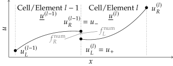
Figure 1: Visualization of the notation used for multiple element discretizations using SATs with numerical fluxes. The numerical flux at the boundary between the elements $l-1$ and $l$ is computed as $f^{\mathrm{num}}(u_{-},u_{+})$, where $u_{-}$ ($u_{+}$) is the value of the numerical solution to the left (right) of the interface. In element $l-1$ ($l$), this numerical flux is at the right (left) hand side of the element and called $f^{\mathrm{num}}_{R}$ ($f^{\mathrm{num}}_{L}$).

2.5 Entropy stability

Throughout, we assume that our system of conservation laws (4) is equipped with an entropy function. Recall that a convex function $U\colon\Upsilon\to\mathbb{R}$ is an entropy for the conservation law (4), if there is an entropy flux $F\colon\Upsilon\to\mathbb{R}$ fulfilling $\partial_{u}U(u)\cdot\partial_{u}f(u)=\partial_{u}F(u)$. The entropy variables are $w(u)=U^{\prime}(u)$ and the flux potential is $\psi=w\cdot f-F$. Thus, if $U$ is an entropy and $u$ a smooth solution of the conservation law (4), the entropy generates the conservation law $\partial_{t}U(u)+\partial_{x}F(u)=0$. As an admissibility criterion, the entropy inequality

$$\partial_{t}U(u)+\partial_{x}F(u)\leq 0.$$ (10)

is imposed for weak solutions. The flux potential $\psi$ is the potential of the flux $f$ with respect to the entropy variables $w$, i.e. $\partial_{w}\psi(w)=f(w)$, where $f(w)$ should be read as $f\bigl{(}u(w)\bigr{)}$.

Example 2.7.

For scalar conservation laws, the $L^{2}$ entropy $U(u)=\frac{1}{2}u^{2}$ can be used. It is strictly convex and the entropy variables are $w(u)=U^{\prime}(u)=u$. The flux potential is given by $\psi(u)=\int^{u}f(v)\operatorname{d\!}v$.

Building on the seminal work of Tadmor [77, 75] on second-order schemes, extended to arbitrary order of accuracy in [44], semi-discrete entropy-stable schemes can be constructed as entropy-conservative schemes and additional dissipation mechanisms. The basic ingredient are entropy conservative two-point numerical fluxes used in finite volume methods.

Definition 2.8.

A numerical flux is entropy-conservative (EC) for an entropy $U$ with entropy variables $w$ and flux potential $\psi$, if

$$\text{ for all }u_{-},u_{+}\in\Upsilon\colon\quad\bigl{(}w(u_{+})-w(u_{-})\bigr{)}\cdot f^{\mathrm{num}}(u_{-},u_{+})=\psi(u_{+})-\psi(u_{-}).$$ (11)

The numerical flux is entropy-stable (ES), if

$$\text{ for all }u_{-},u_{+}\in\Upsilon\colon\quad\bigl{(}w(u_{+})-w(u_{-})\bigr{)}\cdot f^{\mathrm{num}}(u_{-},u_{+})\leq\psi(u_{+})-\psi(u_{-}).$$ (12)

Using the jump operator $\raisebox{-2.5pt}{\leavevmode\resizebox{0.0pt}{7.5pt}{\raisebox{2.5pt}{$[\mkern-3.0mu[$}}}a\raisebox{-2.5pt}{\leavevmode\resizebox{0.0pt}{7.5pt}{\raisebox{2.5pt}{$]\mkern-3.0mu]$}}}\mathrel{\mathop{\ordinarycolon}}=a_{+}-a_{-}$ and the notation $a_{\pm}=a(u_{\pm})$, these equations can be written as $\raisebox{-2.5pt}{\leavevmode\resizebox{0.0pt}{7.5pt}{\raisebox{2.5pt}{$[\mkern-3.0mu[$}}}w\raisebox{-2.5pt}{\leavevmode\resizebox{0.0pt}{7.5pt}{\raisebox{2.5pt}{$]\mkern-3.0mu]$}}}\cdot f^{\mathrm{num}}=\raisebox{-2.5pt}{\leavevmode\resizebox{0.0pt}{8.3333pt}{\raisebox{2.5pt}{$[\mkern-3.0mu[$}}}\psi\raisebox{-2.5pt}{\leavevmode\resizebox{0.0pt}{8.3333pt}{\raisebox{2.5pt}{$]\mkern-3.0mu]$}}}$ and $\raisebox{-2.5pt}{\leavevmode\resizebox{0.0pt}{7.5pt}{\raisebox{2.5pt}{$[\mkern-3.0mu[$}}}w\raisebox{-2.5pt}{\leavevmode\resizebox{0.0pt}{7.5pt}{\raisebox{2.5pt}{$]\mkern-3.0mu]$}}}\cdot f^{\mathrm{num}}\leq\raisebox{-2.5pt}{\leavevmode\resizebox{0.0pt}{8.3333pt}{\raisebox{2.5pt}{$[\mkern-3.0mu[$}}}\psi\raisebox{-2.5pt}{\leavevmode\resizebox{0.0pt}{8.3333pt}{\raisebox{2.5pt}{$]\mkern-3.0mu]$}}}$, respectively.

Remark 2.9.

Entropy stability of a numerical method does not imply general stability of the scheme, since further robustness properties might be necessary to guarantee that the numerical solution does not blow up. Moreover, for linear equations, (strong) stability is the discrete analogue of (strong) well-posedness of the continuous problem, cf. [73, 52]. This is in general not the case for nonlinear equations. Thus, it might be better to speak about entropy-conservative and entropy-dissipative schemes. Nevertheless, since it is more common in the literature to speak about entropy-stable schemes, this term will be used here.

Entropy-conservative numerical fluxes can be used to construct high-order entropy conservative semi-discretizations using SBP operators via the volume terms

$$\underline{\mathrm{VOL}}_{i}=\sum_{k=1}^{K}{\underline{\underline{D}}\,}_{i,k}2f^{\mathrm{vol}}(\underline{u}_{i},\underline{u}_{k}),$$ (13)

where $f^{\mathrm{vol}}$ is an entropy-conservative numerical flux called volume flux (since it it used for the volume terms) and $\underline{u}_{i},\underline{u}_{k}$ are the values of the discrete solution at the grid nodes. The following result can be found in [56, 6] and is a generalisation of [13, Theorem 3.1].

Theorem 2.10.

If the volume flux $f^{\mathrm{vol}}$ is smooth and symmetric, the flux differencing form (13) is an approximation of the same order of accuracy as the derivative matrices $\underline{\underline{D}}\,$. Here, the derivative matrix does not need to be given by SBP operators.

If the corresponding mass matrix $\underline{\underline{M}}\,$ of an SBP derivative $\underline{\underline{D}}\,$ is diagonal, the volume terms (13) can be written in a locally conservative form. Moreover, if the volume flux is entropy-conservative and the boundary nodes are included, high-order entropy-stable semi-discretizations can be constructed, cf. [13, 56, 6].

Theorem 2.11.

Consider the semi-discretization $\partial_{t}\underline{u}+\underline{\mathrm{VOL}}=\underline{\mathrm{SAT}}$ with volume terms given by (13) and the surface terms

$$\underline{\mathrm{SAT}}=-\underline{\underline{M}}{{}^{-1}}\underline{\underline{R}}{{}^{T}}\underline{\underline{B}}\,\left(\underline{f}^{\mathrm{num}}-\underline{\underline{R}}\,\underline{f}\right).$$ (14)

If the numerical volume flux $f^{\mathrm{vol}}$ is consistent with $f$, symmetric, and entropy-conservative, and both the mass matrix $\underline{\underline{M}}\,$ and the boundary operator $\underline{\underline{R}}{{}^{T}}\underline{\underline{B}}\,\underline{\underline{R}}\,$ are diagonal, the semi-discretization is entropy-conservative/stable across elements, if the numerical surface flux $f^{\mathrm{num}}$ is entropy-conservative/stable. Moreover, there is a locally conservative form for the semi-discrete entropy equation.

Remark 2.12.

Requiring that $\underline{\underline{R}}{{}^{T}}\underline{\underline{B}}\,\underline{\underline{R}}\,$ be diagonal seems to be necessary for general conservation laws. Basically, it states that the boundary nodes have to be included in the computational grid. For some conservation laws, the surface terms (14) can be adapted to allow general SBP operators not including the boundary nodes, e.g. polynomial collocation methods on Gauss-Legendre nodes, cf. [68, 60, 58, 54, 57].

2.6 Dissipation operators

A semi-discretization $\partial_{t}\underline{u}+\underline{\mathrm{VOL}}=\underline{\mathrm{SAT}}$ can be enhanced by artificial dissipation terms $\underline{\mathrm{DISS}}$, resulting in

$$\partial_{t}\underline{u}+\underline{\mathrm{VOL}}=\underline{\mathrm{SAT}}+\underline{\mathrm{DISS}}.$$ (15)

Since entropy stability is investigated by multiplying the semi-discretization by $\underline{w}^{T}\underline{\underline{M}}\,$, the dissipation term $\underline{\mathrm{DISS}}$ should fulfil $\underline{w}^{T}\underline{\underline{M}}\,\underline{\mathrm{DISS}}\leq 0$. Moreover, in order not to influence conservation across elements, the dissipation term should satisfy $\underline{1}^{T}\underline{\underline{M}}\,\underline{\mathrm{DISS}}=\underline{0}$, where $\underline{1}$ is a vector with entries $1$, i.e. the discrete version of the function $x\mapsto 1$.

Example 2.13.

Considering the $L^{2}$ entropy $U(u)=\frac{1}{2}u^{2}$ as in Example 2.7, dissipation operators can be constructed as $\underline{\mathrm{DISS}}=-\underline{\underline{M}}{{}^{-1}}\underline{\underline{S}}\,$, where $\underline{\underline{S}}\,$ is (symmetric and) positive semidefinite and satisfies $\underline{1}^{T}\underline{\underline{S}}\,=\underline{0}$. Such dissipation operators approximating weighted derivatives of even degree have been proposed in [50].

Example 2.14.

For collocation schemes using Legendre polynomials, suitable discretizations of the Legendre derivative operator $u\mapsto\partial_{x}(a\partial_{x}u)$ with $a(x)=1-x^{2}$ can be used. The Legendre polynomials $\varphi_{n}$ are eigenvectors of this operator with eigenvalues $\lambda_{n}=-n(n+1)$. An investigation using this kind of dissipation and SBP operators can be found inter alia in [63].

Example 2.15.

The (super-) spectral viscosity operators investigated in [48, 74, 71, 47, 76, 21, 78] are suitable dissipation operators for the $L^{2}$ entropy $U(u)=\frac{1}{2}u^{2}$, cf. Example 2.7.

Example 2.16.

The so-called TeCNO schemes presented in [16, 14] are designed for periodic boundary conditions. The volume terms are exactly the entropy-conservative ones (13). The dissipation operators are constructed using the ENO procedure and are based on a recent stability result of this reconstruction [17].

2.7 Filtering

Another possibility introducing dissipation is given by filtering. Here, the baseline scheme is used to compute one time step (or only one stage of a Runge-Kutta method) and a dissipative filter is applied afterwards, reducing the total amount of entropy without modifying the total mass. Classical modal filters can also be motivated by the application of a splitting procedure to a semi-discretization enhanced with artificial dissipation. If this dissipation corresponds to a modal basis such as a Legendre basis, the action of the dissipation operator can be realized as modal filtering. Splitting a complete time step into a step using the baseline scheme and an exact integration of the dissipation operator results in this modal filtering approach. However, other filter functions can be used as well.

Example 2.17.

Applying an exponential filter of the form $\exp(-\varepsilon\,\Delta t\,n(n+1))$ corresponds to the exact solution of the equation $\partial_{t}u(t,x)=\partial_{x}\bigl{(}(1-x^{2})\partial_{x}u(t,x)\bigr{)},$ as in Example 2.14. Similar to the super-spectral viscosity approach, the Legendre dissipation operator can be applied $s$ times, resulting in the filter function $\exp(-\varepsilon\,\Delta t\,(n(n+1))^{s})$. Results for modal filters can be found in [79, 24, 63].

3 Revisiting the uniqueness issue for conservation laws

3.1 Periodic boundary conditions

In the following numerical experiments, the fourth-order, ten stage, strong stability preserving explicit Runge-Kutta method SSPRK(10,4) of [29] will be used to advance the numerical solutions up to the final time $T=1$. We treat the cubic conservation law

$$\partial_{t}u(t,x)+\partial_{x}u(t,x)^{3} =0,\quad t\in(0,T),\,x\in({x_{L}},{x_{R}}),$$ (16)

$$u(0,x) =u_{0}(x),\quad x\in({x_{L}},{x_{R}}),$$

supplemented with periodic or other appropriate boundary conditions as described in the following. The initial condition is chosen as $u_{0}(x)=-\sin(\pi x)$ in the domain $({x_{L}},{x_{R}})=(-1,1)$. Using periodic boundary conditions and the $L^{2}$ entropy $U(u)=\frac{1}{2}u^{2}$, the total entropy $\int U$ is conserved for smooth solutions and bounded from above by its initial value for entropy weak solutions. Using the unique entropy-conservative flux (cf. Definition 2.8)

$$f^{\mathrm{vol}}(u_{-},u_{+})=\frac{1}{4}\frac{u_{+}^{4}-u_{-}^{4}}{u_{+}-u_{-}}=\frac{1}{4}\left(u_{+}^{3}+u_{+}^{2}u_{-}+u_{+}u_{-}^{2}+u_{-}^{3}\right)$$ (17)

in the flux difference discretization described in Theorem 2.11 results in the volume terms

$$\underline{\mathrm{VOL}}=\frac{1}{2}\underline{\underline{D}}\,\underline{\underline{u}}\,^{2}\underline{u}+\frac{1}{2}\underline{\underline{u}}\,\underline{\underline{D}}\,\underline{\underline{u}}\,\underline{u}+\frac{1}{2}\underline{\underline{u}}\,^{2}\underline{\underline{D}}\,\underline{u},$$ (18)

where $\underline{\underline{u}}\,=\operatorname{diag}\left(\underline{u}\right)$ are diagonal multiplication operators, performing pointwise multiplication with the values of $\underline{u}$ at the nodes of the grid. These volume terms can be interpreted as approximations to the split form $\frac{1}{2}\bigl{(}\partial_{x}u^{3}+u\partial_{x}u^{2}+u^{2}\partial_{x}u\bigr{)}$. Traditionally, one could also use the following unsplit form, without obtaining an entropy estimate,

$$\underline{\mathrm{VOL}}=\underline{\underline{D}}\,\underline{\underline{u}}{{}^{2}}\underline{u}.$$ (19)

The following semi-discretizations will be used for periodic boundary conditions. For these schemes, the time step is chosen as $\Delta t=\frac{1}{5N}$, where $N$ is the number of grid points.

• Periodic (central) finite difference methods. The interior schemes of the dissipation operators proposed in [50] multiplied by a fixed strength $\varepsilon$ will be used. These operators approximate derivatives of even degree.

• Fourier methods. The spectral viscosity operators described in [78] will be used. These operators are described by a cutoff frequency $m=\sqrt{N}$, a strength $\varepsilon\sim\frac{1}{N}$, and the dissipation coefficients $Q_{k}$. The “standard” choice of these coefficients is [78, eq. (1.7)]

  $$\widehat{Q}_{k}=\begin{cases}0,&\mathinner{\!\left\lvert k\right\rvert}\leq m,\\ \exp\Bigl{(}-\frac{(N-k)^{2}}{(k-m)^{2}}\Bigr{)},&m<\mathinner{\!\left\lvert k\right\rvert}.\end{cases}$$ (20)

  The “convergent” scheme inspired by results of [71] is [78, eq. (4.3)]

  $$\widehat{Q}_{k}=\begin{cases}0,&\mathinner{\!\left\lvert k\right\rvert}\leq m,\\ \exp\Bigl{(}-\frac{(2m-k)^{2}}{(k-m)^{2}}\Bigr{)},&m<\mathinner{\!\left\lvert k\right\rvert}<2m,\\ 1,&\mathinner{\!\left\lvert k\right\rvert}\geq 2m.\end{cases}$$ (21)

Typical numerical results with nonclassical solutions show some oscillations located near discontinuities. Since they are not essential (as far the limiting solutions are concerned) and distract from the main observations; these have been removed using a simple total variation denoising algorithm [8]. Exemplary numerical results before and after this postprocessing are shown in Figure 2. Results of the numerical experiments using sixth-order periodic central finite difference methods are visualized in Figure 3 using the split form (18) and in Figure 4 using the unsplit form (19). On the left-hand sides, numerical solutions using different parameters are shown at the final time $t=1$. On the right-hand sides, the corresponding evolution of the discrete total entropy $\int_{M}u^{2}=\mathinner{\!\left\lVert u\right\rVert}_{M}^{2}=\underline{u}^{T}\underline{\underline{M}}\,\underline{u}$ can be found.

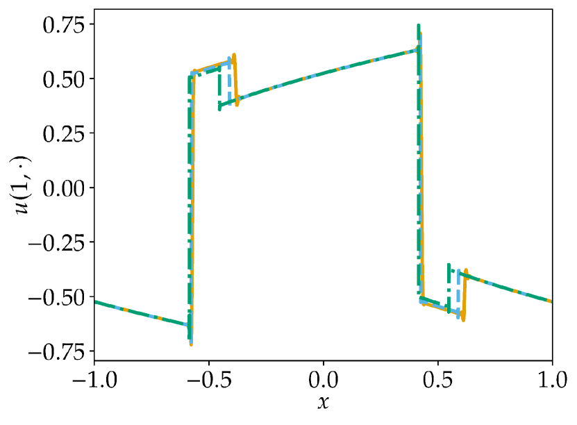
(a) Before postprocessing.

(b) After postprocessing.

Figure 2: Numerical solutions shown in 3(a) before and after postprocessing.

Using the split form and second-order artificial dissipation, the numerical solutions seem to converge to the classical entropy solution (3(a)). However, if artificial dissipation operators approximating higher-order-derivatives are used, nonclassical shocks appear in the numerical solutions (3(c) and 3(e)). The nonclassical parts of the numerical solutions become smaller for increased number of grid points but are still clearly visible even for $N=2^{14}=$16\,384$$ nodes, which seems to be pretty much for a relatively simple problem in one space dimension. Increasing the strength $\varepsilon$ of the artificial dissipation operators of higher order does not yield substantially better results, the nonclassical parts remain (not plotted). In accordance with the theory of nonclassical shocks of LeFloch [38, 39] and the entropy rate admissibility criterion of Dafermos [9], the final entropy of the classical solutions is smaller than the final entropy of the numerical solutions containing nonclassical shocks.

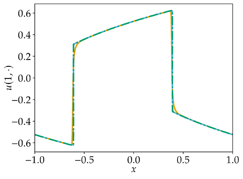
(a) Split form, second-order dissipation, $\varepsilon=400$; numerical solutions at $t=1$.

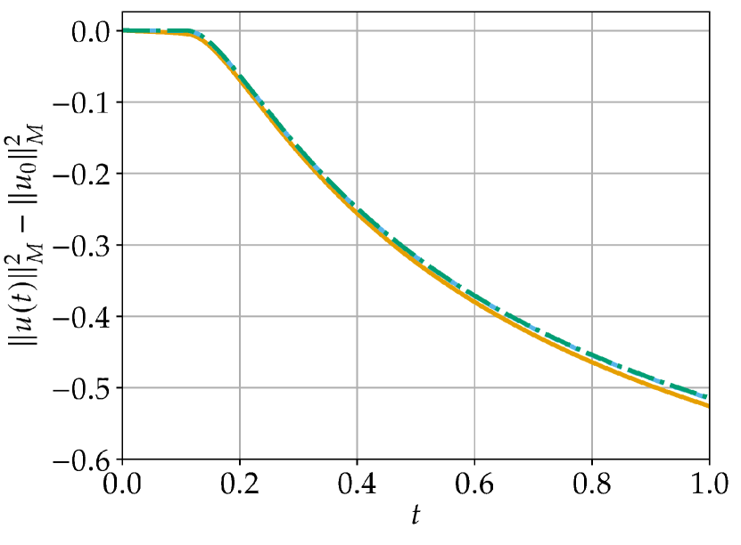
(b) Split form, second-order dissipation, $\varepsilon=400$; evolution of the $L^{2}$ entropy.

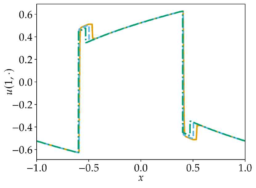
(c) Split form, fourth-order dissipation, $\varepsilon=400$; numerical solutions at $t=1$.

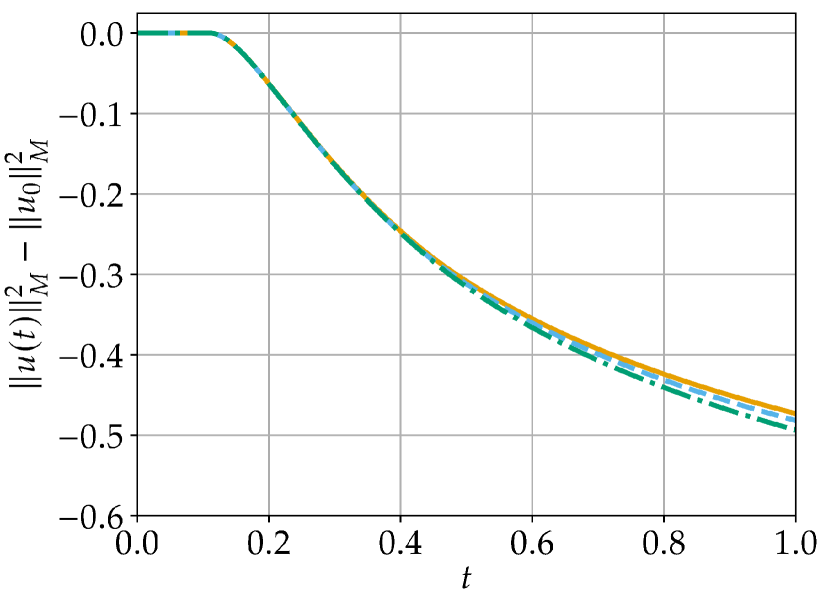
(d) Split form, fourth-order dissipation, $\varepsilon=400$; evolution of the $L^{2}$ entropy.

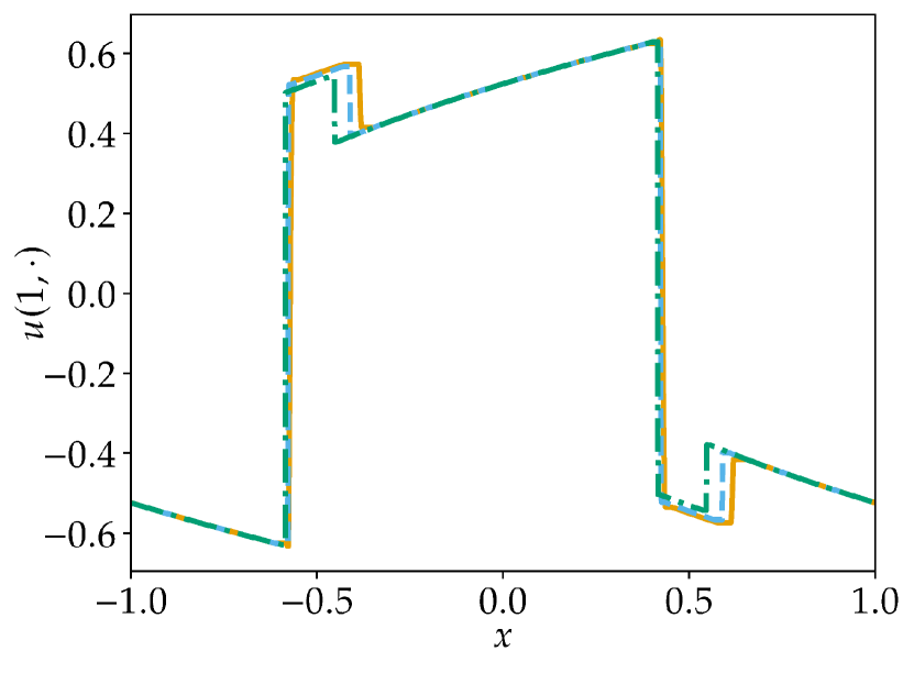
(e) Split form, sixth-order dissipation, $\varepsilon=400$; numerical solutions at $t=1$.

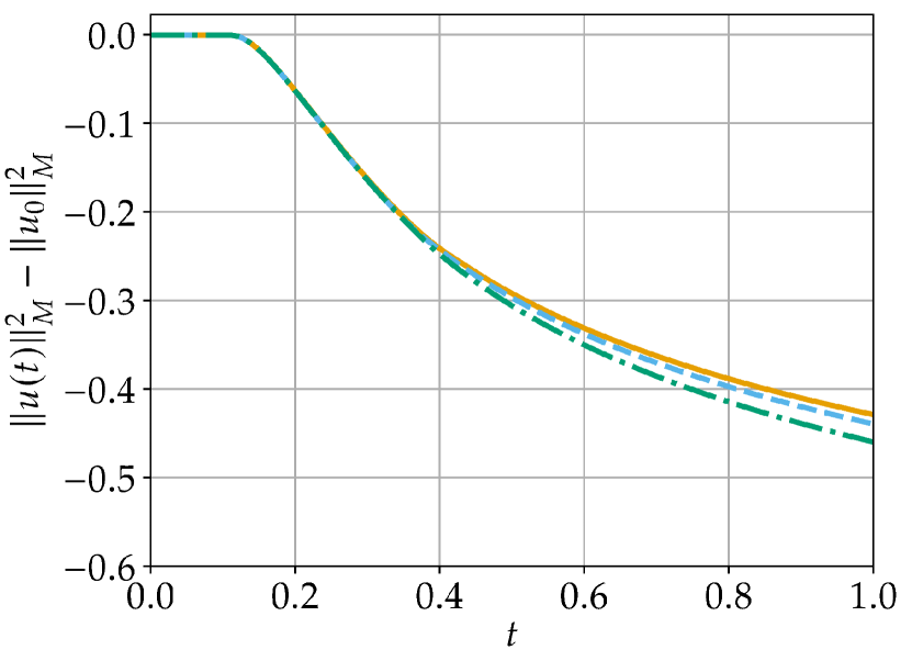
(f) Split form, sixth-order dissipation, $\varepsilon=400$; evolution of the $L^{2}$ entropy.

Figure 3: Numerical results for periodic finite differences using the split form (18) in order to approximate solutions of the cubic conservation law (16) with dissipation operators of different degrees for $N=1024$ (solid), $N=4096$ (dashed), and $N=$16\,384$$ (dotted) grid points.

Using the unsplit form, similar numerical results are obtained (Figure 4). Nevertheless, there are some important differences. Firstly, while the numerical solutions with $N=2^{10}$ and $N=2^{12}$ nodes and second-order artificial dissipation seem to be classical, small regions containing nonclassical shocks appear for $N=2^{14}=$16\,384$$ nodes (4(a)). Moreover, the nonclassical parts of the numerical solutions for higher-order artificial dissipation do not seem to become smaller at the same rate as for the split form (18). In fact, using fourth-order dissipation operators, the numerical solutions for $N=2^{12}=$4096$$ and $N=2^{14}=$16\,384$$ nodes are visually nearly indistinguishable (4(c)).

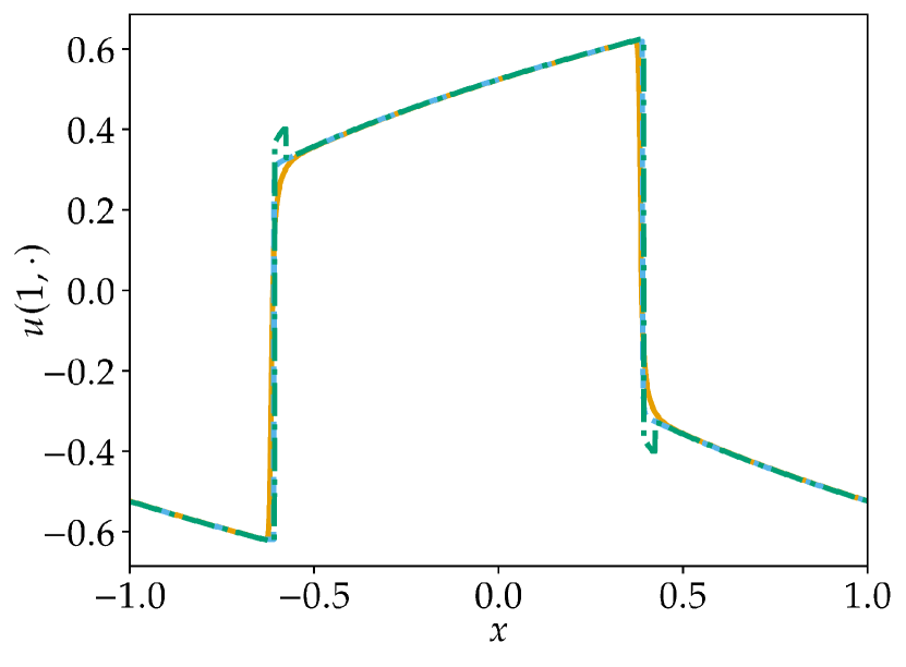
(a) Unsplit form, second-order dissipation, $\varepsilon=400$; numerical solutions at $t=1$.

(b) Unsplit form, second-order dissipation, $\varepsilon=400$; evolution of the $L^{2}$ entropy.

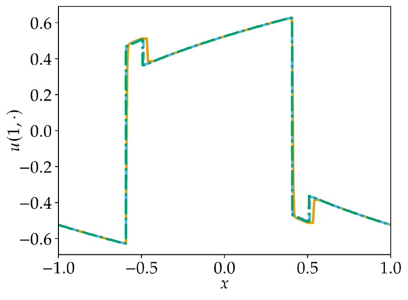
(c) Unsplit form, fourth-order dissipation, $\varepsilon=400$; numerical solutions at $t=1$.

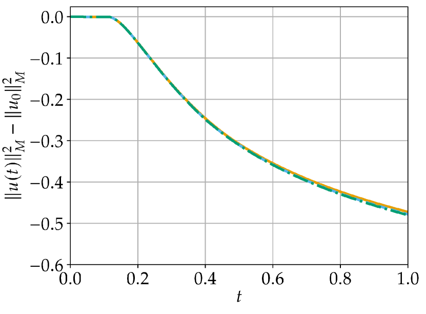
(d) Unsplit form, fourth-order dissipation, $\varepsilon=400$; evolution of the $L^{2}$ entropy.

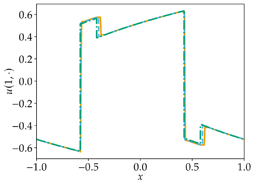
(e) Unsplit form, sixth-order dissipation, $\varepsilon=400$; numerical solutions at $t=1$.

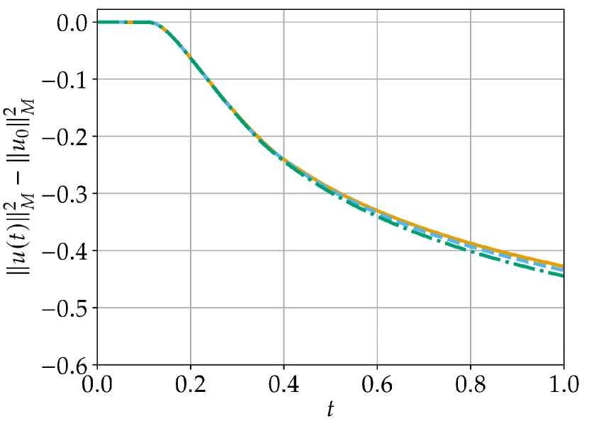
(f) Unsplit form, sixth-order dissipation, $\varepsilon=400$; evolution of the $L^{2}$ entropy.

Figure 4: Numerical results for periodic finite differences using the unsplit form (19) in order to approximate solutions of the cubic conservation law (16) with dissipation operators of different degrees for $N=1024$ (solid), $N=4096$ (dashed), and $N=$16\,384$$ (dotted) grid points.

Results of the numerical experiments using entropy-stable Fourier methods are shown in Figure 5. Using the “standard” dissipation (20), the numerical solutions for $N\in\{2^{10},2^{12},2^{14}\}$ are visually indistinguishable and include nonclassical shocks (5(a)). Using the “convergent” choice (21) of the dissipation coefficients with strength $\varepsilon=\frac{1}{N}$, the numerical solutions still contain nonclassical shocks but these nonclassical regions become smaller for increasing numbers of grid points $N$ (5(c)). However, nonclassical shocks are still visible even for $N=2^{14}=$16\,384$$ nodes, which seems to be a very high resolution for this one-dimensional problem. Again, the final total entropy becomes smaller as the nonclassical regions become smaller. Surprisingly, reducing the strength of the spectral viscosity operators to $\varepsilon=\frac{1}{5N}$, the convergence to the classical entropy solution becomes faster and more clearly visible (5(e)). Thus, reducing the strength $\varepsilon$ of the artificial dissipation increases the total dissipation, since the classical solution is approached and the final value of the total entropy is smaller than for nonclassical solutions.

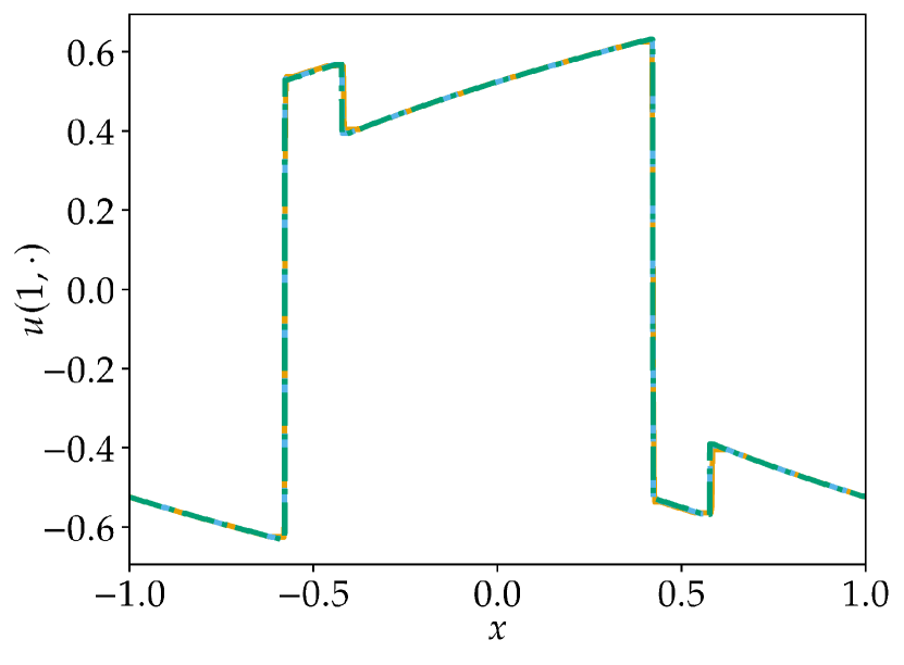
(a) “Standard” dissipation (21), $\varepsilon=\frac{1}{N}$; numerical solutions at $t=1$.

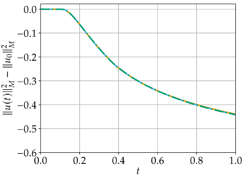
(b) “Standard” dissipation (21), $\varepsilon=\frac{1}{N}$; evolution of the $L^{2}$ entropy.

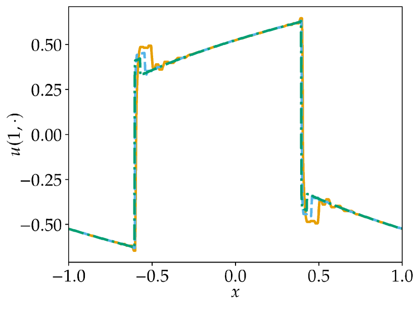
(c) “Convergent” dissipation (21), $\varepsilon=\frac{1}{N}$; numerical solutions at $t=1$.

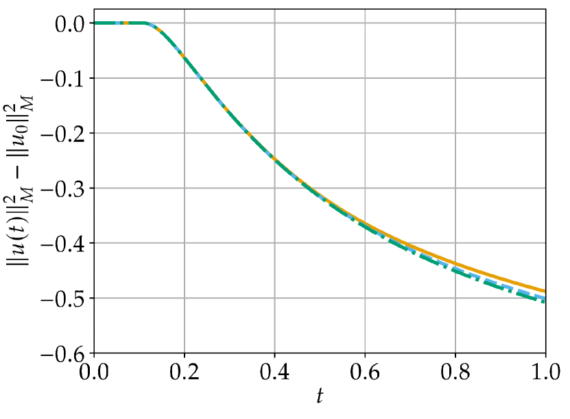
(d) “Convergent” dissipation (21), $\varepsilon=\frac{1}{N}$; evolution of the $L^{2}$ entropy.

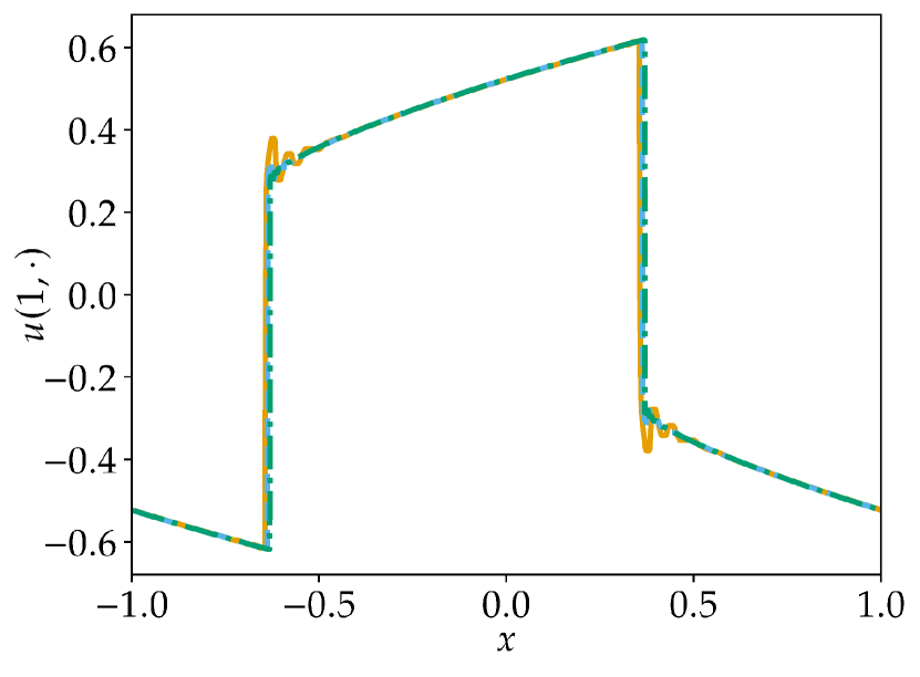
(e) “Convergent” dissipation (21), $\varepsilon=\frac{1}{5N}$; numerical solutions at $t=1$.

(f) “Convergent” dissipation (21), $\varepsilon=\frac{1}{5N}$; evolution of the $L^{2}$ entropy.

Figure 5: Numerical results for Fourier methods approximating solutions of the cubic conservation law (16) with viscosity operators of different forms and strengths for $N=1024$ (solid), $N=4096$ (dashed), and $N=$16\,384$$ (dotted) grid points.

3.2 Non-periodic boundary conditions

Considering non-periodic boundary conditions, it might be expected that a boundary condition has to be provided at the left-hand side (i.e. at ${x_{L}}$), since the advection speed $f^{\prime}(u)=3u^{2}$ is non-negative. Similarly, no boundary data should be given at the right-hand side, i.e. at ${x_{R}}$. Indeed, smooth solutions of the initial boundary value problem

$$\partial_{t}u(t,x)+\partial_{x}u(t,x)^{3} =0, t\in(0,T),\,x\in({x_{L}},{x_{R}}),$$ (22)

$$u(0,x) =u_{0}(x), x\in({x_{L}},{x_{R}}),$$

$$u(t,{x_{L}}) =g_{L}(t), t\in(0,T),$$

with compatible initial and boundary data fulfil

$$\frac{1}{2}\dfrac{\operatorname{d\!}{}}{\operatorname{d\!}{t}}\int_{x_{L}}^{x_{R}}u(t,x)^{2}\operatorname{d\!}x =\int_{x_{L}}^{x_{R}}u(t,x)\,\partial_{t}u(t,x)\operatorname{d\!}x=-\int_{x_{L}}^{x_{R}}u(t,x)\,\partial_{x}u(t,x)^{3}\operatorname{d\!}x$$ (23)

$$=-\frac{3}{4}u(t,x)^{4}\big{|}_{x_{L}}^{x_{R}}=\frac{3}{4}g_{L}(t)^{4}-\frac{3}{4}u(t,{x_{R}})^{4}.$$

Thus, the total entropy is bounded by initial and boundary data.

Considering the semi-discretization described in Theorem 2.11 results in the semi-discrete entropy balance

$$\dfrac{\operatorname{d\!}{}}{\operatorname{d\!}{t}}\mathinner{\!\left\lVert\underline{u}\right\rVert}_{M}^{2} =\underline{u}^{T}\underline{\underline{M}}\,\partial_{t}\underline{u}=\bigl{(}u_{L}f^{\mathrm{num}}_{L}-\frac{1}{4}u_{L}^{4}\bigr{)}-\bigl{(}u_{R}f^{\mathrm{num}}_{R}-\frac{1}{4}u_{R}^{4}\bigr{)},$$ (24)

in which $\frac{1}{4}u_{L}^{4}=\psi_{L}$ and $\frac{1}{4}u_{R}^{4}=\psi_{R}$. Using Godunov’s flux $f^{\mathrm{num}}(u_{-},u_{+})=u_{-}^{3}$ yields

$$\dfrac{\operatorname{d\!}{}}{\operatorname{d\!}{t}}\mathinner{\!\left\lVert\underline{u}\right\rVert}_{M}^{2}=\biggl{(}u_{L}g_{L}^{3}-\frac{1}{4}u_{L}^{4}\biggr{)}-\biggl{(}u_{R}^{4}-\frac{1}{4}u_{R}^{4}\biggr{)}\\ =\frac{3}{4}g_{L}^{4}-\frac{3}{4}u_{R}^{4}-\frac{1}{4}\underbrace{(u_{L}-g_{L})^{2}\bigl{(}3g_{L}^{2}+2u_{L}g_{L}+u_{L}^{2}\bigr{)}}_{\geq 0},$$ (25)

since

$$0 \leq(u_{L}-g_{L})^{2}\bigl{(}3g_{L}^{2}+2u_{L}g_{L}+u_{L}^{2}\bigr{)}$$ (26)

$$=3u_{L}^{2}g_{L}^{2}+2u_{L}^{3}g_{L}+u_{L}^{4}-6u_{L}g_{L}^{3}-4u_{L}^{2}g_{L}^{2}-2u_{L}^{3}g_{L}+3g_{L}^{4}+2u_{L}g_{L}^{3}+u_{L}^{2}g_{L}^{2}$$

$$=u_{L}^{4}-4u_{L}g_{L}^{3}+3g_{L}^{4}.$$

Thus, the entropy rate of the numerical solution is bounded from above by the corresponding analytical entropy rate. Hence, using Godunov’s flux at the (exterior) boundaries results in an entropy-stable scheme. If multiple elements are used, the numerical flux at inter-element boundaries can be any entropy-stable flux (cf. Definition 2.8), resulting in entropy-stable semi-discretizations.

In the following, homogeneous boundary data $g_{L}(t)\equiv 0$ and the initial condition $u_{0}(x)=-\sin(\pi x)$ will be used. The domain $({x_{L}},{x_{R}})=(-1,3)$ is divided uniformly into $N$ elements. A DG approach on Lobatto nodes is used, i.e. the solution is represented on each element as a polynomial of degree $\leq p$, represented in a nodal basis. Godunov’s flux is used both at the exterior and the interior boundaries. Moreover, the entropy-conservative flux (17) is used for the volume terms as described in Theorem 2.11. Again, SSPRK(10,4) is used to advance the numerical solutions in time, up to the final time $T=1.5$. The time step is chosen as $\Delta t=\frac{1}{N(p^{2}+1)}$.

Results of the numerical experiments are visualized in Figure 6, where numerical solutions at the final time $T$ are shown at the left-hand side. On the right-hand side, the evolution of the discrete total entropy $\mathinner{\!\left\lVert\underline{u}\right\rVert}_{M}^{2}$ (summed over all elements) is visualized. Here, the mass matrix $\underline{\underline{M}}\,$ is a diagonal matrix containing the Lobatto Legendre quadrature weights on the diagonal, scaled by an appropriate factor to account for the width of each cell.

The numerical solutions for the same polynomial degree $p$ are visually nearly indistinguishable. Using polynomials of degree $p=1$, the numerical solutions converge to the classical entropy solution (6(a)). If polynomials of higher degree $p\geq 2$ are used, nonclassical shocks develop and remain stable and unchanged if the number of elements is increased. As in the periodic case, the final value of the total entropy is higher if nonclassical shocks occur.

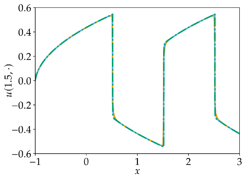
(a) Polynomial degree $p=1$; numerical solutions at $t=1.5$.

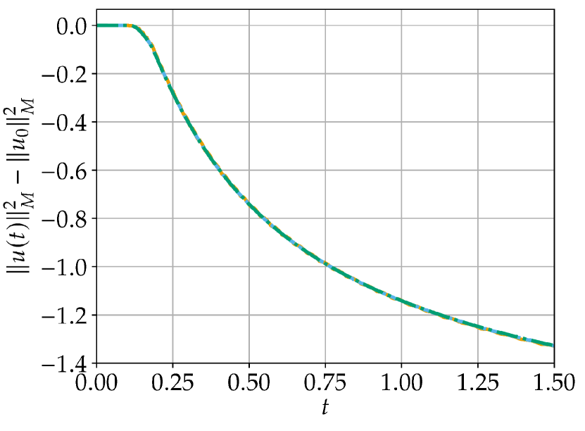
(b) Polynomial degree $p=1$; evolution of the $L^{2}$ entropy.

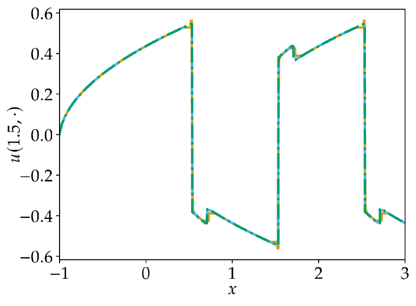
(c) Polynomial degree $p=2$; numerical solutions at $t=1.5$.

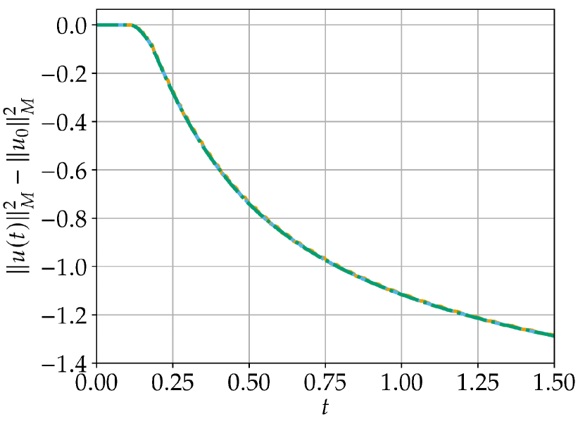
(d) Polynomial degree $p=2$; evolution of the $L^{2}$ entropy.

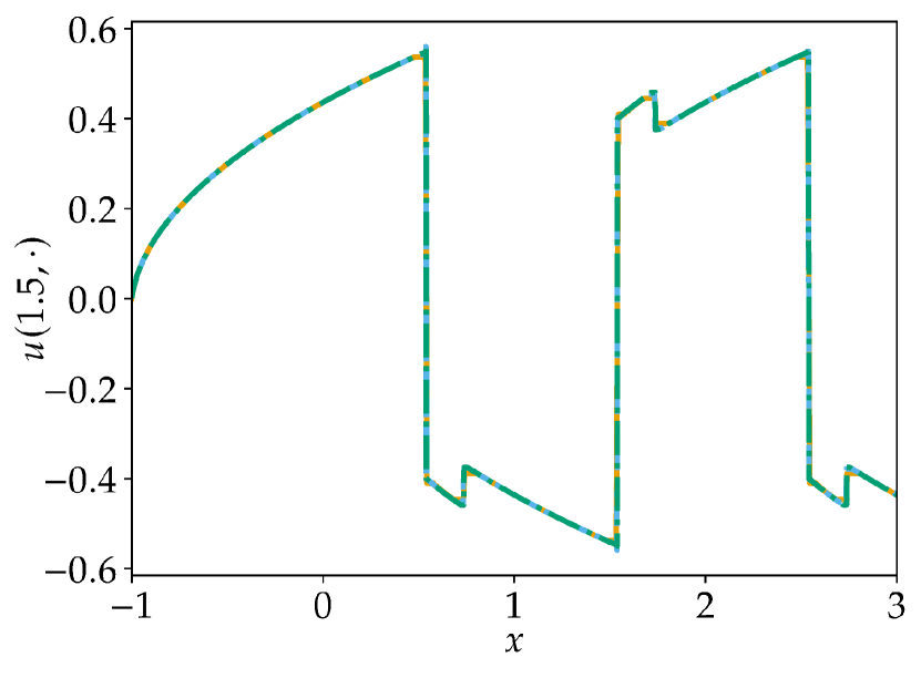
(e) Polynomial degree $p=3$; numerical solutions at $t=1.5$.

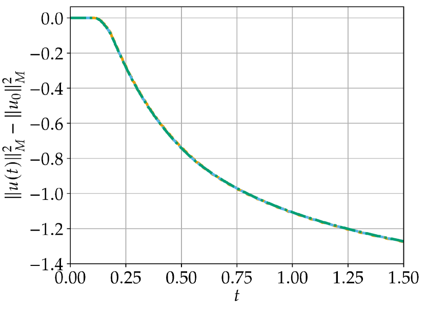
(f) Polynomial degree $p=3$; evolution of the $L^{2}$ entropy.

Figure 6: Numerical results for DG methods using Godunov’s flux and the entropy stable semi-discretization of Theorem 2.11 in order to approximate solutions of the cubic conservation law (22) with different polynomial degrees $p$ for $N=256$ (solid), $N=1024$ (dashed), and $N=4096$ (dotted) elements.

Introducing another kind of dissipation (besides the dissipation provided by the numerical fluxes as in the previous examples), modal filtering is applied after every complete time step of the Runge-Kutta method. This modal filtering can be seen as a discretization of the $s$th power of the Legendre dissipation operator, cf. Example 2.17. Here, the strength $\varepsilon$ is chosen as $\varepsilon=-\log(\mathtt{eps})/(\Delta t\,(n(n+1))^{s})$, where $\mathtt{eps}$ is the machine accuracy, i.e. $\mathtt{eps}=$2.220\,446\,049\,250\,313\text{\times}{10}^{-16}$$ for $64$ bit floating point numbers (Float64 in Julia [2]) used in the calculations.

Results of the numerical experiments using DG methods with modal filtering of different orders $s$ are shown in Figure 7. The numerical solutions using different numbers $N$ of elements are visually nearly indistinguishable. Using the filter order $s=1$, the numerical solutions converge to the classical entropy weak solution (7(a)). However, if the filter order is increased, the numerical solutions converge to nonclassical solutions (7(c) and 7(e)). As before, the appearance of nonclassical shocks is linked with less entropy dissipation.

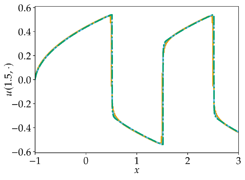
(a) Filter order $s=1$; numerical solutions at $t=1.5$.

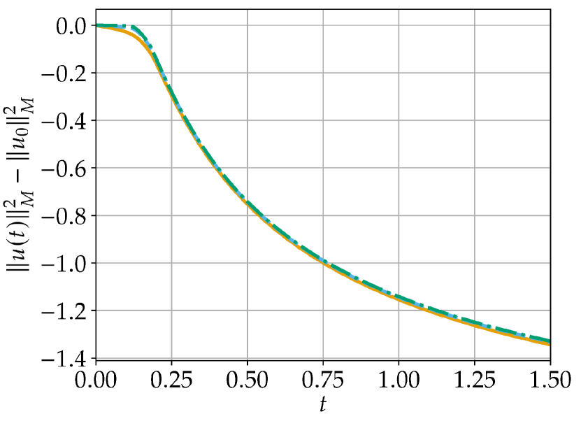
(b) Filter order $s=1$; evolution of the $L^{2}$ entropy.

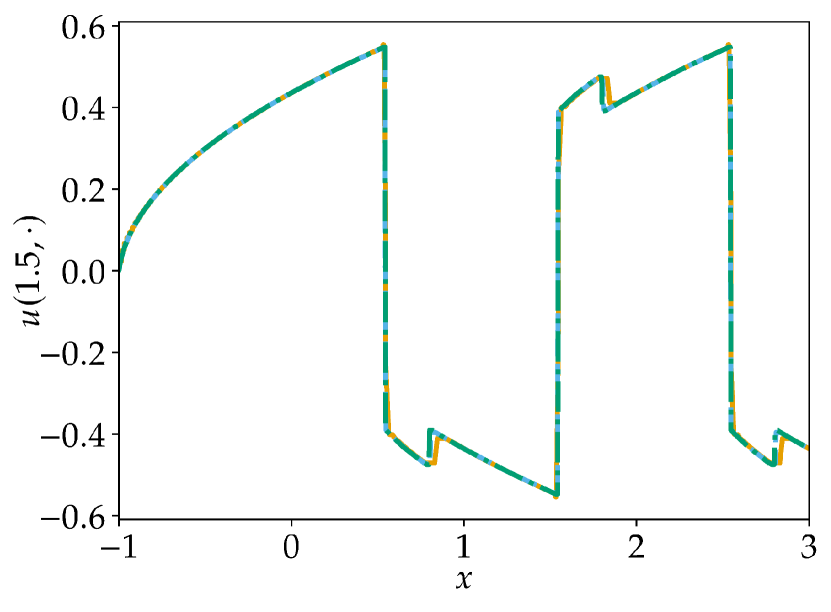
(c) Filter order $s=4$; numerical solutions at $t=1.5$.

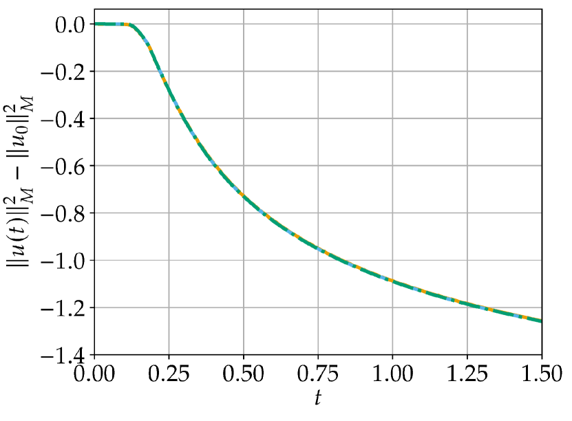
(d) Filter order $s=4$; evolution of the $L^{2}$ entropy.

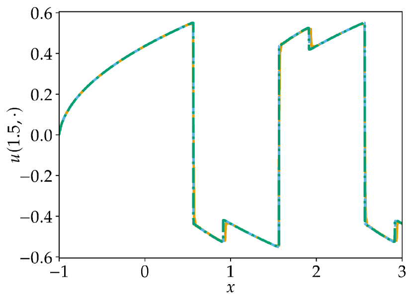
(e) Filter order $s=5$; numerical solutions at $t=1.5$.

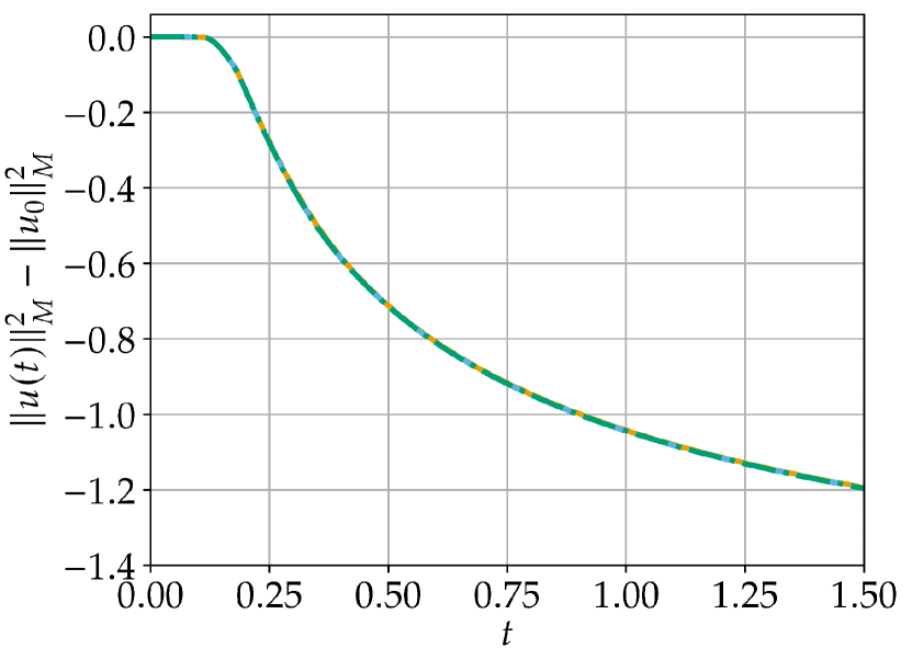
(f) Filter order $s=5$; evolution of the $L^{2}$ entropy.

Figure 7: Numerical results for DG methods using Godunov’s flux and the entropy stable semi-discretization of Theorem 2.11 in order to approximate solutions of the cubic conservation law (22) with polynomial degree $p=4$ and different filter orders $s$ for $N=256$ (solid), $N=1024$ (dashed), and $N=4096$ (dotted) elements.

Furthermore, finite difference SBP methods with the same boundary procedures as the DG schemes are tested as well. The results using only a single kind of artificial dissipation operator are similar to the ones in the periodic case and thus not shown here. Instead, the artificial dissipation operators of [50] are weighted with strengths $\varepsilon_{2}$ (second-order dissipation), $\varepsilon_{4}$ (fourth-order dissipation), and $\varepsilon_{6}$ (sixth-order dissipation) and added to the semi-discretization. The time step is chosen as $\Delta t=\frac{1}{N}$. The results of these numerical experiments are presented in Figure 8. As can be seen there, for a fixed choice of the strengths $\varepsilon_{i}$, nonclassical shocks occur under grid refinement. Thus, the influence of the higher-order dissipation operators can destroy the convergence to the classical solution induced by the second-order dissipation operator.

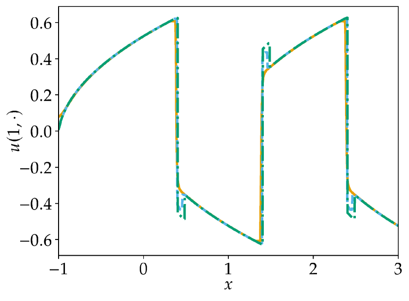
(a) Dissipation strengths $\varepsilon_{2}=100$, $\varepsilon_{4}=100$, $\varepsilon_{6}=100$; numerical solutions at $t=1.5$.

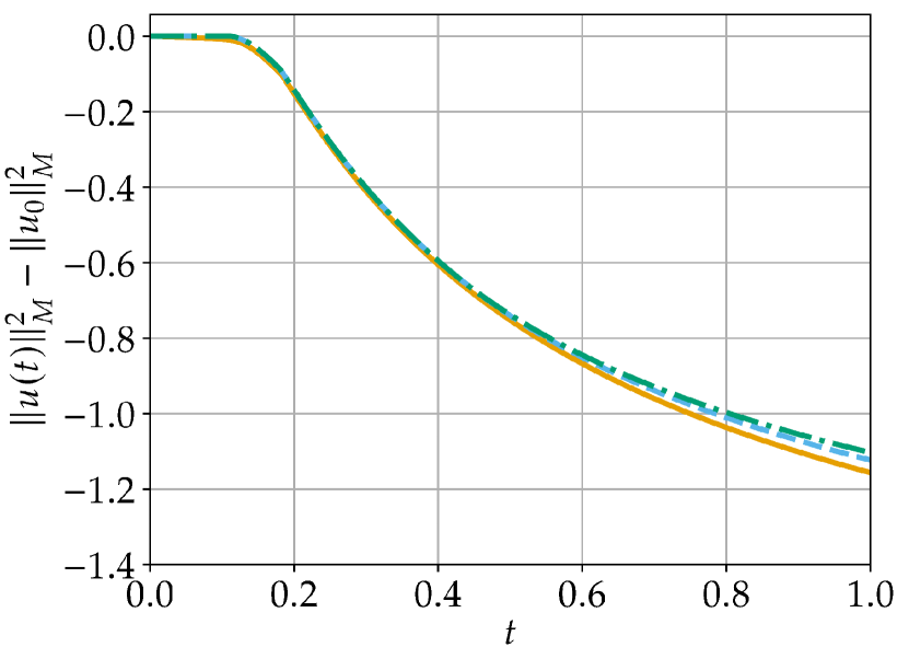
(b) Dissipation strengths $\varepsilon_{2}=100$, $\varepsilon_{4}=100$, $\varepsilon_{6}=100$; evolution of the $L^{2}$ entropy.

(c) Dissipation strengths $\varepsilon_{2}=0$, $\varepsilon_{4}=100$, $\varepsilon_{6}=100$; numerical solutions at $t=1.5$.

(d) Dissipation strengths $\varepsilon_{2}=0$, $\varepsilon_{4}=100$, $\varepsilon_{6}=100$; evolution of the $L^{2}$ entropy.

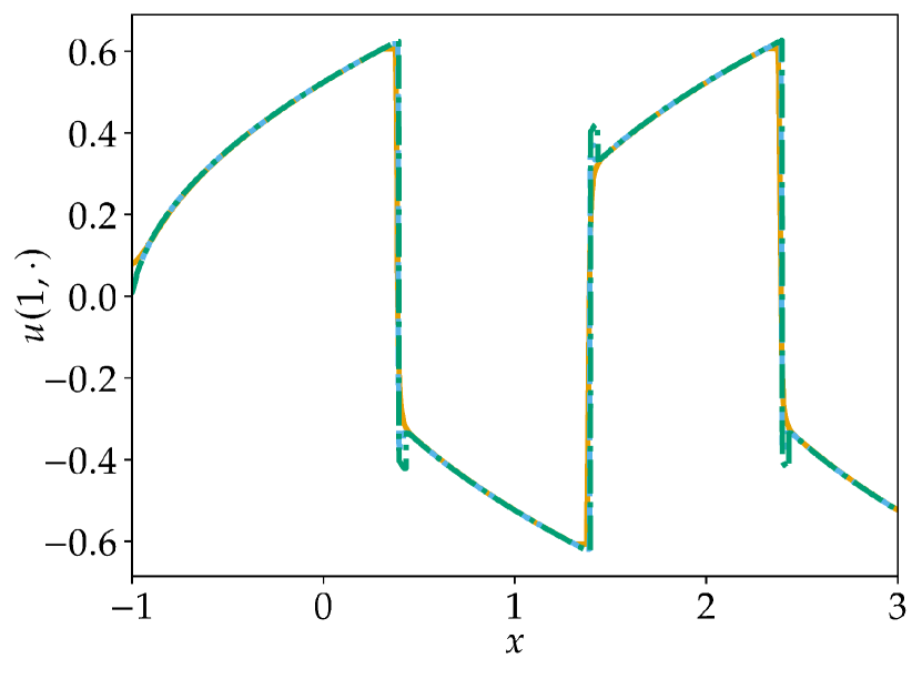
(e) Dissipation strengths $\varepsilon_{2}=100$, $\varepsilon_{4}=100$, $\varepsilon_{6}=0$; numerical solutions at $t=1.5$.

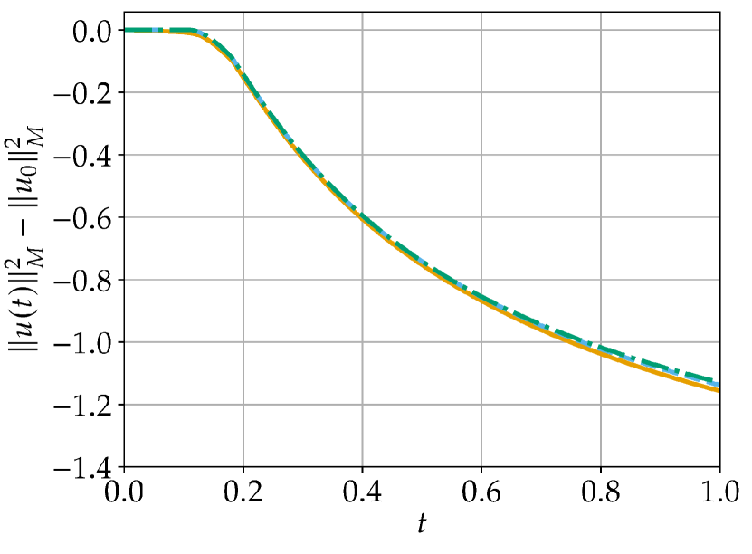
(f) Dissipation strengths $\varepsilon_{2}=100$, $\varepsilon_{4}=100$, $\varepsilon_{6}=0$; evolution of the $L^{2}$ entropy.

Figure 8: Numerical results for SBP FD methods with interior order of accuracy six using Godunov’s flux at the boundaries and the entropy-stable semi-discretization of Theorem 2.11 in order to approximate solutions of the cubic conservation law (22) with different artificial dissipation operators for $N=1024$ (solid), $N=4096$ (dashed), and $N=$16\,384$$ (dotted) grid points.

4 Uniqueness and entropy properties for the cubic conservation law

4.1 Preliminaries

Here, the TeCNO schemes in [16, 14] mentioned in Example 2.16 are now used to compute numerical solutions of the cubic conservation law (16) with periodic boundary conditions. As in the Section 3, the initial condition is chosen as $u_{0}(x)=-\sin(\pi x)$ in the domain $({x_{L}},{x_{R}})=(-1,1)$ and the numerical solutions are evolved up to the final time $T=1$ using the fourth-order, ten stage, strong stability preserving explicit Runge-Kutta method SSPRK(10,4) of [29] with time steps $\Delta t=1/N$. The following entropy functions will be considered.

• The $L^{2}$ entropy $U(u)=\frac{1}{2}u^{2}$. As in Section 3, the entropy variables are $w(u)=U^{\prime}(u)=u$ and the flux potential is $\psi(u)=\frac{1}{4}u^{4}$. Thus, the corresponding entropy-conservative numerical flux is (17).

• The $L^{4}$ entropy $U(u)=\frac{1}{4}u^{4}$. In this case, $w(u)=U^{\prime}(u)=u^{3}$ and the flux potential is $\psi(u)=\frac{1}{2}u^{6}$. Hence, the entropy-conservative numerical flux is the central flux $f^{\mathrm{num}}(u_{-},u_{+})=\frac{\psi(u_{+})-\psi(u_{-})}{w(u_{+})-w(u_{-})}=\frac{u_{+}^{3}+u_{-}^{3}}{2}.$

• The $L^{2}\cap L^{4}$ entropy $U(u)=\frac{1}{4}u^{4}+\frac{\alpha}{2}u^{2}$, $\alpha>0$. For this strictly convex entropy, $w(u)=U^{\prime}(u)=u^{3}+\alpha u$ and $\psi(u)=\frac{1}{2}u^{6}+\frac{\alpha}{4}u^{4}$. The corresponding entropy-conservative numerical flux is

  $$\quad f^{\mathrm{num}}(u_{-},u_{+})=\frac{1}{2}\frac{u_{+}^{6}-u_{-}^{6}+\frac{\alpha}{2}u_{+}^{4}-\frac{\alpha}{2}u_{-}^{4}}{u_{+}^{3}-u_{-}^{3}+\alpha u_{+}-\alpha u_{-}}$$ (27)

  $$=\frac{1}{2}\frac{u_{+}^{5}+u_{+}^{4}u_{-}+u_{+}^{3}u_{-}^{2}+u_{+}^{2}u_{-}^{3}+u_{+}u_{-}^{4}+u_{-}^{5}+\frac{\alpha}{2}\bigl{(}u_{+}^{3}+u_{+}^{2}u_{-}+u_{+}u_{-}^{2}+u_{-}^{3}\bigr{)}}{u_{+}^{2}+u_{+}u_{-}+u_{-}^{2}+\alpha},$$

  where the fraction has been reduced by $(u_{+}-u_{-})$. In the numerical experiments presented in the following, $\alpha=\frac{1}{100}$ has been chosen.

4.2 Numerical results

Results of numerical experiments with TeCNO(3) schemes can be seen in Figure 9. For the schemes based on the $L^{2}$ entropy, the numerical solutions are visually indistinguishable from the entropy weak solution. In contrast, the schemes based on the $L^{4}$ entropy yield numerical solutions with overshoots at the discontinuities that do not vanish as the grid is refined. Results using TeCNO(2) schemes are similar; the overshoot regions are a bit smaller but clearly present for all investigated numbers $N$ of cells. It might be conjectured that the “better” behavior of the schemes based on the $L^{2}$ entropy $U(u)=\frac{1}{2}u^{2}$ compared to the $L^{4}$ entropy $U(u)=\frac{1}{4}u^{4}$ is influenced by the fact that the former entropy is strictly convex while the latter is only convex. However, the schemes based on the strictly convex $L^{2}\cap L^{4}$ entropy show the same behavior as the ones based on the $L^{4}$ entropy, i.e. the overshoots persist.

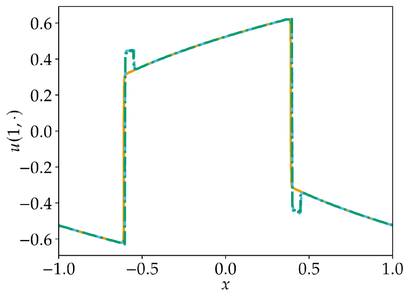
(a) $N=2^{10}=$1024$$; numerical solutions at $t=1$.

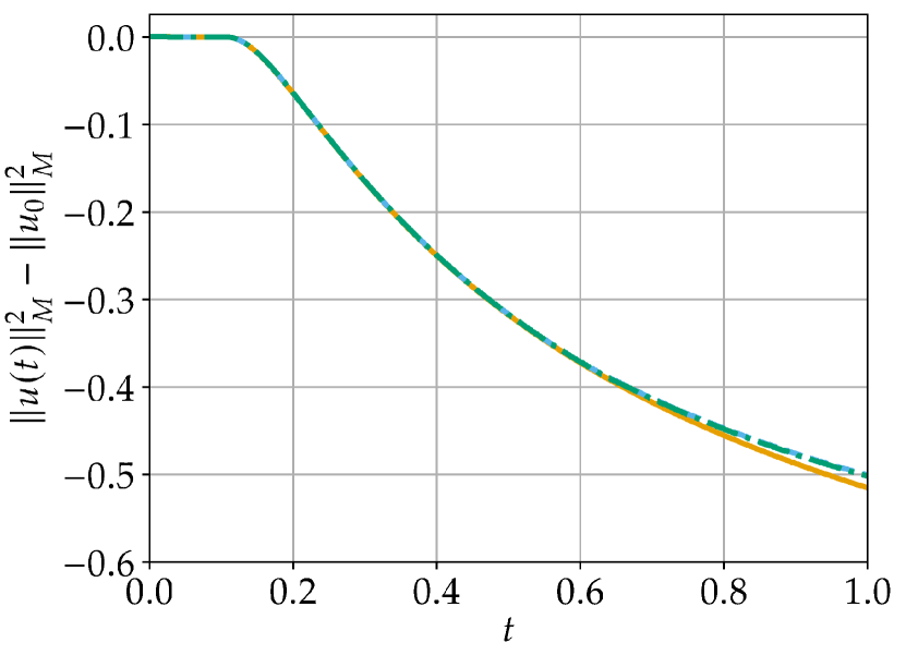
(b) $N=2^{10}=$1024$$; evolution of the $L^{2}$ entropy.

(c) $N=2^{12}=$4096$$; numerical solutions at $t=1$.

(d) $N=2^{12}=$4096$$; evolution of the $L^{2}$ entropy.

(e) $N=2^{14}=$16\,384$$; numerical solutions at $t=1$.

(f) $N=2^{14}=$16\,384$$; evolution of the $L^{2}$ entropy.

Figure 9: Numerical results for TeCNO(3) methods approximating solutions of the cubic conservation law (16) based on different entropy functions for $N$ of cells.

5 Computing kinetic functions numerically

5.1 Preliminaries

To analyze the behavior of the provably entropy-dissipative numerical methods described above in more detail, the corresponding kinetic functions will be computed. The basic motivation is as follows [39, Chapter II]. The locally smooth parts of a weak solution of a nonlinear scalar conservation law are unique but non-uniqueness can arise from discontinuities if the flux is non-convex and only a single entropy inequality is required. Hence, an approach to single out one specific weak solutions among all weak solutions satisfying a single entropy inequality is given by prescribing the allowed forms of discontinuities. This is exactly the purpose of kinetic functions [39, Chapter II].

Consider a scalar nonlinear conservation law $\partial_{t}u+\partial_{x}f(u)=0$ in one space dimension and a weak solution of an associated Riemann problem with left- and right-hand states $u_{L}$ and $u_{R}$. This weak solution is a combination of rarefaction waves, classical shock waves (satisfying all entropy inequalities locally), and nonclassical shock waves (which are only required to satisfy a single entropy inequality locally). In this context, the kinetic function $\varphi^{\flat}$ is the mapping of the left state $u_{L}$ to the middle state $u_{M}$ if a nonclassical solution appears. We use the following definition of a kinetic function in the context of numerical solutions.

Definition 5.1.

Given a numerical solution of a Riemann problem with left- and right-hand states $u_{L}$ and $u_{R}$, define $\Upsilon_{L}\subseteq\mathbb{R}$ as the set of all left-hand states $u_{L}$ such that the numerical solution results contains an (approximately) constant part with value $u_{M}$ that increases the total variation and is (approximately) connected to the left-hand state via a single discontinuity. The kinetic function associated to the numerical method is the mapping $\varphi^{\flat}\colon\Upsilon_{L}\to\mathbb{R}$, $\varphi^{\flat}(u_{L})=u_{M}$.

Here, a series of Riemann problems with right-hand state $u_{R}=-2$ and varying left-hand state $u_{L}$ has been solved for each scheme. The FD SBP and DG methods use a domain $[-1,3]$ with initial discontinuity located at $x=-0.5$. The solution is computed until $t=5/\max\{3u_{0}^{2}\}$ with a time step of $\Delta t=((p^{2}+1)N\max\{3u_{0}^{2}\})^{-1}$ for DG methods and $\Delta t=(N\max\{3u_{0}^{2}\})^{-1}$ for FD methods.

The Fourier methods use a domain $[-6,6]$ with initial value

$$u_{0}(x)=u_{L}\,\text{ for }x\in[-4.5,0],\,\text{ while }u_{0}(x)=u_{R}\,\text{otherwise}.$$ (28)

Again, the time step is $\Delta t=(N\max\{3u_{0}^{2}\})^{-1}$. The other parameters are the same as described above. A typical numerical solution obtained using a DG scheme is shown in Figure 10. The middle state has been computed as follows. At first, the discontinuities are detected in a simple way by averaging the solution locally and computing the standard deviation. If there are two discontinuities of the form allowing a nonclassical middle state, its value is computed as the median of the values of the numerical solution between the two discontinuities. The general theory of nonclassical shocks predicts bounds of the kinetic function $\varphi^{\flat}$. Here, as established in [39], we have

$$\varphi^{\flat}_{0}\leq\varphi^{\flat}\leq\varphi^{\sharp},\qquad\text{where }\varphi^{\flat}_{0}(u_{L})=-u_{L}\text{ and }\varphi^{\sharp}(u_{L})=-u_{L}/2.$$ (29)

Figure 10: Numerical Riemann solution $u_{\mathrm{num}}$ (without postprocessing) with $u_{L}=5$ and $u_{R}=-2$, and a DG method with parameters: polynomial degree $p=5$, filter order $s=5$, number of elements $N=256$.

5.2 Nodal DG methods

For nodal DG methods, polynomial degrees $p\in\{0,1,\dots,5\}$, filter order $s\in\{0,1,\dots,5\}$, and numbers of elements $N\in\{2^{6},2^{7},\dots,2^{11}\}$ have been used. The following observations have been made.

1. The schemes with filter order $s\in\{1,2,3\}$ did not result in nonclassical solutions.

2. The schemes with polynomial degrees $p\in\{0,1\}$ did not result in nonclassical solutions. The schemes with polynomial degree $p=2$ resulted in nonclassical solutions only if no filtering was applied ($s=0$).

3. If the strength of the initial discontinuity is too big, no nonclassical solutions occur. For the investigated range of parameters, nonclassical solutions occurred only for $u_{L}<10$ (as a necessary criterion). Depending on the other parameters, the maximal value of $u_{L}$ for which nonclassical solution occurred can be smaller.

4. The numerically obtained kinetic functions $\varphi^{\flat}$ are affine linear. These affine linear functions remain visually indistinguishable under grid refinement by increasing the number of elements $N$. This is shown for $p=5$ and $s=5$ in Figure 11.

   

   Figure 11: Kinetic function for a DG method with polynomial degree $p=5$ and filter order $s=5$.

5. The kinetic functions depend on the polynomial degree $p$. For increasing $p$, the slope becomes steeper, i.e. smaller, since it is negative. This is shown for $s=0$ and $N=$1024$$ in Figure 12.

   

   Figure 12: Kinetic function for DG methods without filtering ($s=0$) and $N=$1024$$ elements.

6. The kinetic functions depend on the filter order $s$. For $s=5$, the slope is steeper than for $s<5$. However, there is no clear relation for the other values of $s$. For $p=5$, the slopes for $s=0$ and $s=4$ are visually indistinguishable while the slope for $s=0$ is steeper than for $s=4$ for $p=4$. This is shown for $N=$1024$$ in Figure 13.

   

   (a) $p=4$.

   

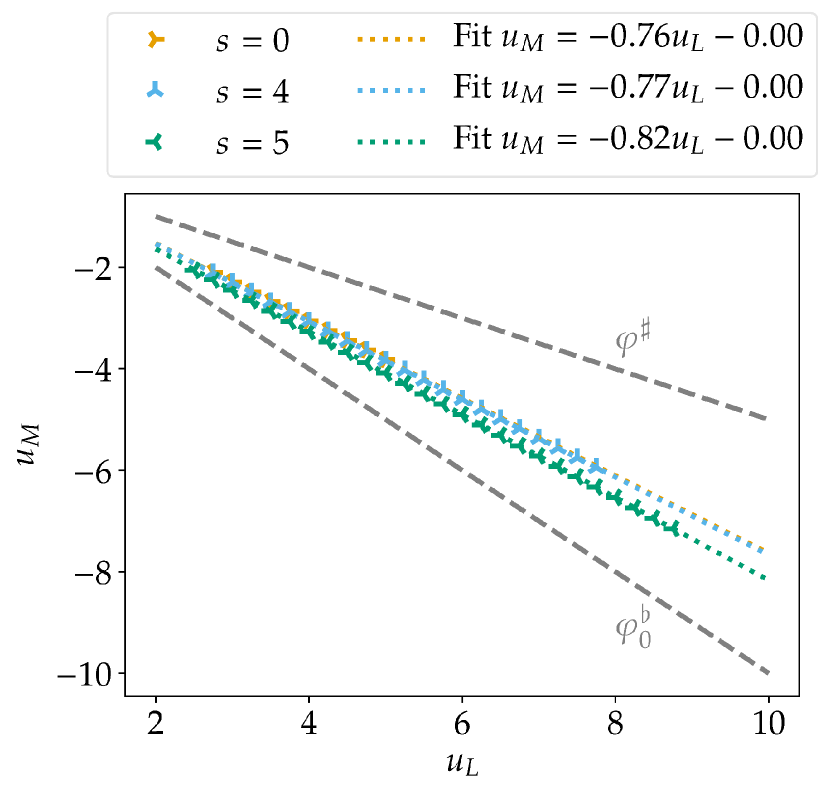
   (b) $p=5$.

   Figure 13: Kinetic function for DG methods with $N=$1024$$ elements.

7. The offset of the affine linear kinetic functions is nearly zero, i.e. the kinetic functions are approximately linear.

8. The kinetic functions satisfy the bounds (29).

5.3 Finite difference methods

For FD methods, accuracy order $p\in\{2,4,6\}$, artificial dissipation strength $\varepsilon_{i}\in\{0,100,\dots,400\}$, and $N\in\{2^{8},2^{9},\dots,2^{14}\}$ grid nodes have been used. The following observations have been made.

1. If artificial dissipation was applied, nonclassical solutions occurred at least for some values of $N$, even if only the second-order artificial dissipation was used ($\varepsilon_{2}\neq 0,\varepsilon_{4}=\varepsilon_{6}=0$). The only exception is given by the second-order method ($p=2$) with second-order artificial dissipation ($\varepsilon_{2}\neq 0$), where no nonclassical solutions occurred. This is in agreement with the results of [59]: Discretizations of the second derivative can only be entropy-dissipative for all entropies if the order of accuracy is at most two. Additionally, the second-order discretizations applied here are dissipative for all entropies. Some examples are shown in Figure 14.

   

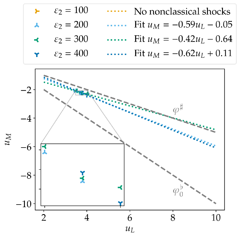
   (a) $p=4$, $\varepsilon_{4}=0$, $\varepsilon_{6}=0$.

   

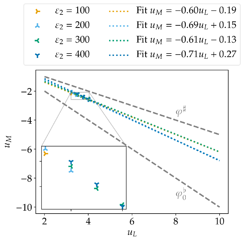
   (b) $p=6$, $\varepsilon_{4}=0$, $\varepsilon_{6}=0$.

   Figure 14: Kinetic function for FD methods with order of accuracy $p\in\{4,6\}$, $N=$4096$$ grid nodes, and different strengths of the artificial dissipation.

2. As for DG methods, if the strength of the initial discontinuity is too big, no nonclassical solutions occur. For the investigated range of parameters, nonclassical solutions occurred only for $u_{L}<10$ (as a necessary criterion). Depending on the other parameters, the maximal value of $u_{L}$ for which nonclassical solution occurred can be smaller.

3. The numerically obtained kinetic functions $\varphi^{\flat}$ are affine linear. These affine linear functions vary slightly under grid refinement but seem to converge. However, the maximal value of $u_{L}$ leading to nonclassical solutions depends on $N$ and typically decreases when $N$ is increased. This is shown in Figure 15.

   

   

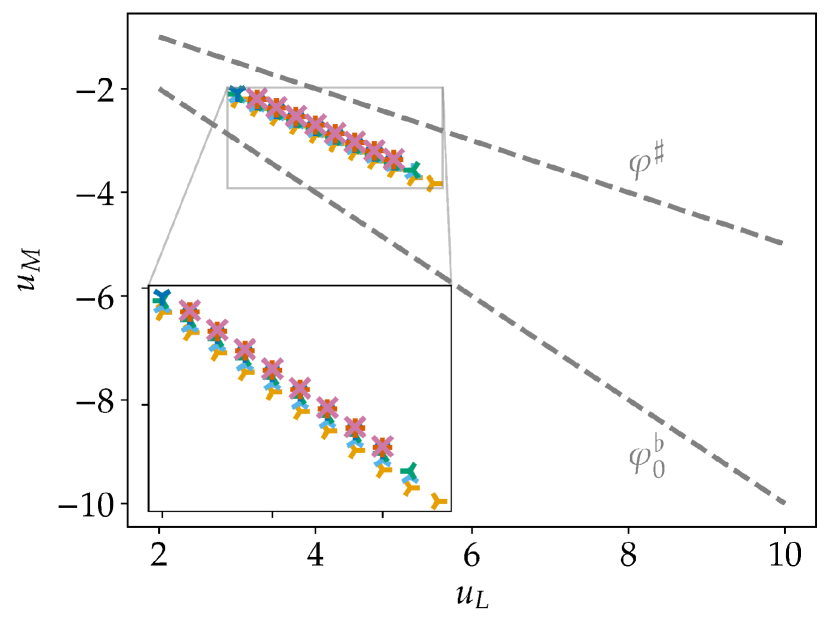
   (a) $\varepsilon_{2}=0$, $\varepsilon_{4}=400$, $\varepsilon_{6}=0$.

   

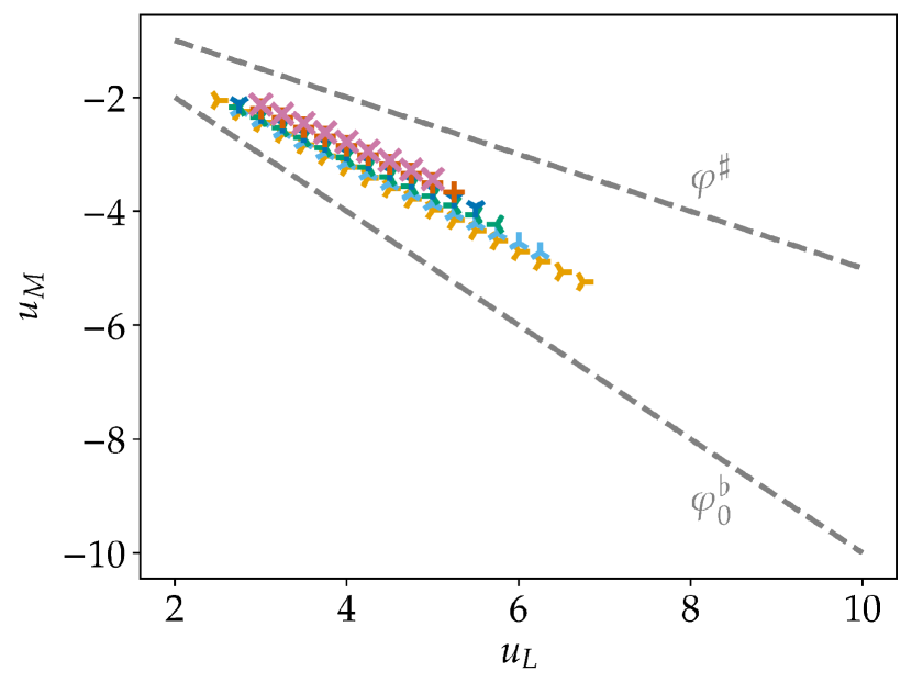
   (b) $\varepsilon_{2}=0$, $\varepsilon_{4}=0$, $\varepsilon_{6}=400$.

   Figure 15: Kinetic function for FD methods with order of accuracy $p=6$ and varying number of grid nodes $N$ for different strengths of the artificial dissipation.

4. Choosing a fixed order of the artificial dissipation, i.e. $\varepsilon_{i}\neq 0$ and $\varepsilon_{j}=0$ for $j\neq i$, the kinetic functions are nearly indistinguishable if the strength $\varepsilon_{i}\in\{100,200,300,400\}$ is varied. This is shown in Figure 16.

   

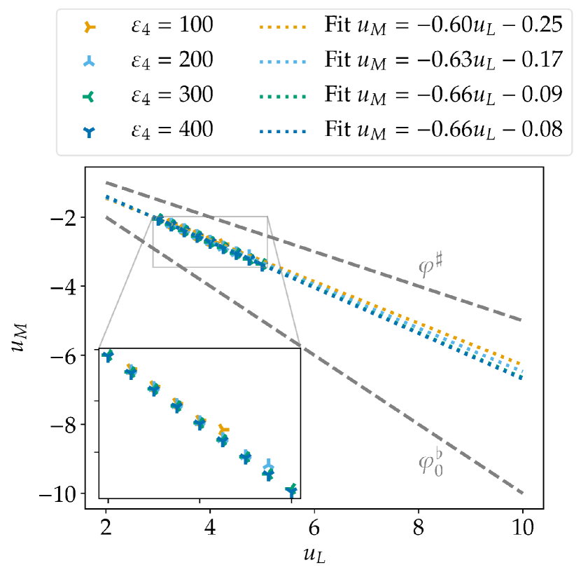
   (a) $\varepsilon_{2}=0$, $\varepsilon_{6}=0$.

   

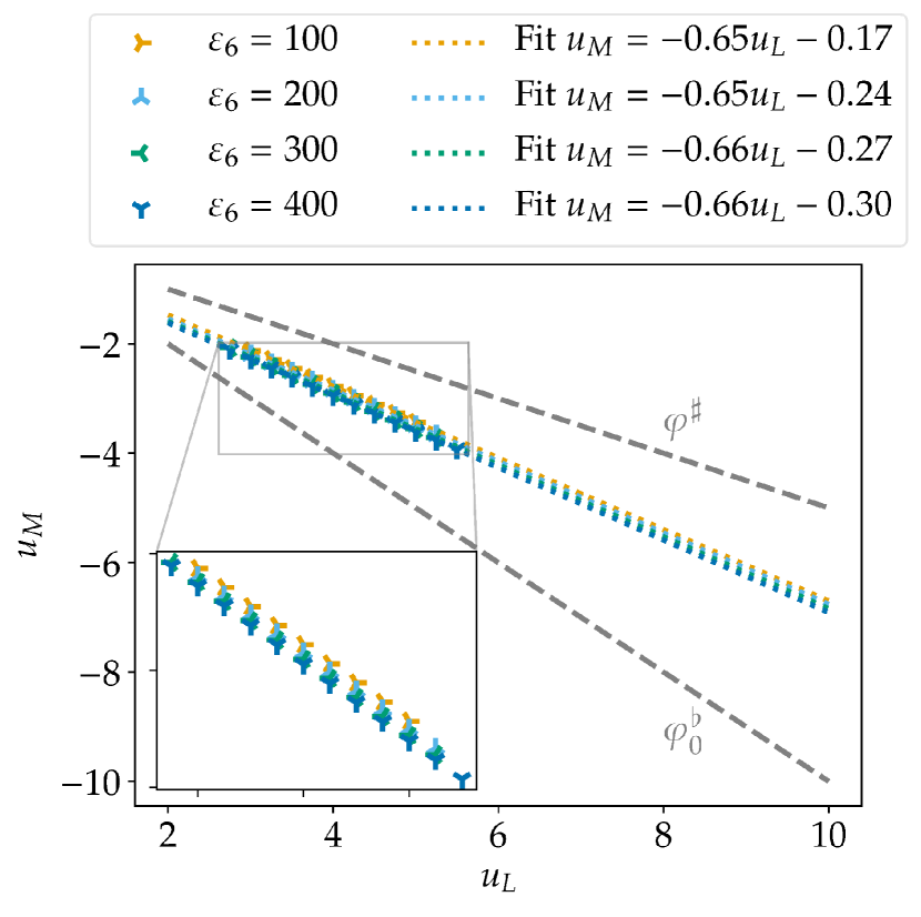
   (b) $\varepsilon_{2}=0$, $\varepsilon_{4}=0$.

   Figure 16: Kinetic function for FD methods with order of accuracy $p=6$, $N=$4096$$ grid nodes, and different strengths of the artificial dissipation.

5. The kinetic function varies with the order of accuracy $p$. Typically, it becomes steeper (more negative) for higher values of $p$. This is shown in Figure 17.

   

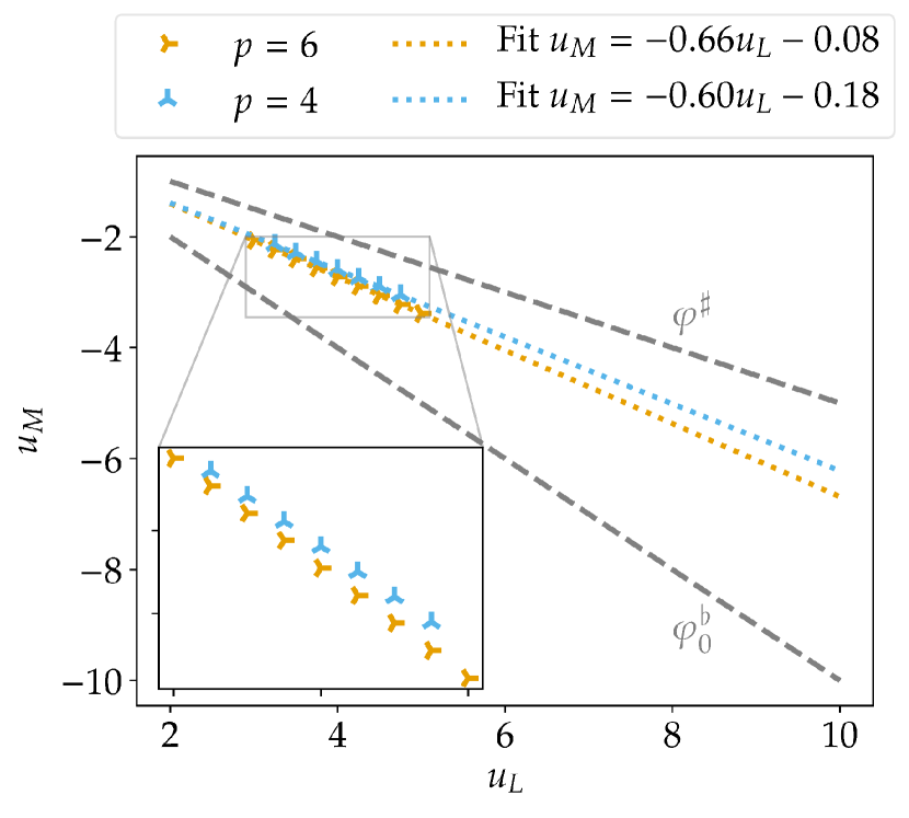
   (a) $\varepsilon_{2}=0$, $\varepsilon_{4}=400$, $\varepsilon_{6}=0$.

   

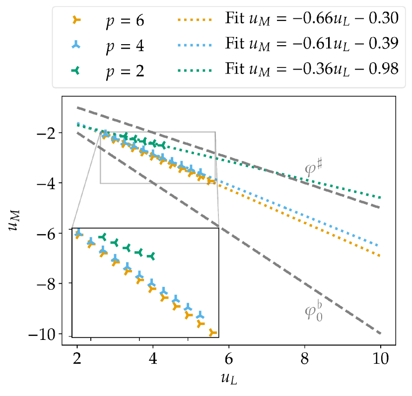
   (b) $\varepsilon_{2}=0$, $\varepsilon_{4}=0$, $\varepsilon_{6}=400$.

   Figure 17: Kinetic function for FD methods with different orders of accuracy $p$, $N=$4096$$ grid nodes, and different strengths of the artificial dissipation. For $p=2$ and $\varepsilon_{2}=0$, $\varepsilon_{4}=400$, $\varepsilon_{6}=0$, no nonclassical solutions occur.

6. In contrast to DG methods, the offset of the affine linear kinetic functions is in general not zero.

7. The kinetic functions satisfy the bounds (29) in the region where nonclassical solutions occur. For $p=2$, the kinetic functions can violate the bounds (29) if they are extrapolated to bigger values of $u_{L}$, cf. Figure 17(a). For $p\in\{4,6\}$ such a behavior did not occur.

5.4 Fourier collocation methods

For Fourier methods, the viscosity strengths $\varepsilon\in\{10/N,50/N,100/N\}$ for the standard and convergent choices of [78] and $N\in\{2^{10},2^{11},\dots,2^{14}\}$ grid nodes have been used. The following observations have been made.

1. As for DG and FD methods, if the strength of the initial discontinuity is too big, no nonclassical solutions occurred. For the investigated range of parameters, nonclassical solutions occurred only for $u_{L}<10$ (as a necessary criterion). Depending on the other parameters, the maximal value of $u_{L}$ for which nonclassical solution occurred can be smaller.

2. The numerically obtained kinetic functions $\varphi^{\flat}$ are affine linear and seem to converge under grid refinement (or are already visually indistinguishable). This can be seen in Figure 18. For lower resolution such as $N=$1024$$ and strength $\varepsilon=10/N$, the nonclassical part is highly oscillatory, resulting in some errors of the measurement of the middle state. For higher resolutions, these problems are less severe or disappear completely.

   

   

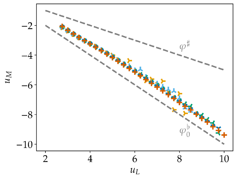
   (a) Standard choice of [78], $\varepsilon=10/N$.

   

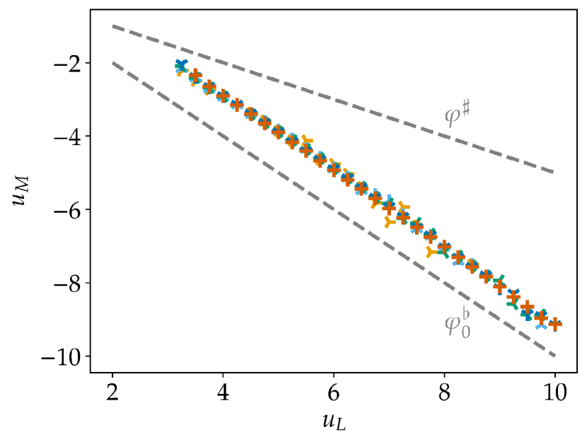
   (b) Convergent choice of [78], $\varepsilon=10/N$.

   Figure 18: Kinetic function for Fourier methods with different choices of the spectral viscosity and numbers $N$ of grid nodes.

3. The kinetic functions depend on the strength of the spectral viscosity. For the convergent choice of [78], nonclassical shocks can occur or not, depending on the strength $\varepsilon$. The strength $\varepsilon=100/N$ results in steeper kinetic function than the choice $\varepsilon=10/N$. For $\varepsilon=50/N$ and the convergent choice of [78], no nonclassical solutions appear, in contrast to the classical choice of the spectral viscosity which always results in nonclassical solutions. However, for smaller or bigger strengths of the spectral viscosity, nonclassical solutions occur even for the convergent choice of [78] and $N=$16\,384$$ grid nodes. This can be seen in Figure 19.

   

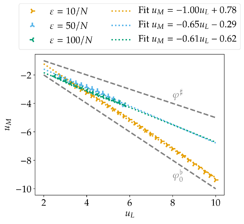
   (a) Standard choice of [78].

   

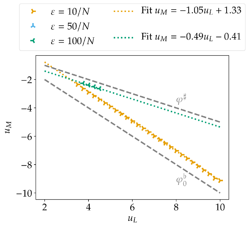
   (b) Convergent choice of [78].

   Figure 19: Kinetic function for Fourier methods with different choices of the spectral viscosity and $N=$16\,384$$ grid nodes.

4. In contrast to DG methods but similar to FD methods, the offset of the affine linear kinetic functions is in general not zero.

5. The kinetic functions satisfy the bounds (29).

5.5 WENO methods

In addition to the provably entropy-stable methods tested above, some standard shock capturing have been studied. Specifically, high-order WENO methods implemented in Clawpack [7, 49, 32, 31] have been investigated. The discretizations used WENO orders $p\in\{13,15,17\}$ and $N\in\{2^{8},2^{9},\dots,2^{14}\}$ cells with a CFL number of $0.5$. The other parameters of the problem are the same as for the SBP FD methods. The following observations have been made.

1. Nonclassical solutions have only been observed for very high-order WENO methods with $p\in\{13,15,17\}$. For $p\leq 11$, no nonclassical shocks occurred.

2. As for DG and FD methods, if the strength of the initial discontinuity is too big, no nonclassical solutions occurred and the critical strength of the initial discontinuity depends on the WENO order $p$.

3. The numerically obtained kinetic functions $\varphi^{\flat}$ are affine linear and seem to converge under grid refinement (or are already visually indistinguishable). This can be seen in Figure 20(a).

4. The kinetic functions do not seem to depend strongly on the WENO order $p$ when nonclassical solutions occur. For higher-order WENO methods, nonclassical shocks occurred also for bigger values of $u_{L}$. This can be seen in Figure 20(b).

   

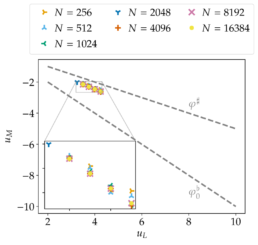
   (a) Grid refinement study for $p=17$.

   

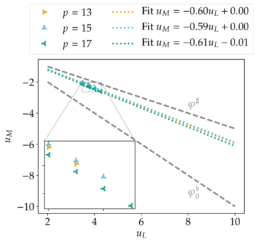
   (b) Different order $p$ for $N=$16\,384$$.

   Figure 20: Kinetic functions of WENO methods.

5. If few cells are used, the offset of the affine linear kinetic functions is not necessarily zero, similar to FD methods. For increased grid resolutions, the offset becomes (nearly) zero, similar to DG methods.

6. The kinetic functions satisfy the bounds (29).

6 Generalization to a quartic conservation law

6.1 Preliminaries

Entropy-conservative semi-discretizations of the scalar conservation law

$$\partial_{t}u(t,x)+\partial_{x}f(u(t,x)) =0,\quad t\in(0,T),\,x\in({x_{L}},{x_{R}}),$$ (30)

$$u(0,x) =u_{0}(x),\quad x\in({x_{L}},{x_{R}}),$$

$$f(u) =u^{2}(u^{2}-10)+3u,$$

can be constructed using the numerical flux

$$f^{\mathrm{num}}(u_{-},u_{+})=\frac{u_{+}^{4}+u_{-}u_{+}^{3}+u_{-}^{2}u_{+}^{2}+u_{-}^{3}u_{+}+u_{-}^{4}}{5}-10\frac{u_{+}^{2}+u_{-}u_{+}+u_{-}^{2}}{3}+3\frac{u_{+}+u_{-}}{2}$$ (31)

with corresponding split form

$$\frac{2}{5}\left(\underline{\underline{D}}\,\underline{u}^{4}+\underline{\underline{u}}\,\underline{\underline{D}}\,\underline{u}^{3}+\underline{\underline{u}}\,^{2}\underline{\underline{D}}\,\underline{u}^{2}+\underline{\underline{u}}\,^{3}\underline{\underline{D}}\,\underline{u}\right)-\frac{20}{3}\left(\underline{\underline{D}}\,\underline{u}^{2}+\underline{\underline{u}}\,\underline{\underline{D}}\,\underline{u}\right)+3\underline{\underline{D}}\,\underline{u},$$ (32)

cf. [57, Section 4.5]. The flux is visualized in Figure 21. To compute the kinetic function $\varphi^{\flat}$, Riemann problems with an initial condition

$$u_{0}(x)=\begin{cases}u_{R},&x\in[0,4.5],\\ u_{L},&\text{otherwise},\end{cases}$$ (33)

have been solved in the periodic domain $[-7,7]$ till the final time $t=3/\max\left\{\mathinner{\!\left\lvert f^{\prime}(u)\right\rvert}\;\middle|\;u_{L}\leq u\leq u_{R}\right\}$ for the fixed right state $u_{R}=2$.

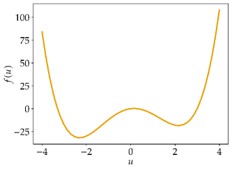
Figure 21: Non-convex flux function of the quartic conservation law (30).

Typical solutions obtained by a DG method are presented in Figure 22. For small left-hand states such as $u_{L}=-3.2$, the left-hand state is connected to classical wave. However, the right-hand state can be connected to a nonclassical state above $u_{R}$. For intermediate left-hand states such as $u_{L}=-2.0$, two nonclassical states occur, one below $u_{L}$ and one above $u_{R}$. For larger left-hand states such as $u_{L}=-1$, both the left and the right state are connected to a nonclassical state above $u_{R}$. In the following, the kinetic function $\varphi^{\flat}$ is computed as the mapping from a left-hand state $u_{L}$ to a nonclassical state below the left-hand state.

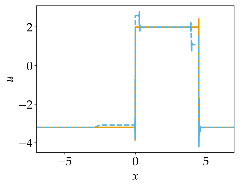
(a) $u_{L}=-3.2$.

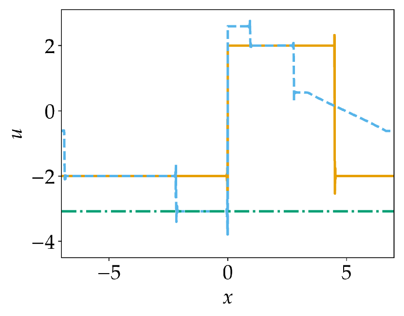
(b) $u_{L}=-2$.

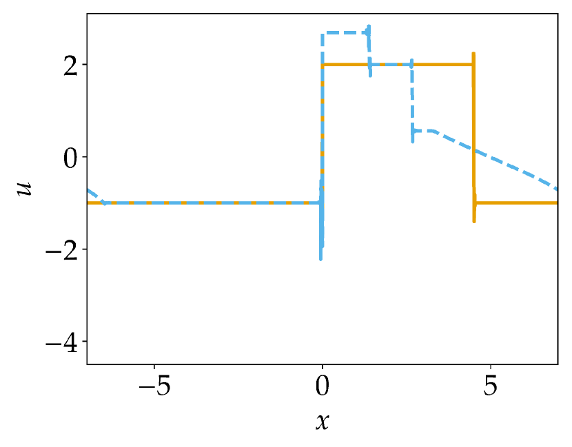
(c) $u_{L}=-1$.

Figure 22: Numerical solutions $u_{\mathrm{num}}$ (without postprocessing) of the Riemann problems with left-hand state $u_{L}$, right-hand state $u_{R}=2$, and a DG method with the following parameters: polynomial degree $p=5$, filter order $s=0$, number of elements $N=256$.

6.2 Nodal DG methods

For nodal DG methods, polynomial degrees $p\in\{0,1,\dots,5\}$, filter order $s\in\{0,1,\dots,5\}$, and numbers of elements $N\in\{2^{6},2^{7},\dots,2^{10}\}$ have been used. The numerical flux between elements is the entropy-dissipative flux obtained by adding local Lax-Friedrichs/Rusanov dissipation to the entropy conservative numerical flux (31). The following observations have been made.

1. The schemes with filter order $s\in\{1,2,3\}$ did not result in nonclassical solutions.

2. The finite volume schemes ($p=0$) did not result in nonclassical solutions. The schemes with polynomial degree $p\in\{1,2\}$ resulted in nonclassical solutions only if no filtering was applied ($s=0$).

3. For the investigated range of parameters, nonclassical solutions occurred only for $u_{L}\in[-4,-0.5]$ (as a necessary criterion). Depending on the other parameters, the extremal values of $u_{L}$ for which nonclassical solution occurred can be different.

4. The numerically obtained kinetic functions $\varphi^{\flat}$ are approximately constant. They remain visually indistinguishable under grid refinement by increasing the number of elements $N$. This is shown for $p=5$ and $s=5$ in Figure 23. The slight deviations from the constant value near the extremal values of $u_{L}$ are caused by oscillations of the numerical solutions.

   

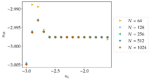
   Figure 23: Kinetic function for a DG method with polynomial degree $p=5$ and filter order $s=5$.

5. The kinetic functions do not depend on the polynomial degree $p$ if no filtering is applied, i.e. $s=0$. Otherwise, they depend on $p$. For $s=4$, $u_{M}$ is bigger for $p=4$ than for $p=5$ while it is the other way round for $s=5$. This is shown in Figure 24.

   

   

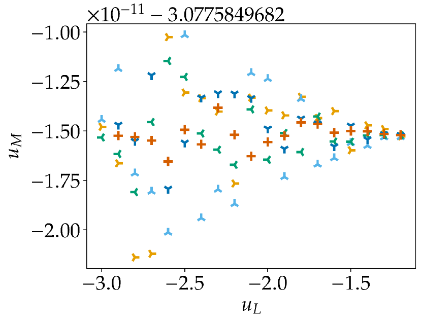
   (a) $s=0$.

   

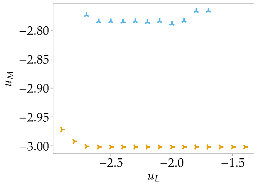
   (b) $s=4$.

   

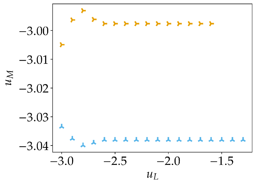
   (c) $s=5$.

   Figure 24: Kinetic function for DG methods with $N=$1024$$ elements.

6. The kinetic functions depend on the filter order $s$. However, there is no clear relation as shown in Figure 24.

6.3 Finite difference methods

For FD methods, accuracy order $p\in\{2,4,6\}$, artificial dissipation strength $\varepsilon_{i}\in\{0,100,\dots,400\}$, and $N\in\{2^{9},2^{10},\dots,2^{14}\}$ grid nodes have been used.

1. If artificial dissipation was applied, nonclassical solutions occurred at least for some values of $N$, even if only the second-order artificial dissipation was used ($\varepsilon_{2}\neq 0,\varepsilon_{4}=\varepsilon_{6}=0$). The only exception is given by the second-order method ($p=2$) with second-order artificial dissipation if $\varepsilon_{2}\neq 0$ is sufficiently big. This is again in agreement with [59].

2. As for DG methods, nonclassical solutions occured only for $u_{L}\in[-4,-0.5]$ for the investigated range of parameters.

3. The numerically obtained kinetic functions $\varphi^{\flat}$ are again approximately constant. They vary under grid refinement and the range of left-hand states $u_{L}$ for which nonclassical solutions with middle state $u_{M}<u_{L}$ occur typically increases with the number of grid points. This is shown in Figure 25.

   

   

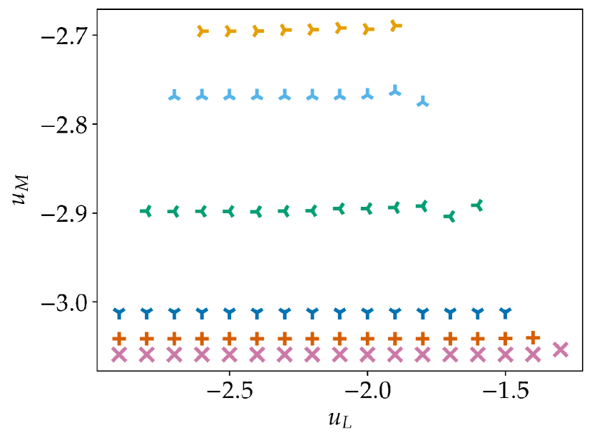
   (a) $\varepsilon_{2}=0$, $\varepsilon_{4}=100$, $\varepsilon_{6}=0$.

   

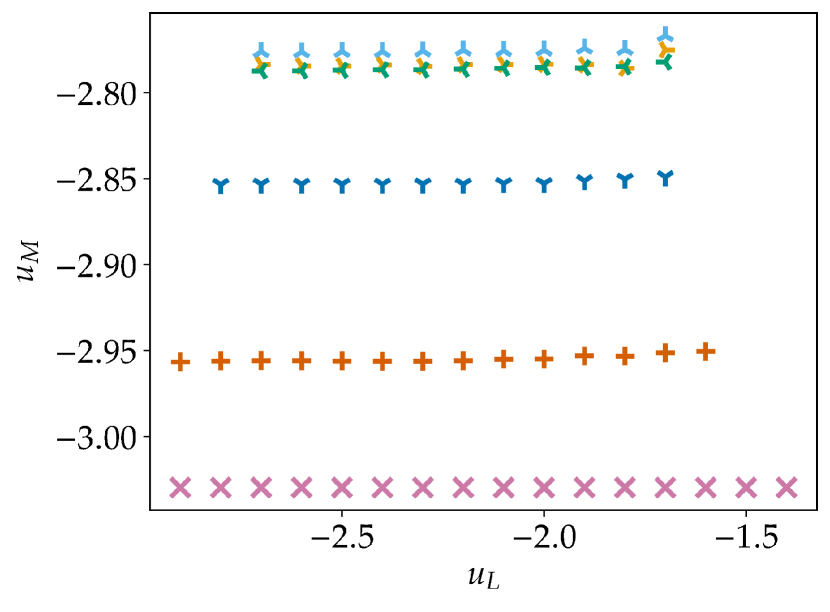
   (b) $\varepsilon_{2}=0$, $\varepsilon_{4}=0$, $\varepsilon_{6}=100$.

   Figure 25: Kinetic function for FD methods with order of accuracy $p=6$ and varying number of grid nodes $N$ for different orders of the artificial dissipation.

4. Choosing a fixed order of the artificial dissipation, i.e. $\varepsilon_{i}\in\{100,200,300,400\}$ and $\varepsilon_{j}=0$ for $j\neq i$, the kinetic functions depend on the strength $\varepsilon_{i}$. For high resolutions, the value of the kinetic function typically increases with the strength $\varepsilon_{i}$. This is shown in Figure 26.

   

   

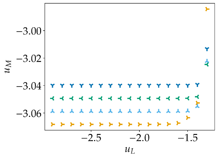
   (a) $\varepsilon_{2}=\varepsilon$, $\varepsilon_{4}=\varepsilon_{6}=0$.

   

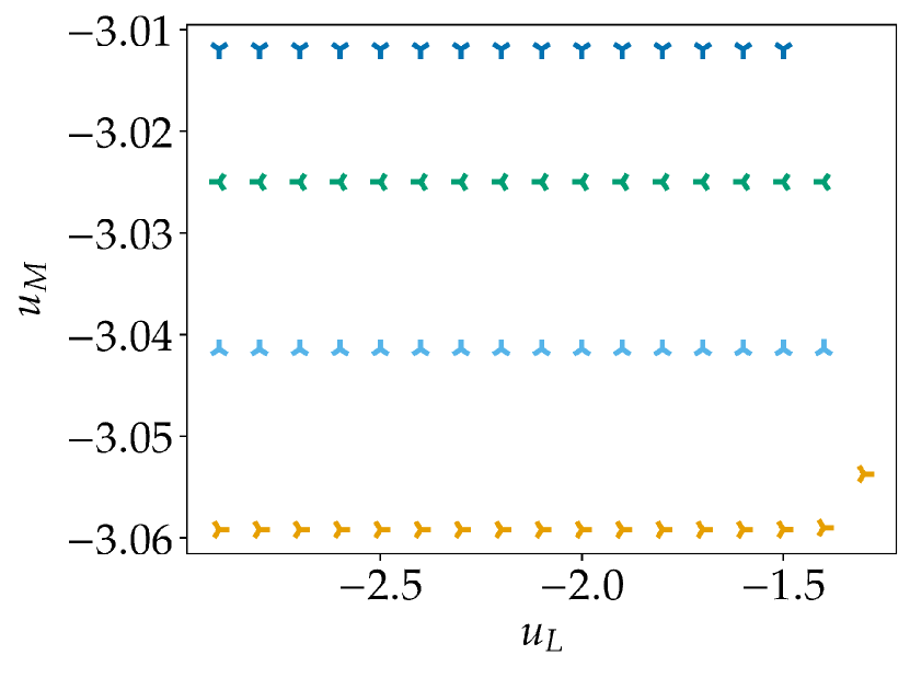
   (b) $\varepsilon_{4}=\varepsilon$, $\varepsilon_{2}=\varepsilon_{6}=0$.

   

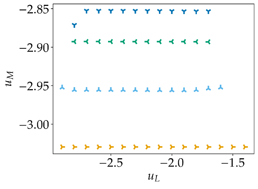
   (c) $\varepsilon_{6}=\varepsilon$, $\varepsilon_{2}=\varepsilon_{4}=0$.

   Figure 26: Kinetic function for FD methods with order of accuracy $p=6$, $N=$16\,384$$ grid nodes, and different strengths of the artificial dissipation.

5. The kinetic function varies slightly with the order of accuracy $p$. Typically, it increases (more negative) for higher values of $p$. This is shown in Figure 27.

   

   

   (a) $\varepsilon_{2}=0$, $\varepsilon_{4}=300$, $\varepsilon_{6}=0$.

   

   (b) $\varepsilon_{2}=0$, $\varepsilon_{4}=0$, $\varepsilon_{6}=400$.

   Figure 27: Kinetic function for FD methods with different orders of accuracy $p$, $N=$16\,384$$ grid nodes, and different strengths of the artificial dissipation.

6.4 Fourier collocation methods

For Fourier methods, the viscosity strengths $\varepsilon\in\{10/N,50/N,100/N\}$ for the standard and convergent choices of [78] and $N\in\{2^{10},2^{11},\dots,2^{14}\}$ grid nodes have been used. The following observations have been made.

1. As for DG and FD methods, nonclassical intermediate states $u_{M}<u_{L}$ occured only if $u_{L}\in[-4,-0.5]$ for the investigated range of parameters.

2. In contrast to DG and FD methods, not all numerically obtained kinetic functions $\varphi^{\flat}$ are approximately constant. If the strength of the standard spectral viscosity is low, there is a zig-zag behavior of the kinetic function that is stable under grid refinement. If the strength of the spectral viscosity is bigger, the kinetic functions are approximately constant and vary slightly under grid refinement, similarly to DG and FD methods. This is visualized in Figure 28.

   

   

   (a) $\varepsilon=10/N$.

   

   (b) $\varepsilon=100/N$.

   Figure 28: Kinetic function for Fourier methods using the standard choice of [78] with different strengths of the spectral viscosity and numbers $N$ of grid nodes.

3. The kinetic functions depend on the strength of the spectral viscosity. For the convergent choice of [78], nonclassical shocks can occur or not, depending on the strength $\varepsilon$. For example, many nonclassical shocks occured for $\varepsilon=10/N$, none for $\varepsilon=50/N$ and only a few for $\varepsilon=100/N$. In contrast, nonclassical solutions occured for all of these strengths if the classical spectral viscosity is applied. This can be seen in Figure 29.

   

   

   (a) Standard choice of [78].

   

   (b) Convergent choice of [78].

   Figure 29: Kinetic function for Fourier methods with different choices of the spectral viscosity and $N=$16\,384$$ grid nodes.

Remark 6.1.

Numerical experiments indicate that TeCNO methods based on the $L^{2}$ and $L^{4}$ entropy approximate the classical entropy solution for the setup considered here. However, it is unclear whether this is the case for all possible entropies and initial conditions.

7 Boundedness property for the Keyfitz-Kranzer system

7.1 Preliminaries

The Keyfitz-Kranzer system introduced in [34]

$$\partial_{t}u_{1}+\partial_{x}\bigl{(}u_{1}^{2}-u_{2}\bigr{)}=0,\qquad\partial_{t}u_{2}+\partial_{x}\bigl{(}\nicefrac{{u_{1}^{3}}}{{3}}-u_{1}\bigr{)}=0,$$ (34)

is strictly hyperbolic with eigenvalues $\lambda_{\pm}=u_{1}\pm 1$ and right eigenvectors $r_{\pm}=\big{(}1,u_{1}\mp 1\big{)}^{T}$. Thus, it is genuinely nonlinear. Moreover, it is straightforward to check that the convex function $U(u)=\exp\bigl{(}\nicefrac{{u_{1}^{2}}}{{2}}-u_{2}\bigr{)}$ is an entropy with associated entropy flux $F(u)=u_{1}U(u)$. Indeed, the entropy variables are

$$w(u)=U^{\prime}(u)=\begin{pmatrix}u_{1}U(u)\\ -U(u)\end{pmatrix}\quad\implies\quad U^{\prime\prime}(u)=\begin{pmatrix}1+u_{1}^{2}&-u_{1}\\ -u_{1}&1\end{pmatrix}U(u).$$ (35)

Thus, the flux potential is $\psi(u)=w(u)\cdot f(u)-F(u)=\left(\frac{2}{3}u_{1}^{3}-u_{1}u_{2}\right)\exp\bigl{(}\nicefrac{{u_{1}^{2}}}{{2}}-u_{2}\bigr{)}.$ Although there is a convex entropy and the system (34) is strictly hyperbolic and genuinely nonlinear, the Riemann problem can be solved in general only if measures are allowed in the solution [34]. These solutions are measures in space for fixed time. Especially, singular shock waves appear in the solution of certain Riemann problems, cf. [37, 33].

In order to construct entropy-stable semi-discretizations as entropy-conservative ones with additional dissipation, entropy-conservative numerical fluxes are sought. Using the procedure to derive entropy-conservative fluxes described in [56, Procedure 4.1], the following steps have to be performed:

1. Choose a set of variables, e.g. conservative variables, entropy variables, or something else.

2. Apply scalar differential mean values for $w$, $\psi$ to get an entropy conservative flux fulfilling $\raisebox{-2.5pt}{\leavevmode\resizebox{0.0pt}{7.5pt}{\raisebox{2.5pt}{$[\mkern-3.0mu[$}}}w\raisebox{-2.5pt}{\leavevmode\resizebox{0.0pt}{7.5pt}{\raisebox{2.5pt}{$]\mkern-3.0mu]$}}}\cdot f^{\mathrm{num}}=\raisebox{-2.5pt}{\leavevmode\resizebox{0.0pt}{8.3333pt}{\raisebox{2.5pt}{$[\mkern-3.0mu[$}}}\psi\raisebox{-2.5pt}{\leavevmode\resizebox{0.0pt}{8.3333pt}{\raisebox{2.5pt}{$]\mkern-3.0mu]$}}}$.

Due to the analytical form of the entropy variables $w$ (35) and the flux potential $\psi$ given earlier, the variables $u_{1}$ and $U(u)$ are used in the following. Of course, other choices are also possible. The jumps of the entropy variables can be written using the discrete product rule $\raisebox{-2.5pt}{\leavevmode\resizebox{0.0pt}{8.3333pt}{\raisebox{2.5pt}{$[\mkern-3.0mu[$}}}ab\raisebox{-2.5pt}{\leavevmode\resizebox{0.0pt}{8.3333pt}{\raisebox{2.5pt}{$]\mkern-3.0mu]$}}}=\raisebox{-2.5pt}{\leavevmode\resizebox{0.0pt}{7.5pt}{\raisebox{2.5pt}{$\{\mkern-6.0mu\{$}}}a\raisebox{-2.5pt}{\leavevmode\resizebox{0.0pt}{7.5pt}{\raisebox{2.5pt}{$\}\mkern-6.0mu\}$}}}\raisebox{-2.5pt}{\leavevmode\resizebox{0.0pt}{8.3333pt}{\raisebox{2.5pt}{$[\mkern-3.0mu[$}}}b\raisebox{-2.5pt}{\leavevmode\resizebox{0.0pt}{8.3333pt}{\raisebox{2.5pt}{$]\mkern-3.0mu]$}}}+\raisebox{-2.5pt}{\leavevmode\resizebox{0.0pt}{8.3333pt}{\raisebox{2.5pt}{$\{\mkern-6.0mu\{$}}}b\raisebox{-2.5pt}{\leavevmode\resizebox{0.0pt}{8.3333pt}{\raisebox{2.5pt}{$\}\mkern-6.0mu\}$}}}\raisebox{-2.5pt}{\leavevmode\resizebox{0.0pt}{7.5pt}{\raisebox{2.5pt}{$[\mkern-3.0mu[$}}}a\raisebox{-2.5pt}{\leavevmode\resizebox{0.0pt}{7.5pt}{\raisebox{2.5pt}{$]\mkern-3.0mu]$}}},$ with $\raisebox{-2.5pt}{\leavevmode\resizebox{0.0pt}{7.5pt}{\raisebox{2.5pt}{$[\mkern-3.0mu[$}}}a\raisebox{-2.5pt}{\leavevmode\resizebox{0.0pt}{7.5pt}{\raisebox{2.5pt}{$]\mkern-3.0mu]$}}}\mathrel{\mathop{\ordinarycolon}}=a_{+}-a_{-}$ and $\raisebox{-2.5pt}{\leavevmode\resizebox{0.0pt}{7.5pt}{\raisebox{2.5pt}{$\{\mkern-6.0mu\{$}}}a\raisebox{-2.5pt}{\leavevmode\resizebox{0.0pt}{7.5pt}{\raisebox{2.5pt}{$\}\mkern-6.0mu\}$}}}\mathrel{\mathop{\ordinarycolon}}=\frac{a_{+}+a_{-}}{2},$ as

$$\raisebox{-2.5pt}{\leavevmode\resizebox{0.0pt}{7.5pt}{\raisebox{2.5pt}{$[\mkern-3.0mu[$}}}w_{1}\raisebox{-2.5pt}{\leavevmode\resizebox{0.0pt}{7.5pt}{\raisebox{2.5pt}{$]\mkern-3.0mu]$}}}=\raisebox{-2.5pt}{\leavevmode\resizebox{0.0pt}{8.19995pt}{\raisebox{2.5pt}{$[\mkern-3.0mu[$}}}u_{1}U\raisebox{-2.5pt}{\leavevmode\resizebox{0.0pt}{8.19995pt}{\raisebox{2.5pt}{$]\mkern-3.0mu]$}}}=\raisebox{-2.5pt}{\leavevmode\resizebox{0.0pt}{7.5pt}{\raisebox{2.5pt}{$\{\mkern-6.0mu\{$}}}u_{1}\raisebox{-2.5pt}{\leavevmode\resizebox{0.0pt}{7.5pt}{\raisebox{2.5pt}{$\}\mkern-6.0mu\}$}}}\raisebox{-2.5pt}{\leavevmode\resizebox{0.0pt}{8.19995pt}{\raisebox{2.5pt}{$[\mkern-3.0mu[$}}}U\raisebox{-2.5pt}{\leavevmode\resizebox{0.0pt}{8.19995pt}{\raisebox{2.5pt}{$]\mkern-3.0mu]$}}}+\raisebox{-2.5pt}{\leavevmode\resizebox{0.0pt}{8.19995pt}{\raisebox{2.5pt}{$\{\mkern-6.0mu\{$}}}U\raisebox{-2.5pt}{\leavevmode\resizebox{0.0pt}{8.19995pt}{\raisebox{2.5pt}{$\}\mkern-6.0mu\}$}}}\raisebox{-2.5pt}{\leavevmode\resizebox{0.0pt}{7.5pt}{\raisebox{2.5pt}{$[\mkern-3.0mu[$}}}u_{1}\raisebox{-2.5pt}{\leavevmode\resizebox{0.0pt}{7.5pt}{\raisebox{2.5pt}{$]\mkern-3.0mu]$}}},\qquad\raisebox{-2.5pt}{\leavevmode\resizebox{0.0pt}{7.5pt}{\raisebox{2.5pt}{$[\mkern-3.0mu[$}}}w_{2}\raisebox{-2.5pt}{\leavevmode\resizebox{0.0pt}{7.5pt}{\raisebox{2.5pt}{$]\mkern-3.0mu]$}}}=-\raisebox{-2.5pt}{\leavevmode\resizebox{0.0pt}{8.19995pt}{\raisebox{2.5pt}{$[\mkern-3.0mu[$}}}U\raisebox{-2.5pt}{\leavevmode\resizebox{0.0pt}{8.19995pt}{\raisebox{2.5pt}{$]\mkern-3.0mu]$}}}.$$ (36)

Using the discrete chain rule

$$\raisebox{-2.5pt}{\leavevmode\resizebox{0.0pt}{8.3333pt}{\raisebox{2.5pt}{$[\mkern-3.0mu[$}}}\log a\raisebox{-2.5pt}{\leavevmode\resizebox{0.0pt}{8.3333pt}{\raisebox{2.5pt}{$]\mkern-3.0mu]$}}}=\frac{1}{\raisebox{-2.5pt}{\leavevmode\resizebox{0.0pt}{7.5pt}{\raisebox{2.5pt}{$\{\mkern-6.0mu\{$}}}a\raisebox{-2.5pt}{\leavevmode\resizebox{0.0pt}{7.5pt}{\raisebox{2.5pt}{$\}\mkern-6.0mu\}$}}}_{\mathrm{log}}}\raisebox{-2.5pt}{\leavevmode\resizebox{0.0pt}{7.5pt}{\raisebox{2.5pt}{$[\mkern-3.0mu[$}}}a\raisebox{-2.5pt}{\leavevmode\resizebox{0.0pt}{7.5pt}{\raisebox{2.5pt}{$]\mkern-3.0mu]$}}},\qquad\raisebox{-2.5pt}{\leavevmode\resizebox{0.0pt}{7.5pt}{\raisebox{2.5pt}{$\{\mkern-6.0mu\{$}}}a\raisebox{-2.5pt}{\leavevmode\resizebox{0.0pt}{7.5pt}{\raisebox{2.5pt}{$\}\mkern-6.0mu\}$}}}_{\mathrm{log}}\mathrel{\mathop{\ordinarycolon}}=\frac{\raisebox{-2.5pt}{\leavevmode\resizebox{0.0pt}{7.5pt}{\raisebox{2.5pt}{$[\mkern-3.0mu[$}}}a\raisebox{-2.5pt}{\leavevmode\resizebox{0.0pt}{7.5pt}{\raisebox{2.5pt}{$]\mkern-3.0mu]$}}}}{\raisebox{-2.5pt}{\leavevmode\resizebox{0.0pt}{8.3333pt}{\raisebox{2.5pt}{$[\mkern-3.0mu[$}}}\log a\raisebox{-2.5pt}{\leavevmode\resizebox{0.0pt}{8.3333pt}{\raisebox{2.5pt}{$]\mkern-3.0mu]$}}}},$$ (37)

for the logarithmic mean $\raisebox{-2.5pt}{\leavevmode\resizebox{0.0pt}{7.5pt}{\raisebox{2.5pt}{$\{\mkern-6.0mu\{$}}}a\raisebox{-2.5pt}{\leavevmode\resizebox{0.0pt}{7.5pt}{\raisebox{2.5pt}{$\}\mkern-6.0mu\}$}}}_{\mathrm{log}}$ [28] and $-u_{2}=\log(U)-\frac{1}{2}u_{1}^{2}$, the jump of the flux potential $\psi=\left(\frac{1}{6}u_{1}^{3}+u_{1}\log(U)\right)U$ can be written as

$$\raisebox{-2.5pt}{\leavevmode\resizebox{0.0pt}{8.3333pt}{\raisebox{2.5pt}{$[\mkern-3.0mu[$}}}\psi\raisebox{-2.5pt}{\leavevmode\resizebox{0.0pt}{8.3333pt}{\raisebox{2.5pt}{$]\mkern-3.0mu]$}}} =\raisebox{-3.86664pt}{\leavevmode\resizebox{0.0pt}{11.59995pt}{\raisebox{2.5pt}{$\{\mkern-6.0mu\{$}}}\frac{1}{6}u_{1}^{3}+u_{1}\log(U)\raisebox{-3.86664pt}{\leavevmode\resizebox{0.0pt}{11.59995pt}{\raisebox{2.5pt}{$\}\mkern-6.0mu\}$}}}\raisebox{-2.5pt}{\leavevmode\resizebox{0.0pt}{8.19995pt}{\raisebox{2.5pt}{$[\mkern-3.0mu[$}}}U\raisebox{-2.5pt}{\leavevmode\resizebox{0.0pt}{8.19995pt}{\raisebox{2.5pt}{$]\mkern-3.0mu]$}}}+\raisebox{-2.5pt}{\leavevmode\resizebox{0.0pt}{8.19995pt}{\raisebox{2.5pt}{$\{\mkern-6.0mu\{$}}}U\raisebox{-2.5pt}{\leavevmode\resizebox{0.0pt}{8.19995pt}{\raisebox{2.5pt}{$\}\mkern-6.0mu\}$}}}\raisebox{-3.86664pt}{\leavevmode\resizebox{0.0pt}{11.59995pt}{\raisebox{2.5pt}{$[\mkern-3.0mu[$}}}\frac{1}{6}u_{1}^{3}+u_{1}\log(U)\raisebox{-3.86664pt}{\leavevmode\resizebox{0.0pt}{11.59995pt}{\raisebox{2.5pt}{$]\mkern-3.0mu]$}}}$$ (38)

$$=\raisebox{-3.86664pt}{\leavevmode\resizebox{0.0pt}{11.59995pt}{\raisebox{2.5pt}{$\{\mkern-6.0mu\{$}}}\frac{1}{6}u_{1}^{3}+u_{1}\log(U)\raisebox{-3.86664pt}{\leavevmode\resizebox{0.0pt}{11.59995pt}{\raisebox{2.5pt}{$\}\mkern-6.0mu\}$}}}\raisebox{-2.5pt}{\leavevmode\resizebox{0.0pt}{8.19995pt}{\raisebox{2.5pt}{$[\mkern-3.0mu[$}}}U\raisebox{-2.5pt}{\leavevmode\resizebox{0.0pt}{8.19995pt}{\raisebox{2.5pt}{$]\mkern-3.0mu]$}}}+\frac{\raisebox{-2.5pt}{\leavevmode\resizebox{0.0pt}{8.19995pt}{\raisebox{2.5pt}{$\{\mkern-6.0mu\{$}}}U\raisebox{-2.5pt}{\leavevmode\resizebox{0.0pt}{8.19995pt}{\raisebox{2.5pt}{$\}\mkern-6.0mu\}$}}}}{\raisebox{-2.5pt}{\leavevmode\resizebox{0.0pt}{8.19995pt}{\raisebox{2.5pt}{$\{\mkern-6.0mu\{$}}}U\raisebox{-2.5pt}{\leavevmode\resizebox{0.0pt}{8.19995pt}{\raisebox{2.5pt}{$\}\mkern-6.0mu\}$}}}_{\mathrm{log}}}\raisebox{-2.5pt}{\leavevmode\resizebox{0.0pt}{7.5pt}{\raisebox{2.5pt}{$\{\mkern-6.0mu\{$}}}u_{1}\raisebox{-2.5pt}{\leavevmode\resizebox{0.0pt}{7.5pt}{\raisebox{2.5pt}{$\}\mkern-6.0mu\}$}}}\raisebox{-2.5pt}{\leavevmode\resizebox{0.0pt}{8.19995pt}{\raisebox{2.5pt}{$[\mkern-3.0mu[$}}}U\raisebox{-2.5pt}{\leavevmode\resizebox{0.0pt}{8.19995pt}{\raisebox{2.5pt}{$]\mkern-3.0mu]$}}}$$

$$\quad+\frac{1}{6}\raisebox{-2.5pt}{\leavevmode\resizebox{0.0pt}{8.19995pt}{\raisebox{2.5pt}{$\{\mkern-6.0mu\{$}}}U\raisebox{-2.5pt}{\leavevmode\resizebox{0.0pt}{8.19995pt}{\raisebox{2.5pt}{$\}\mkern-6.0mu\}$}}}\frac{\raisebox{-2.5pt}{\leavevmode\resizebox{0.0pt}{7.5pt}{\raisebox{2.5pt}{$[\mkern-3.0mu[$}}}u_{1}^{3}\raisebox{-2.5pt}{\leavevmode\resizebox{0.0pt}{7.5pt}{\raisebox{2.5pt}{$]\mkern-3.0mu]$}}}}{\raisebox{-2.5pt}{\leavevmode\resizebox{0.0pt}{7.5pt}{\raisebox{2.5pt}{$[\mkern-3.0mu[$}}}u_{1}\raisebox{-2.5pt}{\leavevmode\resizebox{0.0pt}{7.5pt}{\raisebox{2.5pt}{$]\mkern-3.0mu]$}}}}\raisebox{-2.5pt}{\leavevmode\resizebox{0.0pt}{7.5pt}{\raisebox{2.5pt}{$[\mkern-3.0mu[$}}}u_{1}\raisebox{-2.5pt}{\leavevmode\resizebox{0.0pt}{7.5pt}{\raisebox{2.5pt}{$]\mkern-3.0mu]$}}}+\raisebox{-2.5pt}{\leavevmode\resizebox{0.0pt}{8.19995pt}{\raisebox{2.5pt}{$\{\mkern-6.0mu\{$}}}U\raisebox{-2.5pt}{\leavevmode\resizebox{0.0pt}{8.19995pt}{\raisebox{2.5pt}{$\}\mkern-6.0mu\}$}}}\raisebox{-2.99998pt}{\leavevmode\resizebox{0.0pt}{8.99997pt}{\raisebox{2.5pt}{$\{\mkern-6.0mu\{$}}}\log(U)\raisebox{-2.99998pt}{\leavevmode\resizebox{0.0pt}{8.99997pt}{\raisebox{2.5pt}{$\}\mkern-6.0mu\}$}}}\raisebox{-2.5pt}{\leavevmode\resizebox{0.0pt}{7.5pt}{\raisebox{2.5pt}{$[\mkern-3.0mu[$}}}u_{1}\raisebox{-2.5pt}{\leavevmode\resizebox{0.0pt}{7.5pt}{\raisebox{2.5pt}{$]\mkern-3.0mu]$}}}.$$

Here, we have $\frac{\raisebox{-1.75pt}{\leavevmode\resizebox{0.0pt}{5.25pt}{\raisebox{1.75pt}{$[\mkern-3.0mu[$}}}a^{3}\raisebox{-1.75pt}{\leavevmode\resizebox{0.0pt}{5.25pt}{\raisebox{1.75pt}{$]\mkern-3.0mu]$}}}}{\raisebox{-1.75pt}{\leavevmode\resizebox{0.0pt}{5.25pt}{\raisebox{1.75pt}{$[\mkern-3.0mu[$}}}a\raisebox{-1.75pt}{\leavevmode\resizebox{0.0pt}{5.25pt}{\raisebox{1.75pt}{$]\mkern-3.0mu]$}}}}=\frac{a_{+}^{3}-a_{-}^{3}}{a_{+}-a_{-}}=a_{+}^{2}+a_{+}a_{-}+a_{-}^{2}.$ Therefore, the condition $\raisebox{-2.5pt}{\leavevmode\resizebox{0.0pt}{7.5pt}{\raisebox{2.5pt}{$[\mkern-3.0mu[$}}}w\raisebox{-2.5pt}{\leavevmode\resizebox{0.0pt}{7.5pt}{\raisebox{2.5pt}{$]\mkern-3.0mu]$}}}\cdot f^{\mathrm{num}}-\raisebox{-2.5pt}{\leavevmode\resizebox{0.0pt}{8.3333pt}{\raisebox{2.5pt}{$[\mkern-3.0mu[$}}}\psi\raisebox{-2.5pt}{\leavevmode\resizebox{0.0pt}{8.3333pt}{\raisebox{2.5pt}{$]\mkern-3.0mu]$}}}=0$ (11) for an entropy-conservative flux becomes

$$0=\left(\raisebox{-2.5pt}{\leavevmode\resizebox{0.0pt}{7.5pt}{\raisebox{2.5pt}{$\{\mkern-6.0mu\{$}}}u_{1}\raisebox{-2.5pt}{\leavevmode\resizebox{0.0pt}{7.5pt}{\raisebox{2.5pt}{$\}\mkern-6.0mu\}$}}}f^{\mathrm{num}}_{1}-f^{\mathrm{num}}_{2}-\raisebox{-3.86664pt}{\leavevmode\resizebox{0.0pt}{11.59995pt}{\raisebox{2.5pt}{$\{\mkern-6.0mu\{$}}}\frac{1}{6}u_{1}^{3}+u_{1}\log(U)\raisebox{-3.86664pt}{\leavevmode\resizebox{0.0pt}{11.59995pt}{\raisebox{2.5pt}{$\}\mkern-6.0mu\}$}}}-\frac{\raisebox{-2.5pt}{\leavevmode\resizebox{0.0pt}{8.19995pt}{\raisebox{2.5pt}{$\{\mkern-6.0mu\{$}}}U\raisebox{-2.5pt}{\leavevmode\resizebox{0.0pt}{8.19995pt}{\raisebox{2.5pt}{$\}\mkern-6.0mu\}$}}}}{\raisebox{-2.5pt}{\leavevmode\resizebox{0.0pt}{8.19995pt}{\raisebox{2.5pt}{$\{\mkern-6.0mu\{$}}}U\raisebox{-2.5pt}{\leavevmode\resizebox{0.0pt}{8.19995pt}{\raisebox{2.5pt}{$\}\mkern-6.0mu\}$}}}_{\mathrm{log}}}\raisebox{-2.5pt}{\leavevmode\resizebox{0.0pt}{7.5pt}{\raisebox{2.5pt}{$\{\mkern-6.0mu\{$}}}u_{1}\raisebox{-2.5pt}{\leavevmode\resizebox{0.0pt}{7.5pt}{\raisebox{2.5pt}{$\}\mkern-6.0mu\}$}}}\right)\raisebox{-2.5pt}{\leavevmode\resizebox{0.0pt}{8.19995pt}{\raisebox{2.5pt}{$[\mkern-3.0mu[$}}}U\raisebox{-2.5pt}{\leavevmode\resizebox{0.0pt}{8.19995pt}{\raisebox{2.5pt}{$]\mkern-3.0mu]$}}}\\ +\left(\raisebox{-2.5pt}{\leavevmode\resizebox{0.0pt}{8.19995pt}{\raisebox{2.5pt}{$\{\mkern-6.0mu\{$}}}U\raisebox{-2.5pt}{\leavevmode\resizebox{0.0pt}{8.19995pt}{\raisebox{2.5pt}{$\}\mkern-6.0mu\}$}}}f^{\mathrm{num}}_{1}-\frac{1}{6}\raisebox{-2.5pt}{\leavevmode\resizebox{0.0pt}{8.19995pt}{\raisebox{2.5pt}{$\{\mkern-6.0mu\{$}}}U\raisebox{-2.5pt}{\leavevmode\resizebox{0.0pt}{8.19995pt}{\raisebox{2.5pt}{$\}\mkern-6.0mu\}$}}}\frac{\raisebox{-2.5pt}{\leavevmode\resizebox{0.0pt}{7.5pt}{\raisebox{2.5pt}{$[\mkern-3.0mu[$}}}u_{1}^{3}\raisebox{-2.5pt}{\leavevmode\resizebox{0.0pt}{7.5pt}{\raisebox{2.5pt}{$]\mkern-3.0mu]$}}}}{\raisebox{-2.5pt}{\leavevmode\resizebox{0.0pt}{7.5pt}{\raisebox{2.5pt}{$[\mkern-3.0mu[$}}}u_{1}\raisebox{-2.5pt}{\leavevmode\resizebox{0.0pt}{7.5pt}{\raisebox{2.5pt}{$]\mkern-3.0mu]$}}}}-\raisebox{-2.5pt}{\leavevmode\resizebox{0.0pt}{8.19995pt}{\raisebox{2.5pt}{$\{\mkern-6.0mu\{$}}}U\raisebox{-2.5pt}{\leavevmode\resizebox{0.0pt}{8.19995pt}{\raisebox{2.5pt}{$\}\mkern-6.0mu\}$}}}\raisebox{-2.99998pt}{\leavevmode\resizebox{0.0pt}{8.99997pt}{\raisebox{2.5pt}{$\{\mkern-6.0mu\{$}}}\log(U)\raisebox{-2.99998pt}{\leavevmode\resizebox{0.0pt}{8.99997pt}{\raisebox{2.5pt}{$\}\mkern-6.0mu\}$}}}\right)\raisebox{-2.5pt}{\leavevmode\resizebox{0.0pt}{7.5pt}{\raisebox{2.5pt}{$[\mkern-3.0mu[$}}}u_{1}\raisebox{-2.5pt}{\leavevmode\resizebox{0.0pt}{7.5pt}{\raisebox{2.5pt}{$]\mkern-3.0mu]$}}}.$$ (39)

Hence,

$$f^{\mathrm{num}}_{1} =\frac{1}{6}\frac{\raisebox{-2.5pt}{\leavevmode\resizebox{0.0pt}{7.5pt}{\raisebox{2.5pt}{$[\mkern-3.0mu[$}}}u_{1}^{3}\raisebox{-2.5pt}{\leavevmode\resizebox{0.0pt}{7.5pt}{\raisebox{2.5pt}{$]\mkern-3.0mu]$}}}}{\raisebox{-2.5pt}{\leavevmode\resizebox{0.0pt}{7.5pt}{\raisebox{2.5pt}{$[\mkern-3.0mu[$}}}u_{1}\raisebox{-2.5pt}{\leavevmode\resizebox{0.0pt}{7.5pt}{\raisebox{2.5pt}{$]\mkern-3.0mu]$}}}}+\raisebox{-2.99998pt}{\leavevmode\resizebox{0.0pt}{8.99997pt}{\raisebox{2.5pt}{$\{\mkern-6.0mu\{$}}}\log(U)\raisebox{-2.99998pt}{\leavevmode\resizebox{0.0pt}{8.99997pt}{\raisebox{2.5pt}{$\}\mkern-6.0mu\}$}}},$$ (40)

$$f^{\mathrm{num}}_{2} =\raisebox{-2.5pt}{\leavevmode\resizebox{0.0pt}{7.5pt}{\raisebox{2.5pt}{$\{\mkern-6.0mu\{$}}}u_{1}\raisebox{-2.5pt}{\leavevmode\resizebox{0.0pt}{7.5pt}{\raisebox{2.5pt}{$\}\mkern-6.0mu\}$}}}f^{\mathrm{num}}_{1}-\raisebox{-3.86664pt}{\leavevmode\resizebox{0.0pt}{11.59995pt}{\raisebox{2.5pt}{$\{\mkern-6.0mu\{$}}}\frac{1}{6}u_{1}^{3}+u_{1}\log(U)\raisebox{-3.86664pt}{\leavevmode\resizebox{0.0pt}{11.59995pt}{\raisebox{2.5pt}{$\}\mkern-6.0mu\}$}}}-\frac{\raisebox{-2.5pt}{\leavevmode\resizebox{0.0pt}{8.19995pt}{\raisebox{2.5pt}{$\{\mkern-6.0mu\{$}}}U\raisebox{-2.5pt}{\leavevmode\resizebox{0.0pt}{8.19995pt}{\raisebox{2.5pt}{$\}\mkern-6.0mu\}$}}}}{\raisebox{-2.5pt}{\leavevmode\resizebox{0.0pt}{8.19995pt}{\raisebox{2.5pt}{$\{\mkern-6.0mu\{$}}}U\raisebox{-2.5pt}{\leavevmode\resizebox{0.0pt}{8.19995pt}{\raisebox{2.5pt}{$\}\mkern-6.0mu\}$}}}_{\mathrm{log}}}\raisebox{-2.5pt}{\leavevmode\resizebox{0.0pt}{7.5pt}{\raisebox{2.5pt}{$\{\mkern-6.0mu\{$}}}u_{1}\raisebox{-2.5pt}{\leavevmode\resizebox{0.0pt}{7.5pt}{\raisebox{2.5pt}{$\}\mkern-6.0mu\}$}}},$$

can be seen to yield an entropy-conservative numerical flux for the Keyfitz-Kranzer system (34) with the entropy $U(u)=\exp(\nicefrac{{u_{1}^{2}}}{{2}}-u_{2})$. In order to create an entropy-stable numerical flux, the local Lax-Friedrichs/Rusanov type dissipation $-\frac{\lambda}{2}\raisebox{-2.5pt}{\leavevmode\resizebox{0.0pt}{7.5pt}{\raisebox{2.5pt}{$[\mkern-3.0mu[$}}}u\raisebox{-2.5pt}{\leavevmode\resizebox{0.0pt}{7.5pt}{\raisebox{2.5pt}{$]\mkern-3.0mu]$}}}$ will be added to the numerical flux (40), where $\lambda=\max\left\{\mathinner{\!\left\lvert u_{1,-}\right\rvert},\mathinner{\!\left\lvert u_{1,+}\right\rvert}\right\}+1$ is the maximal eigenvalue of both arguments $u_{\pm}$.

In the following, the Riemann problem at $x=0$ with left and right initial data

$$u_{L}=\begin{pmatrix}1.5\\ 0\end{pmatrix},\qquad u_{R}=\begin{pmatrix}-2.065426\\ 1.410639\end{pmatrix},$$ (41)

given in [70, Section 4] will be considered in the domain $({x_{L}},{x_{R}})=(-3/4,1/4)$ up to the final time $T=2$. Since the solution does not interact with the boundary during this time, constant boundary values are assumed. The continuous rate of change of the entropy is $\dfrac{\operatorname{d\!}{}}{\operatorname{d\!}{t}}\int_{x_{L}}^{x_{R}}U=-F\big{|}_{x_{L}}^{x_{R}}=F(g_{L})-F(g_{R}),$ if the left and right boundary data are $g_{L},g_{R}$. Thus, the entropy rate is bounded by data if $F_{L}\geq 0$ and $F_{R}\leq 0$, which is fulfilled for the given Riemann problem, since $F(u)=u_{1}\exp(u_{1}^{2}/2-u_{2})$ and $u_{1}>0$ on the left-hand side and $u_{1}<0$ on the right-hand side. The semi-discrete entropy rate is

$$\underline{w}^{T}\underline{\underline{M}}\,\partial_{t}\underline{u}=\left(w_{L}\cdot f^{\mathrm{num}}_{L}-\psi_{L}\right)-\left(w_{R}\cdot f^{\mathrm{num}}_{R}-\psi_{R}\right).$$ (42)

In order to bound the semi-discrete entropy rate by the continuous one, only the left-hand side is considered in the following. The other side can be handled similarly. Here, the condition

$$\left(w_{L}\cdot f^{\mathrm{num}}_{L}-\psi_{L}\right)\leq F(g_{L})=w(g_{L})\cdot f(g_{L})-\psi(g_{L})$$ (43)

is required for the semi-discretization. If the numerical flux $f^{\mathrm{num}}$ is entropy stable, $\bigl{(}w_{L}-w(g_{L})\bigr{)}\cdot f^{\mathrm{num}}_{L}-\bigl{(}\psi_{L}-\psi(g_{L})\bigr{)}\leq 0$. Thus, (43) is fulfilled if $w(g_{L})\cdot f^{\mathrm{num}}_{L}-\psi(g_{L})\leq w(g_{L})\cdot f(g_{L})-\psi(g_{L}),$ which is equivalent to

$$w(g_{L})\cdot\left(f^{\mathrm{num}}(g_{L},u_{L})-f(g_{L})\right)\leq 0.$$ (44)

It seems to be technically difficult to check this condition for the entropy stable flux using the local Lax-Friedrichs-Rusanov type dissipation. However, it can be checked during the numerical experiments. There, it is fulfilled up to machine accuracy in the Riemann problems under consideration.

7.2 Numerical results

First-order finite volume discretizations based on the entropy-stable flux above are now applied. An explicit Euler method is used in order to advance the numerical solution in time, up to $T=2$, and the time step is chosen adaptively as $\Delta t=\frac{\Delta x}{2\lambda}$, where $\lambda=\max\left\{\mathinner{\!\left\lvert u_{i,1}\right\rvert}+1\right\}$ is the maximal advection speed of the numerical solution. A typical solution at $t=T$ is displayed in Figure 30. A singular shock occurs and moves to the left, cf. [70, Section 4]. The maximal values of each component increase with increasing resolution, since the analytical solution contains a Dirac mass moving with the shock. This behavior is visualized in Figure 31. The maximal values of the numerical solutions increase over time, in agreement with the increasing mass of the delta measure. Clearly, in general, entropy stability does not imply boundedness of numerical solutions.

(a) First component $u_{1}$.

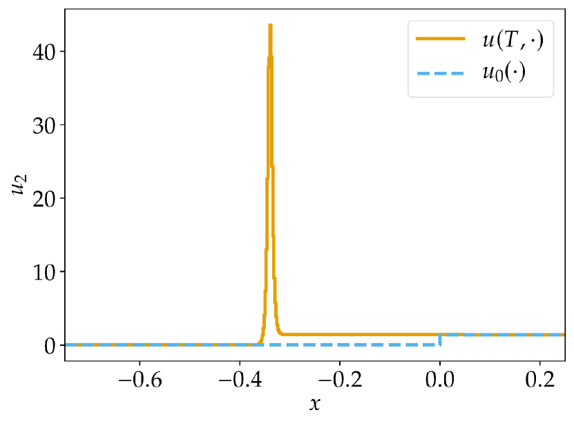
(b) Second component $u_{2}$.

Figure 30: Numerical solutions using the first order finite volume method with $N=512$ cells at the final time $t=T$.

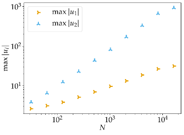
Figure 31: Extreme values of the numerical solutions using the first order finite volume method with $N$ cells at the final time $t=T$.

8 Summary and conclusions

We studied a variety of entropy-dissipative numerical methods for nonlinear scalar conservation laws with non-convex flux in one space dimension, including finite difference methods with artificial dissipation, discontinuous Galerkin methods with or without filtering, and Fourier methods with (super-) spectral viscosity. We demonstrated experimentally that all these numerical methods can converge to different weak solutions, either the classical entropy solution or weak solutions involving nonclassical shock waves. For the same class of methods, the convergence depends also on associated parameters; changing a parameter such as the order or strength of dissipation changes the limiting solution in general. Moreover, we demonstrated that numerical solutions can also depend on the specific choice of the entropy function, e.g. for TeCNO schemes. To distinguish the different convergence behavior of the numerical methods, we also computed the associated kinetic functions for a variety of schemes, including also high-order WENO methods. Finally, we developed entropy-dissipative numerical methods for the Keyfitz-Kranzer system, demonstrating that entropy-dissipative methods may generate numerical solutions that do not remain bounded under grid refinement.

Our results provide important contributions to the theory of nonclassical shocks by comparing a variety of numerical schemes and their kinetic functions. On the other hand, these results also demonstrate limitations of modern high-order entropy-dissipative methods, complementing the recent investigations [20, 62]. Hence, we stress the importance of choosing appropriate regularizations to compute numerical solutions of conservation laws, in particular if they support nonclassical shock waves as weak solutions.

References

- [1] Christophe Berthon, Frédéric Coquel and Philippe G. LeFloch “Why many theories of shock waves are necessary: kinetic relations for non-conservative systems” In Proc. Roy. Soc. Edinburgh Sect. A 142.1, 2012, pp. 1–37 DOI: 10.1017/S0308210510001009
- [2] Jeff Bezanson, Alan Edelman, Stefan Karpinski and Viral B Shah “Julia: A Fresh Approach to Numerical Computing” In SIAM Review 59.1 SIAM, 2017, pp. 65–98 DOI: 10.1137/141000671
- [3] Mark H Carpenter, David Gottlieb and Saul Abarbanel “Time-Stable Boundary Conditions for Finite-Difference Schemes Solving Hyperbolic Systems: Methodology and Application to High-Order Compact Schemes” In Journal of Computational Physics 111.2 Elsevier, 1994, pp. 220–236 DOI: 10.1006/jcph.1994.1057
- [4] Mark H Carpenter, Jan Nordström and David Gottlieb “A Stable and Conservative Interface Treatment of Arbitrary Spatial Accuracy” In Journal of Computational Physics 148.2 Elsevier, 1999, pp. 341–365 DOI: 10.1006/jcph.1998.6114
- [5] Manuel J Castro, Philippe G LeFloch, María Luz Muñoz-Ruiz and Carlos Parés “Why many theories of shock waves are necessary: Convergence error in formally path-consistent schemes” In Journal of Computational Physics 227.17 Elsevier, 2008, pp. 8107–8129 DOI: 10.1016/j.jcp.2008.05.012
- [6] Tianheng Chen and Chi-Wang Shu “Entropy stable high order discontinuous Galerkin methods with suitable quadrature rules for hyperbolic conservation laws” In Journal of Computational Physics 345 Elsevier, 2017, pp. 427–461 DOI: 10.1016/j.jcp.2017.05.025
- [7] Clawpack Development Team “Clawpack software” Version 5.6.1, 2019 DOI: 10.5281/zenodo.3528429
- [8] Laurent Condat “A direct algorithm for 1-D total variation denoising” In IEEE Signal Processing Letters 20.11 IEEE, 2013, pp. 1054–1057 DOI: 10.1109/LSP.2013.2278339
- [9] Constantine M Dafermos “The entropy rate admissibility criterion for solutions of hyperbolic conservation laws” In Journal of Differential Equations 14.2 Elsevier, 1973, pp. 202–212 DOI: 10.1016/0022-0396(73)90043-0
- [10] Camillo De Lellis, Felix Otto and Michael Westdickenberg “Minimal entropy conditions for Burgers equation” In Quarterly of Applied Mathematics 62.4 American Mathematical Society, 2004, pp. 687–700 DOI: 10.1090/qam/2104269
- [11] David C Del Rey Fernández, Pieter D Boom and David W Zingg “A generalized framework for nodal first derivative summation-by-parts operators” In Journal of Computational Physics 266 Elsevier, 2014, pp. 214–239 DOI: 10.1016/j.jcp.2014.01.038
- [12] David C Del Rey Fernández, Jason E Hicken and David W Zingg “Review of summation-by-parts operators with simultaneous approximation terms for the numerical solution of partial differential equations” In Computers & Fluids 95 Elsevier, 2014, pp. 171–196 DOI: 10.1016/j.compfluid.2014.02.016
- [13] Travis C Fisher and Mark H Carpenter “High-order entropy stable finite difference schemes for nonlinear conservation laws: Finite domains” In Journal of Computational Physics 252 Elsevier, 2013, pp. 518–557 DOI: 10.1016/j.jcp.2013.06.014
- [14] Ulrik Skre Fjordholm “High-order accurate entropy stable numerical schemes for hyperbolic conservation laws”, 2013 DOI: 10.3929/ethz-a-007622508
- [15] Ulrik Skre Fjordholm, Roger Käppeli, Siddhartha Mishra and Eitan Tadmor “Construction of Approximate Entropy Measure-Valued Solutions for Hyperbolic Systems of Conservation Laws” In Foundations of Computational Mathematics 17 Springer, 2017, pp. 763–827 DOI: 10.1007/s10208-015-9299-z
- [16] Ulrik Skre Fjordholm, Siddhartha Mishra and Eitan Tadmor “Arbitrarily High-Order Accurate Entropy Stable Essentially Nonoscillatory Schemes for Systems of Conservation Laws” In SIAM Journal on Numerical Analysis 50.2 Society for IndustrialApplied Mathematics, 2012, pp. 544–573 DOI: 10.1137/110836961
- [17] Ulrik Skre Fjordholm, Siddhartha Mishra and Eitan Tadmor “ENO Reconstruction and ENO Interpolation Are Stable” In Foundations of Computational Mathematics 13.2 Springer, 2013, pp. 139–159 DOI: 10.1007/s10208-012-9117-9
- [18] Ulrik Skre Fjordholm, Siddhartha Mishra and Eitan Tadmor “On the computation of measure-valued solutions” In Acta Numerica 25 Cambridge Univ Press, 2016, pp. 567–679 DOI: 10.1017/S0962492916000088
- [19] Gregor J Gassner “A Skew-Symmetric Discontinuous Galerkin Spectral Element Discretization and Its Relation to SBP-SAT Finite Difference Methods” In SIAM Journal on Scientific Computing 35.3 Society for IndustrialApplied Mathematics, 2013, pp. A1233–A1253 DOI: 10.1137/120890144
- [20] Gregor J Gassner, Magnus Svärd and Florian J Hindenlang “Stability issues of entropy-stable and/or split-form high-order schemes”, 2020 arXiv:2007.09026 [math.NA]
- [21] Ben-Yu Guo, He-Ping Ma and Eitan Tadmor “Spectral vanishing viscosity method for nonlinear conservation laws” In SIAM Journal on Numerical Analysis 39.4 SIAM, 2001, pp. 1254–1268
- [22] Brian T Hayes and Philippe G LeFloch “Non-classical shocks and kinetic relations: Scalar conservation laws” In Archive for Rational Mechanics and Analysis 139.1 Springer, 1997, pp. 1–56 DOI: 10.1007/s002050050046
- [23] Brian T Hayes and Philippe G LeFloch “Nonclassical shocks and kinetic relations: Finite difference schemes” In SIAM journal on numerical analysis 35.6 SIAM, 1998, pp. 2169–2194 DOI: 10.1137/S0036142997315998
- [24] Jan Hesthaven and Robert Kirby “Filtering in Legendre spectral methods” In Mathematics of Computation 77.263 American Mathematical Society, 2008, pp. 1425–1452 DOI: 10.1090/S0025-5718-08-02110-8
- [25] Jason E Hicken “Entropy-stable, high-order summation-by-parts discretizations without interface penalties” In Journal of Scientific Computing 82.2 Springer, 2020, pp. 50 DOI: 10.1007/s10915-020-01154-8
- [26] Jason E Hicken, David C Del Rey Fernández and David W Zingg “Multidimensional Summation-By-Parts Operators: General Theory and Application to Simplex Elements” In SIAM Journal on Scientific Computing 38.4 Society for IndustrialApplied Mathematics, 2016, pp. A1935–A1958 DOI: 10.1137/15M1038360
- [27] Thomas Y Hou and Philippe G LeFloch “Why nonconservative schemes converge to wrong solutions: Error analysis” In Mathematics of Computation 62.206 American Mathematical Society, 1994, pp. 497–530 DOI: 10.1090/S0025-5718-1994-1201068-0
- [28] Farzad Ismail and Philip L Roe “Affordable, entropy-consistent Euler flux functions II: Entropy production at shocks” In Journal of Computational Physics 228.15 Elsevier, 2009, pp. 5410–5436 DOI: 10.1016/j.jcp.2009.04.021
- [29] David I Ketcheson “Highly Efficient Strong Stability-Preserving Runge-Kutta Methods with Low-Storage Implementations” In SIAM Journal on Scientific Computing 30.4 Society for IndustrialApplied Mathematics, 2008, pp. 2113–2136 DOI: 10.1137/07070485X
- [30] David I Ketcheson “Relaxation Runge-Kutta Methods: Conservation and Stability for Inner-Product Norms” In SIAM Journal on Numerical Analysis 57.6 Society for IndustrialApplied Mathematics, 2019, pp. 2850–2870 DOI: 10.1137/19M1263662
- [31] David I Ketcheson et al. “PyClaw: Accessible, extensible, scalable tools for wave propagation problems” In SIAM Journal on Scientific Computing 34.4 SIAM, 2012, pp. C210–C231 DOI: 10.1137/110856976
- [32] David I Ketcheson, Matteo Parsani and Randall J LeVeque “High-order wave propagation algorithms for hyperbolic systems” In SIAM Journal on Scientific Computing 35.1 SIAM, 2013, pp. A351–A377 DOI: 10.1137/110830320
- [33] Barbara Lee Keyfitz “Singular shocks: retrospective and prospective” In Confluentes Mathematici 3.03 World Scientific, 2011, pp. 445–470 DOI: 10.1142/S1793744211000424
- [34] Barbara Lee Keyfitz and Herbert C Kranzer “Spaces of weighted measures for conservation laws with singular shock solutions” In Journal of Differential Equations 118.2 Elsevier, 1995, pp. 420–451 DOI: 10.1006/jdeq.1995.1080
- [35] David A Kopriva and Gregor J Gassner “On the Quadrature and Weak Form Choices in Collocation Type Discontinuous Galerkin Spectral Element Methods” In Journal of Scientific Computing 44.2 Springer, 2010, pp. 136–155 DOI: 10.1007/s10915-010-9372-3
- [36] Heinz-Otto Kreiss and Godela Scherer “Finite Element and Finite Difference Methods for Hyperbolic Partial Differential Equations” In Mathematical Aspects of Finite Elements in Partial Differential Equations New York: Academic Press, 1974, pp. 195–212
- [37] Philippe G LeFloch “An existence and uniqueness result for two nonstrictly hyperbolic systems” In Nonlinear evolution equations that change type 27, IMA Vol. Math. Appl. Springer, New York, 1990, pp. 126–138 DOI: 10.1007/978-1-4613-9049-7_10
- [38] Philippe G LeFloch “An introduction to nonclassical shocks of systems of conservation laws” In An introduction to recent developments in theory and numerics for conservation laws 5, Lecture Notes in Computational Science and Engineering Berlin, Heidelberg: Springer, 1999, pp. 28–72 DOI: 10.1007/978-3-642-58535-7_2
- [39] Philippe G LeFloch “Hyperbolic Systems of Conservation Laws: The Theory of Classical and Nonclassical Shock Waves” Basel: Birkhäuser, 2002 DOI: 10.1007/978-3-0348-8150-0
- [40] Philippe G LeFloch “Kinetic relations for undercompressive shock waves. Physical, mathematical, and numerical issues” In Nonlinear Partial Differential Equations and Hyperbolic Wave Phenomena 526, Contemporary Mathematics Providence, RI: American Mathematical Society, 2010, pp. 237–272
- [41] Philippe G LeFloch, Jean-Marc Mercier and Christian Rohde “Fully Discrete, Entropy Conservative Schemes of Arbitrary Order” In SIAM Journal on Numerical Analysis 40.5 Society for IndustrialApplied Mathematics, 2002, pp. 1968–1992 DOI: 10.1137/S003614290240069X
- [42] Philippe G LeFloch and Siddhartha Mishra “Numerical methods with controlled dissipation for small-scale dependent shocks” In Acta Numerica 23 Cambridge University Press, 2014, pp. 743–816 DOI: 10.1017/S0962492914000099
- [43] Philippe G LeFloch and Majid Mohammadian “Why many theories of shock waves are necessary: Kinetic functions, equivalent equations, and fourth-order models” In Journal of Computational Physics 227.8 Elsevier, 2008, pp. 4162–4189 DOI: 10.1016/j.jcp.2007.12.026
- [44] Philippe G LeFloch and Christian Rohde “High-order schemes, entropy inequalities, and nonclassical shocks” In SIAM Journal on Numerical Analysis 37.6 SIAM, 2000, pp. 2023–2060 DOI: 10.1137/S0036142998345256
- [45] Philippe G. LeFloch and Alan Tesdall “Augmented hyperbolic models and diffusive-dispersive shocks”, 2019 arXiv:1912.03563 [math.AP]
- [46] Philippe G. LeFloch and Alan Tesdall “Well-controlled entropy dissipation (WCED) schemes for capturing diffusive-dispersive shocks” In in preparation
- [47] Yvon Maday, Sidi M Ould Kaber and Eitan Tadmor “Legendre pseudospectral viscosity method for nonlinear conservation laws” In SIAM Journal on Numerical Analysis 30.2 SIAM, 1993, pp. 321–342
- [48] Yvon Maday and Eitan Tadmor “Analysis of the Spectral Vanishing Viscosity Method for Periodic Conservation Laws” In SIAM Journal on Numerical Analysis 26.4 Society for IndustrialApplied Mathematics, 1989, pp. 854–870 DOI: 10.1137/0726047
- [49] Kyle T Mandli et al. “Clawpack: building an open source ecosystem for solving hyperbolic PDEs” In PeerJ Computer Science 2 PeerJ Inc., 2016, pp. e68 DOI: 10.7717/peerj-cs.68
- [50] Ken Mattsson, Magnus Svärd and Jan Nordström “Stable and Accurate Artificial Dissipation” In Journal of Scientific Computing 21.1 Springer, 2004, pp. 57–79 DOI: 10.1023/B:JOMP.0000027955.75872.3f
- [51] Dimitrios Mitsotakis, Hendrik Ranocha, David I Ketcheson and Endre Süli “A conservative fully-discrete numerical method for the regularised shallow water wave equations”, 2020 arXiv:2009.09641 [math.NA]
- [52] Jan Nordström “A Roadmap to Well Posed and Stable Problems in Computational Physics” In Journal of Scientific Computing 71.1 Springer, 2017, pp. 365–385 DOI: 10.1007/s10915-016-0303-9
- [53] Jan Nordström and Martin Björck “Finite volume approximations and strict stability for hyperbolic problems” In Applied Numerical Mathematics 38.3 Elsevier, 2001, pp. 237–255 DOI: 10.1016/S0168-9274(01)00027-7
- [54] Philipp Öffner, Jan Glaubitz and Hendrik Ranocha “Stability of Correction Procedure via Reconstruction With Summation-by-Parts Operators for Burgers’ Equation Using a Polynomial Chaos Approach” In ESAIM: Mathematical Modelling and Numerical Analysis (ESAIM: M2AN) 52.6 EDP Sciences, 2019, pp. 2215–2245 DOI: 10.1051/m2an/2018072
- [55] E Yu Panov “Uniqueness of the solution of the Cauchy problem for a first order quasilinear equation with one admissible strictly convex entropy” In Mathematical Notes 55.5 Springer, 1994, pp. 517–525 DOI: 10.1007/BF02110380
- [56] Hendrik Ranocha “Comparison of Some Entropy Conservative Numerical Fluxes for the Euler Equations” In Journal of Scientific Computing 76.1 Springer, 2018, pp. 216–242 DOI: 10.1007/s10915-017-0618-1
- [57] Hendrik Ranocha “Generalised Summation-by-Parts Operators and Entropy Stability of Numerical Methods for Hyperbolic Balance Laws” Cuvilier, 2018
- [58] Hendrik Ranocha “Generalised Summation-by-Parts Operators and Variable Coefficients” In Journal of Computational Physics 362 Elsevier, 2018, pp. 20–48 DOI: 10.1016/j.jcp.2018.02.021
- [59] Hendrik Ranocha “Mimetic Properties of Difference Operators: Product and Chain Rules as for Functions of Bounded Variation and Entropy Stability of Second Derivatives” In BIT Numerical Mathematics 59.2 Springer, 2019, pp. 547–563 DOI: 10.1007/s10543-018-0736-7
- [60] Hendrik Ranocha “Shallow water equations: Split-form, entropy stable, well-balanced, and positivity preserving numerical methods” In GEM – International Journal on Geomathematics 8.1, 2017, pp. 85–133 DOI: 10.1007/s13137-016-0089-9
- [61] Hendrik Ranocha, Lisandro Dalcin and Matteo Parsani “Fully-Discrete Explicit Locally Entropy-Stable Schemes for the Compressible Euler and Navier-Stokes Equations” In Computers and Mathematics with Applications 80.5 Elsevier, 2020, pp. 1343–1359 DOI: 10.1016/j.camwa.2020.06.016
- [62] Hendrik Ranocha and Gregor J Gassner “Preventing pressure oscillations does not fix local linear stability issues of entropy-based split-form high-order schemes”, 2020 arXiv:2009.13139 [math.NA]
- [63] Hendrik Ranocha, Jan Glaubitz, Philipp Öffner and Thomas Sonar “Stability of artificial dissipation and modal filtering for flux reconstruction schemes using summation-by-parts operators” See also arXiv: 1606.00995 [math.NA] and arXiv: 1606.01056 [math.NA] In Applied Numerical Mathematics 128 Elsevier, 2018, pp. 1–23 DOI: 10.1016/j.apnum.2018.01.019
- [64] Hendrik Ranocha and David I Ketcheson “Relaxation Runge-Kutta Methods for Hamiltonian Problems” In Journal of Scientific Computing 84.1 Springer Nature, 2020 DOI: 10.1007/s10915-020-01277-y
- [65] Hendrik Ranocha, Lajos Lóczi and David I Ketcheson “General Relaxation Methods for Initial-Value Problems with Application to Multistep Schemes” In Numerische Mathematik Springer Nature, 2020 DOI: 10.1007/s00211-020-01158-4
- [66] Hendrik Ranocha, Dimitrios Mitsotakis and David I Ketcheson “A Broad Class of Conservative Numerical Methods for Dispersive Wave Equations” Accepted in Communications in Computational Physics, 2020 arXiv:2006.14802 [math.NA]
- [67] Hendrik Ranocha, Philipp Öffner and Thomas Sonar “Extended skew-symmetric form for summation-by-parts operators and varying Jacobians” In Journal of Computational Physics 342 Elsevier, 2017, pp. 13–28 DOI: 10.1016/j.jcp.2017.04.044
- [68] Hendrik Ranocha, Philipp Öffner and Thomas Sonar “Summation-by-parts operators for correction procedure via reconstruction” In Journal of Computational Physics 311 Elsevier, 2016, pp. 299–328 DOI: 10.1016/j.jcp.2016.02.009
- [69] Hendrik Ranocha et al. “Relaxation Runge-Kutta Methods: Fully-Discrete Explicit Entropy-Stable Schemes for the Compressible Euler and Navier-Stokes Equations” In SIAM Journal on Scientific Computing 42.2 Society for IndustrialApplied Mathematics, 2020, pp. A612–A638 DOI: 10.1137/19M1263480
- [70] Richard Sanders and Michael Sever “The numerical study of singular shocks regularized by small viscosity” In Journal of Scientific Computing 19.1-3 Springer, 2003, pp. 385–404 DOI: 10.1023/A:1025320412541
- [71] Steven Schochet “The rate of convergence of spectral-viscosity methods for periodic scalar conservation laws” In SIAM Journal on Numerical Analysis 27.5 SIAM, 1990, pp. 1142–1159 DOI: 10.1137/0727066
- [72] Bo Strand “Summation by Parts for Finite Difference Approximations for ” In Journal of Computational Physics 110.1 Elsevier, 1994, pp. 47–67 DOI: 10.1006/jcph.1994.1005
- [73] Magnus Svärd and Jan Nordström “Review of summation-by-parts schemes for initial-boundary-value problems” In Journal of Computational Physics 268 Elsevier, 2014, pp. 17–38 DOI: 10.1016/j.jcp.2014.02.031
- [74] Eitan Tadmor “Convergence of Spectral Methods for Nonlinear Conservation Laws” In SIAM Journal on Numerical Analysis 26.1 Society for IndustrialApplied Mathematics, 1989, pp. 30–44 DOI: 10.1137/0726003
- [75] Eitan Tadmor “Entropy stability theory for difference approximations of nonlinear conservation laws and related time-dependent problems” In Acta Numerica 12 Cambridge University Press, 2003, pp. 451–512 DOI: 10.1017/S0962492902000156
- [76] Eitan Tadmor “Super viscosity and spectral approximations of nonlinear conservation laws” In Quality and Reliability of Large-Eddy Simulations II Oxford: Clarendon Press, 1993, pp. 69–82
- [77] Eitan Tadmor “The numerical viscosity of entropy stable schemes for systems of conservation laws. I” In Mathematics of Computation 49.179 American Mathematical Society, 1987, pp. 91–103 DOI: 10.1090/S0025-5718-1987-0890255-3
- [78] Eitan Tadmor and Knut Waagan “Adaptive spectral viscosity for hyperbolic conservation laws” In SIAM Journal on Scientific Computing 34.2 SIAM, 2012, pp. A993–A1009 DOI: 10.1137/110836456
- [79] Hervé Vandeven “Family of spectral filters for discontinuous problems” In Journal of Scientific Computing 6.2 Springer, 1991, pp. 159–192 DOI: 10.1007/BF01062118