university of california, los angeles

yonsei university

rice university

university of california, los angeles

Abstract

Classic item response models assume that all items with the same difficulty have the same response probability among all respondents with the same ability. These assumptions, however, may very well be violated in practice, and it is not straightforward to assess whether these assumptions are violated, because neither the abilities of respondents nor the difficulties of items are observed. An example is an educational assessment where unobserved heterogeneity is present, arising from unobserved variables such as cultural background and upbringing of students, the quality of mentorship and other forms of emotional and professional support received by students, and other unobserved variables that may affect response probabilities. To address such violations of assumptions, we introduce a novel latent space model which assumes that both items and respondents are embedded in an unobserved metric space, with the probability of a correct response decreasing as a function of the distance between the respondent’s and the item’s position in the latent space. The resulting latent space approach provides an interaction map that represents interactions of respondents and items, and helps derive insightful diagnostic information on items as well as respondents. In practice, such interaction maps enable teachers to detect students from underrepresented groups who need more support than other students. We provide empirical evidence to demonstrate the usefulness of the proposed latent space approach, along with simulation results.

• Key words: Item Response Data, Latent Space Model, Network Model, Bipartite Network, Interactions, Interaction Map

MAPPING UNOBSERVED ITEM-RESPONDENT INTERACTIONS: A LATENT SPACE ITEM RESPONSE MODEL WITH INTERACTION MAP

Abstract

1 Introduction

Item response theory (IRT) is a widely used approach for analyzing responses to test items given by test takers, called respondents. A classic IRT model, the Rasch model (Rasch, 1961), assumes that the log odds of the probability of a correct response $Y_{j,i}=1$ to binary item $i$ by respondent $j$ is of the form

$$\mbox{logit}(\mathbb{P}(Y_{j,i}=1\mid\alpha_{j},\;\beta_{i}))\;=\;\alpha_{j}+\beta_{i}.$$ (1)

In words, the probability of a correct response to item $i$ by respondent $j$ is a function of two attributes: one associated with respondent $j$, $\alpha_{j}\in\mathbb{R}$, and the other associated with item $i$, $\beta_{i}\in\mathbb{R}$. The main effect $\alpha_{j}$ represents the ability of respondent $j$, while the main effect $\beta_{i}$ of item $i$ reveals how easily item $i$ is correctly answered.

The Rasch model rests on the following assumptions: (1) the item responses of any respondent are independent of the item responses of any other respondent, conditional on the abilities of the respondents and the easiness levels of the items; (2) for each respondent, the responses to items are independent, conditional on the ability of the respondent and the easiness levels of the items; (3) for each item, respondents with the same level of ability have the same success probability; and, for each respondent, items with the same easiness level have the same success probability.

These assumptions, however, may very well be violated in practice: e.g., in some educational assessments it is not credible that all items with the same easiness level have the same response probability for all respondents with the same ability. An example is an educational assessment where unobserved heterogeneity is present, arising from unobserved variables such as cultural background and upbringing of students, the quality of mentorship and other forms of emotional and professional support received by students, and other unobserved variables that may affect response probabilities. Worse, in practice it might be hard if not impossible to assess whether such assumptions are violated, because the abilities of respondents and the easiness levels of items are unobserved.

To address violations of these assumptions, we introduce a novel latent space model which assumes that both items and respondents are embedded in an unobserved metric space, with the probability of a correct response decreasing as a function of the distance between the respondent’s and the item’s position in the latent space. The resulting latent space approach provides an interaction map that represents interactions of respondents and items, and helps derive insightful diagnostic information on items as well as respondents.

The novel latent space model we introduced is inspired by recent work on item response models that view item response data as networks. For example, Borsboom (2008) described a network analysis of psychological constructs, where covariance between observed indicator variables stems from interactions among items. More recently, Epskamp . (2018) proposed a network approach based on Gaussian graphical models, which can include latent variables. Marsman . (2018) studied relations between an Ising model and other item response models. All of them are concerned with interactions among items, not respondents. Another recent development in network modeling of item response data is the doubly latent space joint model (DLSJM) of Jin  Jeon (2019) and its extension to hierarchical data (Jin ., 2018), henceforth called the network item response model (NIRM). The NIRM approach is inspired by latent space models of network data (Hoff ., 2002; Schweinberger  Snijders, 2003; Sewell  Chen, 2015; Smith ., 2019). Latent space models of network data and non-network data may be viewed as a model-based alternative to multidimensional scaling (MDS), having the advantage of enabling model-based statistical inference and capturing the uncertainty about the positions of units in the latent space, in contrast to MDS. The NIRM approach constructs functions of item response data which can be viewed as network data: respondent-respondent networks consisting of links between respondents who both gave the correct response to an item (one network for each item), and item-item networks consisting of links between items that received the correct response by a respondent (one network for each respondent). Our proposed approach is inspired by NIRM, but simpler than the NIRM approach. We view item response data as a bipartite network, consisting of links between respondents on the one hand and items on the other hand. This change in perspective comes with important benefits, including, but not limited to: (1) We work with the original item response data rather than functions of item response data; (2) we have a single network rather than multiple networks, which would have to be combined; (3) we can examine relationships between items and respondents without choosing a procedure that combines multiple networks, which – when the procedure is inappropriate – introduces an additional source of error; and (4) our approach is closely related to the Rasch model, which facilitates interpretation.

Our paper is organized as follows. We introduce latent space models in Section 2, discuss Bayesian inference in Section 3, and present examples along with simulation results in Sections 4 and 5. We conclude our paper in Section 6.

2 Model

2.1 Latent Space Item Response Model

We consider item response data consisting of a binary $N$ by $I$ matrix $\bm{Y}\in\{0,1\}^{N\times I}$, where $Y_{j,i}=1$ indicates a correct response by respondent $j$ to item $i$, whereas $Y_{j,i}=0$ indicates an incorrect response. Extensions to non-binary item response data are straightforward, by replacing the logit-link function for binary item response data by a suitable link function for non-binary item response data, as in generalized linear models (McCullagh  Nelder, 1983).

To capture unobserved interactions of respondents and items, we assume that both respondents and items are embedded in an unobserved metric space. A metric space $(\mathbb{M},d)$ consists of a space $\mathbb{M}$ and a distance function $d:\mathbb{M}\times\mathbb{M}\mapsto[0,+\infty)$ assigning distances to pairs of points $(\bm{a},\bm{b})\in\mathbb{M}\times\mathbb{M}$ (corresponding to positions of respondents and items), which satisfy

• reflexivity: $d(\bm{a},\,\bm{b})=0$ if and only if $\bm{a}=\bm{b}\in\mathbb{M}$;

• symmetry: $d(\bm{a},\,\bm{b})=d(\bm{b},\bm{a})$ for all $\bm{a},\,\bm{b}\in\mathbb{M}$;

• triangle inequality: $d(\bm{a},\,\bm{b})\leq d(\bm{a},\bm{c})+d(\bm{b},\bm{c})$ for all $\bm{a},\,\bm{b},\,\bm{c}\in\mathbb{M}$.

We follow the convention in statistical network analysis (Hoff ., 2002) and assume that $\mathbb{M}$ is $p$-dimensional Euclidean space $\mathbb{R}^{p}$ with known dimension $p\geq 1$. Some possible choices of the distance function $d:\mathbb{R}^{p}\times\mathbb{R}^{p}\mapsto[0,+\infty)$ are:

• $\ell_{1}$-distance (city-block distance): $d(\bm{a},\,\bm{b})=||\bm{a}-\bm{b}||_{1}=\sum_{i=1}^{p}|a_{i}-b_{i}|$.

• $\ell_{2}$-distance (Euclidean distance): $d(\bm{a},\,\bm{b})=||\bm{a}-\bm{b}||_{2}=\sqrt{\sum_{i=1}^{p}(a_{i}-b_{i})^{2}}$.

• $\ell_{\infty}$-distance (maximum distance): $d(\bm{a},\,\bm{b})=||\bm{a}-\bm{b}||_{\infty}=\max_{1\leq i\leq p}\,|a_{i}-b_{i}|$.

To capture unobserved interactions of respondents and items, we assume that the probability of a correct response by respondent $j$ to item $i$ depends on the position $\bm{a}_{j}\in\mathbb{R}^{p}$ of respondent $j$ and the position $\bm{b}_{i}\in\mathbb{R}^{p}$ of item $i$ in the shared metric space:

$$\mbox{logit}(\mathbb{P}(Y_{j,i}=1\mid\alpha_{j},\,\beta_{i},\,\bm{a}_{j},\,\bm{b}_{i}))\;=\;\alpha_{j}+\beta_{i}+g(\bm{a}_{j},\;\bm{b}_{i}),$$ (2)

where $g:\mathbb{R}^{p}\times\mathbb{R}^{p}\mapsto\mathbb{R}$ is a real-valued function of the positions of respondent $j$ and item $i$. There are many possible choices of the function $g$. We discuss two natural choices:

• multiplicative effect: $g(\bm{a}_{j},\,\bm{b}_{i})=\bm{a}_{j}^{\top}\,\bm{b}_{i}$, where $\bm{a}_{j}^{\top}\,\bm{b}_{i}$ is the inner product of $\bm{a}_{j}$ and $\bm{b}_{i}$;

• distance effect: $g(\bm{a}_{j},\,\bm{b}_{i})=-\gamma\;d(\bm{a}_{j},\bm{b}_{i})$, where $d(\bm{a}_{j},\,\bm{b}_{i})$ is the distance between $\bm{a}_{j}$ and $\bm{b}_{i}$ (e.g., the $\ell_{1}$-distance, $\ell_{2}$-distance, or $\ell_{\infty}$-distance) and $\gamma\geq 0$ is the weight of the distance term; note that $\gamma>0$ ensures that increasing the distance decreases the probability of a correct response.

While both choices are legitimate and have advantages and disadvantages, we believe that the distance effect is easier to interpret than the multiplicative effect. For example, the effect of the inner product on the log odds of a correct response is 0 when $\bm{a}_{j}$ and $\bm{b}_{i}$ are orthogonal, regardless of whether the distance between $\bm{a}_{j}$ and $\bm{b}_{i}$ is small or large: e.g., if $d$ is the $\ell_{2}$-distance and $\bm{a}_{j}=(0,\;1/100)$ and $\bm{b}_{i}=(1/100,\,0)$, then $d(\bm{a}_{j},\,\bm{b}_{i})=0.01$, whereas $\bm{a}_{j}=(0,\;100)$ and $\bm{b}_{i}=(100,\,0)$ implies $d(\bm{a}_{j},\,\bm{b}_{i})=141.42$. In both examples, $\bm{a}_{j}^{\top}\,\bm{b}_{i}=0$, but in the first case the distance between the two vectors is small whereas in the second case it is large. Therefore, to interpret interaction maps and the effect of interactions on the probability of a correct response under the multiplicative effects model, one needs to pay careful attention to the angle of the vectors $\bm{a}_{j}$ and $\bm{b}_{i}$, in addition to the lengths of $\bm{a}_{j}$ and $\bm{b}_{i}$. That makes the resulting interaction maps more challenging to use by practitioners and applied researchers, undermining one of the main advantages of the latent space approach. We therefore focus on the model with the distance effect, although the multiplicative effects model would be an interesting alternative.

It is worth noting that the latent space model with $\gamma=0$ is equivalent to the Rasch model, so the latent space model with $\gamma\geq 0$ can be viewed as a generalization of the Rasch model. In practice, we determine whether $\gamma=0$ or $\gamma>0$ via model selection, as described in Section 3.3. If $\gamma>0$, the latent space model has added value compared with the Rasch model. The added value of the latent space model is that it captures deviations from the main effects $\alpha_{j}$ and $\beta_{i}$ of the Rasch model – that is, interactions of respondent $j$ and item $i$ – and visualizes those interactions by embedding respondents along with items in a shared metric space. As a consequence, it is natural to interpret the metric space as an interaction map, rather than an ability space.

We discuss below properties of the latent space model, including practical and theoretical advantages along with a network view of item response data. Statistical issues – including identifiability issues – are discussed in Section 3.

2.2 Properties

2.2.1 Latent Space Model as Network Model

The latent space model introduced above was inspired by latent space models of network data – as mentioned in Section 1 – and it may be viewed as a network model. Specifically, one may view item response data as a bipartite network (Wasserman  Faust, 1994), consisting of links between respondents on the one hand and items on the other hand, where links correspond to correct responses by respondents to items. In contrast to conventional network data, bipartite respondent-item networks consist of two sets of units rather than one set of units (i.e., the set of respondents and the set of items). The proposed modeling framework then assumes that the bipartite network was generated by a latent space model, with both respondents and items embedded in a shared metric space.

It is worth noting that viewing the proposed latent space model as a network model may or may not be useful, although network models have turned out to be useful across a staggering number of fields – not the least in artificial intelligence (AI), where deep neural networks have enabled substantial advances in voice recognition and computer vision (Goodfellow ., 2016). In probability and statistics, there are two main lines of research involving networks. First, graphical models use graphs to represent conditional independence structure (Pearl, 1988; Lauritzen, 1996), that is, model structure. Graphical models assume that the variables of interest (here: items) are the vertices of a graph, and the absence of a link between two vertices indicates that the two corresponding variables are independent conditional on all other variables. Links therefore indicate conditional dependencies, given all other vertices. Examples are Gaussian graphical models, Ising models, and Boltzmann machines in AI. In the IRT literature, Epskamp . (2018) and Marsman . (2018) and others followed a graphical model approach to studying interactions among items (albeit not respondent-item interactions, as we do). Second, random graph models use graphs to represent data structure. For example, in social network analysis (Wasserman  Faust, 1994), individuals are the vertices of a graph, and the links may indicate friendships among individuals.

The proposed latent space model can be represented as a graphical model (with variables $Y_{j,i}$, $\bm{a}_{j}$, and $\bm{b}_{i}$ constituting the vertices of a graph and links corresponding to conditional dependencies among these variables) or as a random graph model (with respondents $j$ and items $i$ constituting the vertices of a graph and links corresponding to correct responses). Whether it is useful to view the proposed model as a graphical model or as a random graph model is open to discussion, but – regardless of whether one embraces a network view – the proposed modeling framework has practical and theoretical advantages.

2.2.2 Practical advantages

A unique advantage of the proposed latent space approach is that it provides a geometric representation of interactions among respondents and items in a low-dimensional space, e.g., $\mathbb{R}^{2}$. The interaction structure mapped into two-dimensional Euclidean space helps detect unobserved characteristics of items and respondents.

(a) Rasch model	(b) Rasch model with local dependence

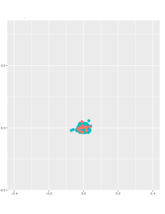
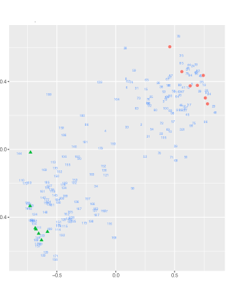
Figure 1: Estimated latent space configurations based on responses to 14 items by 200 respondents, generated by (a) the Rasch model and (b) the Rasch model with local dependence. In (a), blue circles represent respondents and red circles represent items, whereas in (b) blue numbers represent respondents, red circles represent the first 7 items, and green triangles represent the last 7 items.

To demonstrate, we conduct a simulation study. The simulation results are based on binary responses to 14 items by 200 respondents. First, data are generated from the Rasch model. Second, data are generated from the Rasch model with local dependence, that is, the responses of the first 100 respondents to the first 7 items exhibit strong local dependence in the sense of Chen  Thissen (1997), and the responses of the last 100 respondents to the last 7 items likewise exhibit strong local dependence. The proposed latent space model with $p=2$ is estimated from both datasets, using the Bayesian Markov chain Monte Carlo algorithm described in Section 3. Additional details are provided in Appendix A of the supplement. Figure 1 shows that in the first case all items and respondents are located close to the origin of $\mathbb{R}^{2}$, whereas in the second case the two groups of items are well-separated in $\mathbb{R}^{2}$ and the two groups of 100 respondents are located close to the respective sets of items, as expected.

Latent space dimension.

Throughout the remainder of the paper, we choose $\mathbb{M}=\mathbb{R}^{2}$, because a two-dimensional space has clear advantages in terms of parsimony, ease of interpretability, and visualization. As mentioned above, it is natural to interpret $\mathbb{R}^{2}$ as an interaction map rather than an ability map, because the added value of the latent space model is that it captures deviations from the main effects $\alpha_{j}$ and $\beta_{i}$ of the Rasch model – that is, interactions of respondent $j$ and item $i$ – and visualizes those interactions by embedding respondents along with items in $\mathbb{R}^{2}$.

2.2.3 Theoretical advantages

Among the theoretical advantages of the proposed latent space model is the fact that it weakens the conditional independence assumptions of conventional IRT models, along with the homogeneity assumptions of classic IRT models.

Conditional independence assumptions

The proposed latent space model is based on the following conditional independence assumption:

$$\mathbb{P}(\bm{Y}=\bm{y}\mid\mbox{\boldmath$\alpha$},\,\mbox{\boldmath$\beta$},\,\gamma,\,\bm{A},\,\bm{B})\;=\;\prod_{j=1}^{N}\,\prod_{i=1}^{I}\,\mathbb{P}(Y_{j,i}=y_{j,i}\mid\alpha_{j},\,\beta_{i},\,\gamma,\,\bm{a}_{j},\,\bm{b}_{i}),$$

where $\mbox{\boldmath$\alpha$}=(\alpha_{1},\dots,\alpha_{N})$, $\mbox{\boldmath$\beta$}=(\beta_{1},\dots,\beta_{I})$, $\bm{A}=(\bm{a}_{1},\dots,\bm{a}_{N})$, and $\bm{B}=(\bm{b}_{1},\dots,\bm{b}_{I})$. In words, the item responses are assumed to be independent conditional on the positions of respondents and items in the latent space, and the respondent and item attributes. This conditional independence assumption is weaker than the conditional independence of the Rasch model, which requires that item responses are independent conditional on respondent and item attributes. So the latent space model relaxes the conditional independence assumptions of the Rasch model and other classic IRT models.

The weaker conditional independence assumption of the latent space model allows for respondent-item interactions. As a consequence, the latent space model can account for local dependence among item responses arising from a variety of sources, including testlets (e.g., items similar in content), learning and practice effects, or repeated measurements, as well as person dependence stemming from shared school or family memberships (or even unobserved memberships).

Homogeneity assumptions

In addition, the latent space model drops some of the homogeneity assumptions made by conventional IRT models. For example, consider two respondents $j_{1}$ and $j_{2}$ with identical abilities, who are located at distances $d(\bm{a}_{j_{1}},\,\bm{b}_{i})<d(\bm{a}_{j_{2}},\,\bm{b}_{i})$ from item $i$. Then respondent $j_{1}$ has a higher probability of giving a correct response to item $i$ than respondent $j_{2}$, despite the fact that $j_{1}$ and $j_{2}$ have identical abilities. A similar scenario arises when two items $i_{1}$ and $i_{2}$ have identical difficulty levels and distances $d(\bm{a}_{j},\,\bm{b}_{i_{1}})>d(\bm{a}_{j},\,\bm{b}_{i_{2}})$ from some respondent $j$, which implies that item $i_{1}$ is less likely to be answered correctly than item $i_{2}$, despite identical difficulty levels.

Table 1: Hypothetical item response matrix consisting of four respondents 1, 2, 3, 4 and six items I1, I2, I3, I4, I5, I6. The four respondents show two response patterns. Respondents 1 and 2 give correct responses to Items I1–I3 only, whereas Respondents 3 and 4 give correct responses to Items I4–I6 only.

Response	I1	I2	I3	I4	I5	I6
1	1	1	1	0	0	0
2	1	1	1	0	0	0
3	0	0	0	1	1	1
4	0	0	0	1	1	1

To give a specific example of an educational assessment where such homogeneity assumptions are violated and to demonstrate how the latent space approach captures those violations, we provide a hypothetical item response matrix in Table 1 with six math test items answered by four respondents. Suppose the first three items are algebra items, while the last three items are geometry items. Assume that the algebra and geometry items have identical difficulty levels. Table 1 shows that Persons 1 and 2 have all algebra item correct but none of the geometry items, whereas Persons 3 and 4 have all geometry items correct but no algebra item. In other words, all respondents have three correct responses, which is an indication that all respondents have similar abilities because the difficulties of the items are the same (by assumption). However, despite similar abilities of the four respondents and identical difficulty levels of the items, it is hard to believe that the response probabilities of all respondents and all items are similar.

(a) Two response patterns	(b) Two response patterns, with randomness

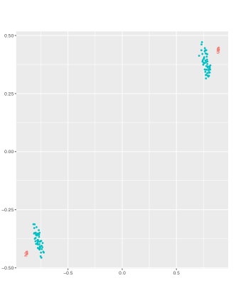
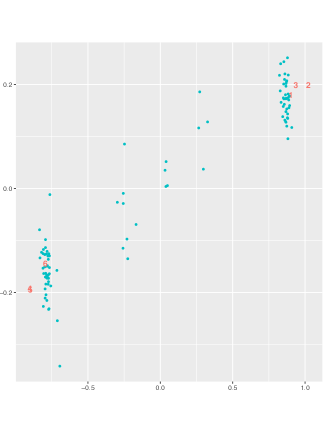
Figure 2: (a) Latent space estimated from a hypothetical data example where Respondents 1–50 (bottom left) give correct responses to Items 1–3 only, whereas Respondents 51–100 (top right) give correct responses to Items 4–6 only. $\gamma$ was estimated as 4.45 (posterior median, with 95% posterior credible interval [3.79, 5.20]). (b) Latent space estimated from a hypothetical setting similar to (a): Respondents 1–40 (bottom left) give correct responses to Items 1–3, while Respondents 41–80 (top right) give correct responses to Items 4–6. The remaining 20 respondents (middle) give random responses to Items 1–6. $\gamma$ was estimated as 3.62 [3.07, 4.26]. In both figures, blue circles represent respondents and red numbers represent items.

Figure 2(a) represents estimated latent space configurations based on item response data mimicking the item response matrix in Table 1, with 50 respondents giving correct responses to the first three items but incorrect responses to the last three items, while the other 50 respondents give incorrect responses to the first three items and correct responses to the last three items. Figure 2(b) represents estimated latent space configurations based on item response data including random response patterns – 80 respondents have response patterns similar to the response matrix in Table 1, while the other 20 respondents give random responses to Items 1–6. Figure 2 reveals that the latent space approach separates the two groups of respondents in both cases, with and without randomness. While the scenario in Figure 2(a) may be an extreme-case scenario, the scenario in Figure 2(b) is more realistic, and may very well be encountered in practice.

2.3 Related models

We review related models, excluding those we have already reviewed in Section 1.

2.3.1 Other models with relaxed assumptions

As discussed above, the proposed latent space model weakens the assumptions of classic IRT models, allowing for unobserved heterogeneity and dependence among item responses. Other approaches to relaxing those assumptions include polytomous item models, testlet and bifactor models, interaction effects models (e.g., Wainer  Kiely, 1987; Wilson  Adams, 1995), finite mixture models with latent classes (e.g., Rost, 1990), and multilevel models (e.g., Fox  Glas, 2001).

Although these approaches have been applied successfully in applications, they are not free of limitations. For instance, many of them require the dependence structure of items and respondents to be known prior to data analysis, which is a strong assumption. The latent space model does not require knowledge of the interaction structure. In addition, the discussed approaches relax some but not all of the assumptions: e.g., finite mixture models allow for heterogeneity between latent classes, but assume homogeneity within latent classes. In addition, finite mixture models assume that there are latent classes, which is equivalent to assuming that there is an unobserved, discrete metric space. In contrast, the proposed latent space model assumes that the unobserved metric space is continuous (Euclidean) rather than discrete, offering more flexibility to represent respondent-item interactions.

2.3.2 Other models with interactions among respondents and items

Two-parameter IRT model

An alternative model that captures interactions among respondents and items is the two-parameter IRT model, which assumes that

$$\mbox{logit}(\mathbb{P}(Y_{j,i}=1\mid\alpha_{j},\,\beta_{i},\,\lambda_{i}))\;=\;\lambda_{i}\;\alpha_{j}+\beta_{i},$$ (3)

where $\lambda_{i}\in\mathbb{R}$. The term $\lambda_{i}\;\alpha_{j}$ captures interactions of item $i$ and respondent $j$. The latent space approach has an important advantage over the two-parameter IRT model: It embeds both respondents and items in a low-dimensional space, helping visualize interactions of respondents and items.

Interaction IRT model

A more general interaction model assumes that

$$\mbox{logit}(\mathbb{P}(Y_{j,i}=1\mid\alpha_{j},\,\beta_{i},\,\epsilon_{j,i}))\;=\;\alpha_{j}+\beta_{i}+\epsilon_{j,i},$$ (4)

where $\epsilon_{j,i}\in\mathbb{R}$ represents the interaction of respondent $j$ and item $i$. The latent space model can be viewed as a special case of the interaction model, corresponding to

$$\epsilon_{j,i}\;=\;-\gamma\;d(\bm{a}_{j},\,\bm{b}_{i}).$$

In other words, the latent space model makes the implicit assumption that the interaction effects $\epsilon_{j,i}$ are of the form $\epsilon_{j,i}=-\gamma\;d(\bm{a}_{j},\,\bm{b}_{i})$, where the distances $d(\bm{a}_{j},\,\bm{b}_{i})$ satisfy reflexivity, symmetry, and the triangle inequality, as described in Section 2.1. While the proposed latent space model is a special case of the interaction model, it has three advantages over the interaction model. First, the latent space model can be estimated, whereas the interaction model cannot be estimated unless additional parameter constraints are imposed, because in practice we have a single observation (i.e., item response) for each pair of respondents and items. Second, the latent space model captures transitivity in item response data thanks to the triangle inequality: e.g., if the positions of two respondents $j_{1}$ and $j_{2}$ are close to the position of item $i$ in the latent space, then the two respondents are fairly close to each other, by the triangle inequality; likewise, if two items $i_{1}$ and $i_{2}$ are close to respondent $j$, then the two items are fairly close to each other. The assumption that item response data are transitive makes sense in applications. Therefore, while the latent space model is more restrictive than the general interaction model, the restrictions make sense in practice, and facilitate estimation. Last, but not least, the latent space approach provides an interaction map of respondents and items.

Bilinear mixed effects models and related models

The multiplicative effects version of the latent space model is related to the bilinear mixed effects model of Hoff (2005), the additive and multiplicative effects models of Hoff (2020), and the latent factor models of Agarwal  Chen (2009). For example, the bilinear mixed effects models of Hoff (2005) are models of network data, such as friendships among $N$ students. Bilinear mixed effects models add a multiplicative effect of the form $\bm{a}_{j}^{\top}\,\bm{b}_{i}$ to the log odds of a friendship between students $i$ and $j$. The multiplicative effects version of the proposed latent space models resembles the multiplicative effects in the above-mentioned models, but multiplicative effects are more difficult to interpret, as mentioned at the beginning of Section 2.

Differential item functioning

Last, but not least, IRT models for studying differential item functioning (DIF) can be seen as special cases of interaction models, where an interaction term is formed with a known categorical attribute of respondents (e.g., gender) and an item indicator. Conventional DIF models, however, require pre-knowledge of the respondent attribute. The proposed latent space model does not require such pre-knowledge.

3 Bayesian inference

3.1 Markov chain Monte Carlo (MCMC)

We propose a fully Bayesian approach for estimating the proposed latent space model, using MCMC methods. Bayesian inference is preferable to maximum likelihood due to under-identification of the latent space positions.

We use the following priors:

$$\begin{array}[]{llllllllll}\alpha_{j}\mid\sigma^{2}&\mathop{\rm\sim}\limits^{\mbox{\tiny ind}}&\mbox{N}\left(0,\,\sigma^{2}\right),\;\;\;\;\sigma^{2}>0,\;\;\;\;j=1,\dots,N\vspace{.25cm}\\ \beta_{i}\mid\tau^{2}_{\beta}&\mathop{\rm\sim}\limits^{\mbox{\tiny ind}}&\mbox{N}\left(0,\,\tau^{2}_{\beta}\right),\;\;\;\;\tau_{\beta}^{2}>0,\;\;\;\;i=1,\dots,I\vspace{.25cm}\\ \log\gamma\mid\mu_{\gamma},\,\tau^{2}_{\gamma}&\sim&\mbox{N}\left(\mu_{\gamma},\,\tau^{2}_{\gamma}\right),\;\;\;\;\mu_{\gamma}\in\mathbb{R},\;\;\;\;\tau^{2}_{\gamma}>0\vspace{.25cm}\\ \sigma^{2}\mid a_{\sigma},\,b_{\sigma}&\sim&\mbox{Inv-Gamma}\left(a_{\sigma},\,b_{\sigma}\right),\;\;\;\;a_{\sigma}>0,\;\;\;\;b_{\sigma}>0\vspace{.25cm}\\ \bm{a}_{j}&\mathop{\rm\sim}\limits^{\mbox{\tiny iid}}&\mbox{MVN}_{p}\left(\bm{0},\,\bm{I}_{p}\right),\;\;\;\;j=1,\dots,N\vspace{.25cm}\\ \bm{b}_{i}&\mathop{\rm\sim}\limits^{\mbox{\tiny iid}}&\mbox{MVN}_{p}\left(\bm{0},\,\bm{I}_{p}\right),\;\;\;\;i=1,\dots,I,\end{array}$$

where $\bm{0}$ is a $p$-vector of zeroes and $\bm{I}_{p}$ is the $p\times p$ identity matrix. In principle, it is possible to specify priors of distances directly rather than indirectly (i.e., by specifying priors of positions). However, specifying a prior for distances is more challenging than specifying a prior for positions, because the distances must satisfy the triangle inequality. As a consequence, it is conventional in the latent space model literature to place a prior on positions rather than distances, and we follow here convention. We use $\tau^{2}_{\beta}=4$, $a_{\sigma}=1$, $b_{\sigma}=1$, $\mu_{\gamma}=0.5$, $\tau^{2}_{\gamma}=1$, which are not uncommon in the literature (see, e.g., Furr ., 2016). While these priors may seem strong, note that the effective parameter space of many models for binary item response data is small: e.g., when item responses are independent Bernoulli$(\pi)$ random variables with success probability $\pi\in(0,1)$ and log odds $\alpha=\mbox{\rm logit}(\pi)\in\mathbb{R}$, then values of $\alpha$ outside of the interval $[-5,+5]$ correspond to probabilities close to $0$ or $1$, which are unrealistic. Therefore, while the theoretical parameter space of $\alpha$ is $\mathbb{R}$, the effective parameter space is a subset of $\mathbb{R}$, e.g., $[-5,+5]$. As a consequence, using priors that place most probability mass on $[-5,+5]$ are reasonable, and so are the priors suggested above. The priors described above are used throughout the remainder of the paper, unless stated otherwise.

The posterior of the parameters $\bm{\alpha}$, $\bm{\beta}$, and $\gamma$ and the unobserved positions of respondents $\bm{A}$ and items $\bm{B}$, given an observation $\bm{y}$ of $\bm{Y}$, is proportional to

$$\begin{array}[]{lllll}f(\bm{\alpha},\;\bm{\beta},\;\gamma,\;\bm{A},\;\bm{B}\mid\bm{y})&\propto&\left[\displaystyle\prod_{j=1}^{N}f(\alpha_{j})\right]\;\left[\displaystyle\prod_{i=1}^{I}f(\beta_{i})\right]\;f(\gamma)\;\left[\displaystyle\prod_{j=1}^{N}f(\bm{a}_{j})\right]\;\left[\displaystyle\prod_{i=1}^{I}f(\bm{b}_{i})\right]\vspace{.25cm}\vspace{.25cm}\\ &\times&\left[\displaystyle\prod_{j=1}^{N}\displaystyle\prod_{i=1}^{I}\mathbb{P}\Big{(}Y_{j,i}=y_{j,i}\mid\alpha_{j},\;\beta_{i},\;\gamma,\;\bm{a}_{j},\;\bm{b}_{i}\Big{)}\right],\end{array}$$ (5)

where, in an abuse of notation, we use $f(.)$ to denote the prior and posterior probability density functions of the parameters as well as the positions of respondents and items.

We sample from the posterior by using an MCMC algorithm that updates the parameters and the positions of respondents and items at iteration $t$ as follows:

1. Propose $\alpha_{j}^{\star}$ from a symmetric proposal distribution and accept the proposal with probability

   $$\min\left(1,\;\frac{f\Big{(}\alpha_{j}^{\star}\mid\mbox{$\mathbf{y}$},\,\bm{A},\,\bm{B},\,\mbox{\boldmath$\beta$},\,\gamma\Big{)}}{f\Big{(}\alpha_{j}^{(t)}\mid\mbox{$\mathbf{y}$},\,\bm{A},\,\bm{B},\,\mbox{\boldmath$\beta$},\,\gamma\Big{)}}\right).$$

2. Propose $\beta_{i}^{\star}$ from a symmetric proposal distribution and accept the proposal with probability

   $$\min\left(1,\;\frac{f\Big{(}\beta_{i}^{\star}\mid\mbox{$\mathbf{y}$},\,\bm{A},\,\bm{B},\,\mbox{\boldmath$\alpha$},\,\gamma\Big{)}}{f\Big{(}\beta_{i}^{(t)}\mid\mbox{$\mathbf{y}$},\,\bm{A},\,\bm{B},\,\mbox{\boldmath$\alpha$},\,\gamma\Big{)}}\right).$$

3. Propose $\gamma^{\star}$ from a symmetric proposal distribution and accept the proposal with probability

   $$\min\left(1,\;\frac{f\Big{(}\gamma^{\star}\mid\mbox{$\mathbf{y}$},\,\bm{A},\,\bm{B},\,\mbox{\boldmath$\alpha$},\,\mbox{\boldmath$\beta$}\Big{)}}{f\Big{(}\gamma^{(t)}\mid\mbox{$\mathbf{y}$},\,\bm{A},\,\bm{B},\,\mbox{\boldmath$\alpha$},\,\mbox{\boldmath$\beta$}\Big{)}}\right).$$

4. Propose $\bm{a}_{j}^{\star}$ from a symmetric proposal distribution and accept the proposal with probability

   $$\min\left(1,\;\frac{f\Big{(}\bm{a}_{j}^{\star}\mid\mbox{$\mathbf{y}$},\,\bm{A}_{-j},\,\bm{B},\,\mbox{\boldmath$\alpha$},\,\mbox{\boldmath$\beta$},\,\gamma\Big{)}}{f\Big{(}\bm{a}_{j}^{(t)}\mid\mbox{$\mathbf{y}$},\,\bm{A}_{-j},\,\bm{B},\,\mbox{\boldmath$\alpha$},\,\mbox{\boldmath$\beta$},\,\gamma\Big{)}}\right),$$

   where $\bm{A}_{-j}=(\bm{a}_{1},\dots,\bm{a}_{j-1},\bm{a}_{j+1},\dots,\bm{a}_{N})$.

5. Propose $\bm{b}_{i}^{\star}$ from a symmetric proposal distribution and accept the proposal with probability

   $$\min\left(1,\;\frac{f\Big{(}\bm{b}_{i}^{\star}\mid\mbox{$\mathbf{y}$},\,\bm{A},\,\bm{B}_{-i},\,\mbox{\boldmath$\alpha$},\,\mbox{\boldmath$\beta$},\,\gamma\Big{)}}{f\Big{(}\bm{b}_{i}^{(t)}\mid\mbox{$\mathbf{y}$},\,\bm{A},\,\bm{B}_{-i},\,\mbox{\boldmath$\alpha$},\,\mbox{\boldmath$\beta$},\,\gamma\Big{)}}\right),$$

   where $\bm{B}_{-i}=(\bm{b}_{1},\dots,\bm{b}_{i-1},\bm{b}_{i+1},\dots,\bm{b}_{I})$.

6. Sample $\sigma^{2}$ from its full conditional distribution:

   $$\sigma^{2}\sim\mbox{Inv-Gamma}\left(a_{\sigma}+\frac{N}{2},\;b_{\sigma}+\frac{\sum_{j=1}^{N}\alpha_{j}^{2}}{2}\right).$$

As symmetric proposal distributions, we use (multivariate) Gaussian distributions centered at the current values of the parameters or the positions of respondents and items, with diagonal variance-covariance matrices. The variances of the (multivariate) Gaussians are set to achieve a good performance of the algorithm (with an acceptance rate of 0.3). To detect non-convergence of the MCMC algorithm, we use trace plots along with the Gelman-Rubin diagnostic (Gelman  Rubin, 1992). The MCMC algorithm was written in R. The R code, along with an example dataset, can be found in the supplementary materials.

3.2 Identifiability

The log odds of a correct response is invariant to translations, reflections, and rotations of the positions of respondents and items, because the log odds depends on the positions through the distances, and the distances are invariant under the said transformations. As a consequence, the likelihood function is invariant under the same transformations. The same form of identifiability issue arises in latent space models of network data (Hoff ., 2002). Such identifiability issues can be resolved by post-processing the MCMC output with Procrustes matching (Gower, 1975). However, the results need to be interpreted with care, because there are many latent space configurations that give rise to the same distances. So an estimated latent space should be interpreted in terms of the relative distances between positions, rather than the actual positions.

3.3 Model Selection

In practice, given a dataset, it is natural to ask: Did the Rasch model with $\gamma=0$ or the latent space model with $\gamma>0$ generate the data? If the latent space model generated the data, it is appropriate to base conclusions regarding respondents and items on the latent space model, including the interaction map provided by the latent space model. Otherwise the Rasch model suffices.

To determine whether the Rasch model with $\gamma=0$ or the latent space model with $\gamma>0$ generated the data, we use a model selection approach based on spike-and-slab priors (Ishwaran  Rao, 2005). We specify a spike-and-slab prior for $\log\gamma$ by specifying a prior consisting of two component distributions: a spike prior $N_{spike}(\mu_{\gamma_{0}},\,\tau^{2}_{\gamma_{0}})$ with a small variance $\tau^{2}_{\gamma_{0}}>0$ that places most of its probability mass in a small neighborhood of $0$, and a slab prior $N_{slab}(\mu_{\gamma_{1}},\,\tau^{2}_{\gamma_{1}})$ with a large variance $\tau^{2}_{\gamma_{1}}>0$ that distributes its probability mass across the parameter space. In other words, the prior of $\log\gamma$ may be expressed as

$$\log\gamma\;\sim\;(1-\delta)\;N_{spike}(\mu_{\gamma_{0}},\,\tau^{2}_{\gamma_{0}})+\delta\;N_{slab}(\mu_{\gamma_{1}},\,\tau_{\gamma_{1}}^{2}),$$

where $\delta\in\{0,1\}$. If the posterior probability of the event $\delta=0$ is less than $0.5$, we choose the Rasch model with $\gamma=0$, otherwise we choose the latent space model with $\gamma>0$. The posterior probability can be approximated by the proportion of times we observe the event $\delta=1$ in a Markov chain Monte Carlo sample from the posterior. We choose as a prior for $\omega=p(\delta=1\mid\omega)\in[0,1]$ the $\mbox{Beta}(1,\,1)$ distribution. As a spike prior, we use $N_{spike}(-3,\,1)$, so that the distribution of $\log\gamma\mid\delta=0$ has mode $0.02$, mean $0.08$, and standard deviation $0.01$. As a slab prior, we use $N_{spike}(0.5,\,1)$, with mode $.0.61$, mean $2.72$, and standard deviation $3.56$. As pointed out in Section 3.1, the effective parameter space of many models for binary item response data is small, so the slab prior is not unreasonable.

The model selection method described is applied to the two real data applications provided in Section 4. We evaluate the accuracy of the model selection method via simulations in Section 5.

4 Applications

To demonstrate the latent space approach, we provide two empirical examples.

4.1 Example 1: Attitudes to Abortion

4.1.1 Data and Estimation

As a first example, we used the attitudes-to-abortion scale that came from Social and community planning research (1987). Seven items were included in the scale, which ask respondents whether abortion should be legal in each of the following seven scenarios:

1. The woman decides on her own that she does not wish to have the child

2. The couple agree that they do not wish to have the child

3. The woman is not married and does not wish to marry the man

4. The couple cannot afford any more children.

5. There is a strong chance of a defect in the baby

6. The woman’s health is seriously endangered by the pregnancy

7. The woman became pregnant as a result of rape

Binary responses to the seven items were collected, where response ‘Yes’ was coded as 1 and response ‘No’ was coded as 0. The mean proportion of ‘Yes’ was 0.42, 0.52, 0.47, and 0.53 for Items 1 to 4, while 0.86, 0.94, and 0.93 for Items 5 to 7, respectively ($N$=642). The positive response proportion was quite high for the last three items that describe rather extreme situations in which most respondents are likely to endorse. To implement MCMC, we specified the priors as we described in Section 3. For $\beta$, we chose a stronger prior with $\tau^{2}_{\beta}=1$ because otherwise the MCMC did not converge well due to the boundary effects of probability for Items 5-7 (the positive answer probability was too close to 1). We selected the tuning parameters (standard deviations of the proposal distributions) to ensure a reasonable acceptance rate as follows: 2.2 for $\alpha_{j}$, 0.5 for $\beta_{i}$, 0.1 for $\gamma$, 1.7 for $\bm{a}_{j}$, and 0.4 for $\bm{b}_{i}$. The MCMC run included 20,000 iterations with the first 10,000 iterations discarded as a burn-in period. The computation took approximately 28 minutes for the latent space model on a standard computer. Trace plots showed reasonable convergence of the sampler (convergence evidence was provided in Appendix B of the supplement). In addition, we used the Gelman-Rubin diagnostic (Gelman  Rubin, 1992) to detect possible non-convergence. We ran the model with three sets of random starting values; the scale reduction factor was smaller than 1.06 for all model parameters, suggesting that there are no signs of non-convergence. We implemented the model selection method with the spike-and-slab prior, described in Section 3.3. The posterior inclusion probability of $\delta$ was .99, in favor of the proposed model to the Rasch model. Hence, we move forward with the latent space item response model for the current application.

4.1.2 Results

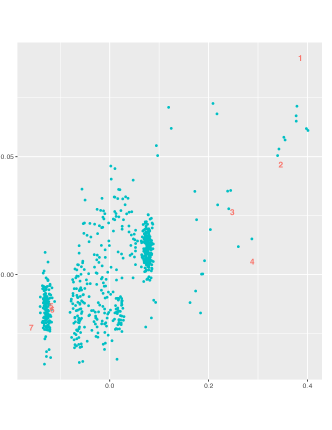
Figure 3: Estimated latent space for the attitudes to abortion data. Red numbers represent items and blue dots represent respondents.

Interpreting latent space results

Figure 3 displays the estimated latent space. This latent space shows the point estimates (posterior means) of the positions but not their uncertainty, for the ease of visualization. Uncertainty of the estimated positions, measured with the 95% posterior credible intervals, is reported in Appendix C of the supplement. The $\gamma$ parameter was estimated as 1.25 (posterior median, with 95% posterior credible interval [0.92, 1.54]) and $\sigma$ as 2.34 (posterior median, with 95% posterior credible interval [2.07, 2.62]).

Roughly two item groups appear in the latent space; one group with three items in the bottom left of the space (Items 5–7) and the other group with four items in the top right side of the space (Items 1–4). Also, two respondent groups appear, with a larger group in the left bottom part of the space (near Items 5–7) and a much smaller, scattered group on the right upper side of the space (near Items 1–4). Respondents close to Items 1–4 but apart from Items 5–7 tend to give positive responses to the mild items (Items 1–4) but negative responses to the extreme items (Items 5–7). Table 2 shows that the respondents in the region of $X>0.3$ and $Y>0.025$ (close to Items 1-4) indeed tend to choose YES to Items 1 to 4 but NO to Items 5 to 7. Respondents close to Items 5–7 tend to give positive responses to the extreme items but negative responses to the mild situations (Items 1–4).

Table 2: Response patterns to Items 1 to 7 (I1 to I7) for respondents (ID) in the smaller person cluster, located in the bottom left corner of the latent space (which is the region of $X>0.3$ and $Y>0.025$). These people tend to give positive responses to I1–I4, but negative responses to I5–I7.

ID	I1	I2	I3	I4	I5	I6	I7
27	1	0	0	1	0	0	0
92	1	1	1	1	1	0	0
132	1	1	0	1	0	0	0
191	1	1	1	1	0	1	0
273	1	1	0	0	0	0	0
330	1	0	0	1	0	0	0
653	1	1	0	1	0	0	0
662	1	1	1	0	0	0	0
675	1	1	1	0	0	0	0

Comparison with the Rasch model

(a) LS $\beta_{i}$	(b) Rasch $\beta_{i}$
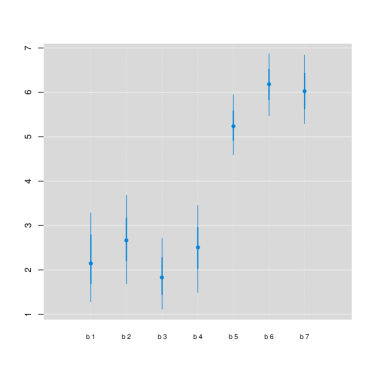
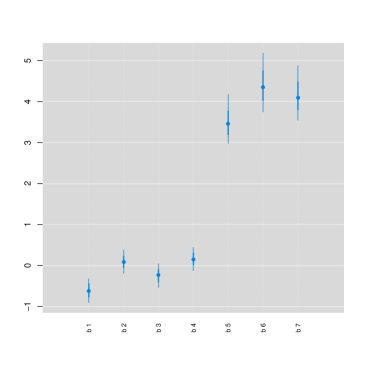
(c) LS $\alpha_{j}$	(d) Rasch $\alpha_{j}$

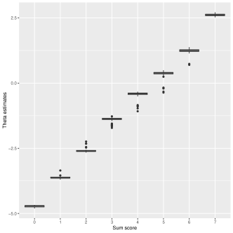
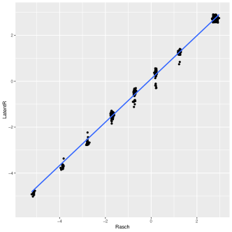
Figure 4: (a) and (b) show the 95% posterior credible intervals for $\beta$ for Items 1 to 7 (indicated by b1 to b7) from the latent space model (LS) and the Rasch model for the attitudes to abortion data. (c) shows the box plot of $\alpha$ estimates per total sum score on the X-axis (0 to 7) from the latent space model. (d) shows $\alpha$ estimates between the Rasch model (Rasch, X-axis) and the latent space model (LatentR, Y-axis).

We compared our parameter estimates with those from the Rasch model (Equation 1). The Rasch model was estimated with the fully Bayesian approach with the same set of priors as our model’s for the $\beta_{i}$, $\alpha_{j}$, $\sigma^{2}$ parameters. Estimation details were provided in Appendix D of the supplement.

From the Rasch model, $\sigma$ was estimated as 2.40 (posterior median, with 95% posterior credible interval [1.87, 3.02]), similar to the latent space IRT model estimate (2.34 with [2.07, 2.62]). The item parameter estimates ($\beta_{i}$) are displayed in Figure 4(a) and (b). The item parameter estimates from the Rasch model appear smaller by a constant (approximately 2 in the logit scale) compared with the latent space model, which is sensible given that the proposed model has the additional penalty term (distances).

We then compared the person parameter estimates ($\alpha_{j}$) in Figure 4(c) and (c). Overall, the estimates under these two models are similar, with a rank order correlation of .95. It is noteworthy that $\alpha_{j}$ rarely change much compared to the Rasch model, whereas $\beta_{i}$ alters due to the added latent space term. This is another evidence that the latent space is not the ability space, at least in this example.

Posterior predictive checking

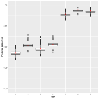
Figure 5: Predicted proportions of the positive responses for the seven items for the attitudes to abortion data. The red dot in each box indicates the proportion of positive responses calculated from the raw data.

We evaluated the absolute goodness-of-fit of the proposed latent space model based on posterior predictive checking. We compared the proportions of correct responses between the observed data and the replicated datasets (based on the estimated model parameters). Little discrepancy between the observed and replicated measures indicates satisfactory goodness-of-fit of the model. Figures 5 displays the box plots of the predicted proportions of positive responses for the seven items over 10,000 replicated data. The red dot in each box indicates the observed proportion. The predicted measures show highly congruent behavior to the observed measure, suggesting reasonable goodness-of-fit of the proposed model to the data under investigation. Further, based on Cohen’s $d$ effect size, no item showed large mean differences between the replicated and original data with the proposed model ($|d|>0.8$).

4.2 Example 2: Deductive Reasoning

4.2.1 Data and Estimation

As a second example, we used the data from the Competence Profile Test of Deductive Reasoning – Verbal assessment (DRV; Spiel ., 2001; Spiel  Gluck, 2008). This dataset was analyzed in Jin  Jeon (2019), allowing us to compare ours to the results from the NIRM approach. The DRV test was developed to measure deductive reasoning of children in different developmental stages and includes 24 binary items (0 = correct, 1 = incorrect), which fall into three broad categories: (1) Type of inference (four levels: Modus Ponens (MP), Modus Tolens (MT), Negation of Antecedent (NA), and Affirmation of Consequence (AC)); (2) Content of conditional (three levels: Concrete (CO), Abstract (AB), and Counterfactual (CF)); and (3) Precedent of antecedent (two levels: No Negation (UN) and Negation (N)). More details are provided in Appendix E of the supplement.

The data include item responses from 418 school students, 162 female and 256 male students from grade 7 to 12. The success rate ranged from 0.19 to 0.85 with a mean of 0.53 for the 24 test items. The MCMC algorithm described in Section 3 was used to sample from the posterior. The standard deviations of the proposal distributions were selected to ensure a reasonable acceptance rate as follows: 0.4 for $\beta$, 1.4 for $\alpha$, 0.05 for $\gamma$, 1.1 for $a$ and 0.4 for $b$. We generated 20,000 MCMC iterations, discarding the first 10,000 iterations as burn-in. The computing time was about 56 minutes. The trace plots do not show obvious signs of non-convergence (Appendix F of the supplement). As an additional guard against non-convergence, we used the Gelman-Rubin diagnostic. To do so, we ran the MCMC algorithm with three sets of starting values chosen at random. We found that the scale reduction factor was less than 1.1 for all parameters, so there were no signs of non-convergence. The model selection method described in Section 3.3 was used to determine whether the dataset was generated by the Rasch model with $\gamma=0$ or the latent space model with $\gamma>0$. A posterior probability of more than $.99$ in favor of the latent space model suggests that the latent space model generated the data, so all following results are based on the latent space model.

4.2.2 Results

Parameter estimates

Figures 6(a) and (b) show the 95% posterior credible intervals for the $\beta_{i}$ estimates of the 24 items and the distribution of the $\alpha_{j}$ estimates per total test score. The $\beta_{i}$ estimates ranged from 1 to 7 and the $\alpha_{j}$ estimates ranged from -2 to 2. The $\alpha_{j}$ estimates were generally aliened well with the total scores. The latent position estimates, posterior means and 95% posterior credible intervals, are provided in Appendix G of the supplement. The $\gamma$ parameter was estimated as 2.23 (posterior median, with 95% posterior credible interval [2.08, 2.35]) and $\sigma$ as 2.51 [2.27, 2.76].

(a) $\beta_{i}$	(b) $\alpha_{j}$

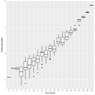
Figure 6: (a) 95% posterior credible intervals for the $\beta_{i}$ estimates (b1 and b24 on the X-axis represent Items 1 to 24), and (b) the distribution of the $\alpha_{j}$ estimates per total test score for the DRV data. The estimates are from the latent space model.

Posterior predictive checking

Goodness of fit of the latent space model was evaluated with posterior predictive checking. Figure 7 displays the box plots of the predicted correct response proportions over 10,000 replicated responses for the 24 DRV test items from the proposed model. The red dot in each box indicates the correct response proportion from the original data. The result shows that the prediction of our proposed model was excellent, supporting satisfying goodness of fit of the proposed model. Based on Cohen’s $d$ effect size, no item showed large mean differences from the original data with the proposed model ($|d|>0.8$).

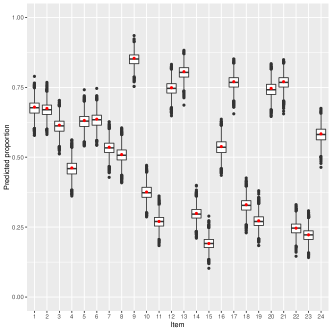
Figure 7: Box plots of the predicted proportions of the correct responses for the 24 DRV test items from 10,000 replicated data. The red dot in each box indicates the proportion of the correct responses for the corresponding item from the raw data.

Item structure

Figure 8(a) displays the estimated latent space, where bullet points represent respondents and numbers represent items. Roughly, four item groups appear as color-coded for distinction. The four item group members are listed in Table 3. The item structure identified here shows an excellent agreement with the structure identified in Jin  Jeon (2019) based on the NIRM approach.

(a) DRV latent space	(b) with item group vectors

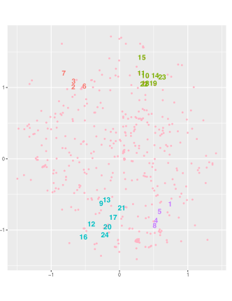
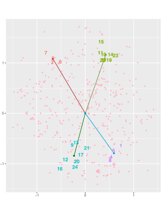
Figure 8: (a) Latent space for the DRV data and (b) DRV data latent space superimposed with the four vectors that represent the centers of four item groups (I1, I2, I3, and I4). In both figures, dots represent respondents and numbers represent items. Four item groups are distinguished with four different colors. I1: Items 2,3,6,7; I2: Items 10,11,14,15,18,19,22,23; I3: Items 9,12,13,16,17,20,21,24; I4: Items 1,4,5,8.

Item group	Group details
I1	UN_CO_NA (2); UN_CO_AC (3); N_CO_NA (6); N_CO_AC (7)
I2	UN_AB_NA (10); UN_AB_AC (11); N_AB_NC (14); N_AB_AC (15);
	UN_CF_NA (18); UN_CF_AC (19); N_CF_NA (22); N_CF_MT (23)
I3	UN_AB_MP (9); UN_AB_MT (12); N_AB_MP (13); N_AB_MT (16);
	UN_CF_MP (17); UN_CF_MT (20); N_CF_MP (21); N_CF_MT (24)
I4	UN_CO_MP (1); UN_CO_MT (4); N_CO_MP (5); N_CO_MT (8)

Table 3: Members of the four item groups identified in the DRV data latent space. Numbers in parenthesis indicate item numbers. The acronyms in the item labels indicate the following design factors and their levels: (1) UN vs. N: no negation (UN) and Negation (N) for the presentation of the antecedent factor. (2) CO vs. AB vs. AC: Concrete (CO), Abstract (AB), and Counterfactual (CF) for the content of conditional factor. (3) MP vs. MT vs. NA vs. AC: Modus Ponens (MP), Modus Tollens (MT), Negation of Antecednet (NA), and Affirmation of Consequent (AC) for the type of inference factor.

I1 and I2 in the upper part of the latent space consist of Concrete items (CO). They are further differentiated in terms of Type of Inference; I1 on the left includes bi-conditional inference items (MP and MT) and I2 on the right includes more complex inference type items (NA and AC). I3 and I4 in the bottom part of the latent space consist of logical fallacy items (Ab and CF). They are further separated by Type of Inference; I3 on the left includes bi-conditional items (MP and MT) and I4 on the right includes complex algebra items (NA and AC). The Presentation of Antecedent factor (UN vs. N) is mixed in all groups, meaning that this factor hardly contributes to item differentiation.

Success probabilities for item group

We assessed the correct response probabilities within and between the four identified item groups (I1, I2, I3, and I4). The density plots of the log odds success probabilities of the individual items per item group are presented in Figure 9. While the four groups show different patterns of the logit success probabilities, items within the same group are similar in the patterns.

(a) Item group l1	(b) Item group l2
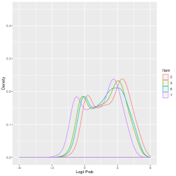
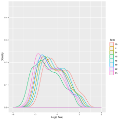
(c) Item group l3	(d) Item group l4

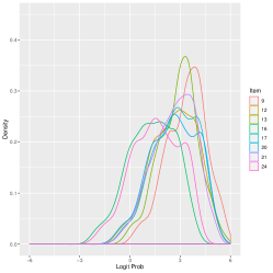
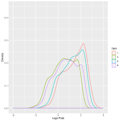
Figure 9: Density plots of the log odds success probabilities of the individual DRV test items per item group. (a) to (d) represent the density plots for item groups I1 to I4 groups in order. I2: Items 10,11,14,15,18,19,22,23; I3: Items 9,12,13,16,17,20,21,24; I4: Items 1,4,5,8.

Cosine similarity between item groups

We evaluated similarities between two positions in a latent space by the cosine similarity measure. The cosine similarity of two vectors $\bm{a}\in\mathbb{R}^{p}$ and $\bm{b}\in\mathbb{R}^{p}$ of length $||\bm{a}||_{2}>0$ and $||\bm{b}||_{2}>0$ was computed as

$$\begin{array}[]{ccc}\cos(\theta)&=&\dfrac{\bm{a}^{\top}\,\bm{b}}{||\bm{a}||_{2}\;||\bm{b}||_{2}},\end{array}$$

where $\theta$ is the angle between two vectors $\bm{a}$ and $\bm{b}$. The cosine similarity measure takes on values in the interval $[-1,1]$. Two vectors pointing into the same direction have a cosine similarity of 1, two vectors with opposite directions have a cosine similarity of -1, and two orthogonal vectors have a cosine similarity of 0.

While cosine similarity can be computed between any two positions in a latent space – including positions of items, respondents, and both items and respondents – we focus here on similarities between the four item groups. Figure 8(b) shows the original DRV latent space added with the four vectors indicating the centers of the four item groups (where the centers are the mean positions of the corresponding item group members). Table 4 presents a matrix of cosine similarity measures between the four item groups.

	I1	I2	I3	I4
I1	-
I2	0.618	-
I3	-0.680	-0.996	-
I4	-0.996	-0.546	0.613	-

Table 4: Cosine similarity measures between (centers of) the four item groups. I1: Items 2,3,6,7; I2: Items 10,11,14,15,18,19,22,23; I3: Items 9,12,13,16,17,20,21,24; I4: Items 1,4,5,8.

Table 4 confirms that I1 is most dissimilar to I4 and I2 is most dissimilar to I3. Marked dissimilarities between I1 and I4 and between I2 and I3 support our earlier finding that Type of Inference (MP/MT vs. NA/AC) most substantially differentiates the DRV test items.

Respondent structure

To evaluate their performance in the latent space, we first categorized the children into four sub-groups based on their proximity to the four item groups:

1. Children near I1. They performed well on logical fallacy inference items (NA/AC) but poorly with simpler inference items (MP/NT) when the items involved concrete conditionals (Co);

2. Children near I2. They performed well on logical fallacy inference items (NA/AC) but poorly with simpler inference items (MP/NT) if the items involved abstract or counterfactual conditionals (NA/AC);

3. Children near I3. They performed well on simpler inference items (MP/MT) but poorly with logical fallacy inference items (NA/AC) if the items involved abstract or counterfactual conditionals (NA/AC);

4. Children near I4. They performed well on simpler inference items (MP/MT) but poorly with logical fallacy inference items (NA/AC) if the items involved concrete conditionals (Co);

Based on the above, we can reasonably conclude that children in sub-groups 3 and 4 were at a lower level of deductive reasoning than those children in sub-groups 1 and 2. While performing well with complex inference items, children in sub-groups 1 and 2 showed poor performance on simpler inference items. This indicates that they might be in a transition to a higher developmental stage. Children in a transition stage tend to make mistakes with easier items, for instance, due to over-generalization on simple problems (e.g., Markovits ., 1998; Draney, 2007)

Further, it is possible to make additional sub-grouping of children. For instance,

1. Children between I1 and I3. They were good with both simple and logical fallacy inference items when the items were combined with abstract/counterfactual and concrete conditionals, respectively;

2. Children between I2 and I4. They were good with both simple and logical fallacy inference items when the items were combined with concrete and abstract/counterfactual conditionals, respectively;

3. Children around the center of the latent space. They performed equally well on most test items.

How can we identify a specific sub-group for each respondent? One could draw a contour that represents a 95% posterior credible region for each child. If the contours of children overlap, the children may form a subgroup of children that are similar. In addition, one can directly calculate a distance between an individual respondent and each item or item group. For instance, suppose respondent A has a distance of 0.5 from I1, 1.5 from I2, 2 from I3, and 3 from I4. That is, the ratio or relative distances is 1:3:4:, meaning that respondent A belongs to the subgroup near I1. So, it is possible to categorize respondents based on their quantified relative distances.

Comparisons with principal component analysis and factor analysis

Our model showed that items in the same item group are similar, while items in different groups are distinctive in terms of contents as well as success probabilities. Traditional methods, such as principal component analysis (PCA) and factor analysis (FA), might be used for similar purposes.

(a) PCA	(b) Factor analysis

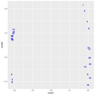
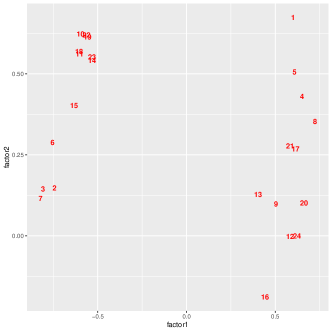
Figure 10: (a) Principal component analysis (PCA) solution with a tetrachoric correlation matrix as input and (b) item factor analysis (FA) solution with oblim rotation for the DRV data.

To compare, we applied PCA and FA to the DRV data where two principal components and two factors were extracted. The solutions from the two methods are presented in Figure 10. Items are placed in the two-dimensional spaces that represent the two principal components or factors. The item clusters identified with PCA and FA are roughly similar to our approach. With factor analysis, the membership of a few items, such as Items 6, 15, 17, and 21, were less clear compared with the other approaches. However, two important differences need to be clarified: (1) in the two traditional methods, extracting factors or principal components (dimensions) is often the main interest, whereas it is not the case in our approach; (2) both in PCA and FA, items and respondents cannot be placed in the same space, unlike our approach.

Latent space rotation

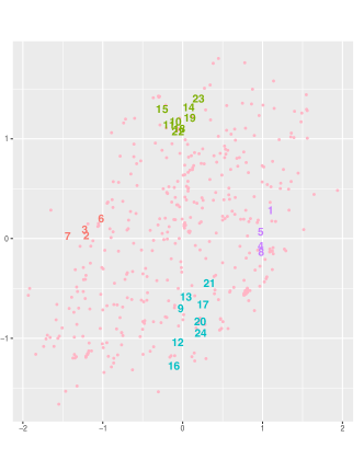
Figure 11: Rotated latent space for the DRV data with oblim rotation. Dots represent respondents and numbers represent items. Four item groups are distinguished with four different colors. I1: Items 2,3,6,7; I2: Items 10,11,14,15,18,19,22,23; I3: Items 9,12,13,16,17,20,21,24; I4: Items 1,4,5,8.

When desirable, we can attach substantive interpretations to latent space dimensions based on neighboring items. To illustrate, we return to the original latent space displayed in Figure 8(a). No items appear close to the X-axis; therefore, it is difficult to interpret the X-axis in a meaningful way.

To improve interpretability, we rotate the original latent space to a place where items are better encompassed by the axes, which is permitted due to rotational invariance property of latent space. Rotation is a frequently utilized technique in factor analysis which also has rotational invariance. We applied oblim rotation (Jennrich, 2002) to the estimated item position matrix $\bm{B}$ using the R package GPArotation (Bernaards  Jennrich, 2005), and then rotated the respondent position matrix $\bm{B}$ in the same way with a common rotation matrix. We denote the rotated item and respondent position matrices by $\bm{A}^{*}$ and $\bm{B}^{*}$, respectively.

Figure 11 displays the rotated latent space for the DRV data. Two item groups I1 and I4 are positioned close to the X-axis, while I2 and I3 are placed close to the Y-axis in the rotated space. This indicates that the X-axis represents Type of Inference (MP/MT vs. NA/AC) combined with Concrete conditionals, while the Y-axis represents Type of Inference (MP/MT vs. NA/AC) combined with Abstract and Counterfactual conditionals. Items are differentiated based on the type of inference in each dimension, while the two dimensions are separated by the content of conditionals (concrete vs. abstract/counterfactual).

5 Simulation Study

We conducted a simulation study to evaluate whether the model selection approach described in Section 3.3 can determine if the Rasch model with $\gamma=0$ or the latent space model with $\gamma>0$ generated a given dataset. To do so, we used the setting of Figure 1(a) and 1(b) with $N=200$ and $I=14$. We simulated 100 datasets under the Rasch model with $\gamma=0$ and under the latent space model with $\gamma=1.7$. For each simulated dataset, the MCMC algorithm was run for 5,000 burn-in iterations, followed by 5,000 post-burn-in iterations. We estimated the posterior probability of the indicator $\delta=1$ by the proportion of times $\delta=1$ in a Markov chain Monte Carlo sample from the posterior.

(a) Truth: $\gamma=0$	(b) Truth: $\gamma=1.7$

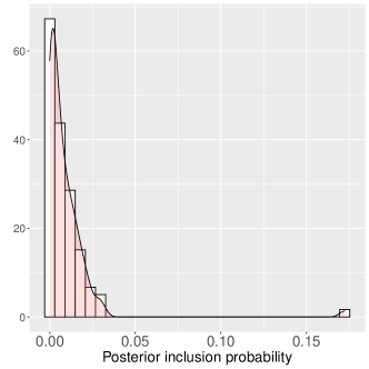
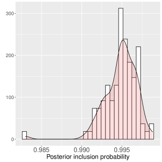
Figure 12: Histogram of the estimated posterior probability of the event $\delta=1$, called “posterior inclusion probability.” (a) Data are generated from the Rasch model with $\gamma=0$. (b) Data are generated from the latent space model with $\gamma=1.7$.

Figure 12 shows a histogram of the estimated posterior probability of the event $\delta=1$. In Figure 12(a), data are generated from the Rasch model with $\gamma=0$. The posterior probability of $\delta=1$ is smaller than 0.05 in at least 99% of the simulated data sets. In Figure 12(b), data are generated from the latent space model with $\gamma=1.7$. Here, the posterior inclusion probability of $\delta=1$ is greater than 0.99 in at least 99% of the simulated data sets. If the Rasch model is chosen when the estimated posterior probability of $\delta=1$ is less than $0.5$ and otherwise the latent space model is chosen, then the data-generating model is selected in all simulated data sets.

These simulation results provide reasonable evidence that the proposed model selection approach helps determine whether the Rasch model with $\gamma=0$ or the latent space model with $\gamma>0$ generated a given dataset. In other words, the model selection approach helps decide whether the Rasch model suffices or whether there are systematic deviations from the Rasch model due to unobserved respondent-item interactions, which the latent space model can capture and represent in a low-dimensional space.

6 Discussion

6.1 Summary

We have introduced a novel approach to modeling item response data, capturing deviations from the Rasch model in the form of respondent-item interactions. While the Rasch model is a classic model and may be a natural starting point in practice, many item response datasets can be expected to exhibit deviations from the respondent and item effects of the Rasch model, which implies that there are unexplained interactions between items and respondents. We have presented evidence of interactions in two empirical examples, but in a number of other datasets we tested, we likewise observed that interactions among respondents and items are present and non-negligible. We propose to capture deviations from the Rasch model in the form of respondent-item interactions by embedding both respondents and items in a low-dimensional latent space, which represents interactions between items, between respondents, and between items and respondents that are not explained by the Rasch model. The proposed latent space approach has technical advantages over conventional IRT modeling approaches, because it makes weaker independence and conditional assumptions than conventional approaches, such as the Rasch model. An additional, intriguing advantage is that it produces a geometrical representation of items and respondents that can provide important insights into how respondents perform on test items.

6.2 Some final thoughts on practical advantages and possible applications

We mention here some final thoughts on practical advantages and possible applications of the proposed latent space approach. First and foremost, if the model selection approach described in Section 3.3 determines that $\gamma>0$, then the data exhibit systematic deviations from the main effects of the Rasch model, that is, respondent-item interactions. The estimated latent space supplies an interaction map that represents those deviations in a low-dimensional space, providing diagnostic feedback on items as well as respondents. For example, the estimated latent space may be useful for assessing whether test items are differentiated or grouped together as blueprinted by test developers: e.g., the DRV test was developed based on three design factors, and we found that one design factor (the Presentation of Antecedent) barely contributed to item differentiation and could be dropped without much loss.

In addition, the estimated latent space could help detect unintended or undesirable forms of test-taking behavior. For instance, suppose that a computer-based cognitive test with a time constraint is administered (without permission to skip items) and the estimated latent space reveals that a group of respondents is located close to the last test items in the latent space. That may be an unintended consequence of the fact that most test takers ran out of time and did not respond to the last test items, so that the few respondents who did respond to them are close to those items in the latent space. It goes without saying that such conclusions need to be accompanied by additional evidence (e.g., item response times), but the latent space approach can nonetheless be helpful for diagnosing problems in the first place.

Last, but not least, the proposed latent space approach is useful for providing feedback on the test performance of individual test takers or subgroups of test takers. For example, in the DRV example, we have demonstrated that one can identify items that individual test takers may be struggling with. Such information could guide classroom instruction, and help evaluate and improve intervention programs.

References

- Agarwal \BBA Chen (\APACyear2009) \APACinsertmetastaragarwal:09{APACrefauthors}Agarwal, D.\BCBT \BBA Chen, B\BHBIC. \APACrefYearMonthDay2009. \BBOQ\APACrefatitleRegression-based latent factor models Regression-based latent factor models.\BBCQ \APACjournalVolNumPagesProceedings of the 15th ACM SIGKDD international conference on Knowledge discovery and data mining19-28. \PrintBackRefs\CurrentBib
- Bates \BOthers. (\APACyear2015) \APACinsertmetastarbates:15{APACrefauthors}Bates, D., Mächler, M., Bolker, B.\BCBL \BBA Walker, S. \APACrefYearMonthDay2015. \BBOQ\APACrefatitleFitting Linear Mixed-Effects Models Using lme4 Fitting linear mixed-effects models using lme4.\BBCQ \APACjournalVolNumPagesJournal of Statistical Software6711–48. {APACrefDOI} \doi10.18637/jss.v067.i01 \PrintBackRefs\CurrentBib
- Bernaards \BBA Jennrich (\APACyear2005) \APACinsertmetastarbernaards:05{APACrefauthors}Bernaards, C\BPBIA.\BCBT \BBA Jennrich, R\BPBII. \APACrefYearMonthDay2005. \BBOQ\APACrefatitleGradient Projection Algorithms and Software for Arbitrary Rotation Criteria in Factor Analysis Gradient projection algorithms and software for arbitrary rotation criteria in factor analysis.\BBCQ \APACjournalVolNumPagesEducational and Psychological Measurement65676–696. \PrintBackRefs\CurrentBib
- Borsboom (\APACyear2008) \APACinsertmetastarBo08{APACrefauthors}Borsboom, D. \APACrefYearMonthDay2008. \BBOQ\APACrefatitlePsychometric Perspectives on Diagnostic Systems Psychometric perspectives on diagnostic systems.\BBCQ \APACjournalVolNumPagesJournal of Clinical Psychology6491089–1108. \PrintBackRefs\CurrentBib
- Chalmers (\APACyear2012) \APACinsertmetastarchalmers:12{APACrefauthors}Chalmers, R\BPBIP. \APACrefYearMonthDay2012. \BBOQ\APACrefatitlemirt: A Multidimensional Item Response Theory Package for the R Environment mirt: A multidimensional item response theory package for the R environment.\BBCQ \APACjournalVolNumPagesJournal of Statistical Software4861–29. \PrintBackRefs\CurrentBib
- Chen \BBA Thissen (\APACyear1997) \APACinsertmetastarchen:97{APACrefauthors}Chen, W\BHBIH.\BCBT \BBA Thissen, D. \APACrefYearMonthDay1997. \BBOQ\APACrefatitleLocal dependence indexes for item pairs using item response theory Local dependence indexes for item pairs using item response theory.\BBCQ \APACjournalVolNumPagesJournal of Educational and Behavioral Statistics22265-289. \PrintBackRefs\CurrentBib
- Draney (\APACyear2007) \APACinsertmetastardraney:07{APACrefauthors}Draney, K. \APACrefYearMonthDay2007. \BBOQ\APACrefatitleThe Saltus model applied to proportional reasoning data The Saltus model applied to proportional reasoning data.\BBCQ \APACjournalVolNumPagesJournal of Applied Measurement8438–455. \PrintBackRefs\CurrentBib
- Epskamp \BOthers. (\APACyear2018) \APACinsertmetastarEpskamp:2018{APACrefauthors}Epskamp, S., Borsboom, D.\BCBL \BBA Fried, E\BPBII. \APACrefYearMonthDay2018. \BBOQ\APACrefatitleEstimating psychological networks and their accuracy: A tutorial paper Estimating psychological networks and their accuracy: A tutorial paper.\BBCQ \APACjournalVolNumPagesBehavior Research Methods50195-212. \PrintBackRefs\CurrentBib
- Fox \BBA Glas (\APACyear2001) \APACinsertmetastarfox:01{APACrefauthors}Fox, J\BPBIP.\BCBT \BBA Glas, C\BPBIA. \APACrefYearMonthDay2001. \BBOQ\APACrefatitleBayesian estimation of a multilevel IRT model using Gibbs sampling Bayesian estimation of a multilevel IRT model using Gibbs sampling.\BBCQ \APACjournalVolNumPagesPsychometrika66271-288. \PrintBackRefs\CurrentBib
- Furr \BOthers. (\APACyear2016) \APACinsertmetastarfurr:16{APACrefauthors}Furr, D\BPBIC., Lee, S\BHBIY., Lee, J\BHBIH.\BCBL \BBA Rabe-Hesketh, S. \APACrefYearMonthDay2016. \APACrefbtitleTwo-Parameter Logistic Item Response Model – STAN. https://mc-stan.org/users/documentation/case-studies/tutorial_twopl.html. Two-parameter logistic item response model – STAN. https://mc-stan.org/users/documentation/case-studies/tutorial_twopl.html. \PrintBackRefs\CurrentBib
- Gelman \BBA Rubin (\APACyear1992) \APACinsertmetastargelman:92{APACrefauthors}Gelman, A.\BCBT \BBA Rubin, D\BPBIB. \APACrefYearMonthDay1992. \BBOQ\APACrefatitleInference from iterative simulation using multiple sequences Inference from iterative simulation using multiple sequences.\BBCQ \APACjournalVolNumPagesiterative simulation using multiple sequences. Statistical Science7457–472. \PrintBackRefs\CurrentBib
- Goodfellow \BOthers. (\APACyear2016) \APACinsertmetastarGoodfellow-et-al-2016{APACrefauthors}Goodfellow, I., Bengio, Y.\BCBL \BBA Courville, A. \APACrefYear2016. \APACrefbtitleDeep Learning Deep learning. \APACaddressPublisherMIT Press. \PrintBackRefs\CurrentBib
- Gower (\APACyear1975) \APACinsertmetastarGower:1975{APACrefauthors}Gower, J\BPBIC. \APACrefYearMonthDay1975. \BBOQ\APACrefatitleGeneralized procrustes analysis Generalized procrustes analysis.\BBCQ \APACjournalVolNumPagesPsychometrika4033–51. \PrintBackRefs\CurrentBib
- Hoff (\APACyear2005) \APACinsertmetastarhoff:05{APACrefauthors}Hoff, P. \APACrefYearMonthDay2005. \BBOQ\APACrefatitleBilinear mixed-effects models for dyadic data Bilinear mixed-effects models for dyadic data.\BBCQ \APACjournalVolNumPagesJournal of the American Statistical Association286-295. \PrintBackRefs\CurrentBib
- Hoff (\APACyear2020) \APACinsertmetastarHo18{APACrefauthors}Hoff, P. \APACrefYearMonthDay2020. \BBOQ\APACrefatitleAdditive and multiplicative effects network models Additive and multiplicative effects network models.\BBCQ \APACjournalVolNumPagesStatistical Science. \APACrefnoteto appear \PrintBackRefs\CurrentBib
- Hoff \BOthers. (\APACyear2002) \APACinsertmetastarHoff:2002{APACrefauthors}Hoff, P., Raftery, A.\BCBL \BBA Handcock, M\BPBIS. \APACrefYearMonthDay2002. \BBOQ\APACrefatitleLatent space approaches to social network analysis Latent space approaches to social network analysis.\BBCQ \APACjournalVolNumPagesJournal of the American Statistical Association971090-1098. \PrintBackRefs\CurrentBib
- Ishwaran \BBA Rao (\APACyear2005) \APACinsertmetastarIshwaran:05{APACrefauthors}Ishwaran, H.\BCBT \BBA Rao, J\BPBIS. \APACrefYearMonthDay2005. \BBOQ\APACrefatitleSpike and slab variable selection: Frequentist and Bayesian strategies Spike and slab variable selection: Frequentist and Bayesian strategies.\BBCQ \APACjournalVolNumPagesThe Annals of Statistics33730-773. \PrintBackRefs\CurrentBib
- Jennrich (\APACyear2002) \APACinsertmetastarJennrich:02{APACrefauthors}Jennrich, R\BPBII. \APACrefYearMonthDay2002. \BBOQ\APACrefatitleA simple general method for oblique rotation A simple general method for oblique rotation.\BBCQ \APACjournalVolNumPagesPsychometrika677-19. \PrintBackRefs\CurrentBib
- Jin \BBA Jeon (\APACyear2019) \APACinsertmetastarJin:18{APACrefauthors}Jin, I\BPBIH.\BCBT \BBA Jeon, M. \APACrefYearMonthDay2019. \BBOQ\APACrefatitleA Doubly Latent Space Joint Model for Local Item and Person Dependence in the Analysis of Item Response Data A doubly latent space joint model for local item and person dependence in the analysis of item response data.\BBCQ \APACjournalVolNumPagesPsychometrika84236-260. \PrintBackRefs\CurrentBib
- Jin \BOthers. (\APACyear2018) \APACinsertmetastarJin:2018b{APACrefauthors}Jin, I\BPBIH., Jeon, M., Schweinberger, M.\BCBL \BBA Lin, L. \APACrefYearMonthDay2018. \BBOQ\APACrefatitleHierarchical Network Item Response Modeling for Discovering Differences Between Innovation and Regular School Systems in Korea Hierarchical network item response modeling for discovering differences between innovation and regular school systems in Korea.\BBCQ \APACjournalVolNumPagesAvailable at arxiv.org/abs/1810.07876. \PrintBackRefs\CurrentBib
- Lauritzen (\APACyear1996) \APACinsertmetastarLa96{APACrefauthors}Lauritzen, S. \APACrefYear1996. \APACrefbtitleGraphical Models Graphical models. \APACaddressPublisherOxford, UKOxford University Press. \PrintBackRefs\CurrentBib
- Markovits \BOthers. (\APACyear1998) \APACinsertmetastarmarkovits:98{APACrefauthors}Markovits, H., Fleury, M\BHBIL., Quinn, S.\BCBL \BBA Venet, M. \APACrefYearMonthDay1998. \BBOQ\APACrefatitleThe development of conditional reasoning and the structure of semantic memory The development of conditional reasoning and the structure of semantic memory.\BBCQ \APACjournalVolNumPagesChild Development69742–755. \PrintBackRefs\CurrentBib
- Marsman \BOthers. (\APACyear2018) \APACinsertmetastarMarsman:2018{APACrefauthors}Marsman, M., Borsboom, D., Kruis, J., Epskamp, S., van Bork, R., Waldorp, L\BPBIJ.\BDBLMaris, G\BPBIK\BPBIJ. \APACrefYearMonthDay2018. \BBOQ\APACrefatitleAn introduction to Network Psychometrics: Relating Ising network models to item response theory models An introduction to network psychometrics: Relating ising network models to item response theory models.\BBCQ \APACjournalVolNumPagesMultivariate Behavioral Research5315-35. \PrintBackRefs\CurrentBib
- McCullagh \BBA Nelder (\APACyear1983) \APACinsertmetastarMpNj83{APACrefauthors}McCullagh, P.\BCBT \BBA Nelder, J\BPBIA. \APACrefYear1983. \APACrefbtitleGeneralized linear models Generalized linear models. \APACaddressPublisherLondonChapman & Hall. \PrintBackRefs\CurrentBib
- Pearl (\APACyear1988) \APACinsertmetastarPe88{APACrefauthors}Pearl, J. \APACrefYear1988. \APACrefbtitleProbabilistic Reasoning in Intelligent Systems: Networks of Plausible Inference Probabilistic reasoning in intelligent systems: Networks of plausible inference. \APACaddressPublisherSan FranciscoMorgan Kaufmann. \PrintBackRefs\CurrentBib
- Rasch (\APACyear1961) \APACinsertmetastarRasch:1961{APACrefauthors}Rasch, G. \APACrefYearMonthDay1961. \BBOQ\APACrefatitleOn general laws and meaning of measurement in psychology On general laws and meaning of measurement in psychology.\BBCQ \BIn \APACrefbtitleProceedings of the Fourth Berkeley Symposium on Mathematical Statistics and Probability (Volume 4) Proceedings of the fourth berkeley symposium on mathematical statistics and probability (volume 4) (\BPG 321-333). \PrintBackRefs\CurrentBib
- Revelle (\APACyear2019) \APACinsertmetastarrevelle:19{APACrefauthors}Revelle, W. \APACrefYearMonthDay2019. \BBOQ\APACrefatitlepsych: Procedures for Psychological, Psychometric, and Personality Research psych: Procedures for psychological, psychometric, and personality research\BBCQ [\bibcomputersoftwaremanual]. \APACaddressPublisherEvanston, Illinois. {APACrefURL} \urlhttps://CRAN.R-project.org/package=psych \APACrefnoteR package version 1.9.12 \PrintBackRefs\CurrentBib
- Rost (\APACyear1990) \APACinsertmetastarrost:90{APACrefauthors}Rost, J. \APACrefYearMonthDay1990. \BBOQ\APACrefatitleRasch Models in Latent Classes: An Integration of Two Approaches to Item Analysis Rasch models in latent classes: An integration of two approaches to item analysis.\BBCQ \APACjournalVolNumPagesApplied Psychological Measurement14271–282. \PrintBackRefs\CurrentBib
- Schweinberger \BBA Snijders (\APACyear2003) \APACinsertmetastarSchweinberger:03{APACrefauthors}Schweinberger, M.\BCBT \BBA Snijders, T\BPBIA\BPBIB. \APACrefYearMonthDay2003. \BBOQ\APACrefatitleSettings in social networks: A measurement model Settings in social networks: A measurement model.\BBCQ \BIn R\BPBIM. Stolzenberg (\BED), \APACrefbtitleSociological Methodology Sociological methodology (\BVOL 33, \BPGS 307–341). \APACaddressPublisherBoston & OxfordBasil Blackwell. \PrintBackRefs\CurrentBib
- Sewell \BBA Chen (\APACyear2015) \APACinsertmetastarsewell2015latent{APACrefauthors}Sewell, D\BPBIK.\BCBT \BBA Chen, Y. \APACrefYearMonthDay2015. \BBOQ\APACrefatitleLatent space models for dynamic networks Latent space models for dynamic networks.\BBCQ \APACjournalVolNumPagesJournal of the American Statistical Association1101646–1657. \PrintBackRefs\CurrentBib
- Skrondal \BBA Rabe-Hesketh (\APACyear2004) \APACinsertmetastarskrondal:04{APACrefauthors}Skrondal, A.\BCBT \BBA Rabe-Hesketh, S. \APACrefYear2004. \APACrefbtitleGeneralized Latent Variable Modeling: Multilevel, Longitudinal, and Structural Equation Models Generalized Latent Variable Modeling: Multilevel, Longitudinal, and Structural Equation Models. \APACaddressPublisherBoca Raton, FLChapman & Hall/CRC. \PrintBackRefs\CurrentBib
- Smith \BOthers. (\APACyear2019) \APACinsertmetastarSmAsCa19{APACrefauthors}Smith, A\BPBIL., Asta, D\BPBIM.\BCBL \BBA Calder, C\BPBIA. \APACrefYearMonthDay2019. \BBOQ\APACrefatitleThe geometry of continuous latent space models for network data The geometry of continuous latent space models for network data.\BBCQ \APACjournalVolNumPagesStatistical Science34428–453. \PrintBackRefs\CurrentBib
- Social and community planning research (\APACyear1987) \APACinsertmetastarPlanning:1987{APACrefauthors}Social and community planning research. \APACrefYear1987. \APACrefbtitleBritish Social Attitude, the 1987 Report British social attitude, the 1987 report. \APACaddressPublisherGower Publishing, Aldershot. \PrintBackRefs\CurrentBib
- Spiel \BBA Gluck (\APACyear2008) \APACinsertmetastarspiel:08{APACrefauthors}Spiel, C.\BCBT \BBA Gluck, J. \APACrefYearMonthDay2008. \BBOQ\APACrefatitleA model based test of competence profile and competence level in deductive reasoning A model based test of competence profile and competence level in deductive reasoning.\BBCQ \BIn J. Hartig, E. Klieme\BCBL \BBA D. Leutner (\BEDS), \APACrefbtitleAssessment of competencies in educational contexts: State of the art and future prospects Assessment of competencies in educational contexts: State of the art and future prospects (\BPG 41-60). \APACaddressPublisherGottingenHogrefe. \PrintBackRefs\CurrentBib
- Spiel \BOthers. (\APACyear2001) \APACinsertmetastarspiel:01{APACrefauthors}Spiel, C., Gluck, J.\BCBL \BBA Gossler, H. \APACrefYearMonthDay2001. \BBOQ\APACrefatitleStability and change of unidimensionality: The sample case of deductive reasoning Stability and change of unidimensionality: The sample case of deductive reasoning.\BBCQ \APACjournalVolNumPagesJournal of Adolescent Research16150-168. \PrintBackRefs\CurrentBib
- Wainer \BBA Kiely (\APACyear1987) \APACinsertmetastarwainer:87{APACrefauthors}Wainer, H.\BCBT \BBA Kiely, G\BPBIL. \APACrefYearMonthDay1987. \BBOQ\APACrefatitleItem clusters and computerized adaptive testing: A case for testlets Item clusters and computerized adaptive testing: A case for testlets.\BBCQ \APACjournalVolNumPagesJournal of Educational Measurement24185-201. \PrintBackRefs\CurrentBib
- Wasserman \BBA Faust (\APACyear1994) \APACinsertmetastarWsFk94{APACrefauthors}Wasserman, S.\BCBT \BBA Faust, K. \APACrefYear1994. \APACrefbtitleSocial Network Analysis: Methods and Applications Social network analysis: Methods and applications. \APACaddressPublisherCambridgeCambridge University Press. \PrintBackRefs\CurrentBib
- Wilson \BBA Adams (\APACyear1995) \APACinsertmetastarwilson:95{APACrefauthors}Wilson, M.\BCBT \BBA Adams, R\BPBIJ. \APACrefYearMonthDay1995. \BBOQ\APACrefatitleRasch models for item bundles Rasch models for item bundles.\BBCQ \APACjournalVolNumPagesPsychometrika60181-198. \PrintBackRefs\CurrentBib