Dirac Polarons and Resistivity Anomaly in $\mathrm{ZrTe}_{5}$ and $\mathrm{HfTe}_{5}$

Abstract

Resistivity anomaly, a sharp peak of resistivity at finite temperatures, in the transition-metal pentatellurides $\mathrm{ZrTe_{5}}$ and $\mathrm{HfTe_{5}}$ was observed four decades ago, and more exotic and anomalous behaviors of electric and thermoelectric transport were revealed recent years. Here we present a theory of Dirac polarons, composed by massive Dirac electrons and holes in an encircling cloud of lattice displacements or phonons at finite temperatures. The chemical potential of Dirac polarons sweeps the band gap of the topological band structure by increasing the temperature, leading to the resistivity anomaly. Formation of a nearly neutral state of Dirac polarons accounts for the anomalous behaviors of the electric and thermoelectric resistivity around the peak of resistivity.

Introduction

Resistivity in the transition-metal pentatellurides $\mathrm{ZrTe}_{5}$ and $\mathrm{HfTe}_{5}$ exhibits a sharp peak at a finite temperature $T_{p}$. The peak occurs approximately at a large range of temperatures from 50 to 200K, but the exact value varies from sample to sample. The effect was observed forty years ago (okada1980giant, ; izumi1981anomalous, ), but has yet to be understood very well. At the beginning, it was thought as a structural phase transition, or occurrence of charge density wave. The idea was soon negated as no substantial evidence is found to support the picture (disalvo1981possible, ; okada1982negative, ; bullett1982absence, ; fjellvag1986structural, ). The measurements of the Hall and Seebeck coefficients showed that the type of charge carriers dominating the electrical transport changes its sign around the peak, which indicates the chemical potential of the charge carriers sweeps band gap around the transition temperature $T_{p}$ (izumi1982hall, ; jones1982thermoelectric, ; littleton1999transition, ; tritt1999enhancement, ). Thus the anomaly is believed to originate in the strong temperature dependence of the chemical potential and carrier mobility. Recent years the advent of topological insulators revives extensive interests to explore the physical properties of $\mathrm{ZrTe}_{5}$ and $\mathrm{HfTe}_{5}$. The first principles calculation suggested that the band structures of $\mathrm{ZrTe}_{5}$ and $\mathrm{HfTe}_{5}$ are topologically nontrivial in the layered plane or very close to the topological transition points (weng2014transition, ). Further studies uncover more exotic physics in these compounds (chen2017spectroscopic, ; manzoni2016evidence, ; jiang2020unraveling, ; chen2015optical, ; li2016chiral, ; Zhou2016Pressure, ; Li2018Giant, ; Wang2018Discovery, ; liang2018anomalous, ; wang2019log, ; Zhang2019anomalous, ; tang2019three, ; Hu2019Large, ; wang2020quantum, ), such as the chiral magnetic effect and three-dimensional quantum Hall effect. Other possible causes have been advanced much recently (Zhao2017anomalous, ; PhysRevX.8.021055, ; xu2018temperature, ), but the physical origin of the resistivity anomaly is still unclear. For example, it was suggested that a topological quantum phase transition might occur, and the gap closing and reopening give rise to the resistivity anomaly (xu2018temperature, ). However it contradicts with the observation of the angle-resolved photoemission spectroscopy (ARPES) measurement (zhang2017electronic, ; zhang2017temperature, ).

Strong temperature dependence of the band structure (zhang2017electronic, ) implies that the interaction between the Bloch electrons and the lattice vibrations, i.e., electron-phonon interaction (EPI), is an indispensable ingredient to understand the anomaly (rubinstein1999hfte, ). In this Letter, we consider an anisotropic Dirac model describing the low energy excitations of weak topological insulator near the Fermi surface and EPI in $\mathrm{ZrTe_{5}}$ and $\mathrm{HfTe_{5}}$, and propose a theory of Dirac polarons for the resistivity anomaly at finite temperatures. The Dirac polarons are mixtures of massive Dirac electrons and holes encircling a cloud of phonons, and are the effective charge carriers in the compounds. Increasing temperature will change the overlapping of the Dirac polarons drastically. The chemical potential of Dirac polarons sweeping the band gap from conduction bands to valence bands with increasing the temperature. Consequently, when the chemical potential of Dirac polarons locates around the middle of the band gap, the resistivity is enhanced drastically to form a pronounced peak at a finite temperature. The carriers dominated the charge transport change the sign around the transition. The formation of a nearly neutral state of Dirac polarons accounts for anomalous electric and magneto transport properties in the compounds.

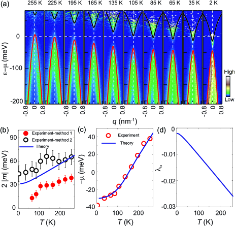
Figure 1: (a) A comparison of the renormalized energy spectrums according to the theory (the solid lines) and the temperature-dependent band structures from ARPES measurement adopted from Fig. 2(b) in Ref. (zhang2017electronic, ). (b) The renormalized Dirac mass $m$ due to the EPI , (c) the temperature dependent chemical potential $\mu$, and (d) the velocity dressing function $\lambda_{\alpha}$. The experiment data are extracted from Fig.2(d) and (f) in Ref. (zhang2017electronic, ). The model parameters are set to be $v_{x}\simeq v_{y}=v_{\perp}=4\times 10^{5}\mathrm{m}/s$, $v_{z}=0.5\times 10^{5}m/s$, $b_{x}\simeq b_{y}=b_{\perp}=230\mathrm{meV}\mathrm{nm}^{2}$, $d_{x}\simeq d_{z}=d_{\perp}=-225\mathrm{meV}\mathrm{nm}^{2}$, $b_{z}=d_{z}=0$ and $m=12.0\,\mathrm{meV}$ for all the figures if there is no further claiming. The carrier density used here is $n=4\times 10^{17}\mathrm{cm^{-3}}$.

Finite temperature spectral function and quasiparticle properties

The charge carriers in the conduction and valence bands of the bulk $\mathrm{ZrTe_{5}}$ and $\mathrm{HfTe_{5}}$ are strongly coupled together due to spin-orbit interaction and behave like massive Dirac fermions instead of conventional electrons in semiconductors and metals (Wu2016evidence, ; Li2016Experimental, ; manzoni2016evidence, ). In the following, we only focus on $\mathrm{ZrTe_{5}}$ for comparison with experimental measurement and theoretical calculation without loss of generality. When the electrons (or holes) are moving through the ionic lattices, the surrounding lattice will be displaced from the original equilibrium positions; consequently, the electrons (or holes) will be encircled by the lattice distortions, or phonons. At finite temperatures, Dirac polarons are composed of both massive Dirac electrons and holes in a cloud of phonons due to the thermal activation when the chemical potential is located around the band edges as illustrated in Fig.1(A). The Hamiltonian describing the EPI in Dirac materials has the form (Mahan-book, ), $\mathcal{H}_{tot}=\mathcal{H}_{Dirac}+\mathcal{H}_{ph}+\mathcal{H}_{ep}$. Here the phonon part $\mathcal{H}_{ph}$ is in the harmonic approximation, and the EPI part $\mathcal{H}_{ep}$ is dominantly contributed by longitudinal acoustic phonons. The low-energy physics of the electronic states near the Fermi surface $\mathcal{H}_{Dirac}$, can be well described by the anisotropic Dirac model (SQS, ),

$$\mathcal{H}_{Dirac}(\mathbf{p})=(d(\mathbf{p})-\mu)I+\sum_{i=x,y,z}\hbar v_{i}p_{i}\alpha_{i}+m(\mathbf{p})\beta,$$ (1)

where $\mathbf{p}=(p_{x},p_{y},p_{z})$ is the relative momentum to the $\Gamma$ point, $v_{i}$ ($i=x,y,z$) are the effective velocities in three directions. $\mu$ is the chemical potential. $d(\mathbf{p})=\sum_{i=x,y,z}d_{i}p_{i}^{2}$ breaks the particle-hole symmetry, and plays essential role in the Dirac polaron physics. $m(\mathbf{p})=m-\sum_{i=x,y,z}b_{i}p_{i}^{2}$ is the momentum dependent Dirac mass. The first principles calculation suggested that $\mathrm{ZrTe_{5}}$ is possibly a weak topological insulator (weng2014transition, ), and the ARPES measurement showed that there is no surface states within the band gap in its a-c plane (the layers stacking along the b axis) (weng2014transition, ). Thus, we consider an anisotropic case of $b_{x}\simeq b_{y}>0$ and $b_{z}\leq 0$. The detailed analysis of the band topology can be found in Sec. SI of Ref. (Note-on-SM, ) . The Dirac matrices are chosen to be $\boldsymbol{\alpha}=\tau_{x}\otimes(\sigma_{x},\sigma_{y},\sigma_{z})$ and $\beta=\tau_{z}\otimes\sigma_{0}$, where $\sigma$ and $\tau$ are the Pauli matrices acting on spin and orbital space, respectively. The quantitative information about these physical properties, such as the Dirac velocity, the Dirac mass or the energy gap can be extracted from the ARPES data (Manzoni2015ultrafast, ; Moreschini2016nature, ; zhang2017electronic, ). To explore the EPI effect, we treat $\mathcal{H}_{ep}$ as a perturbation to either electrons or phonons in the Migdal approximation (Migdal-58jetp, ) that the self-energy arises from the virtual exchange of a phonon at temperature $T$. Due to the spinor nature of Dirac electrons, the retarded self-energy can be recast in a matrix form as (Note-on-SM, ; Garate2013phonon, ; Saha2014phonon, )

$$\Sigma_{ep}^{R}(\mathbf{p},\epsilon)=\Sigma_{I}(\mathbf{p},\epsilon)+\lambda_{\alpha}(\mathbf{p},\epsilon)\hbar v\mathbf{p}\cdot\boldsymbol{\alpha}+\Sigma_{\beta}(\mathbf{p},\epsilon)\beta,$$ (2)

where $\Sigma_{I}(\mathbf{p},\epsilon)$ is the renormalization to the chemical potential $\mu$,$\lambda_{\alpha}(\mathbf{p},\epsilon)$ is the velocity dressing function and $\Sigma_{\beta}(\mathbf{p},\epsilon)$ is the renormalization to the Dirac mass $m$.

The quasiparticle properties of Dirac polaron can be obtained by the poles of the retarded Green’s function $G^{R}(\mathbf{p},\epsilon)=[\epsilon-\mathcal{H}_{Dirac}(\mathbf{p})-\Sigma^{R}(\mathbf{p},\epsilon)]^{-1}$, which is in the complex plane with its real part gives the spectrum of the quasiparticle and the imaginary part gives its lifetime. The self-energy $\Sigma^{R}(\mathbf{p},\epsilon)=\Sigma_{ep}^{R}(\mathbf{p},\epsilon)+\Sigma_{imp}^{R}(\mathbf{p},\epsilon)$ includes the contribution from the impurities scattering. The spectral function of the quasiparticle properties of Dirac polarons is given by the imaginary part of $G^{R}(\mathbf{p},\epsilon)$,

$$A_{\zeta}(\mathbf{p},\epsilon)=-\frac{1}{\pi}\langle\zeta s\mathbf{p}|\mathrm{Im}G^{R}(\mathbf{p},\epsilon)|\zeta s\mathbf{p}\rangle\text{,}$$ (3)

where $|\zeta s\mathbf{p}\rangle$ are the band states with the band indices $\zeta=\pm$ for the conduction and valence band and spin indices $s=\pm$. In the absence of disorder and EPI, $A_{\zeta}(\mathbf{p},\epsilon)$ is a $\delta$ function reflecting that $\mathbf{p}$ is a good quantum number and all its weight ratio is precisely at $\epsilon=\xi_{\mathbf{p}}^{\zeta}$. In the presence of disorder and EPI, at low temperatures, $A_{\zeta}(\mathbf{p},\epsilon)$ exhibits a sharp peak of the Lorentzian type due to a long lifetime. As temperature increases, $A_{\zeta}(\mathbf{p},\epsilon)$ maintains the Lorentzian line shape but becomes broader due to the increasing of the scattering rate, and the peak position moves to the positive energy due to the renormalization of the energy level. The trajectories of the peaks of the spectral function give us the renormalized dispersion $\widetilde{\xi}_{\zeta}(\mathbf{p})$. As shown in Fig. 1(a), we plot the derived energy dispersions $\widetilde{\xi}_{\zeta}(\mathbf{p})$ for different temperatures with the black and red lines corresponding the conduction and valence band respectively. The ARPES data extracted from Ref. (zhang2017electronic, ) are also presented as the background for a comparison. The excellent agreement can be found between our theoretical calculations and the experiment data. The overall band structure shifts up to higher energy with increasing temperature. The peak structure of the spectral function can be clearly observed in the temperature range considered, which suggests that a quasiparticle picture is still appropriate at low energy and the EPI largely preserving the weakly perturbed Fermi-liquid behavior.

The renormalized Dirac mass $m$ is given by the difference between two energy levels $\widetilde{\xi}_{+}(\mathbf{0})$ and $\widetilde{\xi}_{-}(\mathbf{0})$ for the states at the band edge ($\mathbf{p}=0$):$\bar{m}=\frac{1}{2}[\widetilde{\xi}_{+}(\mathbf{0})-\widetilde{\xi}_{-}(\mathbf{0})]$. At higher temperature, the effective mass varies with $T$ as $\bar{m}\simeq m+g_{m}T$ shown in Fig. 1(b). The coefficient $g_{m}$ are determined by the band structure and the EPI strength (see the details in Ref.(Note-on-SM, )). For Dirac materials, the renormalization of the energy levels is attributed to the contributions from both intra- and inter-band scatterings. With increasing the temperature, the more phonon modes with high momenta are active, the larger the renormalization is. The chemical potential is determined by the charge carriers density $n=\int_{|\bar{m}|}^{\infty}d\omega\left[\bar{\nu}_{+}(\omega)n_{F}(\omega-\mu)-\bar{\nu}_{-}(-\omega)n_{F}(\omega+\mu)\right]$ where $n_{F}(x)=[\exp(x/k_{B}T)+1]^{-1}$ is the Fermi distribution function and $\bar{\nu}_{\pm}(\omega)$ are the renormalized density of states for the conduction and valence band, respectively. In the band structure of $\mathrm{ZrTe_{5}}$, the particle-hole symmetry is broken and the valence band is narrower than the conduction band. At the fixed $n$, the temperature dependence $\mu(T)$ are plotted in Fig. 1(c). The calculated results demonstrate that the chemical potential sweeps over the energy band gap of the massive Dirac particles with increasing the temperature. At low temperatures, $\mu(T)\approx\mu(0)-\frac{\pi^{2}}{6}(k_{B}T)^{2}\frac{d\bar{\nu}_{\pm}(\omega)/d\omega}{\bar{\nu}_{\pm}(\omega)}\Big{|}_{\omega=\mu(0)}$shows a quadratic temperature dependence by means of the Sommerfeld expansion. $\mu(T)=0$ means the chemical potential is located at the mid-gap, which approximately defines the transition temperature $T_{p}$ around. At high temperatures, due to the strong particle-hole asymmetry and the relatively low carrier density, the chemical potential shifts into the valence band in a relatively linear fashion with increasing the temperature. The velocity dressing function $\lambda_{\alpha}$ as a function of $T$ is plotted in Fig. 1(d). The velocity for Dirac polaron decreases linearly with $T$ for higher temperature and saturates a constant value for lower temperature.

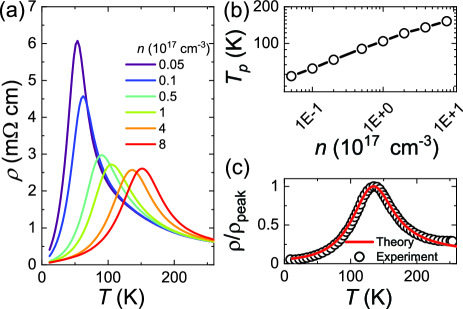
Figure 2: (a) The zero-field resistivity $\rho$ as a function of temperature for several carrier density $n$. (b) The peak temperature $T_{p}$ as a function of the carrier density. (c) The comparison of the experimental data and theoretical prediction by using the same parameters as Fig. 1. The experimental data are extracted from Fig. 1(d) in Ref. ((zhang2017electronic, )). Both resistivity curves have been normalized to their maximum values $\rho_{\mathrm{peak}}$.

The resistivity anomaly

With the phonon-induced self-energy in hand, we are ready to present the electrical resistivity as a function of temperature by means of the linear response theory (Mahan-book, ; Note-on-SM, ). At finite temperatures, the conductivities and thermoelectric coefficients are contributed from both the electron-like and hole-like bands after the phonon-induced renormalization. The two contributions are weighted by the negative energy derivative of the Fermi-Dirac function, whose value is nearly zero except for energies within a narrow window of $k_{B}T$ near the chemical potential $\mu$. Figure 2(a) reproduces the resistivity peak at several initial chemical potentials $\mu$, or equivalently carrier densities at $T=0$. For the initial $\mu(T=0)$ ($>0$) locating in the conduction band, as it moves down to the valance band with increasing temperature, it will inevitably sweep over the band gap. When $T=T_{p}$, the effective chemical potential lies around the middle of the effective band gap $\mu(T=T_{p})\simeq 0$ and the resistivity reaches the maximum. As the $n$-type carrier concentration is decreased, the resistivity peak will move to the lower temperature with the higher magnitude. The peak temperature as a function of the carrier density is plotted in Fig. 2(b). For a lower carrier concentration, the chemical potential reaches the middle of the band gap with a lower temperature. The height of the resistivity peak is determined by the ratio $\bar{m}(T_{p})/(k_{B}T_{p})$. With increasing the ratio, the peak height increases drastically, and becomes divergent if $\bar{m}(T_{p})\gg k_{B}T_{p}$. It explains why in some experiments with extreme low carrier concentration no resistivity peak is observed (liang2018anomalous, ; mutch2019evidence, ), which can be regarded as the situation of $T_{p}\sim 0$. Thus the sweeping chemical potential over the band gap of Dirac fermions gives rise to the resistivity anomaly at finite temperatures. We use the model parameters in Fig. 1 to calculate the resistivity, which is in a good agreement with the experimental data as shown in Fig. 2(c).The slight deviation at the high temperature might be caused by neglecting the contributions from the optical modes of phonons.

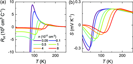
Figure 3: (a) The Hall coefficient $R_{H}$ and (b) the Seebeck coefficient $S$ as functions of temperature several carrier density $n$.

Sign change of the Hall and Seebeck coefficients

The resistivity anomaly is always accompanied with the sign change of the Hall and Seebeck coefficients around the transition temperature(jones1982thermoelectric, ; chi2017lifshitz, ; zhang2020observation, ; tang2019three, ; Miller2018polycrystalline, ; Niemann2019magnetothermoelectric, ), which can be reproduced in the present theory. As shown in Fig. 3(a), for a positive $\mu(T=0)$ or $n$-type carriers , with increasing the temperature, the Hall coefficient ($R_{H}=\partial\rho_{xy}/\partial B|_{B=0}$) first maintains its value ($1/en$) at low temperature, decreases down until reaching the minimum. Then $R_{H}$ changes from the negative to positive sign at some temperature and continues to decrease down to nearly zero at high temperatures. The sign change of $R_{H}$ indicates the electron-dominated transport is transformed into the hole-dominated as the chemical potential moves from the conduction band to valence band. As the carrier concentration decreases, the Hall coefficient crosses $0$ at a lower temperature with a larger maximum. In Fig. 3(b), the Seebeck coefficient $S_{xx}$ also reveals a systematic shift in temperature as the carrier density increases. For each curve with fixed carrier density, $S_{xx}$ displays similar nonmonotonic temperature dependence as $R_{H}$, except that $S_{xx}$ starts from absolute zero and exhibits a relative large positive ($p$-type) Seebeck coefficient at high temperatures. At low temperatures, the chemical potential lies deep in the bulk band, the Mott formula relates the thermoelectric conductivity with the derivative of the electrical conductivity for the thermopower $S_{xx}=\frac{\pi^{2}k_{B}^{2}T}{3e}\frac{d\sigma(\omega)/d\omega}{\sigma(\omega)}|_{\omega=\mu}$ (Mott1969observation, ) with $\sigma(\omega)$ is the energy-dependent conductivity. The conductivity $\sigma(\omega)$ is proportional to the square of the group velocity. Hence, as chemical potential locates in conduction band, $S_{xx}$ is negative ($n$-type) and decreases with increasing temperature. $S_{xx}$ attains its largest value when $n$ is tiny but nonvanishing, and varies rapidly with the temperature around $T_{p}$. (Nolas, ). $T_{p}$ decreases with the reduction of the $n$-type carrier concentration at zero temperature qualitatively agrees with previous measurements for single crystals with different carrier concentrations (chi2017lifshitz, ). Near $T=T_{p}$ and if the band gap $\bar{m}(T_{p})$ is comparably smaller than the thermal energy $k_{B}T_{p}$, either $R_{H}$ or $S_{xx}$ is linear in temperature and the system enters a nearly neutral state of Dirac polarons due to the strong thermal activation.

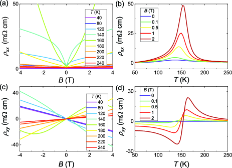
Figure 4: The magnetic field dependence of (a) the transverse magnetoresistance $\rho_{xx}$ and (c) the Hall resistivity $\rho_{xy}$ for different temperatures. The temperature dependence of (b) $\rho_{xx}$ and (d) $\rho_{xy}$for different magnetic fields.

Magnetotransport in nearly neutral state of Dirac polarons

The presence of an external magnetic field reveals the exotic behaviors of magnetoresistivity near the transition temperature (tritt1999enhancement, ; li2016chiral, ; tang2019three, ; Zhao2017anomalous, ; lv2018tunalbe, ; Niemann2019magnetothermoelectric, ). Without loss of generality we assume the magnetic field $B$is along the $z$ direction. As shown in Fig. 4(a), the transverse magnetoresistivity $\rho_{xx}(B)$ displays significantly different behaviors for temperature above and below $T_{p}$. Below 120K, a narrow dip is observed around zero magnetic field and above 200K, $\rho_{xx}$ shows a quadratic field dependence. As approaching the peak temperature, $\rho_{xx}$ becomes large and nonsaturating. We plot the resistivity as a function of temperature for different magnetic fields. As shown in Fig. 4(b), $\rho_{xx}(B)$ displays striking resistivity peaks when the temperature crosses the region of the neutral state of Dirac polarons. The peak is strongly enhanced with increasing magnetic field, and even becomes nonsaturated. Its position is observed to shift slightly to a higher temperature with the field increasing, i.e. $T_{p}$ is a function of $B$. This effect has been reported experimentally in Ref. (li2016chiral, ; tang2019three, ). The appearance of giant and nonsaturated transverse magnetoresistivity can be viewed as the electrical signature of the neutral state of Dirac polarons. As shown in Fig. 4(c), the slope of the Hall resistivity $\rho_{xy}$ is negative, indicating a electron-dominated charge transport. As the temperature increases, the nonlinearity of $\rho_{xy}$ becomes more apparent. In the intermediate temperature ($120\sim 180$K) around $T_{p}$, due to the formation of the nearly neutral state of Dirac polarons, the slope of the Hall resistivity changes from positive (hole type) at low magnetic field to negative (electron type) at high field, showing a zigzag shaped profile. At high temperature (above 200K), the hole carrier dominates the charge transport thus the slope of $\rho_{xy}$ become positive. The effect of an applied magnetic field on $\rho_{xy}$ as a function of temperature is shown in Fig. 4(d). There is a systematic shift to the higher temperatures with increasing field. The calculated $\rho_{xx}$ and $\rho_{xy}$ as functions of either $T$ or $B$ are in an excellent agreement with the experimental measurements in $\text{ZrTe}_{5}$ and $\mathrm{HfTe}_{5}$ (Zhao2017anomalous, ; tang2019three, ; Niemann2019magnetothermoelectric, ; lv2018tunalbe, ). Lastly, we want to point out the differences between the present theory and the two-carrier model for magnetoresistance (Pippard1989, ). The two-carrier model commonly requires that the Fermi surface is composed of both electron and hole pockets and predicts a quadratical magnetoresistance, while the present theory only involves a single Dirac band crossing the Fermi surface and the multi-carrier transport is attributted to thermal excitation over a wide range of temperature.

Discussion

From an experimental standpoint, a temperature-dependent effective carrier density can be deduced from the Hall measurement. The shift of the chemical potential or effective carrier density with the variation of temperature is the key issue to the resistivity anomaly. With no absorption or desorption process through extrinsic doping, the temperature dependent variation of effective density of charge carriers seems to violate the conservation law of the total charge. However, the relative contribution from each band of carriers to the total Hall effect also depends on its ability to respond to the applied magnetic field such as velocity and mobility. In Dirac materials with extreme low carrier density and tiny band gap, the strong particle-hole asymmetry will induce a significant temperature variation of the chemical potential, even shifts from conduction band to valence band. Consequently, the effective carrier density also displays strong temperature dependence.

We thank Li-Yuan Zhang, Nan-Lin Wang and Chen-Jie Wang for helpful discussions. This work was supported by the Research Grants Council, University Grants Committee, Hong Kong under Grant No. 17301717.

Supplementary Materials for “Dirac Polarons and Resistivity Anomaly in $\mathrm{ZrTe}_{5}$ and $\mathrm{HfTe}_{5}$”

I The Model Hamiltonian for Anisotropic Dirac Materials

For a three-dimensional quantum spin Hall system or topological insulator, three are four $Z_{2}$ invariants to characterize 16 distinct phases, in sharp contrast with two-dimensional case that only a single $Z_{2}$ topological invariant governs the effect (fu2007topological-1). For a cubic lattice, three are 8 time reversal invariant momenta (TRIM) expressed in terms of primitive reciprocal lattice vectors are $\Gamma_{i=(n_{1}n_{2}n_{3})}=(n_{1}\mathbf{b}_{1}+n_{2}\mathbf{b}_{2}+n_{3}\mathbf{b}_{3})/2$ with $n_{j}=0,1$. The four $Z_{2}$ topological invariants $(\nu_{0};\nu_{1}\nu_{2}\nu_{3})$ are defined as

$$(-1)^{\nu_{0}} =\prod_{n_{j}=0,1}\delta_{n_{1},n_{2},n_{3}},$$

$$(-1)^{\nu_{i=1,2,3}} =\prod_{n_{j\neq i}=0,1;n_{i}=1}\delta_{n_{1},n_{2},n_{3}}.$$

Generally, the calculation of $\delta_{i}$ requires a gauge in which the wavefunctions are globally continuous, but in practice it is not simple. When the system possesses the inversion symmetry, the problem of identifying the $Z_{2}$ invariants is greatly simplified. In this case, we only need to evaluate the expectation value of the parity operator at the eight TRIMs which are the same for the two Kramers degenerate states and

$$\delta_{i}=\prod_{m=1}^{N}\xi_{2m}(\Gamma_{i})$$

where $\xi_{2m}(\Gamma_{i})=\pm 1$ is the parity eigenvalue of the degenerate states. The analytic expression for $\delta_{i}$ can be obtained,

$$\delta_{i}=\frac{m(\Gamma_{i})}{|m(\Gamma_{i})|}.$$

To identify the topology of the system, we need to take into account the entire Brillouin zone, carefully examining the parity eigenvalues at eight time-reversal invariant momenta. Our theory is based on $\boldsymbol{k}\cdot\boldsymbol{p}$ theory which is only valid around the Fermi level, NOT in the whole Brillouin zone. In order to clarify the topology of the system, we use the widely employed strategy to extend the low-energy continuous model to a tight-binding model on a cubic lattice by replacing $k_{i}$ to $\sin k_{i}$ and $k_{i}^{2}$ to $2(1-\cos k_{i})$. Then the mass term reads as $m(\mathbf{k})=m-2b_{x}(1-\cos k_{x})-2b_{y}(1-\cos k_{y})-2b_{z}(1-\cos k_{z})$. Now we consider an anisotropic modified Dirac model with $b_{x}=b_{y}>0,b_{z}<0$ and $|b_{x}|>|b_{z}|$ because of the high anisotropic band structure of $\mathrm{ZrTe}_{5}$ and $\mathrm{HfTe}_{5}$. For simplicity, we assume it is nearly isotropic in the a-c plane. To ensure the lowest energy electronic states for the entire spectrum is located at the $\Gamma$ point, we can choose a small $|m|$. In this case, the four $Z_{2}$ invariants can be obtained as,

$$(-1)^{\nu_{0}} =sgn(m),$$

$$(-1)^{\nu_{1}} =1,$$

$$(-1)^{\nu_{2}} =1,$$

$$(-1)^{\nu_{3}} =-1.$$

Thus,the topological nature of this anisotropic Dirac model is controlled by the sign of parameter $m$ such that an strong TI phase with $Z_{2}$ indices $(\nu_{0};\nu_{1}\nu_{2}\nu_{3})=(1,001)$ appears when $m<0$, while the regime of $m>0$ falls into a weak TI phase with $(\nu_{0};\nu_{1}\nu_{2}\nu_{3})=(0,001)$. This result is consistent with the first principles calculation in Ref.((weng2014transition-1)).

The transport properties discussed in this work and its relevant physics are determined mainly by the electrons near the Fermi surface. The low-energy effective Dirac Hamiltonian successfully captures important features of the band structure around the Fermi energy and the main physics we are interested in. In the ARPES experiment, no surface states can be observed within the gap in the the a-c plane (with the layers stacking along the b axis) of $\mathrm{ZrTe}_{5}$ , with lowering the temperature the energy gap tends to decrease and no topological phase transition over the entire temperature range (zhang2017electronic-1). To be consistent with the experimental observations, we adopt an anisotropic Dirac model up to the quadratic term of the momentum which describes the low-energy physics for the weak topological insulator

$$\mathcal{H}_{Dirac}=(d(\mathbf{q})-\mu)I+\sum_{i=x,y,z}\hbar v_{i}p_{i}\alpha_{i}+m(\mathbf{p})\beta,$$

with the particle-hole asymmetry term $d(\mathbf{q})=\sum_{i=x,y,z}d_{i}p_{i}^{2}$ and the mass term as $m(\mathbf{p})=m-\sum_{i=x,y,z}b_{i}p_{i}^{2}$. For the convenience in explicit calculation, we use the parameters as $v_{x}\simeq v_{y}=v_{\perp}$ $b_{x}\simeq b_{y}=b_{\perp}$, $b_{z}=0$, $d_{x}\simeq d_{y}=d_{\perp}$and $d_{z}=0$, which can be viewed as the minimal model for the band structure near the $\Gamma$ point of an anisotropic weak topological insulator.

II The Model for Electron-Phonon Interactions

The Hamiltonian for lattice vibration in the harmonic approximation can be expressed as

$$\mathcal{H}_{ph}=\sum_{\mathbf{q},\lambda}\hbar\omega_{\mathbf{q},\lambda}\left(a_{\mathbf{q}\lambda}^{\dagger}a_{\mathbf{q}\lambda}+\frac{1}{2}\right),$$ (4)

where $\omega_{\mathbf{q},\lambda}$ denotes the frequency of the $\lambda$-th normal mode of wavevector $\mathbf{q}$. The DFT-calculations demonstrate that the phonon energy ranges from $0$ to $28.9$ meV, which corresponds an upper bound of the phonon frequency $\omega/2\pi\approx 7\,\mathrm{THz}$ (zhu2018record, ). The velocities for the acoustic phonons at $\Gamma$ point along $a,b,c$ axis are $2217$, $494$, and $2185\mathrm{ms^{-1}}$ (zhu2018record, ), respectively. The acoustic phonon velocity along the $b$ axis is significantly smaller than those along the $a,c$ axis. $\mathrm{Te}$ atoms give the dominate contribution to the acoustic phonons as well as the low-energy optical modes $(<5.5\mathrm{THz})$ and due to the large stoichiometric ratio and heavier atomic mass. Among total $36$ phonon bands ($12$ atoms in the primitive unite cell), there are $3$ acoustic modes, $13$ inversion symmetry breaking infrared-active optical modes, $18$ inversion symmetry preserving Raman-active optical modes, and $2$ optical modes are optically inactive. Further considering the constraint of the space-group symmetry of $\mathrm{ZrTe}_{5}$, there are $6$ full crystalline symmetry protecting $A_{g}$ Raman modes (Aryal2020topological, ). The variation of the atomic displacement vectors for these modes will drive the system into various topological phases. A Dirac topology surface separating the strong topological insulator phase and the weak topological insulator phase thus can be identified in the 6-dimensional space spanned by these symmetry allowed Raman modes. The slight change in the lattice parameters can be viewed as the superposition of the phonon modes and corresponds to a single point in the formed multi-dimensional space. Thus, the different sample growth conditions or some other external perturbations such as strain and temperature may allocate the system in distinct topological phases.

It is believed that acoustic phonons play a dominant role in modifying the electronic properties and the carrier scattering at low temperature. We consider that the EPI part $\mathcal{H}_{ep}$ is dominantly contributed by longitudinal acoustic phonons, which can be expressed as

$$\mathcal{H}_{ep}=\sum_{\mathbf{q},\mathbf{k}}M_{\mathbf{q}}(a_{\mathbf{q}}+a_{-\mathbf{q}}^{\dagger})\psi_{\mathbf{k}+\mathbf{q}}^{\dagger}\psi_{\mathbf{k}}$$ (5)

with the EPI strength as $M_{\mathbf{q}}=\sqrt{\hbar\mathbf{q}^{2}\Xi^{2}/(2V\varrho\omega_{\mathbf{q}})}$ where $\varrho=6.366\times 10^{3}\mathrm{kgm^{-3}}$ is the atomic mass density for $\mathrm{ZrTe_{5}}$, $\Xi=6\mathrm{eV}$ is the acoustic deformation potential and $\omega_{\mathbf{q}}=c_{s}q$ is the acoustic phonon frequency with the sound velocity chosen as $c_{s}=3040\,\mathrm{m}s^{-1}$, $V=NV_{0}$ is the total volume with the unit cell volume for $\mathrm{ZrTe}_{5}$ as $V_{0}\approx 400\mathring{\mathrm{A}}^{3}$ (zhang2020observation, ). Note that electron-phonon scattering of the deformation potential type conserves spin and pseudospin degrees of freedom. Here, for simplicity, we adopt the isotropic model for $\mathrm{ZrTe}_{5}$. It is believed that the anisotropy will only cause some quantitative, not quantitative correction to the main results.

III The phonon-induced self-energy

To explore the EPI effect, we treat $\mathcal{H}_{ep}$ as a perturbation to either electrons or phonons. It will give rise to the quasiparticle properties of the renormalized electrons and phonons. By definition, the imaginary-time Green’s functions for fermionic quasiparticle are

$$G(\mathbf{p},ip_{n})=-\int_{0}^{1/k_{B}T}d\tau e^{ip_{n}\tau}\langle T_{\tau}\psi_{\mathbf{p}}(\tau)\psi_{\mathbf{p}}^{\dagger}(0)\rangle$$ (6)

and for bosonic quasiparticle

$$D(\mathbf{q},iq_{n})=-\int_{0}^{1/k_{B}T}d\tau e^{iq_{n}\tau}\langle T_{\tau}(a_{\mathbf{q}}(\tau)+a_{-\mathbf{q}}^{\dagger}(\tau))(a_{-\mathbf{q}}(0)+a_{\mathbf{q}}^{\dagger}(0))\rangle$$ (7)

where $p_{n}=(2n+1)\pi k_{B}T$ and $q_{m}=2m\pi k_{B}T$ denote the fermionic and bosonic Matsubara frequencies, respectively, with $n,m$ being integer numbers and $k_{B}$ is the Boltzmann constant. In the interacting system, the electronic structure is characterized by the renormalized finite-temperature Green’s function $G(\mathbf{p},ip_{n})=[G^{(0)}(\mathbf{p},ip_{n})^{-1}+\Sigma(\mathbf{p},ip_{n})]^{-1}$ (Mahan-book, ). The bare Green’s function for the unperturbed Dirac Hamiltonian is

$$G^{(0)}(\mathbf{p},ip_{n})=\sum_{\zeta=\pm}\frac{\mathcal{P}_{\zeta}(\mathbf{p})}{ip_{n}-\xi_{\mathbf{p}}^{\zeta}},$$ (8)

with the projection operators for the two bands are define as

$$\mathcal{P}_{\zeta}(\mathbf{p})=\frac{1}{2}\left\{1+\left[\sum_{i}\hbar v_{i}p_{i}\alpha_{i}+m_{\mathbf{p}}\beta\right]]/\epsilon_{\mathbf{p}}^{\zeta}\right\}$$ (9)

and the eigenvalues $\xi_{\mathbf{p}}^{\zeta}=d(\mathbf{p})-\mu+\zeta\epsilon_{\mathbf{p}}$ with $\epsilon_{\mathbf{p}}=\sqrt{\sum_{i=x,y,z}\hbar^{2}v_{i}^{2}p_{i}^{2}+m^{2}(\mathbf{p})}$ are doubly degenerate for the conduction ($\zeta=+$) and valance ($\zeta=-$) bands which are measured with respect to the chemical potential. In Dirac materials, the renormalization of the electron-phonon vertex and higher order corrections to self-energy scale as the ratio of sound to Fermi velocity $c_{s}/v_{F}$, which is a small quantity in our problem. Thus, we only consider the lowest-order electron self-energy arising from the virtual exchange of one phonon, which can be expressed as (Migdal-58jetp, )

$$\Sigma_{ep}(\mathbf{p},ip_{n}) =-k_{B}T\sum_{iq_{m},\mathbf{q}}|M_{\mathbf{q}}|^{2}D^{(0)}(\mathbf{q},iq_{m})G^{(0)}(\mathbf{p}+\mathbf{q},ip_{n}+iq_{m})$$ (10)

with the bare phonon Green’s functions $D^{(0)}(\mathbf{q},iq_{m})=\frac{-2\omega_{\mathbf{q}}}{q_{m}^{2}+\omega_{\mathbf{q}}^{2}}$. After performing the Matsubara summation over frequencies $\omega_{n}$, one obtains

$$\Sigma_{ep}(\mathbf{p},ip_{n})=\sum_{\zeta}\sum_{\mathbf{q}}|M_{\mathbf{q}}|^{2}\mathcal{P}_{\zeta}(\mathbf{p}+\mathbf{q})\left(\frac{n_{B}(\omega_{\mathbf{q}})+n_{F}(\xi_{\mathbf{p}+\mathbf{q}}^{\zeta})}{ip_{n}+\omega_{\mathbf{q}}-\xi_{\mathbf{p}+\mathbf{q}}^{\zeta}}+\frac{n_{B}(\omega_{\mathbf{q}})+1-n_{F}(\xi_{\mathbf{p}+\mathbf{q}}^{\zeta})}{ip_{n}-\omega_{\mathbf{q}}-\xi_{\mathbf{p}+\mathbf{q}}^{\zeta}}\right).$$ (11)

The self-energy depends on temperature via the Fermi-Dirac distribution function $n_{F}(\varepsilon)=(e^{\varepsilon/k_{B}T}+1)^{-1}$and Bose-Einstein distribution function $n_{B}(\varepsilon)=(e^{\varepsilon/k_{B}T}-1)^{-1}$, respectively. Due to the EPI, for the state $|\zeta s\mathbf{p}\rangle$ with momentum $\mathbf{p}$ of the conduction band $\zeta=+$, it can scatter virtually to the state $\xi_{\mathbf{p}+\mathbf{q}}^{\zeta}+\omega_{\mathbf{q}}$ with higher energy under simultaneous absorption of a phonon, or to the state $\xi_{\mathbf{p}+\mathbf{q}}^{\zeta}-\omega_{\mathbf{q}}$ with lower energy under simultaneous emission of a phonon, respectively. The integral over the momentum can be evaluated numerically by noticing that the integrands depend only on the angle between momentum $\mathbf{p}$ and $\mathbf{q}$. To discuss the quasiparticle renormalization, the retarded Green’s function $G^{R}(\mathbf{p},\epsilon)$ and self-energy $\Sigma^{R}(\mathbf{p},\epsilon)$ can be obtained by analytic continuation to the real axis via $ip_{n}\to\epsilon+i\delta$ with an infinitesimal positive $\delta$.

In some limiting regimes, the analytic expressions for these quantities are available. At low temperatures $T\ll\Theta_{D}$, where $\Theta_{D}=\hbar c_{s}\Lambda/k_{B}$ is the Debye temperature with $\Lambda\sim\pi/a$ the high momentum cutoff (in this work we use $\Lambda=6.28\mathrm{nm}^{-1}$ which corresponds a Debye temperature $\Theta_{D}\sim 150$K (zhang2017electronic, )), the Bose-Einstein distribution function falls off exponentially for $\hbar\omega_{\mathbf{q}}>k_{B}T$ and only the lower energy acoustic phonons modes with long wavelength are active, the imaginary part of self-energy follows a cubic temperature dependence and the real part of self-energy saturate at a constant. Thus both the imaginary and real part of the self-energy are linear in $T$. In high and low temperature limits, the explicit expressions for imaginary part of $\Sigma_{I}^{R}$,

$$\mathrm{Im}\Sigma_{\zeta}^{R}(\mathbf{p},\epsilon+i\delta) =-\frac{\pi}{2}\sum_{\zeta^{\prime}}\sum_{\mathbf{q}}M_{\mathbf{q}}^{2}\mathrm{Tr}[\mathcal{P}_{\zeta}(\mathbf{p})\mathcal{P}_{\zeta^{\prime}}(\mathbf{p}+\mathbf{q})]\Bigg{\{}\left[n_{B}(\omega_{\mathbf{q}})+n_{F}(\xi_{\mathbf{p}+\mathbf{q}}^{\zeta^{\prime}})\right]\delta(\epsilon+\omega_{\mathbf{q}}-\xi_{\mathbf{p}+\mathbf{q}}^{\zeta^{\prime}})$$

$$+\left[n_{B}(\omega_{\mathbf{q}})+1-n_{F}(\xi_{\mathbf{p}+\mathbf{q}}^{\zeta^{\prime}})\right]\delta(\epsilon-\omega_{\mathbf{q}}-\xi_{\mathbf{p}+\mathbf{q}}^{\zeta^{\prime}})\Bigg{\}}$$

Since the phonon energy is much smaller than the bulk band gap, the delta function vanishes unless $\zeta=\zeta^{\prime}$. We further set $\epsilon=\xi_{\mathbf{p}}^{\zeta}$, which is good approximation when it is smaller than the chemical potential. For high temperature $T\gg\Theta_{D}$, the Bose function takes the classical limit $n_{B}(\omega_{\mathbf{q}})\approx k_{B}T/(\hbar\omega_{\mathbf{q}})\gg 1$, the energy difference between two electron energies for the typical momenta is much larger than the phonon energies $\omega_{\mathbf{q}}$ thus can be neglected in the delta functions. With these simplifications, we have

$$\mathrm{Im}\Sigma_{\zeta}^{R}(\mathbf{p},\xi_{\mathbf{p}}^{\zeta}) =-\frac{\pi}{2}\frac{\Xi^{2}k_{B}T}{\varrho c_{s}^{2}}\frac{1}{V}\sum_{\mathbf{p}^{\prime}}\mathrm{Tr}[\mathcal{P}_{\zeta}(\mathbf{p})\mathcal{P}_{\zeta}(\mathbf{p}^{\prime})]\delta(\xi_{\mathbf{p}}^{\zeta}-\xi_{\mathbf{p}^{\prime}}^{\zeta}).$$

In this situation, the phonons can be viewed as the “thermal static disorder” from the lattice, and the effective disorder strength is proportional to $\Xi^{2}k_{B}T/(\varrho c_{s}^{2})$. By introducing the density of states per band at the Fermi level $\nu(\mu)=\frac{1}{V}\sum_{\zeta}\sum_{\mathbf{p}}\delta(\xi_{\mathbf{p}}^{\zeta})$ and the Fermi-surface average of $A_{\mathbf{k}}$,

$$\langle A\rangle_{FS}=\left[\sum_{\xi}\sum_{\mathbf{k}}A_{\mathbf{k}}\delta(\xi_{\mathbf{p}}^{\zeta})\right]\Big{/}\left[\sum_{\xi}\sum_{\mathbf{k}}\delta(\xi_{\mathbf{p}}^{\zeta})\right],$$

the imaginary part of the self-energy averaged over Fermi surface at high temperature can be expressed as,

$$\langle\mathrm{Im}\Sigma_{\zeta}^{R}(\mathbf{p},\xi_{\mathbf{p}}^{\zeta})\rangle_{FS}=-\frac{\pi}{2}\frac{\Xi^{2}k_{B}T}{\varrho c_{s}^{2}}\nu(\mu)\left[1+\langle\eta(\mathbf{p})\rangle_{FS}^{2}\right],$$

with $\eta(\mathbf{p})=\frac{m_{\mathbf{p}}}{\epsilon_{\mathbf{p}}}$ the orbital polarization.

For low temperature $T\ll\Theta_{D}$, typical phonons have energy $\omega_{\mathbf{q}}\sim k_{B}T$ and momenta $q\sim k_{B}T/\hbar c_{s}\ll\Theta_{D}/\hbar c_{s}\sim k_{F}$, the argument of delta-function thus can be expanded as $\xi_{\mathbf{p}}^{\zeta}\pm\omega_{\mathbf{q}}-\xi_{\mathbf{p}+\mathbf{q}}^{\zeta}\approx\pm\omega_{\mathbf{q}}-\hbar\mathbf{v}_{\mathbf{p}}^{\zeta}\cdot\mathbf{q}$ with $\mathbf{v}_{\mathbf{p}}^{\zeta}=\frac{\partial\xi_{\mathbf{p}}^{\zeta}}{\hbar\partial\mathbf{p}}$ is the group velocity. After taking average over Fermi surface, we have

$$\langle\mathrm{Im}\Sigma_{\zeta}^{R}(\mathbf{p},\xi_{\mathbf{p}}^{\zeta})\rangle_{FS} \approx-\frac{\pi}{V}\sum_{\mathbf{p}}\sum_{\mathbf{q}}M_{\mathbf{q}}^{2}\left[n_{B}(\omega_{\mathbf{q}})+n_{F}(\omega_{\mathbf{q}})\right]\left[\delta(\omega_{\mathbf{q}}+\hbar\mathbf{v}_{\mathbf{p}}^{\zeta}\cdot\mathbf{q})+\delta(\omega_{\mathbf{q}}-\hbar\mathbf{v}_{\mathbf{p}}^{\zeta}\cdot\mathbf{q})\right]\delta(\xi_{\mathbf{p}}^{\zeta})$$

$$\approx-\pi\sum_{\mathbf{q}}M_{\mathbf{q}}^{2}\left[n_{B}(\omega_{\mathbf{q}})+n_{F}(\omega_{\mathbf{q}})\right]\left[\delta(\omega_{\mathbf{q}}+\hbar\langle|\mathbf{v}_{\mathbf{p}}^{\zeta}|\rangle_{FS}|\mathbf{q}|\cos\theta)+\delta(\omega_{\mathbf{q}}-\hbar\langle|\mathbf{v}_{\mathbf{p}}^{\zeta}|\rangle_{FS}|\mathbf{q}|\cos\theta)\right]$$

$$=-\frac{\hbar c_{s}\Xi^{2}}{4\pi\varrho c_{s}^{2}}\left(\frac{k_{B}T}{\hbar c_{s}}\right)^{3}\frac{1}{\hbar\langle|\mathbf{v}_{\mathbf{p}}^{\zeta}|\rangle_{FS}}\int_{0}^{\infty}dxx^{2}\left[\frac{1}{e^{x}+1}+\frac{1}{e^{x}-1}\right]$$

$$=-\frac{7\zeta(3)}{8\pi}\frac{\hbar\Xi^{2}}{\varrho c_{s}}\left(\frac{k_{B}T}{\hbar c_{s}}\right)^{3}\frac{1}{\hbar\langle|\mathbf{v}_{\mathbf{p}}^{\zeta}|\rangle_{FS}}.$$

The final results for imaginary part of self-energy are collected as,

$$\langle\mathrm{Im}\Sigma_{\zeta}^{R}(\mathbf{p},\xi_{\mathbf{p}}^{\zeta})\rangle_{FS} \approx\begin{cases}-\frac{7\zeta(3)}{8\pi}\frac{\hbar\Xi^{2}}{\varrho c_{s}}\left(\frac{k_{B}T}{\hbar c_{s}}\right)^{3}\frac{1}{\hbar\langle|\mathbf{v}_{\mathbf{p}}^{\zeta}|\rangle_{FS}},&T\ll\Theta_{D};\\ -\frac{\pi}{2}\frac{\hbar\Xi^{2}}{\varrho c_{s}}\frac{k_{B}T}{\hbar c_{s}}\nu_{\zeta}(\xi_{\mathbf{p}}^{\zeta})\left[1+\langle\eta(\mathbf{p})\rangle_{FS}^{2}\right],&T\gg\Theta_{D}.\end{cases}$$ (12)

Now we calculate the real part of the self-energy. We concentrate on the results at $\mathbf{p}=0$ which describe the energy renormalization for the states at the band edge. Noticing that the dominant contribution comes from the large momentum, it is a good approximation to further let $\epsilon=0$. With these assumptions, the real part of self-energies for the chemical potential, the Dirac mass and the velocity can be calculated through,

$$\mathrm{Re}\Sigma_{I}(\mathbf{0},0) =\frac{1}{2}\sum_{\chi}\sum_{\mathbf{q}}|M_{\mathbf{q}}|^{2}\left(\frac{n_{B}(\omega_{\mathbf{q}})+n_{F}(\xi_{\mathbf{q}}^{\chi})}{\omega_{\mathbf{q}}-\xi_{\mathbf{q}}^{\chi}}+\frac{n_{B}(\omega_{\mathbf{q}})+1-n_{F}(\xi_{\mathbf{q}}^{\chi})}{-\omega_{\mathbf{q}}-\xi_{\mathbf{q}}^{\chi}}\right),$$

$$\mathrm{Re}\Sigma_{\beta}(\mathbf{0},0) =\frac{1}{2}\sum_{\chi}\sum_{\mathbf{q}}|M_{\mathbf{q}}|^{2}\chi\eta(\mathbf{q})\left(\frac{n_{B}(\omega_{\mathbf{q}})+n_{F}(\xi_{\mathbf{q}}^{\chi})}{\omega_{\mathbf{q}}-\xi_{\mathbf{q}}^{\chi}}+\frac{n_{B}(\omega_{\mathbf{q}})+1-n_{F}(\xi_{\mathbf{q}}^{\chi})}{-\omega_{\mathbf{q}}-\xi_{\mathbf{q}}^{\chi}}\right),$$

$$\lambda_{\alpha} =\frac{1}{2}\sum_{\chi}\sum_{\mathbf{q}}|M_{\mathbf{q}}|^{2}\frac{1}{\epsilon_{\mathbf{q}}^{\chi}}\left(\frac{n_{B}(\omega_{\mathbf{q}})+n_{F}(\xi_{\mathbf{q}}^{\chi})}{\omega_{\mathbf{q}}-\xi_{\mathbf{q}}^{\chi}}+\frac{n_{B}(\omega_{\mathbf{q}})+1-n_{F}(\xi_{\mathbf{q}}^{\chi})}{-\omega_{\mathbf{q}}-\xi_{\mathbf{q}}^{\chi}}\right).$$

In evaluating the real part of self-energy, the phonon energy $\omega_{\mathbf{q}}$ in the denominator is less important and can be neglected. The two terms in the parentheses has the same denominator, then the Fermi factors cancel when they are added. At low temperature, $n_{B}(\omega_{\mathbf{q}})\approx 0$, and at high temperature, $n_{B}(\omega_{\mathbf{q}})\approx k_{B}T/\omega_{\mathbf{q}}$. After introducing some constants independent of temperature,

$$\mathcal{C}_{\beta}^{H} =\frac{\hbar c_{s}\Lambda}{\Lambda^{3}}\int_{|\mathbf{q}|<\Lambda}\frac{d^{3}\mathbf{q}}{(2\pi)^{3}}\frac{m(\mathbf{q})}{(d(\mathbf{q})-\mu)^{2}-\epsilon_{\mathbf{q}}^{2}};\mathcal{C}_{\beta}^{L}=\frac{1}{2\Lambda^{3}}\int_{|\mathbf{q}|<\Lambda}\frac{d^{3}\mathbf{q}}{(2\pi)^{3}}\frac{\hbar c_{s}qm(\mathbf{q})}{(d(\mathbf{q})-\mu)^{2}-\epsilon_{\mathbf{q}}^{2}};$$

$$\mathcal{C}_{I}^{H} =\frac{\hbar c_{s}\Lambda}{\Lambda^{3}}\int_{|\mathbf{q}|<\Lambda}\frac{d^{3}\mathbf{q}}{(2\pi)^{3}}\frac{\mu-d(\mathbf{q})}{(d(\mathbf{q})-\mu)^{2}-\epsilon_{\mathbf{q}}^{2}};\mathcal{C}_{I}^{L}=\frac{1}{2\Lambda^{3}}\int_{|\mathbf{q}|<\Lambda}\frac{d^{3}\mathbf{q}}{(2\pi)^{3}}\frac{\hbar c_{s}q(\mu-d(\mathbf{q}))}{(d(\mathbf{q})-\mu)^{2}-\epsilon_{\mathbf{q}}^{2}};$$

$$\mathcal{C}_{\alpha}^{H} =\frac{\hbar c_{s}\Lambda}{\Lambda^{3}}\int_{|\mathbf{q}|<\Lambda}\frac{d^{3}\mathbf{q}}{(2\pi)^{3}}\frac{1}{(d(\mathbf{q})-\mu)^{2}-\epsilon_{\mathbf{q}}^{2}};\mathcal{C}_{\alpha}^{L}=\frac{1}{2\Lambda^{3}}\int_{|\mathbf{q}|<\Lambda}\frac{d^{3}\mathbf{q}}{(2\pi)^{3}}\frac{\hbar c_{s}q}{(d(\mathbf{q})-\mu)^{2}-\epsilon_{\mathbf{q}}^{2}}.$$

The real part of $\Sigma_{I}^{R}$ and $\Sigma_{\beta}^{R}$ can be expressed as

$$\mathrm{Re}\Sigma_{I,\beta}^{R}(\mathbf{0},0)=\frac{\Xi^{2}\Lambda^{3}}{\varrho c_{s}^{2}}\begin{cases}\mathcal{C}_{I,\beta}^{L},&T\ll\Theta_{D};\\ \frac{k_{B}T}{\hbar c_{s}\Lambda}\mathcal{C}_{I,\beta}^{H},&T\gg\Theta_{D}.\end{cases}$$ (13)

Thus the effective Dirac mass due to EPI can be obtained as $\bar{m}=m+\mathrm{Re}\Sigma_{\beta}(\mathbf{0},0)$, which exhibits strong temperature dependence. Since the EPI strength is momentum-dependent, the velocity renormalization $\lambda_{\alpha}(\mathbf{p},\epsilon)$ do not vanish. In the high and low temperature limits, the renormalization factor can be obtained as,

$$\lambda_{\alpha}=\frac{\Xi^{2}\Lambda^{3}}{\varrho c_{s}^{2}}\begin{cases}\mathcal{C}_{\alpha}^{L},&T\ll\Theta_{D}\\ \frac{k_{B}T}{\hbar c_{s}\Lambda}\mathcal{C}_{\alpha}^{H},&T\gg\Theta_{D}\end{cases}$$

which is negative and its absolute value gets larger with increasing temperature. When electrons are dressed by a cloud of phonons, the velocity is effectively reduced by the EPI as the temperature increases. It is worth noting that this value differs from the noninteracting case even at $T=0\mathrm{K}$ due to the zero-point vibration.

By definition, the density of the charge carriers is

$$n=\int_{|\bar{m}|}^{\infty}d\omega\bar{\nu}(\omega)n_{F}[\omega-\mu]-\int_{-\infty}^{-|\bar{m}|}d\omega\bar{\nu}(\omega)[1-n_{F}(\omega-\mu)],$$ (14)

where $n_{F}(\omega-\mu)$ is the Fermi distribution function, $\bar{\nu}$ are the renormalized density of states for conduction and valence band after considering the EPI. The temperature dependent chemical potential can be determined by solving this equation with fixed total number of carriers $n$.

As shown in Fig. 1(b) and (c), the calculated results for $\mu$ and $\bar{m}$ demonstrate that the chemical potential shifts with temperature, and sweeps over the energy band gap of the massive Dirac particles for a proper choice of the model parameters. $\mu=0$ means the chemical potential is located at the mid-gap, which approximately defines the transition temperature $T_{p}$ around. At high temperature, these two quantities follow linear temperature dependence: $\mu\approx g_{\mu}(T_{p}-T)$ and $\bar{m}=m+g_{m}T$ with the coefficient $g_{m}$ can be determined from Eq. (13),

$$g_{m} =\frac{\Xi^{2}\Lambda^{3}}{\varrho c_{s}^{2}}\frac{k_{B}}{\hbar c_{s}\Lambda}\mathcal{C}_{\beta}^{H},$$ (15)

and the coefficient $g_{\mu}$ can be obtained by fitting the numerical results for $\mu$.

Furthermore we also take into account a disorder potential $U(\mathbf{r})$ to simulate the impurities which are distributed randomly in the sample. We assume the disorder potential behaves like a white noise with the correlator as, $\langle U(\mathbf{r})U(\mathbf{r}^{\prime})\rangle=n_{imp}U_{imp}^{2}$ which is chosen to be $n_{imp}U_{imp}^{2}=100\mathrm{meV}^{2}\mathrm{nm}^{3}$ for all the calculations. The static disorder will induce a self-energy,

$$\mathrm{Im}\Sigma_{imp}^{R}(\mathbf{p},\xi_{\mathbf{p}}^{\zeta})=-\frac{\pi}{2}n_{imp}U_{imp}^{2}\nu_{\zeta}(\xi_{\mathbf{p}}^{\zeta})\left[1_{4}+\zeta\eta(\mathbf{p})\beta\right].$$ (16)

The real parts of the self-energy induced by disorder effect are expected to be quite small in the weak scattering limit. We ignore this contribution in the calculations.

IV The renormalization of the energy level of Dirac polaron

From Eq. (11), the renormalization to the specific electronic state due to EPI can be expressed as,

$$\widetilde{\xi}_{\mathbf{p}}^{\zeta}\approx\xi_{\mathbf{p}}^{\zeta}+\sum_{\zeta^{\prime}\mathbf{q}}|M_{\mathbf{q}}|^{2}\left(\sum_{s^{\prime}}|\langle\zeta s\mathbf{p}|\zeta^{\prime}s^{\prime}\mathbf{p}+\mathbf{q}\rangle|^{2}\right)\frac{2n_{B}(\omega_{\mathbf{q}})+1}{\xi_{\mathbf{p}}^{\zeta}-\xi_{\mathbf{p}+\mathbf{q}}^{\zeta^{\prime}}},$$ (17)

where we have neglected the phonon frequencies in the denominator since the electronic energy scale is much larger than the phonon energies $(c_{s}\ll v)$. In conventional large band gap semiconductors, the energy spacing between two near bands is large enough such that the renormalization only comes from intraband scattering. However, for Dirac materials, the energy denominators for interband scattering are not so large that this part of contribution can not be ruled out, the competition between intraband and interband contribution will lead to rich physical results. In common sense, the large momentum transfer processes are negligible due to the large energy denominator. However, for Dirac spectrum, the electron-phonon scattering matrix elements $M_{\mathbf{q}}\langle\zeta s\mathbf{p}|\zeta^{\prime}s^{\prime}\mathbf{p}+\mathbf{q}\rangle$ is getting larger as the momentum increases in the case of coupling to longitudinal acoustic phonons and the phase space for higher energy is larger. Therefore, the large momentum transfer processes plays important roles in the formation of Dirac polarons.

The renormalizations of band gap and chemical potential can be obtained from the energy difference $\delta m=\frac{1}{2}(\widetilde{\xi}_{\mathbf{0}}^{+}-\widetilde{\xi}_{\mathbf{0}}^{-})-m$ and the energy average $\delta\mu=-\frac{1}{2}(\widetilde{\xi}_{\mathbf{0}}^{+}+\widetilde{\xi}_{\mathbf{0}}^{-})$ of the two states at the band edge ($\mathbf{p}=0$). In this simplified situation, the amplitudes of electron-phonon scattering matrix elements for intraband and interband can be expressed as $\sum_{s^{\prime}}|M_{\mathbf{q}}\langle\zeta s\mathbf{0}|\zeta s^{\prime}\mathbf{q}\rangle|^{2}=|M_{\mathbf{q}}|^{2}\frac{1}{2}[1+\eta(\mathbf{q})]$ and $\sum_{s^{\prime}}|M_{\mathbf{q}}\langle\zeta s\mathbf{0}|\bar{\zeta}s^{\prime}\mathbf{q}\rangle|^{2}=|M_{\mathbf{q}}|^{2}\frac{1}{2}[1-\eta(\mathbf{q})]$, respectively. Considering the $\mathbf{q}$ summation in Eq. (17) is dominated by the large momentum-transfer processes, we can neglect the chemical potential and Dirac mass in the denominators, and finally obtain the chemical potential renormalization

$$\delta\mu=\frac{1}{2}\sum_{\mathbf{q}}\coth\frac{\omega_{\mathbf{q}}}{2k_{B}T}|M_{\mathbf{q}}|^{2}\left(\frac{1}{\xi_{\mathbf{q}}^{+}}+\frac{1}{\xi_{\mathbf{q}}^{-}}\right)$$ (18)

and the Dirac mass renormalization

$$\delta m=-\frac{1}{2}\sum_{\mathbf{q}}\coth\frac{\omega_{\mathbf{q}}}{2k_{B}T}|M_{\mathbf{q}}|^{2}\eta(\mathbf{q})\left(\frac{1}{\xi_{\mathbf{q}}^{+}}-\frac{1}{\xi_{\mathbf{q}}^{-}}\right).$$ (19)

When the particle-hole symmetry is preserved, the contributions from conduction band and valance band compensate, $\delta\mu=0$ and the chemical potential exhibits no shift. In contrast, when the particle-hole symmetry is broken, for $\xi_{\mathbf{q}}^{+}>-\xi_{\mathbf{q}}^{-}$, that the conduction band is narrower than the valance band, the chemical potential is pushed down ($\delta\mu<0$) while for $\xi_{\mathbf{q}}^{+}<-\xi_{\mathbf{q}}^{-}$ the chemical potential is pulled up. As temperature increases, more phonon modes with high momentum are active, the renormalization becomes larger.

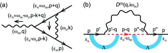
Figure 5: (a) First order correction of the electron-phonon vertex beyond Migdal’s approximation. The wavy lines represent phonons and the solid lines represent the fermions. (b) The electron-phonon interaction induced self-energies dressed by Diffuson.

V The vertex correction beyond Migdal’s approximation

In this section, we will show that the vertex correction has the order of $c_{s}/v_{F}$ which is relatively small and can be neglected in the present work. According to the rules for the Feynman diagrams depicted as Fig. S1(a), the first order perturbation vertex correction beyond the Migdal’s approximation can be expressed as

$$\Gamma(p,q)=\frac{1}{\beta V}\sum_{\omega_{s}}\sum_{\mathbf{k}}M_{\mathbf{k}}^{2}G^{(0)}(\epsilon_{n}-\omega_{s},\mathbf{p}-\mathbf{k})G(\epsilon_{n}-\omega_{s}+\omega_{m},\mathbf{p}-\mathbf{k}+\mathbf{q})D(\omega_{s},\mathbf{k}),$$

where $D^{(0)}$ and $G^{(0)}$ are the electron and phonon Green’s function in the absence of interaction. We consider the external variables $\epsilon_{n}=0$ and $\mathbf{p}=0$, which is the crucial case for our further calculations,

$$\Gamma(\omega_{m},q)=\sum_{\zeta,\zeta^{\prime}}\sum_{\omega_{s}}\sum_{\mathbf{k}}M_{\mathbf{k}}^{2}\frac{-2\omega_{\mathbf{k}}}{\omega_{s}^{2}+\omega_{\mathbf{k}}^{2}}\frac{\mathcal{P}_{\zeta}(\mathbf{k})}{i\omega_{s}-\xi_{\mathbf{k}}^{\zeta}}\frac{\mathcal{P}_{\zeta^{\prime}}(\mathbf{q}-\mathbf{k})}{i(\omega_{s}-\omega_{m})-\xi_{\mathbf{k}-\mathbf{q}}^{\zeta^{\prime}}}.$$ (20)

Notice that the dominant contribution in Eq. (20) arises from the region of $\mathbf{k}$ space where the integrand has a vanishing demonimator. Thus, we restrict our consideration to the states crossing the Fermi energy $\zeta=\zeta^{\prime}=+$, such that we can drop the band indices. By projecting onto the identity matrix, substituting the electron-phonon coupling strength $M_{\mathbf{k}}^{2}=\frac{\hbar c_{s}|\mathbf{k}|\Xi^{2}}{2V\varrho c_{s}^{2}}$ and taking zero-temperature limit $T\sum_{\omega}\to\int_{-\infty}^{\infty}\frac{d\omega}{2\pi}$ , we have

$$\Gamma(\omega_{m},q)=\frac{\gamma}{2\pi}\int_{-E_{c}}^{E_{c}}dE\int_{-\infty}^{\infty}d\omega\frac{1}{2}\int_{-1}^{1}dx\frac{\omega_{0}}{i\omega-E}\frac{-2\omega_{0}}{\omega^{2}+\omega_{0}^{2}}\frac{1}{i(\omega-\omega_{m})-(E-v_{F}qx)}.$$

Here we have truncated to the linear order of the momentum and consider a locally linear dispersion of the band in the vicinity of $k_{F}$, $\xi_{\mathbf{k}}=\epsilon_{\mathbf{k}}-\mu\approx v_{F}|\mathbf{k}|-\mu\equiv E$ and $\xi_{\mathbf{k}-\mathbf{q}}=\epsilon_{\mathbf{k}-\mathbf{q}}-\mu\approx v_{F}|\mathbf{k}-\mathbf{q}|-\mu\approx E-v_{F}|\mathbf{q}|\cos\theta$ with $\theta$ is the scattering angle and introduced new integration variables $E=v_{F}|\mathbf{k}|-\mu$ and $x=\cos\theta$. We choose an energy cutoff of the order of Fermi energy $E_{c}\sim\hbar v_{F}k_{F}$. Since we only work to the orders of magnitude, the density of state $\nu$ is assumed to be constant between $-E_{c}$ and $E_{c}$ and the phonon’s energy is approximated as $\omega_{\mathbf{k}}\approx\hbar c_{s}k_{F}\equiv\omega_{0}$. $\gamma=\frac{\Xi^{2}\nu}{2\varrho c_{s}^{2}}$ is the dimensionless coupling strength. Then, we first evaluate the integration over $\omega$, it is convenient to split the integrand into sum of relatively simple terms:

$$\Gamma(\omega_{m},q) =-\gamma\int_{-E_{c}}^{E_{c}}dx\frac{1}{2}\int_{-1}^{1}dx\frac{\omega_{0}}{\omega_{m}+iv_{F}qx}\int_{-\infty}^{\infty}d\omega\frac{1}{2\pi i}\Bigg{[}\frac{1}{(\omega-\omega_{m})+i(E-v_{F}qx)}\frac{1}{\omega+i\omega_{0}}-\frac{1}{\omega+ix}\frac{1}{\omega+i\omega_{0}}$$

$$-\frac{1}{(\omega-\omega_{m})+i(E-v_{F}qx)}\frac{1}{\omega-i\omega_{0}}+\frac{1}{\omega+iE}\frac{1}{\omega-i\omega_{0}}\Bigg{]}.$$

Only when the singularities of two energy denominators are on the opposite side of the real axis, the integration will not vanish, which leads to

$$\Gamma(\omega_{m},q) =-\gamma\int_{-E_{c}}^{E_{c}}dE\frac{1}{2}\int_{-1}^{1}dx\frac{\omega_{0}}{\omega_{m}+iv_{F}qx}\Bigg{[}\frac{\theta(-E+v_{F}qx)}{\omega_{m}-i(E-v_{F}qx)+i\omega_{0}}-\frac{\theta(-E)}{-iE+i\omega_{0}}$$

$$-\frac{\theta(E-v_{F}qx)}{i\omega_{0}-\omega_{m}+i(E-v_{F}qx)}+\frac{\theta(E)}{i\omega_{0}+iE}\Bigg{]}.$$

where $\theta(x)$ is the Heaviside step function. The second and the forth terms in the bracket cancel each other when integrating over $E$. Performing $E$ integration, the other two terms gives,

$$\Gamma(\omega_{m},q) =-\gamma\int_{-1}^{1}dx\frac{1}{(v_{F}qx)^{2}+\omega_{m}^{2}}\Bigg{\{}\frac{1}{2}v_{F}qx\log\left(\frac{\omega_{m}^{2}+(E_{c}+\omega_{0}-v_{F}qx)^{2}}{\omega_{m}^{2}+\omega_{0}^{2}}\right)$$

$$-\omega_{m}\left[\tan^{-1}\left(\frac{\omega_{m}}{E_{c}+\omega_{0}-v_{F}qx}\right)-\tan^{-1}\left(\frac{\omega_{m}}{\omega_{0}}\right)\right]\Bigg{\}}.$$

In order to proceed with the $x$ integration we further expand the integrand for small value of $q$ up to quadratic terms. After the integration, we arrive at the expression for vertex function,

$$\Gamma(\omega_{m},q) =-2\gamma\frac{\omega_{0}}{v_{F}q}\Bigg{\{}\left[\tan^{-1}\left(\frac{\omega_{m}}{\omega_{0}}\right)-\tan^{-1}\left(\frac{\omega_{m}}{E_{c}+\omega_{0}}\right)\right]\tan^{-1}\frac{v_{F}q}{\omega_{m}}$$

$$-\frac{\omega_{m}(E_{c}+\omega_{0})}{(E_{c}+\omega_{0})^{2}+\omega_{m}^{2}}\left[1+\frac{\omega_{m}^{2}}{(E_{c}+\omega_{0})^{2}+\omega_{m}^{2}}\right]\left(\frac{v_{F}q}{\omega_{m}}+\tan^{-1}\frac{v_{F}q}{\omega_{m}}\right)\Bigg{\}}.$$

Now we consider the static limit by taking $\omega_{m}\to 0$ first and then $q\to 0$,

$$\lim_{q\to 0}\lim_{\omega_{m}\to 0}\Gamma(\omega_{m},q)=-\gamma\frac{2\omega_{0}}{E_{c}+\omega_{0}}=-2\gamma\frac{c_{s}}{v_{F}+c_{s}}$$

When the velocity of sound $(c_{s})$ is much smaller than the Fermi velocity $(v_{F})$ which is typically the situation in solid state materials, the correction to the electron-phonon vertex is suppressed by a factor $c_{s}/v_{F}$ and can be safely neglected.

VI The vertex corrections to the electron-phonon self-energy from disorder effect

In the theory of disordered noninteraction system, the disordered averaged product of Green’s functions in the particle-hole polarization bubble gives the “diffusion” mode at low frequencies and momenta ($|\omega|,v_{F}q\ll\tau_{0}^{-1}$, the so-called diffusion approximation, with $v_{F}$ is the Fermi velocity). The diffusion mode will introduce a vertex correction to the electron-phonon vertices,

$$M_{\mathrm{diff}}(\mathbf{q},i\omega_{n})=M_{\mathbf{q}}\Lambda(\mathbf{q},i\omega_{n}).$$

The particle-hole diffusion vertex $\Lambda(\mathbf{q},i\omega_{n})$ can be calculated through the summation of the ladder diagrams,

$$\Lambda(\mathbf{q},i\omega_{n})=[1-P(\mathbf{q},i\omega_{n})]^{-1},$$

with

$$P(\mathbf{q},i\omega_{n}) =\frac{1}{2\pi\nu\tau_{0}}\int\frac{d^{3}\mathbf{k}}{(2\pi)^{3}}\mathrm{Tr}[G(\mathbf{k}-\mathbf{q},i\epsilon_{m}-i\omega_{n})G(\mathbf{k},i\epsilon_{m})].$$

This integration vanishes unless the poles of the two Green’s functions locate on the opposite sides of the real axis of the complex plane, the particle-hole diffusion vertex can be obtained as,

$$\Lambda(\mathbf{q},i\omega_{n})=\frac{\theta[\epsilon_{m}(\omega_{n}-\epsilon_{m})]}{\tau_{0}\left(|\omega_{n}|+\mathcal{D}\mathbf{q}^{2}\right)},$$

with the noninteracting diffusion constant $\mathcal{D}=v_{F}^{2}\tau_{0}/3$ and $\tau_{0}$ is the elastic relaxation time induced by disorder effect. Then the electron-phonon self-energy with vertex correction from disorder effect [shown as Fig. S1(b)] is given by

$$\Sigma_{ep}^{\prime}(\mathbf{p},i\epsilon_{m}) =-\frac{1}{\beta}\sum_{i\omega_{n},\mathbf{q}}\frac{|M_{\mathbf{q}}|^{2}D^{(0)}(\mathbf{q},i\omega_{n})\theta(\epsilon_{m}(\omega_{n}-\epsilon_{m}))}{(|\omega_{n}|+\mathcal{D}\mathbf{q}^{2})^{2}\tau_{0}^{2}}\hat{G}^{(0)}(\mathbf{p}-\mathbf{q},i\epsilon_{m}-i\omega_{n})$$

$$=\frac{\Xi^{2}}{\varrho c_{s}^{2}}\frac{1}{\beta V}\sum_{\mathbf{q}}\sum_{\omega_{n}-\epsilon_{m}>0}\frac{1}{(|\omega_{n}|+\mathcal{D}\mathbf{q}^{2})^{2}\tau_{0}^{2}}\hat{G}^{(0)}(\mathbf{p}-\mathbf{q},i\epsilon_{m}-i\omega_{n}),$$

where the summation over $\omega_{n}$ is restricted to the region of $\epsilon_{m}(\omega_{n}-\epsilon_{m})>0$. For $|\mathbf{p}|\sim k_{F}$ and $\epsilon_{m}>0$ ($\epsilon_{m}\to 0$), since the dominant contributions in the integrations are due to both small $q$ and small $|\omega_{n}|$, $\hat{G}^{(0)}(\mathbf{p}+\mathbf{q},i\epsilon_{m}-i\omega_{n})$ can be approximated by $2\tau_{0}i$ and the $\mathbf{q}$ and $\omega_{n}$ dependences of $|M_{\mathbf{q}}|^{2}D^{(0)}(\mathbf{q},i\omega_{n})\approx\frac{\Xi^{2}}{V\varrho c_{s}^{2}}$ can be ignored,

$$\Sigma_{ep}^{\prime}(\mathbf{p},i\epsilon_{m})=2\tau_{0}^{-1}i\frac{\Xi^{2}}{\varrho c_{s}^{2}}\frac{1}{\beta V}\sum_{\mathbf{q}}\sum_{\omega_{n}-\epsilon_{m}>0}\frac{1}{(|\omega_{n}|+\mathcal{D}\mathbf{q}^{2})^{2}}$$

after performing the $\mathbf{q}$ integration,

$$\Sigma_{ep}^{\prime}(\mathbf{p},i\epsilon_{m})=2\tau_{0}^{-1}i\frac{\Xi^{2}}{\varrho c_{s}^{2}}\frac{1}{8\pi\mathcal{D}^{3/2}}\frac{1}{\beta}\sum_{\omega_{n}-\epsilon_{m}>0}\frac{1}{\sqrt{|\omega_{n}|}},$$ (21)

where the summations over $\omega_{n}$ is up to $|\omega_{n}|=\tau_{0}^{-1}$ which corresponds a upper bound of the summation $n_{c}=(2\pi\tau_{0}k_{B}T)^{-1}$ ,

$$\Sigma_{ep}^{\prime}(\mathbf{p},\epsilon)=2\tau_{0}^{-1}i\frac{\Xi^{2}}{\varrho c_{s}^{2}}\frac{\sqrt{k_{B}T}}{4(2\pi\mathcal{D})^{3/2}}\left[\zeta(\frac{1}{2},\frac{\epsilon}{2\pi k_{B}T}+\frac{1}{2})-\zeta(\frac{1}{2},\frac{1}{2\pi\tau_{0}k_{B}T}+1)\right].$$

At $T=0$ and $|\epsilon|\ll 1/\tau_{0}$, from Eq. (21), we have

$$\Sigma_{ep}^{\prime}(\mathbf{p},\epsilon)=\tau_{0}^{-1}i\frac{\Xi^{2}}{\varrho c_{s}^{2}}\frac{1}{8\pi^{2}\mathcal{D}^{3/2}}\int_{\epsilon}^{\tau_{0}^{-1}}dx\frac{1}{\sqrt{x}}\approx i\frac{\Xi^{2}}{\varrho c_{s}^{2}}\frac{3\sqrt{3}}{4\pi^{2}(\hbar v_{F})^{3}}.$$

For $T\neq 0$, and $\epsilon\ll k_{B}T$,

$$\Sigma_{ep}^{\prime}(\mathbf{p},\epsilon)\approx 2\tau_{0}^{-1}i\frac{\Xi^{2}}{\varrho c_{s}^{2}}\frac{\sqrt{k_{B}T}}{4(2\pi\mathcal{D})^{3/2}}\left[\zeta(\frac{1}{2},\frac{\epsilon}{2\pi k_{B}T}+\frac{1}{2})-\zeta(\frac{1}{2},\frac{1}{2\pi\tau_{0}k_{B}T}+1)\right]$$

where $\zeta(s,a)$ is the Hurwitz zeta function with the asymptotic expansion for large argument as

$$\zeta(s,a)\sim\frac{a^{1-s}}{s-1}+\frac{1}{2}a^{-s}+\cdots.$$

The second term in the blanket gives a constant contribution independent of $\epsilon$ and $k_{B}T$ which can be absorbed into the disorder induced self-energy. Let us consider only the first term. For $|\epsilon|\gg k_{B}T$, we have

$$\Sigma_{ep}^{\prime}(\mathbf{p},\epsilon)\sim-\tau_{0}^{-1}i\frac{\Xi^{2}}{\varrho c_{s}^{2}}\frac{\sqrt{\epsilon}}{4\pi^{2}(\mathcal{D})^{3/2}},$$

and for $|\epsilon|\ll k_{B}T$,

$$\Sigma_{ep}^{\prime}(\mathbf{p},\epsilon)\sim 2\tau_{0}^{-1}i\frac{\Xi^{2}}{\varrho c_{s}^{2}}\frac{\sqrt{k_{B}T}}{4(2\pi\mathcal{D})^{3/2}}\zeta(\frac{1}{2},\frac{1}{2}).$$

This mixing effect from EPI and the disorder only modifies the imaginary part of the self-energy when the temperature is very low. In the classical regime $(T>\Theta_{D})$, this higher order correction becomes negligible. We believe the lowest order perturbation theory may adequately account for these observed anomalous transport properties.

VII Finite temperature conductivity

After having the self-energy from the EPI, we can calculate the transport quantities. To distinguish from the quantities of the non-interacting case, all renormalized quantities such as the effective mass, the effective chemical potential, and the effective velocity will be denoted with a bar overhead. In the Kubo-Streda formalism of the linear response theory (streda1982quantised, ; Wang18prb, ), the conductivity tensor can be expressed by means of the Green’s functions,

$$\sigma_{ij}=\sigma_{ij}^{(1)}+\sigma_{ij}^{(2)}+\sigma_{ij}^{(3)}$$ (22)

with

$$\sigma_{ij}^{(1)}= \frac{\hbar e^{2}}{4\pi V}\int_{-\infty}^{+\infty}d\epsilon n_{F}^{\prime}(\epsilon-\bar{\mu})\text{Tr}\left[\hat{v}_{i}(G^{R}(\epsilon)-G^{A}(\epsilon))\hat{v}_{j}(G^{R}(\epsilon)-G^{A}(\epsilon))\right]$$ (23)

$$\sigma_{ij}^{(2)}= -\frac{\hbar e^{2}}{4\pi V}\int_{-\infty}^{+\infty}d\epsilon n_{F}^{\prime}(\epsilon-\bar{\mu})\text{Tr}\left[\left(\hat{v}_{i}G^{R}(\epsilon)v_{j}-\hat{v}_{j}G^{R}(\epsilon)\hat{v}_{i}\right)G^{A}(\epsilon)\right]$$ (24)

$$\sigma_{ij}^{(3)}= \frac{\hbar e^{2}}{4\pi V}\int_{-\infty}^{+\infty}d\epsilon n_{F}(\epsilon-\bar{\mu})\text{Tr}\Bigg{[}\left(\hat{v}_{i}G^{R}(\epsilon)\hat{v}_{j}-\hat{v}_{j}G^{R}(\epsilon)\hat{v}_{i}\right)\frac{dG^{R}(\epsilon)}{d\epsilon}$$

$$-\left(\hat{v}_{i}G^{A}(\epsilon)\hat{v}_{j}-\hat{v}_{j}G^{A}(\epsilon)\hat{v}_{i}\right)\frac{dG^{A}(\epsilon)}{d\epsilon}\Bigg{]}$$ (25)

where $\sigma_{ij}^{(1)}$ is symmetric with respect to $i$ and $j$ and contributes to the diagonal elements of the conductivity tensor, whereas $\sigma_{ij}^{(2)}$ and $\sigma_{ij}^{(3)}$ are antisymmetric and contribute to the off diagonal elements. $\hat{v}_{i}=\frac{1}{\hbar}\frac{\partial\mathcal{H}_{Dirac}}{\partial k_{i}}$ is the velocity operator for Dirac materials. It is convenient to work in the basis of the effective Hamiltonian $\mathcal{H}_{eff}(\mathbf{k})=\mathcal{H}_{Dirac}(\mathbf{k})+\mathrm{Re}\Sigma_{ep}^{R}(\boldsymbol{0},0)$. In this basis, the velocity in $x,y$ direction can be obtained as $\widetilde{v}_{\perp}^{\zeta}(k)=\frac{1}{\hbar}\frac{\partial\bar{\xi}_{\mathbf{k}}}{\partial k_{x}}$ and the Green’s function can be expressed as $\bar{G}_{\zeta}^{R}(\mathbf{k},\epsilon)=[\epsilon-\bar{\xi}_{\mathbf{k}}^{\zeta}-i\mathrm{Im}\Sigma^{R}(\mathbf{k},\bar{\xi}_{\mathbf{k}}^{\zeta})]^{-1}$, where $\mathrm{Im}\Sigma^{R}(\mathbf{k},\bar{\xi}_{\mathbf{k}}^{\zeta})=\mathrm{Im}\Sigma_{ep}^{R}(\mathbf{k},\bar{\xi}_{\mathbf{k}}^{\zeta})+\mathrm{Im}\Sigma_{imp}^{R}(\mathbf{k},\bar{\xi}_{\mathbf{k}}^{\zeta})$. Then the relaxation time can be obtained $\tau_{\zeta}(\mathbf{k})=\hbar/[-2\mathrm{Im}\Sigma^{R}(\mathbf{k},\bar{\xi}_{\mathbf{k}}^{\zeta})]$. $n_{F}^{\prime}(\epsilon-\bar{\mu})\equiv dn_{F}(\epsilon-\bar{\mu})/d\epsilon$ is the energy derivative of the Fermi-Dirac distribution function $n_{F}(\epsilon-\bar{\mu})$.

In the absence of magnetic field, due to the combined time-reversal and inversion symmetry of the Dirac Hamiltonian, the off diagonal components of the conductivity tensor vanish, the longitudinal conductivity can be evaluated from $\sigma_{ij}^{(1)}=\delta_{ij}\sigma_{D}$(Akkermans2007, ),

$$\sigma_{D}(T)=\int_{|\bar{m}|}^{\infty}d\omega(-n_{F}^{\prime}(\omega-\bar{\mu}))\sigma_{+}(\omega)+\int_{-\infty}^{-|\bar{m}|}d\omega(-n_{F}^{\prime}(\omega-\bar{\mu}))\sigma_{-}(\omega),$$ (26)

with the conductivities for the electron ($\zeta=+$) and hole ($\zeta=-$) carriers,

$$\sigma_{\zeta}(\omega)=2e^{2}\bar{\nu}_{\zeta}(\omega)\bar{D}_{\zeta}(\omega),$$ (27)

where the diffusion constants for two types of carriers are defined as $\bar{D}_{\zeta}(\mu)=\frac{1}{3}\langle(\widetilde{v}_{\perp}^{\zeta})^{2}\rangle_{FS}\bar{\tau}_{\zeta}(\bar{q}_{\omega})$. In the presence of magnetic field $B$, say, along the z-direction, the conductivity tensor can be evaluated in the Landau level representation. Here we are only interested in the semiclassical regime that the self-energy corrections can be approximated as the zero field results. In this regime, the transverse conductivity can be calculated as

$$\sigma_{xx}(B,T)=\int_{|\bar{m}|}^{\infty}d\omega\frac{-n_{F}^{\prime}(\omega-\bar{\mu})\sigma_{+}(\omega)}{[\chi_{+}(\omega)B]^{2}+1}+\int_{-\infty}^{-|\bar{m}|}d\omega\frac{-n_{F}^{\prime}(\omega-\bar{\mu})\sigma_{-}(\omega)}{[\chi_{-}(\omega)B]^{2}+1},$$ (28)

and the anomalous part of Hall conductivity $\sigma_{ij}^{(3)}$ can be neglected, the expression of the Hall conductivity in this case reads

$$\sigma_{xy}(B,T)=\int_{|\bar{m}|}^{\infty}d\omega\frac{-n_{F}^{\prime}(\omega-\bar{\mu})\sigma_{+}(\omega)\chi_{+}(\omega)B}{[\chi_{+}(\omega)B]^{2}+1}+\int_{-\infty}^{-|\bar{m}|}d\omega\frac{-n_{F}^{\prime}(\omega-\bar{\mu})\sigma_{-}(\omega)\chi_{-}(\omega)B}{[\chi_{-}(\omega)B]^{2}+1}$$ (29)

where $\chi_{\pm}(\omega)=e\bar{\tau}_{\pm}(\omega)/\bar{m}^{*}$ are the mobilities for the conduction and valance bands with the cyclotron mass $m^{*}=\frac{1}{2}\frac{dq_{\perp}^{2}}{d\mu}$, respectively. The mobilities for two bands are strongly energy-dependent and can vary by orders of magnitude. The resistivity can be obtained by inverting the conductivity tensor. Then, the Hall resistivity $\rho_{xy}=\sigma_{xy}/[\sigma_{xx}^{2}+\sigma_{xy}^{2}]$ and the transverse resistivity $\rho_{xx}=\sigma_{xx}/[\sigma_{xx}^{2}+\sigma_{xy}^{2}]$ . In a weak magnetic field, the Hall resistivity exhibits a linear dependence with applied magnetic fields. Thus, the Hall coefficient $R_{H}$ is defined as the ratio of the Hall resistivity and the applied magnetic field,

$$R_{H}(T)=\frac{d\rho_{xy}(B,T)}{dB}\Big{|}_{B=0}.$$ (30)

The general expressions for the longitudinal and Hall parts of the thermoelectric coefficients are

$$\alpha_{xx}(B,T) =\frac{1}{eT}\int_{|\bar{m}|}^{\infty}d\omega\left(\omega-\bar{\mu}\right)\frac{-n_{F}^{\prime}(\omega-\bar{\mu})\sigma_{+}(\omega)}{[\chi_{+}(\omega)B]^{2}+1}+\frac{1}{eT}\int_{-\infty}^{-|\bar{m}|}d\omega\left(\omega-\bar{\mu}\right)\frac{-n_{F}^{\prime}(\omega-\bar{\mu})\sigma_{-}(\omega)}{[\chi_{-}(\omega)B]^{2}+1},$$ (31)

$$\alpha_{xy}(B,T) =\frac{1}{eT}\int_{|\bar{m}|}^{\infty}d\omega\left(\omega-\bar{\mu}\right)\frac{-n_{F}^{\prime}(\omega-\bar{\mu})\sigma_{+}(\omega)\chi_{+}(\omega)B}{[\chi_{+}(\omega)B]^{2}+1}+\frac{1}{eT}\int_{-\infty}^{-|\bar{m}|}d\omega\left(\omega-\bar{\mu}\right)\frac{-n_{F}^{\prime}(\omega-\bar{\mu})\sigma_{-}(\omega)\chi_{-}(\omega)B}{[\chi_{-}(\omega)B]^{2}+1}.$$ (32)

The Seebeck coefficient $S_{xx}$ and the Nernst signal $S_{xy}$ thus are given by

$$S_{xx} =\frac{\alpha_{xx}\sigma_{xx}+\alpha_{xy}\sigma_{xy}}{\sigma_{xx}^{2}+\sigma_{xy}^{2}},$$ (33)

$$S_{xy} =\frac{\alpha_{xy}\sigma_{xx}-\alpha_{xx}\sigma_{xy}}{\sigma_{xx}^{2}+\sigma_{xy}^{2}}.$$ (34)

References

- (1) S. Okada, T. Sambongi, M. Ido, Giant resistivity anomaly in . J. Phys. Soc. Jpn. 49, 839-840 (1980).
- (2) M. Izumi, K. Uchinokura, E. Matsuura, Anomalous electrical resistivity in HfTe5. Solid State Commun. 37, 641-642 (1981).
- (3) F. DiSalvo, R. Fleming, J. Waszczak, Possible phase transition in the quasi-one-dimensional materials or . Phys. Rev. B 24, 2935 (1981).
- (4) S. Okada, T. Sambongi, M. Ido, Y. Tazuke, R. Aoki, O. Fujita, Negative evidences for charge/spin density wave in . J. Phys. Soc. Jpn. 51, 460-467 (1982).
- (5) D. Bullett, Absence of a phase transition in. Solid State Commun. 42, 691-693 (1982).
- (6) H. Fjellvag, A. Kjekshus, Structural properties of and as seen by powder diffraction. Solid State Commun. 60, 91-93 (1986).
- (7) M. Izumi, K. Uchinokura, E. Matsuura, S. Harada, Hall effect and transverse magnetoresistance in a low-dimensional. Solid State Commun. 42, 773-778 (1982).
- (8) T. Jones, W. Fuller, T. Wieting, F. Levy, Thermoelectric power of and . Solid State Commun. 42, 793-798 (1982).
- (9) R. T. Littleton Iv, T. M. Tritt, J. W. Kolis, and D. Ketchum, Transition-metal pentatellurides as potential low-temperature thermoelectric refrigeration materials. Phys. Rev. B 60, 19453 (1999).
- (10) T. M. Tritt, N. D. Lowhorn, R. T. Littleton Iv, A. Pope, C. R. Feger, and J. W. Kolis, Large enhancement of the resistive anomaly in the pentatelluride materials and with applied magnetic field. Phys. Rev. B 60, 7816 (1999).
- (11) H. Weng, X. Dai, Z. Fang, Transition-metal pentatelluride and : a paradigm for large-gap quantum spin Hall insulators. Phys. Rev. X 4, 011002 (2014).
- (12) Z.-G. Chen, R. Chen, R. Zhong, J. Schneeloch, C. Zhang, Y. Huang, F. Qu, R. Yu, Q. Li, G. Gu, N. Wang, Spectroscopic evidence for bulk-band inversion and three-dimensional massive Dirac fermions in . Proc. Natl. Acad. Sci. U.S.A. 114, 816-821 (2017).
- (13) G. Manzoni, L. Gragnaniello, G. AutÚs, T. Kuhn, A. Sterzi, F. Cilento, M. Zacchigna, V. Enenkel, I. Vobornik, L. Barba, F. Bisti, Ph. Bugnon, A. Magrez, V. N. Strocov, H. Berger, O. V. Yazyev, M. Fonin, F. Parmigiani, A. Crepaldi, Evidence for a strong topological insulator phase in . Phys. Rev. Lett. 117, 237601 (2016).
- (14) Y. Jiang, J. Wang, T. Zhao, Z. L. Dun, Q. Huang, X. S. Wu, M. Mourigal, H. D. Zhou, W. Pan, M. Ozerov, D. Smirnov, and Z. Jiang, Unraveling the topological phase of via magnetoinfrared spectroscopy. Phys. Rev. Lett. 125, 046403 (2020).
- (15) Q. Li, D. E. Kharzeev, C. Zhang, Y. Huang, I. Pletikosic, A. Fedorov, R. Zhong, J. Schneeloch, G. Gu, T. Valla, Chiral magnetic effect in . Nat. Phys. 12, 550-554 (2016).
- (16) Y. Zhou, J. Wu, W. Ning, N. Li, Y. Du, X. Chen, R. Zhang, Z. Chi, X. Wang, X. Zhu, P.o Lu, C. Ji, X. Wan, Z. Yang, J. Sun, W. Yang, M. Tian, Y. Zhang, and H.-k. Mao, Pressure-induced superconductivity in a three-dimensional topological material . Proc. Nat. Acad. Sci. USA, 113, 2904 (2016).
- (17) P. Li, C. H. Zhang, J. W. Zhang, Y. Wen, and X. X. Zhang, Giant planar Hall effect in the Dirac semimetal , Phys. Rev. B 98, 121108(R) (2018).
- (18) H. Wang, H. Liu, Y. Li, Y. Liu, J. Wang, J. Liu, J.-Y. Dai, Y. Wang, L. Li, J. Yan, D. Mandrus, X. C. Xie and J. Wang, Discovery of log-periodic oscillations in ultraquantum topological materials. Sci. Adv. 4, eaau5096 (2018).
- (19) H. Wang, Y. Liu, Y. Liu, C. Xi, J. Wang, J. Liu, Y. Wang, L. Li, S. P. Lau, M. Tian, J. Yan, D. Mandrus, J. Y. Dai, H. Liu, X. C. Xie, J. Wang, Log-periodic quantum magneto-oscillations and discrete-scale invariance in topological material HfTe5. Natl. Sci. Rev. 6, 914-920 (2019).
- (20) T. Liang, J. Lin, Q. Gibson, S. Kushwaha, M. Liu, W. Wang, H. Xiong, J. A. Sobota, M. Hashimoto, P. S. Kirchmann, Z. Shen, R. J. Cava, N. P. Ong, Anomalous Hall effect in . Nat. Phys. 14, 451-455 (2018).
- (21) J. L. Zhang, C. M. Wang, C. Y. Guo, X. D. Zhu, Y. Zhang, J. Y. Yang, Y. Q. Wang, Z. Qu, L. Pi, H.-Z. Lu, and M. L. Tian, Anomalous thermoelectric effects of in and beyond the quantum limit. Phys. Rev. Lett. 123, 196602 (2019).
- (22) J. Hu, M. Caputo, E. B. Guedes, S. Tu, E. Martino, A. Magrez, H. Berger, J. H. Dil, H. Yu, J.-P. Ansermet, Large magnetothermopower and anomalous Nernst effect in . Phys. Rev. B 100, 115201 (2019).
- (23) F. Tang, Y. Ren, P. Wang, R. Zhong, J. Schneeloch, S. A. Yang, K. Yang, P. A. Lee, G. Gu, Z. Qiao, L. Zhang, Three-dimensional quantum Hall effect and metal-insulator transition in . Nature 569, 537-541 (2019).
- (24) P. Wang, Y. Ren, F. Tang, P. Wang, T. Hou, H. Zeng, L. Zhang, Z. Qiao, Approaching three-dimensional quantum Hall effect in bulk . Phys. Rev. B 101, 161201 (2020).
- (25) R. Y. Chen, S. J. Zhang, J. A. Schneeloch, C. Zhang, Q. Li, G. D. Gu, and N. L. Wang, Optical spectroscopy study of the three-dimensional Dirac semimetal , Phys. Rev. B 92, 075107 (2015).
- (26) L.-X. Zhao, X.-C. Huang, Y.-J. Long, D. Chen, H. Liang, Z.-H. Yang, M.-Q. Xue, Z.-A. Ren, H.-M. Weng, Z. Fang, X. Dai, G.-F. Chen, Anomalous Magneto-Transport Behavior in Transition Metal Pentatelluride , Chin. Phys. Lett. 34, 037102 (2017).
- (27) P. Shahi, D. J. Singh, J. P. Sun, L. X. Zhao, G. F. Chen, Y. Y. Lv, J. Li, J.-Q. Yan, D. G. Mandrus, J.-G. Cheng, Bipolar conduction as the possible origin of the electronic transition in pentatellurides: metallic vs semiconducting behavior. Phys. Rev. X 8, 021055 (2018).
- (28) B. Xu, L. Zhao, P. Marsik, E. Sheveleva, F. Lyzwa, Y. Dai, G. Chen, X. Qiu, C. Bernhard, Temperature-driven topological phase transition and intermediate Dirac semimetal phase in . Phys. Rev. Lett. 121, 187401 (2018).
- (29) Y. Zhang, C. Wang, L. Yu, G. Liu, A. Liang, J. Huang, S. Nie, X. Sun, Y. Zhang, B. Shen, J. Liu, H. Weng, L. Zhao, G. Chen, X. Jia, C. Hu, Y. Ding, W. Zhao, Q. Gao, C. Li, S. He, L. Zhao, F. Zhang, S. Zhang, F. Yang, Z. Wang, Q. Peng, X. Dai, Z. Fang, Z. Xu, C. Chen, X. Zhou, Electronic evidence of temperature-induced Lifshitz transition and topological nature in . Nat. Commun. 8, 15512 (2017).
- (30) Y. Zhang, C. Wang, G. Liu, A. Liang, L. Zhao, J. Huang, Q. Gao, B. Shen, J. Liu, C. Hu, W. Zhao, G. Chen , X. Jia, L. Yu, L. Zhao , S. He, F. Zhang, S. Zhang, F. Yang, Z. Wang, Q. Peng, Z. Xu, C. Chen, X. Zhou, Temperature-induced Lifshitz transition in topological insulator candidate . Sci. Bull. 62, 950-956 (2017).
- (31) M. Rubinstein, and : Possible polaronic conductors. Phys. Rev. B 60, 1627 (1999).
- (32) R. Wu, J.-Z. Ma, S.-M. Nie, L.-X. Zhao, X. Huang, J.-X. Yin, B.-B. Fu, P. Richard, G.-F. Chen, Z. Fang, X. Dai, H.-M. Weng, T. Qian, H. Ding, S. H. Pan, Evidence for topological edge states in a large energy gap near the step edges on the surface of . Phys. Rev. X 6, 021017 (2016).
- (33) X.-B. Li, W.-K. Huang, Y.-Y. Lv, K.-W. Zhang, C.-L. Yang, B.-B. Zhang, Y. B. Chen, S.-H. Yao, J. Zhou, M.-H. Lu, L. Sheng, S.-C. Li, J.-F. Jia, Q.-K. Xue, Y.-F. Chen, D.-Y. Xing, Experimental observation of topological edge states at the surface step edge of the topological insulator . Phys. Rev. Lett. 116, 176803 (2016).
- (34) G. D. Mahan, Many-Body Physics (Plenum Press, New York, ed.2,1990).
- (35) S. Q. Shen, Topological Insulators (Springer, Singapore, ed. 2, 2017), vol. 187 of Springer Series in Solid-State Sciences.
- (36) See Supplemental Material at [URL to be added by publisher] for details of (Sec. SI) the model Hamiltonian for Anisotropic Dirac materials (Sec. SII) the model for electron-phonon interaction, (Sec. SIII) the phonon-induced self-energy, (Sec. SIV) the renormalization of the energy level of Dirac polaron, (Sec. SV) the vertex correction beyond Migdal’s approximation, (Sec. SVI) the vertex corrections to the electron-phonon self-energy from disorder effect, and (Sec. SVII) finite temperature conductivity, which includes Refs.(zhang2017temperature, ; Mahan-book, ; Migdal-58jetp, ; fu2007topological, ; zhu2018record, ; Aryal2020topological, ; zhang2020observation, ; streda1982quantised, ; Wang18prb, ; Akkermans2007, ).
- (37) L. Fu, and C. L. Kane, Topological insulators with inversion symmetry, Phys. Rev. B 76, 045302 (2007).
- (38) J. Zhu, T. Feng, S. Mills, P. Wang, X. Wu, L. Zhang, S. T. Pantelides, X. Du, X. Wang, Record-low and anisotropic thermal conductivity of a quasi-one-dimensional bulk ZrTe5 single crystal. ACS Appl. Mater. Interfaces 10, 40740 (2018).
- (39) N. Aryal, X. Jin, Q. Li, A. M. Tsvelik, and W. Yin, Topological phase transition and phonon-space Dirac topology surfaces. in ZrTe5, https://arxiv.org/pdf/2004.13326.pdf
- (40) W. Zhang, P. Wang, B. Skinner, R. Bi, V. Kozii, C.-W. Cho, R. Zhong, J. Schneeloch, D. Yu, G. Gu, L. Fu, X. Wu, L. Zhang, Observation of a thermoelectric Hall plateau in the extreme quantum limit, Nat. Commun. 11, 1046 (2020).
- (41) P. Streda, Quantised Hall effect in a two-dimensional periodic potential. J. Phys. C: Solid State Phys. 15, L1299 (1982).
- (42) H. W. Wang, B. Fu, and S. Q. Shen, Intrinsic magnetoresistance in three-dimensional Dirac materials with low carrier density. Phys. Rev. B 98, 081202(R) (2018).
- (43) E. Akkermans, and G. Montambaux. Mesoscopic physics of electrons and photons (Cambridge university press, England, 2007).
- (44) I. Garate, Phonon-Induced Topological Transitions and Crossovers in Dirac Materials, Phys. Rev. Lett. 110, 046402 (2013).
- (45) K. Saha and I. Garate, Phonon-induced topological insulation, Phys. Rev. B 89, 205103 (2014).
- (46) L. Moreschini, J. C. Johannsen, H. Berger, J. Denlinger, C. Jozwiack, E. Rotenberg, K. S. Kim, A. Bostwick, and M. Grioni, Nature and topological of the low-energy states in , Phys. Rev. B 94, 081101(R) (2016).
- (47) G. Manzoni, A. Sterzi, A. Crepaldi, M. Diego, F. Cilento, M. Zacchigna, Ph. Bugnon, H. Berger, A. Magrez, M. Grioni, and F. Parmigiani, Ultrafast Optical Control of the Electronic Properties of , Phys. Rev. Lett. 115, 207402 (2015).
- (48) A. B. Migdal, Interaction between electrons and lattice vibrations in a normal metal. Sov. Phys. JETP 34, 996-1001 (1958).
- (49) J. Mutch, W.-C. Chen, P. Went, T. Qian, I. Z. Wilson, A. Andreev, C.-C. Chen, J.-H. Chu, Evidence for a strain-tuned topological phase transition in . Sci. Adv. 5, eaav9771 (2019).
- (50) S. A. Miller, I. Witting, U. Aydemir, L. Peng, A. J. E. Rettie, P. Gorai, D. Y. Chung, M. G. Kanatzidis, M. Grayson, V. Stevanović, E. S. Toberer, and G. J. Snyder, Polycrystalline Parametrized as a Narrow-Band-Gap Semiconductor for Thermoelectric Performance, Phys. Rev. Appl. 9, 014025 (2018).
- (51) A. C. Niemann, J. Gooth, Y. Sun, F. Thiel, A. Thomas, C. Shekhar, V. Suß, C. Felser, and K. Nielsch, Magneto-thermoelectric characterization of a micro-ribbon, Appl. Phys. Lett. 115, 072109 (2019).
- (52) M. Cutler, N. F. Mott, Observation of Anderson Localization in an Electron Gas, Phys. Rev. 181, 1336 (1969).
- (53) G. S. Nolas, J. Sharp, H. J. Godsmid, Thermoelectrics: Basic Principles and New materials Developments. (Springer, Heidelberg, 2001) vol. 45 of Springer Series in material science.
- (54) H. Chi, C. Zhang, G. Gu, D. E. Kharzeev, X. Dai, Q. Li, Lifshitz transition mediated electronic transport anomaly in bulk . New J. Phys 19, 015005 (2017).
- (55) Y. -Y. Lv, X. Li, L. Cao, D. Lin, S. -H. Yao, S. -S. Chen, S. -T. Dong, J. Zhou, Y. B. Chen, and Y. -F. Chen, Tunable Resistance or Magnetoresistance Cusp and Extremely Large Magnetoresistance in Defect-Engineered Single Crystals, Phys. Rev. Appl. 9, 054049 (2018).
- (56) A. B. Pippard, Magnetoresistance in Metals (Cambridge University Press, New York, 1989).