Add force and/or change underlying projection method to improve accuracy of Explicit Robin-Neumann and fully decoupled schemes for the coupling of incompressible fluid with thin-walled structure

Abstract

This work aims at providing some novel and practical ideas to improve accuracy of some partitioned algorithms, precisely Fernandez’s Explicit Robin-Neumann and fully decoupled schemes, for the coupling of incompressible fluid with thin-walled structure. Inspired by viscosity of fluid and justified by boundary layer theory, the force between fluid and structure corresponding to viscosity is increased. Numerical experiments demonstrate improvement of accuracy under such modification. To improve accuracy of fully decoupled schemes further, the underlying projection method is replaced.

Keywords: viscosity, boundary layer, fluid-structure interaction, accuracy, Explicit Robin-Neumann scheme, fully decoupled scheme

1 Background

The coupling of incompressible fluid with thin-walled structure typically arises in bio-mechanics of blood flow in human arteries, for which the blood flow is viscous and incompressible, while the structure assumed to be deformable. The blood flow is supposed to be free of full-scale turbulence, since its Reynolds numbers in arteries are usually below $2000$ [15].

Among various algorithms on this topic, Fernandez’s Explicit Robin-Neumann [14] and fully decoupled schemes [11] [13] are exceptional, due to these features:

1. High efficiency. The fluid and structure are solved only once per time-step, in a genuinely partitioned style. The fully decoupled scheme is even more efficient than Explicit Robin-Neumann scheme, because the velocity and pressure of fluid are decoupled.

2. Unconditional stability free of added-mass effect proved by theoretical analysis or numerical experiments (availability of theoretical analysis depends on extrapolation orders).

3. First-order accuracy (under extrapolations of first- or second- order).

4. Applicability to the topic with a vast variety of structure models.

The other algorithms do not possess all these properties, to the best knowledge of the author of this work. Some are less efficient ([19] [25] [6]) or accurate ([7] [10] [12]), some are unstable independently of space or time parameters (e.g. the standard Dirichlet–Neumann explicit coupling scheme) or stable only under restrictive constraints on these parameters ([7] [10]), and others are only applicable to the interaction of fluid with specific structure due to the way of convergence analysis ([2] ).

Remark 1

Instability of some algorithms on this topic is believed to be induced by added-mass effect (see e.g. [15]). At the beginning, this work was initiated by the study of added-mass effect, but does not focus on it later, so here only presents some notes. In fluid mechanics, when a body moves in a fluid, the inertia of the fluid opposes the motion, because the body and the fluid can not occupy the physical space at the same time. It is equivalent to having a virtual mass added to the mass of the body [1] [17]. Such effect is named added mass effect. The concept was first investigated by Dubua (1776), who conducted experiments on spherical pendulum of low swings [4]. Exact mathematical expressions of added mass for a sphere were obtained by Green (1833) and Stokes (1843) respectively [23]. Later the concept was generalized to a desired body moving in different flow regimes [21]. Nobile et al. [8] analysed mathematically the added-mass effect for a linear, incompressible and inviscid fluid coupled with a linear, elastic and cylindrical tube and applied the analysis to some explicit and implicit schemes to prove their unconditional instabilities or find out the conditions of stabilities.

2 Motivation

Compared with fully implicit algorithms, partitioned algorithms are less accurate. This work aims at providing some novel and practical ideas to improve accuracy of some partitioned algorithms, precisely Fernandez’s Explicit Robin-Neumann and fully decoupled schemes, for the coupling of incompressible fluid with thin-walled structure.

From point of view of physical intuition, due to viscosity of fluid, when the structure moves, some amount of fluid is attached to it near the interface, resulting in some actual mass added to the structure. By Newton’s Second Law, the mass together with acceleration produces a force on the structure; on the other hand, viscosity causes skin friction between fluid and structure. By Newton’s Third Law, there is an equal and opposite force on the fluid. The application of Newton’s Third Law ensures balance of force.

The intuition can be justified by the theory of boundary layer, which was first introduced by Ludwig Prandtl in 1904 concerning the motion of a fluid with small viscosity near the wall of a solid boundary [26]. The theory states, adjacent to the wall, there exists a thin transition layer, within which the viscosity of fluid takes significant effect on the motion of fluid (in fact, inside the layer, the viscous force is so large that it is of the same order with inertia force). The layer is called boundary layer. Over decades, the theory grew and was validated by an amount of experimental observations in various scientific and engineering fields [27]. It is also worth noting that the pressure remains almost constant (in the senses that the pressure gradient is negligible) through the boundary layer in a direction normal to the interface.

Thus, it is reasonable to expect, for a partitioned algorithm, increasing the force between the fluid and structure due to viscosity of fluid can make it more realistic, namely more close to the actual behaviour of the coupling system, which might lead to better accuracy. The amount of extra force resulting from viscosity is difficult (if not impossible) to compute; however, it can be approached. Up to certain values, increasing the force gradually should improve accuracy gradually.

The idea is applied to Fernandez’s two schemes mentioned above. In what follows, the two schemes are presented. Afterwards, coefficients of the terms corresponding to force from viscosity are increased, generating Algorithm 1 and Algorithm 2. Fernandez’s fully decoupled scheme is based on Chorin-Temam projection method. To improve accuracy further, the underlying projection method is replaced with Van Kan’s, leading to Algorithm 3.

Numerical results are reported later. The results indicate improvement of accuracy as the force from viscosity increases. Appropriate values for such increment are recommended for practical applications.

3 The simplified model problem

For sake of clarity and simplicity, the simplified test-case used in [9] is adopted. This work is expected to be also applicable to the a bit more general model described in [14] [11] [13]. The fluid dominated by Stokes equations is defined on $\Omega=[0,L]\times[0,R]$, where $L=6,R=0.5$ (all the quantities are under CGS system) , with $\partial\Omega=\Gamma_{1}\cup\Gamma_{2}\cup\Sigma\cup\Gamma_{4}$ (see Figure 1 ) . The domain is extracted as upper half of the rectangle $[0,L]\times[-R,R]$ which simulates a tube in two-dimensional space with horizontal centerline $\Gamma_{1}$ and top boundary $\Sigma$. As a result, $\Gamma_{1}$ is imposed symmetric boundary condition. The structure is assumed to be a generalized string defined on $\Sigma$ with the two end points ( $x=0,L$ ) fixed. When the fluid flows from the left to the right, structure deforms vertically. Equations read as follows.

Figure 1: Geometrial configuration

Find the fluid velocity $\textbf{u}:\Omega\times\mathbb{R}^{+}\rightarrow\mathbb{R}^{2}$, the fluid pressure $p:\Omega\times\mathbb{R}^{+}\rightarrow\mathbb{R}$, the structure vertical displacement $\eta:\Sigma\times\mathbb{R}^{+}\rightarrow\mathbb{R}$ and the structure vertical velocity $\dot{\eta}:\Sigma\times\mathbb{R}^{+}\rightarrow\mathbb{R}$ such that

$$\left\{\begin{aligned} \rho^{f}\partial_{t}\boldsymbol{u}-\textbf{div }\boldsymbol{\sigma}(\boldsymbol{u},p)&=\textbf{0}&\text{in \quad}&\Omega,\\ \textbf{div}\hskip 1.0pt\boldsymbol{u}&=0&\text{in \quad}&\Omega,\\ \boldsymbol{u}\cdot\boldsymbol{n}=0,\boldsymbol{\sigma}(\boldsymbol{u},p)\boldsymbol{n}\cdot\boldsymbol{t}&=0&\text{on \quad}&\Gamma_{1},\\ \boldsymbol{\sigma}(\boldsymbol{u},p)\boldsymbol{n}&=-\textit{P}(t)\boldsymbol{n}&\text{on \quad}&\Gamma_{2},\\ \boldsymbol{\sigma}(\boldsymbol{u},p)\boldsymbol{n}&=\boldsymbol{0}&\text{on \quad}&\Gamma_{4},\end{aligned}\right.$$ (1)

$$\left\{\begin{aligned} \boldsymbol{u}\cdot\boldsymbol{n}=\dot{\eta},\boldsymbol{u}\cdot\boldsymbol{t}=&0\quad&\text{on \quad}&\Sigma,\\ \rho^{s}\epsilon\partial_{t}\dot{\eta}-c_{1}\partial_{xx}\eta+c_{0}\eta=-\boldsymbol{\sigma}(\boldsymbol{u},p)\boldsymbol{n}\cdot&\boldsymbol{n}\quad&\text{on \quad}&\Sigma,\\ \dot{\eta}=\partial_{t}&\eta&\text{on \quad}&\Sigma,\\ \eta=&0\quad&\quad\text{on \quad}&\partial\Sigma,\end{aligned}\right.$$ (2)

with initial conditions

$$\boldsymbol{u}(0)=\boldsymbol{0},\eta(0)=0,\dot{\eta}(0)=0,$$

where normal vector is denoted by $\boldsymbol{n}$, tangent vector is $\boldsymbol{t}$, fluid Cauthy stress tensor $\boldsymbol{\sigma}(\boldsymbol{u},p)\mathrel{\overset{\makebox[0.0pt]{\mbox{\tiny def}}}{=}}-p\boldsymbol{I}+2\mu\boldsymbol{\varepsilon(u)},\quad\boldsymbol{\varepsilon(u)}\mathrel{\overset{\makebox[0.0pt]{\mbox{\tiny def}}}{=}}\frac{1}{2}\boldsymbol{(\nabla u+\nabla u^{T})}$, fluid dynamic viscosity $\mu=0.035$, fluid density $\rho^{f}=1.0$, pressure $P(t)=P_{max}(1-cos(2t\pi/T^{\star}))/2$, $P_{max}=2*10^{4}\textrm{ when }0\leq t\leq T^{\star}\text{ and }P_{max}=0\textrm{ when }t>T^{\star}$, $T^{\star}=5*10^{-3},$ structure density $\rho^{s}=1.1,c_{1}\mathrel{\overset{\makebox[0.0pt]{\mbox{\tiny def}}}{=}}\frac{E\epsilon}{2(1+\nu)},c_{0}\mathrel{\overset{\makebox[0.0pt]{\mbox{\tiny def}}}{=}}\frac{E\epsilon}{R^{2}(1-\nu^{2})},\epsilon=0.1$, Young’s modulus $E=0.75*10^{6}$, Poisson’s ratio $\nu=0.5$.

4 Notations

For all the algorithms mentioned in this work, $\tau$ denotes time step, while $h$ stands for space discretization parameter. The integer $n$ is employed to count time steps.

Given arbitrary variable $x$, the notation

$$x^{n,\star}\mathrel{\overset{\makebox[0.0pt]{\mbox{\tiny def}}}{=}}\left\{\begin{aligned} &0&\text{if \quad}&r=0,\\ &x^{n-1}&\text{if \quad}&r=1,\\ &2x^{n-1}-x^{n-2}&\text{if \quad}&r=2\end{aligned}\right.$$ (3)

is used for interface extrapolations of order $r$.

5 Fernandez’s Explicit Robin-Neumann and fully decoupled schemes

The time semi-discrete form of Explicit Robin-Neumann scheme (Fernandez [14]) is cited here.

  (Fernandez) Explicit Robin-Neumann scheme (time semi-discrete)

  For $n\geq r+1$, find $\textbf{u}^{n}:\Omega\rightarrow\mathbb{R}^{2}$, $p^{n}:\Omega\rightarrow\mathbb{R}$, $\eta^{n}:\Sigma\rightarrow\mathbb{R}$ and $\dot{\eta}^{n}:\Sigma\rightarrow\mathbb{R}$ such that

1. Fluid step (interface Robin condition)

$$\left\{\begin{aligned} \rho^{f}\frac{\textbf{{u}}^{n}-\textbf{u}^{n-1}}{\tau}-\textbf{div }\boldsymbol{\sigma}(\boldsymbol{u}^{n},p^{n})&=\textbf{0}&\text{in \quad}&\Omega,\\ \textbf{div}\hskip 1.0pt\boldsymbol{u}^{n}&=0&\text{in \quad}&\Omega,\\ \boldsymbol{u}^{n}\cdot\boldsymbol{n}=0,\boldsymbol{\sigma}(\boldsymbol{u}^{n},p^{n})\boldsymbol{n}\cdot\boldsymbol{t}&=0&\text{on \quad}&\Gamma_{1},\\ \boldsymbol{\sigma}(\boldsymbol{u}^{n},p^{n})\boldsymbol{n}&=-\textit{P}(t)\boldsymbol{n}&\text{on \quad}&\Gamma_{2},\\ \boldsymbol{\sigma}(\boldsymbol{u}^{n},p^{n})\boldsymbol{n}&=\boldsymbol{0}&\text{on \quad}&\Gamma_{4},\\ \boldsymbol{\sigma}(\boldsymbol{u}^{n},p^{n})\boldsymbol{n}\cdot\boldsymbol{n}+\frac{\rho^{s}\epsilon}{\tau}\boldsymbol{u}^{n}\cdot\boldsymbol{n}=\frac{\rho^{s}\epsilon}{\tau}(\dot{\eta}^{n-1}+\tau\partial_{\tau}\dot{\eta}^{n,\star})&&&\\ +(-p^{n,\star}\boldsymbol{I}+2\mu\boldsymbol{\varepsilon(\boldsymbol{u}^{n,\star})})&\boldsymbol{n}\cdot\boldsymbol{n}&\text{on \quad}&\Sigma,\\ \boldsymbol{u}^{n}\cdot\boldsymbol{t}&=0&\text{on \quad}&\Sigma.\end{aligned}\right.$$ (4)

2. Solid step (Neumann condition)

$$\left\{\begin{aligned} \rho^{s}\epsilon\frac{\dot{\eta}^{n}-\dot{\eta}^{n-1}}{\tau}-c_{1}\partial_{xx}\eta^{n}+c_{0}\eta^{n}=&-(-p^{n}\boldsymbol{I}+2\mu\boldsymbol{\varepsilon(u^{n})})\boldsymbol{n}\cdot\boldsymbol{n}&\text{on \quad}&\Sigma,\\ \dot{\eta}^{n}=&\partial_{\tau}\eta^{n}&\text{on \quad}&\Sigma,\\ \eta^{n}=&0\quad&\quad\text{on \quad}&\partial\Sigma,\end{aligned}\right.$$ (5)

 

The fully decoupled scheme is proposed in Fernandez [11], [13]. There are non-incremental and incremental forms, of which both deliver close numerical results on accuracy. Here only presents the non-incremental form.

  (Fernandez) fully decoupled scheme (time semi-discrete)

  For $n\geq r+1$,

(1) Fluid viscous sub-step: find $\textbf{\~{u}}^{n}:\Omega\rightarrow\mathbb{R}^{2}$ such that

$$\left\{\begin{aligned} \rho^{f}\frac{\textbf{\~{u}}^{n}-\textbf{u}^{n-1}}{\tau}-2\mu\textbf{div }\boldsymbol{\varepsilon}(\textbf{\~{u}}^{n})=0\quad&\text{in}&\Omega,\\ \textbf{\~{u}}^{n}\cdot\boldsymbol{n}=0,2\mu\boldsymbol{\varepsilon}(\textbf{\~{u}}^{n})\boldsymbol{n}\cdot\boldsymbol{\tau}=0\quad&\text{on}&\Gamma_{1},\\ 2\mu\boldsymbol{\varepsilon}(\textbf{\~{u}}^{n})\boldsymbol{n}\cdot\boldsymbol{\tau}=0\quad&\text{on}&\Gamma_{2},\\ 2\mu\boldsymbol{\varepsilon}(\textbf{\~{u}}^{n})\boldsymbol{n}\cdot\boldsymbol{\tau}=0\quad&\text{on}&\Gamma_{4},\\ \tilde{u}_{1}^{n}=0,2\mu\boldsymbol{\varepsilon}(\textbf{\~{u}}^{n})\boldsymbol{n}\cdot\boldsymbol{n}+\frac{\rho^{s}\epsilon}{\tau}\textbf{\~{u}}^{n}\cdot\boldsymbol{n}=\frac{\rho^{s}\epsilon}{\tau}\dot{\eta}^{n-1}&\text{on}&\Sigma,\\ \end{aligned}\right.$$ (6)

(2) Fluid projection sub-step: find $\phi^{n}:\Omega\rightarrow\mathbb{R}^{2}$ such that

$$\left\{\begin{aligned} -\frac{\tau}{\rho^{f}}\Delta\phi^{n}=-\nabla\cdot\textbf{\~{u}}^{n}\quad&\text{in}&\Omega,\\ \frac{\partial\phi^{n}}{\partial n}=0\quad&\text{on}&\Gamma_{1},\\ \phi^{n}=P(t_{n})\quad&\text{on}&\Gamma_{2},\\ \phi^{n}=0\quad&\text{on}&\Gamma_{4},\\ \frac{\tau}{\rho^{f}}\nabla\phi^{n}\cdot\boldsymbol{n}+\frac{\tau}{\rho^{s}\epsilon}\phi^{n}=\frac{\tau}{\rho^{s}\epsilon}\phi^{n,\star}+\textbf{\~{u}}^{n,\star}\cdot\boldsymbol{n}-\dot{\eta}^{n,\star}\quad&\text{on}&\Sigma,\\ \end{aligned}\right.$$ (7)

Thereafter set $p^{n}=\phi^{n},\boldsymbol{u}^{n}=\textbf{\~{u}}^{n}-\frac{\tau}{\rho^{f}}\nabla\phi^{n}\quad\text{in}\quad\Omega.$

(3) Solid sub-step: find $\eta^{n}:\Sigma\rightarrow\mathbb{R}^{2}$ such that

$$\left\{\begin{aligned} \rho^{s}\epsilon\frac{\dot{\eta}^{n}-\dot{\eta}^{n-1}}{\tau}-c_{1}\partial_{xx}\eta^{n}+c_{0}\eta^{n}=-2\mu\boldsymbol{\varepsilon}(\textbf{\~{u}}^{n})\textbf{n}\cdot\textbf{n}+p^{n}\quad&\text{on}&\Sigma,\\ \dot{\eta}^{n}=\frac{\eta^{n}-\eta^{n-1}}{\tau}\quad&\text{on}&\Sigma,\\ \eta^{n}=0\quad&\text{on}&\partial\Sigma,\end{aligned}\right.$$ (8)

 

Remark 2

Substituting $\boldsymbol{u}^{n}=\textbf{\~{u}}^{n}-\frac{\tau}{\rho^{f}}\nabla\phi^{n}\text{ into }\eqref{eq:fluid_viscous_fully_decoupled}_{1}$ leads to a more compact style with $\boldsymbol{u}^{n}$ eliminated (see [11]).

6 Two schemes with added force

Replacing the coefficient $2$ in the term $2\mu\boldsymbol{\varepsilon(\boldsymbol{u}^{n,\star})}$ at the right hand side of $\eqref{eq:fluid_ern}_{6}$ and the term $2\mu\boldsymbol{\varepsilon(\boldsymbol{u}^{n})}$ at the right hand side of $\eqref{eq:solid_ern}_{1}$ with a real number named $\beta$ larger than 2 generates Algorithm 1 as follows. Forces are balanced on the interface under such modifications.

Analogously, substituting the coefficient $2$ in the term $-2\mu\boldsymbol{\varepsilon}(\textbf{\~{u}}^{n})\textbf{n}\cdot\textbf{n}$ at the right hand side of $\eqref{eq:solid_fully_decoupled}_{1}$ with a real number named $\theta$ larger than $2$ leads to Algorithm 2.

Remark 3

There is no such a term in $\eqref{eq:fluid_viscous_fully_decoupled}_{5}$ like $(-p^{n,\star}\boldsymbol{I}+2\mu\boldsymbol{\varepsilon(\boldsymbol{u}^{n,\star})})\boldsymbol{n}\cdot\boldsymbol{n}$ of $\eqref{eq:fluid_ern}_{6}$, so there is no such a term in $\eqref{eq:fluid_viscous_algorithm_2}_{5}$ like $(-p^{n,\star}\boldsymbol{I}+\beta\mu\boldsymbol{\varepsilon(\boldsymbol{u}^{n,\star})})\boldsymbol{n}\cdot\boldsymbol{n}$ of $\eqref{eq:fluid_algorithm_1}_{6}$. To Fernandez’s fully decoupled scheme or Algorithm 2, balance of forces on the interface may be understood in the way that some terms disappear during the underlying procedure of operator splitting (note that the two schemes are based on projection methods, which are essentially some kinds of operator-splitting schemes), which makes it less evident as that of Fernandez’s Explicit Robin-Neumann scheme or Algorithm 1. The same argument should apply to the coming Algorithm 3 regarding the balance of force.

Remark 4

The coefficient of pressure on the interface is not augmented, because of the reason stated in Section 2.

  Algorithm 1

  For real number $\beta>2,n\geq r+1$, find $\textbf{u}^{n}:\Omega\rightarrow\mathbb{R}^{2}$, $p^{n}:\Omega\rightarrow\mathbb{R}$, $\eta^{n}:\Sigma\rightarrow\mathbb{R}$ and $\dot{\eta}^{n}:\Sigma\rightarrow\mathbb{R}$ such that

1. Fluid step (interface Robin condition)

$$\left\{\begin{aligned} \rho^{f}\frac{\textbf{{u}}^{n}-\textbf{u}^{n-1}}{\tau}-\textbf{div }\boldsymbol{\sigma}(\boldsymbol{u}^{n},p^{n})&=\textbf{0}&\text{in \quad}&\Omega,\\ \textbf{div}\hskip 1.0pt\boldsymbol{u}^{n}&=0&\text{in \quad}&\Omega,\\ \boldsymbol{u}^{n}\cdot\boldsymbol{n}=0,\boldsymbol{\sigma}(\boldsymbol{u}^{n},p^{n})\boldsymbol{n}\cdot\boldsymbol{t}&=0&\text{on \quad}&\Gamma_{1},\\ \boldsymbol{\sigma}(\boldsymbol{u}^{n},p^{n})\boldsymbol{n}&=-\textit{P}(t)\boldsymbol{n}&\text{on \quad}&\Gamma_{2},\\ \boldsymbol{\sigma}(\boldsymbol{u}^{n},p^{n})\boldsymbol{n}&=\boldsymbol{0}&\text{on \quad}&\Gamma_{4},\\ \boldsymbol{\sigma}(\boldsymbol{u}^{n},p^{n})\boldsymbol{n}\cdot\boldsymbol{n}+\frac{\rho^{s}\epsilon}{\tau}\boldsymbol{u}^{n}\cdot\boldsymbol{n}=\frac{\rho^{s}\epsilon}{\tau}(\dot{\eta}^{n-1}+\tau\partial_{\tau}\dot{\eta}^{n,\star})&&&\\ +(-p^{n,\star}\boldsymbol{I}+\beta\mu\boldsymbol{\varepsilon(\boldsymbol{u}^{n,\star})})&\boldsymbol{n}\cdot\boldsymbol{n}&\text{on \quad}&\Sigma,\\ \boldsymbol{u}^{n}\cdot\boldsymbol{t}&=0&\text{on \quad}&\Sigma.\end{aligned}\right.$$ (9)

2. Solid step (Neumann condition)

$$\left\{\begin{aligned} \rho^{s}\epsilon\frac{\dot{\eta}^{n}-\dot{\eta}^{n-1}}{\tau}-c_{1}\partial_{xx}\eta^{n}+c_{0}\eta^{n}=&-(-p^{n}\boldsymbol{I}+\beta\mu\boldsymbol{\varepsilon(u^{n})})\boldsymbol{n}\cdot\boldsymbol{n}&\text{on \quad}&\Sigma,\\ \dot{\eta}^{n}=&\partial_{\tau}\eta^{n}&\text{on \quad}&\Sigma,\\ \eta^{n}=&0\quad&\quad\text{on \quad}&\partial\Sigma,\end{aligned}\right.$$ (10)

 

  Algorithm 2

  For real number $\theta>2$, $n\geq r+1$,

(1) Fluid viscous sub-step: find $\textbf{\~{u}}^{n}:\Omega\rightarrow\mathbb{R}^{2}$ such that

$$\left\{\begin{aligned} \rho^{f}\frac{\textbf{\~{u}}^{n}-\textbf{u}^{n-1}}{\tau}-2\mu\textbf{div }\boldsymbol{\varepsilon}(\textbf{\~{u}}^{n})=0\quad&\text{in}&\Omega,\\ \textbf{\~{u}}^{n}\cdot\boldsymbol{n}=0,2\mu\boldsymbol{\varepsilon}(\textbf{\~{u}}^{n})\boldsymbol{n}\cdot\boldsymbol{\tau}=0\quad&\text{on}&\Gamma_{1},\\ 2\mu\boldsymbol{\varepsilon}(\textbf{\~{u}}^{n})\boldsymbol{n}\cdot\boldsymbol{\tau}=0\quad&\text{on}&\Gamma_{2},\\ 2\mu\boldsymbol{\varepsilon}(\textbf{\~{u}}^{n})\boldsymbol{n}\cdot\boldsymbol{\tau}=0\quad&\text{on}&\Gamma_{4},\\ \tilde{u}_{1}^{n}=0,2\mu\boldsymbol{\varepsilon}(\textbf{\~{u}}^{n})\boldsymbol{n}\cdot\boldsymbol{n}+\frac{\rho^{s}\epsilon}{\tau}\textbf{\~{u}}^{n}\cdot\boldsymbol{n}=\frac{\rho^{s}\epsilon}{\tau}\dot{\eta}^{n-1}&\text{on}&\Sigma,\\ \end{aligned}\right.$$ (11)

(2) Fluid projection sub-step: find $\phi^{n}:\Omega\rightarrow\mathbb{R}^{2}$ such that

$$\left\{\begin{aligned} -\frac{\tau}{\rho^{f}}\Delta\phi^{n}=-\nabla\cdot\textbf{\~{u}}^{n}\quad&\text{in}&\Omega,\\ \frac{\partial\phi^{n}}{\partial n}=0\quad&\text{on}&\Gamma_{1},\\ \phi^{n}=P(t_{n})\quad&\text{on}&\Gamma_{2},\\ \phi^{n}=0\quad&\text{on}&\Gamma_{4},\\ \frac{\tau}{\rho^{f}}\nabla\phi^{n}\cdot\boldsymbol{n}+\frac{\tau}{\rho^{s}\epsilon}\phi^{n}=\frac{\tau}{\rho^{s}\epsilon}\phi^{n,\star}+\textbf{\~{u}}^{n,\star}\cdot\boldsymbol{n}-\dot{\eta}^{n,\star}\quad&\text{on}&\Sigma,\\ \end{aligned}\right.$$ (12)

Thereafter set $p^{n}=\phi^{n},\boldsymbol{u}^{n}=\textbf{\~{u}}^{n}-\frac{\tau}{\rho^{f}}\nabla\phi^{n}\quad\text{in}\quad\Omega.$

(3) Solid sub-step: find $\eta^{n}:\Sigma\rightarrow\mathbb{R}^{2}$ such that

$$\left\{\begin{aligned} \rho^{s}\epsilon\frac{\dot{\eta}^{n}-\dot{\eta}^{n-1}}{\tau}-c_{1}\partial_{xx}\eta^{n}+c_{0}\eta^{n}=-\theta\mu\boldsymbol{\varepsilon}(\textbf{\~{u}}^{n})\textbf{n}\cdot\textbf{n}+p^{n}\quad&\text{on}&\Sigma,\\ \dot{\eta}^{n}=\frac{\eta^{n}-\eta^{n-1}}{\tau}\quad&\text{on}&\Sigma,\\ \eta^{n}=0\quad&\text{on}&\partial\Sigma,\end{aligned}\right.$$ (13)

 

7 A fully decoupled scheme based on Van Kan’s projection method and with added force

Fernandez’s fully decoupled scheme is based on Chorin-Temam projection method, whose accuracy is of first order in time (see e.g. [22] [18] ). It is expected, if the underlying projection method is replaced with Van Kan’s projection method, which is of second order in time (see e.g. [22]), such schemes could be more accurate. This idea produces Algorithms 3.

  Algorithm 3

  For real number $\xi\geq 2$, $n\geq r+1$,

(1) Fluid viscous sub-step: find $\textbf{\~{u}}^{n}:\Omega\rightarrow\mathbb{R}^{2}$ such that

$$\left\{\begin{aligned} \rho^{f}\frac{\textbf{\~{u}}^{n}-\textbf{u}^{n-1}}{\tau}=-\nabla{p}^{n-1}+\frac{1}{2}(2\mu\textbf{div }\boldsymbol{\varepsilon}(\textbf{\~{u}}^{n})+2\mu\textbf{div }\boldsymbol{\varepsilon}(\textbf{u}^{n-1}))\quad&\text{in}&\Omega,\\ \textbf{\~{u}}^{n}\cdot\boldsymbol{n}=0,2\mu\boldsymbol{\varepsilon}(\textbf{\~{u}}^{n})\boldsymbol{n}\cdot\boldsymbol{\tau}=0\quad&\text{on}&\Gamma_{1},\\ 2\mu\boldsymbol{\varepsilon}(\textbf{\~{u}}^{n})\boldsymbol{n}\cdot\boldsymbol{\tau}=0\quad&\text{on}&\Gamma_{2},\\ 2\mu\boldsymbol{\varepsilon}(\textbf{\~{u}}^{n})\boldsymbol{n}\cdot\boldsymbol{\tau}=0\quad&\text{on}&\Gamma_{4},\\ \tilde{u}_{1}^{n}=0,2\mu\boldsymbol{\varepsilon}(\textbf{\~{u}}^{n})\boldsymbol{n}\cdot\boldsymbol{n}+\frac{\rho^{s}\epsilon}{\tau}\textbf{\~{u}}^{n}\cdot\boldsymbol{n}=\frac{\rho^{s}\epsilon}{\tau}\dot{\eta}^{n-1}&\text{on}&\Sigma,\\ \end{aligned}\right.$$ (14)

(2) Fluid projection sub-step: find $\phi^{n}:\Omega\rightarrow\mathbb{R}^{2}$ such that

$$\left\{\begin{aligned} -\frac{\tau}{\rho^{f}}\Delta\phi^{n}=-\nabla\cdot\textbf{\~{u}}^{n}\quad&\text{in}&\Omega,\\ \frac{\partial\phi^{n}}{\partial n}=0\quad&\text{on}&\Gamma_{1},\\ \phi^{n}=\frac{P(t_{n})-P(t_{n-1})}{2}\quad&\text{on}&\Gamma_{2},\\ \phi^{n}=0\quad&\text{on}&\Gamma_{4},\\ \frac{\tau}{\rho^{f}}\nabla\phi^{n}\cdot\boldsymbol{n}+\frac{\tau}{\rho^{s}\epsilon}\phi^{n}=&&\\ \frac{\tau}{\rho^{s}\epsilon}\frac{p^{n,\star}-p^{n-1,\star}}{2}+\frac{\textbf{\~{u}}^{n,\star}-\textbf{\~{u}}^{n-1,\star}}{2}\cdot\boldsymbol{n}-\frac{\dot{\eta}^{n,\star}-\dot{\eta}^{n-1,\star}}{2}\quad&\text{on}&\Sigma,\\ \end{aligned}\right.$$ (15)

Thereafter set $p^{n}=p^{n-1}+2\phi^{n},\boldsymbol{u}^{n}=\textbf{\~{u}}^{n}-\frac{\tau}{\rho^{f}}\nabla\phi^{n}\quad\text{in }\Omega.$

(3) Solid sub-step: find $\eta^{n}:\Sigma\rightarrow\mathbb{R}^{2}$ such that

$$\left\{\begin{aligned} \rho^{s}\epsilon\frac{\dot{\eta}^{n}-\dot{\eta}^{n-1}}{\tau}-c_{1}\partial_{xx}\eta^{n}+c_{0}\eta^{n}=-\xi\mu\boldsymbol{\varepsilon}(\textbf{\~{u}}^{n})\textbf{n}\cdot\textbf{n}+p^{n}\quad&\text{on}&\Sigma,\\ \dot{\eta}^{n}=\frac{\eta^{n}-\eta^{n-1}}{\tau}\quad&\text{on}&\Sigma,\\ \eta^{n}=0\quad&\text{on}&\partial\Sigma,\end{aligned}\right.$$ (16)

 

Remark 5

Boundary conditions for the fluid projection sub-step of Algorithm 3 are deduced from that of Fernandez’s fully decoupled scheme by noting that $\phi^{n}=\frac{p^{n}-p^{n-1}}{2}$ for Algorithm 3 and that $p^{n}=\phi^{n}$ for Fernandez’s fully decoupled scheme. For example, on $\Gamma_{2},\eqref{eq:fluid_projection_fully_decoupled}_{3}$ indicates

$$p^{n} =P\left(t_{n}\right)$$

$$p^{n-1} =P\left(t_{n-1}\right)$$

Taking the difference and didvided by 2 yields $\eqref{eq:fluid_projection_algorithm_3}_{3}$

$$\phi^{n}=\frac{p^{n}-p^{n-1}}{2}=\frac{P\left(t_{n}\right)-P\left(t_{n-1}\right)}{2}$$

The same procedure applies to the deduction of $\eqref{eq:fluid_projection_algorithm_3}_{2,4,5}$

8 Numerical experiments

Fernandez’s two algorithms and Algorithms 1-3 are all discretized with Galerkin finite element method in space and implemented with FreeFem++ [20] using Lagrange $P_{1}$ element for both the fluid and structure with symmetric pressure stabilization method [5]. In order to observe the order of convergence, the time and space are refined at the same rate,

$$(\tau,h)=\frac{(5*10^{-4},0.1)}{2^{rate}},\quad rate=0,1,2,3,4,5,....$$

The reference solution is generated using monolithic scheme at high time-space grid resolution $\tau=10^{-6},h=3.125\times 10^{-3}$. All algorithms run from initial time $t=0$ to final time $t=0.015$. By comparing solutions of the above $5$ schemes to reference solution, relative errors in elastic energy norm (see [14]) are computed for structure displacement at final time corresponding to different rates of space and time refinement.

Computation of relative errors and preparation of data for writing are completed with Perl [29] as well as an amount of Perl modules [24] and Bash [16]. Graphs are drew using gnuplot [30]. All codes run on x86_64 Linux 5.6.0 [28] with one Intel^® Xeon^® E-2186M CPU @ 2.90GHz.

Tables LABEL:table:rn_m1, LABEL:table:prj_prs-coret_v3_m2 and LABEL:table:prj_prs-coret_Van-Kan_m3 report relative errors of Fernandez’s two algorithms and Algorithms 1-3 with $\beta,\theta\text{ and }\xi$ ranging from integers $10$ to $45$ respectively, at refinement $\textit{rate}=2,3,4,5$. The refinement $\textit{rate}=0\text{ and }1$ are of no interest and not presented, since all of Fernandez’s two algorithms and Algorithms 1-3 perform poorly in accuracy at such low rates. Numerical results of Algorithms 1-3 with $\beta,\theta\text{ and }\xi$ ranging from $2$ to $10$ are not presented, because they do not yield obvious improvement of accuracy at these intervals.

Both of Fernandez’s two algorithms achieve both highest accuracy and optimal first-order convergence rate in time with first-order extrapolation, so Tables LABEL:table:rn_m1, LABEL:table:prj_prs-coret_v3_m2 and LABEL:table:prj_prs-coret_Van-Kan_m3 include their results at first-order extrapolation only. For purpose of comparison, Algorithm 1 and 2 are also computed with first-order extrapolation. However, Algorithm 3 reaches highest accuracy at zeroth-order extrapolation, so its results at zeroth-order extrapolation are presented.

Table 1: Numerical results of Fernandez Explicit Robin-Neumann scheme (Fern ERN) and Algorithm 1 (Algo 1)

rate	Fern ERN	Algo 1	Algo 1	Algo 1	Algo 1	Algo 1
		$\beta=$ 10	$\beta=$ 11	$\beta=$ 12	$\beta=$ 13	$\beta=$ 14
2	0.435176	0.423118	0.421689	0.420281	0.418895	0.417532
3	0.241766	0.233158	0.232109	0.231066	0.230030	0.229001
4	0.128616	0.123319	0.122668	0.122021	0.121377	0.120735
5	0.064847	0.061810	0.061437	0.061066	0.060696	0.060328
rate	Algo 1	Algo 1	Algo 1	Algo 1	Algo 1	Algo 1
	$\beta=$ 15	$\beta=$ 16	$\beta=$ 17	$\beta=$ 18	$\beta=$ 19	$\beta=$ 20
2	0.416193	0.414879	0.413592	0.412334	0.411104	0.409906
3	0.227979	0.226965	0.225959	0.224962	0.223972	0.222992
4	0.120097	0.119462	0.118831	0.118202	0.117578	0.116957
5	0.059961	0.059597	0.059234	0.058873	0.058514	0.058156
rate	Algo 1	Algo 1	Algo 1	Algo 1	Algo 1	Algo 1
	$\beta=$ 21	$\beta=$ 22	$\beta=$ 23	$\beta=$ 24	$\beta=$ 25	$\beta=$ 26
2	0.408739	0.407606	0.406510	0.405836	unstable	unstable
3	0.222021	0.221059	0.220107	0.219165	0.218234	0.217313
4	0.116340	0.115727	0.115117	0.114512	0.113911	0.113314
5	0.057802	0.057449	0.057097	0.056748	0.056402	0.056057
rate	Algo 1	Algo 1	Algo 1	Algo 1	Algo 1	Algo 1
	$\beta=$ 27	$\beta=$ 28	$\beta=$ 29	$\beta=$ 30	$\beta=$ 31	$\beta=$ 32
2	unstable	unstable	unstable	unstable	unstable	unstable
3	0.216403	0.215505	0.214619	0.213744	0.212883	0.212034
4	0.112722	0.112134	0.111551	0.110973	0.110399	0.109831
5	0.055715	0.055375	0.055038	0.054703	0.054371	0.054041
rate	Algo 1	Algo 1	Algo 1	Algo 1	Algo 1	Algo 1
	$\beta=$ 33	$\beta=$ 34	$\beta=$ 35	$\beta=$ 36	$\beta=$ 37	$\beta=$ 38
2	unstable	unstable	unstable	unstable	unstable	unstable
3	0.211198	0.210376	0.209568	0.208775	0.207996	0.207233
4	0.109268	0.108710	0.108157	0.107610	0.107069	0.106536
5	0.053714	0.053389	0.053068	0.052749	0.052433	0.052121
rate	Algo 1	Algo 1	Algo 1	Algo 1	Algo 1	Algo 1
	$\beta=$ 39	$\beta=$ 40	$\beta=$ 41	$\beta=$ 42	$\beta=$ 43	$\beta=$ 44
2	unstable	unstable	unstable	unstable	unstable	unstable
3	0.206485	0.205754	0.205038	0.204341	0.203850	unstable
4	0.106004	0.105481	0.104966	0.104455	0.103949	0.103452
5	0.051811	0.051504	0.051201	0.050901	0.050604	0.050310
rate	Algo 1
	$\beta=$ 45
2	unstable
3	unstable
4	0.102961
5	0.050021

Table 2: Numerical results of Fernandez fully decoupled scheme (Fern FD) and Algorithm 2 (Algo 2)

rate	Fern FD	Algo 2	Algo 2	Algo 2	Algo 2	Algo 2
		$\theta=$ 10	$\theta=$ 11	$\theta=$ 12	$\theta=$ 13	$\theta=$ 14
2	0.437713	0.420421	0.418264	0.416110	0.413961	0.411817
3	0.243562	0.231346	0.229813	0.228279	0.226744	0.225208
4	0.129731	0.123637	0.122873	0.122109	0.121345	0.120580
5	0.065497	0.063052	0.062746	0.062441	0.062136	0.061830
rate	Algo 2	Algo 2	Algo 2	Algo 2	Algo 2	Algo 2
	$\theta=$ 15	$\theta=$ 16	$\theta=$ 17	$\theta=$ 18	$\theta=$ 19	$\theta=$ 20
2	0.409654	unstable	unstable	unstable	unstable	unstable
3	0.223672	0.222135	0.220599	0.219063	0.217527	0.215992
4	0.119816	0.119050	0.118285	0.117519	0.116754	0.115988
5	0.061525	0.061220	0.060915	0.060610	0.060305	0.060000
rate	Algo 2	Algo 2	Algo 2	Algo 2	Algo 2	Algo 2
	$\theta=$ 21	$\theta=$ 22	$\theta=$ 23	$\theta=$ 24	$\theta=$ 25	$\theta=$ 26
2	unstable	unstable	unstable	unstable	unstable	unstable
3	0.214458	0.212924	0.211393	0.209862	0.208879	unstable
4	0.115222	0.114456	0.113690	0.112924	0.112158	0.111392
5	0.059695	0.059391	0.059086	0.058782	0.058477	0.058173
rate	Algo 2	Algo 2	Algo 2	Algo 2	Algo 2	Algo 2
	$\theta=$ 27	$\theta=$ 28	$\theta=$ 29	$\theta=$ 30	$\theta=$ 31	$\theta=$ 32
2	unstable	unstable	unstable	unstable	unstable	unstable
3	unstable	unstable	unstable	unstable	unstable	unstable
4	0.110627	0.109861	0.109096	0.108330	0.107566	0.106801
5	0.057869	0.057565	0.057261	0.056958	0.056654	0.056351
rate	Algo 2	Algo 2	Algo 2	Algo 2	Algo 2	Algo 2
	$\theta=$ 33	$\theta=$ 34	$\theta=$ 35	$\theta=$ 36	$\theta=$ 37	$\theta=$ 38
2	unstable	unstable	unstable	unstable	unstable	unstable
3	unstable	unstable	unstable	unstable	unstable	unstable
4	0.106036	0.105272	0.104509	0.103746	0.102984	0.102222
5	0.056048	0.055745	0.055442	0.055139	0.054837	0.054534
rate	Algo 2	Algo 2	Algo 2	Algo 2	Algo 2	Algo 2
	$\theta=$ 39	$\theta=$ 40	$\theta=$ 41	$\theta=$ 42	$\theta=$ 43	$\theta=$ 44
2	unstable	unstable	unstable	unstable	unstable	unstable
3	unstable	unstable	unstable	unstable	unstable	unstable
4	0.101463	0.100700	0.099940	0.099186	unstable	unstable
5	0.054232	0.053931	0.053629	0.053327	0.053027	0.052726
rate	Algo 2
	$\theta=$ 45
2	unstable
3	unstable
4	unstable
5	0.052425

Table 3: Numerical results of Fernandez fully decoupled scheme (Fern FD) and Algorithm 3 (Algo 3)

rate	Fern FD	Algo 3	Algo 3	Algo 3	Algo 3	Algo 3
		$\xi=$ 10	$\xi=$ 11	$\xi=$ 12	$\xi=$ 13	$\xi=$ 14
2	0.437713	0.413443	0.408376	0.403425	0.398606	0.393939
3	0.243562	0.248517	0.243651	0.238858	0.234148	0.229535
4	0.129731	0.136471	0.132807	0.129173	0.125574	0.122016
5	0.065497	0.069889	0.067621	0.065367	0.063132	0.060917
rate	Algo 3	Algo 3	Algo 3	Algo 3	Algo 3	Algo 3
	$\xi=$ 15	$\xi=$ 16	$\xi=$ 17	$\xi=$ 18	$\xi=$ 19	$\xi=$ 20
2	0.389442	0.385136	0.381043	0.377186	0.373591	0.370281
3	0.225031	0.220650	0.216408	0.212321	0.208408	0.204686
4	0.118508	0.115057	0.111672	0.108363	0.105142	0.102021
5	0.058728	0.056566	0.054439	0.052351	0.050309	0.048320
rate	Algo 3	Algo 3	Algo 3	Algo 3	Algo 3	Algo 3
	$\xi=$ 21	$\xi=$ 22	$\xi=$ 23	$\xi=$ 24	$\xi=$ 25	$\xi=$ 26
2	0.367286	0.364632	0.362348	0.360462	0.359005	0.358005
3	0.201178	0.197904	0.194886	0.192147	0.189712	0.187604
4	0.099015	0.096139	0.093410	0.090847	0.088472	0.086299
5	0.046394	0.044540	0.042769	0.041095	0.039531	0.038095
rate	Algo 3	Algo 3	Algo 3	Algo 3	Algo 3	Algo 3
	$\xi=$ 27	$\xi=$ 28	$\xi=$ 29	$\xi=$ 30	$\xi=$ 31	$\xi=$ 32
2	0.357492	0.357517	0.358058	0.359165	0.360862	0.363169
3	0.185846	0.184461	0.183471	0.182897	0.182757	0.183065
4	0.084358	0.082669	0.081254	0.080136	0.079329	0.078857
5	0.036802	0.035672	0.034723	0.033973	0.033437	0.033131
rate	Algo 3	Algo 3	Algo 3	Algo 3	Algo 3	Algo 3
	$\xi=$ 33	$\xi=$ 34	$\xi=$ 35	$\xi=$ 36	$\xi=$ 37	$\xi=$ 38
2	0.366107	0.369690	0.373933	0.378845	0.384418	0.392112
3	0.183835	0.185076	0.186796	0.188994	0.191672	0.194826
4	0.078730	0.078957	0.079543	0.080489	0.081789	0.083434
5	0.033061	0.033234	0.033648	0.034298	0.035172	0.036259
rate	Algo 3	Algo 3	Algo 3	Algo 3	Algo 3	Algo 3
	$\xi=$ 39	$\xi=$ 40	$\xi=$ 41	$\xi=$ 42	$\xi=$ 43	$\xi=$ 44
2	unstable	unstable	unstable	unstable	unstable	unstable
3	0.198449	0.202535	0.207070	0.212044	0.217443	0.223253
4	0.085413	0.087711	0.090310	0.093194	0.096343	0.099741
5	0.037542	0.039004	0.040630	0.042402	0.044305	0.046326
rate	Algo 3
	$\xi=$ 45
2	unstable
3	0.229459
4	0.103370
5	0.048453

9 Conclusions from numerical results

Conclusions can be drawn from Tables LABEL:table:rn_m1, LABEL:table:prj_prs-coret_v3_m2 and LABEL:table:prj_prs-coret_Van-Kan_m3 respectively as follows.

9.1 Conclusions for Algorithm 1 from Table LABEL:table:rn_m1

Relative errors of Algorithm 1 decrease in a regular manner as $\beta$ or refinement rate increase. All the relative errors are less than that of Fernandez Explicit Robin-Neumann scheme except for unstable ones. All algorithms roughly achieve the same convergence order in time, namely $\mathcal{O}(t)$.

Stability is conditional. For a specific value of $\beta$, the algorithm is stable at high refinement rates; for a specific refinement rate, it is stable at small values of $\beta$. At $\textit{rate}=2$ and $3$, Algorithm 1 is stable up to $\beta=24$ and $43$ respectively. At $\textit{rate}=4$ and $5$, it is stable for all tested values of $\beta$.

That relative errors keep decreasing as $\beta$ increases up to $45$ implies that the amount of force added to the algorithm keeps approaching the actual amount of force resulting from viscosity in the coupling system. Based on the intuition mentioned in Section 2, it is guessed continuing increasing $\beta$ up to certain value larger than $45$ might decrease the relative errors further. However, since the algorithm performs worse in stability at larger $\beta$ and the stability is already frustrating at $\beta=45$, it is not worth doing so.

9.2 Conclusions for Algorithm 2 from Table LABEL:table:prj_prs-coret_v3_m2

Relative errors of Algorithm 2 decrease in a regular manner as $\theta$ or refinement rate increase. All the relative errors are less than that of Fernandez fully decoupled scheme except for unstable ones. All algorithms roughly achieve the same convergence order in time, namely $\mathcal{O}(t)$.

Stability is conditional. For a specific value of $\theta$, the algorithm is stable at high refinement rates; for a specific refinement rate, it is stable at small values of $\theta$. At $\textit{rate}=2,3$ and $4$, Algorithm 2 is stable up to $\theta=15$ , $25$ and $42$ respectively. At $\textit{rate}=5$ , it is stable for all tested values of $\theta$.

That relative errors keep decreasing as $\theta$ increases up to $45$ implies that the amount of force added to the algorithm keeps approaching the actual amount of force resulting from viscosity in the coupling system. Based on the intuition mentioned in Section 2, it is guessed continuing increasing $\theta$ up to certain value larger than $45$ might decrease the relative errors further. However, since the algorithm performs worse in stability at larger $\theta$ and the stability is already frustrating at $\theta=45$, it is not worth doing so.

9.3 Conclusions for Algorithm 3 from Table LABEL:table:prj_prs-coret_Van-Kan_m3

Relative errors of Algorithm 3 decrease in a regular manner as $\xi$ or refinement rate increase up to $\xi=27\text{ at }\textit{rate}=2$, $\xi=31\text{ at }\textit{rate}=3$, $\xi=33\text{ at }\textit{rate}=4$ and $\xi=33\text{ at }\textit{rate}=5$. For larger $\xi$ at that refinement rate, relative errors augment. All the relative errors are less than that of Fernandez fully decoupled scheme except for unstable ones. All algorithms roughly achieve the same convergence order in time, namely $\mathcal{O}(t)$.

Stability is conditional. For a specific value of $\xi$, the algorithm is stable at high refinement rates; for a specific refinement rate, it is stable at small values of $\xi$. At $\textit{rate}=2$, Algorithm 3 is stable up to $\xi=38.$ At $\textit{rate}=3,4\text{ and }5$ , it is stable for all tested values of $\xi$. Compared with Algorithm 2, Algorithm 3 possesses better stability and accuracy.

That relative errors keep decreasing as $\xi$ increases up to $27$ and increasing as $\xi$ increases from $33$ complies with the intuition mentioned in Section 2. It is guessed the amount of force added to the algorithm obtained by taking $\xi$ between $27$ and $33$ is close to the actual amount of force resulting from viscosity in the coupling system.

10 A possible and non-rigorous explanation for the behaviour of stability

Theoretical analysis is not available yet. Here states a possible and non-rigorous explanation. It remains unknown whether such an explanation is correct.

All algorithms mentioned lead to linear equations after space discretizations at each time step. Compared with Fernandez’s two algorithms, Algorithms 1-3 modify the right hand side of those linear equations generated, causing perturbations to the solutions. Since Fernandez’s two algorithms are stable, it is expected solutions still exist and do not change obviously under small perturbations. However, as $\beta,\theta\text{ or }\xi$ increases, such perturbations become more significant and affect the existence and values of solutions more seriously. As time steps go on, perturbations accumulate and at some time steps cause the solutions to the linear equations generated at that step non-existent. This perhaps explains why Algorithms 1-3 become unstable at large $\beta,\theta\text{ or }\xi$ for a specific refinement rate.

For a specific value of $\beta,\theta\text{ or }\xi$, as the refinement rate increases, the number of nodes of mesh enlarges. Let an integer $m$ denote the number of nodes on $\Sigma$, $m=L/h+1$. The number of nodes on $\Omega$ is approximately $m^{2}$. Note that the added force is only imposed on the interface. Thus, only $m$ nodes are affected. The ratio of affected and non-affected nodes is approximately $m/(m^{2}-m)=1/(m-1)$, which decreases as $m$ increases. As refinement rate increases, $m$ increases and therefore the forces added to Algorithms 1-3 disturbs the system less, which yields better stability.

11 Selection of $\beta,\theta\text{ and }\xi$ for practical applications

Practical applications should take into account both efficiency and accuracy. At refinement $rate=2$, time step $\tau=0.000125$, space discretization parameter $h=0.025$, it takes no more than $20$ seconds to finish computation for any of Fernandez’s two algorithms and Algorithms 1-3 regardless of values of $\beta,\theta\text{ and }\xi$. It is quite fast. However, all of them are far from accurate. Therefore, practical applications are not expected to run at such low rate of refinement; it suffices to consider $\textit{rate}=3,4\text{ and }5$.

Comparing relative errors corresponding to different values at $\textit{rate}=3,4\text{ and }5$, the values $\beta=43,\theta=25,31\leq\xi\leq 33$ are recommended for Algorithm 1-3 respectively. Tables LABEL:table:rn_m1_selected, LABEL:table:prj_prs-coret_v3_m2_selected and LABEL:table:prj_prs-coret_Van-Kan_m3_selected report their values and percents of decrement of relative errors compared with Fernandez’s algorithms respectively. The values of decrement of relative errors equal to relative errors of Fernandez’s algorithms minus that of Algorithm 1-3, while percents equal to values divided by relative errors of Fernandez’s algorithms times $100$. Structure displacements are displayed in Figures 2, 3, 4, 5 and 6.

Table 4: Numerical results of Fernandez Explicit Robin-Neumann scheme (Fern ERN) and Algorithm 1 (Algo 1) at selected $\beta$

rate	Fern ERN	Algo 1	decrement of errors
		$\beta=43$	values	percents(%)
2	0.435176	unstable	N/A	N/A
3	0.241766	0.203850	0.037916	15.6829
4	0.128616	0.103949	0.024667	19.1788
5	0.064847	0.050604	0.014243	21.9640

Table 5: Numerical results of Fernandez fully decoupled scheme (Fern FD) and Algorithm 2 (Algo 2) at selected $\theta$

rate	Fern FD	Algo 2	decrement of errors
		$\theta=25$	values	percents(%)
2	0.437713	unstable	N/A	N/A
3	0.243562	0.208879	0.034683	14.2399
4	0.129731	0.112158	0.017573	13.5457
5	0.065497	0.058477	0.00702	10.7180

Table 6: Numerical results of Fernandez fully decoupled scheme (Fern FD) and Algorithm 3 (Algo 3) at selected $\xi$

rate	Fern FD	Algo 3	decrement of errors
		$\xi=31$	values	percents(%)
2	0.437713	0.360862	0.076851	17.5574
3	0.243562	0.182757	0.060805	24.9649
4	0.129731	0.079329	0.050402	38.8512
5	0.065497	0.033437	0.03206	48.9488
rate	Fern FD	Algo 3	decrement of errors
		$\xi=32$	values	percents(%)
2	0.437713	0.363169	0.074544	17.0303
3	0.243562	0.183065	0.060497	24.8384
4	0.129731	0.078857	0.050874	39.2150
5	0.065497	0.033131	0.032366	49.4160
rate	Fern FD	Algo 3	decrement of errors
		$\xi=33$	values	percents(%)
2	0.437713	0.366107	0.071606	16.3591
3	0.243562	0.183835	0.059727	24.5223
4	0.129731	0.078730	0.051001	39.3129
5	0.065497	0.033061	0.032436	49.5229

(a) rate = 2

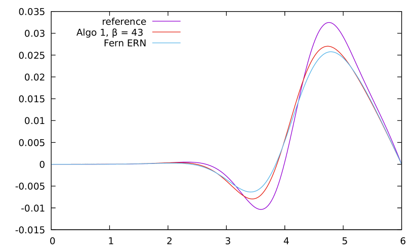
(b) rate = 3

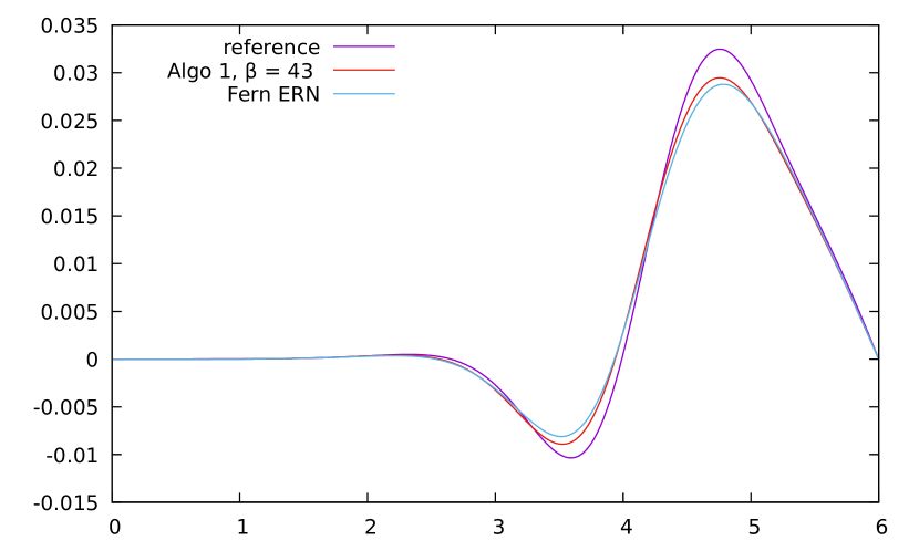
(c) rate = 4

(d) rate = 5

Figure 2: Structure displacement of Fernandez Explicit Robin-Neumann scheme (Fern ERN) and Algorithm 1 (Algo 1) with $\beta=43$ at final time

(a) rate = 2

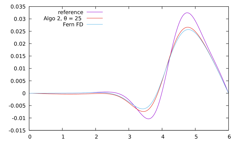
(b) rate = 3

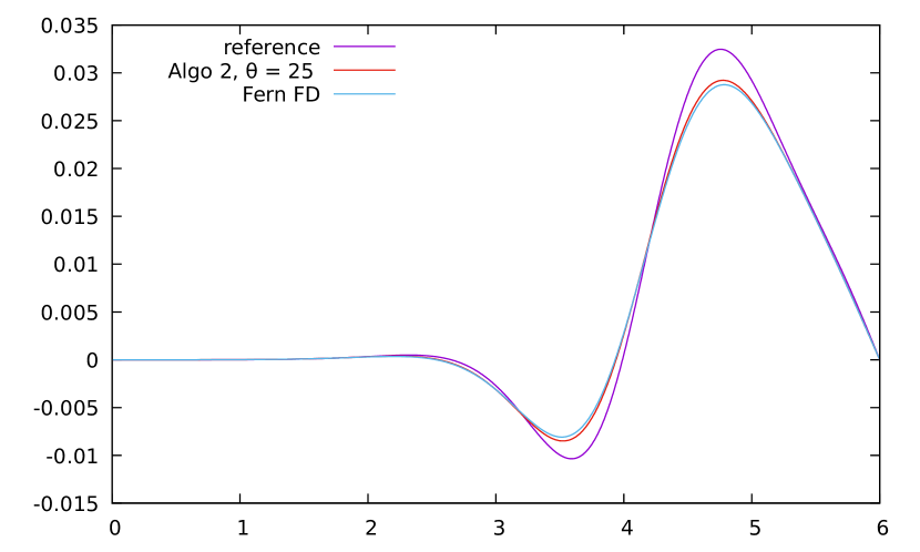
(c) rate = 4

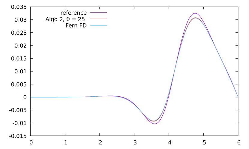
(d) rate = 5

Figure 3: Structure displacement of Fernandez fully decoupled scheme (Fern FD) and Algorithm 2 (Algo 2) with $\theta=25$ at final time

(a) rate = 2

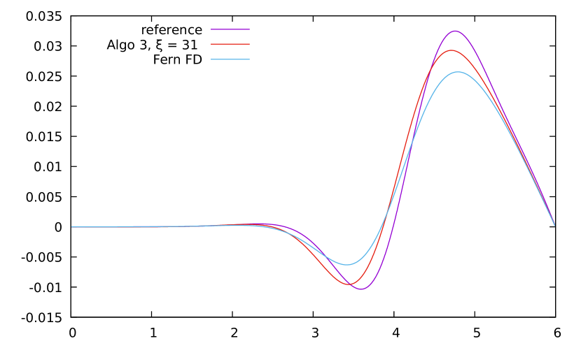
(b) rate = 3

(c) rate = 4

(d) rate = 5

Figure 4: Structure displacement of Fernandez fully decoupled scheme (Fern FD) and Algorithm 3 (Algo 3) with $\xi=31$ at final time

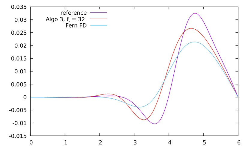
(a) rate = 2

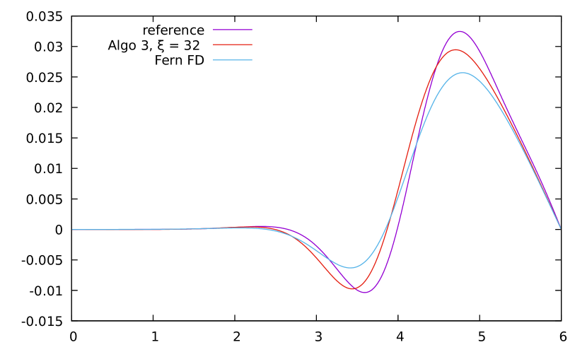
(b) rate = 3

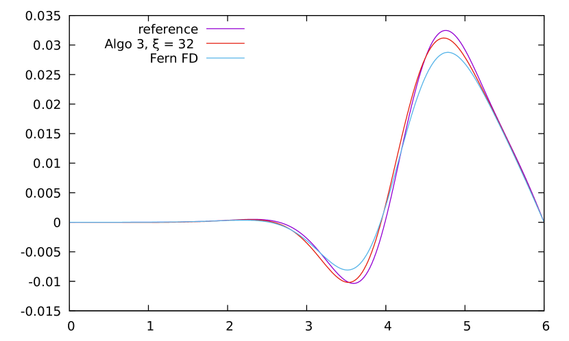
(c) rate = 4

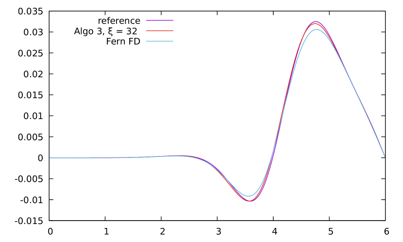
(d) rate = 5

Figure 5: Structure displacement of Fernandez fully decoupled scheme (Fern FD) and Algorithm 3 (Algo 3) with $\xi=32$ at final time

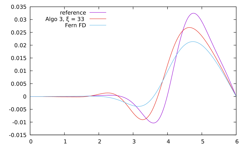
(a) rate = 2

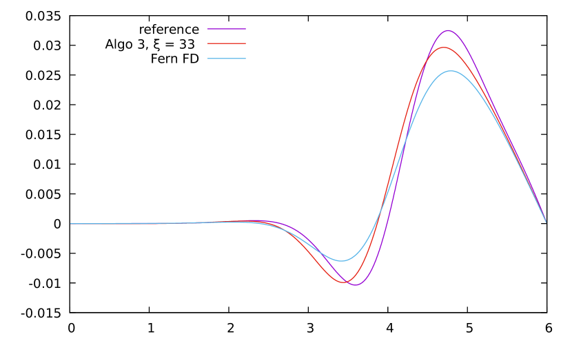
(b) rate = 3

(c) rate = 4

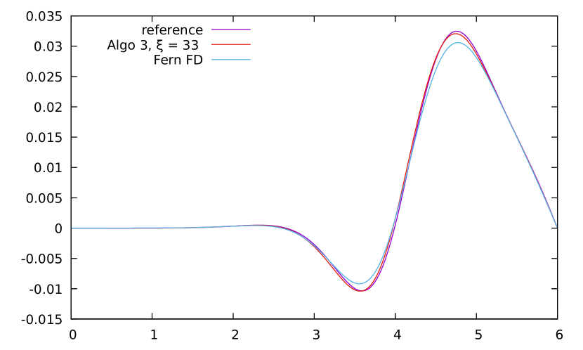
(d) rate = 5

Figure 6: Structure displacement of Fernandez fully decoupled scheme (Fern FD) and Algorithm 3 (Algo 3) with $\xi=33$ at final time

12 Discussions and future work

The numerical results validate the ideas that adding force corresponding to viscosity and replacing underlying projection method can improve accuracy; particularly, Table LABEL:table:prj_prs-coret_Van-Kan_m3_selected indicates as large improvement as up to $49.5229\%$ for Algorithm 3 with $\xi=33$ compared with Fernandez fully decoupled scheme at refinement $\textit{rate}=5$. It is expected, for other fluid-structure interaction problems, if the fluid is also viscous, adding force might also help with accuracy.

As a direction of future work, it is worth trying investigating how adding force improve accuracy theoretically. Reading some works on boundary layer theory might benefit such analysis.

This work deals with accuracy. On the other hand, it is possible to improve efficiency by parallelism. A choice is to take advantage of extrapolation ($1^{st}$ order might be better than $0^{th}$ ). To implement such ideas, MPI [3] might work.

13 Acknowledgments

This research did not receive any specific grant from funding agencies in the public, commercial, or not-for-profit sectors.

References

- [1] S. Abrate. 2 - dynamic behavior of composite marine propeller blades. In Valentina Lopresto, Antonio Langella, and Serge Abrate, editors, Dynamic Response and Failure of Composite Materials and Structures, pages 47 – 83. Woodhead Publishing, 2017.
- [2] Santiago Badia, Fabio Nobile, and Christian Vergara. Fluid–structure partitioned procedures based on robin transmission conditions. Journal of Computational Physics, 227(14):7027 – 7051, 2008.
- [3] Blaise Barney. Message passing interface (mpi). https://computing.llnl.gov/tutorials/mpi/. Accessed June 01 2019.
- [4] G. BIRKHOFF. Hydrodynamics. Princeton University Press, Princeton, 1960.
- [5] Pitkäranta J Brezzi F. On the stabilization of finite element approximations of the stokes equations. Efficient Solutions of Elliptic Systems (Kiel, 1984), Notes on Numerical Fluid Mechanics, 10:11–19, 1984.
- [6] Martina Bukač, Sunčica Čanić, Roland Glowinski, Josip Tambača, and Annalisa Quaini. Fluid–structure interaction in blood flow capturing non-zero longitudinal structure displacement. Journal of Computational Physics, 235:515 – 541, 2013.
- [7] Erik Burman and Miguel A. Fernández. Stabilization of explicit coupling in fluid–structure interaction involving fluid incompressibility. Computer Methods in Applied Mechanics and Engineering, 198(5):766 – 784, 2009.
- [8] P. Causin, J.F. Gerbeau, and F. Nobile. Added-mass effect in the design of partitioned algorithms for fluid–structure problems. Computer Methods in Applied Mechanics and Engineering, 194(42):4506 – 4527, 2005.
- [9] Miguel A. Fernandez. Fsi lectures tutorial 2: Robust and accurate splitting schemes. November 9-13, 2015, IST, Lisbon, Portugal.
- [10] Miguel Angel Fernández. Coupling schemes for incompressible fluid-structure interaction: implicit, semi-implicit and explicit. SeMA Journal: Boletin de la Sociedad Española de Matemática Aplicada, (55):59–108, June 2011.
- [11] M.A. Fernández and M. Landajuela. A fully decoupled scheme for the interaction of a thin-walled structure with an incompressible fluid. Comptes Rendus Mathematique, 351(3-4):161–164, 2013.
- [12] Miguel A. Fernández. Incremental displacement-correction schemes for the explicit coupling of a thin structure with an incompressible fluid. Comptes Rendus Mathematique, 349(7):473 – 477, 2011.
- [13] Miguel A. Fernández, Mikel Landajuela, and Marina Vidrascu. Fully decoupled time-marching schemes for incompressible fluid/thin-walled structure interaction. Journal of Computational Physics, 297(C):156–181, 2015.
- [14] Miguel A. Fernández, Jimmy Mullaert, and Marina Vidrascu. Explicit robin-neumann schemes for the coupling of incompressible fluids with thin-walled structures. Computer Methods in Applied Mechanics and Engineering, 267:566 – 593, 2013.
- [15] Luca Formaggia, Alfio Quarteroni, and Allesandro Veneziani. Cardiovascular Mathematics: Modeling and simulation of the circulatory system. Springer Milan : Imprint: Springer, Milano, 1st ed.. edition, 2009.
- [16] Brian Fox and Chet Ramey. Gnu bash. https://www.gnu.org/software/bash/. GNU Bash 4.4 August 26 2016.
- [17] Hassan Ghassemi and Ehsan Yari. The added mass coefficient computation of sphere, ellipsoid and marine propellers using boundary element method. Polish maritime research, 18(1):17–26, 2011.
- [18] J.L. Guermond, P. Minev, and Jie Shen. An overview of projection methods for incompressible flows. Computer Methods in Applied Mechanics and Engineering, 195(44-47):6011–6045, 2006.
- [19] Giovanna Guidoboni, Roland Glowinski, Nicola Cavallini, and Suncica Canic. Stable loosely-coupled-type algorithm for fluid–structure interaction in blood flow. Journal of Computational Physics, 228(18):6916 – 6937, 2009.
- [20] F. Hecht. New development in freefem++. J. Numer. Math., 20(3-4):251–265, 2012.
- [21] Alexandr I Korotkin. Added Masses of Ship Structures. Fluid Mechanics and Its Applications, 88. Springer Netherlands : Imprint: Springer, Dordrecht, 1st ed.. edition, 2009.
- [22] Dmitri Kuzmin. Operator splitting techniques. http://www.mathematik.uni-dortmund.de/~kuzmin/cfdintro/lecture11.pdf. Accessed August 1 2018.
- [23] G. LAMB. Hydrodynamics. Cambridge University Press, Cambridge, 1932.
- [24] A lot of contributors. Comprehensive perl archive network. https://www.cpan.org/. Accessed June 06 2020.
- [25] Mária Lukáčová-Medvid’ová, Gabriela Rusnáková, and Anna Hundertmark-Zaušková. Kinematic splitting algorithm for fluid–structure interaction in hemodynamics. Computer Methods in Applied Mechanics and Engineering, 265:83–106, 2013.
- [26] L Prandtl. On the motion of a fluid with very small viscosity verh. Int. Math. Kongr. 3rd. Heidelberg, pages 484–491, 1904.
- [27] Itiro Tani. History of boundary layer theory. Annual review of fluid mechanics, 9(1):87–111, 1977.
- [28] Linus Torvalds and a huge number of contributors. The linux kernel archives. https://www.kernel.org/. Accessed June 07 2020.
- [29] Larry Wall and the help of oodles of other folks. The perl programming language. https://www.perl.org/. Perl v5.30.0 April 17 2020.
- [30] Thomas Williams, Colin Kelley, and a large number of contributors on SourceForge. Gnuplot. http://www.gnuplot.info/. Gnuplot v5.0.16(1)-release (x86_64-pc-linux-gnu) 4th Berkeley Distribution March 15 2019.