Effective models and predictability of chaotic multiscale systems via machine learning

Abstract

Understanding and modeling the dynamics of multiscale systems is a problem of considerable interest both for theory and applications. For unavoidable practical reasons, in multiscale systems, there is the need to eliminate from the description the fast/small-scale degrees of freedom and thus build effective models for only the slow/large-scale degrees of freedom. When there is a wide scale separation between the degrees of freedom, asymptotic techniques, such as the adiabatic approximation, can be used for devising such effective models, while away from this limit there exist no systematic techniques. Here, we scrutinize the use of machine learning, based on reservoir computing, to build data-driven effective models of multiscale chaotic systems. We show that, for a wide scale separation, machine learning generates effective models akin to those obtained using multiscale asymptotic techniques and, remarkably, remains effective in predictability also when the scale separation is reduced. We also show that predictability can be improved by hybridizing the reservoir with an imperfect model.

I Introduction

Machine learning techniques are impacting science at an impressive pace from robotics [1] to genetics [2], medicine [3], and physics [4]. In physics, reservoir computing [5, 6], based on echo-state neural networks [7, 8, 9], is gathering much attention for model-free, data-driven predictions of chaotic evolutions [10, 11, 12, 13, 14]. Here, we scrutinize the use of reservoir computing to build effective models for predicting the slow degrees of freedom of multiscale chaotic systems. We also consider hybrid reservoirs, blending data with predictions based on an imperfect model [15] (see also Ref. [16]).

Multiscale chaotic systems represent a challenge to both theory and applications. For instance, turbulence can easily span over 4/6 decades in temporal/spatial scales [17], while climate time scales range from hours of atmosphere variability to thousands years of deep ocean currents [18, 19]. These huge ranges of scales stymie direct numerical approaches making modeling of fast degrees of freedom mandatory, being slow ones usually the most interesting to predict. In principle, the latter are easier to predict: the maximal Lyapunov exponent (of the order of the inverse of the fastest time scale) controls the early dynamics of very small perturbations appertaining to the fast degrees of freedom that saturate with time, letting the perturbations on the slow degrees of freedom to grow at a slower rate controlled by the typically weaker nonlinear instabilities [20, 21, 22]. However, owing to nonlinearity, fast degrees of freedom depend on, and in turn, impact on the slower ones. Consequently, improper modeling the former severely hampers the predictability of the latter [23].

We focus here on a simplified setting with only two time scales, i.e. on systems of the form:

$$\dot{\bm{X}} =\frac{1}{\tau_{s}}\bm{F}_{s}(\bm{X},\bm{x})$$ (1)

$$\dot{\bm{x}} =\frac{1}{\tau_{f}}\bm{F}_{f}(\bm{x},\bm{X})\,,$$

where $\bm{X}$ and $\bm{x}$ represent the slow and fast degrees of freedom, respectively. The time scale separation between them is controlled by $c\!=\!\tau_{s}/\tau_{f}$. The goal is to build an effective model for the slow variables, $\dot{\bm{X}}\!=\!\!\bm{F}_{\mathrm{eff}}(\bm{X})$, to predict their evolution. When the fast variables are much faster than the slow ones ($c\gg 1$), multiscale techniques [24, 25] can be used to build effective models. Aside from such limit, systematic methods for deriving effective models are typically unavailable.

In this article, we show that reservoir computers trained on time series of the slow degrees of freedom can be optimized to build (model-free data-driven) effective models able to predict the slow dynamics. Provided the reservoir dimensionality is high enough, the method works both when the scale separation is large, red basically recovering the results of standard multiscale methods, such as the adiabatic approximation, and when it not so large. Moreover, we show that even an imperfect knowledge of the slow dynamics can be used to improve predictability, also for smaller reservoirs.

The material is organized as follows. In Sec. II we present the reservoir computing approach for predicting chaotic systems, moreover we provide the basics of its implementation also considering the case in which an imperfect model is available (hybrid implementation). In Sec. III we present the main results obtained with a specific multiscale system. Section IV is devoted to discussions and perspectives. In Appendix A we give further details on implementation, including the choice of hyperparameters. Appendix B presents the adiabatic approximation for the multiscale system here considered. In Appendix C we discuss and compare different hybrid schemes.

II Reservoir computing for chaotic systems and its implementation

Reservoir computing [5, 6] is a brain inspired approach based on a recurrent neural network (RNN), the reservoir (R) – i.e. an auxiliary high dimensional nonlinear dynamical system naturally suited to deal with time sequences–, (usually) linearly coupled to a time dependent lower dimensional input (I), to produce an output (O). To make O optimized for approximating some desired dynamical observable, the network must be trained. Reservoir computing implementation avoids backpropagation [26] by only training the output layer, while R-to-R and I-to-R connections are quenched random variables. Remarkably, the reservoir computing approach allows for fast hardware implementations with a variety of nonlinear systems [27, 28]. Choosing the output as a linear projection of functions of the R-state, the optimization can be rapidly achieved via linear regression. The method works provided R-to-R connections are designed to force the R-state to only depend on the recent past history of the input signal, fading the memory of the initial state.

II.1 Predicting chaotic systems with reservoir computing

When considering a chaotic dynamical system with state $\bm{s}(t)=(\bm{X}(t),\bm{x}(t))$, with reference to Eqs. (1), the input signal $\bm{u}(t)\in\mathrm{I\!R}^{D_{I}}$ is typically a subset of the state observables, $\bm{u}(t)\!=\!\bm{h}(\bm{s}(t))$. For instance, in the following we consider functions of the slow variables, $\bm{X}$, only. When the dimensionality, $D_{R}$, of the reservoir is large enough and the R-to-R connections are suitable chosen, its state, $\bm{r}(t)\in\mathrm{I\!R}^{D_{R}}$, becomes a representation – an echo – of the input state $\bm{s}(t)$ [9, 6, 12], via a mechanism similar to generalized synchronization [12, 29]. In this configuration, dubbed open loop [30] (Fig. 1a), the RNN is driven by the input and, loosely speaking, synchronizes with it. When this is achieved, the output, $\bm{v}(t)\in\mathrm{I\!R}^{D_{O}}$ can be trained (optimized) to fit a desired function of $\bm{s}(t)$, for instance, to predict the next outcome of the observable, i.e. $\bm{v}(t+\Delta t)=\bm{u}(t+\Delta t)$. After training, we can close the loop by feeding the output as a new input to R (Fig. 1b), thus obtaining an effective model for predicting the time sequence. For the closed loop mode to constitute an effective (neural) model of the dynamics of interest, we ask the network to work for arbitrary initial conditions, i.e. not only right after the training: a property dubbed reusability in Ref.  [12]. For this purpose, when starting from a random reservoir state, a short synchronization period in open loop is needed before closing the loop. The method to work requires some stability property which cannot, in general, be granted in the closed loop configuration [30].

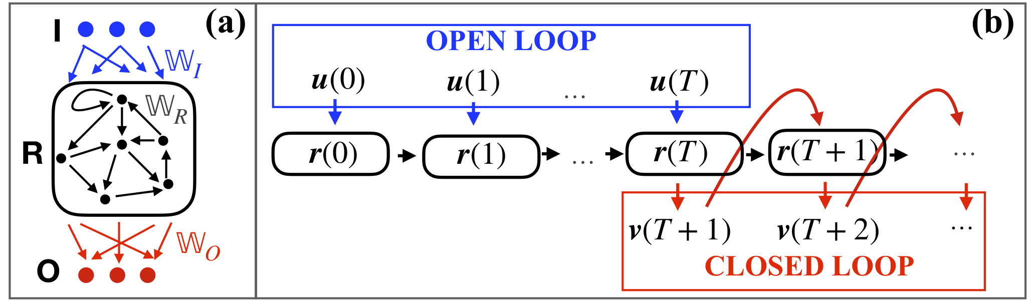
Figure 1: (Color online) Sketch of reservoir computing: (a) the components and their connections; (b) the two modes of operation: open loop for synchronizing the reservoir to the input and for training, closed loop for prediction.

II.2 Implementation

Reservoir neurons can be implemented in different ways [5], we use echo state neural network [9], mostly following [10, 11, 12]. Here, we assume $D_{R}\!\gg\!D_{I}\!=\!D_{O}$ and the input to be sampled at discrete time intervals $\Delta t$. Both assumptions are not restrictive, for instance in the hybrid implementation below we will use $D_{O}\neq D_{I}$ and the extension to continuous time is straightforward [5]. The reservoir is built via a sparse (low degree, $d$), random graph represented via a $D_{R}\times D_{R}$ connectivity matrix $\mathbb{W}_{R}$, with the non zero entries uniformly distributed in $[-1,\;1]$, scaled to have a specific spectral radius $\rho=\max\{|\mu_{i}|\}$ with $\mu_{i}$ being the matrix eigenvalues. The request $\rho<1$ is sufficient, though not strictly necessary [31], to ensure the echo state property [7, 8] in open loop, namely the synchronization of $\bm{r}(t)$ with $\bm{s}(t)$. We distinguish training and prediction. Training is done in open loop mode using an input trajectory $\bm{u}(t)$ with $t\in[-T_{s},T_{t}]$, where $T_{t}$ is the training input sequence length, and $T_{s}$ is the length of initial transient to let the $\bm{r}(t)$, randomly initialized at $t=-T_{s}$, to synchronize with the system dynamics. After being scaled to be zero mean and unit standard deviation, the input is linearly coupled to the reservoir nodes via a $D_{R}\times D_{I}$ matrix $\mathbb{W}_{I}$, with the non zero entries taken as random variables uniformly distributed in $[-\sigma,\;\sigma]$. In open loop mode the network state $\bm{r}(t)$ is updated as

$$\bm{r}(t+\Delta t)=\tanh[\mathbb{W}_{R}\bm{r}(t)+\mathbb{W}_{I}\bm{u}(t)]\,.$$ (2)

In the above expression the $\tanh$ is applied element wise, and can be replaced with other nonlinearities. The output is computed as $\bm{v}(t+\Delta t)=\mathbb{W}_{O}\bm{r}^{\star}(t+\Delta t)$ with the $D_{R}\times D_{O}$ matrix $\mathbb{W}_{O}$ obtained via linear regression by imposing $\mathbb{W}_{O}=\arg\min_{\mathbb{W}}\{\sum_{0\leq t\leq T_{t}}||\bm{v}(t)-\bm{u}(t)||^{2}+\alpha\mathrm{Tr}[\mathbb{W}\mathbb{W}^{T}]\}$, to ensure the output to be the best predictor of the next input observable. The term proportional to $\alpha$ is a regularization, while $\bm{r}^{\star}$ is a function of the reservoir state. Here, we take $r^{*}_{i}(t)=r_{i}(t)$ if $i$ is odd and $r^{*}_{i}(t)=r^{2}_{i}(t)$ otherwise [32]. Once $\mathbb{W}_{O}$ is determined, we switch to prediction mode. Given a short sequence of measurements, in open loop, we can synchronize the reservoir with the dynamics (2), and then close the loop letting $\bm{u}(t)\leftarrow\bm{v}(t)=\mathbb{W}_{O}\bm{r}^{\star}(t)$ in Eq. (2). This way Eq. (2) becomes a fully data-driven effective model for the time signal to be predicted. The resulting model, and thus its performances, will implicitly depend both on the hyperparameters ($d,\rho$ and $\sigma$) defining the RNN structure and the I-to-R connections and on the length of the training trajectory ($T_{t}$). The choices of these hyperparameters are discussed in Appendix A.

II.3 Hybrid implementation

So far we assumed no prior knowledge of the dynamical system that generated the input. If we have an imperfect model for approximately predicting the next outcome of the observables $\bm{u}(t)$, we can include such information in a hybrid scheme by slightly changing the input and/or output scheme to exploit this extra knowledge [15, 16]. The idea of blending machine learning algorithms with physics informed model is quite general and it has been exploited also with methods different from reservoir computing, see e.g. Refs. [33, 34, 35].

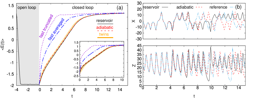
Figure 2: (Color online) Prediction error growth for a single realization of a network of $D_{R}\!=\!500$ neurons. (a) Average (over $10^{4}$ initial conditions) ($\log_{10}$)error $\langle E(t)\rangle$ vs time during synchronization (open loop, gray region) and prediction (closed loop) for $c\!=\!10$ and $\Delta t\!=\!0.1$: the yellow shaded area circumscribes the twin and random twin model predictions (see text); reservoir computer prediction (solid, black curve) compared with that of the truncated model (purple, dotted curve), of the model fast variables replaced by their average (blue, dash dotted curve) and model (11) (red, dashed curve). The inset shows the same (closed loop only) for $\Delta t\!=\!0.01$. (b) An instance of a prediction experiment, showing the reference (dash dotted, light blue curves) evolution of the $X$ (top) and $Z$ (bottom) variables of the coupled Lorenz model (6) together with the prediction obtained via the reservoir (black, solid curve) and the adiabatic model (dashed, red curve). For details on hyperparameters see Appendix A.6.

Let $\wp[\bm{u}(t)]=\hat{\bm{u}}(t+\Delta t)$ be the estimated next outcome of the observable $\bm{u}(t)$ according to our imperfect model. The idea is to supply such information in the input by replacing $\bm{u}(t)$ with the column vector $(\bm{u}(t),\wp[\bm{u}(t)])^{T}$, thus doubling the dimensionality of the input matrix. For the output we proceed as before. The whole scheme is thus as the above one with the only difference that $\mathbb{W}_{O}$ is now a $D_{R}\times D_{I}/2$. The switch to the prediction mode is then obtained using $(\mathbb{W}_{O}\bm{r}^{\star}(t),\wp[\mathbb{W}_{O}\bm{r}^{\star}(t)])^{T}$ as input in Eq. (2).

It is worth noticing that other hybrid schemes are possible, e.g. in Ref. [15] the output has the form $\bm{v}(t+\Delta t)=\mathbb{W}_{O}(\bm{r}^{\star}(t),\wp[\bm{u}(t)])^{T}$, namely a combination of the prediction based on the network and on the physical model. In Appendix C we comment further on our choice, and we compare it with the scheme proposed in Ref. [15].

III Results for a two time scales system

We now consider the model introduced in Ref. [36] as a caricature for the interaction of the (fast) atmosphere and the (slow) ocean. It consists of two Lorenz systems coupled as follows:

$$\left\{\begin{array}[]{l}\dot{X}=a(Y-X)\\ \dot{Y}=R_{s}X-ZX-Y-\epsilon_{s}xy\\ \dot{Z}=XY-bZ\end{array}\right.$$ (6)

$$\left\{\begin{array}[]{ll}\dot{x}=ca(y-x)\\ \dot{y}=c(R_{f}x-zx-y)+\epsilon_{f}Yx\\ \dot{z}=c(xy-bz)\,,\end{array}\right.$$ (10)

where Eqs. (6) and Eqs. (10) describe the evolution of the slow and fast variables, respectively. We fix the parameters as in Ref. [36]: $a=10$, $b\!=\!8/3$, $R_{s}\!=\!28$, $R_{f}\!=\!45$, $\epsilon_{s}\!=\!10^{-2}$ and $\epsilon_{f}\!=\!10$, while for the time scale separation parameter, $c$, we use $c\!=\!10$ (as in Ref. [36]) and $c\!=\!3$. The former corresponds to a scale separation such that the adiabatic approximation already provides good results (see below). Moreover, for $c\!=\!10$, the error growth on the slow variables is characterized by two exponential regimes [36]: the former with rate given by the Lyapunov exponent of the full system $\lambda_{f}\!\approx\!11.5$, and the latter by $\lambda_{s}\!\approx\!0.85$, controlled by the fast and slow instabilities, respectively. This decomposition can be made more rigorous as shown in Ref. [37] for a closely related model.

We test the reservoir computing approach inputting the slow variables, i.e. $\bm{u}(t)\!=\!(X(t),Y(t),Z(t))$. In open loop, we let the reservoir to synchronize with the input, subsequently we perform the training and optimize $\mathbb{W}_{O}$ as explained earlier. Then, to test the prediction performance we consider $10^{4}$ initial conditions, for each of which, we feed the slow variables to the network in open loop and record, from $t\!=\!-T_{s}$ to $t\!=\!0$, the one step ($\log_{10}$)error $E(t)\!=\!\log_{10}\|{\bm{v}}(t)-{\bm{u}}(t)\|$, ${\bm{v}}(t)$ being the one-step network forecast (output).

Initially, the average ($\log_{10}$)error $\langle E(t)\rangle$ decreases linearly as shown in the grey regions of Figs. 2a and 3a, which is a visual proof of the echo state property. Then, it reaches a plateau - the synchronization error $E_{S}$ - which can be interpreted as the average smallest ($\log_{10}$)error on the initial condition and the one step error prediction.

At the end of the open loop, after synchronization, we switch to the prediction (closed loop) configuration and compute the ($\log_{10}$)error growth between the network prediction and the reference trajectory. Moreover, we take the output variables at the end of the open loop and use them as initial conditions for other models (discussed below) which are used as a comparison. First, we consider the perfect model with an error on the initial condition, i.e Eqs. (6) with the slow variables set equal to the network-obtained values at $t=0$, i.e. at the end of the open loop. By construction, the network does not forecast the fast variables, which are thus initialized either using their exact values from the reference trajectory (twin model), which is quite “unfair”, or random values (random twin) from the stationary measure on the fast attractor with fixed slow variables. Then we consider increasingly refined effective models for the slow degrees of freedom only: a “truncated” model, $\dot{\bm{X}}\!=\!\bm{F}_{T}(\bm{X})$, obtained from Eqs. (6) by setting $\epsilon_{s}\!=\!0$; a model in which we replace the fast variables in Eqs. (6) with their global average; the adiabatic model in which fast variables are averaged with fixed slow variables, which amounts to replacing $\epsilon_{s}xy$ in the equation for $\dot{Y}$ with (see Appendix B for details on the derivation):

$$\epsilon_{s}\langle xy\rangle_{\bm{X}}\!=\!(1.07\!+\!0.26Y/c)\,\Theta(\!1.07\!+\!0.26Y/c)\,,$$ (11)

where $\Theta$ denotes the Heaviside step function.

In Fig. 2 we show the results of the comparison between the prediction obtained with the reservoir computing approach and the different models above described for $c=10$, with sampling time $\Delta t=0.1$ (and $\Delta t=0.01$ in the inset of Fig. 2a). Figure 2a shows that eliminating the fast degrees of freedom (truncated model) or just considering their average effect leads to very poor predictions, while the prediction of the reservoir computer is comparable to that of the adiabatic model (11), as qualitatively shown in Fig. 2b (whose top/bottom panels show the evolution of the slow variables $X$ and $Z$ for the reference trajectory and the predictions obtained via the reservoir and adiabatic model). Remarkably, the reservoir-based model seems to even slightly outperform the twin model. A fact we understand as follows: by omitting fast components, one does not add fast decorrelating fluctuations to those intrinsic to the reference trajectories, thus reducing effective noise. Notice that the zero error on fast components of the twin model is rapidly pushed to its saturation value by the error on the slow variables. The sampling time $\Delta t\!=\!0.1$ is likely playing an important role during learning by acting as a low passing filter. Indeed the comparison with twin model slightly deteriorates for $\Delta t\!=\!0.01$ (see Fig. 2a inset).

Figure 3 shows the results for $c\!=\!3$. Here, the poor scale separation spoils the effectiveness of the adiabatic model (11) while the prediction obtained via the reservoir computing approach remains effective, as visually exemplified in Fig. 3b and quantified in Fig. 3a. Notice that, however, the network predictability deteriorates with respect to the previous case and the twin model does better, though the reservoir still outperforms the random twin model. This slight worsening is likely due to the fact that discarded variables are not fast enough to average themselves out, making the learning task harder. Nevertheless, the network remains predictive.

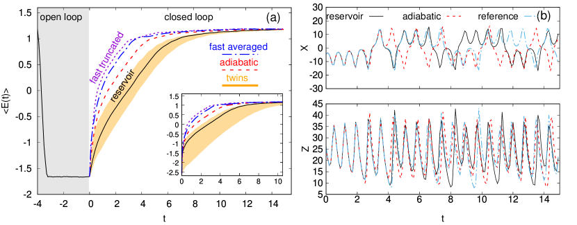
Figure 3: (Color online) Same as Fig. 2 for the case $c=3$.

III.1 Which effective model the network has built?

We now focus on the case $c\!=\!10$ and $\Delta t\!=\!0.01$, for which we can gain some insights into how the network works by comparing it to the adiabatic model (11). The sampling time is indeed small enough for time differences to approximate derivatives. In Fig. 4 we demonstrate that the network in fact generates an effective model akin to the adiabatic one (11). Here we show a surrogate of the residual time derivative of $Y$, meaning that we removed the truncated model derivative, as a function of $Y$:

$$\Delta\widetilde{\dot{Y}}=\frac{Y(t+\Delta t)-Y(t)}{\Delta t}-\frac{Y_{T}(t+\Delta t)-Y(t)}{\Delta t}\,,$$ (12)

The expression in Eq. (12) provides a proxy for how the network has modeled the term $-\epsilon_{s}xy$ in Eqs. (6). The underlying idea is as follows. We let the network evolve in closed loop, at time $t$ it takes as input the forecasted slow variables $\bm{v}(t)\!=\!(\hat{X}(t),\hat{Y}(t),\hat{Z}(t))$ and it outputs the next step forecast $\bm{v}(t\!+\!\Delta t)\!=\!(\hat{X}(t\!+\!\Delta t),\hat{Y}(t\!+\!\Delta t),\hat{Z}(t\!+\!\Delta t))$. We then use $\bm{v}(t)$ as input to the truncated model, and evolve it for a time step $\Delta t$ to obtain $(X_{T}(t+\Delta t),Y_{T}(t+\Delta t),Z_{T}(t+\Delta t))$. Equation (12) is then used to infer how the network models the coupling with the fast variables. Evolving by one time step $\bm{v}(t)$ using Eqs. (11) and then again employing (12) we, obviously, obtain the line $-1.07-0.26Y$ (dashed in Fig. 2c). The network residual derivatives (black dots in Fig. 4) distribute on a narrow stripe around that line. This means that the network, for wide scale separation, performs an average conditioned on the values of the slow variables. For $c=10$, such conditional average is equivalent to the adiabatic approximation (11), as discussed in Appendix B. For comparison, we also show the residual derivatives (12) computed with the full model (6-10) (gray dots), which display a scattered distribution, best fitted by Eq. (11). For $c=3$, while the adiabatic approximation is too rough, remarkably the network still performs well even though is more difficult to identify the model it has build, which will depend on the whole set of slow variables (see Appendix B for a further discussion).

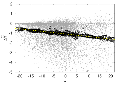
Figure 4: (Color online) Residual derivatives (12) vs $Y$ for $c\!=\!10$ and $\Delta t\!=\!0.01$, computed with the network (black dots), the multiscale model (11) (yellow, dashed line), and the full dynamics (gray dots). For details on hyperparameters see Appendix A.6.

III.2 Predictability time and hybrid scheme

So far we focused on the predictability of a quite large network ($D_{R}\!=\!500$ as compared to the low dimensionality of Eqs. (6-10)). How does the network performances depend on the reservoir size $D_{R}$?

In Fig. 5 we show the $D_{R}$-dependence of the average (over reservoir realizations and initial conditions) predictability time, $T_{p}$, defined as the first time such that the error between the network predicted and reference trajectory reaches the threshold value $\Delta^{*}=0.4\langle||\bm{X}||^{2}\rangle^{1/2}$. For $D_{R}\gtrsim 450$, the predictability time saturates while for smaller reservoirs it can be about threefold smaller and, in addition, with large fluctuations mainly due to unsuccessful predictions, i.e. instances in which the network is unable to proper modeling the dynamics (see Fig 6). Remarkably, implementing the hybrid scheme even with a poorly performing predictor such as the truncated model, the forecasting ability of the network improves considerably (as also shown in Fig. 5). In particular, with the hybrid scheme, saturation is reached earlier (for $D_{R}\gtrsim 300$) and, for smaller reservoirs, the predictability time of the hybrid scheme is longer. Moreover, the hybrid scheme is less prone to failures even for small $D_{R}$, hence fluctuations are smaller (see Fig. 6). Note that the chosen hybrid design ensures that the improvement is only due to reservoir capability of building a better effective model, reducing the average synchronization ($\log_{10}$)error $\langle E_{S}\rangle$ (see the insets of Fig. 5 and 6, and the discussion in Appendix C) and thus the error on the initial condition of the slow variables. Indeed, in the inset of Fig. 5 we also show the slope predicted on the basis of the slow perturbation growth rate, $\lambda_{s}$ [36].

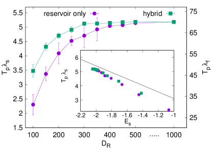
Figure 5: (Color online) Average predictability time, $T_{p}$ normalized with the slow finite size Lyapunov exponent $\lambda_{s}$ (left scale) and with the (fast) maximal Lyapunov exponent $\lambda_{f}$ (right scale), versus reservoir size $D_{R}$ (hyperparameters for the hybrid implementation are the same of the reservoir only approach which are discussed in Appendix A.6) for reservoir only (purple circles) and hybrid scheme (green squares), system parameters $c\!=\!10$ and $\Delta t\!=\!0.1$. Error bars denote statistical standard deviation over 20 independent network realizations, each sampling $10^{3}$ initial conditions. Inset: $T_{p}\lambda_{s}$ vs synchronization average ($\log_{10}$)error $\langle E_{S}\rangle$. The slope of the black line is $-1$ corresponding to the slow perturbation growth rate $\lambda_{s}$.

The above observations boil down to the fact that the difference between hybrid and reservoir only approach disappears at increasing $D_{R}$ as the same plateau values for both synchronization error and predictability time are reached. In other terms, if the reservoir is large enough, adding the extra information from the imperfect model does not improve the model produced by the network. These conclusions can be cast in a positive message by saying that using a physically informed model allows for reducing the size of the reservoir to achieve a reasonable predictability and hence an effective model of the dynamics with a smaller network, which is important when considering multiscale systems of high dimensionality.

We remark that in Fig. 5 the predictability time $T_{p}$ was made nondimensional either using the growth rate of the slow dynamics $\lambda_{s}$ (left scale of Fig. 5), or using the Lyapunov exponent $\lambda_{f}$ of the full system (right scale) which is dominated by the fast dynamics. For large networks the predictability time is as large as $5$ (finite size) Lyapunov times, which corresponds to about $70$ Lyapunov times with respect to the full dynamics. Such a remarkably long predictability with respect to the fastest time scale is typical of multiscale systems, where the maximal Lyapunov exponent does not say much for the predictability of the slow degrees of freedom [20, 21, 22].

Figures 2a, 3a and 5(inset) (see also the inset of Fig. 6), show that it is hard reaching synchronization error below $10^{-2}$. Even when this happens it does not improve the predictability, as the error quickly (even faster than the Lyapunov time) raises to values $O(10^{-2})$. Indeed, such an error threshold corresponds to the crossover scale between the fast- and slow-controlled regime of the perturbation growth (see Fig. 2 in Ref. [36]). In other terms, pushing the error below this value requires the reservoir to (partially) reconstruct also the fast component dynamics.

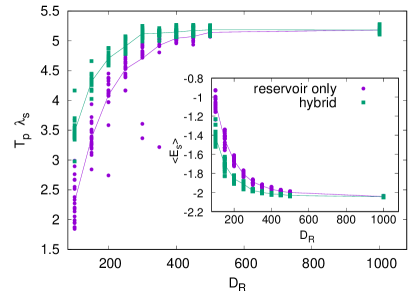
Figure 6: (Color online) Nondimensional predictability time $T_{p}\lambda_{s}$ of $20$ network realizations (each averaged over $10^{4}$ initial conditions), in reservoir only (purple circles) and hybrid scheme (green squares), as a function of the reservoir size $D_{R}$. The solid curves display the average over all realizations, already presented in Fig. 3. Notice that, in the reservoir only scheme, a number of outliers are present for $D_{R}\lesssim 400$, these correspond to “failed” networks that make poor medium term predictions or even fail to reproduce the climate. Remarkably, such failures are not observed in the hybrid scheme. Inset: $\langle E_{S}\rangle$, i.e. the average (over network realizations and $10^{4}$ initial conditions for each realizations) ($\log_{10}$)error at the end of the open loop versus the reservoir size $D_{R}$ for the reservoir only (purple curve) and the hybrid (green curve) scheme, respectively. Symbols display the synchronization error in each network realization. Notice that there are no realizations with strong departure from the average as observed in main panel for the predictability time: this shows that the predictability performance is not always liked to the synchronization error (see text for a further discussion). Data refer to the case $c=10$ and $\Delta t=0.1$. For hyperparameters see Appendix A.6.

III.3 The role of the synchronization error

In the previous section, we have used the average predictability time, $T_{p}$, as a performance metrics. If we interpret the synchronization error (at the end of the open loop) as the error on the initial conditions, since the system is chaotic, we could naively think that reducing such error always enhances the predictability. Consequently, one can expect the size of such error to be another good performance metrics. In the following, we show that this is only partially true.

Obviously, to achieve long term predictability the smallness of the synchronization error is a necessary condition. Indeed the (log)error at the end of open loop cycle, $E_{S}$, puts an upper limit to the predictability time as

$$T_{p}\lesssim\frac{1}{\lambda_{s}}[\log(\Delta^{*})-E_{S}]\,,$$ (13)

as confirmed by the solid line in the inset of Fig. 5. However, it is not otherwise very informative about the overall performance. The reason is that the value of $E_{S},$ which can also be seen as the average error on one step predictions, does not provide information on the structural stability of the dynamics. Indeed, for a variety of hyperparameters values, we have observed low $E_{S}$ resulting in failed predictions: in other terms the model built by the network is not effective in forecasting and in reproducing the climate. In these cases, the network was unable to generate a good effective model, as shown in Fig. 6: this typically happens for relatively small $D_{R}$ in the reservoir only implementation.

In a less extreme scenario, the error $E_{S}$ can be deceptively lower than the scale at which the dynamics has been properly reconstructed. This latter case is relevant to the multiscale setting since, as outlined at the end of the previous section, fast variable reconstruction is necessary to push the initial error below a certain threshold. In some cases, we did observe the synchronization error falling below the typical value $10^{-2}$ but immediately jumping back to it, implying unstable fast scale reconstruction (for instance, see $c=3$, $\Delta t=0.01$ in Fig. 3a).

As a consequence of the two above observations, $E_{S}$ is an unreliable metric for hyperparameters landscape exploration as well. We also remark that, even if fast scales were modeled with proper architecture and training time, and $E_{S}$ could be pushed below the crossover with an actual boost in performance, such improvements would not dramatically increase the predictability time of the slow variables, since they are suppressed by the global (and greater, as dominated by the fast degrees of freedom) Lyapunov exponent. This situation as discussed above is typical of multiscale systems.

IV Conclusions

We have shown that reservoir computing is a promising machine learning tool for building effective, data-driven models for multiscale chaotic systems able to provide, in some cases, predictions as good as those that can be obtained with a perfect model with error on the initial conditions. Moreover, the simplicity of the system allowed us to gain insights into the inner work of the reservoir computing approach that, at least for large scale separation, is building an effective model akin to that obtained by asymptotic multiscale techniques. Finally, the reservoir computing approach can be reinforced by blending it with an imperfect predictor, making it to perform well also with smaller reservoirs. While we have obtained these results with a relatively simple two-timescale model, given the success of previous applications to spatially extended systems [11], we think the method should work also with more complex high dimensional multiscale systems. In the latter, it may be necessary to consider multi reservoir architectures [38] in parallel [11]. Moreover, reservoir computing can be used to directly predict unobserved degrees of freedom [39]. Using this scheme and the ideas developed in this work it would be interesting to explore the possibility to build novel subgrid schemes for turbulent flows [40, 41] (see also Ref. [16] for a very recent attempt in this direction based on reservoir computing with hybrid implementation), preliminary tests could be performed in shell models for turbulence for which physics only informed approaches have been only partially successful [42].

Appendix A Details on the implementation

A.1 Intra-reservoir (R-to-R) connectivity matrix $\mathbb{W}_{R}$

The intra-reservoir connectivity matrix, $\mathbb{W}_{R}$, is generated by drawing each entry from the same distribution. Each element is the product of two random variables $\mathbb{W}_{ij}=a*b\,$: $a$ being a real uniformly distributed random number in $[-1,\;1]$ and $b$ taking values $1$ or $0$ with probability $P_{d}=d/D_{R}$ and $1-P_{d}$, respectively. Consequently, each row has, on average, $d$ non zero elements. Since $D_{R}\gg d$, the number of non null entries per row is essentially distributed according to a Poisson distribution. As a last step, the maximal eigenvalue (in absolute value), $\rho_{\mathrm{max}}(\mathbb{W})$ of the resulting matrix $\mathbb{W}$ is computed and the matrix is rescaled element wise so that its new spectral radius matches the target value $\rho$, i.e.:

$$\mathbb{W}_{R}=\mathbb{W}\frac{\rho}{\rho_{\mathrm{max}}(\mathbb{W})}$$

A.2 Input-to-reservoir (I-to-R) connectivity matrix $\mathbb{W}_{I}$

The input to reservoir matrix $\mathbb{W}_{I}$ is generated in such a way that each reservoir node is connected to a single input. For this purpose, for each row $j$, a single element $n_{j}$, uniformly chosen between $1$ and the input dimension $D_{I}$, is different from zero. This means that the reservoir node $j$ is only connected to the $n_{j}^{th}$ input node. The connection strength is randomly chosen in $[-\sigma,\sigma]$ with uniform distribution.

A.3 Optimization of the output matrix $\mathbb{W}_{O}$

The output matrix $\mathbb{W}_{O}$ is obtained via optimization. As explained in Sec. II.2, $\mathbb{W}_{O}$ should be chosen so that the output $\bm{v}(t)=\mathbb{W}_{O}\,\bm{r}^{*}(t)$ is, on average, as similar as possible to the input signal $\bm{u}(t)$. Incidentally, we remark that the use of $\bm{r}^{*}$ instead of simply $\bm{r}$ is relevant to achieve accurate forecasting and is heuristically motivated by the need to add some nonlinearity in the network [7]. The particular choice we adopted, $r^{*}_{i}=r_{i}$ or $r_{i}^{2}$ for $i$ odd or even, respectively was suggested in Refs. [10, 12] in view of the symmetries of the Lorenz model.

As for the optimization of $\mathbb{W}_{O}$, we require that it should minimize the cost function

$$\mathcal{L}=\frac{1}{T_{t}}\sum_{0\leq t\leq T_{t}}\|\mathbb{W}_{O}\,r^{*}(t)-u(t)\|^{2}+\alpha\,\mbox{tr}[\mathbb{W}_{O}\,\mathbb{W}_{O}^{T}]\,,$$ (14)

where ^T denotes the transpose and $T_{t}$ is the length of the training input, whose choice is discussed below. We point out that the sum appearing in Eq. (14) is a delicate quantity: we have observed that moderate errors compromise the final performance. For this reason, the Kahan summation has been employed in order to boost numerical accuracy. The solution of the minimization of Eq. (14),

$$\mathbb{W}^{opt}_{O}\mbox{ so that }\left.\frac{d\mathcal{L}}{d\mathbb{W}_{O}^{T}}\right|_{\mathbb{W}^{opt}_{O}}=0$$

is

$$\mathbb{W}^{opt}_{O}=\langle u\otimes r^{*T}\rangle\;(\alpha\,\mathbb{I}_{D_{R}}+\langle r^{*}\otimes r^{*T}\rangle)^{-1}$$

where $\langle\cdot\rangle$ denotes the empirical average $\frac{1}{T_{t}}\sum_{t}$, $\otimes$ denotes the outer product and $\mathbb{I}_{D_{R}}$ the $D_{R}\times D_{R}$ identity matrix. The addend proportional to $\alpha$ in Eq. (14) is the Tikhonov term, which is a $L^{2}$ regularization on $\mathbb{W}_{O}$. The Tikhonov regularization improves the numerical stability of the inversion, which could be critical if the ratio between the largest and the smallest eigenvalues, $\rho_{\mathrm{max}}$ and $\rho_{\mathrm{min}}$, is too large and the latter would behave as a (numerical) null eigenvalue [43], as it is the case for the dynamics we are studying. Here we have used $\alpha=10^{-8.5}$ which empirically was found to lead to $\log_{10}(\rho_{\mathrm{max}}/\rho_{\mathrm{min}})\approx 10$.

A.4 Synchronization time and length of the training input trajectory

All results presented in this article have been obtained using training trajectories of length $T_{t}=500$. We remark that using values $100\leq T_{t}\leq 1000$ one can hardly notice qualitative differences. At low training times, failures can be very diverse, ranging from tilted attractors to periodic orbits or spurious fixed points. The chosen values of $T_{t}$ have been tested to be in the range that guarantees long term reconstruction of the attractor with proper hyperparameters. As for the the synchronizing length, we have chosen $T_{s}=4$. Such value is about four times larger than the time actually needed to achieve best possible synchronization indeed, as shown in the gray shaded areas of Figs. 2a and 3a, the error $E$ saturates to $E_{S}$ in about a time unit.

A.5 Numerical details

The whole code has been implemented in python3, with linear algebra performed via numpy. Numerical integration of the coupled Lorenz model were performed via a $4^{th}$ order Runge Kutta scheme.

A.6 Fixing the hyperparameters

The architecture of a generic network is described by a number of parameters, often dubbed hyperparameters, e.g.: the number of layers, activation functions etc. While a proper design is always crucial, in the reservoir computing paradigm, this issue is especially critical due to the absence of global optimization via backpropagation. The reservoir-to-reservoir and input-to-reservoir connectivity matrices, as discussed above, are quenched stochastic variables, whose distribution depends on four hyperparameters:

$$\mbox{Net}\sim P(\sigma,\rho,d,D_{R})\,,$$

namely, the strength of the I-to-R connection matrix $\sigma$, the spectral radius $\rho$ of the R-to-R connection matrix, the degree $d$ of the R-to-R connection graph, and the reservoir size $D_{R}$. Once the distribution is chosen, there are two separate issues.

The first is that, for a given choice of $(\sigma,\rho,d)$, the network should be self-averaging if its size $D_{R}$ is large enough. Indeed, we see from Fig. 6 that the variability between realizations decreases with $D_{R}$, as expected.

The second issue is the choice of the triple $(\sigma,\rho,d)$. In general, the existence of large and nearly flat (for any reasonable performance metrics) region of suitable hyperparameters implies the robustness of the method. As for the problem we have presented, such region exists, even though, in the case $\Delta t=0.1$, $c=10$, moderate fine tuning of the hyperparameters did improve the final result, allowing to even (moderately) outperform the fully informed twin model, as shown in Fig. 2a.

Figure 7: (Color online) Performance grid for $c=3$, $\Delta t=0.1$, $N=350$, $d=5$. Colors code error between forecasted and reference trajectory at time $t=5$ after closing the loop, which if the metrics here used $f=\|\bm{X}^{forecast}(t=5)-\bm{X}^{true}(t=5)\|$ (averaged over 100 points of the attractor) for a single realization of the network for a given value of parameters $(\rho,\sigma)$. To highlight the suitable parameter region, a cutoff on has been put at $f=1$.

It is important to remark that the characteristics of the regions of suitable hyperparameters depend on the used metric. Here, we have focused on medium term predictability, i.e. we evaluate the error between forecasted and reference slow variables at a time (after synchronization) that is much larger than one step $\Delta t$ but before error saturation (corresponding to trajectories completely uncorrelated). Requiring a too short time predictability, as discussed in Ref. [12], typically is not enough for reproducing long time statistical properties of the target system (i.e. the so called climate), as the learned attractor may be unstable even if the dynamical equations are locally well approximated. If both short term predictability and climate reproduction are required, the suitable hyperparameter region typically shrinks. The metric we used typically led to both predictability and climate reproduction, at least for reservoir sizes large enough.

In order to fix the parameters, two techniques have been employed. The first is the standard search on a grid (for a representative example see Fig. 7): a lattice is generated in the space of parameters, then each node is evaluated according to some cost function metrics. If such function is regular enough, it should be possible to detect a suitable region of parameters. While this default method is sound, it may require to train many independent networks, even in poorly performing regions. Each network cannot be too small for two reasons: the first is that small networks suffer from higher inter realization fluctuations, the second is that we cannot exclude that optimal $(\sigma,\rho,d)$ have a loose dependence on the reservoir size $D_{R}$. As further discussed below we found a mild dependence on the network degree $d$, provided it is not too large, thus in Fig.7 we focused on the dependence on $\rho$ and $\sigma$.

The second technique is the no gradient optimization method known as particle swarming optimization (PSO) [44]. PSO consists in generating $n$ (we used $n=10$) tuples of candidate – the particles – parameters, say ${\bf p}_{i}=(\rho_{i},\sigma_{i},d_{i})\;i=1,...,n$. At each step, each candidate is tested with a given metrics $f$. Here, we used the average (over $50-100$ initial conditions) error on the slow variables after $t=2,4,5$ (depending on the parameters) in the close loop configuration. Then, at each iteration $k$ of the algorithm, each candidate is accelerated towards a stochastic mixture of its own best performing past position

$${\bf p}_{i}^{*}(k)=\arg\min_{{\bf p}_{i}(s)}\{f({\bf p}_{i}(s))|s<k\}$$

and the overall best past performer

$${\bf p}^{*}(k)=\arg\min_{{{\bf p}_{i}^{*}}(k)}\{f({{\bf p}_{i}^{*}}(k))|i=1,...,n\}.$$

Particles are evolved with the following second order time discrete dynamics

$${\bf p}_{i}(k+1) = {\bf p}_{i}(k)+{\bf v}_{i}(k)$$

$${\bf v}_{i}(k+1) = w{\bf v}_{i}(k)+\phi^{1}_{i}(k)\,({\bf p}_{i}^{*}(k)-{\bf p}_{i}(k))$$

$$+ \phi^{2}_{i}(k)\,({\bf p}^{*}(k)-{\bf p}_{i}(k))$$

with $\phi_{i}^{j}(k)\in[0,1]$ being random variables and $w\in[0,1]$ representing a form of inertia, as implemented in the python library pyswarms. After a suitable amount of iterations, ${\bf p}^{*}$ should be a valid candidate. The advantage of PSO is that, after a transient, most candidate evaluations (each of which require to initialize, train and test at least one network) should happen in the good regions. It is worth pointing out that, unless self-averaging is achieved thanks to large enough reservoir sizes, inter network variability adds noise to limited attractor sampling when evaluating $f$ and, therefore, fluctuations may appear and trap the algorithm in suboptimal regions for some time. Moreover, the algorithm itself depends on some hyperparameters that may have to be optimized themselves by hand.

In our study, PSO has been mainly useful in fixing parameters in the ($\Delta t=0.1$, $c=10$) case and to observe that $d$ is the parameter which affects the performance the least. Some gridding (especially in $\rho$ and $\sigma$) around the optimal solution is useful, in general, as a cross check and to highlight the robustness (or lack thereof) of the solution.

In Table 1 we summarize the hyperparameters used in our study.

	$\Delta t=0.1$	$\Delta t=0.01$
c=3	$\begin{matrix}d=5\\ \sigma=2\\ \rho=0.35\end{matrix}$	$\begin{matrix}d=5\\ \sigma=2.5\\ \rho=0.25\end{matrix}$
c=10	$\begin{matrix}d=5\\ \sigma=1.8\\ \rho=0.34\end{matrix}$	$\begin{matrix}d=5\\ \sigma=0.8\\ \rho=0.68\end{matrix}$

Table 1: (Color online) Hyperparameters used in the simulations: $\Delta t$ is the sampling time, $c$ is the time scale separation of the multiscale scale Lorenz model Eqs. (6-10), $\sigma$ is the input-to-reservoir coupling strength, $\rho$ is spectral radius of the reservoir-to-reservoir connectivity matrix and $d$ its degree. For the hybrid implementation, discussed in Sec. II.3 and Appendix C we used the same hyperparameters.

Appendix B Multiscale model for the two time scales coupled Lorenz systems

In this Appendix we show how Eq. (11) was derived. Following the notation of Eqs. (1), we will denote with $\bm{X}$ and $\bm{x}$ the slow $(X,Y,Z)$ and fast $(x,z,y)$ variables, respectively. Our aim is to provide a model of the fast variables in Eqs. (6) in terms of the slow ones. When the scale separation is very wide, we can assume that $\bm{x}$ equilibrates, i.e. distribute according to a stationary measure, for each value of the slow variables $\bm{X}$ – adiabatic principle –, and we call the expected values with respect to such measure as $\langle\cdot\rangle_{\bm{X}}$. We stress that the adiabatic approach requires a wide scale separation ($c\gg 1$) in order to work. In this limit, since only $Y$ enters the dynamics of the fast variables, solely the value of $Y$ will matter in building the adiabatic approximation, i.e. $\langle\cdot\rangle_{\bm{X}}\equiv\langle\cdot\rangle_{Y}$. In general, for moderate scale separation, this is not the case and a “closure” of the fast variables depending on the whole set of slow variables would be required, a much harder task.

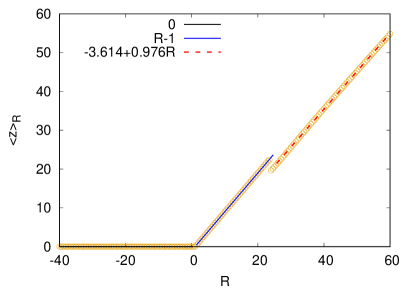
Figure 8: (Color online) $\langle z\rangle_{R}$ vs $R$ numerically computed in the standard Lorenz system (symbols). Notice that the curve is well approximated, in the range of interest, by the piecewise linear function in Eqs. (17), see legend.

In order to model $\langle xy\rangle_{\bm{X}}$, we first impose stationarity i.e. $\langle\dot{\bm{x}}\rangle_{\bm{X}}=0$ which, applied to the third line of Eqs. (10), yields

$$\langle xy\rangle_{\bm{X}}=b\langle z\rangle_{\bm{X}}\,.$$ (15)

Inserting the result (15) in the equation for $Y$ in Eqs. (6) we obtain $\dot{Y}=R_{s}X-ZX-Y-\epsilon_{s}\,b\,\langle z\rangle_{\bm{X}}$. Now we need to determine $\langle z\rangle_{\bm{X}}$. For this purpose, we notice that the equation for $\dot{y}$ in Eqs. (10) can be rewritten as

$$\dot{y}=c[Rx-zx-y]\qquad\mathrm{with}\qquad R=R_{f}+\frac{\epsilon_{f}}{c}Y\,.$$ (16)

Exploiting the adiabatic principle we assume $Y$ (the slow variable) as fixed so that Eqs. (10) with the second equation substituted with Eq. (16) become the standard Lorenz model, a part from an inessential change of time scale. Thus, we can now evolve the standard Lorenz model and compute $\langle z\rangle_{R}$ (where _R is just to remind the $R$ dependence that will be reflected in a $Y$ dependence via Eq. (16)), which is shown in Fig. 8. As one can see $\langle z\rangle_{R}$ depends on $R$ approximately as follows:

$$\langle z\rangle_{R}\approx\left\{\begin{array}[]{ll}0&R<1\\ R-1&1\leq R\lesssim 24.74\\ 0.976R-3.614&R\gtrsim 24.74\end{array}\right.$$ (17)

We remind that $R_{c}=24.74$ is the critical value at which the fixed point

$$z^{*}=(R-1)\Theta(R-1)\,,$$ (18)

(where $\Theta$ is the Heaviside step function) loses its stability. Remarkably, $\langle z\rangle_{R}$ remain close to $z^{*}$ also for $R>R_{c}$. The second expression in Eqs. (17), or equivalently Eq. (18), yields

$$\langle xy\rangle_{Y}=b(R_{f}-1+(\epsilon_{f}/c)Y)\Theta(R_{f}-1+(\epsilon_{f}/c)Y)\,.$$ (19)

Using the numerical values of the constants ($b=8/3$, $R_{f}=45$ and $\epsilon_{f}=10$), the above expression provides the estimate $\langle xy\rangle_{Y}\approx(117.33+26.67\,Y/c)\,\Theta(117.33+26.67Y/c)$ while using the third expression of Eqs. (17) yields model (11) that we used to compare with the network, i.e.

$$\langle xy\rangle_{Y}\!=\!(107.5\!+\!26.04Y/c)\,\Theta((107.5\!+\!26.04Y/c)\,.$$ (20)

For $c=10$, the latter expression is very close to the (numerically obtained) conditional average $\langle xy|Y\rangle$(Fig. 9a), confirming that the scale separation is wide enough for the adiabatic approximation to work almost perfectly. We notice that for $c=10$ the typical range of variation of $Y$ is such that $R$ mostly lies in the region of the third branch of Eqs. (17), explaining the validity of the approximation.

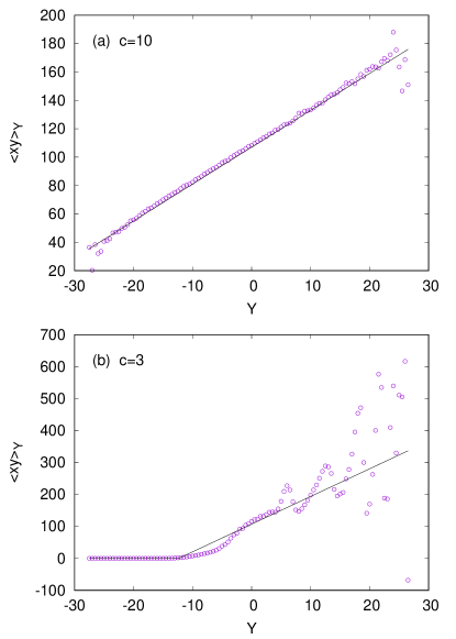
Figure 9: (Color online) Numerically computed conditional averages (symbols) $\langle xy|Y\rangle$ for (a) $c=10$ and (b) $c=3$ and the corresponding multiscale (adiabatic) averages $\langle xy\rangle_{Y}$ given by Eqs. (20) (solid curve). For $c=10$ the two curves overlap.

Conversely, for the case $c=3$, as shown in Fig. 9b the approximation is much cruder and important deviations are present especially for large positive values of $Y$. Indeed, in general,

$$\langle xy\rangle_{\bm{X}}\neq\langle xy|\bm{X}\rangle$$

i.e. multiscale average obtained via the adiabatic principle and the conditional average are not equivalent since, in general, $\langle\dot{\bm{x}}|\bm{X}\rangle\neq 0$. In this case the values of all slow variables will matter in building a proper effective model, a hard task even for the simple Lorenz model here considered. However, as shown in Fig. 3, even in this case the reservoir computing approach is quite performing even though it is not straightforward to decipher the model it was able to devise.

Appendix C Discussion on various hybrid schemes implementations

The hybrid scheme discussed in Sec. II.3 allows for highlighting the properties of the reservoir, but it is just one among the possible choices. Here, we briefly discuss three general schemes.

Let us assume, for simplicity, that our dynamical system, with state variables $\bm{s}=(s_{1},...,s_{n})$, is described by the equation $\bm{s}(t+1)=\bm{f}(\bm{s}(t))$, which is unknown. Here, without loss of generality, we use discrete time dynamics and that we want to forecast the whole set of state variables, this is just for the sake of simplicity of the presentation. Provided we have an imperfect model, $\bm{s}(t+1)\approx\bm{f}_{m}(\bm{s}(t))$, for its evolution, we have basically three options for building a hybrid scheme.

A first possibility is to approximate via machine learning only the part of the signal that is not captured by the model $\bm{f}_{m}(\bm{s}(t))$. In other terms, one writes a forecast as

$$\hat{\bm{s}}(t+1)=\bm{f}_{m}(\bm{s}(t))+\bm{\delta}_{n}(\bm{s}(t))$$ (21)

where the residual $\bm{\delta}_{n}$ is given by the network, and can be learned from a set of input-output pairs $\{\bm{s}(t),\bm{s}(t+1)-\bm{f}_{m}(s(t))\}_{t=-T}^{0}$ according to some supervised learning algorithm. In our framework, the hybrid network should be trained with the usual input but with target output given by the difference between the true value of $\bm{s}(t+1)$ and the model forecast $\bm{f}_{m}(\bm{s}(t))$.

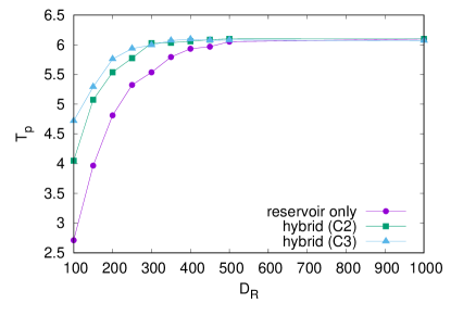
Figure 10: (Color online) Average (over $10^{4}$ initial conditions) predictability times are shown for reservoir only and two hybrid implementations ($\Delta t=0.1$ and $c=10$). The green line corresponds to the hybrid scheme (22), blue lines to the hybrid scheme (23) and purple lines to the reservoir only baseline.

A second possibility is to add the available model prediction $\bm{f}_{m}(\bm{s}(t))$ to the input $\bm{s}(t)$, obtaining an augmented input $(\bm{s}(t),\bm{f}_{m}(\bm{s}(t))$ for the network. In this case, the forecast reads as

$$\hat{\bm{s}}(t+1)=\bm{f}_{n}(\bm{s}(t),\bm{f}_{m}(\bm{s}(t)).$$ (22)

Clearly, if the model based prediction is very accurate, the network will try to approximate the identity function. The network should be trained with a set of input-outputs pairs $\{(s(t),f_{m}(s(t))),s(t+1)\}_{t=-T}^{0}$. This is the approach we have implemented in this article, in order to evaluate the performance of the reservoir.

A third possibility is to combine the two previous options, which is the approach followed in Ref. [15]. In this case, the forecast is obtained as:

$$\hat{\bm{s}}(t+1)=\mathbb{A}\,\bm{f}_{m}(\bm{s}(t))+\mathbb{B}\,\bm{\delta}_{n}(\bm{s}(t),\bm{f}_{m}(s(t))\,,$$ (23)

where the matrices $\mathbb{A}$ and $\mathbb{B}$ should be optimized, along with $\delta_{n}$. This last option is a special case of the second scheme, describing a residual multilayered neural network with a linear output layer.

For the sake of completeness, in Fig. 10 we show how this last architectures compares with the one we used in Figs. 5 and 6 in terms of predictability. It consists in taking the optimized linear combination of the predictions from the hybrid net and the imperfect model. Namely, one augment the $r^{*}$ array as $\tilde{\bm{r}}^{*}=(\bm{r}^{*},\bm{f}_{m})$ and then optimizes $\mathbb{W}_{O}$ to achieve $\bm{v}(t+1)=\hat{\bm{s}}(t+1)\approx\mathbb{W}_{O}\tilde{\bm{r}}^{*}(t)$. As one can see, the main effect is to slightly shift the predictability-vs-size curve leftward, meaning that optimal performance can be achieved with a slightly smaller network. However, the improvement quickly disappears when the reservoir size increases.

References

- Argall et al. [2009] B. D. Argall, S. Chernova, M. Veloso, and B. Browning, Robot. Auton. Sys. 57, 469 (2009).
- Libbrecht and Noble [2015] M. W. Libbrecht and W. S. Noble, Nature Rev. Genet. 16, 321 (2015).
- He et al. [2019] J. He, S. L. Baxter, J. Xu, J. Xu, X. Zhou, and K. Zhang, Nature Med. 25, 30 (2019).
- Carleo et al. [2019] G. Carleo, I. Cirac, K. Cranmer, L. Daudet, M. Schuld, N. Tishby, L. Vogt-Maranto, and L. Zdeborová, Rev. Mod. Phys. 91, 045002 (2019).
- Verstraeten et al. [2007] D. Verstraeten, B. Schrauwen, M. d’Haene, and D. Stroobandt, Neural Net. 20, 391 (2007).
- Schrauwen et al. [2007] B. Schrauwen, D. Verstraeten, and J. Van Campenhout, in Proc. 15th Europ. Symp. Artif. Neural Netw. (2007) pp. 471–482.
- Jaeger [2001] H. Jaeger, German Nat. Res. Center Infor. Tech. GMD Technical Report 148, 13 (2001).
- Lukoševičius and Jaeger [2009] M. Lukoševičius and H. Jaeger, Comp. Sci. Rev. 3, 127 (2009).
- Jaeger and Haas [2004] H. Jaeger and H. Haas, Science 304, 78 (2004).
- Pathak et al. [2017] J. Pathak, Z. Lu, B. R. Hunt, M. Girvan, and E. Ott, Chaos 27, 121102 (2017).
- Pathak et al. [2018a] J. Pathak, B. Hunt, M. Girvan, Z. Lu, and E. Ott, Phys. Rev. Lett. 120, 024102 (2018a).
- Lu et al. [2018] Z. Lu, B. R. Hunt, and E. Ott, Chaos 28, 061104 (2018).
- Vlachas et al. [2018] P. R. Vlachas, W. Byeon, Z. Y. Wan, T. P. Sapsis, and P. Koumoutsakos, Proc. Royal Soc. A 474, 20170844 (2018).
- Nakai and Saiki [2018] K. Nakai and Y. Saiki, Phys. Rev. E 98, 023111 (2018).
- Pathak et al. [2018b] J. Pathak, A. Wikner, R. Fussell, S. Chandra, B. R. Hunt, M. Girvan, and E. Ott, Chaos 28, 041101 (2018b).
- Wikner et al. [2020] A. Wikner, J. Pathak, B. Hunt, M. Girvan, T. Arcomano, I. Szunyogh, A. Pomerance, and E. Ott, Chaos 30, 053111 (2020).
- Warhaft [2002] Z. Warhaft, Proc. Nat. Acad. Sci. 99, 2481 (2002).
- Peixoto and Oort [1992] J. P. Peixoto and A. H. Oort, Physics of climate (New York, NY (United States); American Institute of Physics, 1992).
- Pedlosky [2013] J. Pedlosky, Geophysical fluid dynamics (Springer, 2013).
- Lorenz [1995] E. N. Lorenz, in ECMWF Seminar Proceedings on Predictability, Vol. 1 (ECMWF, Reading, UK, 1995).
- Aurell et al. [1996] E. Aurell, G. Boffetta, A. Crisanti, G. Paladin, and A. Vulpiani, Phys. Rev. Lett. 77, 1262 (1996).
- Cencini and Vulpiani [2013] M. Cencini and A. Vulpiani, J. Phys. A 46, 254019 (2013).
- Boffetta et al. [2000] G. Boffetta, A. Celani, M. Cencini, G. Lacorata, and A. Vulpiani, J. Phys. A 33, 1313 (2000).
- Sanders et al. [2007] J. A. Sanders, F. Verhulst, and J. Murdock, Averaging methods in nonlinear dynamical systems, Vol. 59 (Springer, 2007).
- Pavliotis and Stuart [2008] G. Pavliotis and A. Stuart, Multiscale methods: averaging and homogenization (Springer, 2008).
- Werbos [1990] P. J. Werbos, Proc. IEEE 78, 1550 (1990).
- Larger et al. [2017] L. Larger, A. Baylón-Fuentes, R. Martinenghi, V. S. Udaltsov, Y. K. Chembo, and M. Jacquot, Physical Review X 7, 011015 (2017).
- Tanaka et al. [2019] G. Tanaka, T. Yamane, J. B. Héroux, R. Nakane, N. Kanazawa, S. Takeda, H. Numata, D. Nakano, and A. Hirose, Neural Net. 115, 100 (2019).
- Pikovsky et al. [2003] A. Pikovsky, J. Kurths, and M. Rosenblum, Synchronization: a universal concept in nonlinear sciences, Vol. 12 (Cambridge university press, 2003).
- Rivkind and Barak [2017] A. Rivkind and O. Barak, Phys. Rev. Lett. 118, 258101 (2017).
- Jiang and Lai [2019] J. Jiang and Y.-C. Lai, Phys. Rev. Res. 1, 033056 (2019).
- Note [1] In [10, 12] it is suggested that this choice respects the symmetries of the Lorenz system. In general, any reasonably nonlinear function of should suffice [7].
- Milano and Koumoutsakos [2002] M. Milano and P. Koumoutsakos, J. Comput. Phys. 182, 1 (2002).
- Wan et al. [2018] Z. Y. Wan, P. Vlachas, P. Koumoutsakos, and T. Sapsis, PloS one 13, e0197704 (2018).
- Weymouth and Yue [2013] G. D. Weymouth and D. K. P. Yue, J. Ship Res. 57, 1 (2013).
- Boffetta et al. [1998] G. Boffetta, P. Giuliani, G. Paladin, and A. Vulpiani, J. Atmos. Sci. 55, 3409 (1998).
- Carlu et al. [2019] M. Carlu, F. Ginelli, V. Lucarini, and A. Politi, Nonlin. Proc. Geophys. 26, 73 (2019).
- Carmichael et al. [2019] Z. Carmichael, H. Syed, and D. Kudithipudi, in Proc. 7th Annual Neuro-inspired Comput. Elements Workshop (2019) pp. 1–10.
- Lu et al. [2017] Z. Lu, J. Pathak, B. Hunt, M. Girvan, R. Brockett, and E. Ott, Chaos 27, 041102 (2017).
- Meneveau and Katz [2000] C. Meneveau and J. Katz, Annu. Rev. Fluid Mech. 32, 1 (2000).
- Sagaut [2006] P. Sagaut, Large eddy simulation for incompressible flows: an introduction (Springer, 2006).
- Biferale et al. [2017] L. Biferale, A. A. Mailybaev, and G. Parisi, Phys. Rev. E 95, 043108 (2017).
- Note [2] Notice that if at least one eigenvalue is zero.
- Kennedy and Eberhart [1995] J. Kennedy and R. Eberhart, in Proceedings of ICNN’95-International Conference on Neural Networks, Vol. 4 (IEEE, 1995) pp. 1942–1948.