A method to suppress local minima for symmetrical DOPO networks

Abstract

Coherent Ising machine (CIM) implemented by degenerate optical parametric oscillator (DOPO) networks can solve some combinatorial optimization problems. However, when the network structure has a certain type of symmetry, optimal solutions are not always detected since the search process may be trapped by local minima. In addition, a uniform pump rate for DOPOs in the conventional operation cannot overcome this problem. In this paper proposes a method to avoid trapping of the local minima by applying a control input in a pump rate of an appropriate node. This controller breaks the symmetrical property and causes to change the bifurcation structure temporarily, then it guides transient responses into the global minima. We show several numerical simulation results.

1 Introduction

In recent years, the combinatorial optimization problems appears in various fields.

There are a lot of algorithms to tackle them, but many Non-deterministic polynomial hard (NP-hard) problems require exponentially increasing computation time as the problem becomes larger.

The Ising model is a mathematical formulation mimicking the ferromagnetism dynamics, and the searching problem of its ground state (namely the Ising problem[1]) can encode MAX-CUT problem[2, 3] for 3D network graphs. The solution obtained from the coherent Ising machine (CIM) takes a good value as an approximate solution of the Ising problem. It has been demonstrated that Ising problems is solved by DOPO networks which is one of the implementations of CIM[4]. In the network, each DOPO corresponds to the Ising spin in the problem, and the network state is obtained as a solution when the pump rate exceeds the oscillation threshold.

Wang, et al. [5] provided theoretical background of the DOPO and showed the performance theoretical and numerically, i.e., the coupled DOPOs can seek the optimal solution as a ground state of the Ising model. In most cases, the DOPO network gets the ground state by gradually pumping all oscillators. However, the solution of the DOPO network is not always optimal[6]. In the case of gradually pumping DOPOs, local minima, which are not the ground state, appear earlier than the optimal solution, therefore they disturb finding the ground state[7, 8]. As a result, the performance of the CIM decreases.

Ito investigated bifurcation problems in a network configured by eight DOPOs[9]. By choosing a pump rate of a specific node and a unified pump rates of other nodes as a pair of parameters, several bifurcation diagrams composed by super-critical and sub-critical pitchfork bifurcations and tangent bifurcations have been obtained. The analysis of their structures reveals that the variation of the unified pump rate tends to be confined into a valley sectioned by bifurcation curves. Inside of the valley, the optimal solutions are concealed by other local minima. This situation is caused by pitchfork bifurcations due to a symmetrical property, thus we guess that the performance of the CIM may be improved by breaking a symmetric property on purpose. In this paper, we propose a method to suppress local minima by adjusting not the unified pump rate but the specific one. This control perturbs the symmetrical property of the DOPO network temporarily and guides the trajectory into the global solution. We show simulation results for several kinds of symmetric DOPO networks.

2 DOPO networks

A DOPO system is described by the following $c$-number Langevin equations[4, 5]:

$$\begin{array}[]{rll}\displaystyle\frac{dc_{j}}{dt}&=&\displaystyle(p-1+(c^{2}_{j}-s^{2}_{j}))c_{j}+\sum_{l=1,l\not=j}^{N}\xi_{jl}c_{l},\\ \displaystyle\frac{ds_{j}}{dt}&=&\displaystyle(p-1-(c^{2}_{j}-s^{2}_{j}))s_{j}+\sum_{l=1,l\not=j}^{N}\xi_{jl}s_{l},\\ &&j=1,2,\ldots,N\end{array}$$ (1)

where $c$ and $s$ are the normalized in-phase and quadrature-phase components, respectively. $p$ is the pump rate, $\xi$ is the coupling coefficient of DOPO network. A detailed description of the quantum models is shown in Refs.[10, 11]. In the numerical simulations of Eq. (1), we experimentally observe that $s$ tend to be vanished as time goes on. Thus the system can be simplified as follows:

$$\frac{dc_{j}}{dt}=(p-1)c_{j}-c^{3}_{j}+\sum_{l=1,l\not=j}^{N}\xi_{jl}c_{l}.$$ (2)

If we define the state vector $\bm{c}$ and edge weight matrix $\Xi$ as:

$$\bm{c}=\left(\begin{array}[]{c}c_{1}\\ c_{2}\\ \vdots\\ c_{N}\end{array}\right),~{}~{}\Xi=\left(\begin{array}[]{cccc}0&\xi_{12}&\ldots&\xi_{1N}\\ \xi_{21}&0&&\xi_{2N}\\ \vdots&&\ddots&\\ \xi_{N1}&\xi_{2N}&&0\end{array}\right),$$ (11)

where, $\xi_{jl}$ is a coupling coefficient between nodes j and l. If node $i$ and $j$ is coupled, $\xi_{ij}=\xi_{ji}=\xi$, but if not, $\xi_{ij}=\xi_{ji}=0$. Then Eq. 1 can be derived as Eq. (12).

$$\frac{d\bm{c}}{dt}=\bm{f}(\bm{c})+\Xi\bm{c},$$ (12)

where $\bm{f}(\bm{c})=(f(c_{1}),f(c_{2}),\ldots,f(c_{N}))^{T}$. In Eq. (2), the Jacobian matrix is derived as:

$$J(\bm{c})=\frac{\partial\bm{f}}{\partial\bm{c}}+\frac{1}{\xi}\Xi.$$ (13)

MAX-CUT problem is a problem that divides nodes of a graph into two groups and maximizes the number of edges cut. The Ising Hamiltonian can be applied to the number of cuts in the MAX-CUT problem[3]. The number of cuts when describing the MAX-CUT problem in CIM using DOPO networks is defined as:

$$\mathop{\rm cut}(\Xi,\chi)=-\sum_{j=1}^{N}\sum_{l=1,l\not=j}^{N}J_{jl}\chi_{j}\chi_{l},$$ (14)

where, $\chi_{j}={c_{j}}/{|c_{j}|}$., $J_{jl}$ is the generic element of the coupling matrix which defined as $J_{jl}=0$ if $\xi_{jl}=0$ , otherwise $J_{jl}=1$. The relaxation function in Eq. (15) is the smallest value when the DOPO network is in the optimal solution.

$$\eta(\bm{c})=\sum_{j=1}^{N}(p-c_{j}^{2}-1)=-\sum_{j=1}^{N}\sum_{l=1,l\neq j}^{N}\xi_{jl}\frac{c_{l}}{c_{j}}.$$ (15)

Figure 1 gives MAX-CUT problems and their optimal solutions treated in this paper. The cut is determined by the sign of the solution $\bm{c}$ in Eq. (2), e.g., $c_{1},c_{2},c_{7},c_{8}$ take positive value and $c_{3},c_{4},c_{5},c_{6}$ take negative value at Fig. (1)(a). Note that both graphs contain certain classes of symmetry and pitchfork bifurcations are the major bifurcation phenomena of the DOPO networks[12].

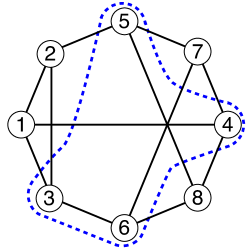
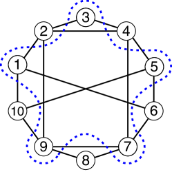
(a) $N=8$	(b) $N=10$

Figure 1: MAX-CUT problems and one of their optimal solutions. The number of edges which the dashed line intersects give the maximum for each graph.

3 Pump rate and its control

We may obtain candidates of solutions of the problem as equilibrium points of Eq. (1). From appropriate initial values, the solution may fall into one of stable equilibrium points according to both global solutions and local minima after a transition state. To compute equilibrium points, we apply Newton’s method by letting the left-hand of Eq. (2) be zero, with providing initial points by a brute-force strategy with Mersenne twista[13]. Figure 2(a) and (b) are stable equilibria of Eq. (2) corresponding to Fig. 1 (a) and (b), respectively. There are many unstable equilibria from the pitch-fork bifurcation around these attractors, but we do not visualize them. Red and blue points are local minima and optimal solutions, respectively. The pump rate is $p=0.92$ both of them.

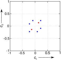
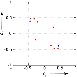
(a)	(b)

Figure 2: Stable equilibria. Blue points are the optimal solutions. (a): corresponding to Fig. 1(a), (b): corresponding to Fig. 1(b). Both are obtained with $p=0.92$.

The performance of the machine is improved by gradually increasing $p$ from zero to one [14] compared with the fixed pump rate. That is, in the hardware implementation, we practically increase the pump rate from a low value, and gradually increase it near one monotonically.

3.1 Bifurcations of equilibria with pump rates

Figure 3 shows the one-parameter bifurcation diagram for the case $N=8$ corresponding to Fig. 1(a) and this incremental pump rate process tracks this diagram from left to right. At any value of $p$, several random initial values are scattered to find the equilibrium point.

Gray points show the origin stable point corresponding to no cut. As $p$ increases, the system receives a pitch-fork bifurcation. Therefore, two symmetrical equilibrium points occur near the origin. In this case, they are corresponding to local minima. If $p$ increases further, and at $p=0.909$, the system causes a multiple tangent bifurcation, and new four equilibria appear. Indeed, they are optimal solutions (blue). Since local minima and optimal solutions coexist in $0.909<p<1$. There is no parameter set at which only the optimal solution occurs. With this incremental pump rate process, local minima as sub-optimal solution is detected at first, and the state is trapped to the same solution against further increment of the pump rate. It causes the performance deterioration of the machine.

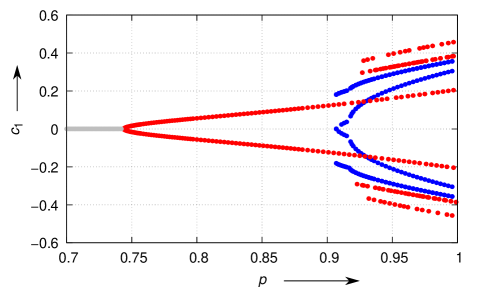
Figure 3: One-parameter bifurcation diagram ($N=8$).

Let $p_{j}$ be an individual pump rate according to the node $j$ and assume it is adjustable. Also assume that and other pump rates are fixed. Figure 4 shows an incremental process of $p_{4}$ for Fig. 1(a). The vertical axis shows the amplitude of $c_{1}$. We increase $p_{4}$ from 0.9 to 1 gradually. Blue and red point show optimal solutions and local minima, respectively. The red solution meets a tangent bifurcation ($G$) near 0.99, and then it disappears. Thus, there is parameter sets $0.99<p_{4}$ that gives only optimal solutions by adjusting the pump rate individually.

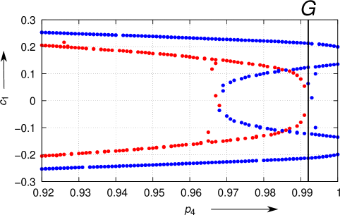
Figure 4: $c_{1}$-$p_{4}$ bifurcation diagram ($N=8$).

Now we investigate a relationship between optimal solutions and the pump rate. As mentioned above, not only global minima but also local minima are generated by pitchfork bifurcations induced from the symmetrical configuration of the network. If the system is trapped into local minima, the value of the relaxation Eq. (15) becomes high since this stable situation is given by the forcing energy frustration to a part of nodes[6]. While, the precede work[9] suggested that a possibility of the control method to avoid trapping to local minima by adjusting pump rates of some DOPOs. This suppresses some bifurcation phenomena by breaking the symmetry of the dynamical system on purpose. It can be called as a “bifurcation avoidance control” so to speak. Figure 5 shows the $p$-$p_{j}$ bifurcation diagram at $N=8$, where $G$ and $pf$ shows the tangent bifurcation and pitchfork bifurcation, respectively. We pick up a pump rate $p_{j}$ for one of DOPOs, and suppose a uniform pump rate $p$ for other DOPOs. Only local minima occur in (i), both local minima and the optimal solutions are mixed in (ii), and only optimal solutions occur in (iii).

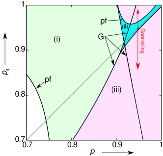
Figure 5: $p$-$p_{j}$ bifurcation diagram.

On the gray diagonal line in Fig. 5, the pump rate set does not reach (iii). However, controlling $p_{4}$ independently, as indicated by the red arrow, the pump rate set reaches (iii).

3.2 Pump rate control scheme

In the Sect. 3.1, we recognize that there is the pump rate set in which only the optimal solution can be obtained by setting the pump rate $p_{j}$ independently. Although, with the method, it is necessary to specify the amount to raise the pump rate in advance. The pump rate set which is only the optimal solution can be obtained from the relation with $p_{j}$ and $c_{j}$. The frustration at a local minima imposed on nodes with small $|c_{j}|$. To increase the $|c_{j}|$, increase the pump rate $p_{j}$ of a node with the smallest $|c_{j}|$. Therefore, consider a function that automatically adjusts $p_{j}$ according to the size of $|c_{j}|$, and replace $p_{j}$ with the pump rate of the node whose absolute value is small. Assume that a variable range of the pump rate is from zero to one, then $e^{-|c_{j}|}$ can be adopted as a reasonable adjustment control value. As a result, the pump rate $p_{j}$ can be regarded as a function depending on the state variable, and the parameter can be set automatically.

We propose a dynamic pump rate $p_{j}$ described as follows:

$$p_{j}=\beta e^{-|c_{j}|},$$ (16)

where, $\beta$ is gain of control. In this paper we set $\beta=1$. When $c_{j}$ takes a smaller value, $p_{j}$ inflates. Figure 6 is the change of $p_{j}$. In the case of Fig. 5, $p_{4}$ is controlled since $|c_{4}|$ is the smallest. $p_{4}$ rises according to the exponential function of Fig. 6. As a result, the pump rate set moves to (iii).

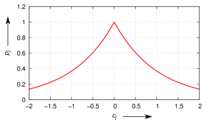
Figure 6: The example graph of Eq. (16), where $\beta=1$.

Figure 7 depicts the procedure of the control. When the calculation starts and the system becomes stable near the equilibrium point, find the index $j$ of the node with the smallest $|c_{j}|$. Then, replace the pump rate of the $j$-th node with $e^{-|c_{j}|}$. The number of replacing pump rate is not specified in particular, excessive control causes the performance degradation, so it is necessary to add control while monitoring the value of the relaxation function. In the following trials, we apply this procedure once.

Figure 7: The flowchart of the control.

4 Simulation results

Figure 8 shows the controlling result for $N=8$ DOPO networks shown in Fig. 1(a) with the coupling coefficient $\xi=-0.1$. We fix the unified pump rate as $p=0.92$. As far as we checked, $|c_{j}|$ for all equilibrium points is less than unity, thus we put $\beta=1$. The system runs without the controlling until $t=400$, then it converges the local minima, and has distribution of $c_{1-8}$ with large deviation. In the case of the trial in Fig. 8, the node with $j=4$ is the smallest $|c_{j}|$, so $p_{4}$ is selected as the control target. The controlling starts after that, and the pump rate $p_{4}$ is derived from Eq. (16). It is confirmed that the sign inversion of $c_{1}$ occurs after $t=400$, and the number of cuts is improved from $12$ to $16$ by this sign inversion. A red arrow in Fig. 5 represents the change of $p_{4}$ in the parameter plane. Note that, the local minima exist in the (i) region, the optimal and local minima coexist in the (ii) region. In the (iii) region, the DOPO has only optimal solutions. The parameter set moves from the blue region to the red region by the proposed controller through the tangent bifurcation. As a result, our controller can avoid the local minima. By 100 trials with random initial values, our controller improve the probability of finding the optimal solution from $84\%$ to $100\%$.

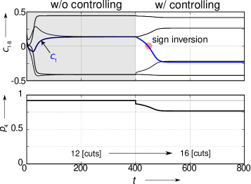
Figure 8: Control response for the $N=8$ network. The controller adjusts the pump rate $p_{4}$.

The control response for the $N=10$ DOPO network is shown as Fig. 9. Here, the network structure is shown in Fig. 1(b), where the coupling coefficient $\xi=-0.1$ and the common pump rate is $p=0.92$. We choose the adjustable pump rate as $p_{2}$. Similar to Fig. 8, the control improves the number of cuts from $18$ to $26$.

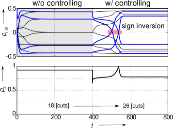
Figure 9: Control response for the $N=10$ network. The controller adjusts the pump rate $p_{2}$.

Figure 10 shows the relationship between eight nodes on a steady-state with/without the proposed controller corresponding to the simulation results in Fig. 8. Note that, the size of each node is scaled by the absolute values of $c_{j}$ of the node $j$. When the network converges to local minima solutions without controlling, the difference between maxima and minima circles becomes large; therefore node five and eight indirectly frustrate node one. Thus, they have $|c_{j}|$ values larger than other nodes. However, the difference in the size of the nodes is relieved because the network converges to the global optimal solution from the local minima by the proposed controller.

Furthermore, Fig. 12 shows the transition of the relaxation function in each graph. The change of the node size in the graph of Fig. 10 is evaluated by Fig. 12(a). The $\eta(\bm{c})$ of Fig. 10 decreases at $t=400$ due to the addition of control. Fig. 12(c) and (d) are $N=16$ and $N=20$ nodes graph which are Fig. 11. Similar to Fig. 1(a) and (b), Fig. 11 also have symmetry. Initial pump rate of $N=16$ and $N=20$ are $p=0.98$. It is found that the relaxation function decreased after control in all graphs, and the number of cuts also increased. The number of cuts for $N=16$ and $N=20$ improves from $28$ to $32$ and $36$ to $40$, respectively.

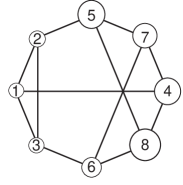
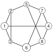
(a)	(b)

Figure 10: (a): before controlling, (b): after controlling.

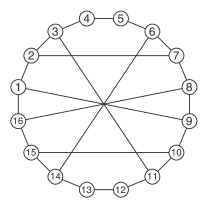
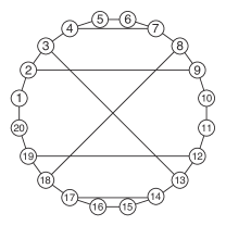
(a) $N=16$	(b) $N=20$

Figure 11: The graph of $N=16$ and $N=20$.

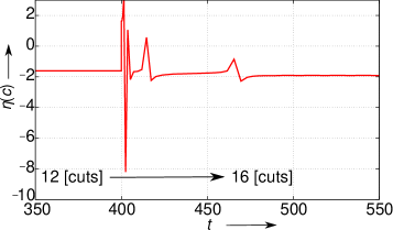
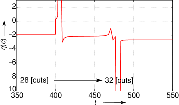
(a)	(b)
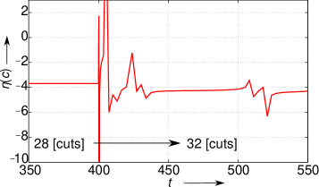
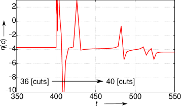
(c)	(d)

Figure 12: $\scriptstyle\mbox{Transitions of the relaxation function.}\atop\scriptstyle\mbox{ (a): $N=8$, (b): $N=10$, (c): $N=16$, (d): $N=20$.}$

Table 1 summarizes the probability of the optimal state with and without the proposed controller. For the four networks, the proposed controller can suppress the local minima, and can improve the probability of the optimal solutions.

Table 1: Probability of the optimal solution for w/o and w/ proposed controller. The number of trials is 100. The initial state is given by random values.

number of nodes	w/o control	w/ control
$8$	84%	100%
$10$	78%	100%
$16$	92%	97%
$20$	88%	100%

5 Conclusion

We propose a method to avoid local minima for symmetrical DOPO networks. We design new controlling scheme for the improvement of the DOPO network as the MAX-CUT solver. We summarize the proposal method and the results to following items.

1. Conventionally, the pump rate was set uniformly, although we recognize that the local minima disappeared due to tangent bifurcation when the pump rate was set individually at each node.

2. There is a pump rate set that can obtain only the optimal solution in the $p_{j}$-$p$ bifurcation diagram of the DOPO network.

3. From the bifurcation diagram and the structure in the DOPO network, we proposed a controlling method that automatically sets the pump rate by the exponential function.

4. Our controller improves the probability of success for optimal solution search in the four symmetrical DOPO networks.

Next, the future tasks are follows:.

1. In this paper, the relaxation function was monitored for the number of replacing pump rate, although we need to find out how to determine the most effective number of replacing.

2. We try to systematic explanations of the performance of proposed controller based on the bifurcation theory, however since there is a non-differentiable absolute value function in the control term, the bifurcation analysis becomes difficult. This problem can be avoided by replacing $e^{-|c_{j}|}$ with a quadratic function such as $1-{c_{j}}^{2}$, but the performance comparison between two control terms is required.

This paper is under article submission and will be published on Nonlinear Theory and Its Applications, IEICE(Vol.E11-N, No.4, Oct. 2020). All authors agree to post this preprint to arXiv.

References

- [1] E. Ising, “Beitrag zur theorie des ferromagnetismus,” Zeitschrift für Physik, vol. 31, no. 1, pp. 253–258, 1925.
- [2] R. M. Karp, “Reducibility among combinatorial problems,” in Complexity of Computer Computations, pp. 85–103, Boston, MA: Springer US, 1972.
- [3] A. Galluccio, M. Loebl, and J. Vondrák, “New algorithm for the Ising problem: Partition function for finite lattice graphs,” Physical Review Letter, vol. 84, no. 26, pp. 5924–5927, 2000.
- [4] Z. Wang, A. Marandi, K. Wen, R. L. Byer, and Y. Yamamoto, “Coherent Ising machine based on degenerate optical parametric oscillators,” Physical Review A, vol. 88, no. 6, p. 063853 (9 pages), 2013.
- [5] Z. Wang, Coherent computation in Degenerate Optical Parametric Oscillators. PhD thesis, Stanford University, Stanford University, Stanford, CA 94305 USA, 2015.
- [6] Y. Haribara, S. Utsunomiya, and Y. Yamamoto, “A coherent Ising machine for MAX-CUT problems: Performance evaluation against semidefinite programming and simulated annealing,” in Principles and Methods of Quantum Information Technologies, vol. 911 of Lecture Notes in Physics, ch. 12, pp. 251–262, Springer, Japan, 2016.
- [7] K. Takata, S. Utsunomiya, and Y. Yamamoto, “Transient time of an Ising machine based on injection-locked laser network,” New Journal of Physics, vol. 14, p. 013052, 2012.
- [8] K. Takata, A. Marandi, R. Hamerly, Y. Haribara, D. Maruo, S. Tamate, H. Sakaguchi, S. Utsunomiya, and Y. Yamamoto, “A 16-bit coherent Ising machine for one-dimensional ring and cubic graph problems,” Scientific Reports, vol. 6, p. 34089, 2016.
- [9] D. Ito, T. Ueta, and K. Aihara, “Bifurcation analysis of eight coupled degenerate optical parametric oscillators,” Physica D: Nonlinear Phenomena, vol. 372, pp. 22–30, 2018.
- [10] T. Shoji, K. Aihara, and Y. Yamamoto, “Quantum model for coherent Ising machines: Stochastic differential equations with replicator dynamics,” Phys. Rev. A, vol. 96, no. 5, p. 053833, 2017.
- [11] A. Yamamura, K. Aihara, and Y. Yamamoto, “Quantum model for coherent Ising machines: Discrete-time measurement feedback formulation,” Phys. Rev. A, vol. 96, no. 5, p. 053834, 2017.
- [12] T. Ueta, H. Miyazaki, T. Kousaka, and H. Kawakami, “Bifurcation and chaos in coupled BVP oscillators,” International Journal of Bifurcation and Chaos, vol. 14, no. 04, pp. 1305–1324, 2004.
- [13] M. Matsumoto and T. Nishimura, “Mersenne twister: A 623-dimensionally equidistributed uniform pseudo-random number generator,” ACM Transactions on Modeling and Computer Simulation, vol. 8, no. 1, pp. 3–30, 1998.
- [14] K. Takata and Y. Yamamoto, “Data search by a coherent Ising machine based on an injection-locked laser network with gradual pumping or coupling,” Physical Review A, vol. 89, p. 032319, 2014.