The Monte Carlo Transformer: a stochastic self-attention model for sequence prediction

Abstract

This paper introduces the Sequential Monte Carlo Transformer, an original approach that naturally captures the observations distribution in a transformer architecture. The keys, queries, values and attention vectors of the network are considered as the unobserved stochastic states of its hidden structure. This generative model is such that at each time step the received observation is a random function of its past states in a given attention window. In this general state-space setting, we use Sequential Monte Carlo methods to approximate the posterior distributions of the states given the observations, and to estimate the gradient of the log-likelihood. We hence propose a generative model giving a predictive distribution, instead of a single-point estimate.

1 Introduction

Many critical applications (e.g. medical diagnosis or autonomous driving) require accurate forecasts while detecting unreliable predictions, that may arise from anomalies, missing information, or unknown situations. While neural networks excel at predictive tasks, they often solely output a single-point estimate, lacking uncertainty measures to assess their confidence about their predictions. To overcome this limitation, an open research question is the design of neural generative models able to output a predictive distribution instead of single point-estimates. First, such distributions would naturally provide the desired uncertainty measures over the model predictions. Secondly, learning algorithms can build upon such uncertainty measurements to improve their predictive performance such as active learning [Campbell et al., 2000] or exploration in reinforcement learning [Geist and Pietquin, 2010, Fortunato et al., 2018]. Thirdly, they may better model incoming sources of variability, such as observation noise, missing information, or model misspecification.

On the one hand, Bayesian statistics offer a mathematically grounded framework to reason about uncertainty, and has long been extended to neural networks [Neal, 2012, MacKay, 1992]. Among recent methods, Bayesian neural networks (BNNs) estimate a posterior distribution of the target given the input variables by injecting stochasticity in the network parameters [Blundell et al., 2015, Chung et al., 2015] or casting dropout as a variational predictive distribution  [Gal and Ghahramani, 2015]. However, such models tend to be overconfident, leading to poorly calibrated uncertainty estimates [Foong et al., 2019]. On the other hand, concurrent frequentist approaches have been developed to overcome the computational burden of BNNs, by either computing ensembling networks [Huang et al., 2017, Igl et al., 2018] or directly optimizing uncertainty metrics [Pearce et al., 2018]. Yet, such methods suffer their own pitfalls [Ashukha et al., 2020]. Furthermore, few works focused on measuring uncertainty in sequential prediction problems, adapting the underlying techniques to recurrent neural networks [Fortunato et al., 2017, Zhu and Laptev, 2017]. To the best of our knowledge, none of the stated methods have also been applied to transformer networks [Vaswani et al., 2017], even though this architecture reported many successes in complex sequential problems [Li et al., 2019, Devlin et al., 2019].

To that end, we introduce the Sequential Monte Carlo (SMC) recurrent Transformer, which models uncertainty by introducing stochastic hidden states in the network architecture, as in [Chung et al., 2015]. Specifically, we cast the transformer self-attention parameters as unobserved latent states evolving randomly through time. The model relies on a dynamical system, capturing the uncertainty by replacing deterministic self-attention sequences with latent trajectories. However, the introduction of unobserved stochastic variables in the neural architecture makes the log-likelihood of the observations intractable, requiring approximation techniques in the training algorithm.

In this paper, we propose to use particle filtering and smoothing methods to draw samples from the distribution of hidden states given observations. Standard implementations of Sequential Monte Carlo methods are based on the auxiliary particle filter [Liu and Chen, 1998, Pitt and Shephard, 1999], which is a generalization of [Gordon et al., 1993, Kitagawa, 1996] and are theoretically grounded by numerous works in the context of hidden Markov models [Del Moral, 2004, Cappé et al., 2005, Del Moral et al., 2010, Dubarry and Le Corff, 2013, Olsson et al., 2017].

Fitting the Transformer approach to general state space modeling provides a new promising and interpretable statistical framework for sequential data and recurrent neural networks. From a statistical perspective, the SMC Transformer provides an efficient way of writing each observation as a mixture of previous data, while the approximated posterior distribution of the unobserved states captures the states dynamics. From a practical perspective, the SMC Transformer requires extra-computation at training time, but only needs a single forward pass at evaluation as opposed for example to MC dropout methods [Gal and Ghahramani, 2015].

We evaluate the SMC Transformer model on two synthetic datasets and five real-world time-series forecasting tasks. We show that the SMC Transformer manages to capture the known observation models in the synthetic setting, and outperforms all concurrent baselines when measuring classic predictive intervals metrics on the real-world setting.

2 Background

2.1 Sequential Monte Carlo Methods

In real-world machine learning applications, the latent states of parametric models and the data observations tend to be noisy. Generative models have thus been used to replace these deterministic states with unobserved random variables to consider the uncertainty in the estimation procedure. However, this leads to an intractable log-likelihood function of the observed data $X_{1:T}$. Indeed, this quantity is obtained by integrating out all latent variables, which cannot be done analytically. Fortunately, a gradient descent algorithm may still be defined using Fisher’s identity to estimate the maximum likelihood [Cappé et al., 2005]:

$$\!\!\nabla_{\theta}\!\log p_{\theta}(X_{1:T})\!=\!\mathbb{E}_{\theta}[\nabla_{\theta}\!\log p_{\theta}(\zeta_{1:T},X_{1:T})|X_{1:T}]\,,$$ (1)

where $\theta$ denotes the unknown parameters of the model, $\zeta_{1:T}$ denotes all the unobserved states, $p_{\theta}$ the joint probability distribution of the observations $X_{1:T}$ and the latent states and $\mathbb{E}_{\theta}$ the expectation under $p_{\theta}$.

Sequential Monte Carlo methods, also called particle filtering and smoothing algorithms, aim to approximate the log-likelihood of the generative models by a set of random samples associated with non-negative importance weights. These algorithms combine two steps: (i) a sequential importance sampling step which recursively updates conditional expectations in the form of Eq (1), and (ii) an importance resampling step which selects particles according to their importance weights. Following Eq (1), $\nabla_{\theta}\log p_{\theta}(X_{1:T})$ is then approximated by a weighted sample mean of the form

$$S_{\theta,T}^{M}=\sum_{m=1}^{M}\omega_{n}^{m}\nabla_{\theta}\log p_{\theta}(\xi^{m}_{1:T},X_{1:T})\,,$$ (2)

where $(\omega_{n}^{m})_{1\leqslant m\leqslant M}$ are nonnegative importance weights such that $\sum_{m=1}^{M}\omega_{T}^{m}=1$ and where $\xi_{1:T}^{m}$ are trajectories approximately sampled from the posterior distribution of $\zeta_{1:T}$ given $X_{1:T}$ parametrized by $\theta$. Such approximation of the objective function can be plugged into any stochastic gradient algorithm to find a local minima of $\theta\mapsto-\log p_{\theta}(X_{1:T})$.

2.2 The Transformer model

Transformers are transduction networks developed as an alternative to recurrent and convolution layers for sequence modeling [Vaswani et al., 2017]. They rely entirely on (self)-attention mechanisms [Bahdanau et al., 2015, Lin et al., 2014] to model global dependencies regardless of their distance in input or output sequences.

Formally, given the sequence of observations $(X_{s})_{s\geqslant 1}$ indexed by $\mathbb{N}^{*}$, a transduction model aims at predicting an output $X_{s}$ for a given index $s$ from input data $X_{-s}$. In transformer networks, self-attention modules first associate each input data $X_{s}$ with a query $q_{s}$ and a set of key-value $(k_{s},v_{s})$, where the queries, keys and values are themselves linear projections of the input:

$$q(s)=W^{q}X_{s}\;,\quad\kappa(s)=W^{\kappa}X_{s}\;,\quad v(s)=W^{v}X_{s}\;\,$$

where $W^{q}$, $W^{\kappa}$ and $W^{v}$ are unknown weight matrices. A self-attention score then determines how much focus to place on each input in $X_{-s}$ given $X_{s}$ computed with a dot-product of queries and keys:

$$\Pi_{s}=\mathrm{softmax}(Q_{s}K_{s}^{T}/\sqrt{r})\,,$$

where each line of $Q_{s}$ (resp. $K_{s})$ are matrices whose rows are the values associated with each query (resp. keys) entries. Finally, the self-attention output vector $Z_{s}$ is the weighted linear combination of all values:

$$Z_{s}=\Pi_{s}V_{s},$$

where $V_{s}$ is the matrix whose rows are the values associated with each input data. The transformer uses multi-head self-attention, where the input data is independently processed by $h$ self-attention modules. This leads to $h$ outputs, then concatenated back together to form the final attention output vector. In the rest of the paper, we will consider transformers with a single one-head attention module.

3 The SMC Transformer

3.1 Generative model with stochastic self-attention

In this section, we introduce the SMC Transformer, a recurrent generative neural network for sequential data based on a stochastic self-attention model. For all $1\leqslant s\leqslant t$, we define the (key, queries, values) of a self-attention layer of the SMC Transformer as follows:

$$\begin{split}q(s)=W^{q}X_{s}+\Sigma^{1/2}_{q}\varepsilon_{q}(s)\\ \kappa(s)=W^{\kappa}X_{s}+\Sigma^{1/2}_{\kappa}\varepsilon_{\kappa}(s)\\ v(s)=W^{v}X_{s}+\Sigma^{1/2}_{v}\varepsilon_{v}(s)\\ \end{split}$$

where $(\Sigma_{q},\Sigma_{\kappa},\Sigma_{v})$ are unknown semi definite-positive matrices and $(\varepsilon_{q},\varepsilon_{\kappa},\varepsilon_{v})$ are independent standard Gaussian random vectors in $\mathbb{R}^{\mathsf{r}}$. Then, we define the matrix $K(t)$ whose columns are the $\kappa(t-s)$, $1\leqslant s\leqslant\Delta$, i.e. the past keys up to time $t-\Delta$. Then, the attention score used at time $t$ is:

$$\pi(t)=\mathrm{softmax}\,(q(t-1))^{T}K(t)/\sqrt{r})\,.$$

Finally, the self-attention vector of the input data is computed, for all $1\leqslant s\leqslant\Delta$, as,

$$z(t)=\sum_{s=1}^{\Delta}\pi_{s}(t)v(t-s)+\Sigma^{1/2}_{z}\varepsilon_{z}(t)\,,$$ (3)

where $\pi_{s}(t)$ denotes the $s$-th component of $\pi(t)$ (i.e. the self attention weight of the observation $t-s$), $\Sigma_{z}$ is an unknown semi definite-positive matrix and $\varepsilon_{z}$ are independent standard Gaussian random vectors in $\mathbb{R}^{\mathsf{r}}$. Therefore, conditionally on past keys, queries and values, $z(t)$ is a Gaussian random variable with mean $\mu(t)=\sum_{s=1}^{\Delta}\pi_{s}(t)v(t-s)$ and covariance matrix $\Sigma_{z}$. Finally, in a regression framework, the observation model is given by:

$$X_{t}=G_{\eta_{obs}}(z_{t})+\varepsilon_{t}\,,$$

where $G_{\eta_{obs}}$ is a feed-forward neural network, and $\varepsilon_{t}$ is a centered noise such as a centered Gaussian random vector with unknown variance $\Sigma_{\mathrm{obs}}$.

By injecting noise in the self-attention parameters of a transformer model, we thus propose a recurrent generative neural network able to predict the conditional distribution of $X_{t}$ given $\Delta$ past observations $X_{t-\Delta:t-1}$ where $1\leqslant\Delta\leqslant t$. The next section presents the training algorithm to learn the unknown parameters $\theta=(\eta_{obs},\Sigma_{\mathrm{obs}},\{\Sigma,W^{q},W^{\kappa},W^{v}\})$ of this network. A graphical representation of our model is proposed in Figure 1: it describes the dependencies between the latent unobserved states (estimated as a set of $M$ particles), the observations, and the outputs.

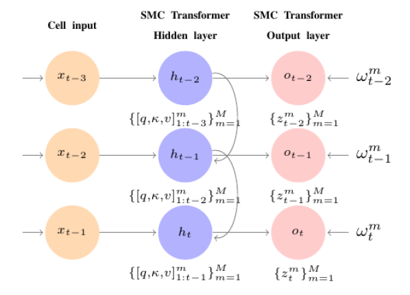
Figure 1: Graphical representation of the SMC transformer for sequential data.

3.2 The training algorithm

In this subsection, we detail how to train the stochastic self-attention model by estimating the objective function, i.e. the negative log-likelihood of the observations, using SMC methods. By section 3.1, the unobserved state at time $t$ is $\zeta_{t}=\{z(t),q(t),\kappa(t),v(t)\}$ and the complete-data likelihood may be written:

$$p_{\theta}(X_{1:T},\zeta_{1:T})=\prod_{t=1}^{T}p_{\theta}(\zeta_{t}|\zeta_{t-\Delta:t-1},X_{t-\Delta:t-1})p_{\theta}(X_{t}|\zeta_{t-\Delta:t},X_{t-\Delta:t-1})\,,$$

where by convention if $t-\Delta\leqslant 1$ then $u_{t-\Delta:s}=u_{1:s}$. The associated probability density function in the regression setting is:

$$p_{\theta}(X_{t}|\zeta_{t-\Delta:t},X_{t-\Delta:t-1})=\varphi_{G_{\eta_{obs}}(z(t)),\Sigma_{\mathrm{obs}}}(X_{t})\,,$$

where $\varphi_{\mu,\Sigma}$ is the Gaussian probability density function with mean $\mu$ and covariance matrix $\Sigma$. By (1) and (2), the sequential Monte Carlo algorithm approximates $\nabla_{\theta}\log p_{\theta}(X_{1:T})$ by a weighted sample mean:

$$S_{\theta,T}^{M}=\sum_{m=1}^{M}\omega_{T}^{m}\sum_{t=1}^{T}\big{[}\nabla_{\theta}\log p_{\theta}(\xi^{m}_{t}|\xi^{m}_{t-\Delta:t-1},X_{t-\Delta:t-1})+\nabla_{\theta}\log p_{\theta}(X_{t}|\xi^{m}_{t-\Delta:t},X_{t-\Delta:t-1})\big{]}\,,$$ (4)

where the importance weights $(\omega_{T}^{m})_{1\leqslant m\leqslant M}$ and the trajectories $\xi_{1:T}^{m}$ are sampled according to the particle filter described below. In this paper, we thus estimate the recurrent transformer parameters based on a gradient descent using $S_{\theta,T}^{M}$. All parameters related to the noise (i.e., covariance matrices) are estimated using an explicit Expectation Maximization (EM) update [Dempster et al., 1977] each time a batch of observations is processed as detailed in Appendix A.

Particle filtering/smoothing algorithm.

For all $t\geqslant 1$, once the observation $X_{t}$ is available, the weighted particle sample $\{(\omega_{t}^{m},\xi_{1:t}^{m})\}_{m=1}^{N}$ is transformed into a new weighted particle sample. This update step is carried through in two steps, selection and mutation, using the auxiliary sampler introduced in [Pitt and Shephard, 1999]. New indices and particles $\{(I_{t+1}^{m},\xi_{t+1}^{m})\}_{m=1}^{N}$ are simulated independently as follows:

1. Sample $I_{t+1}^{m}$ in $\{1,\ldots,N\}$ with probabilities proportional to $\{\omega_{t}^{j}\}_{1\leqslant j\leqslant N}$.

2. Sample $\xi_{t+1}^{m}$ using the model introduced in Section 3.1 with the resampled trajectories.

For any $m\in\{1,\dots,N\}$, the ancestral line is updated as follows $\xi_{1:t+1}^{m}=(\xi_{1:t}^{I_{t+1}^{m}},\xi_{t+1}^{m})$ and is associated with the importance weight defined by

$$\omega_{t+1}^{m}\propto p_{\theta}(X_{t+1}|\xi^{m}_{t+1-\Delta:t+1},X_{t+1-\Delta:t})\,.$$ (5)

Therefore, $\omega_{t+1}^{m}\propto\exp\{-\|X_{t+1}-G_{\eta_{obs}}(z_{t+1}^{m})\|^{2}_{\Sigma_{\mathrm{obs}}}/2\}$ in a regression setting.

This procedure introduced in [Kitagawa, 1996] (see also [Del Moral, 2004] for a discussion) approximates the joint smoothing distributions of the latent states given the observations using the genealogy of the particles produced by the auxiliary particle filter. The genealogical trajectories are defined recursively and updated at each time step with the particles and indices $(\xi^{m}_{k+1},I^{m}_{k+1})$. As a result, at each time step, the algorithm selects an ancestral trajectory by choosing its last state at time $k$, then extended using the newly sampled particle $\xi^{m}_{k+1}$.

Such algorithm, by maintaining a set of weighted particles and associated genealogical trajectories as an estimation of the SMC Transformer’s stochastic latent states, allows solving two usual objectives in state-space models: (i) the state estimation problem, which aims to recover the latent attention parameter $z_{t}$ at time $t$ given the observations $X_{1:t}$, and (ii) the inference problem which aims at approximating the distribution of $X_{t}$ given $X_{1:t-1}$. The next section focuses on the latter one, which provides a natural measure of uncertainty for the SMC Transformer predictions.

3.3 Inference and predictive distribution.

Given the parameter estimate $\widehat{\theta}$ obtained after the training phase, to solve the inference problem, note that

$$p_{\widehat{\theta}}(X_{t}|X_{1:t-1})=\int p_{\widehat{\theta}}(X_{t},z_{1:t}|X_{1:t-1})\mathrm{d}z_{1:t}\,,$$

which may be approximated using the weighted samples at time $t-1$ by

$$\widehat{p}^{M}_{\widehat{\theta}}(X_{t}|X_{1:t-1})=\sum_{m=1}^{M}\omega_{t-1}^{m}\int p_{\widehat{\theta}}(X_{t}|z_{t})p_{\widehat{\theta}}(z_{t}|\xi^{m}_{1:t-1},X_{1:t-1})\mathrm{d}z_{t}\,.$$

A Monte Carlo approximation of the predictive probability $\widehat{p}^{M}_{\widehat{\theta}}(X_{t}|X_{1:t-1})$ may be obtained straightforwardly by sampling from $p_{\widehat{\theta}}(z_{t}|\xi^{m}_{1:t-1},X_{1:t-1})$. With such estimate, we obtain as a predictive distribution a mixture $x_{t}\mapsto\sum_{m=1}^{M}\omega_{t-1}^{m}\varphi_{G_{\eta_{\mathrm{obs}}}(\hat{z}_{t}^{m}),\Sigma_{\mathrm{obs}}}(x_{t})$, where each mixture component $\hat{z}_{t}^{m}$ is sampled from $p_{\widehat{\theta}}(z_{t}|\xi^{m}_{1:t-1},X_{1:t-1})$, i.e. from one of the $M$ particles outputted by the SMC Transformer. Obtaining one sample $\hat{x}_{t}$ from this distribution amounts to (i) sampling a particle index $m$ with probabilities $\omega_{t-1}^{m}$, $1\leqslant m\leqslant M$, (ii) sampling $\hat{z}_{t}^{m}$ from $p_{\widehat{\theta}}(z_{t}|\xi^{m}_{1:t-1},X_{1:t-1})$, and (iii) sampling $\hat{x}_{t}$ from the Gaussian distribution with mean $G_{\eta_{\mathrm{obs}}}(\hat{z}_{t}^{m})$ and variance $\Sigma_{\mathrm{obs}}$. This Monte Carlo estimate can be extended straightforwardly to predictions at future time steps.

Such inference procedure is computationally efficient as it is based directly on the $M$ particles outputted by one single forward pass of the model on the test dataset. It also offers a flexible framework to estimate the predictive distribution. Indeed, the algorithm can be extended to more sophisticated estimation methods than a simple Monte Carlo estimate, that could improve both the predictive performance of the SMC Transformer, and its uncertainty estimation. We leave such a possibility for future works.

4 Experiments

4.1 Experimental Settings and Implementation details

To evaluate the performances of the SMC Transformer, we designed two experimental protocols. First, we create two synthetic datasets with known observation models: the goal is to assess whether the SMC Transformer can capture the true distribution of the observations. Second, we evaluate our model on several real-world datasets on time-series forecasting problems while measuring classic predictive intervals metrics.

For each experiment, we compare the SMC Transformer with the following baselines: a deterministic LSTM [Hochreiter and Schmidhuber, 1997] and transformer, a LSTM and transformer with MC Dropout [Gal and Ghahramani, 2015], and a Bayesian LSTM [Fortunato et al., 2017]. As mentioned in Section 3.1, we implement one-layer transformers with a single self-attention module, and the projection $G_{\eta_{obs}}$ is a point-wise feed-forward network with layer normalization [Ba et al., 2016] and residual connections as in [Ba et al., 2016]. To ensure full differentiability of the SMC Transformer’s algorithm, we applied the reparametrization trick [Kingma and Welling, 2014] on the Gaussian noises of the self-attention’s random variables. Additional details about datasets, models, and training algorithm’s hyper-parameters are provided in Appendix B.

4.2 Estimating the true variability of the observations on synthetic data

We design two synthetic auto-regressive time-series with a sequence length of 24 observations. For model I, one data sample $X=(X_{0},X_{1},...,X_{24})$ is drawn as follows, $X_{0}\sim\mathcal{N}(0,\,1)$ and for $t\geqslant 0$:

$$X_{t+1}=\alpha X_{t}+\sigma\varepsilon_{t+1}\,,$$

where $(\varepsilon_{t})_{1\leqslant t\leqslant 24}$ are i.i.d standard Gaussian variables independent of $X_{0}$. For model II, the law of a new observation given the past is multimodal and drawn as follows, $X_{0}\sim\mathcal{N}(0,\,1)$ and for $t\geqslant 0$:

$$X_{t+1}=\alpha U_{t+1}X_{t}+\beta(1-U_{t+1})X_{t}+\sigma\varepsilon_{t+1}\,,$$

where $(\varepsilon_{t})_{1\leqslant t\leqslant 24}$ are i.i.d standard Gaussian variables independent of $X_{0}$ and $(U_{t})_{1\leqslant t\leqslant 24}$ are i.i.d Bernoulli random variables with parameter $p$ independent of $X_{0}$ and of variance $(\varepsilon_{t})_{1\leqslant t\leqslant 24}$. In model I, the dataset is sampled with $\alpha=0.8$ and $\sigma^{2}=0.5$. In model II, the dataset is sampled with $\alpha=0.9$, $\beta=0.6\alpha$, $p=0.7$ and $\sigma^{2}=0.3$.

Table 1: Mean Square Error of the mean predictions (mse) and Mean Square Error of the predictive distribution (dist-mse) on the test set versus the ground truth, for Model I and II. Values are computed with a 5-fold cross-validation procedure on each dataset. Std values are displayed in parenthesis when stds $\geq 0.01.$. For the LSTM and Transformer models with MC Dropout, $p$ is the dropout rate. For the Bayesian LSTM, $M$ is the number of Monte Carlo samples to estimate the ELBO loss [Fortunato et al., 2017]. For the SMC Transformer, $M$ is the number of particles of the SMC algorithm.

Model	Model I		Model II
	mse	dist-mse	mse	dist-mse
True Model	0.5	0.50(0.03)	0.3	0.35(0.07)
LSTM	0.50	N.A	0.32	N.A
Transformer	0.52	N.A	0.32	N.A
LSTM drop.
$p=0.1$	0.48	0.004	0.32	0.003
$p=0.5$	0.53	0.03	0.33	0.02
Transf. drop.
$p=0.1$	0.50	0.02	0.31	0.03
$p=0.5$	0.52(0.01)	0.05(0.02)	0.33(0.02)	0.05(0.02)
Bayes. LSTM
$M=10$	0.53(0.01)	0.03	0.37(0.01)	0.04
SMC Transf.
$M=10$	0.52	0.49	0.30	0.35
$M=30$	0.49	0.52	0.34	0.35

Experimental results are summarized in Table 1 and Figure 2. Table 1 presents two metrics for the two synthetic models. First, we compute the Mean Square Error (mse) between the true observations and the predicted mean of the observations to measure the model predictive performance. For the SMC Transformer, this corresponds to the mean square error between the weighted mean over the particles’ predictions and the ground truth. Secondly, we refer as dist-mse, the empirical estimate of the mean square error of the predictive distribution of $X_{t+1}$ given the $\Delta$ past observations for all time steps $t$. Such an estimate is obtained by generating 1000 samples from the predictive distribution. For the SMC Transformer, they are drawn from the SMC estimate of the law of $X_{t+1}$ given $X_{0:t}$. For the baselines, they are drawn by performing 1000 stochastic forward passes on each data sample. For Model I, the dist-mse measure is given by $\mathbb{E}[(X_{t+1}-\alpha X_{t})^{2}|X_{t}]$, and the true value is $\sigma^{2}=0.5$. For Model II, the measure is $p\mathbb{E}[(X_{t+1}-\alpha X_{t})^{2}|X_{t}]+(1-p)\mathbb{E}[(X_{t+1}-\beta X_{t})^{2}|X_{t}]$, for which the true value is 0.35. In Table 1, we observe that all models perform similarly when predicting the mean of the observations. Yet, only the SMC Transformer manages to capture the true distribution of the observations accurately, with a dist-mse measure close to the ground truth. On the other side, both LSTM with MC Dropout and the Bayesian LSTM highly underestimate their variability, as illustrated by the small values of their dist-mse. Such findings are also illustrated in Figure 2. We there display the predictive distribution of the different methods versus the true 95% confidence interval given by the known observation model for the 24 timesteps of a test sample from Model I. Again, the SMC Transformer tends to match the true variability of the observations while concurrent methods clearly underestimate it.

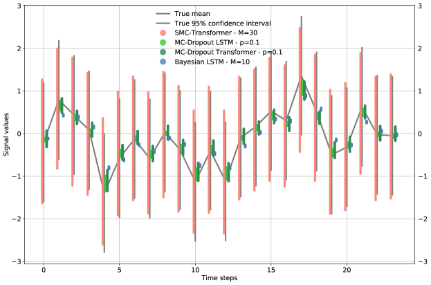
Figure 2: Samples distribution on a test example (Model I).

4.3 Predictive Intervals on real-world time-series.

The performance of the stochastic Transformer is evaluated on five real-world sequence predictions problems using the Covid-19, Jena weather, the GE stock datasets, and the air quality and energy consumption data from the UCI repository. Each dataset was split between a train dataset containing 70% of the data samples, and a validation and test sets containing an equal number of the remaining 15% of the data samples. Further dataset details are available in Appendix B.

For each of these time-series, we both perform unistep forecast and multistep forecast. Unistep forecast estimates the conditional distribution $p_{\widehat{\theta}}(X_{t}|X_{1:t-1})$ for every timestep of every test sample. The multistep forecast estimates the predictive distribution $p_{\widehat{\theta}}(X_{\tau_{H}+t}|X_{1:\tau_{H}})$, with $1\leqslant t\leqslant\tau_{F}$ on each test sample, given a frozen history of $\tau_{H}$ timesteps and a number $\tau_{F}$ future timesteps to predict.

Predictive intervals metrics.

In real-world time-series, we do not have access to the true distribution of the observations: we thus assess uncertainty by computing the Predicted Interval Coverage Percentage (PICP) [Pearce et al., 2018]. For any time step $t$ of the test set, a generative model can provide a lower and upper predicted interval (PI) bound, respectively $\hat{x}_{L_{t}}$ and $\hat{x}_{U_{t}}$ by sampling $M$ predictions of the predictive distribution at time $t$. The PICP [Pearce et al., 2018] of the true observations is then defined as:

$$\mathrm{PICP}=\frac{1}{n}\sum_{i=1}^{n}k_{i}\quad\mathrm{with}\quad k_{i}=\begin{cases}1&\text{if }\hat{x}_{L_{i}}\leqslant x_{i}\leqslant\hat{x}_{U_{i}}\,,\\ 0&\text{otherwise}\,,\end{cases}$$

where the mean is computed over all time steps considered in the test set. The Mean Predicted Interval Width (MPIW) is:

$$\mathrm{MPIW}=\frac{1}{n}\sum_{i=1}^{n}\left(\hat{x}_{U_{i}}-\hat{x}_{L_{i}}\right)\,.$$

If $\hat{x}_{L}$ and $\hat{y}_{U}$ represent the predictive bounds of a $(1-\alpha)$ confidence interval, intuitively, we want the associated $\mathrm{PICP}_{\alpha}$ to capture $1-\alpha$ proportion of the true observations, while having a corresponding $\mathrm{MPIW}_{\alpha}$ as small as possible.

Results.

Table 2 presents the tuple $(\mathrm{PICP}_{0.05},\mathrm{MPIW}_{0.05})$ associated with a 95% confidence interval when performing multistep forecasting on the five datasets. The unistep forecasting results are reported in Appendix B. Similarly to Section 4.1, we also report the mse over the test set between the mean predictions and the true observations. For $(\mathrm{PICP}_{0.05},\mathrm{MPIW}_{0.05})$, the highest $\mathrm{PICP}_{0.05}$ gives the best measure when it is lower than $0.95$; otherwise, the lowest $\mathrm{MPIW}_{0.05}$ gives the best measure, as proposed in [Pearce et al., 2018]. Additional results displaying the performances of the deterministic baselines, and others MC Dropout LSTM and Transformer variants are available in Appendix B.

Again, while all approaches present similar single-point estimate performances as illustrated with the mse values. The SMC Transformer outperforms the baselines in terms of $\mathrm{PICP}_{0.05}$ and $\mathrm{MPIW}_{0.05}$ for all datasets, except the energy consumption data, for which our approach is slightly outperformed by the MC Dropout LSTM with dropout rate equal to $0.1$.

Figure 3 represents the evolution of the $\mathrm{PICP}_{0.05}(t)$ per timestep $t$ when doing multistep forecasting for four of the five datasets: the SMC Transformer gives higher $\mathrm{PICP}_{0.05}(t)$ and tend to have a stabler PICP evolution over time than the concurrent baselines. Moreover, among the other approaches, there is no evident second best model for predicting uncertainty: sometimes the SMC Transformer is trailed by the MC Dropout Transformer, sometimes by the MC Dropout LSTM. The Bayesian LSTM tends to be particularly overconfident with PICP values often much lower than the ideal 95% threshold. As for the MC Dropout models, higher uncertainty measures (obtained generally with higher dropout rates) comes at the expense of predictive performance degradation. The discrepancy in uncertainty measures between the SMC Transformer and the baselines tends to be higher for datasets with longer sequences, suggesting that our approach is well-suited to model complex structured predictions problems with long-range dependencies. For instance, the stock dataset with a long temporal dependency of 40 past timesteps gives a gap of 11% between the SMC Transformer and the second best model. However, this gap is only equal to 1% for the energy dataset, which depends only on 12 past timesteps.

Table 2: mse (test loss), PICP and MPIW for multistep forecast. The values in bold correspond to the best performances for each metric.

	Covid		Air quality		Weather		Energy		Stock
	mse	picp — mpiw	mse	picp — mpiw	mse	picp — mpiw	mse	picp — mpiw	mse	picp — mpiw
LSTM drop.
$p=0.1$	0.150	0.67 — 0.61	0.139	0.54 — 0.73	0.089	0.62 — 1.15	0.07	0.96 — 1.12	0.065	0.85 — 0.74
$p=0.5$	0.155	0.80 — 1.64	0.211	0.70 — 1.31	0.157	0.75 — 1.74	0.218	0.88 — 1.57	0.112	0.87 — 1.42
Transf. drop.
$p=0.1$	0.121	0.74 — 0.74	0.141	0.69 — 1.44	0.127	0.38 — 0.59	0.046	0.89 — 0.60	0.076	0.71 — 0.54
$p=0.5$	0.208	0.84 — 1.52	0.196	0.77 — 1.97	0.180	0.59 — 1.04	0.09	0.94 — 1.21	0.106	0.83 — 0.77
Bayesian LSTM	0.144	0.15 — 0.23	0.192	0.49 — 0.72	0.092	0.27 — 0.38	0.121	0.93 — 1.08	0.086	0.34 — 0.45
SMC Transf.	0.128	0.91 — 1.85	0.148	0.97 — 3.17	0.180	0.92 — 2.90	0.043	0.97 — 1.33	0.071	0.98 — 1.80

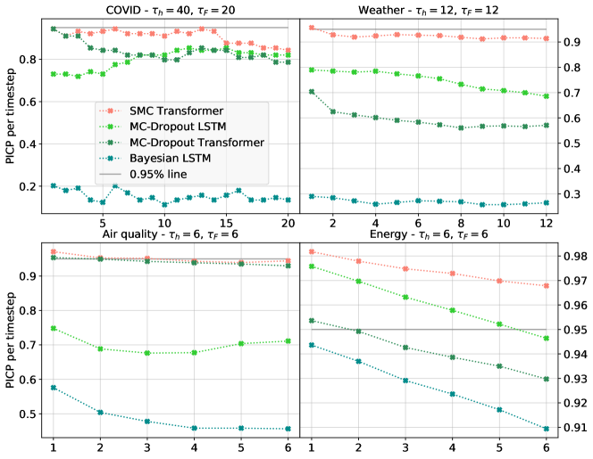
Figure 3: Plot of PICP per timestep when doing multi-step forecast for four of the five datasets. $\tau_{H}$ represents the number of past timesteps used to predict each of the $\tau_{F}$ future timesteps.

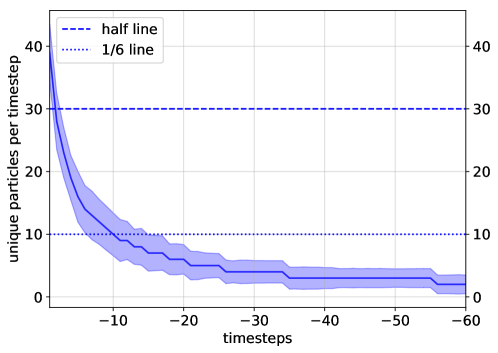
Figure 4: Evolution of the number of unique particles (or non-degenerated particles) over the past timesteps for the resampled trajectories $\xi^{m}_{t-\Delta:t-1}$ for a SMC Transformer with 60 particles, on the covid dataset. The timesteps are labeled from the most recent one ($t-1$, labeled as -1 on the figure), to the first timestep ($t-\Delta$, labeled as -60 on the figure). The straight line is the average number of particles over the predicted trajectories on the test set, while the shadow area is the corresponding 95% confidence interval.

4.4 Empirical study of the SMC algorithm: particles degeneracy

As highlighted in [Kitagawa, 1996, Kitagawa and Sato, 2001, Fearnhead et al., 2010, Poyiadjis et al., 2011], the particle smoother based on the genealogical trajectories suffers from the well known path degeneracy issue. At each time $t\geqslant 1$, the first step to build a new trajectory is to select an ancestral trajectory chosen among $M$ existing trajectories: as the number of resampling steps increases, the number of ancestral trajectories which are likely to be discarded increases.

In Figure 4, we illustrate this degeneracy phenomena on the covid dataset for a SMC Transformer with 60 particles. The figure displays the number of unique resampled trajectories $\xi^{m}_{t-\Delta:t-1}$ remaining for the 60 timesteps of the sequential process, averaged over the test set. The further we go in the past, the more the trajectories degenerate: for the first five timesteps, the trajectories are derived from only $2$ unique particles, and only the last ten timesteps present a set of unique particles whom size is superior to one sixth of the original size ($60$).

They are many solutions to improve the approximation $S_{\theta,T}^{M}$ and to avoid such phenomena. The easiest to implement is to use the fixed-lag smoother of [Olsson et al., 2008]: for each $1\leqslant t\leqslant n$, the trajectories $\xi^{m}_{t-\Delta:t-1}$ are only resampled up to a few time steps $\tau$ after $t$. Figure  4 indicates which value of $\tau$ should be used if we want to keep a sufficiently large number of unique past trajectories. Other approaches based on the decomposition of the smoothing distributions using backward kernels have been widely studied in the hidden Markov models literature [Doucet et al., 2000, Godsill et al., 2004, Del Moral et al., 2010, Olsson et al., 2017]. Extending such approaches to deep learning architectures at a reasonable computational cost is a practical challenge. We leave such improvement of the SMC algorithm in our generative model for future works.

5 Related work

Uncertainty estimation in Deep Learning has sparked a lot of interest from the research community over the last decade, leading to a rich literature on the subject. Such works are usually divided between frequentist approaches [Lakshminarayanan et al., 2017, Huang et al., 2017, Pearce et al., 2018, Tagasovska and Lopez-Paz, 2019, Wang et al., 2020, Osband et al., 2016] and Bayesian ones. Among the latter, Bayesian Neural Networks (BNNs) as defined in [Gal, 2016] put a prior distribution over the networks weights [Blundell et al., 2015, Gal and Ghahramani, 2015, Khan et al., 2018, Kendall et al., 2017, Teye et al., 2018, Hernández-Lobato and Adams, 2015]. However, they suffer from several limitations, one being their inability to correctly assess the posterior distribution [Foong et al., 2019] as illustrated in Section 4, the other being their computational overhead. Although MC Dropout is one of the most scalable Bayesian inference algorithms, its sampling procedure at inference, that relies on one stochastic forward pass per sample from the predictive distribution, is more computationally expensive than the SMC Transformer, for which sampling comes from a Gaussian mixture model directly derived from the particles predictions. Another Bayesian approach uses neural networks with stochastic hidden states as described below.

RNNs with stochastic latent states.

The SMC Transformer is part of an emerging line of research bridging state-space models (historically restricted to simpler statistical models such as Hidden Markov Models or Gaussian Linear Models) and Deep Neural Networks. A few works have proposed recurrent neural networks with stochastic latent states, such as VRAE [Fabius and van Amersfoort, 2015], VRNN [Chung et al., 2015], SRNN [Fraccaro et al., 2016], or VHRNN [Deng et al., 2020]. They use training algorithms that rely on variational inference methods [Blei et al., 2017] to approximate the intractable posterior distribution over the latent states. Such learning procedures are popular and are computationally efficient, but output a predictive distribution known to be ill-fitted for estimating certain families of distributions, such as for instance multimodal distributions.

SMC methods and RNNs.

Several SMC algorithms have then been developed to get a better estimator of the marginal likelihood of the observations for such stochastic RNNs, again in a variational inference framework. [Le et al., 2018, Naesseth et al., 2018, Maddison et al., 2017] proposed particle filtering algorithms, while [Lawson et al., 2018, Moretti et al., 2019] developed particle smoothing ones. Our work differs from the models and algorithms mentioned above in several ways. First, the training algorithm of the SMC Transformer relies on the Fisher’s Identity to estimate the gradient of the likelihood of the observations, instead of a variational objective. Secondly, this is the only work proposing: (i) a novel recurrent generative model based on a stochastic self-attention model, and (ii) a novel SMC algorithm to estimate the posterior distribution of the unobserved states, with resampling weights directly depending on the output of the SMC Transformer. Finally, while the above works only leverage the SMC algorithm to get a better and lower-variance estimator of the marginal log-likelihood, our work and evaluation protocol focus on uncertainty measurements for sequence prediction problems.

6 Conclusion

In this paper, we proposed the SMC Transformer, a novel recurrent network that naturally captures the distribution of the observations. This model maintains a distribution of self-attention parameters as latent states, estimated by a set of particles. It thus outputs a distribution of predictions instead of a single-point estimate. Our inference method gives a flexible framework to quantify the variability of the observations. To our knowledge, this is the first method dedicated to estimating uncertainty in the transformer model, and one of the few focusing on uncertainty quantification in the context of sequence prediction. Moreover, this SMC Transformer layer could be used as a ”plug-and-play” layer for uncertainty quantification in a deeper neural network encoding sequential data. One limitation of our model is its computational overhead at training time; yet, it can be eased using in particular variants of the SMC algorithm mentioned in section 4.4.

Appendix A Details on the training algorithm

Particle filtering/smoothing algorithm.

For all $t\geqslant 1$, once the observation $X_{t}$ is available, the weighted particle sample $\{(\omega_{t}^{m},\xi_{1:t}^{m})\}_{m=1}^{N}$ is transformed into a new weighted particle sample. This update step is carried through in two steps, selection and mutation, using the following sampler, see for instance [Pitt and Shephard, 1999]. New indices and particles $\{(I_{t+1}^{m},\xi_{t+1}^{m})\}_{m=1}^{N}$ are simulated independently as follows:

1. Sample $I_{t+1}^{m}$ in $\{1,\ldots,N\}$ with probabilities proportional to $\{\omega_{t}^{j}\}_{1\leqslant j\leqslant N}$.

2. Sample $\xi_{t+1}^{m}$ using the model with the resampled trajectories.

In the regression framework of the paper, for any $m\in\{1,\dots,N\}$, the ancestral line $\xi_{1:t+1}^{\ell}$ is updated as follows $\xi_{1:t+1}^{m}=(\xi_{1:t}^{I_{t+1}^{m}},\xi_{t+1}^{m})$ and is associated with the importance weight defined by

$$\omega_{t+1}^{m}\propto p_{\theta}(X_{t+1}|\xi^{m}_{t+1-\Delta:t+1},X_{t+1-\Delta:t})=\exp\{-\|X_{t+1}-G_{\eta_{obs}}(z_{t+1}^{m})\|^{2}_{\Sigma_{\mathrm{obs}}}/2\}\,,$$

where $\|X_{t+1}-G_{\eta_{obs}}(z_{t+1}^{m})\|^{2}_{\Sigma_{\mathrm{obs}}}=(X_{t+1}-G_{\eta_{obs}}(z_{t+1}^{m}))^{\top}\Sigma_{\mathrm{obs}}^{-1}(X_{t+1}-G_{\eta_{obs}}(z_{t+1}^{m}))$. The algorithm is illustrated in Figure 5: particles at the last time step are in blue and pink particles are the ones which appear in the genealogy of at least one blue particle. White particle have not been selected to give birth to a path up to the last time. In Figure 5, the $N=3$ genealogical trajectories are $\xi^{1}_{0:4}=(\xi_{0}^{3},\xi_{1}^{2},\xi_{2}^{2},\xi_{3}^{3},\xi_{4}^{1})$, $\xi^{2}_{0:4}=(\xi_{0}^{3},\xi_{1}^{1},\xi_{2}^{3},\xi_{3}^{2},\xi_{4}^{2})$, $\xi^{3}_{0:4}=(\xi_{0}^{3},\xi_{1}^{2},\xi_{2}^{2},\xi_{3}^{3},\xi_{4}^{3})$.

Figure 5: Particle filter: $N=3$, $n=4$.

The training algorithm

The sequential Monte Carlo algorithm approximates $\nabla_{\theta}\log p_{\theta}(X_{1:T})$ by a weighted sample mean:

$$S_{\theta,T}^{M}=\sum_{m=1}^{M}\omega_{T}^{m}\sum_{t=1}^{T}\left[\nabla_{\theta}\log p_{\theta}(\xi^{m}_{t}|\xi^{m}_{t-\Delta:t-1},X_{t-\Delta:t-1})+\nabla_{\theta}\log p_{\theta}(X_{t}|\xi^{m}_{t-\Delta:t},X_{t-\Delta:t-1})\right]\,,$$

where the importance weights $(\omega_{T}^{m})_{1\leqslant m\leqslant M}$ and the trajectories $\xi_{1:T}^{m}$ are sampled according to the particle filter described below. Thanks to Fisher’s identity, this approximation only requires to compute the gradient of state model $\theta\mapsto\log p_{\theta}(\xi^{m}_{t}|\xi^{m}_{t-\Delta:t-1},X_{t-\Delta:t-1})$ and the gradient of the observation model $\theta\mapsto\log p_{\theta}(X_{t}|\xi^{m}_{t-\Delta:t},X_{t-\Delta:t-1})$. There is no need to compute the gradient of the weights $\omega_{T}^{m}$ which depend on the parameter $\theta$. The loss function used to train the model is therefore

$$\theta\mapsto-\sum_{m=1}^{M}\omega_{T}^{m}\sum_{t=1}^{T}\left[\log p_{\theta}(\xi^{m}_{t}|\xi^{m}_{t-\Delta:t-1},X_{t-\Delta:t-1})+\log p_{\theta}(X_{t}|\xi^{m}_{t-\Delta:t},X_{t-\Delta:t-1})\right]\,.$$

In this paper, we propose to estimate all the parameters of the recurrent architecture based on a gradient descent using $S_{\theta,T}^{M}$. All parameters related to the noise (the covariance matrices) are estimated using an explicit Expectation Maximization (EM) update [Dempster et al., 1977] each time a batch of observations is processed, see the supplementary materials for all details. For each sequence of observations, the EM update relies on the approximation of the intermediate quantity

$$\mathbb{E}[\log p_{\theta}(X_{1:T},\zeta_{1:T})|X_{1:T}]=\sum_{t=1}^{T}\mathbb{E}[\log p_{\theta}(\zeta_{t}|\zeta_{t-\Delta:t-1},X_{t-\Delta:t-1})+\log p_{\theta}(X_{t}|\zeta_{t-\Delta:t},X_{t-\Delta:t-1})|X_{1:T}]$$

by the following particle-based estimator:

$$Q_{\theta,T}^{M}=\sum_{m=1}^{M}\omega_{T}^{m}\sum_{t=1}^{T}\left[\log p_{\theta}(\xi^{m}_{t}|\xi^{m}_{t-\Delta:t-1},X_{t-\Delta:t-1})+\log p_{\theta}(X_{t}|\xi^{m}_{t-\Delta:t},X_{t-\Delta:t-1})\right]\,.$$

Then, $Q_{\theta,T}^{M}$ may be maximized with respect to all covariances to obtain the new estimates. This is a straightforward update which yields for instance for $\Sigma_{\mathrm{obs}}$ for the $p$-th update:

$$\Sigma^{p}_{\mathrm{obs}}=\frac{1}{T}\sum_{m=1}^{M}\omega_{T}^{m}\sum_{t=1}^{T}(X_{t}-G_{\eta_{obs}}(r_{t}^{m}))^{\top}(X_{t}-G_{\eta_{obs}}(r_{t}^{m}))\,,$$

where $r_{t}^{m}$ are the resampled particles at time $t$. The new estimate of $\Sigma_{\mathrm{obs}}$ is then

$$\widehat{\Sigma}_{\mathrm{obs}}=(1-\eta_{p})\widehat{\Sigma}_{\mathrm{obs}}+\eta_{p}\Sigma^{p}_{\mathrm{obs}}\,$$

where $\eta_{p}$ is a learning rate chosen by the user ($\eta_{p}=p^{-0.6}$ in the experiments).

Appendix B Experiments

B.1 Baselines

The LSTM and Transformer with MC Dropout [Gal and Ghahramani, 2015] have respectively one and two dropout layers. For the LSTM, this layer is just before the output layer. For the Transformer, the dropout layers are inserted in the network architecture as in [Vaswani et al., 2017]. The first dropout layer is after the attention module that computes the output attention vector, and the second one is just before the last layer-normalization layer of the feed-forward neural network that transforms the attention vector. The same dropout rate is kept during training and inference.

The implementation of the Bayesian LSTM relies on the blitz library, following the model from [Fortunato et al., 2017]. On the synthetic setting, a hyper-parameter search was performed on $\mathrm{prior_{\sigma_{1}}}$, the standard deviation of the first component of the gaussian mixture model that models the prior distribution over the network’s weights, and on $\mathrm{prior}_{\pi}$, the factor to scale this mixture model, as follows:

$$\mathrm{prior_{\sigma_{1}}}\in\{0.1,0.135,0.37,0.75,1,1.5\},\quad\mathrm{prior}_{\pi}\in\{0.25,0.5,0.75,1\}\,.$$

The best results in terms of predictive performance were obtained for $\mathrm{prior_{\sigma_{1}}}=0.1$ and $\mathrm{prior_{\sigma_{1}}}=1$: we kept these values for the experiments on the real-world datasets. The other hyper-parameters of the Bayesian LSTM were kept at the default values provided by the blitz library.

B.2 Hyper-parameters

Models dimensions.

The LSTM models (deterministic LSTM, MC Dropout LSTM, Bayesian LSTM) have a number of units in the recurrent layer equal to $32$. The Transformer models (deterministic Transformer, MC Dropout Transformer, and SMC Transformer) have a depth (dimension of the attention parameters) equal to $32$, and a number of units in the feed-forward neural network that transforms the attention vector also equal to $32$.

Training hyper-parameters.

For training the SMC Transformer and the baselines, we use the ADAM algorithm with a learning rate of 0.001 for the LSTM networks and the original custom schedule found in [Vaswani et al., 2017] for the Transformer networks. Models were trained for 50 epochs, except the Bayesian LSTM that was trained for 150 epochs. For the two synthetic models, a batch size of $32$ was used. On the real-world setting, batch sizes of 32, 64, 256, 128 and 64 were respectively used for the covid, air quality, weather, energy and stock datasets.

B.3 Datasets

Synthetic data.

The synthetic datasets were generated with 1000 samples: we used 800 of them for training and 100 of them for test and validation. A 5-fold cross-validation procedure was performed at training, to estimate the variability in performance that can be attributed to the training algorithm (by opposition with the measurement of the observations variability, computed with the dist-mse metric described in Section 4.2 of the main paper).

Real-world time series.

We use a 0.7 / 0.15 / 0.15 split for training, validation and test for the real-world datasets.

The covid dataset is a univariate time series gathering the daily deaths from the covid-19 disease in 3261 US cities. Cities with less than 100 deaths over the time period considered were discarded from the dataset, leading to 886 samples in the final dataset, with a sequence length equal to $60$, corresponding to 2 months of observations.

The air quality dataset gathers hourly responses of a gas multisensor device deployed in an Italian city. It is a multivariate time series with 9 input features: we kept 5 features as target features to be predicted, corresponding to the concentration of 5 chemical gases in the atmosphere. The final dataset has $9,348$ samples, and a sequence length equal to $12$, corresponding to a half day of observations.

The weather dataset gathers meteorological data from a German weather station. It is a multivariate time series with 4 input and target features (temperature, air pressure, relative humidity, and air density). The final dataset have $420,551$ samples, and a sequence length equal to $24$, corresponding to one day of observations.

The energy dataset gathers 10-min measurements of household appliances energy consumption, coupled with local meteorological data. It is a multivariate time series with 28 input features: we kept 20 target features to be predicted. The final dataset have $19,735$ samples, and a sequence length equal to $12$, corresponding to 2 hours of observations.

The stock dataset gathers daily stock prices and volume of General Electric stocks. It is a multivariate time series with 5 input features. The final dataset have $3,020$ samples, and a sequence length equal to $40$, corresponding to 2 months of observations (recorded only during business days).

B.4 Additional results

Table 3 presents additional results on the synthetic datasets, and displays the mse and dist-mse described in section 4.2 of the main paper.

Table 4 and Table 5 present the additional results when doing respectively unistep forecasting and multi-step forecasting, and display the mean square error over the test set, and the predictive interval metrics (PICP and MPIW) described in section 4.3 of the main paper. For the multivariate time series, the PICP and MPIW are averaged over all the target features.

Table 3: Mean Square Error of the mean predictions (mse) and Mean Square Error of the predictive distribution (dist-mse) on the test set versus the ground truth, for Model I and II. Values are computed with a 5-fold cross-validation procedure on each dataset. Std values are displayed in parenthesis when stds $\geq 0.01.$. For the LSTM and Transformer models with MC Dropout, $p$ is the dropout rate. For the Bayesian LSTM, $M$ is the number of Monte Carlo samples to estimate the ELBO loss [Fortunato et al., 2017]. We display the results for $M=3$, as it is the default parameter value provided by the blitz library. For the SMC Transformer, $M$ is the number of particles of the SMC algorithm.

Model	Model I		Model II
	mse	dist-mse	mse	dist-mse
True Model	0.5	0.50(0.03)	0.3	0.35(0.07)
LSTM	0.50	N.A	0.32	N.A
Transformer	0.52	N.A	0.32	N.A
LSTM drop.
$p=0.1$	0.48	0.004	0.32	0.003
$p=0.2$	0.53	0.0099	0.34	0.007
$p=0.5$	0.53	0.03	0.33	0.02
Transf. drop.
$p=0.1$	0.50	0.02	0.31	0.03
$p=0.2$	0.50	0.02(0.01)	0.32	0.02
$p=0.5$	0.52(0.01)	0.05(0.02)	0.33(0.02)	0.05(0.02)
Bayes. LSTM
$M=3$	0.55(0.01)	0.04	0.36(0.01)	0.05
$M=10$	0.53(0.01)	0.03	0.37(0.01)	0.04
SMC Transf.
$M=10$	0.52	0.49	0.30	0.35
$M=30$	0.49	0.52	0.34	0.35

Table 4: mse (test loss), PICP and MPIW for unistep forecast. The values in bold correspond to the best performances for each metric.

	Covid		Air quality		Weather		Energy		Stock
	mse	picp — mpiw	mse	picp — mpiw	mse	picp — mpiw	mse	picp — mpiw	mse	picp — mpiw
LSTM	0.117	- — -	0.120	- — -	0.076	- — -	0.039	- — -	0.055	- — -
LSTM drop.
$p=0.1$	0.150	0.77 — 0.27	0.139	0.64 — 0.40	0.089	0.55 — 0.38	0.07	0.99 — 0.49	0.065	0.93 — 0.28
$p=0.2$	0.159	0.79 — 0.38	0.152	0.72 — 0.54	0.101	0.64 — 0.53	0.103	0.99— 0.45	0.074	0.95 — 0.38
$p=0.5$	0.155	0.89 — 0.63	0.211	0.86 — 0.87	0.157	0.78 — 0.92	0.218	0.96 — 1.24	0.112	0.97 — 0.108
Transf.	0.116	- — -	0.132	- — -	0.099	- — -	0.042	- — -	0.068	- — -
Transf drop.
$p=0.1$	0.121	0.96 — 0.37	0.141	0.77 — 0.47	0.127	0.60 — 0.35	0.046	0.96 — 0.45	0.076	0.93 — 0.34
$p=0.2$	0.129	0.94 — 0.46	0.159	0.89 — 0.58	0.133	0.72 — 0.44	0.053	0.98 — 0.64	0.082	0.95 — 0.41
$p=0.5$	0.208	0.97 — 0.76	0.196	0.96 — 0.85	0.180	0.89 — 0.68	0.09	0.97 — 1.00	0.106	0.95 — 0.63
Bayesian LSTM	0.144	0.25 — 0.12	0.192	0.77 — 0.51	0.092	0.25 — 0.15	0.121	0.91 — 0.76	0.086	0.85 — 0.22
SMC Transf.	0.128	0.997 — 0.70	0.148	0.97 — 1.54	0.180	0.99 — 1.65	0.043	0.99 — 0.82	0.071	0.99 — 1.08

Table 5: mse (test loss), PICP and MPIW for multistep forecast. The values in bold correspond to the best performances for each metric.

	Covid		Air quality		Weather		Energy		Stock
	mse	picp — mpiw	mse	picp — mpiw	mse	picp — mpiw	mse	picp — mpiw	mse	picp — mpiw
LSTM drop.
$p=0.1$	0.150	0.67 — 0.61	0.139	0.54 — 0.73	0.089	0.62 — 1.15	0.07	0.96 — 1.12	0.065	0.85 — 0.74
$p=0.2$	0.159	0.73 — 0.83	0.152	0.60 — 0.97	0.101	0.70 — 1.44	0.07	0.96 — 1.12	0.065	0.85 — 0.74
$p=0.5$	0.155	0.80 — 1.64	0.211	0.70 — 1.31	0.157	0.75 — 1.74	0.218	0.88 — 1.57	0.112	0.87 — 1.42
Transf. drop.
$p=0.1$	0.121	0.74 — 0.74	0.141	0.69 — 1.44	0.127	0.38 — 0.59	0.046	0.89 — 0.60	0.076	0.71 — 0.54
$p=0.2$	0.129	0.73 — 0.77	0.152	0.60 — 0.97	0.101	0.70 — 1.44	0.053	0.93 — 0.77	0.082	0.71 — 0.54
$p=0.5$	0.208	0.84 — 1.52	0.196	0.77 — 1.97	0.180	0.59 — 1.04	0.09	0.94 — 1.21	0.106	0.83 — 0.77
Bayesian LSTM	0.144	0.15 — 0.23	0.192	0.49 — 0.72	0.092	0.27 — 0.38	0.121	0.93 — 1.08	0.086	0.34 — 0.45
SMC Transf.	0.128	0.91 — 1.85	0.148	0.97 — 3.17	0.180	0.92 — 2.90	0.043	0.97 — 1.33	0.071	0.98 — 1.80

References

- [Ashukha et al., 2020] Ashukha, A., Lyzhov, A., Molchanov, D., and Vetrov, D. (2020). Pitfalls of in-domain uncertainty estimation and ensembling in deep learning. In International Conference on Learning Representations (ICLR).
- [Ba et al., 2016] Ba, J. L., Kiros, J. R., and Hinton, G. E. (2016). Layer normalization. arXiv preprint arXiv:1607.06450.
- [Bahdanau et al., 2015] Bahdanau, D., Cho, K., and Bengio, Y. (2015). Neural machine translation by jointly learning to align and translate. In Proceedings of the International Conference on Learning Representations (ICLR).
- [Blei et al., 2017] Blei, D. M., Kucukelbir, A., and McAuliffe, J. D. (2017). Variational inference: A review for statisticians. Journal of the American statistical Association, 112(518):859–877.
- [Blundell et al., 2015] Blundell, C., Cornebise, J., Kavukcuoglu, K., and Wierstra, D. (2015). Weight uncertainty in neural networks. Proceedings of the International Conference on Machine Learning (ICML).
- [Campbell et al., 2000] Campbell, C., Cristianini, N., and Smola, A. J. (2000). Query learning with large margin classifiers. In Proceedings of International Conference on Machine Learning (ICML).
- [Cappé et al., 2005] Cappé, O., Moulines, E., and Rydén, T. (2005). Inference in Hidden Markov Models. Springer.
- [Chung et al., 2015] Chung, J., Kastner, K., Dinh, L., Goel, K., Courville, A. C., and Bengio, Y. (2015). A recurrent latent variable model for sequential data. In Proceedings of the Advances in Neural Information Processing Systems (NIPS).
- [Del Moral, 2004] Del Moral, P. (2004). Feynman-Kac Formulae: Genealogical and Interacting Particle Systems With Applications. Springer.
- [Del Moral et al., 2010] Del Moral, P., Doucet, A., and Singh, S. S. (2010). A backward particle interpretation of feynman-kac formulae. ESAIM: Mathematical Modelling and Numerical Analysis, 44(5):947–975.
- [Dempster et al., 1977] Dempster, A. P., Laird, N. M., and Rubin, D. B. (1977). Maximum likelihood from incomplete data via the EM algorithm. Journal of the Royal Statistical Society: Series B, 39(1):1–38.
- [Deng et al., 2020] Deng, R., Cao, Y., Chang, B., Sigal, L., Mori, G., and Brubaker, M. A. (2020). Variational hyper rnn for sequence modeling. arXiv preprint arXiv:2002.10501.
- [Devlin et al., 2019] Devlin, J., Chang, M.-W., Lee, K., and Toutanova, K. (2019). Bert: Pre-training of deep bidirectional transformers for language understanding. Proceedings of the Conference of the North American Chapter of the Association for Computational Linguistics (NAACL).
- [Doucet et al., 2000] Doucet, A., Godsill, S., and Andrieu, C. (2000). On sequential Monte-Carlo sampling methods for Bayesian filtering. Statistics and Computing, 10:197–208.
- [Dubarry and Le Corff, 2013] Dubarry, C. and Le Corff, S. (2013). Non-asymptotic deviation inequalities for smoothed additive functionals in nonlinear state-space models. Bernoulli, 19(5B):2222–2249.
- [Fabius and van Amersfoort, 2015] Fabius, O. and van Amersfoort, J. R. (2015). Variational recurrent auto-encoders. In Workshop of the International Conference on Learning Representations (ICLR).
- [Fearnhead et al., 2010] Fearnhead, P., Wyncoll, D., and Tawn, J. (2010). A sequential smoothing algorithm with linear computational cost. Biometrika, 97(2):447–464.
- [Foong et al., 2019] Foong, A. Y., Burt, D. R., Li, Y., and Turner, R. E. (2019). On the expressiveness of approximate inference in bayesian neural networks. arXiv preprint arXiv:1909.00719.
- [Fortunato et al., 2018] Fortunato, M., Azar, M. G., Piot, B., Menick, J., Osband, I., Graves, A., Mnih, V., Munos, R., Hassabis, D., Pietquin, O., Blundell, C., and Legg, S. (2018). Noisy networks for exploration. In Proceedings of the International Conference on Representation Learning (ICLR).
- [Fortunato et al., 2017] Fortunato, M., Blundell, C., and Vinyals, O. (2017). Bayesian recurrent neural networks. arXiv preprint arXiv:1704.02798.
- [Fraccaro et al., 2016] Fraccaro, M., Sønderby, S. K., Paquet, U., and Winther, O. (2016). Sequential neural models with stochastic layers. In Proceedings of the Advances in Neural Information Processing Systems (NIPS).
- [Gal, 2016] Gal, Y. (2016). Uncertainty in deep learning. University of Cambridge, 1(3).
- [Gal and Ghahramani, 2015] Gal, Y. and Ghahramani, Z. (2015). Dropout as a bayesian approximation: Representing model uncertainty in deep learning. In Proceedings of the International Conference on Machine Learning (ICML).
- [Geist and Pietquin, 2010] Geist, M. and Pietquin, O. (2010). Kalman temporal differences. Journal of artificial intelligence research, 39:483–532.
- [Godsill et al., 2004] Godsill, S. J., Doucet, A., and West, M. (2004). Monte Carlo smoothing for non-linear time series. Journal of the American Statistical Association, 50:438–449.
- [Gordon et al., 1993] Gordon, N., Salmond, D., and Smith, A. (1993). Novel approach to nonlinear/non-Gaussian bayesian state estimation. Proceedings of the IEEE Conference of Radar Signal Process.
- [Hernández-Lobato and Adams, 2015] Hernández-Lobato, J. M. and Adams, R. (2015). Probabilistic backpropagation for scalable learning of bayesian neural networks. In Proceedings of the International Conference on Machine Learning (ICML).
- [Hochreiter and Schmidhuber, 1997] Hochreiter, S. and Schmidhuber, J. (1997). Long short-term memory. Neural computation, 9(8):1735–1780.
- [Huang et al., 2017] Huang, G., Li, Y., Pleiss, G., Liu, Z., Hopcroft, J. E., and Weinberger, K. Q. (2017). Snapshot ensembles: Train 1, get M for free. In Proceedings of the International Conference on Learning Representations (ICLR).
- [Igl et al., 2018] Igl, M., Zintgraf, L., Le, T. A., Wood, F., and Whiteson, S. (2018). Deep variational reinforcement learning for pomdps. In Proceedings of the International Conference on Machine Learning (ICML).
- [Kendall et al., 2017] Kendall, A., Badrinarayanan, V., and Cipolla, R. (2017). Bayesian segnet: Model uncertainty in deep convolutional encoder-decoder architectures for scene understanding. In British Machine Vision Conference 2017, BMVC 2017, London, UK, September 4-7, 2017. BMVA Press.
- [Khan et al., 2018] Khan, M. E., Nielsen, D., Tangkaratt, V., Lin, W., Gal, Y., and Srivastava, A. (2018). Fast and scalable bayesian deep learning by weight-perturbation in adam. In Proceedings of the International Conference on Machine Learning (ICML).
- [Kingma and Welling, 2014] Kingma, D. P. and Welling, M. (2014). Auto-encoding variational bayes. In Proceedings of the International Conference on Learning Representations (ICLR).
- [Kitagawa, 1996] Kitagawa, G. (1996). Monte-Carlo filter and smoother for non-Gaussian nonlinear state space models. Journal of Computational and Graphical Statistics, 1:1–25.
- [Kitagawa and Sato, 2001] Kitagawa, G. and Sato, S. (2001). Monte carlo smoothing and self-organizing state-space model. In Doucet, A., De Freitas, N., and Gordon, N., editors, Sequential Monte Carlo methods in Practice. Springer.
- [Lakshminarayanan et al., 2017] Lakshminarayanan, B., Pritzel, A., and Blundell, C. (2017). Simple and scalable predictive uncertainty estimation using deep ensembles. In Proceedings of the Advances in Neural Information Processing Systems (NIPS).
- [Lawson et al., 2018] Lawson, D., Tucker, G., Naesseth, C. A., Maddison, C. J., Adams, R. P., and Teh, Y. W. (2018). Twisted variational sequential monte carlo. In Third workshop on Bayesian Deep Learning (NeurIPS).
- [Le et al., 2018] Le, T. A., Igl, M., Rainforth, T., Jin, T., and Wood, F. (2018). Auto-encoding sequential monte carlo. In Proceedings of the International Conference on Learning Representations (ICLR).
- [Li et al., 2019] Li, S., Jin, X., Xuan, Y., Zhou, X., Chen, W., Wang, Y.-X., and Yan, X. (2019). Enhancing the locality and breaking the memory bottleneck of transformer on time series forecasting. In Proceedings of the Advances in Neural Information Processing Systems.
- [Lin et al., 2014] Lin, Z., Feng, M., dos Santos, C. N., Yu, M., Xiang, B., Zhou, B., and Bengio, Y. (2014). A structured self-attentive sentence embedding. In Proceedings of the International Conference on Learning Representations (ICLR).
- [Liu and Chen, 1998] Liu, J. and Chen, R. (1998). Sequential Monte Carlo methods for dynamic systems. Journal of the American Statistical Association, 93:1032–1044.
- [MacKay, 1992] MacKay, D. J. (1992). A practical bayesian framework for backpropagation networks. Neural computation, 4(3):448–472.
- [Maddison et al., 2017] Maddison, C. J., Lawson, J., Tucker, G., Heess, N., Norouzi, M., Mnih, A., Doucet, A., and Teh, Y. (2017). Filtering variational objectives. In Proceedings of Advances in Neural Information Processing Systems (NIPS).
- [Moretti et al., 2019] Moretti, A. K., Wang, Z., Wu, L., Drori, I., and Pe’er, I. (2019). Particle smoothing variational objectives. arXiv preprint arXiv:1909.09734.
- [Naesseth et al., 2018] Naesseth, C., Linderman, S., Ranganath, R., and Blei, D. (2018). Variational sequential monte carlo. In Proceedings of the International Conference on Artificial Intelligence and Statistics (AISTATS).
- [Neal, 2012] Neal, R. M. (2012). Bayesian learning for neural networks, volume 118. Springer Science & Business Media.
- [Olsson et al., 2008] Olsson, J., Cappe, O., Douc, R., and Moulines, E. (2008). Sequential monte carlo smoothing with application to parameter estimation in nonlinear state space models. Bernoulli, 14(1):155–179.
- [Olsson et al., 2017] Olsson, J., Westerborn, J., et al. (2017). Efficient particle-based online smoothing in general hidden Markov models: the PaRIS algorithm. Bernoulli, 23(3):1951–1996.
- [Osband et al., 2016] Osband, I., Blundell, C., Pritzel, A., and Van Roy, B. (2016). Deep exploration via bootstrapped dqn. In Proceedings of the Advances in Neural Information Processing Systems (NIPS).
- [Pearce et al., 2018] Pearce, T., Brintrup, A., Zaki, M., and Neely, A. (2018). High-quality prediction intervals for deep learning: A distribution-free, ensembled approach. In Proceedings of the International Conference on Machine Learning (ICML).
- [Pitt and Shephard, 1999] Pitt, M. K. and Shephard, N. (1999). Filtering via simulation: Auxiliary particle filters. Journal of the American Statistical Association, 94(446):590–599.
- [Poyiadjis et al., 2011] Poyiadjis, G., Doucet, A., and Singh, S. (2011). Particle approximations of the score and observed information matrix in state space models with application to parameter estimation. Biometrika, 98:65–80.
- [Tagasovska and Lopez-Paz, 2019] Tagasovska, N. and Lopez-Paz, D. (2019). Single-model uncertainties for deep learning. In Proceedings of the Advances in Neural Information Processing Systems (NeurIPS).
- [Teye et al., 2018] Teye, M., Azizpour, H., and Smith, K. (2018). Bayesian uncertainty estimation for batch normalized deep networks. In Proceedings of the International Conference on Machine Learning (ICML).
- [Vaswani et al., 2017] Vaswani, A., Shazeer, N., Parmar, N., Uszkoreit, J., Jones, L., Gomez, A. N., Kaiser, Ł., and Polosukhin, I. (2017). Attention is all you need. In Proceedings of the Advances in Neural Information Processing Systems (NIPS).
- [Wang et al., 2020] Wang, B., Li, T., Yan, Z., Zhang, G., and Lu, J. (2020). Deeppipe: A distribution-free uncertainty quantification approach for time series forecasting. Neurocomputing.
- [Zhu and Laptev, 2017] Zhu, L. and Laptev, N. (2017). Deep and confident prediction for time series at uber. In Proceedings of the IEEE International Conference on Data Mining Workshops (ICDMW).