Black holes in torsion bigravity

Abstract

We study spherically symmetric black hole solutions in a four-parameter Einstein-Cartan-type class of theories, called “torsion bigravity”. These theories offer a geometric framework (with a metric and an independent torsionfull connection) for a modification of Einstein’s theory that has the same spectrum as bimetric gravity models. In addition to an Einsteinlike massless spin-2 excitation, there is a massive spin-2 one (of range $\kappa^{-1}$) coming from the torsion sector, rather than from a second metric. We prove the existence of three broad classes of spherically-symmetric black hole solutions in torsion bigravity. First, the Schwarzschild  solution defines an asymptotically-flat torsionless black hole for all values of the parameters. [And we prove that one cannot deform a Schwarzschild  solution, at the linearized level, by adding an infinitesimal torsion hair.] Second, when considering finite values of the range, we find that there exist non-asymptotically-flat torsion-hairy black holes in a large domain of parameter space. Third, we find that, in the limit of infinite range, there exists a two-parameter family of asymptotically flat torsion-hairy black holes. The latter black hole solutions give an interesting example of non-Einsteinian (but still purely geometric) black hole structures which might be astrophysically relevant when considering a range of cosmological size.

I Introduction

The new observational windows opened by the detection of the gravitational wave signals emitted during the coalescence of binary black holes (BHs)LIGOScientific:2018mvr , and by the imaging of the close neighbourhood of supermassive BHs Akiyama:2019cqa , offer the unprecedented possibility to probe the strong-field regime of gravity, and notably the structure of BHs. Einstein’s theory of General Relativity (GR), has, so far, been found to be in excellent quantitative agreement with all gravitational-wave data LIGOScientific:2019fpa . In particular, all the current gravitational-wave observations are compatible with the specific properties of the BHs predicted by GR.

BHs in GR are rather simple objects whose physical properties are encoded in only two parameters: their mass and their spin. This “no hair” property of pure (isolated) GR BHs (in four spacetime dimensions) Israel:1967wq ; Carter:1971zc ; Robinson:1975bv has been extended to many cases where BHs interact with simple field models, such as a scalar field with non-negative energy density Bekenstein:1995un , or a massive vector field Bekenstein:1971hc ; Bekenstein:1972ky . In spite of its theoretical appeal, the no-hair property of BHs is a hindrance to planning and interpreting strong-field tests of gravity involving BHs. Indeed, most discussions of experimental tests of gravity are guided, and motivated, by the existence of modified gravity theories making alternative predictions in various regimes Will:2014kxa ; Capozziello:2011et ; Berti:2015itd . But, many of the traditionally considered alternative theories of gravity modify GR by adding degrees of freedom (notably scalar or vector) that are, a priori, submitted to the no-hair property, so that the properties of BHs in most theories are expected to be identical to those in GR.

This motivates looking for loopholes in the existing no-hair theorems, and searching for theoretical models allowing for “hairy” BHs, i.e., BHs that differ from the GR ones by supporting some regular field structure, though they possess the defining property of a BH, namely the presence of a regular horizon in an asymptotically flat spacetime metric. There are not many examples of modified theories of gravity containing such (sufficiently stable) hairy BHs.

A first type of hairy BHs was found in a class of extended tensor-scalar theories involving a coupling between the scalar and the Gauss-Bonnet invariant Sotiriou:2013qea ; Sotiriou:2014pfa ; Doneva:2017bvd ; Silva:2017uqg . A second type of hairy BHs was found in certain classes of ghost-free deRham:2010kj bimetric gravity theories Hassan:2011zd . A pioneering work on BHs in ghost-free bimetric theories Volkov:2012wp constructed hairy BHs having an Anti-deSitter-type asymptotics, but found as only asymptotically flat BH the Schwarzschild  solution. The existence, besides the Schwarzschild  solution, of asymptotically flat BHs with massive graviton hair was later established in Ref. Brito:2013xaa . See Refs. Babichev:2015xha ; Enander:2015kda for more discussion of these hairy BHs.

The existence of such BHs endowed with massive graviton hair was unexpected because Bekenstein Bekenstein:1972ky had proven a no-hair theorem for massive spin-2 fields. However, his proof had assumed that the squared mass of the spin-2 field, say $\kappa^{2}$, was much larger than the curvature tensor (measured, say, by ${\cal R}_{h}\equiv 1/r_{h}^{2}$ where $r_{h}$ denotes the BH areal radius). And indeed, the hairy BHs found in bimetric gravity Brito:2013xaa ; Enander:2015kda only exist when the squared mass is smaller than the horizon curvature. The precise upper bound for the existence of hairy BHs, $\kappa^{2}<0.767\,{\cal R}_{h}$ (or $\kappa r_{h}<0.876$) was found to correspond to the lower bound on $\kappa r_{h}$ for the stability of the Schwarzschild  solution considered as a (co-diagonal Deffayet:2011rh ) solution of bimetric gravity Babichev:2013una ; Brito:2013wya .

The aim of the present paper is to investigate BH solutions within torsion bigravity. The latter theory is a specific four-parameter class of geometric theories of gravitation that generalize the Einstein-Cartan theory Cartan:1923zea ; Cartan:1924yea ; Cartan1925 . The basic idea of this generalization of GR is to consider the metric, and a metric-preserving affine connection, as a priori independent fields (first-order formalism). The connection is restricted to preserve the metric, but is allowed to have a non-zero torsion. The original Einstein-Cartan(-Weyl-Sciama-Kibble) Cartan:1923zea ; Cartan:1924yea ; Cartan1925 ; Weyl:1950xa ; Sciama1962 ; Kibble:1961ba theory used as basic (first-order) field action the curvature scalar of the affine connection. As a consequence the torsion tensor, ${T^{i}}_{[jk]}=-{T^{i}}_{[kj]}$, was algebraically determined by its (quantum) fermion spin-density $\sim\frac{1}{2}\bar{\psi}\gamma^{i}\gamma_{[j}\gamma_{k]}\psi$, so that the first-order action was equivalent to a second-order (purely metric) action containing additional “contact terms” quadratic in the torsion source Weyl:1950xa .

In the more general class of Poincaré gauge theories Hehl:1976kj ; Baekler:2011jt , one considers field actions involving terms quadratic in the torsion, as well as in the curvature tensor of the affine connection. In such generalized Einstein-Cartan theories the torsion becomes a dynamical field which propagates away from the material sources. However, most of these theories contain ghost excitations (carrying negative energies), or tachyonic ones (having negative squared masses). The most general ghost-free and tachyon-free (around Minkowski spacetime) theories with propagating torsion was obtained in parallel work by Sezgin and van Nieuwenhuizen Sezgin:1979zf ; Sezgin:1981xs , and by Hayashi and Shirafuji Hayashi:1979wj ; Hayashi:1980av ; Hayashi:1980ir ; Hayashi:1980qp .

The ghost-free and tachyon-free, generalized Einstein-Cartan theories delineated in Refs. Sezgin:1979zf ; Sezgin:1981xs ; Hayashi:1979wj ; Hayashi:1980av ; Hayashi:1980ir ; Hayashi:1980qp always contain an Einsteinlike massless spin-2 field, together with some (generically) massive excitations coming from the torsion sector. It was emphasized in Refs. Nair:2008yh ; Nikiforova:2009qr ; Deffayet:2011uk ; Damour:2019oru that a specific subclass of such ghost-free and tachyon-free propagating-torsion theories is similar to bimetric gravity theories Hassan:2011zd in containing only two types of excitations: an Einsteinlike massless spin-2 excitation, and a massive spin-2 one. The purely geometric origin of the massive spin-2 additional field (contained among the torsion components, rather than through a second metric) makes such theories (dubbed “torsion bigravity” in Ref. Damour:2019oru ) an attractive alternative to the usually considered bimetric gravity models. The properties of linearized perturbations of (torsionless) Einstein backgrounds in torsion bigravity have been studied in Refs. Nair:2008yh ; Nikiforova:2009qr . An exact self-accelerating torsionfull cosmological solution of the model of Refs. Nair:2008yh ; Nikiforova:2009qr (comprising also a massive pseudo-scalar excitation) was found in Ref. Nikiforova:2016ngy , and its linearized perturbations were studied in Refs. Nikiforova:2017saf ; Nikiforova:2017xww ; Nikiforova:2018pdk

The study of the properties of torsion bigravity, in the nonlinear regime, has started only recently Damour:2019oru ; Nikiforova:2020fbz . In particular, spherically symmetric strongly self-gravitating star models were constructed in Ref. Damour:2019oru . Spherically symmetric solutions of torsion bigravity were shown to enjoy remarkable properties: (i) they have the same number of degrees of freedom as their analogs in bimetric gravity Damour:2019oru ; (ii) even when the (microscopic) spin-density source of torsion vanishes, macroscopic torsion fields are indirectly generated by the usual, Einsteinlike energy-momentum tensor $T^{\mu\nu}$, and (iii) one can construct an all-order weak-field perturbation expansion where no denominators involving the mass $\kappa$ of the spin-2 field ever appear Nikiforova:2020fbz (absence of a Vainshtein radius Vainshtein:1972sx ).

Here, we continue the investigation of strong-field solutions of torsion bigravity by looking for (spherically symmetric) BH solutions. We already know from previous works Hayashi:1979wj ; Nair:2008yh ; Nikiforova:2009qr that the vacuum BH solutions of GR are also exact (torsionless) solutions of torsion bigravity. The issue at stake is whether, besides the GR BHs, there also exist (at least in some parameter range) BHs endowed with massive torsion hair. The existence of asymptotically flat hairy BHs in bimetric gravity Brito:2013xaa ; Enander:2015kda suggest they could also exist in torsion bigravity (at least if $\kappa r_{h}$ is sufficiently small). Bimetric gravity also exhibits (for unrestricted values of $\kappa r_{h}$) hairy BHs with regular horizons, but with non-flat (Anti-De-Sitter-like) asymptotics Volkov:2012wp . We might therefore expect to find similar solutions within torsion bigravity.

II Action of torsion bigravity

The action of torsion bigravity, here considered without coupling to matter, reads

$$S_{\rm TBG}[{e^{i}}_{\mu},A_{ij\mu}]=\int d^{4}x\,\sqrt{g}\,L\,,$$ (1)

where $g\equiv-\det g_{\mu\nu}$, and where the Lagrangian is

$$L=\frac{{\lambda}}{1+\eta}R+\frac{\eta{\lambda}}{1+\eta}F+\frac{\eta{\lambda}}{\kappa^{2}}\left(F_{(ij)}F^{(ij)}-\frac{1}{3}F^{2}\right)\,.$$ (2)

This action is a functional of two independent fields: (i) a vierbein ${e_{i}}^{\mu}$ (with associated metric $g_{\mu\nu}\equiv\eta_{ij}{e^{i}}_{\mu}{e^{j}}_{\nu}$), and (ii) an independent metric-preserving connection ${A^{i}}_{j\mu}$. The condition to be metric-preserving is algebraically embodied in the SO$(3,1)$ nature of the connection: $A_{ij\mu}=-A_{ji\mu}$, where $A_{ij\mu}\equiv\eta_{is}{A^{s}}_{j\mu}$.

The Lagrangian Eq.(2) is made of three contributions: (1) the usual (Einstein-Hilbert) scalar curvature $R\equiv R[g]$ of $g_{\mu\nu}$; (2) the scalar curvature $F\equiv F[A]$ of the connection ${A^{i}}_{j\mu}$; and (3) a contribution quadratic in the Ricci tensor $F_{ij}[A]$ of the connection ${A^{i}}_{j\mu}$. In Cartan’s notation (with connection one-forms ${{\cal A}^{i}}_{j}={A^{i}}_{j\mu}dx^{\mu}$), the curvature two-form of the connection ${{\cal A}^{i}}_{j}$ is ${{\cal F}^{i}}_{j}=d{{\cal A}^{i}}_{j}+{{\cal A}^{i}}_{k}\wedge{{\cal A}^{k}}_{j}$. Its frame components are denoted ${F^{i}}_{jkl}\equiv{{\cal F}^{i}}_{j\mu\nu}(A){e_{k}}^{\mu}{e_{l}}^{\nu}$. The corresponding Ricci tensor and scalar curvature are then defined as $F_{ij}(A)\equiv{F^{k}}_{ikj}$ and $F(A)\equiv\eta^{ij}F_{ij}$. In the third contribution to the action, Eq.(2), $F_{(ij)}\equiv\frac{1}{2}(F_{ij}+F_{ji})$ denotes the symmetric part of the Ricci tensor of ${\cal A}$.

The torsion bigravity Lagrangian, Eq.(2), contains two dimensionful parameters, ${\lambda}$ and $\kappa$, and one dimensionless one, $\eta$. The parameter ${\lambda}$ is related to the usual gravitational coupling constant $G_{0}$ associated with massless spin-2 exchange via

$${\lambda}=\frac{1}{16\pi G_{0}}\,,$$ (3)

while $\kappa$ denotes the mass (or rather the inverse range) of the massive spin-2 excitation contained in the torsion:

$$\kappa\equiv m_{2}\,.$$ (4)

The dimensionless parameter $\eta$ measures the ratio between the coupling $G_{m}$ of the massive spin-2 field and $G_{0}$, namely $\eta=\frac{3}{4}\frac{G_{m}}{G_{0}}$. [See Refs. Nikiforova:2009qr ; Damour:2019oru for more details.] As the coupling constant ${\lambda}$ enters the action (1), (2) as an overall mutiplicative factor, it will drop out of the vacuum field equations.

The vierbein ${e^{i}}_{\mu}$ defines a unique torsionless (and metric-preserving, $\omega_{ij\mu}=-\omega_{ji\mu}$) connection ${\omega^{i}}_{j}\equiv{\omega^{i}}_{j\mu}dx^{\mu}$, via the usual Cartan equation $d\theta^{i}+{\omega^{i}}_{j}\wedge\theta^{j}=0$, where $\theta^{i}\equiv{e^{i}}_{\mu}dx^{\mu}$ is the co-frame. The difference between the affine connection ${A^{i}}_{j\mu}$ and the torsionless (Levi-Civita) connection ${\omega^{i}}_{j\mu}(e)$ is called the contorsion tensor

$${K^{i}}_{j\mu}\equiv{A^{i}}_{j\mu}-{\omega^{i}}_{j\mu}(e).$$ (5)

The frame components ${K^{i}}_{jk}\equiv{e_{k}}^{\mu}{K^{i}}_{j\mu}$ of the contorsion tensor are in one-to-one relation with the frame components of the torsion tensor ${T^{i}}_{[jk]}=-{T^{i}}_{[kj]}$ via the relation $T_{i[jk]}=K_{ijk}-K_{ikj}$ (with inverse $K_{ijk}=\frac{1}{2}(T_{i[jk]}+T_{j[ki]}-T_{k[ij]}$).

III Static spherically symmetric metrics and connections

In the present paper, we look for static spherically symmetric BH solutions of torsion bigravity. As discussed in Ref. Damour:2019oru , the geometrical structure of static spherically symmetric solutions is described by four radial variables. Two variables, $\Phi(r)$ and $\Lambda(r)$, describe the spacetime metric in a Schwarzschildlike coordinate system. Namely,

$$ds^{2}=-e^{2\Phi}dt^{2}+e^{2\Lambda}dr^{2}+r^{2}\left(d\theta^{2}+\sin^{2}\theta\,d\phi^{2}\right)\,.$$ (6)

This metric naturally defines a corresponding co-frame $\theta^{\hat{i}}={e^{\hat{i}}}_{\mu}dx^{\mu}$ as

$$\theta^{\hat{0}}=e^{\Phi}dt\;,\quad\theta^{\hat{1}}=e^{\Lambda}dr\;,\quad\theta^{\hat{2}}=rd\theta\;,\quad\theta^{\hat{3}}=r\sin\theta d\phi\;.$$ (7)

The most general (static, spherically symmetric, parity-preserving) torsionful connection in such a spacetime is described by two additional radial functions, $V(r)$ and $W(r)$, parametrizing the following frame components of the connection ${A^{\hat{i}}}_{\hat{j}\hat{k}}$:

$$V(r) \equiv {A^{\hat{1}}}_{\hat{0}\hat{0}}=+{A^{\hat{0}}}_{\hat{1}\hat{0}}\,,$$

$$W(r) \equiv {A^{\hat{1}}}_{\hat{2}\hat{2}}={A^{\hat{1}}}_{\hat{3}\hat{3}}=-{A^{\hat{2}}}_{\hat{1}\hat{2}}=-{A^{\hat{3}}}_{\hat{1}\hat{3}}\;.$$ (8)

Besides the components Eqs. (III), a general spherically symmetric connection has also nonvanishing components coming directly from the use of a polar-type frame (with a Schwarzschildlike radial coordinate):

$${A^{\hat{2}}}_{\hat{3}\hat{3}}=-{A^{\hat{3}}}_{\hat{2}\hat{3}}=-r^{-1}\cot\theta\,.$$ (9)

The latter components are universal, and therefore coincide with the corresponding frame components of the Levi-Civita connection ${\omega^{\hat{i}}}_{\hat{j}\hat{k}}$. By contrast, the frame components of ${\omega^{\hat{i}}}_{\hat{j}\hat{k}}$ corresponding to the non trivial components Eqs. (III) read

$${\omega^{\hat{1}}}_{\hat{0}\hat{0}} = {\omega^{\hat{0}}}_{\hat{1}\hat{0}}=\Phi^{\prime}e^{-\Lambda}\,,$$

$${\omega^{\hat{1}}}_{\hat{2}\hat{2}} = {\omega^{\hat{1}}}_{\hat{3}\hat{3}}=-r^{-1}e^{-\Lambda}\,.$$ (10)

As a consequence, the contorsion tensor has only two non vanishing frame components, namely

$${K^{\hat{1}}}_{\hat{0}\hat{0}} = {K^{\hat{0}}}_{\hat{1}\hat{0}}=V-e^{-\Lambda}\Phi^{\prime}\,,$$

$${K^{\hat{1}}}_{\hat{2}\hat{2}} = {K^{\hat{1}}}_{\hat{3}\hat{3}}=W+r^{-1}e^{-\Lambda}\,.$$ (11)

The four radial variables $\Phi(r)$, $\Lambda(r)$, $V(r)$ and $W(r)$, fully describe the geometric structure of a general static, spherically-symmetric Einstein-Cartan spacetime.

IV Static, spherically-symmetric vacuum field equations

The general field equations of torsion bigravity are linear in the second-order derivatives of $e^{i}_{\mu}$ and ${A^{i}}_{j\mu}$. [See, e.g., Refs. Nikiforova:2009qr ; Nikiforova:2017saf ; Nikiforova:2018pdk for the explicit form of these general field equations.] Here, we consider spherically symmetric, static vacuum solutions of torsion bigravity. It was proven in Ref. Damour:2019oru , that the corresponding field equations are similar to the field equations of spherically-symmetric ghost-free bimetric gravity Hassan:2011zd in that its general exterior spherically-symmetric solution only involves three physically relevant integration constants. This was proven by showing that the field equations for the four variables $\Phi(r)$, $\Lambda(r)$, $V(r)$ and $W(r)$ (several of which involve second derivatives), could be reduced to a system of three first-order ordinary differential equations (ODEs) for three variables.

Let us recall that a similar result holds in ghost-free bimetric gravity. Namely, it was shown Volkov:2012wp that the field equations of ghost-free bimetric gravity are essentially encoded in a system of three first-order ODEs for the three variables $N(r)$, $Y(r)$ and $U(r)$. [Here, $N(r)$ denotes $e^{-\Lambda(r)}=1/\sqrt{g_{rr}}$, while $Y(r)$ and $U(r)$ denote two variables parametrizing the second metric $f_{\mu\nu}$.] See Eqs. (5.7) of Ref. Volkov:2012wp . After finding a solution of these three ODEs, one can algebraically compute the ratio $f_{00}/g_{00}$, as well as the variable (where a prime denotes a radial derivative $d/dr$)

$$F(r)\equiv\Phi^{\prime}(r)\,,$$ (12)

from which one obtains $\Phi(r)=\frac{1}{2}\ln(-g_{00})$ by a quadrature,

$$\Phi(r)=\int drF(r)+{\rm const.}$$ (13)

Therefore, the general exterior spherically-symmetric solution of bimetric gravity is parametrized by the three integration constants involved in solving the system of three first-order ODEs for $N(r)$, $Y(r)$ and $U(r)$. The fourth integration constant involved in the quadrature (13) is physically irrelevant because it can be absorbed in a rescaling of the coordinate time $t$.

Torsion bigravity leads to a similar situation. The field equations of torsion bigravity obtained by varying the action (2), considered as a functional of $\Phi(r)$, $\Lambda(r)$, $V(r)$ and $W(r)$, originally lead to four equations involving both the first derivatives, $\Phi^{\prime}(r)$, $\Lambda^{\prime}(r)$, $V^{\prime}(r)$, $W^{\prime}(r)$, and the second derivatives $\Phi^{\prime\prime}(r)$, $V^{\prime\prime}(r)$, and $W^{\prime\prime}(r)$. However, this system can be simplified, and reduced to a system of first order ODEs by introducing as auxiliary variables suitable combinations of the first derivatives $\Phi^{\prime}(r)$, $V^{\prime}(r)$, and $W^{\prime}(r)$. More precisely, it was found in Refs. Damour:2019oru ; Nikiforova:2020fbz that the only source of second derivatives in the field equations is the presence in the Lagrangian (2) of the square of the quantity

$${\bar{\pi}}=\frac{1}{\kappa^{2}}\left(\nabla V+\nabla W+VW+W^{2}-\frac{1}{r^{2}}\right)\,,$$ (14)

where $\nabla V$ and $\nabla W$ are shorthand notations for the following combinations of first-order derivatives

$$\nabla V \equiv e^{-\Phi-\Lambda}(e^{\Phi}V)^{\prime}=e^{-\Lambda}\left(V^{\prime}+\Phi^{\prime}V\right)\,,$$ (15)

$$\nabla W \equiv e^{-\Lambda}\frac{(rW)^{\prime}}{r}=e^{-\Lambda}\left(W^{\prime}+\frac{W}{r}\right)\;.$$ (16)

Similarly to the transformation from a usual quadratic-in-velocities Lagrangian $L(q,{\dot{q}})=\frac{1}{2}m{\dot{q}}^{2}+A(q){\dot{q}}+B(q)$ (leading to second-order equations of motion) to its Hamiltonian version $L^{\rm new}(q,p,{\dot{q}})=p{\dot{q}}-\frac{1}{2m}(p-A(q))^{2}+B(q)$ (leading to first-order equations of motion), one can use the auxiliary, momentumlike, variable ${\bar{\pi}}$, Eq. (14), to reformulate torsion bigravity as a first-order system for the five variables

$$\Phi(r),L(r)\equiv e^{\Lambda(r)},V(r),W(r),{\bar{\pi}}(r).$$ (17)

Note that, henceforth, we work with the variable

$$L(r)\equiv e^{\Lambda(r)}=\sqrt{g_{rr}}\,,$$ (18)

instead of $\Lambda(r)$. See Sections III and IV of Ref. Nikiforova:2020fbz for details on the construction of the so-obtained first-order action

$$\int dr{\cal L}^{\rm new}(\Phi(r),L(r),V(r),W(r),{\bar{\pi}}(r),\Phi^{\prime}(r),V^{\prime}(r),W^{\prime}(r))$$ (19)

and for the explicit form of the corresponding five first-order field equations

$$E_{\Phi}=0,E_{L}=0,E_{V}=0,E_{W}=0,E_{{\bar{\pi}}}=0\,,$$ (20)

where $E_{\Phi}\equiv e^{-\Phi}\delta{\cal L}^{\rm new}/\delta\Phi$, etc.

The five field equations (20) have several remarkable features. A first feature of these five field equations (due to the multiplication of each field equation by a factor $e^{-\Phi}$), is that all the explicit occurrences of $\Phi(r)$ disappear, so that the field equations only involve the variable $F(r)\equiv\Phi^{\prime}(r)$, Eq. (12). A second simple feature is that (after multiplying them by suitable powers of $L(r)$) the five field equations are polynomials in the four variables $L(r),V(r),W(r),{\bar{\pi}}(r)$, and are linear in $\Phi^{\prime}(r)=F(r),L^{\prime}(r),V^{\prime}(r),W^{\prime}(r),{\bar{\pi}}^{\prime}(r)$. A third feature of the field equations (discovered in Ref. Nikiforova:2020fbz ) is that, when formulating them in terms of the variable ${\bar{\pi}}$, defined as in Eq. (14), they admit a well-defined massless limit $\kappa\to 0$. [This feature will allow us below to construct BH solutions in the $\kappa\to 0$ limit.]

In addition, the most important feature of the field equations (20) is encapsulated in the following facts. First, the variational equation linked to $L(r)$, defined as

$$E_{L}\equiv-\frac{3(1+\eta)}{2{\lambda}}L^{2}e^{-\Phi}\frac{\delta{\cal L}^{\rm new}}{\delta L}\,,$$ (21)

is linear in $F=\Phi^{\prime}(r)$, and polynomial in $L(r),V(r),W(r),{\bar{\pi}}(r)$. Second, the linear combination

$$E_{V-W}\equiv E_{V}-E_{W}\equiv\frac{3(1+\eta)}{4{\lambda}\eta r}e^{-\Phi}\left(\frac{\delta{\cal L}^{\rm new}}{\delta V}-\frac{\delta{\cal L}^{\rm new}}{\delta W}\right),$$ (22)

is also linear in $F=\Phi^{\prime}(r)$, and polynomial in $L(r),V(r),W(r),{\bar{\pi}}(r)$. We can use the two algebraic equations

$$E_{L}(F,L,V,W,{\bar{\pi}}) = 0\,,$$

$$E_{V-W}(F,L,V,W,{\bar{\pi}}) = 0\,,$$ (23)

to (algebraically) solve for two variables among the five variables $F,L,V,W,{\bar{\pi}}$. [Note that $F(r)$ is considered as an auxiliary variable to be solved for. The value of the metric function $\Phi(r)$ is then obtained as a further step, via the quadrature (13).] Then, after replacing the two chosen variables (together with their first derivatives) in the remaining three independent field equations among Eqs. (20), say $E_{\Phi}=0,E_{V}=0,E_{{\bar{\pi}}}=0$, one ends up with a system of three ODEs for the remaining three variables. Alternatively, by completing the three equations $E_{\Phi}=0,E_{V}=0,E_{{\bar{\pi}}}=0$ by the derivatives of the two algebraic constraints (IV), we could get a system of five first-order ODEs in the five variables $F,L,V,W,{\bar{\pi}}$, which is linear in their derivatives $F^{\prime}(r),L^{\prime}(r),V^{\prime}(r),W^{\prime}(r),{\bar{\pi}}^{\prime}(r)$. The radial evolution defined by the latter system would then preserve the vanishing of the two constraints (IV), which must be imposed on the initial conditions.

The explicit forms of the two algebraic constraints (IV) read

$$AE_{1}\equiv E_{V-W} = 6+3rF-3rLV+6rLW+$$

$${\bar{\pi}}(1+\eta)[-1+rF-rL(V+W)]\,,$$

$$AE_{2}\equiv E_{L} = 3+6rF+3r^{2}\eta L^{2}W(W-2V)$$ (24)

$$+L^{2}(1+\eta)[-3+2\eta{\bar{\pi}}+\kappa^{2}r^{2}\eta{\bar{\pi}}^{2}$$

$$-2r^{2}\eta{\bar{\pi}}VW-2r^{2}\eta{\bar{\pi}}W^{2}]\,.$$

In previous works Damour:2019oru ; Nikiforova:2020fbz we used the two algebraic constraints (IV) to eliminate the variables $F$ and $L=e^{\Lambda}$, thereby ending up with a system of three first-order ODEs for the three variables $V,W,{\bar{\pi}}$. In the present work, we found more convenient to use the two constraints (IV) to eliminate $F$ and $V$. This leads to a simpler system of three ODEs for $L,W,{\bar{\pi}}$ because the two equations $E_{V-W}$ and $E_{L}$ are easily seen to be linear in $F$ and $V$.

At the end of the day, we have rational expressions for $F$ and $V$ in terms of $L,W,{\bar{\pi}}$, say,

$$F =F^{\rm sol}(L,W,{\bar{\pi}};r,\eta,\kappa^{2}),$$

$$V =V^{\rm sol}(L,W,{\bar{\pi}};r,\eta,\kappa^{2}),$$ (25)

and a system of three ODEs for $L,W,{\bar{\pi}}$, say

$$L^{\prime} =DL(L,W,{\bar{\pi}};r,\eta,\kappa^{2})\,,$$

$$W^{\prime} =DW(L,W,{\bar{\pi}};r,\eta,\kappa^{2})\,,$$

$${\bar{\pi}}^{\prime} =D{\bar{\pi}}(L,W,{\bar{\pi}};r,\eta,\kappa^{2})\,.$$ (26)

The right-hand sides of the ODEs (IV) are rational functions of their main arguments $L,W,{\bar{\pi}}$, as well as of $r,\eta,\kappa^{2}$. [The same holds for $F^{\rm sol}(L,W,{\bar{\pi}};r,\eta,\kappa^{2})$ and $V^{\rm sol}(L,W,{\bar{\pi}};r,\eta,\kappa^{2})$.] The explicit expressions of $F^{\rm sol}$, $V^{\rm sol}$, $DL,DW$ and $D{\bar{\pi}}$ are given in Appendix A.

We shall further discuss below the mathematical nature of the rational ODE system (IV). Let us only mention at this stage that it is parallel to the (rational) system of three first-order ODEs for $N(r)$, $Y(r)$ and $U(r)$ obtained in ghost-free bimetric gravity Volkov:2012wp . As emphasized in Ref. Damour:2019oru , this suggests that torsion bigravity is free of the Boulware-Deser ghost Boulware:1973my . Indeed, studies of generic, ghostfull theories of massive gravity Babichev:2009us have shown that the Boulware-Deser ghost is visible in spherically symmetric solutions via the presence of a supplementary integration constant (which would correspond to a fourth integration constant in our torsion bigravity context).

V Boundary conditions at the horizon of a black hole

We are interested in BH solutions. Torsion bigravity is a geometric framework that generalizes GR only by allowing for the presence of an additional tensor field in spacetime, namely the torsion tensor, ${\bf T}$ (with coordinate components ${T^{\lambda}}_{[\mu\nu]}$), or, equivalently, the contorsion tensor, ${\bf K}$ (with coordinate components ${K^{\lambda}}_{\mu\nu}$). Therefore, the boundary conditions to be imposed consist of two elements: (1) one must require the existence of a regular event horizon (i.e., a smooth, null hypersurface whose spatial sections have a finite area); and (2) the contorsion tensor ${\bf K}$ must be intrinsically regular on the event horizon. In our simple, static spherically-symmetric context, the first condition amounts to requiring that there be a value $r_{h}$ of the areal radial coordinate $r$ such that there exist smooth Taylor-Maclaurin expansions of the type

$$-g_{00}(r) = e^{2\Phi}=a_{1}(r-r_{h})+a_{2}(r-r_{h})^{2}+\cdots$$

$$\frac{1}{g_{rr}(r)} = e^{-2\Lambda}=\frac{1}{L^{2}}=b_{1}(r-r_{h})+b_{2}(r-r_{h})^{2}+\cdots$$

The condition on $-g_{00}(r)$ implies a corresponding expansion for $F(r)=\Phi^{\prime}(r)$ of the form

$$F(r)=\frac{1}{2(r-r_{h})}\left(1+\frac{a_{2}}{a_{1}}(r-r_{h})+\cdots\right)\,.$$ (28)

Given a metric satisfying the boundary conditions (V) we need to express the condition that the tensor field ${\bf K}$ be regular on the horizon. Our set of ODEs (IV) was formulated in terms of the components ${A^{\hat{i}}}_{\hat{j}\hat{k}}$ of the connection ${\bf A}$ with respect to the particular co-frame $\theta^{\hat{i}}={e^{\hat{i}}}_{\mu}dx^{\mu}$ defined in Eq. (7). The latter frame is singular on the horizon because it is constructed by diagonalizing the metric in the singular, Schwarzschildtype coordinates $t,r,\theta,\phi$. With respect to this frame, the only non vanishing components of the contorsion tensor ${\bf K}\equiv{\bf A}-{\bm{\omega}}$ are the two components listed in Eq. (III). The latter components are components of the intrinsically regular tensor field ${\bf K}$ with respect to the singular frame $\theta^{\hat{i}}$. We can derive the behavior of the components of ${\bf K}$ with respect to such a singular frame by writing the transformation between the singular frame $\theta^{\hat{i}}$ and some horizon-regular frame, say $\theta^{\bar{i}}_{\rm reg}$. The latter transformation can be obtained in two steps: (i) constructing a particular horizon-regular coordinate system; and (ii) defining a regular co-frame within the latter horizon-regular coordinate system. A convenient solution to step (i) is to construct an (ingoing) Eddington-Finkelstein-type coordinate system, say ${\bar{t}},{\bar{r}},{\bar{\theta}},{\bar{\phi}}$, with ${\bar{t}}=t+r_{*}$, ${\bar{r}}=r$, ${\bar{\theta}}=\theta$, ${\bar{\phi}}=\phi$, where $r_{*}=\int dre^{\Lambda-\Phi}$. It is then easy to construct a particular co-frame, say $\theta^{\bar{0}}_{\rm reg}$, $\theta^{\bar{1}}_{\rm reg}$, $\theta^{\bar{2}}_{\rm reg}$, $\theta^{\bar{3}}_{\rm reg}$ from the regular metric components ${\bar{g}}_{\bar{\mu}\bar{\nu}}$ in the ${\bar{t}},{\bar{r}},{\bar{\theta}},{\bar{\phi}}$ coordinate system. One then finds that the transformation between the original (singular) co-frame $\theta^{\hat{i}}$ and the regular one $\theta^{\bar{i}}_{\rm reg}$ is a Lorentz boost in the $t-r$ 2-plane, say

$$\theta^{\bar{0}}_{\rm reg} =\gamma(r)\left(\theta^{\hat{0}}+v(r)\,\theta^{\hat{1}}\right)\,,$$

$$\theta^{\bar{1}}_{\rm reg} =\gamma(r)\left(v(r)\,\theta^{\hat{0}}+\theta^{\hat{1}}\right)\,,$$

$$\theta^{\bar{2}}_{\rm reg} =\theta^{\hat{2}}\,,$$

$$\theta^{\bar{3}}_{\rm reg} =\theta^{\hat{3}}\,,$$ (29)

where $\gamma(r)=\frac{1}{\sqrt{1-v^{2}(r)}}$. For instance, the construction we sketched yields the specific values

$$\gamma(r)=\frac{L^{2}(r)+1}{2L(r)}\,;\,v(r)=\frac{L^{2}(r)-1}{L^{2}(r)+1}\,,$$ (30)

where we recall that $L^{2}=g_{rr}=e^{2\Lambda}$. The important point in the transformation (V) is that, while it is regular in the $\theta-\phi$ 2-plane, it is a boost in the $t-r$ 2-plane that becomes infinite as one approaches the horizon (where $L(r)\to+\infty$). More precisely, $\gamma(r)\approx\frac{1}{2}L(r)\to+\infty$ as $r\to r_{h}$.

The frame transformation (V) directly implies corresponding transformations of the frame components of the contorsion tensor ${\bf K}$. Note that $\theta^{\bar{0}}_{\rm reg}\wedge\theta^{\bar{1}}_{\rm reg}=\theta^{\hat{0}}\wedge\theta^{\hat{1}}$, which implies that any antisymmetric pair of indices in the $t-r$ plane is left invariant. We then find (using the antisymmetry of $K^{ijk}$ on $ij$ and the vanishing of $K^{\hat{1}\hat{0}\hat{1}}$)

$$K^{\bar{1}\bar{0}\bar{0}}_{\rm reg}=\gamma K^{\hat{1}\hat{0}\hat{0}}+\gamma vK^{\hat{1}\hat{0}\hat{1}}=\gamma K^{\hat{1}\hat{0}\hat{0}}\,.$$ (31)

Therefore, we conclude that, near the horizon,

$$K^{\hat{1}\hat{0}\hat{0}}(r)=\frac{K^{\bar{1}\bar{0}\bar{0}}_{\rm reg}(r)}{\gamma(r)}\,,$$ (32)

where $K^{\bar{1}\bar{0}\bar{0}}_{\rm reg}(r)$ is a smooth function of $r$ on the horizon, while $\frac{1}{\gamma(r)}\approx\frac{2}{L(r)}$ goes to zero like $\sqrt{r-r_{h}}$. We can reformulate this boundary condition as

$$L(r)K^{\hat{1}\hat{0}\hat{0}}(r)=f_{1}(r)\,,$$ (33)

where $f_{1}(r)$ denotes a smooth function of $r$ having a Taylor expansion of the type $f_{1}(r)=f_{10}+f_{11}(r-r_{h})+\cdots$.

A similar reasoning for the other non-vanishing contorsion component $K^{\hat{1}\hat{2}\hat{2}}$ (= $K^{\hat{1}\hat{3}\hat{3}}$) yields

$$L(r)K^{\hat{1}\hat{2}\hat{2}}(r)=f_{2}(r)\,,$$ (34)

where $f_{2}(r)$ denotes another horizon-smooth function.

Using the explicit expressions Eqs. (III) for the frame components of the contorsion then yields horizon boundary conditions for the connection components $V(r)$ and $W(r)$, namely

$$L(r)K^{\hat{1}\hat{0}\hat{0}}(r)=V(r)L(r)-F(r)=f_{1}(r)\,,$$

$$L(r)K^{\hat{1}\hat{2}\hat{2}}(r)=W(r)L(r)+\frac{1}{r}=f_{2}(r)\,.$$ (35)

Concerning our auxiliary variable ${\bar{\pi}}(r)$, it can be shown from the expression (14) that $\kappa^{2}{\bar{\pi}}(r)$ is the following linear combination of frame components of the curvature tensor ${\bf F}$ of ${\bf A}$:

$$\kappa^{2}{\bar{\pi}} = F_{\hat{0}\hat{1}\hat{0}\hat{1}}+F_{\hat{1}\hat{2}\hat{1}\hat{2}}-F_{\hat{0}\hat{2}\hat{0}\hat{2}}-F_{\hat{2}\hat{3}\hat{2}\hat{3}}$$ (36)

$$= F_{\hat{0}\hat{1}\hat{0}\hat{1}}+F_{\hat{2}\hat{2}}-2F_{\hat{2}\hat{3}\hat{2}\hat{3}}\,.$$

The second expression shows that ${\bar{\pi}}$ is invariant under the boost (V). We conclude that ${\bar{\pi}}(r)={\bar{\pi}}_{\rm reg}(r)$, so that our third horizon boundary condition is simply

$${\bar{\pi}}(r)=f_{3}(r)\,,$$ (37)

where $f_{3}(r)$ denotes a third horizon-smooth function.

VI Black holes without torsion hair

The structure of the field equations of torsion bigravity is such that any torsionless ($K^{\mu}_{\;\;\nu\lambda}=0$) Ricci-flat ($R_{\mu\nu}(g)=0$) spacetime is an exact, vacuum solution of torsion bigravity Hayashi:1979wj . In particular, all the vacuum BH solutions of GR (i.e. Kerr BHs, and therefore Schwarzschild BHs in absence of angular momentum) are also exact solutions of torsion bigravity. In the spherically symmetric case that we consider here, this means that the family of Schwarzschild  solutions defines a one-parameter family of torsionless BHs in torsion bigravity, with parameter $r_{h}=2GM_{S}$, the areal radius of the Schwarzschild  BH.

Denoting (uniformly for all the BH solutions we shall construct) by $r_{h}$ the areal radius of the BH solution we are considering, the spacetime geometry of the Schwarzschild  family of BHs is described by

$$-g_{00} = e^{2\Phi_{S}}=1-\frac{r_{h}}{r}\,,$$

$$g_{rr} = e^{2\Lambda_{S}}=L_{S}^{2}=\frac{1}{1-\frac{r_{h}}{r}}\,,$$

$${K^{\hat{1}}}_{\hat{0}\hat{0}} = 0\,,$$

$${K^{\hat{1}}}_{\hat{2}\hat{2}} = 0\,.$$ (38)

In view of Eqs. (III), (12), the values of the variables $\Phi,F,L,V,W$ and ${\bar{\pi}}$ describing the Schwarzschild  solution read

$$\Phi_{S}(r) = +\frac{1}{2}\ln\left(1-\frac{r_{h}}{r}\right)\,,$$

$$F_{S}(r) = +\frac{1}{2}\frac{r_{h}}{r(r-r_{h})}\,,$$

$$L_{S}(r) = \left(1-\frac{r_{h}}{r}\right)^{-1/2}\,,$$

$$V_{S}(r) = \frac{F_{S}(r)}{L_{S}(r)}=\frac{1}{2}\frac{r_{h}}{r^{2}}\left(1-\frac{r_{h}}{r}\right)^{-1/2}\,,$$

$$W_{S}(r) = -\frac{1}{rL_{S}(r)}=-\frac{1}{r}\left(1-\frac{r_{h}}{r}\right)^{1/2}\,,$$

$${\bar{\pi}}_{S}(r) = -3\frac{r_{h}}{\kappa^{2}r^{3}}\,.$$ (39)

VII Constructing local black holes with torsion hair

VII.1 Schwarzschild-normalized torsion-bigravity variables

We have discussed above the horizon boundary conditions (V) that any putative (non-Schwarzschild  ​​​) BH solution of torsion bigravity should satisfy. It is useful to reformulate the conditions (V) in terms of the following Schwarzschild-normalized versions of our variables $F,L,V,W,{\bar{\pi}}$, say ${\tilde{f}},{\tilde{l}},{\tilde{v}},{\tilde{w}},{\tilde{\pi}}$, such that

$$F\equiv F_{S}{\tilde{f}};L\equiv L_{S}{\tilde{l}};V\equiv V_{S}{\tilde{v}};W\equiv W_{S}{\tilde{w}};{\bar{\pi}}\equiv{\bar{\pi}}_{S}{\tilde{\pi}}\,.$$ (40)

It is then easily checked that the horizon boundary conditions derived above are equivalent to requiring that

$${\tilde{l}}(r),{\tilde{w}}(r),{\tilde{\pi}}(r)\;{\rm are\;horizon-smooth}\,,$$ (41)

while ${\tilde{f}}(r)$ and ${\tilde{v}}(r)$ are also horizon-smooth, but, in addition, satisfy the conditions

$${\tilde{f}}(r_{h})=1\,;\,{\rm and}\;{\tilde{v}}(r_{h})=\frac{1}{{\tilde{l}}(r_{h})}.$$ (42)

VII.2 Constructing local BH solutions near the horizon

We have shown in Section IV that the field equations of torsion bigravity can be reduced (modulo the subsequent quadrature (13)) to the system (IV) of three first-order ODEs. Our first task towards constructing BH solutions in torsion bigravity is to analyze the structure of local solutions of the ODEs (IV) satisfying the horizon boundary conditions (41). For doing this analysis, it is convenient to reformulate the ODEs (IV) in terms of the Schwarzschild-normalized variables ${\tilde{l}}(r),{\tilde{w}}(r),{\tilde{\pi}}(r)$. Actually, as ${\bar{\pi}}(r)$ is already horizon-regular, we can equivalently work with the three variables

$${\tilde{l}}(r)\equiv\frac{L(r)}{L_{S}(r)}\,;\,{\tilde{w}}(r)\equiv\frac{W(r)}{W_{S}(r)}\,;\,{\bar{\pi}}(r)\,.$$ (43)

In terms of these variables we have three first-order ODEs of the type

$$\tilde{l}^{\prime} =D\tilde{l}(\tilde{l},\tilde{w},{\bar{\pi}};r,r_{h},\eta,\kappa^{2})\,,$$

$$\tilde{w}^{\prime} =D\tilde{w}(\tilde{l},\tilde{w},{\bar{\pi}};r,r_{h},\eta,\kappa^{2})\,,$$

$${\bar{\pi}}^{\prime} =D{\bar{\pi}}(\tilde{l},\tilde{w},{\bar{\pi}};r,r_{h},\eta,\kappa^{2})\,,$$ (44)

where the (new) right-hand sides now explicitly depend on the horizon radius $r_{h}$ (because of the replacements (43)). See Appendix A for the explicit form of the right-hand sides of Eq. (VII.2).

The boundary conditions for the system (VII.2) is simply the regularity of the three variables $\tilde{l}(r),\tilde{w}(r),{\bar{\pi}}(r)$ at $r=r_{h}$. However, one finds that the first two right-hand sides $D\tilde{l}$ and $D\tilde{w}$ contain singular factors $\frac{1}{r-r_{h}}$ near the horizon, while the third right-hand side $D{\bar{\pi}}$ is a smooth function of $r$ near $r=r_{h}$. Requiring that the looked-for solution $\tilde{l}(r),\tilde{w}(r),{\bar{\pi}}(r)$ be smooth around $r=r_{h}$ then imposes strong constraints on the values of the Taylor-expansion coefficients of $\tilde{l}(r),\tilde{w}(r)$, and ${\bar{\pi}}(r)$.

Similarly to what holds for BH solutions in bimetric gravity Volkov:2012wp ; Brito:2013xaa , we found that general BH solutions are parametrized by a single parameter. This unique parameter can be taken to be the horizon value of ${\bar{\pi}}(r)$, say

$${\bar{\pi}}_{0}\equiv{\bar{\pi}}(r_{h})\;;$$ (45)

or, equivalently (at least when $\kappa\neq 0$),

$$\tilde{\pi}_{0}\equiv\tilde{\pi}(r_{h})=\frac{{\bar{\pi}}_{0}}{{\bar{\pi}}_{S}(r_{h})}=-\frac{\kappa^{2}r_{h}^{2}}{3}{\bar{\pi}}_{0}\,.$$ (46)

Let us note in passing that both ${\bar{\pi}}_{0}$ and $\tilde{\pi}_{0}$ are dimensionless parameters. We recall that $\kappa$ is an inverse length, so that the product $\kappa r_{h}$ is dimensionless. We also note that the value $\tilde{\pi}_{0}=1$ corresponds (by definition) to a Schwarzschild  BH.

A given value of ${\bar{\pi}}_{0}$ determines the full Taylor expansions of the three functions $\tilde{l}(r),\tilde{w}(r),{\bar{\pi}}(r)$ around $r=r_{h}$. For instance, the horizon values $\tilde{l}_{0}=\tilde{l}(r_{h})$, and $\tilde{w}_{0}=\tilde{w}(r_{h})$ are determined by multiplying the first two equations (VII.2) by $r-r_{h}$ and taking the $r\to r_{h}$ limit. This yields first the following rational expression for the value of $\tilde{l}_{0}^{2}$:

$$\tilde{l}_{0}^{2}=\frac{N_{\tilde{l}_{0}}}{D_{\tilde{l}_{0}}}\,,$$ (47)

where

$$N_{\tilde{l}_{0}}=3\left[-9+{\bar{\pi}}_{0}^{2}\eta(1+\eta)\right]\,,$$ (48)

and

$$D_{\tilde{l}_{0}} = -27-\eta[27+9(\hat{\kappa}^{2}-1){\bar{\pi}}_{0}-3\hat{\kappa}^{2}{\bar{\pi}}_{0}^{2}+\hat{\kappa}^{2}{\bar{\pi}}_{0}^{3}]$$

$$+\eta^{2}{\bar{\pi}}_{0}[9+3(2+\hat{\kappa}^{2}){\bar{\pi}}_{0}+\hat{\kappa}^{2}{\bar{\pi}}_{0}^{2}]+2\eta^{3}{\bar{\pi}}_{0}^{2}(3+\hat{\kappa}^{2}{\bar{\pi}}_{0}).$$

Here, we used the shorthand notation

$$\hat{\kappa}\equiv\kappa r_{h}\,.$$ (50)

One similarly gets a rational expression for the product of horizon values $\tilde{l}_{0}\,\tilde{w}_{0}$ of the form

$$\tilde{l}_{0}\,\tilde{w}_{0}=\frac{N_{{lw}_{0}}}{D_{{lw}_{0}}}$$ (51)

where $N_{{lw}_{0}}$ and $D_{{lw}_{0}}$ are polynomials in ${\bar{\pi}}_{0}$, $\hat{\kappa}$ and $\eta$.

We have extended this computation to the next order in the Taylor expansions of the functions $\tilde{l}(r)$, $\tilde{w}(r)$, and ${\bar{\pi}}(r)$, namely

$$\tilde{l}(r) = \tilde{l}_{0}+\tilde{l}_{1}(r-r_{h})+O[(r-r_{h})^{2}],$$

$$\tilde{w}(r) = \tilde{w}_{0}+\tilde{w}_{1}(r-r_{h})+O[(r-r_{h})^{2}],$$

$${\bar{\pi}}(r) = {\bar{\pi}}_{0}+{\bar{\pi}}_{1}(r-r_{h})+O[(r-r_{h})^{2}],$$ (52)

i.e., we have determined the values of $\tilde{l}_{1}$, $\tilde{w}_{1}$ and ${\bar{\pi}}_{1}$ as functions of ${\bar{\pi}}_{0}$.

From the mathematical point of view, the first-order system (VII.2) is of the (nonlinear) Fuchsian type, with a pole singularity $\propto(r-r_{h})^{-1}$ of the right-hand sides. It is easily proven that, choosing any value of the single parameter ${\bar{\pi}}_{0}$ such that the right-hand side of Eq. (47) is positive (as needed for getting a real value for $\tilde{l}_{0}$), there exist unique, formal Taylor expansions extending Eqs. (VII.2) to an arbitrary order $(r-r_{h})^{n}$. In view of the analyticity (in all variables) of the Eqs. (VII.2), we expect these formal expansions to have a finite radius of convergence, and thereby to determine a unique local solution of torsion bigravity, having a regular horizon, and regular values for the torsion variables.

If we take the special value

$${\bar{\pi}}_{0}=-\frac{3}{\hat{\kappa}^{2}}\,,\;\;{\rm i.e.}\,\;\tilde{\pi}_{0}=1\,,$$ (53)

we do find that the corresponding values of $\tilde{l}_{0}$ (with $\tilde{l}_{0}>0$) and $\tilde{w}_{0}$ are uniquely determined to be $\tilde{l}_{0}=1$ and $\tilde{w}_{0}=1$, and that all the higher horizon derivatives of $\tilde{\pi}(r)$, $\tilde{l}(r)$ and $\tilde{w}(r)$ (starting with $\tilde{l}_{1}$, $\tilde{w}_{1}$ and $\tilde{\pi}_{1}$) are uniquely determined to vanish. We thereby recover that the special value (53) generates the Schwarzschild  solution as a BH solution of torsion bigravity, namely $\tilde{l}(r)=1$, $\tilde{w}(r)=1$, $\tilde{\pi}(r)=1$, in our Scharzschild-rescaled variables.

We did not succeed in so constructing another closed-form BH solution of torsion bigravity. We then resorted to using numerical integration.

VII.3 Extending near-horizon solutions toward large radii

Similarly to the situation in bimetric gravity Volkov:2012wp ; Brito:2013xaa , starting from a given value of the single shooting parameter ${\bar{\pi}}_{0}$ (restricted by the constraint that the right-hand side of Eq. (47) be positive), we used the first two terms of the Taylor expansions Eqs. (VII.2) as initial conditions at $r=r_{0}=r_{h}(1+\epsilon)$ for numerically integrating the system of three ODEs (VII.2). It is easily checked that the scaling symmetry of this system of ODEs allows one to choose units such that $r_{h}=1$. Then the so-constructed numerical solutions only depend, besides the choice of the dimensionless shooting parameter ${\bar{\pi}}_{0}$, on two other dimensionless parameters: $\hat{\kappa}\equiv\kappa r_{h}$ (equal to $\kappa$ in our units), and $\eta$.

The problem of finding asymptotically flat BHs in torsion bigravity is then reduced (as in bimetric gravity) to a numerical shooting problem. Namely: given some theory parameters $\kappa$ and $\eta$, does there exist a value of the shooting parameter ${\bar{\pi}}_{0}$ such that the integration of the three ODEs (VII.2), with initial conditions compatible with Eqs. (VII.2), defines a solution of torsion bigravity that exists for all radii $r>r_{h}$, and whose geometrical data asymptotically behave, for large $r$, as

$$-g_{00}(r)\to c_{0}^{2}\;;\;g_{rr}(r)\to 1\;;\;{K^{\hat{1}}}_{\hat{0}\hat{0}}\to 0\;;\;{K^{\hat{1}}}_{\hat{2}\hat{2}}\to 0\,,$$ (54)

where $c_{0}$ is a constant. The value of the constant $c_{0}$ is physically unimportant, because it can be, a posteriori, rescaled to 1 by rescaling the time variable: $t^{\rm new}=c_{0}t$.

In bimetric gravity Ref. Volkov:2012wp did not find any hairy asymptotically flat BHs, but found that there existed, all over the theory parameter space, either hairless co-diagonal Schwarzschild  solutions, or hairy BHs having a Anti-de Sitterlike asymptotic, namely $-g_{00}(r)\sim\frac{1}{g_{rr}(r)}\propto r^{2}$. Later, Ref. Brito:2013xaa found, by using a shooting approach, that asymptotically flat (co-diagonal) hairy BHs existed in an open domain of the theory parameters (restricted, in particular, by the inequality $\kappa r_{h}<0.876$), and for a fine-tuned value of their shooting parameter. We did extensive surveys of the parameter space $(\kappa,\eta)$ of torsion bigravity, varying the shooting parameter ${\bar{\pi}}_{0}$. Our results can be summarized as follows:

On the one hand, when $\kappa\neq 0$, we found two types of BH solutions: (1) the torsionless Schwarzschild  solutions, Eq. (VI), and (2) non-asymptotically flat BHs endowed with torsion hair. The Schwarzschild  solutions exist for all values of the theory parameters $(\kappa,\eta)$, while the non-asymptotically flat hairy BHs exist in a large part of the $(\kappa,\eta)$ plane that will be described below. In spite of our extensive survey, we did not find any torsion-hairy, asymptotically flat BH when $\kappa\neq 0$. In particular, as we shall discuss below, when varying ${\bar{\pi}}_{0}$ around the special value ${\bar{\pi}}_{0}^{S}$, Eq. (53), corresponding to the Schwarzschild  solution, we found that all neighbouring solutions became either singular at a finite radius $r$, or evolved into a torsion-hairy non-asymptotically flat BH.

On the other hand, in the limit $\kappa\to 0$ (or, better, $\hat{\kappa}=\kappa r_{h}\to 0$), we found three types of BH solutions: (1) the usual torsionless Schwarzschild  solutions; (2) asymptotically flat BHs endowed with torsion hair; and (3) weakly asymptotically flat BHs with torsion hair. We will discuss below the structure of the torsion-hairy asymptotically-flat BHs. We leave a discussion of the weakly asymptotically flat BHs to a future publication VN2020b .

VIII Impossibility to endow Schwarzschild  BHs with infinitesimal torsion hair

We recall that the proof offered by Bekenstein Bekenstein:1972ky for the impossibility to endow BHs with any (linearized) massive spin-2 hair had assumed that $\hat{\kappa}\gg 1$. And, indeed, BHs with massive spin-2 hair were found to exist in part of the parameter space of bimetric gravity Brito:2013xaa ; Enander:2015kda , but only when $\hat{\kappa}<0.876$. In fact, the possible existence of massive spin-2 hair on a BH a priori depends both on the value of $\hat{\kappa}$, and on the precise form of the field equations describing the coupling of the massive spin-2 excitation to the metric background. Here, we are considering (like Bekenstein) a linearized spin-2 excitation in the background geometry of a Ricci-flat BH. The consistency of linearized spin-2 excitations of a massive tensor field $h_{\mu\nu}$ in a generic metric background has been studied by Buchbinder et al. Buchbinder:1999ar . If we restrict their results to the case of a Ricci-flat background, one can conclude that consistency allows the presence of a general coupling to curvature, which modifies the Fierz-Pauli mass term in the following way

$$\Delta L=-\frac{1}{2}\kappa^{2}\left(h_{\mu\nu}h^{\mu\nu}-(h^{\mu}_{\mu})^{2}\right)-\frac{1}{2}sR^{\alpha\mu\beta\nu}h_{\alpha\beta}h_{\mu\nu}\,,$$ (55)

with an arbitrary coefficient $s$. [Note that the term (55) comes in addition to the well-known curvature coupling term coming from the linearized vacuum Einstein equations in harmonic coordinates $\Box h_{\alpha\beta}+2R_{\alpha\mu\beta\nu}h^{\mu\nu}=0$.] And, indeed, Ref. Nikiforova:2009qr has found that the massive spin-2 excitation contained in the torsion field of torsion bigravity can be described (when linearized around a torsionless Ricci-flat background) by a symmetric two-tensor $u_{\mu\nu}$ which includes a coupling to the Weyl tensor of the type (55) with

$$s=1+\eta\,.$$ (56)

Ref. Nikiforova:2009qr argued (consistently with Buchbinder:1999ar ) that such a coupling is consistent with having only five degrees of freedom in the massive field $u_{\mu\nu}$. Note that such a coupling is absent (i.e., $s=0$) in the action describing the linearized massive spin-2 excitation of bimetric gravity. Let us also note in passing that the massive spin-2 excitations of bosonic open string theory have been shown to include such a supplementary coupling, with $s=1$ Buchbinder:1999ar .

Let us sketch how we proved an infinitesimal no-hair theorem for the static and spherically-symmetric linearized perturbations of a Schwarzschild  BH in torsion bigravity. From the results presented above, a generic linearized perturbation of a Schwarzschild  BH is described by three variables of the type

$${\tilde{l}}(r)=1+\epsilon l(r)\;;\;{\tilde{w}}(r)=1+\epsilon w(r)\;;\;{\bar{\pi}}(r)={\bar{\pi}}_{S}(r)(1+\epsilon p(r)).$$ (57)

These variables should satisfy the (linearized version of the) system of three ODEs (VII.2). We recall that the remaining field variables $F$ and $V$ are algebraically related to $L,W$ and ${\bar{\pi}}$ via the two constraints (IV), which can be solved as in Eqs. (IV). When considering the linearized perturbations of all the variables, including

$$F(r)=F_{S}(r)(1+\epsilon f(r))\;;\;V(r)=V_{S}(r)(1+\epsilon v(r))\,,$$ (58)

this yields two linear constraints, $AE_{1}^{\rm lin}=0,AE_{2}^{\rm lin}=0$, in the five perturbed fields $f(r),l(r),v(r),w(r),p(r)$, where $AE_{1}^{\rm lin}$ and $AE_{2}^{\rm lin}$ are linear and homogeneous in $f(r),l(r),v(r),w(r),p(r)$, say

$$AE_{1}^{\rm lin} = C_{1}^{f}f(r)+C_{1}^{l}l(r)+C_{1}^{v}v(r)+C_{1}^{w}w(r)+C_{1}^{p}p(r),$$

$$AE_{2}^{\rm lin} = C_{2}^{f}f(r)+C_{2}^{l}l(r)+C_{2}^{v}v(r)+C_{2}^{w}w(r)+C_{2}^{p}p(r).$$

Here the coefficients $C_{i}^{j}$ are functions of $r,\kappa$ and $\eta$. For instance, the coefficient of $f(r)$ in $AE_{1}^{\rm lin}$ reads

$$C_{1}^{f}=r\left[3+(1+\eta){\bar{\pi}}_{S}(r)\right]=3\,r\left[1-\frac{(1+\eta)r_{h}}{\kappa^{2}r^{3}}\right]\,.$$ (60)

Using the algebraic constraints (VIII) to eliminate two field variables introduces some denominators that depend on the coefficients $C_{i}^{j}$, and therefore on $r,\kappa$ and $\eta$. In the general presentation above of our field equations, it was convenient to assume that the two nonlinear algebraic constraints were solved for $F$ and $V$ (see Eqs. (IV)). At the linearized level, solving for $f$ and $v$ introduces a denominator of the type

$$\frac{1}{\left[3+\eta{\bar{\pi}}_{S}(r)\right]\left[3+(1+\eta){\bar{\pi}}_{S}(r)\right]}=\frac{1}{9\left[1-\frac{\eta r_{h}}{\kappa^{2}r^{3}}\right]\left[1-\frac{(1+\eta)r_{h}}{\kappa^{2}r^{3}}\right]}.$$ (61)

In addition, other denominators appear, after the elimination of $f$ and $v$, when one solves for the derivatives of the remaining variables $l(r),w(r),p(r)$. In particular, there appears (notably in the right-hand side of $l^{\prime}(r)$) the denominator

$$\frac{1}{\left[9-\eta(1+\eta){\bar{\pi}}_{S}^{2}(r)\right]}=\frac{1}{9\left[1-\frac{\eta(1+\eta)r_{h}^{2}}{\kappa^{4}r^{6}}\right]}.$$ (62)

All those denominators seem to be rooted in the general fact (discussed in Refs. Buchbinder:1999ar ; Nikiforova:2009qr ) that when a massive spin-2 excitation, coupled in the way indicated in Eq. (55), propagates in a (Ricci-flat) curved background with curvature tensor $R_{\alpha\mu\beta\nu}$, the coupling $sR^{\alpha\mu\beta\nu}h_{\alpha\beta}h_{\mu\nu}$ deforms the usual five constraints implied by the Fierz-Pauli mass term ($\kappa^{2}\nabla^{\nu}(h_{\mu\nu}-hg_{\mu\nu})=0=\kappa^{2}h$) by terms involving the curvature. We see on Eq. (55) that the coupling to curvature intuitively consists in shifting the squared mass $\kappa^{2}$ by terms proportional to some eigenvalue of the linear transformation $h_{\mu\nu}\mapsto R_{\alpha\mu\beta\nu}h^{\alpha\beta}$. Using Eq. (19) of Ref. Buchbinder:1999ar (where $a_{3}$ denotes $-\frac{s}{2}$), using the torsion bigravity value $s=1+\eta$, and inserting the eigenvalues of the Schwarzschild curvature tensor, one can indeed check that the denominator

$$\frac{1}{\left[1-\frac{(1+\eta)r_{h}}{\kappa^{2}r^{3}}\right]}.$$ (63)

arises from the determinant of the spatial submatrix ${{\hat{\Phi}}_{i}}^{\;\;j}$ of the four-by-four constraint matrix ${{\hat{\Phi}}_{\mu}}^{\;\;\nu}$ displayed in Eq. (19) of Ref. Buchbinder:1999ar .

We initially thought that this link between the denominator (63) and the rank of the matrix ${{\hat{\Phi}}_{\mu}}^{\;\;\nu}$ governing the four constraints replacing $\kappa^{2}\nabla^{\nu}(h_{\mu\nu}-hg_{\mu\nu})=0$ would imply the necessity of imposing a lower bound on the spin-2 mass $\kappa$ ensuring that the denominator (63) never vanishes. As the maximum value of the curvature is reached on the horizon, $r=r_{h}$, this would mean imposing the lower bound

$$\hat{\kappa}^{2}\equiv\kappa^{2}r_{h}^{2}>1+\eta\,.$$ (64)

Actually, a closer study of the linearized field equations allowed us to prove that there is no necessity to impose the bound (64), because the vanishing of the corresponding denominator (63) does not lead to any singularity in the radial evolution of the field variables. This can be proven in various ways. One way is to study the local behavior of the solutions of the (linear) Fuchsian system (in the three variables ${\bf V}(r)=[l(r),w(r),p(r)]$)

$$\frac{d}{dr}{\bf V}(r)=\frac{1}{r-r_{1}}{\bf A}(r)\cdot{\bf V}(r)\,,$$ (65)

arising near the radius $r_{1}$ where the denominator (63) vanishes, i.e., such that $\kappa^{2}r_{1}^{3}=(1+\eta)r_{h}$. This local Fuchsian analysis shows that ${\bf V}(r)=(l(r),w(r),p(r))$ stays regular around $r=r_{1}$. A second (deeper) way of understanding why the vanishing of the denominator (63), and actually the vanishing of the more general denominator (61), does not lead to any singular behavior is the following. The denominator (61) arises when one chooses to solve the two algebraic constraints (VIII) with respect to the two variables $f(r)$ and $v(r)$. However, one could instead choose to solve these two constraints with respect to another pair of variables. We have checked that in so doing, one can avoid the appearance of the denominators entering Eq. (61). We have also numerically checked that one can integrate through the value $r=r_{1}$ (with $\kappa^{2}r_{1}^{3}=(1+\eta)r_{h}$) without encountering any singularity.

However, we found that the denominator (62) leads to a singular Fuchsian system for the linearized field equations. Namely, near the radius $r_{2}>0$ such that (62) vanishes, namely

$$\kappa^{2}r_{2}^{3}=\sqrt{\eta(1+\eta)}\,r_{h}\,,$$ (66)

the linearized field equations lead to a system of the type (65) (with $r\mapsto r_{2}$) such that the local solutions contain a polelike singularity ${\bf V}(r)\propto(r-r_{2})^{-1}$. Note that this will occur only if $r_{2}>r_{h}$, i.e., if $\hat{\kappa}^{2}\equiv\kappa^{2}r_{h}^{2}<\sqrt{\eta(1+\eta)}$.

We therefore have the following dichotomy when trying to extend a local linearized horizon solution to larger radii.

On the one hand, if $\hat{\kappa}^{2}<\sqrt{\eta(1+\eta)}$, all the static linearized perturbations of a Schwarzschild  BH become singular at the finite radius $r=r_{2}$, Eq. (66). On the other hand, if

$$\hat{\kappa}^{2}>\sqrt{\eta(1+\eta)}\,,$$ (67)

the static linearized perturbations of a Schwarzschild  BH can be radially constructed everywhere outside the horizon, i.e., for $r_{h}<r<+\infty$.

The question then arises whether the global linearized solutions constructed in the case (67) can comprise (for some fine-tuned value of $\hat{\kappa}$, given some value of $\eta$) some asymptotically flat solution that would be the analog of the onset (with zero growth time) of the instability found in Brito:2013wya (when $\hat{\kappa}=0.876$). The latter special asymptotically flat perturbation mode was the seed of the existence of the nonlinear hairy bimetric BHs found in Refs. Brito:2013xaa ; Enander:2015kda .

We looked numerically for such solutions but all our simulations exhibited an exponentially growing behavior at large radii. Let us indicate how we then constructed an analytical proof of the latter result. When inserting Eqs. (57) in the torsion bigravity system (VII.2), one gets (working at linear order in $\epsilon$) a linear system of three first-order ODEs for the perturbed variables $l(r),w(r),p(r)$. Actually, we found convenient to work with the extended system of four linear first-order ODEs for the variables $l(r),v(r),w(r),p(r)$, say

$$l^{\prime} =Dl(l,v,w,p;r,r_{h},\eta,\kappa^{2})\,,$$

$$v^{\prime} =Dv(l,v,w,p;r,r_{h},\eta,\kappa^{2})\,,$$

$$w^{\prime} =Dw(l,v,w,p;r,r_{h},\eta,\kappa^{2})\,,$$

$$p^{\prime} =Dp(l,v,w,p;r,r_{h},\eta,\kappa^{2})\,.$$ (68)

This system is homogeneous because $l(r)=v(r)=w(r)=p(r)=0$ represents the known Schwarzschild  solution. In addition, it must be constrained by the two algebraic constraints (VIII). The latter two constraints can be decomposed into one linear constraint involving the four variables $l(r),v(r),w(r),p(r)$, say

$$AE_{3}^{\rm lin}[l(r),v(r),w(r),p(r)]=0\,,$$ (69)

and one equation determining the remaining variable $f(r)$ as a linear combination of the remaining ones, say

$$f(r)=F_{\rm sol}^{\rm lin}[l(r),v(r),w(r),p(r)]\,.$$ (70)

Using some results from Ref. Nikiforova:2009qr , we could explicitly decompose the system of four ODEs (VIII) into: (i) an autonomous system of two linear first-order ODEs for two variables, say $\bar{v}(r)$ and $\bar{w}(r)$, describing the massive spin-2 degrees of freedom; (ii) a first-order linear ODE giving $l^{\prime}(r)$ as a linear combination of $l(r)$, $\bar{v}(r)$ and $\bar{w}(r)$; and (iii) one algebraic equation determining the remaining variable. The starting point to construct the variables $\bar{v}(r)$ and $\bar{w}(r)$ are the frame components

$$u_{ij}\equiv F^{(1)}_{ij}-\frac{1}{6}F^{(1)}\eta_{ij}\,,$$ (71)

where $F^{(1)}_{ij}$ denotes the linearized perturbation of the Ricci tensor of the connection ${\bf A}$. Ref. Nikiforova:2009qr has shown that the symmetric tensor $u_{ij}$ propagates according to a Fierz-Pauli-like equation, with mass term, and extra curvature coupling, given by Eq. (55). [The latter equation is written in terms of the coordinate components of the abstract tensor ${\bf u}$.] The Ricci tensor $F_{ij}$ involves the radial derivatives of the connection components $V(r)$ and $W(r)$, as well as $\Phi^{\prime}(r)=F(r)$. Its first-order perturbation $F^{(1)}_{ij}$ correspondingly involves (in a linear manner) $v^{\prime}(r),w^{\prime}(r)$, as well as $f(r),l(r),v(r)$, and $w(r)$. By using the ODEs (VIII), one can replace the derivatives $v^{\prime}(r),w^{\prime}(r)$ in terms of $l(r),v(r),w(r),p(r)$. This yields (linear) expressions for the three independent components $u_{\hat{0}\hat{0}}$, $u_{\hat{1}\hat{1}}$ and $u_{\hat{2}\hat{2}}$ of $u_{ij}$ in terms of the undifferentiated variables $l(r),v(r),w(r),p(r)$ (which are constrained by Eq. (69)). It is then found that, as a consequence of the structure of the latter linear expressions, the three variables $u_{\hat{0}\hat{0}}$, $u_{\hat{1}\hat{1}}$ and $u_{\hat{2}\hat{2}}$ satisfy one algebraic constraint, say

$$u_{\hat{0}\hat{0}}=c_{1}(r)u_{\hat{1}\hat{1}}+c_{2}(r)u_{\hat{2}\hat{2}}\,,$$ (72)

with some $r$-dependent coefficients $c_{1}(r)$ and $c_{2}(r)$. [The algebraic constraint (72) is the torsion-gravity version of the usual Fierz-Pauli trace constraint $0=\eta^{ij}u_{ij}$. In particular the coefficients $c_{1}(r)$ and $c_{2}(r)$ respectively reduce to their Minkowski values $c_{1}=1$ and $c_{2}=2$ when $r\to\infty$.]

Using the existence of the constraint Eq. (72), one then finds that it is useful to define the two combinations

$${\bar{v}}(r) \equiv v(r)-(2r-1)l(r),$$

$${\bar{w}}(r) \equiv w(r)+l(r).$$ (73)

The three Fierz-Pauli-like variables $u_{ij}$ are then found to be expressible as linear combinations of the two new variables ${\bar{v}}(r)$ and ${\bar{w}}(r)$. The latter two variables parametrize the massive spin-2 excitation contained in the torsion. [Contrary to the original variables $u_{ij}$ delineated in Ref. Nikiforova:2009qr , the variables ${\bar{v}}(r)$ and ${\bar{w}}(r)$ do not involve derivatives of the connection.]

Starting from the definitions (VIII), it is then a straightforward matter, using our system of equations (VIII), (69), to derive the linear ODEs satisfied by ${\bar{v}}(r)$ and ${\bar{w}}(r)$. It is found that they satisfy a decoupled system of two first-order ODEs of the type (here we set $r_{h}=1$ for simplicity)

$$\frac{r-1}{r}{\bar{v}}^{\prime}(r) = C_{22}(r){\bar{v}}(r)+C_{23}(r){\bar{w}}(r),$$

$$\frac{r-1}{r}{\bar{w}}^{\prime}(r) = C_{32}(r){\bar{v}}(r)+C_{33}(r){\bar{w}}(r),$$

while the third variable $l(r)$ satisfies the differential equation

$$\left[(r-1)l(r)\right]^{\prime}=C_{\bar{w}}(r){\bar{w}}(r),$$ (75)

where $C_{\bar{w}}=N_{\bar{w}}/D_{\bar{w}}$ with

$$N_{\bar{w}}=\kappa^{6}r^{9}\eta(1+\eta)(-1+2r)+\eta(1+\eta)^{3}[r+4r\eta-2(1+\eta)]+\kappa^{8}r^{12}[4+\eta-2r(2+\eta)]$$

$$+3\kappa^{4}r^{6}(1+\eta)[1-5\eta-\eta^{2}+r(-1+5\eta+2\eta^{2})]-\kappa^{2}r^{3}(1+\eta)^{2}[-2-13\eta-5\eta^{2}+2r(1+6\eta+5\eta^{2})]\,,$$

$$D_{\bar{w}}=3(1+\eta)r(\kappa^{2}r^{3}-1-\eta)[\kappa^{4}r^{6}-\eta(1+\eta)]\,.$$ (76)

Given a solution, (${\bar{v}}(r),{\bar{w}}(r)$), of the two ODEs (VIII), Eq. (75) then yields $(r-1)l(r)$ by a simple quadrature. This determines $(r-1)l(r)$ modulo an additive integration constant, $c_{l}$, so that $l(r)=l_{\bar{w}}(r)+\frac{c_{l}}{r-1}$. It is easily checked that the additional term $\delta l(r)=\frac{c_{l}}{r-1}$ simply corresponds to perturbing the radius $r_{h}$ of the background Schwarzschild  metric by $\delta r_{h}=2c_{l}$. Let us also note in passing that the coefficient $C_{\bar{w}}$, (VIII), features both the denominator (62) and the denominator (63). However, the latter one yields only an apparent singularity, which does not jeopardize the regularity of the solution.

The problem of studying static, spherically-symmetric linearized perturbations of the Schwarzschild  solution is then essentially contained in the system of two ODEs (VIII). Note that the left-hand sides of Eqs. (VIII) feature the derivative with respect to the tortoise radial coordinate

$$\frac{r-1}{r}\frac{d}{dr}=\frac{d}{dr_{*}}\;;\;{\rm with}\;r_{*}=\int\frac{dr}{1-1/r}=r+\ln(r-1).$$ (77)

The system (VIII) can be reduced to a second-order ODE for ${\bar{w}}$ by algebraically solving the second Eq. (VIII) with respect to ${\bar{v}}$, and replacing the resulting expression ${\bar{v}}=a(r)d{\bar{w}}/dr_{*}+b(r){\bar{w}}$ in the first Eq. (VIII). This yields an equation of the form $d^{2}{\bar{w}}/dr_{*}^{2}+p(r)d{\bar{w}}/dr_{*}+q(r){\bar{w}}=0$. Then, by using the standard change of variable ${\bar{w}}=w_{n}\exp[-\frac{1}{2}\int dr_{*}p(r)]$, one gets a Schrödinger-like second-order ODE for $w_{n}(r_{*})$, namely

$$\frac{d^{2}}{dr_{*}^{2}}w_{n}(r_{*})=U[r(r_{*})]\,w_{n}(r_{*})\,.$$ (78)

The potential $U(r)$ entering this Schrödinger-like equation reads

$$U(r;\kappa,\eta)=\frac{N_{U}(r;\kappa,\eta)}{D_{U}(r;\kappa,\eta)}\,,$$ (79)

with

$$N_{U}=-4\kappa^{10}r^{15}+4\kappa^{10}r^{16}+13\kappa^{12}r^{18}-20\kappa^{12}r^{19}+8\kappa^{12}r^{20}-4\kappa^{14}r^{21}+4\kappa^{14}r^{22}-25\kappa^{8}r^{12}\eta+32\kappa^{8}r^{13}\eta$$

$$-8\kappa^{8}r^{14}\eta+42\kappa^{10}r^{15}\eta-56\kappa^{10}r^{16}\eta+16\kappa^{10}r^{17}\eta-12\kappa^{12}r^{18}\eta+12\kappa^{12}r^{19}\eta-34\kappa^{6}r^{9}\eta^{2}+48\kappa^{6}r^{10}\eta^{2}-16\kappa^{6}r^{11}\eta^{2}$$

$$+231\kappa^{8}r^{12}\eta^{2}-446\kappa^{8}r^{13}\eta^{2}+211\kappa^{8}r^{14}\eta^{2}+12\kappa^{10}r^{15}\eta^{2}-12\kappa^{10}r^{16}\eta^{2}-212\kappa^{4}r^{6}\eta^{3}+434\kappa^{4}r^{7}\eta^{3}-219\kappa^{4}r^{8}\eta^{3}$$

$$-110\kappa^{6}r^{9}\eta^{3}+152\kappa^{6}r^{10}\eta^{3}-48\kappa^{6}r^{11}\eta^{3}+44\kappa^{8}r^{12}\eta^{3}-44\kappa^{8}r^{13}\eta^{3}+52\kappa^{2}r^{3}\eta^{4}-80\kappa^{2}r^{4}\eta^{4}+32\kappa^{2}r^{5}\eta^{4}-240\kappa^{4}r^{6}\eta^{4}$$

$$+434\kappa^{4}r^{7}\eta^{4}-187\kappa^{4}r^{8}\eta^{4}-24\kappa^{6}r^{9}\eta^{4}+24\kappa^{6}r^{10}\eta^{4}-20\eta^{5}+48r\eta^{5}-32r^{2}\eta^{5}+84\kappa^{2}r^{3}\eta^{5}-112\kappa^{2}r^{4}\eta^{5}+32\kappa^{2}r^{5}\eta^{5}$$

$$-48\kappa^{4}r^{6}\eta^{5}+48\kappa^{4}r^{7}\eta^{5}-20\eta^{6}+48r\eta^{6}-32r^{2}\eta^{6}+32\kappa^{2}r^{3}\eta^{6}-32\kappa^{2}r^{4}\eta^{6}\,,$$

$$D_{U}=4r^{4}(\kappa^{2}r^{3}-\eta)^{2}(\kappa^{2}r^{3}+2\eta)^{2}(\kappa^{4}r^{6}-\eta-\eta^{2})\,.$$ (80)

The potential $U$ features the dichotomy mentioned above: When $\hat{\kappa}^{2}<\sqrt{\eta(1+\eta)}$, the denominator (62) present in $U(r)$ necessarily leads to a singularity for $w_{n}$ (and the other variables) at the radius $r_{2}$, Eq. (66). On the other hand, when $\hat{\kappa}^{2}>\sqrt{\eta(1+\eta)}$ the potential $U$ is everywhere regular outside the horizon (i.e., for $r>1$). Considered as a function of $r_{*}$, the potential $U$ tends to $+\frac{1}{4}$ at $r_{*}=-\infty$ (which corresponds to the horizon $r=1$) and to $+\kappa^{2}$ at $r_{*}=+\infty$. The regularity at the horizon is seen to imply that $w_{n}(r_{*})$ should decay like $\sim\exp[+\frac{1}{2}r_{*}]$ as $r_{*}\to-\infty$. The condition for a (linearized massive spin-2) solution $w_{n}(r_{*})$ to be asymptotically flat is that it should decay like $\sim\exp[-\kappa\,r_{*}]$ as $r_{*}\to+\infty$. In other words, a linearized asymptotically flat solution would correspond to a (real) zero-energy bound state for the Schrödinger equation with potential $U(r_{*})$. General theorems (e.g. based on minimizing the energy $\frac{1}{2}\int dr_{*}\left[\left(\frac{dw_{n}}{dr_{*}}\right)^{2}+Uw_{n}^{2}\right]$) guarantee that a necessary condition for such a zero-energy bound state to exist is that the potential $U(r)$ should become (sufficiently) negative in some domain of $r$ (or $r_{*}$). However, by a careful study of the functional form of $U(r)$ we could show that $U(r)$ remains positive on the entire $r_{*}$ axis. This proves mathematically that a Schwarzschild  BH cannot be endowed with an asymptotically decaying linearized torsion hair. Actually, Eq. (78) implies that the unique (normalized) horizon-regular solution $w_{n}(r_{*})\approx\exp[+\frac{1}{2}r_{*}]$ (as $r_{*}\to-\infty$) will stay positive and convex for all values of $r_{*}$ and will therefore end up being positive and exponentially growing $\propto+\exp[+\kappa\,r_{*}]$ as $r_{*}\to+\infty$. This concludes our proof of an infinitesimal no-hair theorem in torsion bigravity.

IX Non-asymptotically flat torsion-hairy BHs when $\hat{\kappa}=\kappa r_{h}\neq 0$.

After having discussed linearized perturbations of the Schwarzschild  BH, let us now consider solutions of the full nonlinear torsion bigravity equations possessing a regular horizon. We described above how we looked numerically for such solutions, by varying the sole shooting parameter ${\bar{\pi}}_{0}$ parametrizing generic horizon-regular solutions. When performing this shooting procedure for all values of the theory parameter $\eta$, and considering non-zero values of $\hat{\kappa}=\kappa r_{h}$, we did not find any asymptotically flat BH solutions. However, we found that in an open domain of the $(\eta,\kappa)$ plane, it was possible to choose an horizon shooting parameter ${\bar{\pi}}_{0}$ leading to solutions having a non-zero torsion, and existing in the entire domain $r_{h}<r<+\infty$, without encountering local singularities. One does not need to fine-tune ${\bar{\pi}}_{0}$ to construct these solutions, because their asymptotic behavior (at large $r$) is actually an attractor of the system of ODEs (VII.2).

Let us briefly discuss these solutions, which are analogous to the non-asymptotically flat, Anti-De Sitter-like BH solutions found in Ref. Volkov:2012wp within bimetric gravity theories. The latter solutions had an asymptotic behavior at large $r$ of the type $-g_{tt}\sim r^{2}\to+\infty$ while $g_{rr}\sim r^{-2}\to 0$. In the case of torsion bigravity, the generic non-asymptotically flat BH solutions have an even more dramatic asymptotic behavior. Namely, both metric variables decay exponentially (for large $r$), say

$$-g_{tt}\sim g_{rr}\propto\exp[-2c\,r]\,,$$ (81)

with a positive constant $c$. On the other hand, while

$$\tilde{l}(r)\equiv L(r)/L_{S}(r)\sim\exp[-c\,r]\,,$$ (82)

decays exponentially, the variable $\tilde{w}(r)$ grows exponentially as the inverse of $\tilde{l}(r)$, such that the product of these two variables has a limit given by

$$\tilde{l}\tilde{w}=-rL(r)W(r)\to(\tilde{l}\tilde{w})_{\infty}=-\frac{2}{3\eta+1}\,.$$ (83)

In addition, the variable ${\bar{\pi}}$ has also a finite limit at large radii given by

$${\bar{\pi}}\to{\bar{\pi}}_{\infty}=+\frac{3}{2\eta}\,.$$ (84)

These $\eta$-dependent analytical results for the limiting values $(\tilde{l}\tilde{w})_{\infty}$ and ${\bar{\pi}}_{\infty}$ were obtained in the following way. Assuming that $\tilde{l}(r)$ decays exponentially, one can reduce (by setting $\tilde{l}(r)$ to zero) the system of three ODEs (VII.2) to a system of two ODEs for $\tilde{l}\tilde{w}$ and ${\bar{\pi}}$. Then, one finds that the latter system of two ODEs for $\tilde{l}\tilde{w}$ and ${\bar{\pi}}$ is Fuchsianlike near $r=\infty$, i.e., it has a limiting form

$$r\frac{d}{dr}{\bf x}\equiv\frac{d}{d\rho}{\bf x}={\bf v}({\bf x})\,.$$ (85)

Here $\rho\equiv\ln r$, ${\bf x}=(\tilde{l}\tilde{w},{\bar{\pi}})$ is a two-dimensional vector, and ${\bf v}({\bf x})$ is a two-component vector function of ${\bf x}$. In terms of the “time” variable $\rho\equiv\ln r$, the vectorial differential equation (85) describes a (time-independent) flow in the ${\bf x}$ plane given by the “velocity field” ${\bf v}({\bf x})$. We studied the fixed points of this flow (i.e., the values of ${\bf x}$ where ${\bf v}({\bf x})$ vanishes), and the attractive or repulsive nature of these fixed points when $\rho\to+\infty$ (as determined by studying the Jacobian matrix $\partial{\bf v}({\bf x})/\partial{\bf x}$ at these fixed points). The only attractive fixed point of this asymptotic flow was found to yield the values

$${\bf x}_{\infty}=\left((\tilde{l}\tilde{w})_{\infty},{\bar{\pi}}_{\infty}\right)=\left(-\frac{2}{3\eta+1},+\frac{3}{2\eta}\right)$$ (86)

cited above. Having found such a stable attractor for the reduced evolution of ${\bf x}=(\tilde{l}\tilde{w},{\bar{\pi}})$ (which had assumed that $\tilde{l}\to 0$), we then inserted the large-$r$ asymptotic behavior of the deviations, $\tilde{l}\tilde{w}-(\tilde{l}\tilde{w})_{\infty}$, ${\bar{\pi}}-{\bar{\pi}}_{\infty}$, on the right-hand side of the equation $\tilde{l}^{\prime}=D\tilde{l}(\tilde{l},\tilde{l}\tilde{w},{\bar{\pi}})$, and checked consistency with the exponential asymptotics (82). [In so doing, we found that the constant $c$ measuring the asymptotic decay of $\tilde{l}$, Eq. (82), is not a universal function of $\eta$ and $\kappa$, but depends on another integration constant, say $c_{{\bar{\pi}}_{\infty}}$, measuring the large-$r$ decay of the deviation ${\bar{\pi}}(r)-{\bar{\pi}}_{\infty}$.]

The existence of the stable attractor, Eqs. (81), (82), (83), (84), for the large-$r$ behavior of our system of three ODEs (VII.2), does not prove that this attractor will be reached by the radial evolution of the one-parameter family of horizon-regular solutions. However, our numerical studies show that it is possible, in a large domain of the theory space, to reach this attractor when choosing an appropriate horizon-shooting parameter ${\bar{\pi}}_{0}$. The domain ${\mathcal{D}}$ of the $(\eta,\hat{\kappa})$ plane where non-asymptotically flat BHs, with the asymptotics Eqs. (81), (82), (83), (84), exist is illustrated in Fig. 1 (in units where $r_{h}=1$ so that $\hat{\kappa}=\kappa$).

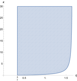
Figure 1: Domain ${\mathcal{D}}$ of the $(\eta,\hat{\kappa})$ theory parameters where non-asymptotically flat BHs, with the asymptotics Eqs. (81)–(84), can be constructed by choosing an appropriate value of the horizon-shooting parameter ${\bar{\pi}}_{0}$.

The projection of the domain ${\mathcal{D}}$ on the $\eta$ axis starts at $\eta=\frac{1}{3}$ and then extends to larger values of $\eta$, though it seems that when $\eta\gtrsim 1.65$ one needs very large values of $\hat{\kappa}\equiv\kappa r_{h}$ to find such solutions. When $\frac{1}{3}<\eta<1.654$, this region seems to extend indefinitely in the large-$\hat{\kappa}$ direction, i.e., to be defined by an inequality of the type $\hat{\kappa}>\hat{\kappa}_{\rm min}(\eta)$. [We recall that our numerical integrations use units where $r_{h}=1$, so that $\hat{\kappa}\equiv\kappa r_{h}$ is numerically equal to $\kappa$. However, one should keep in mind that torsion bigravity theories are parametrized by $\eta$ and $\kappa$ (with dimension of an inverse length), while the lower boundary of the domain ${\mathcal{D}}$ involves the dimensionless product $\hat{\kappa}\equiv\kappa r_{h}$.] From our numerical studies it seems that for $\frac{1}{3}<\eta\leq 0.6$ this region starts at $\hat{\kappa}=0$, i.e., that $\hat{\kappa}_{\rm min}(\eta)=0$. It is only for $\eta\gtrsim 0.7$ that we could not construct solutions for very small $\kappa$ so that $\hat{\kappa}_{\rm min}(\eta)>0$ . A sample of our approximate determination of the value of the lower boundary $\hat{\kappa}_{\rm min}(\eta)$ of the domain ${\mathcal{D}}$ is given in Table 1. Our present numerical investigations leave open the issue of whether the (fast-increasing) lower bound $\hat{\kappa}_{\rm min}(\eta)$ is finite for all values of $\eta$ or becomes infinite at some finite $\eta_{*}>1.654$.

Table 1: Sample of approximate values of the lower boundary $\hat{\kappa}_{\rm min}(\eta)$ of the domain of existence ${\mathcal{D}}$ of non-asymptotically flat BHs in the $(\eta,\hat{\kappa})$ plane.

$\eta$	$\hat{\kappa}_{\rm min}(\eta)$
$\frac{1}{3}<\eta\leq 0.6$	0
$0.7$	$0.05$
$1$	$0.34$
$1.3$	$1.25$
$1.6$	$9$
$1.642$	$30$
$1.654$	$120$

Let us also emphasize that, while we found above that linearized perturbations of the Schwarzschild  solution can only exist for all values of $r$ if $\hat{\kappa}$ is larger than the lower bound (67), this lower bound does not apply to nonlinear solutions. Indeed, the curve $\hat{\kappa}=(\eta(1+\eta))^{1/4}$ passes in the middle of the domain ${\mathcal{D}}$ and does not constitute an obstacle to the existence of nonlinear BH solutions.

Given (when $(\eta,\hat{\kappa})\in{\mathcal{D}}$) such a solution of the three ODEs (VII.2), one can then compute (using Eqs. (IV)) the other variables $V(r)$ and $F(r)=\Phi^{\prime}(r)$. The quadrature Eq. (13) yields also the radial evolution of $\Phi(r)$, and therefore the knowledge of $-g_{00}=\exp[2\Phi]$. Then one can also compute the radial evolution of the two independent contorsion components $K_{100}\equiv{K^{\hat{1}}}_{\hat{0}\hat{0}}$ and $K_{122}\equiv{K^{\hat{1}}}_{\hat{2}\hat{2}}$ using Eqs. (III). It is then easily found that both $K_{100}$ and $K_{122}$ grow exponentially $\sim\exp[+c\,r]$ (with the same constant $c$ entering $\tilde{l}$, Eq. (82)) at large radii.

Seen from a conventional Einsteinian perspective (see section 5 of Ref.Hayashi:1979wj ), one can consider that the contorsion tensor ${\bf K}$ (together with its covariant derivative, entering the rewriting of $F_{ij}$ in terms of ${\bf g}$ and ${\bf K}$) defines an effective stress-energy tensor ${\bf T}_{\rm eff}$ for the Einstein tensor of ${\bf g}$: ${\bf G}\equiv{\bf Ricci(g)}-\frac{1}{2}{\bf g}$. The metric of the vacuum solutions considered here can then be considered as being jointly generated by the “mass” $\frac{1}{2}r_{h}$ of the BH, together with the torsion field ${\bf K}$. From this point of view, it is the particular effective equation of state of the torsion-generated ${\bf T}_{\rm eff}\sim{\bf K}^{2}+{\bf\nabla K}+({\bf\nabla K})^{2}$ which allows an exponentially growing ${\bf K}\sim\exp[+c\,r]$ (when measured in a frame) to generate exponentially decaying metric tensor components ${\bf g}\sim\exp[-2c\,r]$ (in Schwarzschild  ​​-type coordinates). Let us finally note that the spatial geometry defined by $dl^{2}=g_{rr}dr^{2}+r^{2}\left(d\theta^{2}+\sin^{2}\theta\,d\phi^{2}\right)$, with $g_{rr}=L^{2}=\tilde{l}^{2}/(1-1/r)$ is rather unusual: though “the sphere at infinity” ($r\to+\infty$) has an infinite surface $4\pi r^{2}$, it is located at a finite radial distance, $\int_{1}^{+\infty}drL<\infty$, from the central BH.

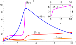
Figure 2: The metric fields, $-g_{00}$ (blue online), and $g_{rr}^{-1}$ (magenta on line), and the adimensionalized torsion fields, $r_{h}K_{100}$ (orange online), and $r_{h}K_{122}$ (red online), of a member of the two-parameter family of non-asymptotically-flat torsion-hairy BHs are displayed for the case $\eta=1$, $\hat{\kappa}=0.5$ and ${\bar{\pi}}_{0}=0$. The inset displays $\ln[g_{rr}^{-1}]$ to show the asymptotic exponential decay of $g_{rr}$.

We illustrate in Fig. 2 the metric and torsion structure of these solutions for the case $\eta=1$, $\hat{\kappa}=\frac{1}{2}$, and for the horizon parameter ${\bar{\pi}}_{0}=0$. [Note that $\hat{\kappa}=\frac{1}{2}>\hat{\kappa}_{\rm min}(1)\simeq 0.34$, and that the linearized bound (67) is significantly violated by the values $\eta=1$, $\hat{\kappa}=\frac{1}{2}$.] This Figure displays the four dimensionless functions $-g_{00}$, $g_{rr}^{-1}$, $r_{h}K_{100}$ and $r_{h}K_{122}$ versus $r/r_{h}$ (using units where $r_{h}=1$). Regularity at the horizon implies that, near $r=r_{h}$, $-g_{00}\sim g_{rr}^{-1}\sim r-r_{h}$, while $K_{100}\sim K_{122}\sim\sqrt{r-r_{h}}$. The asymptotic behavior at large $r$ of the metric coefficients is $-g_{00}\sim g_{rr}\sim\exp[-2\,cr]$, with $c\approx 0.05367$. That of the contorsion components is $K_{100}\sim K_{122}\sim\exp[+cr]$. The inset shows that the asymptotic exponential decay of $g_{rr}$ (corresponding to a linear slope for $\ln[g_{rr}^{-1}]\sim+2c\,r$) starts only for $r\gtrsim 8$.

X Asymptotically flat torsion-hairy BHs in the limit $\hat{\kappa}=\kappa r_{h}\to 0$

Though the results of the last two sections would tend to indicate that there do not exist asymptotically-flat BHs endowed with torsion hair, we actually discovered that the limiting sector of the $(\eta,\kappa)$ theory space where $\kappa\to 0$ does allow for the existence of a two-parameter family of torsion-hairy asymptotically-flat BHs.

Let us first recall that the limit $\kappa\to 0$ is of direct physical interest (and was actually the motivation of Refs. Nair:2008yh ; Nikiforova:2009qr for studying generalized Einstein-Cartan theories). Indeed the limit $\kappa\to 0$ physically corresponds to the hope that a value of $\kappa$ of cosmological scale, i.e., $\kappa\sim H_{0}$ where $H_{0}\sim 10^{-28}{\rm cm}^{-1}$ (leading to $\kappa r_{h}\sim 10^{-22}$ for a 3 $M_{\odot}$ BH) might define an interesting infrared modification of Einsteinian gravity. This hope was recently rekindled by the discovery Nikiforova:2020fbz that the formal $\kappa\to 0$ limit of torsion bigravity leads to well-defined field equations that can be perturbatively solved to all orders without encountering the usual small denominators $\sim\kappa^{-2}$ that enter both ghostfree massive gravity theories deRham:2010kj and their bimetric gravity generalizations Hassan:2011zd .

Taking the limit $\kappa\to 0$ in our system of ODEs, Eqs. (IV) or, equivalently, Eqs. (VII.2), leads to a well-defined system of three ODEs which admits horizon-regular solutions satisfying the usual boundary conditions (say, when using the formulation (VII.2), the regularity of the three variables $\tilde{l}(r),\tilde{w}(r),{\bar{\pi}}(r)$ at $r=r_{h}$).

One can again parametrize general local, horizon-regular solutions by varying the sole parameter ${\bar{\pi}}_{0}$, submitted to the constraint of leading to a positive $\tilde{l}_{0}^{2}$, Eq. (47). Here, it is important to use as shooting parameter ${\bar{\pi}}_{0}$ rather than $\tilde{\pi}_{0}\equiv{\bar{\pi}}_{0}/{\bar{\pi}}_{S}(r_{h})$, because ${\bar{\pi}}_{S}(r_{h})=-3/(\kappa r_{h})^{2}$ so that the horizon parameter $\tilde{\pi}_{0}^{S}=1$, leading to a Schwarzschild  BH, corresponds to ${\bar{\pi}}_{0}^{S}=-3/(\kappa r_{h})^{2}$. In other words, in the formal $\kappa\to 0$ limit (or better $\hat{\kappa}\equiv\kappa r_{h}\to 0$) a Schwarzschild  solution is obtained by choosing a divergently large (negative) value of ${\bar{\pi}}_{0}$. By contrast, when working with the $\kappa\to 0$ limit of our equations, we explored all the finite values of ${\bar{\pi}}_{0}$ (with the constraint $\tilde{l}_{0}^{2}>0$).

Before describing the structure of the asymptotically-flat BH solutions existing in the $\kappa\to 0$ limit, let us further clarify the physical meaning of the latter formal limit. Let us note first that the large-$r$ behavior of the $\kappa=0$ reduction of the system (VII.2) is significantly different from the large-$r$ behavior of its general $\kappa\neq 0$ version. Indeed, it is easily seen on the explicit formulas giving Eqs. (VII.2) (see Appendix A) that all the powers of $\kappa^{2}$ come accompanied by a corresponding power of $r^{2}$. In other words, the system (VII.2) crucially features the length scale $\kappa^{-1}$ and changes character between the region $r\ll\kappa^{-1}$ and the region $r\gg\kappa^{-1}$. Taking first (as we do here) the limit $\kappa\to 0$, and then the limit $r\to\infty$, corresponds to studying the asymptotics of the theory at large astrophysical distances from a BH ($r_{\rm astro}\gg r_{h}$) when considering, say, a cosmological-scale value $\kappa\sim H_{0}$ (with $r_{\rm astro}\ll\kappa^{-1}\sim H_{0}^{-1}$) . [Such a limit is often considered when studying solutions in massive gravity and bimetric gravity.] This shows that the BH solutions we are now discussing could be of potential astrophysical relevance.

Similarly to what happened for the non-asymptotically-flat BH solutions discussed in Section IX, the existence (when $\hat{\kappa}=0$) of a continuous family of asymptotically-flat BH solutions is linked with the existence of stable attractors in the $r\to+\infty$ limit of the first-order system (VII.2) (reduced by taking $\hat{\kappa}=0$). The $r\to+\infty$ asymptotics of the latter system leads again to a Fuchsian-type system, of the same form as in Section IX, say (denoting again $\rho\equiv\ln r$)

$$r\frac{d}{dr}{\bf X}\equiv\frac{d}{d\rho}{\bf X}={\bf V}({\bf X})\,,$$ (87)

but with the important difference that now

$${\bf X}=(\tilde{l},\tilde{w},{\bar{\pi}})\,,$$ (88)

is a three-dimensional vector, and ${\bf V}({\bf X})$ is a three-component vector function of ${\bf X}$. The three-component vector function ${\bf V}({\bf X})$ is drastically different from the two-component vector function ${\bf v}({\bf x})$ that entered Eq. (85), which was obtained by first setting $\tilde{l}=0$ and then considering the $r\to+\infty$ limit of the $\kappa\neq 0$ system (VII.2).

As before, the asymptotic system (87) describes a time-independent flow, with time variable $\rho\equiv\ln r\to+\infty$, and velocity field ${\bf V}({\bf X})$. This flow now takes place in the three-dimensional space of ${\bf X}=(\tilde{l},\tilde{w},{\bar{\pi}})$. We studied the fixed points of this flow (i.e., the values of ${\bf X}$ where ${\bf V}({\bf X})$ vanishes), and the attractive or repulsive nature of these fixed points when $\rho\to+\infty$ (as determined by studying the Jacobian matrix $\partial{\bf V}({\bf X})/\partial{\bf X}$ at these fixed points). We will leave to a future publication VN2020b a detailed analysis of all the fixed points of the flow ${\bf V}({\bf X})$, and of their nature.

For the time being, let us only mention that, among several attractive fixed points, we found a unique one that leads to an asymptotically flat geometrical structure. In terms of the “position vector” ${\bf X}=(\tilde{l},\tilde{w},{\bar{\pi}})$ this stable fixed point (at $\rho=+\infty$) of the flow (87) is given by

$${\bf X}_{\infty}=\left(\tilde{l}_{\infty},\tilde{w}_{\infty},{\bar{\pi}}_{\infty}\right)=\left(1,-1,+\frac{6}{\eta+1}\right).$$ (89)

The value $\tilde{l}_{\infty}=1$ corresponds to $(g_{rr})_{\infty}=L^{2}_{\infty}=1$, i.e., it corresponds to an asymptotically flat spatial metric. By taking into account the way the vector ${\bf X}(\rho)$ approaches its limit ${\bf X}_{\infty}$ as $\rho\to+\infty$, we could prove (using Eqs. (IV)) that $F(r)=\Phi^{\prime}(r)=O(r^{-3/2})$ at large $r$, so that the temporal metric $-g_{00}(r)=\exp(2\Phi)$ tends to a constant as $r\to\infty$. The value of the constant $-(g_{00})_{\infty}=\exp(2\Phi_{\infty})$ can be normalized to unity by appropriately rescaling $t$ (i.e., by a posteriori choosing an adequate value of the arbitrary integration constant arising in the quadrature $\Phi(r)=\int drF(r)+{\rm cst.}$). One also find that (using Eqs. (III)) the frame components $K_{100}$ and $K_{122}$ of the contorsion both decay in a power-law fashion as $r\to\infty$ (with some additional oscillatory behavior that will be discussed in Ref. VN2020b ). More precisely, $K_{100}=O(\frac{1}{r^{3/2}})$, while $K_{122}=O(\frac{1}{r})$ . As already mentioned, the fact that these solutions are stable attractors of our system of ODEs means that, for a given value of $\eta$, and after having scaled $r_{h}$ to one, we can construct a one-parameter family of torsion-hairy BHs by varying the horizon shooting parameter ${\bar{\pi}}_{0}$. For instance, in the case where $\eta=0.01$ we found that we can vary ${\bar{\pi}}_{0}$ between $-29$ and $+5$, and so generate a continuous family of asymptotically flat BH solutions. When varying ${\bar{\pi}}_{0}$ the values of the torsion fields correspondingly vary by large amounts.

One specific member of this one-parameter family of BH solutions (corresponding to the choice ${\bar{\pi}}_{0}=-5$) is displayed in Fig. 3. This Figure displays the four dimensionless functions $-g_{00}$, $g_{rr}^{-1}$, $r_{h}K_{100}$ and $r_{h}K_{122}$ versus $r/r_{h}$ (using units where $r_{h}=1$). Regularity at the horizon implies that all those functions vanish there (either linearly or in a square-root manner). Note that (because of our choice of a, phenomenologically required Damour:2019oru , small value for $\eta$) the metric functions are close to the Schwarzschild  one, $-g_{00}^{S}=[g_{rr}^{S}]^{-1}=1-r_{h}/r$, which is indicated as an hyphenated curve for comparison. At large radii both $g_{rr}(r)$ and $-g_{00}(r)$ (which we have appropriately rescaled) tend to 1, while $K_{100}$ and $K_{122}$ both decay in a power-law fashion: $K_{100}=O(\frac{1}{r^{3/2}})$, and $K_{122}=O(\frac{1}{r})$. The torsion fields constitute the torsion hair of the BH and show an interesting geometric deviation of order unity from an Einsteinian geometric structure.

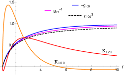
Figure 3: The metric fields, $-g_{00}$ (upper right curve, blue online), and $g_{rr}^{-1}$ (intermediate upper right curve, magenta on line), and the adimensionalized torsion fields, $r_{h}K_{100}$ (orange online), and $r_{h}K_{122}$ (red online), of a member of the two-parameter family of asymptotically-flat torsion-hairy BHs that exist in the $\kappa\to 0$ limit are illustrated for the case $\eta=0.01$ and ${\bar{\pi}}_{0}=-5$. While the metric structure of this BH is close to the Schwarzschild  one (hyphenated curve), its torsion structure exhibits a deviation of order unity from a purely Einsteinian structure.

XI Conclusions

We studied static, spherically-symmetric black hole (BH) solutions in torsion bigravity theories. These Einstein-Cartan-type theories (with propagating torsion) contain only two excitations: an Einsteinlike massless spin-2 one, and a massive spin-2 one. The parameter space for the vacuum solutions of torsion bigravity comprises the inverse range $\kappa$ of the massive spin-2 excitation, and the dimensionless ratio $\eta$ between the coupling of the massive spin-2 field and the coupling of the massless one.

We found three broad classes of BH solutions. First, the Schwarzschild  solution is an exact solution of torsion bigravity that exists all over the parameter space, but has zero torsion hair. We proved that one cannot deform a Schwarzschild  solution, at the linearized level, by adding an infinitesimal torsion hair.

Second, when considering finite values of the range, we found that in a large domain of parameter space (illustrated in Fig. 1) there exist BH solutions endowed with a torsion structure, but which are not asymptotically flat. The geometrical structure of these torsion-hairy, but non-asymptotically flat, BHs is illustrated in Fig. 2.

Finally, and most interestingly, we found that, in the limit of infinite range, there exist (for all values of the remaining theory parameter $\eta$) asymptotically flat BHs endowed with a (one-parameter-family) torsion structure. The geometrical structure of these asymptotically flat torsion-hairy BHs is illustrated in Fig. 3.

The latter BH solutions give an interesting example of non-Einsteinian (but still purely geometric) BH structures. They might be astrophysically meaningful if we consider the case where $\kappa$ is of the order of the Hubble constant. [In that case, as the range $\kappa^{-1}$ is very large but not infinite, the torsion-hairy BHs we constructed start mathematically deviating from flatness at radii $\sim\kappa^{-1}$. One should then embed them in a cosmological solution to check their astrophysical relevance.] We leave to future work a detailed description of the geometrical and physical properties of the asymptotically flat torsion-hairy black holes that exist in the limit of infinite inverse range.

The motivation of our present line of work is that torsion bigravity might define a theoretically healthy alternative to General Relativity that could lead to an interesting modified phenomenology for the physics of neutron stars, black holes and gravitational waves. Our past work has given some evidence that torsion bigravity has interesting theoretical features: notably the same number of degrees of freedom for spherically-symmetric solutions than ghost-free bimetric gravity Damour:2019oru , and the absence of any Vainshtein radius when considering the large-range limit $\kappa^{-1}\to\infty$ Nikiforova:2020fbz . We leave to future work a study of neutron-star solutions in the large-range limit, as well as a study of the dynamical stability of the BH solutions we have discussed in the present work.

Appendix A Explicit form of the field equations of static, spherically-symmetric torsion bigravity

The right-hand sides of the solutions (IV) of the two algebraic equations (IV) read

$$F^{\rm sol}(L,W,{\bar{\pi}})=\left\{\,3+2r\eta L[-6+(1+\eta){\bar{\pi}}]W\right.$$

$$\qquad+L^{2}[\,2\eta(1+\eta){\bar{\pi}}+\kappa^{2}r^{2}\eta(1+\eta){\bar{\pi}}^{2}$$

$$\qquad\left.-3(1+\eta+3r^{2}\eta W^{2})\,]\right\}/$$

$$\qquad\left\{\,2r[\,r\eta LW(3+(1+\eta){\bar{\pi}})-3\,]\,\right\}\;,$$

$$V^{\rm sol}(L,W,{\bar{\pi}})=\left\{9[(1+\eta){\bar{\pi}}-3]+6rLW[(1+\eta){\bar{\pi}}-6]\right.$$

$$\qquad+L^{2}(\,3+(1+\eta){\bar{\pi}}\,)[\,-3(1+\eta)+\kappa^{2}r^{2}\eta{\bar{\pi}}^{2}(1+\eta)$$

$$\qquad+3r^{2}\eta W^{2}\left.-2\eta{\bar{\pi}}(1+\eta)(r^{2}W^{2}-1)\,]\right\}/$$

$$\qquad\left\{2rL[3+(1+\eta){\bar{\pi}}](r\eta LW[3+(1+\eta){\bar{\pi}}]-3)\right\}.$$ (90)

The explicit forms of the right-hand sides of our reduced system of three ODEs (IV) read

$$D{\bar{\pi}}(L,W,{\bar{\pi}}) = \frac{3+3rLW+(1+\eta){\bar{\pi}}(rLW-2)}{r(1+\eta)}\;,$$

$$DL(L,W,{\bar{\pi}}) = \frac{N_{DL}}{D_{DL}}\;,$$

$$DW(L,W,{\bar{\pi}}) = \frac{N_{DW}}{D_{DW}}\;,$$ (91)

where

$$N_{DL}= L\left\{9[9-27\eta+12\eta(1+\eta){\bar{\pi}}+\eta(1+\eta)^{2}{\bar{\pi}}^{2}]+6r\eta LW[81(\eta-1)-18\eta(1+\eta){\bar{\pi}}-12\eta(1+\eta)^{2}{\bar{\pi}}^{2}+\eta(1+\eta)^{3}{\bar{\pi}}^{3}]\right.$$

$$-2r\eta(3+(1+\eta){\bar{\pi}})L^{3}W[\,\kappa^{2}r^{2}\eta(1+\eta)^{2}(2\eta-1){\bar{\pi}}^{3}+3\eta(1+\eta)^{2}{\bar{\pi}}^{2}(\kappa^{2}r^{2}+2\eta-2r^{2}\eta W^{2})$$

$$+27(-(1+\eta)^{2}+r^{2}(\eta-1)\eta W^{2})-9\eta(1+\eta){\bar{\pi}}(-1+\kappa^{2}r^{2}-\eta+r^{2}(1+\eta)W^{2})\,]$$

$$+3L^{2}[\,2\eta(1+\eta)^{2}(\eta(1+\eta)+\kappa^{2}r^{2}(2\eta-1)){\bar{\pi}}^{3}+\kappa^{2}r^{2}\eta^{2}(1+\eta)^{3}{\bar{\pi}}^{4}-18r^{2}\eta(1+\eta){\bar{\pi}}(\kappa^{2}-(\eta-1)W^{2})$$

$$\left.-3\eta(1+\eta)^{2}{\bar{\pi}}^{2}(1+\kappa^{2}r^{2}-3\eta+11r^{2}\eta W^{2})+27(-(1+\eta)^{2}+r^{2}\eta(1+13\eta)W^{2})\,]\right\}\;,$$

$$D_{DL}= 6r(1+\eta)(\eta(1+\eta){\bar{\pi}}^{2}-9)[r\eta LW(3+(1+\eta){\bar{\pi}})-3]\;,$$

$$N_{DW}= \kappa^{2}r^{3}\eta^{2}(1+\eta)^{4}L^{3}{\bar{\pi}}^{5}W-9(1+\eta)^{2}{\bar{\pi}}^{2}[2-11r\eta LW+r\eta L^{3}W(1+3\kappa^{2}r^{2}-3\eta+3r^{2}\eta W^{2})$$

$$-2L^{2}(1+2\kappa^{2}r^{2}-\eta+6r^{2}\eta W^{2})]+81[4+3r(1-3\eta)LW+2r^{2}(-5+\eta)\eta L^{2}W^{2}$$

$$+rL^{3}W(-(1+\eta)^{2}+r^{2}(-3+\eta)\eta W^{2})]+27(1+\eta){\bar{\pi}}[-4+r(-3+\eta)LW$$

$$+rL^{3}W(-1-2(1+\kappa^{2}r^{2})\eta-\eta^{2}+r^{2}(-3+\eta)\eta W^{2})+2L^{2}(1+\kappa^{2}r^{2}+\eta+2r^{2}\eta^{2}W^{2})]$$

$$-r\eta(1+\eta)^{3}L^{2}{\bar{\pi}}^{4}[2r(3\kappa^{2}+\eta(1+\eta)W^{2})+LW(\kappa^{2}r^{2}(2-7\eta)-2\eta(1+\eta)+2r^{2}\eta(1+\eta)W^{2})]$$

$$+3(1+\eta)^{2}L{\bar{\pi}}^{3}[r\eta(1+\eta)W-r\eta L^{2}W(1-3\kappa^{2}r^{2}(-1+\eta)-4\eta-5\eta^{2}+5r^{2}\eta(1+\eta)W^{2})$$

$$-2L(2\eta(1+\eta)+\kappa^{2}r^{2}(-1+2\eta)+r^{2}\eta(-1+\eta+2\eta^{2})W^{2})]\;,$$

$$D_{DW}= 2r^{2}(1+\eta)L(3+(1+\eta){\bar{\pi}})(-9+\eta(1+\eta){\bar{\pi}}^{2})[-3+r\eta L(3+(1+\eta){\bar{\pi}})W]\;.$$ (92)

When rescaling the variables $L$ and $W$ by their Schwarzschild  values, the latter system becomes the first-order system (VII.2) for the radial evolution of $\tilde{l}\equiv L/L_{S}$, $\tilde{w}\equiv W/W_{S}$ and ${\bar{\pi}}$. The right-hand sides of Eqs. (VII.2) read (when using $r_{h}=1$)

$$D{\bar{\pi}}(\tilde{l},\tilde{w},{\bar{\pi}}) = \frac{3-3\tilde{l}\tilde{w}-(1+\eta){\bar{\pi}}(2+\tilde{l}\tilde{w})}{r(1+\eta)}\;,$$

$$D\tilde{l}(\tilde{l},\tilde{w},{\bar{\pi}}) = \frac{N_{\tilde{l}}}{D_{\tilde{l}}}\;,$$

$$D\tilde{w}(\tilde{l},\tilde{w},{\bar{\pi}}) = \frac{N_{\tilde{w}}}{D_{\tilde{w}}}\;,$$ (93)

where

$$N_{\tilde{l}}= \tilde{l}\left\{9[\,9(r+4\eta-3r\eta)+12(r-1)\eta(1+\eta){\bar{\pi}}+(r-2)\eta(1+\eta)^{2}{\bar{\pi}}^{2}\,]-3\eta\tilde{l}[\,27(5+6r(\eta-1)-7\eta)\right.$$

$$-9(1+\eta)(1+(-3+4r)\eta){\bar{\pi}}-3(-9+8r)\eta(1+\eta)^{2}{\bar{\pi}}^{2}+(-1+2r)\eta(1+\eta)^{3}{\bar{\pi}}^{3}\,]\tilde{w}$$

$$+2\eta\tilde{l}^{\,3}(3+(1+\eta){\bar{\pi}})\tilde{w}[\,\kappa^{2}r^{3}\eta(1+\eta)^{2}(-1+2\eta){\bar{\pi}}^{3}+3\eta(1+\eta)^{2}{\bar{\pi}}^{2}(\kappa^{2}r^{3}+2r\eta-2(r-1)\eta\tilde{w}^{2})$$

$$+27(-r(1+\eta)^{2}+(r-1)(\eta-1)\eta\tilde{w}^{2})-9\eta(1+\eta){\bar{\pi}}(r(-1+\kappa^{2}r^{2}-\eta)+(r-1)(1+\eta)\tilde{w}^{2})\,]$$

$$+3\tilde{l}^{\,2}[\,2r\eta(1+\eta)^{2}(\eta(1+\eta)+\kappa^{2}r^{2}(-1+2\eta)){\bar{\pi}}^{3}+\kappa^{2}r^{3}\eta^{2}(1+\eta)^{3}{\bar{\pi}}^{4}$$

$$+18\eta(1+\eta){\bar{\pi}}(-\kappa^{2}r^{3}+(r-1)(\eta-1)\tilde{w}^{2})-3\eta(1+\eta)^{2}{\bar{\pi}}^{2}(r+\kappa^{2}r^{3}-3r\eta+11(r-1)\eta\tilde{w}^{2})$$

$$\left.+27(-r(1+\eta)^{2}+(r-1)\eta(1+13\eta)\tilde{w}^{2})\,]{\color[rgb]{1,1,1}\tilde{l}}\right\}\;,$$

$$D_{\tilde{l}}= 6(1-r)r(1+\eta)(-9+\eta(1+\eta){\bar{\pi}}^{2})[3+\eta\tilde{l}(3+(1+\eta){\bar{\pi}})\tilde{w}]\;,$$

$$N_{\tilde{w}}= \kappa^{2}r^{3}\eta^{2}(1+\eta)^{4}\tilde{l}^{\,3}{\bar{\pi}}^{5}\tilde{w}-9(1+\eta)^{2}{\bar{\pi}}^{2}[\,2-2r+(8-9r)\eta\tilde{l}\tilde{w}+\eta\tilde{l}^{\,3}\tilde{w}(r+3\kappa^{2}r^{3}-3r\eta+3(-1+r)\eta\tilde{w}^{2})$$

$$+\tilde{l}^{\,2}(2r(1+2\kappa^{2}r^{2}-\eta)+(-9+10r)\eta\tilde{w}^{2})\,]+81[\,4-4r+(-6+5r+6\eta-7r\eta)\tilde{l}\tilde{w}-\eta(13-12r+\eta)\tilde{l}^{\,2}\tilde{w}^{2}$$

$$+\tilde{l}^{\,3}\tilde{w}(-r(1+\eta)^{2}+(-1+r)(-3+\eta)\eta\tilde{w}^{2})\,]+\eta(1+\eta)^{3}\tilde{l}^{\,2}{\bar{\pi}}^{4}\left\{6\kappa^{2}r^{3}+\eta(1+\eta)\tilde{w}^{2}+\tilde{l}\tilde{w}[\,r(2\eta(1+\eta)\right.$$

$$\left.+\kappa^{2}r^{2}(-2+7\eta))-2(-1+r)\eta(1+\eta)\tilde{w}^{2}\,]{\color[rgb]{1,1,1}\tilde{l}}\right\}+3(1+\eta)^{2}\tilde{l}{\bar{\pi}}^{3}\left\{{\color[rgb]{1,1,1}\tilde{l}}-(-2+r)\eta(1+\eta)\tilde{w}\right.$$

$$+\eta\tilde{l}^{\,2}\tilde{w}(r(-1+3\kappa^{2}r^{2}(-1+\eta)+4\eta+5\eta^{2})-5(-1+r)\eta(1+\eta)\tilde{w}^{2})+2\tilde{l}[\,r(2\eta(1+\eta)+\kappa^{2}r^{2}(-1+2\eta))$$

$$\left.-(-1+r-\eta)\eta(1+\eta)\tilde{w}^{2}\,]{\color[rgb]{1,1,1}\tilde{l}}\right\}-27(1+\eta){\bar{\pi}}[\,4-4r+(r+4\eta-3r\eta)\tilde{l}\tilde{w}+\tilde{l}^{\,3}\tilde{w}(r(1+2\eta+2\kappa^{2}r^{2}\eta+\eta^{2})$$

$$-(-1+r)(-3+\eta)\eta\tilde{w}^{2})+2\tilde{l}^{\,2}(r(1+\kappa^{2}r^{2}+\eta)+\eta(3-2r+\eta)\tilde{w}^{2})\,]\;,$$

$$D_{\tilde{w}}= 2(1-r)r(1+\eta)\tilde{l}(3+(1+\eta){\bar{\pi}})(-9+\eta(1+\eta){\bar{\pi}}^{2})[\,3+\eta\tilde{l}(3+(1+\eta){\bar{\pi}})\tilde{w}\,]\;.$$ (94)

References

- (1) B. Abbott et al. [LIGO Scientific and Virgo], “GWTC-1: A Gravitational-Wave Transient Catalog of Compact Binary Mergers Observed by LIGO and Virgo during the First and Second Observing Runs,” Phys. Rev. X 9, no.3, 031040 (2019) [arXiv:1811.12907 [astro-ph.HE]].
- (2) K. Akiyama et al. [Event Horizon Telescope], “First M87 Event Horizon Telescope Results. I. The Shadow of the Supermassive Black Hole,” Astrophys. J. 875, no.1, L1 (2019) [arXiv:1906.11238 [astro-ph.GA]].
- (3) B. Abbott et al. [LIGO Scientific and Virgo], “Tests of General Relativity with the Binary Black Hole Signals from the LIGO-Virgo Catalog GWTC-1,” Phys. Rev. D 100, no.10, 104036 (2019) [arXiv:1903.04467 [gr-qc]].
- (4) W. Israel, “Event horizons in static vacuum space-times,” Phys. Rev. 164, 1776-1779 (1967)
- (5) B. Carter, “Axisymmetric Black Hole Has Only Two Degrees of Freedom,” Phys. Rev. Lett. 26, 331-333 (1971)
- (6) D. Robinson, “Uniqueness of the Kerr black hole,” Phys. Rev. Lett. 34, 905-906 (1975)
- (7) J. Bekenstein, “Novel ÔÔno-scalar-hairÕÕ theorem for black holes,” Phys. Rev. D 51, no.12, 6608 (1995)
- (8) J. D. Bekenstein, “Nonexistence of baryon number for static black holes,” Phys. Rev. D 5, 1239-1246 (1972)
- (9) J. Bekenstein, “Nonexistence of baryon number for black holes. ii,” Phys. Rev. D 5, 2403-2412 (1972)
- (10) C. M. Will, “The Confrontation between General Relativity and Experiment,” Living Rev. Rel. 17, 4 (2014) [arXiv:1403.7377 [gr-qc]].
- (11) S. Capozziello and M. De Laurentis, “Extended Theories of Gravity,” Phys. Rept. 509, 167 (2011) [arXiv:1108.6266 [gr-qc]].
- (12) E. Berti et al., “Testing General Relativity with Present and Future Astrophysical Observations,” Class. Quant. Grav. 32, 243001 (2015)
- (13) T. P. Sotiriou and S. Y. Zhou, “Black hole hair in generalized scalar-tensor gravity,” Phys. Rev. Lett. 112, 251102 (2014) [arXiv:1312.3622 [gr-qc]].
- (14) T. P. Sotiriou and S. Y. Zhou, “Black hole hair in generalized scalar-tensor gravity: An explicit example,” Phys. Rev. D 90, 124063 (2014) [arXiv:1408.1698 [gr-qc]].
- (15) D. D. Doneva and S. S. Yazadjiev, “New Gauss-Bonnet Black Holes with Curvature-Induced Scalarization in Extended Scalar-Tensor Theories,” Phys. Rev. Lett. 120, no.13, 131103 (2018) [arXiv:1711.01187 [gr-qc]].
- (16) H. O. Silva, J. Sakstein, L. Gualtieri, T. P. Sotiriou and E. Berti, “Spontaneous scalarization of black holes and compact stars from a Gauss-Bonnet coupling,” Phys. Rev. Lett. 120, no.13, 131104 (2018) [arXiv:1711.02080 [gr-qc]].
- (17) C. de Rham, G. Gabadadze and A. J. Tolley, “Resummation of Massive Gravity,” Phys. Rev. Lett. 106, 231101 (2011) [arXiv:1011.1232 [hep-th]].
- (18) S. F. Hassan and R. A. Rosen, “Bimetric Gravity from Ghost-free Massive Gravity,” JHEP 1202, 126 (2012) [arXiv:1109.3515 [hep-th]].
- (19) M. S. Volkov, “Hairy black holes in the ghost-free bigravity theory,” Phys. Rev. D 85, 124043 (2012) [arXiv:1202.6682 [hep-th]].
- (20) R. Brito, V. Cardoso and P. Pani, “Black holes with massive graviton hair,” Phys. Rev. D 88, 064006 (2013) [arXiv:1309.0818 [gr-qc]].
- (21) E. Babichev and R. Brito, “Black holes in massive gravity,” Class. Quant. Grav. 32, 154001 (2015) [arXiv:1503.07529 [gr-qc]].
- (22) J. Enander and E. Mortsell, “On stars, galaxies and black holes in massive bigravity,” JCAP 11, 023 (2015) [arXiv:1507.00912 [astro-ph.CO]].
- (23) C. Deffayet and T. Jacobson, “On horizon structure of bimetric spacetimes,” Class. Quant. Grav. 29, 065009 (2012) [arXiv:1107.4978 [gr-qc]].
- (24) E. Babichev and A. Fabbri, “Instability of black holes in massive gravity,” Class. Quant. Grav. 30, 152001 (2013) [arXiv:1304.5992 [gr-qc]].
- (25) R. Brito, V. Cardoso and P. Pani, “Massive spin-2 fields on black hole spacetimes: Instability of the Schwarzschild and Kerr solutions and bounds on the graviton mass,” Phys. Rev. D 88, no.2, 023514 (2013) [arXiv:1304.6725 [gr-qc]].
- (26) E. Cartan, “Sur les variétés à connexion affine et la théorie de la relativité généralisée. (première partie),” Annales Sci. Ecole Norm. Sup. 40, 325 (1923).
- (27) E. Cartan, “Sur les variétés à connexion affine et la théorie de la relativité généralisée. (Suite).,” Annales Sci. Ecole Norm. Sup. 41, 1 (1924).
- (28) E. Cartan, “Sur les variétés à connexion affine et la théorie de la relativité généralisée. (deuxième partie)),” Annales Sci. Ecole Norm. Sup. 42, 17 (1925).
- (29) H. Weyl, “A Remark on the coupling of gravitation and electron,” Phys. Rev. 77, 699-701 (1950)
- (30) D. W., Sciama, “On the analogy between charge and spin in general relativity”, in Recent Developments in General Relativity, (Pergamon Press, Oxford, 1962), pp. 415–439.
- (31) T. W. B. Kibble, “Lorentz invariance and the gravitational field,” J. Math. Phys. 2, 212 (1961).
- (32) F. W. Hehl, P. Von Der Heyde, G. D. Kerlick and J. M. Nester, “General Relativity with Spin and Torsion: Foundations and Prospects,” Rev. Mod. Phys. 48, 393 (1976).
- (33) P. Baekler and F. W. Hehl, “Beyond Einstein-Cartan gravity: Quadratic torsion and curvature invariants with even and odd parity including all boundary terms,” Class. Quant. Grav. 28, 215017 (2011) [arXiv:1105.3504 [gr-qc]].
- (34) E. Sezgin and P. van Nieuwenhuizen, “New Ghost Free Gravity Lagrangians with Propagating Torsion,” Phys. Rev. D 21, 3269 (1980).
- (35) E. Sezgin, “Class of Ghost Free Gravity Lagrangians With Massive or Massless Propagating Torsion,” Phys. Rev. D 24, 1677 (1981).
- (36) K. Hayashi and T. Shirafuji, “Gravity from Poincare Gauge Theory of the Fundamental Particles. 1. General Formulation,” Prog. Theor. Phys. 64, 866 (1980) Erratum: [Prog. Theor. Phys. 65, 2079 (1981)].
- (37) K. Hayashi and T. Shirafuji, “Gravity From Poincare Gauge Theory Of The Fundamental Particles. 2. Equations Of Motion For Test Bodies And Various Limits,” Prog. Theor. Phys. 64, 883 (1980) Erratum: [Prog. Theor. Phys. 65, 2079 (1981)].
- (38) K. Hayashi and T. Shirafuji, “Gravity From Poincare Gauge Theory of the Fundamental Particles. 3. Weak Field Approximation,” Prog. Theor. Phys. 64, 1435 (1980) Erratum: [Prog. Theor. Phys. 66, 741 (1981)].
- (39) K. Hayashi and T. Shirafuji, “Gravity From Poincare Gauge Theory of the Fundamental Particles. 4. Mass and Energy of Particle Spectrum,” Prog. Theor. Phys. 64, 2222 (1980).
- (40) V. P. Nair, S. Randjbar-Daemi and V. Rubakov, “Massive Spin-2 fields of Geometric Origin in Curved Spacetimes,” Phys. Rev. D 80, 104031 (2009) [arXiv:0811.3781 [hep-th]].
- (41) V. Nikiforova, S. Randjbar-Daemi and V. Rubakov, “Infrared Modified Gravity with Dynamical Torsion,” Phys. Rev. D 80, 124050 (2009) [arXiv:0905.3732 [hep-th]].
- (42) C. Deffayet and S. Randjbar-Daemi, “Non linear Fierz-Pauli theory from torsion and bigravity,” Phys. Rev. D 84, 044053 (2011) [arXiv:1103.2671 [hep-th]].
- (43) T. Damour and V. Nikiforova, “Spherically symmetric solutions in torsion bigravity,” Phys. Rev. D 100, no.2, 024065 (2019) [arXiv:1906.11859 [gr-qc]].
- (44) V. Nikiforova, S. Randjbar-Daemi and V. Rubakov, “Self-accelerating Universe in modified gravity with dynamical torsion,” Phys. Rev. D 95, no. 2, 024013 (2017) [arXiv:1606.02565 [hep-th]].
- (45) V. Nikiforova, “The stability of self-accelerating Universe in modified gravity with dynamical torsion,” Int. J. Mod. Phys. A 32, no. 23n24, 1750137 (2017) [arXiv:1705.00856 [hep-th]].
- (46) V. Nikiforova, “Stability of self-accelerating Universe in modified gravity with dynamical torsion: the case of small background torsion,” Int. J. Mod. Phys. A 33, no. 07, 1850039 (2018) [arXiv:1711.03718 [hep-th]].
- (47) V. Nikiforova and T. Damour, “Infrared modified gravity with propagating torsion: instability of torsionfull de Sitter-like solutions,” Phys. Rev. D 97, no. 12, 124014 (2018) [arXiv:1804.09215 [gr-qc]].
- (48) V. Nikiforova, “Absence of a Vainshtein radius in torsion bigravity,” Phys. Rev. D 101, no.6, 064017 (2020) [arXiv:2001.07148 [gr-qc]].
- (49) A. I. Vainshtein, “To the problem of nonvanishing gravitation mass,” Phys. Lett. 39B, 393 (1972).
- (50) D. G. Boulware and S. Deser, “Can gravitation have a finite range?,” Phys. Rev. D 6, 3368 (1972).
- (51) E. Babichev, C. Deffayet and R. Ziour, “The Vainshtein mechanism in the Decoupling Limit of massive gravity,” JHEP 0905, 098 (2009) [arXiv:0901.0393 [hep-th]].
- (52) V. Nikiforova, in preparation.
- (53) I. Buchbinder, D. Gitman, V. Krykhtin and V. Pershin, “Equations of motion for massive spin-2 field coupled to gravity,” Nucl. Phys. B 584, 615-640 (2000) [arXiv:hep-th/9910188 [hep-th]].