Extended stochastic block models
with application to criminal networks

Abstract

Reliably learning group structures among nodes in network data is challenging in several applications. We are particularly motivated by studying covert networks that encode relationships among criminals. These data are subject to measurement errors, and exhibit a complex combination of an unknown number of core-periphery, assortative and disassortative structures that may unveil key architectures of the criminal organization. The coexistence of these noisy block patterns limits the reliability of routinely-used community detection algorithms, and requires extensions of model-based solutions to realistically characterize the node partition process, incorporate information from node attributes, and provide improved strategies for estimation and uncertainty quantification. To cover these gaps, we develop a new class of extended stochastic block models (esbm) that infer groups of nodes having common connectivity patterns via Gibbs-type priors on the partition process. This choice encompasses many realistic priors for criminal networks, covering solutions with fixed, random and infinite number of possible groups, and facilitates the inclusion of node attributes in a principled manner. Among the new alternatives in our class, we focus on the Gnedin process as a realistic prior that allows the number of groups to be finite, random and subject to a reinforcement process coherent with criminal networks. A collapsed Gibbs sampler is proposed for the whole esbm class, and refined strategies for estimation, prediction, uncertainty quantification and model selection are outlined. The esbm performance is illustrated in realistic simulations and in an application to an Italian mafia network, where we unveil key complex block structures, mostly hidden from state-of-the-art alternatives.

13.3pt

,
and

1 Introduction

Network data are ubiquitous in modern applications, and there is recurring interest in block structures defined by groups of nodes that share similar connectivity patterns (e.g., Fortunato and Hric, 2016). Our focus is on studying networks of individuals involved in organizing crime. In this setting, it is of considerable interest to infer shared connectivity patterns among different suspects, based on data provided by investigations, in order to obtain key insights into the hierarchical structure of criminal organizations (e.g., Campana, 2016; Faust and Tita, 2019; Diviák, 2019; Campana and Varese, 2020).

The relevance of this endeavor has motivated an increasing shift in modern forensic studies away from classical descriptive analyses of criminal networks (e.g., Krebs, 2002; Carley, Lee and Krackhardt, 2002; Morselli, 2009; Malm and Bichler, 2011; Agreste et al., 2016; Grassi et al., 2019; Cavallaro et al., 2020), and towards studying more complex group structures involving the monitored suspects (e.g., Ferrara et al., 2014; Calderoni and Piccardi, 2014; Magalingam, Davis and Rao, 2015; Calderoni, Brunetto and Piccardi, 2017; Liu et al., 2018; Sangkaran, Abdullah and Jhanjhi, 2020). These contributions have provided valuable initial insights into the structure and functioning of several criminal organizations. However, the focus has been on classical community detection algorithms (Girvan and Newman, 2002; Newman and Girvan, 2004; Newman, 2006; Blondel et al., 2008), which infer groups of criminals characterized by dense within-block connectivity and sparser connections between different blocks (Fortunato and Hric, 2016). Such approaches are overly simplified and ignore other fundamental block structures, such as core-periphery, disassortative and weak community patterns (e.g., Fortunato and Hric, 2016). These more nuanced structures are inherent to criminal organizations, which exhibit an intricate combination of vertical and horizontal hierarchies of block interactions (Paoli, 2007; Morselli, Giguère and Petit, 2007; Le, 2012; Catino, 2014). Disentangling such complex architectures is fundamental to inform preventive and repressive operations. However, this task requires improved methods combined with more realistic representations of criminal networks that incorporate a broader set of recurring block structures, beyond assortative communities.

An initial strategy for addressing the above objectives is to consider spectral clustering algorithms (Von Luxburg, 2007) and stochastic block models (Holland, Laskey and Leinhardt, 1983; Nowicki and Snijders, 2001). Both methods learn more general block architectures in network data and hence, despite their limited use in forensic studies, are expected to unveil criminal structures currently hidden to community detection algorithms. Nonetheless, as clarified in Sections 1.1–1.2, several aspects of criminal network studies still require careful statistical innovations. A crucial one is the coexistence of several community, core-periphery and disassortative architectures whose number, size and structure are unknown and partially obscured by the measurement errors arising from the investigations. To ensure accurate learning in these challenging settings it is fundamental to rely on an extended, yet interpretable, class of model-based solutions encompassing a variety of flexible mechanisms for the formation of suspect groups. Such processes should also allow structured inclusion of external information and facilitate the adoption of principled methods for estimation, prediction, uncertainty quantification and model selection, within a single realistic modeling framework.

1.1 The Infinito network

Our motivation is drawn from a large law-enforcement operation, named Operazione Infinito, that was conducted in Italy from 2007 to 2009 for disentangling and disrupting the core structure of the ’Ndrangheta mafia in Lombardy, north of Italy. According to the pre-trial detention order produced by the preliminary investigation judge of Milan, such a criminal organization, also referred to as La Lombardia, is a key example of a deeply rooted, highly structured and hard to untangle covert architecture with a disruptive and pervasive impact, both locally and internationally (Paoli, 2007; Catino, 2014). This motivates our efforts to provide an improved understanding of its hidden hierarchical structures via innovative block-modeling of the relationships among its monitored affiliates.

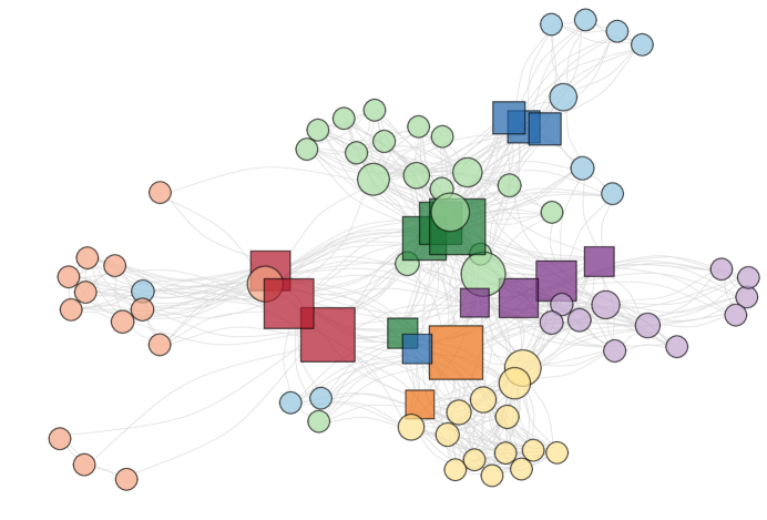
Figure 1: Graphical representation of the Infinito network. Node positions are obtained via force-directed placement (Fruchterman and Reingold, 1991). Node size is proportional to the corresponding betweenness, whereas colors indicate the presumed locale membership. Darker square nodes represent the bosses of each locale, while lighter circles indicate the affiliates.

Raw data are available at https://sites.google.com/site/ucinetsoftware/datasets/covert-networks and comprise information on the co-participation of 156 suspects at 47 monitored summits of the criminal organization, as reported in the judicial acts¹ that were issued upon request by the prosecution. Consistent with our main goal of shedding light on the internal structure of La Lombardia via inference on the block connectivity patterns among its affiliates, we focus on the reduced set of 118 suspects that attended at least one summit and were classified in the judicial acts as members of this specific criminal organization. Since only $18\%$ of these affiliate pairs co-attended at least one of the summits and, among them, just $5\%$ co-participated in more than one meeting, we consider here the binary adjacency matrix indicating the presence or absence of a co-attendance in at least one of the monitored summits. Due to the sparse and almost-binary form of the original counts, this dichotomization leads to a negligible loss of information and is beneficial in reducing the noise that may arise from investigations of multiple summits. Moreover, because of the highly regulated ’Ndrangheta coordinating processes (Paoli, 2007; Catino, 2014), the co-attendance of at least one summit is arguably sufficient to declare the presence of a connection among two affiliates.

More problematic is the possible presence of false negatives which may arise in such studies as a result of coverting strategies implemented by the criminal organization to carefully balance the tradeoff between efficiency and security (Morselli, Giguère and Petit, 2007). These covert patterns are not altered by the dichotomization procedure, and further motivate the development of improved methods for principled uncertainty quantification and structured borrowing of information among affiliates via the inclusion of available knowledge on the criminal organization and on suspects’ external attributes. For example, current forensic theories (e.g., Paoli, 2007; Catino, 2014) and initial quantitative analyses (e.g., Calderoni and Piccardi, 2014; Calderoni, Brunetto and Piccardi, 2017) suggest that the internal organization of ’Ndrangheta revolves around specific blood family relations, which may be further aggregated at the territorial level in structural coordinated units, named locali. Each locale controls a specific territory, and has a further layer of regulated hierarchy defined by a group of affiliates, and comparatively fewer bosses that are in charge of leading the locale, managing the funds, overseeing violent actions and guaranteeing the communication flows. Information on presumed locale membership and role can be retrieved, for each suspect of interest, from the judicial acts¹ of Operazione Infinito and, as shown in the graphical representation of the Infinito network in Figure 1, could help in assisting inference on the hidden underlying block structure, thus reducing the impact of coverting strategies.

The inclusion of the aforementioned node attributes motivates careful and principled probabilistic representations accounting for the fact that these sources of external information are produced by an investigation process and, therefore, may be prone to measurement errors. Despite its relevance and potential benefits, this endeavor has been largely neglected in the analysis of criminal networks and, as discussed in Section 1.2, state-of-the-art methods for block-modeling lack a general solution to include error-prone node attribute effects in the partition process and quantify the magnitude of the improvements relative to no supervision. To cover this gap and flexibly learn the complex variety of block structures in noisy criminal networks, we develop a novel class of extended stochastic block models (esbm) that formally quantify uncertainty in the suspects’ grouping structure — including in the number, size and composition of the blocks — via Gibbs-type priors (Gnedin and Pitman, 2005; Lijoi, Mena and Prünster, 2007a, b; Lijoi, Prünster and Walker, 2008) for the underlying partition; see also De Blasi et al. (2015) for a recent review.

As clarified in Section 2, although the block-modeling literature has focused on a much less extensive set of processes, the Gibbs-type class is well motivated in providing broad, interpretable and realistic probabilistic generative mechanisms for the formation of suspects’ groups. This allows careful incorporation of probabilistic structure within a single modeling framework which is amenable to novel extensions for the inclusion of probabilistic homophily with respect to error-prone external attributes, and for careful model-based inference on the partition structure via refined methods for estimation, uncertainty quantification, model selection and prediction. To assess out-of-sample predictive performance, we perform inference on the $V=84$ suspects affiliated to the $5$ most populated locali, and hold out as a test set the $34$ members of those smaller-sized locali with $\leq 6$ monitored affiliates. As discussed in Calderoni and Piccardi (2014), such a choice is also beneficial in reducing potential issues arising from the incomplete identification of low-sized locali during investigations, and, due to the modular organization of ’Ndrangheta (e.g., Paoli, 2007; Catino, 2014), it arguably leads to a more accurate learning of its core recurring hierarchies.

1.2 Relevant literature

The relevance of learning block structures in networks has motivated a collective effort by various disciplines towards the development of methods for detecting node groups, ranging from algorithmic strategies (Girvan and Newman, 2002; Newman and Girvan, 2004; Newman, 2006; Von Luxburg, 2007; Blondel et al., 2008) to model-based solutions (Holland, Laskey and Leinhardt, 1983; Nowicki and Snijders, 2001; Kemp et al., 2006; Airoldi et al., 2008; Karrer and Newman, 2011; Athreya et al., 2017; Geng, Bhattacharya and Pati, 2019); see Fortunato and Hric (2016), Abbe (2017), and Lee and Wilkinson (2019) for an overview.

Despite being routinely implemented in criminal network studies, most algorithmic approaches focus on detecting communities characterized by a dense connectivity within each block and sparser connections among different blocks (Girvan and Newman, 2002; Newman and Girvan, 2004; Newman, 2006; Blondel et al., 2008). This constrained search is expected to provide a limited and possibly biased view of the key modules that are hidden in criminal networks. For instance, Figure 1 clearly highlights a core-periphery structure underlying the Infinito network, with communities of affiliates in peripheral positions and groups of bosses at the core. According to panel (a) in Figure 2, state-of-the-art algorithms for community detection (Blondel et al., 2008) applied to the Infinito network obscure such patterns by over-collapsing some locali, while failing to separate affiliates from bosses.

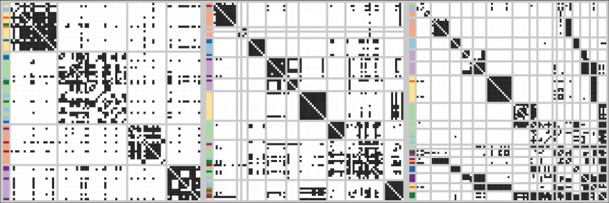
Figure 2: Adjacency matrix of the Infinito network with nodes re-ordered and partitioned in blocks according to the clustering structure estimated under three different methods: (a) community detection via the Louvain algorithm (Blondel et al., 2008); (b) spectral clustering (Von Luxburg, 2007) with the number of groups obtained via a combination of the model selection procedures in the R package randnet; (c) esbm with supervised Gnedin process prior. Black and white cells represent edges and non-edges, respectively. Side colors correspond to the different locali, with darker and lighter shades denoting bosses and affiliates, respectively.

These issues motivate focus on alternative solutions aimed at grouping nodes which are characterized by common connectivity patterns within the network, rather than just exhibiting community structures. One possibility to address this goal from an algorithmic perspective is to rely on spectral clustering (Von Luxburg, 2007). This strategy accounts for general block structures and possesses desirable properties, including consistency in estimation of the partition structure underlying various model-based representations (Rohe, Chatterjee and Yu, 2011; Sussman et al., 2012; Sarkar and Bickel, 2015; Lei and Rinaldo, 2015; Athreya et al., 2017; Zhou and Amini, 2019). As shown in panel (b) of Figure 2, this yields improvements in learning complex block structures within the Infinito network relative to classical community detection algorithms. Nonetheless, spectral clustering lacks extensive methods for inference beyond point estimation, requires pre-specification or heuristic algorithms to choose the unknown number of groups, and faces practical instabilities. As a result, this strategy is suboptimal relative to carefully chosen model-based approaches; see panel (c) in Figure 2 for an example of the gains that can be obtained over spectral clustering by the methods developed in Sections 2–3.

Among the generative models for learning groups of nodes in network data, the stochastic block model (sbm) (Holland, Laskey and Leinhardt, 1983; Nowicki and Snijders, 2001) is arguably the most widely implemented and well-established formulation, owing also to its balance among simplicity and flexibility (Abbe, 2017; Lee and Wilkinson, 2019). In sbms, the probability of an edge only depends on the cluster memberships of the two involved nodes, thus allowing efficient inference on node groups and on block probabilities — which can also characterize disassortative, core-periphery or weak community patterns, and combinations of such structures (Fortunato and Hric, 2016). These desirable properties have motivated extensive theory (Zhao, Levina and Zhu, 2012; Bickel et al., 2013; Olhede and Wolfe, 2014; Noroozi and Pensky, 2020) and various generalizations of the sbm (Tallberg, 2004; Kemp et al., 2006; Handcock, Raftery and Tantrum, 2007; Airoldi et al., 2008; Karrer and Newman, 2011; Schmidt and Morup, 2013; Newman and Clauset, 2016; White and Murphy, 2016; Sengupta and Chen, 2018; Rastelli, Latouche and Friel, 2018; Geng, Bhattacharya and Pati, 2019; Stanley et al., 2019; Fosdick et al., 2019).

Part of these extensions aim at addressing two relevant open issues with classical sbms, that also arise in criminal networks. First, in real-world applications the number of underlying groups is typically not known and has to be inferred from the data. Therefore, classical sbm formulations based on a fixed and pre-specified number of groups (Holland, Laskey and Leinhardt, 1983; Nowicki and Snijders, 2001) are conceptually unappealing in precluding uncertainty quantification on the unknown number of non-empty clusters, while state-of-the-art model selection procedures for choosing this quantity (Le and Levina, 2015; Saldana, Yu and Feng, 2017; Wang and Bickel, 2017; Chen and Lei, 2018; Li, Levina and Zhu, 2020) led to mixed and biased results when applied to realistic criminal networks in the simulation studies reported in Section 4. The second important problem is that, as discussed in Section 1, it is common to observe external and possibly error-prone node attributes that may effectively inform the grouping mechanism. Hence, sbms require extensions to include such information in the partitioning process.

A successful answer to the first open issue has been provided by Bayesian nonparametric solutions replacing the original Dirichlet-multinomial process for node partitioning (Nowicki and Snijders, 2001) with alternative priors that allow the number of groups to grow adaptively with the network size via the Chinese restaurant process (crp) (Kemp et al., 2006; Schmidt and Morup, 2013) or to be finite and random under a mixture-of-finite-mixtures representation (Geng, Bhattacharya and Pati, 2019). Unfortunately, all these extensions have been developed separately and sbms still lack a unifying framework, which would be conceptually and practically useful to clarify common properties, develop broad computational and inferential strategies, and identify novel solutions that may effectively address the problems arising from the criminal network discussed in Section 1.1. To address this gap, we unify in Section 2 most of the aforementioned formulations within an extended stochastic block model (esbm) framework based on Gibbs-type priors.

As clarified in Section 2.2.2, this broad family of prior distributions also allows the natural inclusion of error-prone node attributes in a principled manner via product partition models (ppms) (Hartigan, 1990; Quintana and Iglesias, 2003; Lijoi, Mena and Prünster, 2007a; Müller, Quintana and Rosner, 2011) which favor the formation of groups that are homogenous with respect to attributes, thereby incorporating probabilistic homophily. This property is known to play a key role in the formation of blocks within networks, and has inspired modifications of algorithmic strategies to learn group patterns coherent not only with network structure but also with pairwise similarities among node attributes (e.g., Zhang, Levina and Zhu, 2016; Binkiewicz, Vogelstein and Rohe, 2017). These solutions often yield to practical gains, but inherit the inferential limitations of the unsupervised counterparts. Available model-based strategies (e.g., Tallberg, 2004; Gormley and Murphy, 2010; Kim, Hughes and Sudderth, 2012; Newman and Clauset, 2016; White and Murphy, 2016; Zhao, Du and Buntine, 2017) commonly treat node membership variables as categorical responses whose formation depends on attributes via a higher-level regression model which, however, does not explicitly incorporate measurement errors in the attributes. Closer to the methods developed in Section 2.2.2 are mixture representations defining a joint model for the network and the node attributes, under the assumption of a shared underlying partition that influences the formation of both data structures (e.g., Xu et al., 2012; Yang, McAuley and Leskovec, 2013; Stanley et al., 2019). These models arise as attribute-assisted versions of the original sbm by Nowicki and Snijders (2001), but lack a broader modeling, inferential and computational framework to incorporate and compare more general priors on the random partition, beyond the Dirichlet-multinomial. Section 2.2.2 covers this gap by leveraging the connection between Gibbs-type priors and ppms, which further provides a direct and principled characterization of homophily.

Within the Gibbs-type class, we will mainly focus on the Gnedin process (Gnedin, 2010; De Blasi, Lijoi and Prünster, 2013) as an example of prior which has not yet been employed in sbms, but exhibits analytical tractability, desirable properties, theoretical guarantees and promising empirical performance in applications; see panel (c) in Figure 2. As clarified in Section 3, our framework allows posterior computation via an easy-to-implement collapsed Gibbs sampler, and motivates general strategies for uncertainty quantification, prediction and model assessment, thus fully exploiting the advantages of a model-based approach over algorithmic strategies. The performance of key priors within the esbm class and the magnitude of the improvements relative to state-of-the-art competitors are illustrated in Section 4 with extensive simulations focusing on realistic criminal network structures. In light of these results, we opt for a supervised Gnedin process to analyze the Infinito network in Section 5, obtaining a novel in-depth view of the modular organization of ’Ndrangheta that was hidden to previous quantitative studies. Concluding remarks are provided in Section 6, where we also mention possible extensions to degree-corrected stochastic block models (Karrer and Newman, 2011) and mixed membership stochastic block models (Airoldi et al., 2008). Codes and data to reproduce all our results are available at https://github.com/danieledurante/ESBM.

2 Extended stochastic block models

Consider a binary undirected network with $V$ nodes, and let ${\bf Y}$ denote its $V\times V$ symmetric adjacency matrix, with elements $y_{vu}=y_{uv}=1$ if nodes $v$ and $u$ are connected, and $y_{vu}=y_{uv}=0$ otherwise. In our criminal network application self-loops are not allowed and, hence, are not included in the generative model. In Section 2.1, we first present the statistical model relying on classical sbm representations, and then characterize, in Section 2.2.1, the prior on the node partition via Gibbs-type processes leading to our general esbm class. Such a unified representation is further extended in Section 2.2.2 to include information from error-prone node attributes. Consistent with our motivating application, we focus on binary undirected edges and categorical attributes, but our approach can be naturally extended to other types of networks and covariates, as highlighted in the final discussion.

2.1 Model formulation

sbms (Holland, Laskey and Leinhardt, 1983; Nowicki and Snijders, 2001) partition the nodes into $H$ mutually exclusive and exhaustive groups, with nodes in the same cluster sharing common connectivity patterns. More specifically, sbms assume that the sub-diagonal entries $y_{vu}$, for $v=2,\ldots,V$, $u=1,\ldots,v-1$, of the symmetric adjacency matrix ${\bf Y}$ are conditionally independent Bernoulli random variables with associated probabilities $\theta_{z_{v},z_{u}}\in(0,1)$ depending only on the group memberships $z_{v}$ and $z_{u}$ of the two involved nodes $v$ and $u$. Let ${\bf z}=(z_{1},\ldots,z_{V})^{\intercal}\in\{1,\ldots,H\}^{V}$ be the node membership vector associated to the generic node partition $\{Z_{1},\ldots,Z_{H}\}$, so that $z_{v}=h$ if and only if $v\in Z_{h}$, and denote with ${\boldsymbol{\Theta}}$ the $H\times H$ symmetric matrix whose generic element $\theta_{hk}\in(0,1)$ denotes the probability of an edge between a node in group $h$ and a node in group $k$. Then, the likelihood for ${\bf Y}$ is $p({\bf Y}\mid{\bf z},{\boldsymbol{\Theta}})=\prod\nolimits_{h=1}^{H}\prod\nolimits_{k=1}^{h}\theta_{hk}^{m_{hk}}(1-\theta_{hk})^{\overline{m}_{hk}},$ where $m_{hk}$ and $\overline{m}_{hk}$ denote the number of edges and non-edges between nodes in groups $h$ and $k$, respectively.

Classical sbms (Holland, Laskey and Leinhardt, 1983; Nowicki and Snijders, 2001) assume independent $\mbox{Beta}(a,b)$ priors for the block probabilities $\theta_{hk}$. Therefore, the joint density for the diagonal and sub-diagonal elements of ${\boldsymbol{\Theta}}$ is $p({\boldsymbol{\Theta}})=\prod\nolimits_{h=1}^{H}\prod\nolimits_{k=1}^{h}[\theta_{hk}^{a-1}(1-\theta_{hk})^{b-1}]\mbox{B}(a,b)^{-1},$ where $\mbox{B}(\cdot,\cdot)$ is the Beta function. Although quantifying prior uncertainty in the block probabilities is important, the overarching goal in sbms is to infer the node partition. Consistent with this focus, ${\boldsymbol{\Theta}}$ is commonly treated as a nuisance parameter which is marginalized out in $p({\bf Y}\mid{\bf z},{\boldsymbol{\Theta}})$ via beta-binomial conjugacy, obtaining

$$p({\bf Y}\mid{\bf z})=\prod\nolimits_{h=1}^{H}\prod\nolimits_{k=1}^{h}\frac{\mbox{B}(a+m_{hk},b+\overline{m}_{hk})}{\mbox{B}(a,b)}.$$ (1)

As we will clarify in Section 3, this marginalization is also useful for computation and inference. The likelihood in (1) is common to several sbm extensions, which then differ in the choice of the probabilistic mechanism underlying ${\bf z}$. Let $\overline{H}\geq H$ be the total number of possible groups in the whole population of nodes, and denote with $\bar{{\bf z}}=(\bar{z}_{1},\ldots,\bar{z}_{V})^{\intercal}\in\{1,\ldots,\overline{H}\}^{V}$ the indicators of the population clusters for the $V$ observed nodes. A natural option to define the generative process for the partition is to consider a Dirichlet-multinomial prior distribution for $\bar{{\bf z}}$, obtained by marginalizing the vector of group probabilities ${\boldsymbol{\pi}}=(\pi_{1},\ldots,\pi_{\overline{H}})\sim\mbox{Dirichlet}({\boldsymbol{\beta}})$ out of a multinomial likelihood for $\bar{{\bf z}}$, in which $\mbox{pr}(\bar{z}_{v}=h\mid{\boldsymbol{\pi}})=\pi_{h}$ for $v=1,\ldots,V$. If $\overline{H}$ is fixed and finite, this leads to the original Bayesian sbm (Nowicki and Snijders, 2001). However, as already discussed, the number of groups in criminal networks is usually unknown and has to be inferred from the data. A possible solution consists in placing a prior on $\overline{H}$, which leads to the mixture-of-finite-mixtures (mfm) version of the sbm in Geng, Bhattacharya and Pati (2019). Another option is a Dirichlet process partition mechanism, corresponding to the infinite relational model (Kemp et al., 2006). Such an infinite mixture model differs from mfm in that $\overline{H}=\infty$, meaning that infinitely many nodes would give rise to infinitely many groups. Note that the total number of possible clusters $\overline{H}$ should not be confused with the number of occupied clusters $H$. The latter is defined as the number of distinct labels in $\bar{{\bf z}}$, and is upper bounded by $\min\{V,\overline{H}\}$.

Notably, all the above solutions are specific examples of Gibbs-type priors (e.g., De Blasi et al., 2015), thus motivating our unified esbm class presented in Section 2.2. Before introducing this extension it is worth noticing that $\bar{{\bf z}}$ identifies labeled clusters. Hence, a vector $\bar{{\bf z}}$ and its relabelings are regarded as distinct objects, even though they identify the same partition. Throughout the rest of the paper we will rely on the previously-defined vector ${\bf z}$, which denotes all relabelings of $\bar{{\bf z}}$ that lead to the same partition. For simplicity, we assume that $z_{v}\in\{1,\dots,H\}$, which corresponds to avoiding empty groups. This does not modify likelihood (1), which is invariant under relabeling; i.e., $p({\bf Y}\mid{\bf z})=p({\bf Y}\mid\bar{{\bf z}})$.

2.2 Prior specification

As illustrated in Section 2.1, several priors for ${\bf z}$ have been considered in the context of sbms, including the Dirichlet-multinomial (Nowicki and Snijders, 2001), the Dirichlet process (Kemp et al., 2006), and mixtures of finite Dirichlet mixtures (Geng, Bhattacharya and Pati, 2019). Interestingly, these are all examples of Gibbs-type priors, which stand out for their analytical and computational tractability; see De Blasi et al. (2015) for a comprehensive review. In Section 2.2.1 we propose the esbm as a unifying framework characterized by the choice of a Gibbs-type prior for ${\bf z}$. This formulation includes the previously-mentioned sbms as special cases and offers new alternatives by exploring the whole Gibbs-type class and its relation with ppms (Hartigan, 1990; Quintana and Iglesias, 2003; Lijoi, Mena and Prünster, 2007a). This connection with ppms is exploited in Section 2.2.2 to supervise the prior via possibly error-prone node attributes.

2.2.1 Unsupervised Gibbs-type priors

Gibbs-type priors are defined on the space of unlabeled group indicators ${\bf z}$. For $a>0$, denote the ascending factorial with $(a)_{n}=a(a+1)\cdots(a+n-1)$ for any $n\geq 1$, and set $(a)_{0}=1$. A probability mass function $p({\bf z})$ is of Gibbs-type if and only if

$$p({\bf z})=\mathcal{W}_{V,H}\prod\nolimits_{h=1}^{H}(1-\sigma)_{n_{h}-1},$$ (2)

where $n_{h}$ is the number of nodes in cluster $h$, $\sigma<1$ denotes the so-called discount parameter and $\{\mathcal{W}_{V,H}:1\leq H\leq V\}$ is a collection of non-negative weights satisfying the recursion $\mathcal{W}_{V,H}=(V-H\sigma)\mathcal{W}_{V+1,H}+\mathcal{W}_{V+1,H+1}$, with $\mathcal{W}_{1,1}=1$. As shown in Lijoi, Mena and Prünster (2007a), the class of random partitions induced by Gibbs-type priors coincides with exchangeable ppms, which are probability models for random partitions ${\bf z}$ of the form $p({\bf z})\propto c(Z_{1})\cdots c(Z_{H})$, where $\{Z_{1},\ldots,Z_{H}\}$ is the partition associated to ${\bf z}$, whereas $c(\cdot)$ is a non-negative cohesion function measuring the homogeneity within each cluster. Such a connection will be useful to incorporate node-specific attributes in esbms. Interestingly, Gibbs-type priors represent a broad, yet tractable, class whose predictive distribution (Lijoi, Mena and Prünster, 2007b) implies that membership indicators ${\bf z}$ can be obtained in a sequential and interpretable manner according to

$$\mbox{pr}(z_{V+1}=h\mid{\bf z})\propto\begin{cases}\mathcal{W}_{V+1,H}(n_{h}-\sigma)&\text{for}\ h=1,\ldots,H,\\ \mathcal{W}_{V+1,H+1}&\text{for}\ h=H+1.\\ \end{cases}$$ (3)

Hence, the group assignment process can be interpreted as a simple seating mechanism in which a new node is assigned to an existing cluster $h$ with probability proportional to the current size $n_{h}$ of that cluster, discounted by a global factor $\sigma$ and further rescaled by a weight $\mathcal{W}_{V+1,H}$, which may depend both on the size $V$ of the network and on the current number $H$ of non-empty groups. Alternatively, the incoming node is assigned to a new cluster with probability proportional to $\mathcal{W}_{V+1,H+1}$. Such a general mechanism is conceptually appealing in our application to criminal networks since it realistically accounts for group sizes $n_{h}$, network size $V$ and complexity $H$ in the formation process of the modular structure underlying the criminal organization, while providing a variety of possible generative mechanisms under a single modeling framework. In the examples below we show how commonly used priors in sbms and unexplored alternatives of interest in criminal network studies can be obtained as special cases of (3).

Example (dm – Dirichlet-multinomial).

Let $\sigma<0$ and consider the collection of weights $\mathcal{W}_{V,H}=[\beta^{H-1}/(\beta\overline{H}{+}1)_{V-1}]\prod_{h=1}^{H-1}(\overline{H}-h)\mathbbm{1}(H\leq\overline{H})$ for some $\beta=-\sigma$ and $\overline{H}\in\{1,2,\dots\}$. Then (3) coincides with the dm urn-scheme: $\mbox{pr}(z_{V+1}=h\mid{\bf z})\propto n_{h}+\beta$ for $h=1,\ldots,H$ and $\mbox{pr}(z_{V+1}=H+1\mid{\bf z})\propto\beta(\overline{H}-H)\mathbbm{1}(H\leq\overline{H})$.

Example (dp – Dirichlet process).

Let $\sigma=0$ and set $\mathcal{W}_{V,H}=\alpha^{H}/(\alpha)_{V}$ for some $\alpha>0$. Then (3) leads to a crp urn-scheme: $\mbox{pr}(z_{V+1}=h\mid{\bf z})\propto n_{h}$ for $h=1,\ldots,H$ and $\mbox{pr}(z_{V+1}=H+1\mid{\bf z})\propto\alpha$. The crp can also be obtained as a limiting dm with $\beta=\alpha/\overline{H}$, as ${\overline{H}\rightarrow\infty}$.

Example (py – Pitman-Yor process).

Let $\sigma\in[0,1)$ and set $\mathcal{W}_{V,H}=[\prod_{h=1}^{H-1}(\alpha{+}h\sigma)]/(\alpha+1)_{V-1}$ for some $\alpha>-\sigma$. Then (3) characterizes the py process: $\mbox{pr}(z_{V+1}=h\mid{\bf z})\propto n_{h}-\sigma$ for $h=1,\ldots,H$ and $\mbox{pr}(z_{V+1}=H+1\mid{\bf z})\propto\alpha+H\sigma$. This scheme reduces to a dp when $\sigma=0$.

Example (gn – Gnedin process).

Let $\sigma=-1$ and define $\mathcal{W}_{V,H}=[(\gamma)_{V-H}\prod_{h=1}^{H-1}(h^{2}-\gamma h)]/\prod_{v=1}^{V-1}(v^{2}+\gamma v)$ for some $\gamma\in(0,1)$. Then (3) identifies the gn process: $\mbox{pr}(z_{V+1}=h\mid{\bf z})\propto(n_{h}+1)(V-H+\gamma)$ for $h=1,\ldots,H$ and $\mbox{pr}(z_{V+1}=H+1\mid{\bf z})\propto H^{2}-H\gamma$.

Other popular examples of tractable Gibbs-type priors can be found in Lijoi, Mena and Prünster (2007a, b); De Blasi, Lijoi and Prünster (2013); De Blasi et al. (2015) and Miller and Harrison (2018).

Priors dm, dp, py and gn provide various realistic generative mechanisms for the grouping structure in criminal networks, thus allowing analysts to choose the most suitable one for a given study, or possibly test different specifications under a single modeling framework. For example, dp and py (Kemp et al., 2006) may provide useful constructions in the analysis of relatively unstable and fragmented criminal organizations, such as terrorist networks, which are characterized by multiple small cells and even lone wolves. As shown in Table 1, when the growth is expected to be rapid, i.e., $\mathcal{O}(V^{\sigma})$, and possibly favoring the formation of low-sized groups, py may be a more sensible choice relative to dp, which in turn would be recommended in regimes with slower increments, i.e., $\mathcal{O}(\log V)$. Organized crime, such as ’Ndrangheta, is instead characterized by a more stable and highly regulated modular architecture which might support the use of priors with a finite number $\overline{H}$ of population clusters, such as dm (Nowicki and Snijders, 2001) and gn. Clearly, in most forensic studies, $\overline{H}$ is unknown and, hence, quantifying uncertainty in $\overline{H}$ under gn provides a more realistic choice than fixing $\overline{H}$ as in dm. In fact, the gn process can be derived from dm by placing a prior on $\overline{H}$, thus making it random. Specifically, the distribution $p_{\textsc{gn}}({\bf z})$ of ${\bf z}$ under the gn process can be expressed as

$$p_{\textsc{gn}}({\bf z})=\sum\nolimits_{h=1}^{\infty}\mbox{pr}_{\textsc{gn}}(\overline{H}=h)p_{\textsc{dm}}({\bf z};1,h),$$

where $p_{\textsc{dm}}({\bf z}{;}1,h)$ is the Dirichlet-multinomial distribution in the first Example, with $\beta=1$ and $\overline{H}=h$, whereas $\mbox{pr}_{\textsc{gn}}(\overline{H}=h)=\gamma(1-\gamma)_{h-1}/h!$ can be interpreted as the prior on $\overline{H}$ under gn. Although different prior choices for $\overline{H}$ might be considered (De Blasi et al., 2015; Miller and Harrison, 2018; Geng, Bhattacharya and Pati, 2019), the gn process has conceptual and practical advantages in applications to criminal networks. First, the sequential mechanism described in the fourth Example has a simple analytical expression that facilitates posterior inference and prediction. Moreover, the distribution $\mbox{pr}_{\textsc{gn}}(\overline{H}=h)=\gamma(1-\gamma)_{h-1}/h!$ has the mode at $1$, heavy tail and infinite expectation (Gnedin, 2010). Hence, the associated mfm favors parsimonious representations of the block structure in criminal organizations which facilitate repressive operations, but preserves robustness to $\overline{H}$ due to heavy-tails.

Table 1: A classification of Gibbs-type priors.

	${\bar{H}}$	$\sigma$	$H$ (growth)	Example
I	Fixed	$\sigma<0$	–	Dirichlet-multinomial (dm)
II	Random	$\sigma<0$	–	Gnedin process (gn)
III.a	Infinite	$\sigma=0$	$\mathcal{O}(\log{V})$	Dirichlet process (dp)
III.b	Infinite	$\sigma\in(0,1)$	$\mathcal{O}(V^{\sigma})$	Pitman-Yor process (py)

Priors on $\overline{H}$ quantify the uncertainty in the total number of groups that one would expect if $V\rightarrow\infty$. However, in practice, the number of non-empty groups $H$ occupied by the observed $V$ nodes is of more direct interest and can also guide the choice of the prior hyperparameters. Under Gibbs-type priors this quantity has a closed form probability mass function which coincides with $\mbox{pr}(H=h)=\mathcal{W}_{V,h}\mathcal{C}(V,h;\sigma)\sigma^{-h}$ for every $h=1,\dots,V$, where $\mathcal{C}(V,h;\sigma)$ denotes the so-called generalized factorial coefficient (Gnedin and Pitman, 2005). The dp case is recovered when $\sigma\rightarrow 0$. In https://github.com/danieledurante/ESBM we provide codes to evaluate such quantities under the Gibbs-type priors in Table 1, and then exploit these values for guiding the choice of the hyperparameters, a strategy first proposed in Lijoi, Mena and Prünster (2007a, b). In Sections 4–5 this is accomplished by combining a visual inspection of the prior distribution induced on $H$ with the analysis of its relevant moments. This strategy provides a practically effective solution in a broad set of applications where expert knowledge can be directly quantified through prior information on $H$, which naturally translates into specific hyperparameters for the four examples of Gibbs-type priors in Table 1.

In addition to its practical relevance, the above result clarifies also the asymptotic behavior of $H$. Indeed, the distribution of $H$ converges to a point mass in scenario I, to a proper distribution in scenario II and to a point mass at infinity in scenario III. For instance, under gn in the fourth Example, we have

$$\mbox{pr}_{\textsc{gn}}(H=h)=\binom{V}{h}\frac{(1-\gamma)_{h-1}(\gamma)_{V-h}}{(1+\gamma)_{V-1}},\quad h=1,\dots,V,$$

and hence the expectation can be easily computed via $\mathbb{E}_{\textsc{gn}}(H)=\sum\nolimits_{h=1}^{V}h\cdot\mbox{pr}_{\textsc{gn}}(H=h)$. Note that $\lim_{V\rightarrow\infty}\mbox{pr}_{\textsc{gn}}(H=h)=\mbox{pr}_{\textsc{gn}}(\overline{H}=h)=\gamma(1-\gamma)_{h-1}/h!$.

The prior on $\overline{H}$ induced by gn also ensures posterior consistency for the estimated grouping structure. This follows from the theory for mfm in Geng, Bhattacharya and Pati (2019), that actually applies to any dm with prior on $\overline{H}$ supported on all positive integers. In particular, this holds for gn, thus giving further support for the use of such a prior in the motivating criminal network application. Instead, dp and py unsurprisingly lead to inconsistent estimates for $\overline{H}$ if the data are generated from a model with $\overline{H}_{0}<\infty$ (Miller and Harrison, 2014). Intuitively, this happens because dp and py assume $\overline{H}=\infty$. Hence, we suggest Gibbs-type priors with $\sigma\geq 0$ only if the analyst believes that $\overline{H}_{0}=\infty$, that is, when the true number of groups is assumed to grow without bound with the number of nodes; see also Sections 3.2, 4 and 5 for additional data-driven strategies to select among the different priors via the waic criterion (Watanabe, 2010, 2013).

2.2.2 Supervised Gibbs-type priors

When node attributes ${\bf x}_{v}=(x_{v1},\dots,x_{vd})^{\intercal}$ are available for each $v=1,\ldots,V$, this external information may support inference on block structures, both in term of point estimation and in reduction of posterior uncertainty. As mentioned in Section 1, this is particularly relevant in applications to criminal networks where specific block structures could be purposely blurred by coverting strategies and, therefore, inclusion of informative attributes might help in revealing obscured modules. This solution should also account for the fact that node attributes collected in investigations may be error-prone.

One option to address the above goals in a principled manner within esbms is to rely on the ppm structure of Gibbs-type priors. Adapting results in Park and Dunson (2010) and in Müller, Quintana and Rosner (2011) to our network setting, this solution is based on the idea of replacing (2) with

$$p({\bf z}\mid{\bf X})\propto\mathcal{W}_{V,H}\prod\nolimits_{h=1}^{H}p({\bf X}_{h})(1-\sigma)_{n_{h}-1},$$ (4)

where ${\bf X}=({\bf x}_{1},\dots,{\bf x}_{V})^{\intercal}$, whereas ${\bf X}_{h}=\{{\bf x}_{v}:z_{v}=h\}$ are the attributes for the nodes in cluster $h$. In (4), $p({\bf X}_{h})$ controls the contribution of ${\bf X}$ to the cluster cohesion by favoring groups that are homogeneous with respect to attribute values, while including uncertainty in the observed attributes. Motivated by the application to the Infinito network, we consider the case in which each node attribute ${\bf x}_{v}=x_{v}\in\{1,\ldots,C\}$ is a single categorical variable denoting a suitable combination between locale affiliation and role in the criminal organization. This is a common setting in criminal network studies, where node attributes often come in the form of exogenous partitions defined by the forensic agencies as a result of the investigation process. In these categorical settings, the recommended practice within the ppm framework (Müller, Quintana and Rosner, 2011) is to rely on the Dirichlet-multinomial (without multinomial coefficient) cohesion

$$p({\bf X}_{h})\propto\frac{1}{\Gamma(n_{h}+\alpha_{0})}\prod\nolimits_{c=1}^{C}\Gamma(n_{hc}+\alpha_{c}),$$ (5)

where $n_{hc}$ is the number of nodes in cluster $h$ with attribute value $c$, and $\alpha_{0}=\sum_{c=1}^{C}\alpha_{c}$, with $\alpha_{c}>0$ for $c=1,\ldots,C$. Including this cohesion function in equation (4) leads to the following urn scheme

$$\mbox{pr}(z_{V+1}=h\mid{\bf X},x_{V+1},{\bf z})\propto\begin{cases}\frac{n_{hx_{V+1}}+\alpha_{x_{V+1}}}{n_{h}+\alpha_{0}}\mathcal{W}_{V+1,H}(n_{h}-\sigma)&\text{for}\ h=1,\ldots,H,\\ \frac{\alpha_{x_{V+1}}}{\alpha_{0}}\mathcal{W}_{V+1,H+1}&\text{for}\ h=H+1,\\ \end{cases}$$ (6)

where $n_{hx_{V+1}}$ is the number of nodes in cluster $h$ with the same covariate value $c=x_{V+1}$ as node $V+1$, $n_{h}$ is the total number of nodes in cluster $h$, whereas $\alpha_{x_{V+1}}$ is the parameter associated with the category $c=x_{V+1}$ of node $V+1$. As shown in (6), the introduction of a $p({\bf X}_{h})$, defined as in (5), induces a probabilistic homophily structure which favors the attribution of a new node to those groups containing a higher fraction of existing nodes with its same attribute value.

Besides including realistic homophily structures, the above representation effectively accounts for possible noise in the attributes. Indeed, the expression for $p({\bf X}_{h})$ in (5) coincides with the marginal likelihood for the attributes of the nodes in group $h$ under the assumption that the model underlying these quantities is defined by a multinomial with group-specific class probabilities ${\boldsymbol{\nu}}_{h}=(\nu_{1h},\ldots,\nu_{Ch})^{\intercal}$, which are assigned a Dirichlet prior with parameters ${\boldsymbol{\alpha}}=(\alpha_{1},\ldots,\alpha_{C})^{\intercal}$. Under this interpretation, the supervised Gibbs-type prior in equation (4) can be re-expressed as $p({\bf z}\mid{\bf X})\propto[\mathcal{W}_{V,H}\prod\nolimits_{h=1}^{H}(1-\sigma)_{n_{h}-1}]\prod\nolimits_{h=1}^{H}p({\bf X}_{h})\propto p({\bf z})p({\bf X}\mid{\bf z})$, where $p({\bf z})$ is the unsupervised Gibbs-type prior in Section 2.2.1, whereas $p({\bf X}\mid{\bf z})$ is the likelihood induced by the Dirichlet-multinomial model for the observed node attributes. Hence, learning block structures in ${\bf Y}$ under the supervised Gibbs-type prior can be interpreted as a two-step Bayesian procedure in which the unsupervided prior on ${\bf z}$ is first updated with the likelihood for the attributes in ${\bf X}$, and then such a first-step posterior enters as a new prior in the second step to be updated with the information from the observed network ${\bf Y}$. Under the assumption of conditional independence between ${\bf Y}$ and ${\bf X}$ given ${\bf z}$, such a two-step process yields the actual posterior for ${\bf z}$, since $p({\bf z}\mid{\bf Y},{\bf X})\propto[p({\bf z})p({\bf X}\mid{\bf z})]p({\bf Y}\mid{\bf z})\propto p({\bf z}\mid{\bf X})p({\bf Y}\mid{\bf z})$.

As mentioned in Section 1.2, while the induced joint model for ${\bf Y}$ and ${\bf X}$ is reminiscent of earlier constructions (Xu et al., 2012; Yang, McAuley and Leskovec, 2013; Stanley et al., 2019), our solution crucially extends these ideas to the whole esbm class, well beyond the original Bayesian sbm by Nowicki and Snijders (2001).

3 Posterior computation and inference

In Section 3.1, we derive a collapsed Gibbs sampler that holds for the whole esbm class presented in Section 2. Then, in Section 3.2 we provide extensive tools not only for point estimation of the group structure, but also for uncertainty quantification, model selection and prediction. Despite their relevance in routine studies including, for example, the Infinito network motivating application in Section 1.1, these aspects have been partially neglected in the sbm literature.

3.1 Collapsed Gibbs sampler

The availability of the urn schemes (3) and (6) for the whole class of Gibbs-type priors allows the derivation of a general collapsed Gibbs sampler that holds for any esbm; see Algorithm 1. At every iteration, this routine samples the group assignment of each node $v=1,\ldots,V$ from its full conditional distribution given the adjacency matrix ${\bf Y}$ and the vector ${\bf z}_{-v}$ of the cluster assignments of all the other nodes, excluding $v$. By direct application of the Bayes rule, these full conditional probabilities are

$$\mbox{pr}(z_{v}=h\mid{\bf Y},{\bf X},{\bf z}_{-v})\propto\mbox{pr}(z_{v}=h\mid{\bf X},{\bf z}_{-v})\frac{p({\bf Y}\mid z_{v}=h,{\bf z}_{-v})}{p({\bf Y}_{-v}\mid{\bf z}_{-v})},$$ (7)

where ${\bf Y}_{-v}$ is the $(V-1)\times(V-1)$ adjacency matrix without the row and column referring to node $v$. Recalling Schmidt and Morup (2013), the last term in (7) can be simplified as

$$\frac{p({\bf Y}\mid z_{v}=h,{\bf z}_{-v})}{p({\bf Y}_{-v}\mid{\bf z}_{-v})}=\prod\nolimits_{k=1}^{H}\frac{\mbox{B}(a+m_{hk}^{-}+r_{vk},b+\overline{m}_{hk}^{-}+\overline{r}_{vk})}{\mbox{B}(a+m_{hk}^{-},b+\overline{m}_{hk}^{-})},$$ (8)

where $m_{hk}^{-}$ and $\overline{m}_{hk}^{-}$ denote the number of edges and non-edges between clusters $h$ and $k$, without counting node $v$, while $r_{vk}$ and $\overline{r}_{vk}$ define the number of edges and non-edges between node $v$ and the nodes in cluster $k$. The prior term $\mbox{pr}(z_{v}=h\mid{\bf X},{\bf z}_{-v})$ in (7) is directly available from either (3) or (6), depending on whether node attributes are excluded or included, respectively. In particular, the unsupervised Gibbs-type priors discussed in Section 2.2.1 yield

$$\begin{aligned} &\mbox{pr}(z_{v}=h\mid{\bf X},{\bf z}_{-v})=\mbox{pr}(z_{v}=h\mid{\bf z}_{-v})\propto\begin{cases}\mathcal{W}_{V,H^{-}}(n_{h}^{-}-\sigma)&\text{for}\ h\leq H^{-},\\ \mathcal{W}_{V,H^{-}+1}&\text{for}\ h=H^{-}+1,\\ \end{cases}\end{aligned}$$ (9)

where $n_{h}^{-}$ and $H^{-}$ are the cardinality of cluster $h$ and the total number of occupied clusters, respectively, after removing node $v$. Whereas, the supervised extension in Section 2.2.2 leads to

$$\begin{aligned} &\mbox{pr}(z_{v}=h\mid{\bf X},{\bf z}_{-v})\propto\begin{cases}\frac{n_{hx_{v}}^{-}+\alpha_{x_{v}}}{n_{h}^{-}+\alpha_{0}}\mathcal{W}_{V,H^{-}}(n_{h}^{-}-\sigma)&\text{for}\ h\leq H^{-},\\ \frac{\alpha_{x_{v}}}{\alpha_{0}}\mathcal{W}_{V,H^{-}+1}&\text{for}\ h=H^{-}+1,\\ \end{cases}\end{aligned}$$ (10)

where $n_{hx_{v}}^{-}$ is the number of nodes in cluster $h$ with covariate value $c=x_{v}$, without counting node $v$, whereas $\alpha_{x_{v}}$ is the parameter for the category $c=x_{v}$ of node $v$. Under the priors in Table 1, both (9) and (10) admit the simple expressions reported in the four Examples in Section 2.2.1.

At each iteration of the Gibbs sampler, update the cluster assignments $z_{1},\ldots,z_{V}$ as follows:

For $v=1,\ldots,V$ do:

1. Remove node $v$ from the network;

2. If the cluster which contained node $v$ becomes empty, discard it and relabel the group indicators (so that clusters $1,\ldots,H^{-}$ are non-empty);

3. Sample $z_{v}$ from the categorical variable with probabilities as in (7) for $h=1,\ldots,H^{-}{+}1$, where ${p({\bf Y}\mid z_{v}=h,{\bf z}_{-v})}/{p({\bf Y}_{-v}\mid{\bf z}_{-v})}$ is defined in (8), whereas $\mbox{pr}(z_{v}=h\mid{\bf X},{\bf z}_{-v})$ coincides with either (9) or (10) depending on whether node attributes are excluded or included, respectively.

Algorithm 1 Gibbs sampler for ESBM

Although Algorithm 1 leverages likelihood (1) with the block probabilities $\theta_{hk}$ integrated out, a plug-in estimate for each $\theta_{hk}$ can be easily obtained. In particular, since $(\theta_{hk}\mid{\bf Y},{\bf z})\sim\mbox{Beta}(a+m_{hk},b+\overline{m}_{hk})$, a reasonable point estimate for $\theta_{hk}$ is

$$\widehat{\theta}_{hk}=\mathbb{E}({\theta_{hk}\mid{\bf Y},{\bf z}=\widehat{{\bf z}})=\frac{a+\widehat{m}_{hk}}{a+\widehat{m}_{hk}+b+\widehat{\overline{m}}_{hk}}},$$ (11)

for every $h=1,\ldots,\hat{H}$ and $k=1,\ldots,h$, where $\widehat{m}_{hk}$ and $\widehat{\overline{m}}_{hk}$ denote the number of edges and non-edges between nodes in groups $h$ and $k$, computed from the estimated $\widehat{{\bf z}}$. In the next subsection, we describe improved methods for estimation of ${\bf z}$, uncertainty quantification in group detection, model selection, and prediction.

3.2 Estimation, uncertainty quantification, model selection, prediction

While algorithmic methods return a single estimated partition, esbm provides the whole posterior distribution over the space of node partitions. To fully exploit this posterior and perform inference directly on the space of partitions, we adapt the decision-theoretic approach of Wade and Ghahramani (2018) to the block modeling setting. In this way, we summarize posterior distributions on partitions leveraging the variation of information (vi) metric (Meilă, 2007), that quantifies distances between two clusterings by comparing their individual and joint entropies, and ranges from 0 to $\log_{2}V$. Intuitively, vi measures the amount of information in two clusterings relative to the information shared between them, thus providing a metric that decreases to 0 as the overlap between two partitions grows; see Wade and Ghahramani (2018) for a discussion of the key properties of vi. Under this framework, a formal Bayesian point estimate for ${\bf z}$ is that partition with the lowest posterior averaged vi distance from the other clusterings, thus obtaining

$$\hat{{\bf z}}={\arg\min}_{{\bf z}^{\prime}}\>\mathbb{E}_{{\bf z}}[\textsc{vi}({\bf z},{\bf z}^{\prime})\mid{\bf Y}],$$ (12)

where the expected value is taken with respect to the posterior of ${\bf z}$. Due to the huge cardinality of the space of partitions, even for moderate $V$, the optimization in (12) is typically carried out through a greedy algorithm (Wade and Ghahramani, 2018), as in the R package mcclust.ext.

The vi distance also provides natural strategies to construct credible sets around point estimates. In particular, one can define a $1-\alpha$ credible ball around $\hat{{\bf z}}$ by ordering the partitions according to their vi distance from $\hat{{\bf z}}$, and defining the ball as containing all the partitions having less than a threshold distance from $\hat{{\bf z}}$, with this threshold chosen to minimize the size of the ball while ensuring it contains at least $1-\alpha$ posterior probability. Summarizing this ball is non-trivial given the high-dimensional discrete nature of the space of partitions. In practice, as illustrated in our studies, one can report the partition at the edge of the ball, which we call credible bound. This form of uncertainty quantification complements the commonly-studied posterior similarity matrix that measures, for each pair of nodes, the relative frequency of mcmc samples in which such nodes are assigned to the same group (e.g., Wade and Ghahramani, 2018). Relative to this quantity, the additional inference methods we propose are conceptually and practically more appealing as they allow estimation and uncertainty quantification directly on the space of partitions.

Another key inference task is selection among several candidate models — that mainly arise in our context from the choice among different priors for ${\bf z}$ in Section 2.2. One possibility to formally address this goal is through the Bayes factor (e.g., Kass and Raftery, 1995). However, this strategy requires calculation of the marginal likelihood $p({\bf Y}\mid\mathcal{M})=\sum_{{\bf z}}p({\bf Y}\mid{\bf z})p({\bf z}\mid\mathcal{M})$ for a generic model $\mathcal{M}$, which is not available analytically under the priors in Section 2.2. Although simple strategies, such as the harmonic mean estimate (Raftery et al., 2007), can be employed to compute $p({\bf Y}\mid\mathcal{M})$ in sbms (e.g., Legramanti, Rigon and Durante, 2020), these solutions may face instabilities and slow convergence in general settings (e.g., Lenk, 2009; Pajor, 2017; Wang et al., 2018). To overcome these shortcomings and provide a general-use model selection strategy, we opt for the waic information criterion (Watanabe, 2010, 2013; Gelman, Hwang and Vehtari, 2014). Relative to other information criteria commonly employed also in the sbm framework and its extensions (e.g., Gormley and Murphy, 2010; Côme and Latouche, 2015; Saldana, Yu and Feng, 2017; Rastelli, Latouche and Friel, 2018; Lee and Wilkinson, 2019), the waic yields practical and theoretical advantages (Gelman, Hwang and Vehtari, 2014), and has direct connections with Bayesian leave-one-out cross-validation (Watanabe, 2010), thus providing also a measure of edge predictive accuracy. In addition, calculation of the waic only requires posterior samples of the log-likelihoods for the edges $\log p(y_{vu}\mid{\bf z},{\boldsymbol{\Theta}})=y_{vu}\log\theta_{z_{v},z_{u}}+(1-y_{vu})\log(1-\theta_{z_{v},z_{u}})$, $v=2,\ldots,V$, $u=1,\ldots,v-1$. These quantities can be readily obtained by combining the posterior samples for ${\bf z}$ from Algorithm 1, with those for the block probabilities in ${\boldsymbol{\Theta}}$, which can be easily simulated from the conjugate full conditional distributions $(\theta_{hk}\mid{\bf Y},{\bf z})\sim\mbox{Beta}(a+m_{hk},b+\overline{m}_{hk})$ for $h=1,\ldots,H$ and $k=1,\ldots,h$ via a separate algorithm that can be run in parallel across blocks and samples; see Section 3.4 in Gelman, Hwang and Vehtari (2014) for details on the waic, and refer to the WAIC function in the R package LaplacesDemon for practical implementation. As a global measure of goodness-of-fit we also study the misclassification error when predicting each $y_{vu}$ with $\hat{\theta}_{\hat{z}_{v}\hat{z}_{u}}$ from (11).

Recalling the criminal network application in Section 1.1, predicting the group membership $z_{V+1}$ for a newly observed suspect $V+1$ is also of fundamental interest in these contexts. While common algorithmic strategies would require heuristic procedures, the urn scheme representation (3) of the Gibbs-type priors provides a natural construction to obtain formal estimates of group probabilities for incoming suspects, without conditioning on external attributes that are typically unavailable in early investigations of such new individuals. Combining equations (7)–(8) with the urn scheme in (3), a plug-in estimate for the predictive probabilities of the cluster allocations for node $V+1$ is

$$\begin{split}&\mbox{pr}(z_{V+1}=h\mid{\bf Y},{\bf y}_{V+1},\hat{{\bf z}})\\ &\propto\mbox{pr}(z_{V+1}=h\mid\hat{{\bf z}})\prod\nolimits_{k=1}^{\hat{H}}\frac{\mbox{B}(a+\widehat{m}_{hk}+\widehat{r}_{V+1,k},b+\widehat{\overline{m}}_{hk}+\widehat{\overline{r}}_{V+1,k})}{\mbox{B}(a+\widehat{m}_{hk},b+\widehat{\overline{m}}_{hk})},\end{split}$$ (13)

for each $h=1,\ldots,\hat{H}+1$, with $\mbox{pr}(z_{V+1}=h\mid\hat{{\bf z}})$ as in (3). In (13), ${\bf y}_{V+1}=(y_{V+1,1},\ldots,y_{V+1,V})^{\intercal}$ is the vector of newly observed edges between node $V+1$ and those already in network ${\bf Y}$. The frequencies $\widehat{m}_{hk}$ and $\widehat{\overline{m}}_{hk}$ denote instead the number of edges and non-edges between the existing nodes in groups $h$ and $k$ computed from the estimated cluster assignments in $\widehat{{\bf z}}$, whereas $\widehat{r}_{V+1,k}$ and $\widehat{\overline{r}}_{V+1,k}$ define the number of edges and non-edges between the incoming node $V+1$ and the existing nodes in cluster $k$, still evaluated at the estimated partition $\widehat{{\bf z}}$. Note that, under the priors in Table 1, the quantity $\mbox{pr}(z_{V+1}=h\mid\hat{{\bf z}})$ admits the closed-form expressions reported in the four Examples of Gibbs-type priors in Section 2.2.1.

4 Simulation Studies

To assess the performance of esbm in settings mimicking our motivating application, and quantify the advantages over state-of-the-art alternatives (Von Luxburg, 2007; Blondel et al., 2008; Amini et al., 2013; Zhang, Levina and Zhu, 2016; Côme et al., 2021), we consider three simulated networks of ${V=80}$ nodes displaying different criminal block structures sampled from a sbm with ${{H}_{0}=5}$ groups, and block probabilities equal to either $0.75$ or $0.25$. As shown in Figure 3, the first network defines a horizontal criminal organization characterized by classical community structures of varying size. The second network provides, instead, a more challenging scenario which exhibits a nested hierarchy of core-periphery, weak-community and disassortative patterns characterizing a vertical criminal organization. In particular, we assume the presence of two equally-sized macro-groups, each having a small fraction of bosses that interact with all the affiliates of the associated group and with an additional cluster of higher-level bosses. Finally, the last simulated network resembles more closely the block structures of the Infinito network, where we expect community patterns among the affiliates in each locale, core-periphery structures between such affiliates and the corresponding bosses, and assortative behaviors among the bosses of the different locali, resulting from coverting strategies.

Figure 3: Simulated adjacency matrices under the first (a), second (b) and third (c) scenario. Side colors correspond to the true partition ${\bf z}_{0}$. Black cells refer to edges, whereas white cells denote non-edges.

As we will illustrate in Table 3, state-of-the-art strategies (Von Luxburg, 2007; Blondel et al., 2008; Amini et al., 2013; Zhang, Levina and Zhu, 2016; Côme et al., 2021) applied to these three networks mostly fail in recovering the true underlying blocks and show a general tendency to over-collapse different groups, possibly due to their inability to incorporate unbalanced noisy partitions and effectively exploit attribute information. Such results motivate implementation of esbm, both without and with node attributes coinciding, in this case, with the true partition ${\bf z}_{0}$. This choice is useful for assessing to what extent the supervised Gibbs-type priors and relevant competitors can effectively exploit truly informative node attributes.

Table 2: Performance of esbm in the three scenarios with $H_{0}=5$, when excluding attributes (unsup), and when supervising each prior with the true partition ${\bf z}_{0}$ as attribute (sup). Performance is measured by the waic, the posterior mean $\mathbb{E}[\textsc{vi}({\bf z},{\bf z}_{0})\mid{\bf Y}]$ of the vi distance from ${\bf z}_{0}$, the posterior median number of non-empty clusters $H$ (first and third quartiles in brackets), and the distance $\textsc{vi}(\hat{{\bf z}},{\bf z}_{b})$ among the estimated partition $\hat{{\bf z}}$ and the $95\%$ credible bound ${\bf z}_{b}$. Bolded values denote the best performances among unsup priors within each column. Bolded gray cells denote the best overall performance in each column.

	waic			$\mathbb{E}[\textsc{vi}({\bf z},{\bf z}_{0})\mid{\bf Y}]$			$H$			$\textsc{vi}(\hat{{\bf z}},{\bf z}_{b})$
Scenario	1	2	3	1	2	3	1	2	3	1	2	3
[unsup] dm	$3551.0$	$3559.8$	$3540.3$	$0.420$	$0.746$	$0.517$	$8$ [7,8]	$6$ [5,7]	$6$ [5,6]	$0.702$	$0.971$	$0.691$
[unsup] dp	$3550.7$	$3559.5$	$3540.4$	$0.414$	$0.736$	$0.514$	$7$ [7,8]	$6$ [5,7]	$6$ [5,6]	$0.694$	$0.955$	$0.692$
[unsup] py	$3551.4$	$3559.0$	$3540.2$	$0.376$	$0.708$	$0.498$	$7$ [6,9]	$6$ [5,7]	$6$ [5,6]	$0.696$	$0.884$	$0.645$
[unsup] gn	${\bf 3550.1}$	${\bf 3554.3}$	${\bf 3535.9}$	${\bf 0.292}$	${\bf 0.642}$	${\bf 0.455}$	${\bf 5}$ [5,6]	${\bf 5}$ [5,5]	${\bf 5}$ [5,5]	$0.592$	$0.827$	$0.601$
[sup] dm	$3522.7$	$3512.6$	$3516.6$	$0.090$	$0.155$	$0.134$	$6$ [5,6]	$5$ [5,6]	${\bf{5}}$ [5,5]	$0.254$	$0.316$	$0.329$
[sup] dp	$3522.6$	$3512.5$	$3516.5$	$0.086$	$0.155$	$0.135$	$6$ [5,6]	$5$ [5,6]	${\bf{5}}$ [5,5]	$0.249$	$0.316$	$0.329$
[sup] py	$3522.2$	$3511.9$	$3516.5$	$0.074$	$0.151$	$0.134$	$6$ [5,6]	${\bf{5}}$ [5,5]	${\bf{5}}$ [5,5]	$0.204$	$0.316$	$0.311$
[sup] gn	${\bf{3521.3}}$	${\bf{3510.4}}$	${\bf{3515.2}}$	${\bf{0.041}}$	${\bf{0.139}}$	${\bf{0.122}}$	${\bf{5}}$ [5,5]	${\bf{5}}$ [5,5]	${\bf{5}}$ [5,5]	$0.139$	$0.297$	$0.284$

Within the Gibbs-type class, we first assess the four representative unsupervised priors for ${\bf z}$ presented in Table 1, and then check whether introducing informative node attributes further improves the performance in each scenario. The hyperparameters are specified so that the prior expected number $\mathbb{E}_{\textsc{dm}}(H)$, $\mathbb{E}_{\textsc{dp}}(H)$, $\mathbb{E}_{\textsc{py}}(H)$ and $\mathbb{E}_{\textsc{gn}}(H)$ of non-empty groups under the different priors is close to $10>{H}_{0}$, whereas Algorithm 1 is initialized with every node in a different cluster. In this way we can check robustness of the results to hyperparameter settings and to the initialization of the Gibbs sampler. Specifically, we set $\overline{H}=50$ and $\beta=3.5/50$ for the dm, $\alpha=3$ in the dp, $\sigma=0.6$ and $\alpha=-0.3$ under the py, and $\gamma=0.45$ for the gn. In implementing such models we consider the default uniform setting $a=b=1$ for the prior on the block probabilities (e.g., Nowicki and Snijders, 2001; Geng, Bhattacharya and Pati, 2019), and let $\alpha_{1}=\cdots=\alpha_{C}=1$ in (5), when including node attributes.

From Algorithm 1 we obtain $40000$ samples for ${\bf z}$, after a conservative burn-in of $10000$. In our experiments, inference has proven robust to different initializations of ${\bf z}$ in Algorithm 1, including extreme settings with all nodes in a single group. Nonetheless, starting with one cluster for every node provides the best overall mixing, when monitored on the chain for the likelihood in (1) evaluated at the mcmc samples of ${\bf z}$. Graphical analysis of the traceplots for such a chain suggests rapid convergence and effective mixing under all models. Algorithm 1 provides 150 samples of ${\bf z}$ per second when executed on an iMac with 1 Intel Core i5 3.4 ghz processor and 8 gb ram, thus showing good efficiency. Table 2 summarizes the performance of the four priors.

Figure 4: For the first (a), second (b) and third (c) scenario, posterior similarity matrices under the Gnedin process from the esbm without (first row) and with (second row) node attributes, respectively. Cell colors range from white to black as the estimated co-clustering probability of the associated pair of nodes goes from $0$ to $1$. Side colors correspond to estimated partitions $\hat{{\bf z}}$.

Among the unsupervised Gibbs-type priors considered for ${\bf z}$, the Gnedin process always yields slightly improved performance in terms of waic and posterior mean of the vi distance from the true partition ${\bf z}_{0}$. In addition, it offers more accurate learning of the number of groups, with tighter interquartile ranges that always include the true ${H}_{0}=5$, and tighter credible balls around the vi-optimal posterior point estimate $\hat{{\bf z}}$. In our experiments, the gn prior was also the less sensitive to hyperparameter settings, although comparable robustness was observed even for dm, dp and py under moderate changes of the hyperparameters. For instance, setting these hyperparameters to induce an expected value on $H$ under all priors of $5=H_{0}$ instead of $10$, did not change the final conclusions provided by Table 2.

Table 3: For the three simulation scenarios, performance comparison between esbm with gn prior, and state-of-the-art unsupervised and supervised competitors in the R libraries igraph, randnet, greed and JCDC. These include the Louvain algorithm (Blondel et al., 2008), Spectral clustering (Von Luxburg, 2007), Regularized Spectral clustering (Amini et al., 2013), the greed clustering algorithm for sbm and degree corrected sbm (dc–sbm) (Côme et al., 2021), and the attribute-assisted JCDC community detection algorithm (Zhang, Levina and Zhu, 2016). The assessment focuses on the estimated number $\hat{H}$ of non-empty groups, the vi distance $\textsc{vi}(\hat{{\bf z}},{\bf z}_{0})$ between the estimated and true partitions, and the absolute error between the estimated and true edge probabilities, averaged across the $V(V-1)/2$ node pairs. Bolded values denote the best performances among unsupervised methods within each column, whereas bolded gray cells denote the best overall performance within each column.

	$\hat{H}$			$\textsc{vi}(\hat{{\bf z}},{\bf z}_{0})$			error [est]
Scenario	1	2	3	1	2	3	1	2	3
[unsup] esbm (gn)	${\bf{5}}$	${\bf{5}}$	${\bf{5}}$	${\bf 0.126}$	$0.404$	${\bf 0.374}$	${\bf 0.030}$	$0.028$	$0.031$
[unsup] Louvain	$4$	$4$	$3$	$0.303$	$2.904$	$0.810$	$0.040$	$0.124$	$0.051$
[unsup] Spectral	$4$	$4$	$3$	$0.557$	$2.806$	$0.810$	$0.045$	$0.132$	$0.051$
[unsup] Reg. Spectral	$4$	$4$	$3$	$0.557$	$2.634$	$0.810$	$0.045$	$0.121$	$0.051$
[unsup] greed (sbm)	$4$	${\bf{5}}$	$4$	$0.412$	${\bf{0.267}}$	$0.477$	$0.044$	${\bf{0.027}}$	${\bf{0.028}}$
[unsup] greed (dc–sbm)	$2$	$1$	$2$	$1.469$	$1.936$	$1.180$	$0.105$	$0.126$	$0.084$
[sup] esbm (gn)	${\bf{5}}$	${\bf{5}}$	${\bf{5}}$	${\bf{0.000}}$	${\bf{0.159}}$	${\bf{0.000}}$	${\bf{0.022}}$	${\bf{0.026}}$	${\bf{0.023}}$
[sup] JCDC ($w_{n}=5$)	$4$	$4$	$3$	$0.417$	$2.825$	$0.810$	$0.040$	$0.116$	$0.051$
[sup] JCDC ($w_{n}=1.5$)	$4$	$4$	$3$	$0.303$	$2.024$	$0.703$	$0.040$	$0.112$	$0.047$

As expected, including informative attributes further improves performance of all unsupervised priors in each scenario, effectively lowering $\mathbb{E}[\textsc{vi}({\bf z},{\bf z}_{0})\mid{\bf Y}]$, and further shrinking the credible balls. In a sense, this is the best setting, since we consider the true ${\bf z}_{0}$ as node attribute. We also tried supervising with a random permutation of ${\bf z}_{0}$. This resulted in a slight performance deterioration relative to the unsupervised gn prior, which is doubly reassuring. In fact, on one hand it shows that, under the proposed model selection criteria, an unsupervised prior would be preferred to one with non-informative attributes. On the other, the fact that performance deterioration is not dramatic suggests robustness in learning. According to the posterior similarity matrices in Figure 4, unbalanced partitions are harder to infer, especially without attributes. However this gap vanishes when including informative attributes that can successfully support inference and reduce posterior uncertainty. All misclassification errors for in-sample edge prediction are about $0.24$, almost matching the one expected under the true model. This suggests accurate calibration and a tendency to avoid overfitting in esbms. Such a property is further confirmed by the performance in predicting, via (13), the group membership for $300$ new nodes, among which $50$ are simulated from a cluster not yet observed in the original networks. For this task, the missclassification errors under the supervised gn prior are $0.01$, $0.08$ and $0.04$ in the first, second and third scenario, respectively.

To further clarify the magnitude of the improvements provided by the esbm, Table 3 compares the performance of gn prior — which proved the more accurate in Table 2 — with the results obtained under the state-of-the-art alternatives (Von Luxburg, 2007; Blondel et al., 2008; Amini et al., 2013; Zhang, Levina and Zhu, 2016; Côme et al., 2021) discussed in Section 1.2. Since most of these competitors are non-Bayesian and only provide a point estimate $\hat{{\bf z}}$ of ${\bf z}$, Table 3 focuses on measures of accuracy in point estimation to facilitate comparison among the different methods. In estimating $H$ under spectral clustering, we consider a variety of model selection criteria available in the R library randnet, and set $\hat{H}$ equal to the median of the values of $H$ estimated under the different strategies. These include the Beth-Hessian solution from Le and Levina (2015), the likelihood ratio strategy by Wang and Bickel (2017), and the cross-validation methods developed in Chen and Lei (2018) and Li, Levina and Zhu (2020). This estimate for $H$ is also used as a sensible starting value to initialize the greedy clustering algorithm for sbm and dc–sbm in the R library greed (Côme et al., 2021). As shown in the R manual of the greed library, this strategy estimates ${\bf z}$ under a Dirichlet-multinomial prior for the group membership indicators. Hence, to make results comparable with the proposed esbm class, we set the Dirichlet hyperparameter in greed equal to $3.5/50$, as done for the dm prior under esbm. Among the available methods that leverage attribute information, we consider the community detection algorithm proposed by Zhang, Levina and Zhu (2016), under different default values for the tuning parameters and setting, again, $H=\hat{H}$. This strategy has been shown in Zhang, Levina and Zhu (2016) to yield improved empirical performance relative to other powerful attribute-assisted solutions, thereby providing a suitable benchmark competitor.

As illustrated in Table 3, the above competitors display a tendency to systematically under-estimate the true number of non-empty groups, and exhibit reduced accuracy in learning the true partition and the exact edge probabilities, relative to esbm with gn prior. This accuracy reduction is further affected by the difficulties in learning more complex block structures beyond communities, which affect performance even when supervising the algorithms with the true underlying partition ${\bf z}_{0}$. The greed clustering algorithm for sbm (Côme et al., 2021) is, overall, the closest in performance to the proposed esbm with gn prior and, in additional studies, we found that its performance can be typically improved by setting hyperparameters and starting values more extreme than those underlying the true data generative process. While this choice is possible, in practice the truth is unknown and, hence, a more data-driven strategy to set these quantities, as the one we consider for the greed algorithm evaluated in Table 3, is more desirable in general. The unsupervised and supervised esbm with gn prior always yield accurate point estimates of ${\bf z}$ in all scenarios and, unlike the competitors under analysis, further allow principled uncertainty quantification and not just point estimation. As expected, the output of the greedy clustering algorithm by Côme et al. (2021) in Table 3 points clearly toward sbm rather than dc–sbm in all the three scenarios. This result is further confirmed by state-of-the-art model selection strategies implemented in the functions NCV.select (Chen and Lei, 2018) and ECV.block (Li, Levina and Zhu, 2020) of the R library randnet.

5 Application to the Infinito network

We apply the approach developed in Sections 2–3 to the Infinito network presented in Section 1.1. Despite its potential in unveiling the internal organization of ’Ndrangheta, such a network has received little attention within the statistical literature, apart from initial analyses in Calderoni and Piccardi (2014) and Calderoni, Brunetto and Piccardi (2017). These two contributions have the merit of providing early results on the relevance of block structures as key sources of knowledge to shed light on the internal architecture of criminal organizations. However, the overarching focus is on classical community structures and their relation with suspect attributes, such as locali affiliation and role. As clarified in Section 1 and in the simulation studies in Section 4, this approach rules out recurring block structures in criminal networks, fails to formally include error-prone attributes in the modeling process, and lacks extensive methods for uncertainty quantification, model selection and prediction.

To address the above issues and obtain a deeper understanding of the internal structure behind La Lombardia, we provide an in-depth analysis of the Infinito network under the esbm class. As for the simulations in Section 4, we first identify a suitable candidate model by comparing the performance of the unsupervised and supervised priors for ${\bf z}$ presented in Sections 2.2.1–2.2.2, with hyperparameters inducing $20$ expected clusters a priori. This value is four times the number of locali in the network, which seems reasonably conservative. In particular, we let $\overline{H}=50$ and $\beta=12/50$ for the dm, $\alpha=8$ in the dp, $\sigma=0.725$ and $\alpha=-0.350$ for the py, and $\gamma=0.3$ under gn. Posterior inference relies again on $40000$ mcmc samples produced by Algorithm 1, after a burn-in of $10000$. The traceplots for the likelihood in (1) suggest adequate mixing and rapid convergence as in the simulations, with similar running times. Also in this case, the results were overall robust to initialization and moderate changes in the hyperparameter settings.

Table 4: Performance of esbm in the Infinito network, when excluding attributes (unsup), and when supervising each prior with role-locale information (sup). Performance is measured by the waic. Bolded values denote best performance among the unsup priors. Bolded gray cells indicate best overall performance. We also provide the posterior median number of non-empty clusters $H$ (first and third quartiles in brackets), and the distance $\textsc{vi}(\hat{{\bf z}},{\bf z}_{b})$ among the estimated partition $\hat{{\bf z}}$ and the $95\%$ credible bound ${\bf z}_{b}$.

	waic		$H$		$\textsc{vi}(\hat{{\bf z}},{\bf z}_{b})$
	unsup	sup	unsup	sup	unsup	sup
dm	$1228.5$	$1199.0$	$14$ [14,15]	$15$ [15,15]	$0.279$	$0.163$
dp	$1256.2$	$1198.5$	$14$ [14,14]	$15$ [15,16]	$0.219$	$0.279$
py	$1279.9$	$1225.5$	$14$ [14,14]	$15$ [14,15]	$0.299$	$0.199$
gn	${\bf 1204.7}$	${\bf{1194.1}}$	$15$ [15,15]	$15$ [15,16]	$0.317$	$0.221$

As clarified in Table 4, gn yields the best performance also in the Infinito network, relative to the other examples of Gibbs-type priors commonly implemented in network studies. This provides quantitative support for the conjecture in Section 2.2.1 on the suitability of gn as a realistic prior for grouping structures in organized crime. Moreover, as seen in Table 4, supervising the priors with the additional information on role and locale affiliation leads to a further reduction in the waic and lower posterior uncertainty, meaning that such attributes carry information about ’Ndrangheta modules. Calderoni and Piccardi (2014) and Calderoni, Brunetto and Piccardi (2017) investigated similar effects, but with a focus on descriptive analyses of classical community structures, thus obtaining results that partially depart from the expected vertical architecture of ’Ndrangheta (Paoli, 2007; Catino, 2014). In fact, the authors obtain communities defined by unions of multiple locali, and seem unable to separate affiliates from bosses throughout the partition process. As shown in panel (a) of Figure 2, this tendency is confirmed when applying the Louvain algorithm (Blondel et al., 2008) to the Infinito network. Compared to the esbm in panel (c) of Figure 2, the Louvain algorithm provides an overly coarsened view of the block structures in the Infinito network.

Figure 5: Adjacency matrix (a) and estimated edge-probability matrix (b) of the Infinito network with nodes re-ordered and partitioned in blocks according to the clustering structure estimated under esbm with supervised gn process prior. Side colors correspond to the different locali, with darker and lighter shades denoting bosses and affiliates, respectively.

Recalling forensic theories on organized crime (e.g., Paoli, 2007; Catino, 2014), our conjecture is that ’Ndrangheta displays more complex block structures in which the pure communities among the affiliates within each locale are combined with higher-level core-periphery coordinating structures between the bosses. Unlike classical community detection algorithms, the esbm crucially accounts for these architectures, thus providing unprecedented empirical evidence in support of such forensic theories, as seen in Figures 5–6. These graphical assessments are based on a point estimate $\hat{{\bf z}}$ of the partition structure under the supervised gn process prior, which we consider in the subsequent analyses of the Infinito network, due to its superior performance in Table 4 and the relatively low posterior uncertainty around the estimated partition $\hat{{\bf z}}$ — the radius of the credible ball is far below the maximum achievable vi distance of $\log_{2}84\approx 6.392$. To formally confirm the forensic hypotheses, we compute the difference in waic between the unsupervised and supervised gn prior, with suspects’ attribute ${\bf X}$ defining the conjectured structure. In particular, the class of each affiliate corresponds to the associated locale, whereas all the bosses share a common label indicating that such members have a leadership role in the organization. Moreover, a subset of the affiliates of the purple locale who are known from the judicial acts¹ to cover a peripheral role are assigned a distinct label. The resulting difference is $10.6$, which provides a strong evidence in favor of our conjecture, when compared with the thresholds suggested for related information criteria (e.g., Spiegelhalter et al., 2002; Gelman, Hwang and Vehtari, 2014).

As shown in Figure 2, such fundamental structures are hidden not only to community detection algorithms (Blondel et al., 2008), but also to spectral clustering solutions (Von Luxburg, 2007) which account for more complex block structures. This is further confirmed by the higher values for the deviance $\mathcal{D}=-2\log p({\bf Y}\mid\hat{{\bf z}})$ under the state-of-the-art competitors discussed in Section 1, and evaluated in Section 4. More specifically, the estimated partitions under Louvain (Blondel et al., 2008), Spectral (Von Luxburg, 2007), Reg. Spectral (Amini et al., 2013), greed (sbm) (Côme et al., 2021), JCDC ($w_{n}=5$) and JCDC ($w_{n}=1.5$) (Zhang, Levina and Zhu, 2016) yield deviances of $2371.0$, $2108.7$, $1954.0$, $1601.2$, $2104.6$ and $2162.6$, respectively, whereas those obtained under the unsupervised and supervised gn process prior are $1552.8$ and $1548.8$, respectively. As for the simulation study, the Dirichlet hyperparameter for the greed algorithm is set at the same value $12/50$ considered for the dm prior under esbm in the application. Similarly, any time an estimate or a starting value of $H$ is required to implement one of the competitors, we set it equal to the median of the values of $H$ given by different selection strategies (Le and Levina, 2015; Wang and Bickel, 2017; Chen and Lei, 2018; Li, Levina and Zhu, 2020). Since this estimate of $H$ is lower than the one obtained under the gn prior, we also compute the deviances leveraging the same number of non-empty clusters $\hat{H}=16$ inferred by the gn process, thus providing an assessment not affected by the different model complexities. This alternative implementation yields the same conclusions, thereby confirming the superior performance of the esbm class also in this application. To evaluate the plausibility of the stochastic block model assumption relative to its degree-corrected version (Karrer and Newman, 2011), we further studied the output of the R functions NCV.select (Chen and Lei, 2018) and ECV.block (Li, Levina and Zhu, 2020) in the R library randnet, which allow to formally select between sbm and dc–sbm. Both strategies provide support in favor of sbm in this specific application.

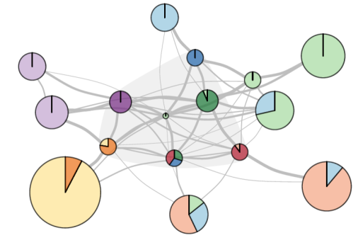
Figure 6: Network representation of the inferred clusters in the Infinito network. Each node denotes one cluster and edges are weighted by the estimated block probabilities. Node sizes are proportional to cluster cardinalities, while pie-charts represent compositions with respect to locale affiliations and leadership role; colors are the same as in Figure 5. To provide more direct insights, the composition with respect to role in the smaller-sized pie-charts is re-weighted to account for the fact that bosses are less frequent in the network relative to affiliates. Node positions are obtained via force-directed placement (Fruchterman and Reingold, 1991) to reflect strength of connections.

The above results are also confirmed in Figure 2, which clearly highlights the improved ability of the supervised gn process prior in learning the block structures that characterize the Infinito network. According to Figures 5 and 6, such modules suggest a nested partition structure mainly defined by the two macro-blocks of affiliates and bosses, which are further partitioned in sub-groups mostly coherent with the locale affiliation. The affiliates’ groups typically exhibit community patterns and connect to the hidden core mainly through the bosses of the corresponding locale, which in turn display weak assortative structures in the higher-level coordinating architecture among bosses of different locali.

Figure 7 confirms this result by showing how affiliates’ groups are typically characterized by high local transitivity and low betweenness, whereas clusters of bosses display the opposite behavior. This is a fundamental finding which provides new empirical evidence on the attempt of ’Ndrangheta bosses to address the tradeoff between efficiency and security (Morselli, Giguère and Petit, 2007) via the creation of low-sized, sparse and secure core groups with a high betweenness that favors the flow of information towards larger and dense groups of affiliates, which guarantee efficiency. Besides these recurring architectures, the flexibility of esbm is also able to account for other informative local deviations. For instance, the first group in Figure 5 comprises affiliates from different locali, who were found in judicial acts¹ to have peripheral roles. Similarly, the moderate block-connectivity patterns between the purple locale and the yellow one in Figures 5–6, are consistent with the fact that the latter was created as a branching of the former¹. The green locale has instead more complex block structures among affiliates, with a fragmentation in various subgroups denoting middle-level leadership positions. According to the judicial acts¹, these positions typically refer to authority roles in overseeing criminal actions or in guaranteeing coordination between La Lombardia and the leading ’Ndrangheta families in Calabria. Similar roles are covered also by the small fraction of affiliates allocated to groups of bosses. Among these affiliates it is worth highlighting the suspect allocated to the single-node cluster with the most central position in Figure 6. While not being classified as a boss in the judicial acts¹, such a suspect is a senior member of high rank in the organization with fundamental mediating roles between all the locali, and with the leading ’Ndrangheta families in Calabria. Hence, the actual position of such an affiliate in the vertical structure of La Lombardia may be much higher than currently reported.

Figure 7: Scatterplot of the average betweenness and local transitivity for each estimated cluster under the supervised gn prior. Sizes are proportional to cluster cardinalities, whereas the color of each point is set equal to the one occupying the largest portion of the associated pie-chart in Figure 6. Circles and squares represent groups mostly referring to affiliates and bosses, respectively, while the $\Delta$ and $+$ symbols denote cluster-specific measures computed from the partitions estimated under the Louvain algorithm (Blondel et al., 2008) ($\Delta$) and spectral clustering (Von Luxburg, 2007) ($+$).

As shown in Figures 2 and 7, all the above structures cannot be inferred under state-of-the-art alternatives, and therefore open new avenues to obtain a substantially improved understanding of the criminal network organization under esbm, along with refined predictive strategies for incoming affiliates. In particular, the predictive methods in Section 3.2 applied to the $34$ held-out suspects in the Infinito network crucially allow to recognize the role of incoming criminals without the need to use external information, that may not be available when a suspect is first observed. In fact, classifying the $34$ held-out suspects via (13) with an unsupervised gn prior favors allocation of new affiliates to current clusters characterized by high normalized local transitivity and low normalized betweenness, whereas incoming bosses are assigned to groups with much lower difference among these quantities. More specifically, the average difference between the two measures is $0.884$ for the held-out affiliates, and $0.204$ for the held-out bosses.

6 Discussion and future research directions

Criminal networks provide a fundamental field of application where the advancements in network science can have a major societal impact. However, despite the relevance of such studies, there has been limited consideration of criminal networks in the statistical literature, and the focus has been largely on restrictive methods that offer limited knowledge on the internal structure of criminal organizations. To cover this gap, we proposed esbms as a broad class of realistic models that unifies most existing sbms via Gibbs-type priors. Besides providing a single methodological, theoretical and computational framework for various sbms, such a generalization facilitates the proposal of new models by exploring alternative options within the Gibbs-type class, and allows natural inclusion of attributes via connections with ppms. Both aspects are fundamental to investigate criminal networks. For example, we have shown in simulations that the Gnedin process, which to the best of our knowledge had never been used in sbms, yields a suitable prior for partition structures in organized crime, and can improve the performance of already-implemented dp, py and dm in various realistic criminal networks where routine strategies, such as community detection and spectral clustering, fail. The motivating Infinito network application clarifies the benefits of our extended class of models and methods, providing formal unprecedented empirical evidence to several forensic theories on the internal functioning of complex criminal organizations, such as ’Ndrangheta.

The present work offers also many future directions of research. For example, the highly general and modular structure of esbms motivates application to modern real-world networks beyond criminal ones, and facilitates extensions to directed, bipartite and weighted networks. To address this goal, it is sufficient to substitute the beta-binomial likelihood in (1) with suitable ones, such as gamma-Poisson for count edges and Gaussian–Gaussian for continuous ones. Other types of suspect attributes beyond categorical ones can also be easily included leveraging the default choices suggested by Müller, Quintana and Rosner (2011) for $p(\cdot)$ in (4) under continuous, ordinal and count-type attributes. Additional applications to other criminal networks and further extensions to alternative representations, such as the mixed membership sbm (Airoldi et al., 2008; Ranciati, Vinciotti and Wit, 2020) and degree corrected sbm (Karrer and Newman, 2011), are also worthy of exploration. Despite the relevance of such constructions, we shall emphasize that while esbm preserves interpretability and parsimony by avoiding mixed membership structures, it still allows quantification of uncertainty in the degree of affiliation to different groups via formal inference on the posterior similarity matrix and on the credible bounds. Finally, although studying the coverage properties of the credible balls presented in Section 3.2 is still an ongoing area of research that goes beyond the scope of the present article (Wade and Ghahramani, 2018), it would be of interest to empirically check such properties within the esbm context.

References

- Abbe (2017) {barticle}[author] \bauthor\bsnmAbbe, \bfnmEmmanuel\binitsE. (\byear2017). \btitleCommunity detection and stochastic block models: Recent developments. \bjournalJournal of Machine Learning Research \bvolume18 \bpages6446–6531. \endbibitem
- Agreste et al. (2016) {barticle}[author] \bauthor\bsnmAgreste, \bfnmSanta\binitsS., \bauthor\bsnmCatanese, \bfnmSalvatore\binitsS., \bauthor\bsnmDe Meo, \bfnmPasquale\binitsP., \bauthor\bsnmFerrara, \bfnmEmilio\binitsE. and \bauthor\bsnmFiumara, \bfnmGiacomo\binitsG. (\byear2016). \btitleNetwork structure and resilience of mafia syndicates. \bjournalInformation Sciences \bvolume351 \bpages30–47. \endbibitem
- Airoldi et al. (2008) {barticle}[author] \bauthor\bsnmAiroldi, \bfnmEdoardo M.\binitsE. M., \bauthor\bsnmBlei, \bfnmDavid M.\binitsD. M., \bauthor\bsnmFienberg, \bfnmStephen E.\binitsS. E. and \bauthor\bsnmXing, \bfnmEric P.\binitsE. P. (\byear2008). \btitleMixed membership stochastic blockmodels. \bjournalJournal of Machine Learning Research \bvolume9 \bpages1981–2014. \endbibitem
- Amini et al. (2013) {barticle}[author] \bauthor\bsnmAmini, \bfnmArash A\binitsA. A., \bauthor\bsnmChen, \bfnmAiyou\binitsA., \bauthor\bsnmBickel, \bfnmPeter J\binitsP. J. and \bauthor\bsnmLevina, \bfnmElizaveta\binitsE. (\byear2013). \btitlePseudo-likelihood methods for community detection in large sparse networks. \bjournalThe Annals of Statistics \bvolume41 \bpages2097–2122. \endbibitem
- Athreya et al. (2017) {barticle}[author] \bauthor\bsnmAthreya, \bfnmAvanti\binitsA., \bauthor\bsnmFishkind, \bfnmDonniell E\binitsD. E., \bauthor\bsnmTang, \bfnmMinh\binitsM., \bauthor\bsnmPriebe, \bfnmCarey E\binitsC. E., \bauthor\bsnmPark, \bfnmYoungser\binitsY., \bauthor\bsnmVogelstein, \bfnmJoshua T\binitsJ. T., \bauthor\bsnmLevin, \bfnmKeith\binitsK., \bauthor\bsnmLyzinski, \bfnmVince\binitsV. and \bauthor\bsnmQin, \bfnmYichen\binitsY. (\byear2017). \btitleStatistical inference on random dot product graphs: A survey. \bjournalJournal of Machine Learning Research \bvolume18 \bpages8393–8484. \endbibitem
- Bickel et al. (2013) {barticle}[author] \bauthor\bsnmBickel, \bfnmPeter\binitsP., \bauthor\bsnmChoi, \bfnmDavid\binitsD., \bauthor\bsnmChang, \bfnmXiangyu\binitsX. and \bauthor\bsnmZhang, \bfnmHai\binitsH. (\byear2013). \btitleAsymptotic normality of maximum likelihood and its variational approximation for stochastic blockmodels. \bjournalThe Annals of Statistics \bvolume41 \bpages1922–1943. \endbibitem
- Binkiewicz, Vogelstein and Rohe (2017) {barticle}[author] \bauthor\bsnmBinkiewicz, \bfnmNorbert\binitsN., \bauthor\bsnmVogelstein, \bfnmJoshua T\binitsJ. T. and \bauthor\bsnmRohe, \bfnmKarl\binitsK. (\byear2017). \btitleCovariate-assisted spectral clustering. \bjournalBiometrika \bvolume104 \bpages361–377. \endbibitem
- Blondel et al. (2008) {barticle}[author] \bauthor\bsnmBlondel, \bfnmVincent D\binitsV. D., \bauthor\bsnmGuillaume, \bfnmJean Loup\binitsJ. L., \bauthor\bsnmLambiotte, \bfnmRenaud\binitsR. and \bauthor\bsnmLefebvre, \bfnmEtienne\binitsE. (\byear2008). \btitleFast unfolding of communities in large networks. \bjournalJournal of Statistical Mechanics \bvolume10 \bpagesP10008. \endbibitem
- Calderoni, Brunetto and Piccardi (2017) {barticle}[author] \bauthor\bsnmCalderoni, \bfnmFrancesco\binitsF., \bauthor\bsnmBrunetto, \bfnmDomenico\binitsD. and \bauthor\bsnmPiccardi, \bfnmCarlo\binitsC. (\byear2017). \btitleCommunities in criminal networks: A case study. \bjournalSocial Networks \bvolume48 \bpages116–125. \endbibitem
- Calderoni and Piccardi (2014) {binproceedings}[author] \bauthor\bsnmCalderoni, \bfnmFrancesco\binitsF. and \bauthor\bsnmPiccardi, \bfnmCarlo\binitsC. (\byear2014). \btitleUncovering the structure of criminal organizations by community analysis: The Infinito network. In \bbooktitle2014 Tenth International Conference on Signal-Image Technology and Internet-Based Systems \bpages301–308. \bpublisherIEEE. \endbibitem
- Campana (2016) {barticle}[author] \bauthor\bsnmCampana, \bfnmPaolo\binitsP. (\byear2016). \btitleExplaining criminal networks: Strategies and potential pitfalls. \bjournalMethodological Innovations \bvolume9 \bpages1–10. \endbibitem
- Campana and Varese (2020) {barticle}[author] \bauthor\bsnmCampana, \bfnmPaolo\binitsP. and \bauthor\bsnmVarese, \bfnmFederico\binitsF. (\byear2020). \btitleStudying organized crime networks: Data sources, boundaries and the limits of structural measures. \bjournalSocial Networks \bpagesIn press. \endbibitem
- Carley, Lee and Krackhardt (2002) {barticle}[author] \bauthor\bsnmCarley, \bfnmKathleen M\binitsK. M., \bauthor\bsnmLee, \bfnmJu-Sung\binitsJ.-S. and \bauthor\bsnmKrackhardt, \bfnmDavid\binitsD. (\byear2002). \btitleDestabilizing networks. \bjournalConnections \bvolume24 \bpages79–92. \endbibitem
- Catino (2014) {barticle}[author] \bauthor\bsnmCatino, \bfnmMaurizio\binitsM. (\byear2014). \btitleHow do mafias organize? Conflict and violence in three mafia organizations. \bjournalEuropean Journal of Sociology \bvolume55 \bpages177–220. \endbibitem
- Cavallaro et al. (2020) {barticle}[author] \bauthor\bsnmCavallaro, \bfnmLucia\binitsL., \bauthor\bsnmFicara, \bfnmAnnamaria\binitsA., \bauthor\bsnmDe Meo, \bfnmPasquale\binitsP., \bauthor\bsnmFiumara, \bfnmGiacomo\binitsG., \bauthor\bsnmCatanese, \bfnmSalvatore\binitsS., \bauthor\bsnmBagdasar, \bfnmOvidiu\binitsO., \bauthor\bsnmSong, \bfnmWei\binitsW. and \bauthor\bsnmLiotta, \bfnmAntonio\binitsA. (\byear2020). \btitleDisrupting resilient criminal networks through data analysis: The case of Sicilian Mafia. \bjournalPlos One \bvolume15 \bpages1–22. \endbibitem
- Chen and Lei (2018) {barticle}[author] \bauthor\bsnmChen, \bfnmKehui\binitsK. and \bauthor\bsnmLei, \bfnmJing\binitsJ. (\byear2018). \btitleNetwork cross-validation for determining the number of communities in network data. \bjournalJournal of the American Statistical Association \bvolume113 \bpages241–251. \endbibitem
- Côme and Latouche (2015) {barticle}[author] \bauthor\bsnmCôme, \bfnmEtienne\binitsE. and \bauthor\bsnmLatouche, \bfnmPierre\binitsP. (\byear2015). \btitleModel selection and clustering in stochastic block models based on the exact integrated complete data likelihood. \bjournalStatistical Modelling \bvolume15 \bpages564–589. \endbibitem
- Côme et al. (2021) {barticle}[author] \bauthor\bsnmCôme, \bfnmEtienne\binitsE., \bauthor\bsnmJouvin, \bfnmNicolas\binitsN., \bauthor\bsnmLatouche, \bfnmPierre\binitsP. and \bauthor\bsnmBouveyron, \bfnmCharles\binitsC. (\byear2021). \btitleHierarchical clustering with discrete latent variable models and the integrated classification likelihood. \bjournalAdvances in Data Analysis and Classification \bvolume15 \bpages957–986. \endbibitem
- De Blasi, Lijoi and Prünster (2013) {barticle}[author] \bauthor\bsnmDe Blasi, \bfnmPierpaolo\binitsP., \bauthor\bsnmLijoi, \bfnmAntonio\binitsA. and \bauthor\bsnmPrünster, \bfnmIgor\binitsI. (\byear2013). \btitleAn asymptotic analysis of a class of discrete nonparametric priors. \bjournalStatistica Sinica \bvolume23 \bpages1299–1321. \endbibitem
- De Blasi et al. (2015) {barticle}[author] \bauthor\bsnmDe Blasi, \bfnmPierpaolo\binitsP., \bauthor\bsnmFavaro, \bfnmStefano\binitsS., \bauthor\bsnmLijoi, \bfnmAntonio\binitsA., \bauthor\bsnmMena, \bfnmRamsés H\binitsR. H., \bauthor\bsnmPrünster, \bfnmIgor\binitsI. and \bauthor\bsnmRuggiero, \bfnmMatteo\binitsM. (\byear2015). \btitleAre Gibbs–type priors the most natural generalization of the Dirichlet process? \bjournalIEEE Transactions on Pattern Analysis and Machine Intelligence \bvolume37 \bpages212–229. \endbibitem
- Diviák (2019) {barticle}[author] \bauthor\bsnmDiviák, \bfnmTomáš\binitsT. (\byear2019). \btitleKey aspects of covert networks data collection: Problems, challenges, and opportunities. \bjournalSocial Networks \bpagesIn press. \endbibitem
- Faust and Tita (2019) {barticle}[author] \bauthor\bsnmFaust, \bfnmKatherine\binitsK. and \bauthor\bsnmTita, \bfnmGeorge E\binitsG. E. (\byear2019). \btitleSocial networks and crime: Pitfalls and promises for advancing the field. \bjournalAnnual Review of Criminology \bvolume2 \bpages99–122. \endbibitem
- Ferrara et al. (2014) {barticle}[author] \bauthor\bsnmFerrara, \bfnmEmilio\binitsE., \bauthor\bsnmDe Meo, \bfnmPasquale\binitsP., \bauthor\bsnmCatanese, \bfnmSalvatore\binitsS. and \bauthor\bsnmFiumara, \bfnmGiacomo\binitsG. (\byear2014). \btitleDetecting criminal organizations in mobile phone networks. \bjournalExpert Systems with Applications \bvolume41 \bpages5733–5750. \endbibitem
- Fortunato and Hric (2016) {barticle}[author] \bauthor\bsnmFortunato, \bfnmSanto\binitsS. and \bauthor\bsnmHric, \bfnmDarko\binitsD. (\byear2016). \btitleCommunity detection in networks: A user guide. \bjournalPhysics Reports \bvolume659 \bpages1–44. \endbibitem
- Fosdick et al. (2019) {barticle}[author] \bauthor\bsnmFosdick, \bfnmBailey K\binitsB. K., \bauthor\bsnmMcCormick, \bfnmTyler H\binitsT. H., \bauthor\bsnmMurphy, \bfnmThomas Brendan\binitsT. B., \bauthor\bsnmNg, \bfnmTin Lok James\binitsT. L. J. and \bauthor\bsnmWestling, \bfnmTed\binitsT. (\byear2019). \btitleMultiresolution network models. \bjournalJournal of Computational and Graphical Statistics \bvolume28 \bpages185–196. \endbibitem
- Fruchterman and Reingold (1991) {barticle}[author] \bauthor\bsnmFruchterman, \bfnmThomas MJ\binitsT. M. and \bauthor\bsnmReingold, \bfnmEdward M\binitsE. M. (\byear1991). \btitleGraph drawing by force-directed placement. \bjournalSoftware: Practice and Experience \bvolume21 \bpages1129–1164. \endbibitem
- Gelman, Hwang and Vehtari (2014) {barticle}[author] \bauthor\bsnmGelman, \bfnmAndrew\binitsA., \bauthor\bsnmHwang, \bfnmJessica\binitsJ. and \bauthor\bsnmVehtari, \bfnmAki\binitsA. (\byear2014). \btitleUnderstanding predictive information criteria for Bayesian models. \bjournalStatistics and Computing \bvolume24 \bpages997–1016. \endbibitem
- Geng, Bhattacharya and Pati (2019) {barticle}[author] \bauthor\bsnmGeng, \bfnmJunxian\binitsJ., \bauthor\bsnmBhattacharya, \bfnmAnirban\binitsA. and \bauthor\bsnmPati, \bfnmDebdeep\binitsD. (\byear2019). \btitleProbabilistic community detection with unknown number of communities. \bjournalJournal of the American Statistical Association \bvolume114 \bpages893–905. \endbibitem
- Girvan and Newman (2002) {barticle}[author] \bauthor\bsnmGirvan, \bfnmMichelle\binitsM. and \bauthor\bsnmNewman, \bfnmMark EJ\binitsM. E. (\byear2002). \btitleCommunity structure in social and biological networks. \bjournalProceedings of the National Academy of Sciences \bvolume99 \bpages7821–7826. \endbibitem
- Gnedin (2010) {barticle}[author] \bauthor\bsnmGnedin, \bfnmAlexander\binitsA. (\byear2010). \btitleSpecies sampling model with finitely many types. \bjournalElectronic Communications in Probability \bvolume15 \bpages79–88. \endbibitem
- Gnedin and Pitman (2005) {barticle}[author] \bauthor\bsnmGnedin, \bfnmA.\binitsA. and \bauthor\bsnmPitman, \bfnmJim\binitsJ. (\byear2005). \btitleExchangeable Gibbs partitions and Stirling triangles. \bjournalZapiski Nauchnykh Seminarov, POMI \bvolume325 \bpages83–102. \endbibitem
- Gormley and Murphy (2010) {barticle}[author] \bauthor\bsnmGormley, \bfnmIsobel Claire\binitsI. C. and \bauthor\bsnmMurphy, \bfnmThomas Brendan\binitsT. B. (\byear2010). \btitleA mixture of experts latent position cluster model for social network data. \bjournalStatistical Methodology \bvolume7 \bpages385–405. \endbibitem
- Grassi et al. (2019) {barticle}[author] \bauthor\bsnmGrassi, \bfnmRosanna\binitsR., \bauthor\bsnmCalderoni, \bfnmF\binitsF., \bauthor\bsnmBianchi, \bfnmMonica\binitsM. and \bauthor\bsnmTorriero, \bfnmAnna\binitsA. (\byear2019). \btitleBetweenness to assess leaders in criminal networks: New evidence using the dual projection approach. \bjournalSocial Networks \bvolume56 \bpages23–32. \endbibitem
- Handcock, Raftery and Tantrum (2007) {barticle}[author] \bauthor\bsnmHandcock, \bfnmMark S\binitsM. S., \bauthor\bsnmRaftery, \bfnmAdrian E\binitsA. E. and \bauthor\bsnmTantrum, \bfnmJeremy M\binitsJ. M. (\byear2007). \btitleModel-based clustering for social networks. \bjournalJournal of the Royal Statistical Society: Series A \bvolume170 \bpages301–354. \endbibitem
- Hartigan (1990) {barticle}[author] \bauthor\bsnmHartigan, \bfnmJ. A.\binitsJ. A. (\byear1990). \btitlePartition models. \bjournalCommunications in Statistics - Theory and Methods \bvolume19 \bpages2745–2756. \endbibitem
- Holland, Laskey and Leinhardt (1983) {barticle}[author] \bauthor\bsnmHolland, \bfnmPaul W.\binitsP. W., \bauthor\bsnmLaskey, \bfnmKathryn Blackmond\binitsK. B. and \bauthor\bsnmLeinhardt, \bfnmSamuel\binitsS. (\byear1983). \btitleStochastic blockmodels: First steps. \bjournalSocial Networks \bvolume5 \bpages109–137. \endbibitem
- Karrer and Newman (2011) {barticle}[author] \bauthor\bsnmKarrer, \bfnmBrian\binitsB. and \bauthor\bsnmNewman, \bfnmMark EJ\binitsM. E. (\byear2011). \btitleStochastic blockmodels and community structure in networks. \bjournalPhysical Review E \bvolume83 \bpages1–11. \endbibitem
- Kass and Raftery (1995) {barticle}[author] \bauthor\bsnmKass, \bfnmRobert E\binitsR. E. and \bauthor\bsnmRaftery, \bfnmAdrian E\binitsA. E. (\byear1995). \btitleBayes factors. \bjournalJournal of the American Statistical Association \bvolume90 \bpages773–795. \endbibitem
- Kemp et al. (2006) {binproceedings}[author] \bauthor\bsnmKemp, \bfnmCharles\binitsC., \bauthor\bsnmTenenbaum, \bfnmJoshua B.\binitsJ. B., \bauthor\bsnmGriffiths, \bfnmThomas L.\binitsT. L., \bauthor\bsnmYamada, \bfnmTakeshi\binitsT. and \bauthor\bsnmUeda, \bfnmNaonori\binitsN. (\byear2006). \btitleLearning systems of concepts with an infinite relational model. In \bbooktitleProceedings of the 21st National Conference on Artificial Intelligence - Volume 1 \bpages381–388. \endbibitem
- Kim, Hughes and Sudderth (2012) {binproceedings}[author] \bauthor\bsnmKim, \bfnmDae\binitsD., \bauthor\bsnmHughes, \bfnmMichael\binitsM. and \bauthor\bsnmSudderth, \bfnmErick\binitsE. (\byear2012). \btitleThe nonparametric metadata dependent relational model. In \bbooktitleICML’12: Proceedings of the 29th International Conference on International Conference on Machine Learning \bpages1411–1418. \bpublisherIEEE. \endbibitem
- Krebs (2002) {barticle}[author] \bauthor\bsnmKrebs, \bfnmValdis E\binitsV. E. (\byear2002). \btitleMapping networks of terrorist cells. \bjournalConnections \bvolume24 \bpages43–52. \endbibitem
- Le (2012) {barticle}[author] \bauthor\bsnmLe, \bfnmVy\binitsV. (\byear2012). \btitleOrganised crime typologies: Structure, activities and conditions. \bjournalInternational Journal of Criminology and Sociology \bvolume1 \bpages121–131. \endbibitem
- Le and Levina (2015) {barticle}[author] \bauthor\bsnmLe, \bfnmCan M\binitsC. M. and \bauthor\bsnmLevina, \bfnmElizaveta\binitsE. (\byear2015). \btitleEstimating the number of communities in networks by spectral methods. \bjournalarXiv preprint arXiv:1507.00827. \endbibitem
- Lee and Wilkinson (2019) {barticle}[author] \bauthor\bsnmLee, \bfnmClement\binitsC. and \bauthor\bsnmWilkinson, \bfnmDarren J\binitsD. J. (\byear2019). \btitleA review of stochastic block models and extensions for graph clustering. \bjournalApplied Network Science \bvolume4 \bpages1–50. \endbibitem
- Legramanti, Rigon and Durante (2020) {barticle}[author] \bauthor\bsnmLegramanti, \bfnmS.\binitsS., \bauthor\bsnmRigon, \bfnmT.\binitsT. and \bauthor\bsnmDurante, \bfnmD.\binitsD. (\byear2020). \btitleBayesian testing for exogenous partition structures in stochastic block models. \bjournalSankhya A \bpagesIn press. \endbibitem
- Lei and Rinaldo (2015) {barticle}[author] \bauthor\bsnmLei, \bfnmJing\binitsJ. and \bauthor\bsnmRinaldo, \bfnmAlessandro\binitsA. (\byear2015). \btitleConsistency of spectral clustering in stochastic block models. \bjournalThe Annals of Statistics \bvolume43 \bpages215–237. \endbibitem
- Lenk (2009) {barticle}[author] \bauthor\bsnmLenk, \bfnmPeter\binitsP. (\byear2009). \btitleSimulation pseudo–bias correction to the harmonic mean estimator of integrated likelihoods. \bjournalJournal of Computational and Graphical Statistics \bvolume18 \bpages941–960. \endbibitem
- Li, Levina and Zhu (2020) {barticle}[author] \bauthor\bsnmLi, \bfnmTianxi\binitsT., \bauthor\bsnmLevina, \bfnmElizaveta\binitsE. and \bauthor\bsnmZhu, \bfnmJi\binitsJ. (\byear2020). \btitleNetwork cross-validation by edge sampling. \bjournalBiometrika \bvolume107 \bpages257–276. \endbibitem
- Lijoi, Mena and Prünster (2007a) {barticle}[author] \bauthor\bsnmLijoi, \bfnmAntonio\binitsA., \bauthor\bsnmMena, \bfnmRamsés H.\binitsR. H. and \bauthor\bsnmPrünster, \bfnmIgor\binitsI. (\byear2007a). \btitleControlling the reinforcement in Bayesian non-parametric mixture models. \bjournalJournal of the Royal Statistical Society. Series B \bvolume69 \bpages715–740. \endbibitem
- Lijoi, Mena and Prünster (2007b) {barticle}[author] \bauthor\bsnmLijoi, \bfnmAntonio\binitsA., \bauthor\bsnmMena, \bfnmRamsés H\binitsR. H. and \bauthor\bsnmPrünster, \bfnmIgor\binitsI. (\byear2007b). \btitleBayesian nonparametric estimation of the probability of discovering new species. \bjournalBiometrika \bvolume94 \bpages769–786. \endbibitem
- Lijoi, Prünster and Walker (2008) {barticle}[author] \bauthor\bsnmLijoi, \bfnmAntonio\binitsA., \bauthor\bsnmPrünster, \bfnmIgor\binitsI. and \bauthor\bsnmWalker, \bfnmStephen G\binitsS. G. (\byear2008). \btitleBayesian nonparametric estimators derived from conditional Gibbs structures. \bjournalThe Annals of Applied Probability \bvolume18 \bpages1519–1547. \endbibitem
- Liu et al. (2018) {barticle}[author] \bauthor\bsnmLiu, \bfnmFuchen\binitsF., \bauthor\bsnmChoi, \bfnmDavid\binitsD., \bauthor\bsnmXie, \bfnmLu\binitsL. and \bauthor\bsnmRoeder, \bfnmKathryn\binitsK. (\byear2018). \btitleGlobal spectral clustering in dynamic networks. \bjournalProceedings of the National Academy of Sciences \bvolume115 \bpages927–932. \endbibitem
- Magalingam, Davis and Rao (2015) {barticle}[author] \bauthor\bsnmMagalingam, \bfnmPritheega\binitsP., \bauthor\bsnmDavis, \bfnmStephen\binitsS. and \bauthor\bsnmRao, \bfnmAsha\binitsA. (\byear2015). \btitleUsing shortest path to discover criminal community. \bjournalDigital Investigation \bvolume15 \bpages1–17. \endbibitem
- Malm and Bichler (2011) {barticle}[author] \bauthor\bsnmMalm, \bfnmAili\binitsA. and \bauthor\bsnmBichler, \bfnmGisela\binitsG. (\byear2011). \btitleNetworks of collaborating criminals: Assessing the structural vulnerability of drug markets. \bjournalJournal of Research in Crime and Delinquency \bvolume48 \bpages271–297. \endbibitem
- Meilă (2007) {barticle}[author] \bauthor\bsnmMeilă, \bfnmMarina\binitsM. (\byear2007). \btitleComparing clusterings — an information based distance. \bjournalJournal of Multivariate Analysis \bvolume98 \bpages873–895. \endbibitem
- Miller and Harrison (2014) {barticle}[author] \bauthor\bsnmMiller, \bfnmJeffrey W\binitsJ. W. and \bauthor\bsnmHarrison, \bfnmMatthew T\binitsM. T. (\byear2014). \btitleInconsistency of Pitman-Yor process mixtures for the number of components. \bjournalJournal of Machine Learning Research \bvolume15 \bpages3333–3370. \endbibitem
- Miller and Harrison (2018) {barticle}[author] \bauthor\bsnmMiller, \bfnmJeffrey W\binitsJ. W. and \bauthor\bsnmHarrison, \bfnmMatthew T\binitsM. T. (\byear2018). \btitleMixture models with a prior on the number of components. \bjournalJournal of the American Statistical Association \bvolume113 \bpages340–356. \endbibitem
- Morselli (2009) {barticle}[author] \bauthor\bsnmMorselli, \bfnmCarlo\binitsC. (\byear2009). \btitleHells Angels in springtime. \bjournalTrends in Organized Crime \bvolume12 \bpages145–158. \endbibitem
- Morselli, Giguère and Petit (2007) {barticle}[author] \bauthor\bsnmMorselli, \bfnmCarlo\binitsC., \bauthor\bsnmGiguère, \bfnmCynthia\binitsC. and \bauthor\bsnmPetit, \bfnmKatia\binitsK. (\byear2007). \btitleThe efficiency/security trade-off in criminal networks. \bjournalSocial Networks \bvolume29 \bpages143–153. \endbibitem
- Müller, Quintana and Rosner (2011) {barticle}[author] \bauthor\bsnmMüller, \bfnmPeter\binitsP., \bauthor\bsnmQuintana, \bfnmFernando\binitsF. and \bauthor\bsnmRosner, \bfnmGary L\binitsG. L. (\byear2011). \btitleA product partition model with regression on covariates. \bjournalJournal of Computational and Graphical Statistics \bvolume20 \bpages260–278. \endbibitem
- Newman (2006) {barticle}[author] \bauthor\bsnmNewman, \bfnmMark EJ\binitsM. E. (\byear2006). \btitleModularity and community structure in networks. \bjournalProceedings of the National Academy of Sciences \bvolume103 \bpages8577–8582. \endbibitem
- Newman and Clauset (2016) {barticle}[author] \bauthor\bsnmNewman, \bfnmMark EJ\binitsM. E. and \bauthor\bsnmClauset, \bfnmAaron\binitsA. (\byear2016). \btitleStructure and inference in annotated networks. \bjournalNature Communications \bvolume7 \bpages1–11. \endbibitem
- Newman and Girvan (2004) {barticle}[author] \bauthor\bsnmNewman, \bfnmM. E. J.\binitsM. E. J. and \bauthor\bsnmGirvan, \bfnmM.\binitsM. (\byear2004). \btitleFinding and evaluating community structure in networks. \bjournalPhysical Review E \bvolume69 \bpages026113. \endbibitem
- Noroozi and Pensky (2020) {barticle}[author] \bauthor\bsnmNoroozi, \bfnmMajid\binitsM. and \bauthor\bsnmPensky, \bfnmMarianna\binitsM. (\byear2020). \btitleStatistical inference in heterogeneous block model. \bjournalarXiv preprint arXiv:2002.02610. \endbibitem
- Nowicki and Snijders (2001) {barticle}[author] \bauthor\bsnmNowicki, \bfnmKrzysztof\binitsK. and \bauthor\bsnmSnijders, \bfnmTom A. B\binitsT. A. B. (\byear2001). \btitleEstimation and prediction for stochastic blockstructures. \bjournalJournal of the American Statistical Association \bvolume96 \bpages1077–1087. \endbibitem
- Olhede and Wolfe (2014) {barticle}[author] \bauthor\bsnmOlhede, \bfnmSofia C\binitsS. C. and \bauthor\bsnmWolfe, \bfnmPatrick J\binitsP. J. (\byear2014). \btitleNetwork histograms and universality of blockmodel approximation. \bjournalProceedings of the National Academy of Sciences \bvolume111 \bpages14722–14727. \endbibitem
- Pajor (2017) {barticle}[author] \bauthor\bsnmPajor, \bfnmAnna\binitsA. (\byear2017). \btitleEstimating the marginal likelihood using the arithmetic mean identity. \bjournalBayesian Analysis \bvolume12 \bpages261–287. \endbibitem
- Paoli (2007) {barticle}[author] \bauthor\bsnmPaoli, \bfnmLetizia\binitsL. (\byear2007). \btitleMafia and organised crime in Italy: The unacknowledged successes of law enforcement. \bjournalWest European Politics \bvolume30 \bpages854–880. \endbibitem
- Park and Dunson (2010) {barticle}[author] \bauthor\bsnmPark, \bfnmAuthor Ju-hyun\binitsA. J.-h. and \bauthor\bsnmDunson, \bfnmDavid B\binitsD. B. (\byear2010). \btitleBayesian generalized product partition model. \bjournalStatistica Sinica \bvolume20 \bpages1203–1226. \endbibitem
- Quintana and Iglesias (2003) {barticle}[author] \bauthor\bsnmQuintana, \bfnmFernando A.\binitsF. A. and \bauthor\bsnmIglesias, \bfnmPilar L.\binitsP. L. (\byear2003). \btitleBayesian clustering and product partition models. \bjournalJournal of the Royal Statistical Society. Series B \bvolume65 \bpages557–574. \endbibitem
- Raftery et al. (2007) {barticle}[author] \bauthor\bsnmRaftery, \bfnmAdrian E\binitsA. E., \bauthor\bsnmNewton, \bfnmMichael A\binitsM. A., \bauthor\bsnmSatagopan, \bfnmJaya M\binitsJ. M. and \bauthor\bsnmKrivitsky, \bfnmPavel N\binitsP. N. (\byear2007). \btitleEstimating the integrated likelihood via posterior simulation using the harmonic mean identity. \bjournalBayesian Statistics \bvolume8 \bpages1–45. \endbibitem
- Ranciati, Vinciotti and Wit (2020) {barticle}[author] \bauthor\bsnmRanciati, \bfnmSaverio\binitsS., \bauthor\bsnmVinciotti, \bfnmVeronica\binitsV. and \bauthor\bsnmWit, \bfnmErnst C\binitsE. C. (\byear2020). \btitleIdentifying overlapping terrorist cells from the Noordin Top actor–event network. \bjournalThe Annals of Applied Statistics \bvolume14 \bpages1516–1534. \endbibitem
- Rastelli, Latouche and Friel (2018) {barticle}[author] \bauthor\bsnmRastelli, \bfnmRiccardo\binitsR., \bauthor\bsnmLatouche, \bfnmPierre\binitsP. and \bauthor\bsnmFriel, \bfnmNial\binitsN. (\byear2018). \btitleChoosing the number of groups in a latent stochastic blockmodel for dynamic networks. \bjournalNetwork Science \bvolume6 \bpages469–493. \endbibitem
- Rohe, Chatterjee and Yu (2011) {barticle}[author] \bauthor\bsnmRohe, \bfnmKarl\binitsK., \bauthor\bsnmChatterjee, \bfnmSourav\binitsS. and \bauthor\bsnmYu, \bfnmBin\binitsB. (\byear2011). \btitleSpectral clustering and the high-dimensional stochastic blockmodel. \bjournalThe Annals of Statistics \bvolume39 \bpages1878–1915. \endbibitem
- Saldana, Yu and Feng (2017) {barticle}[author] \bauthor\bsnmSaldana, \bfnmD Franco\binitsD. F., \bauthor\bsnmYu, \bfnmYi\binitsY. and \bauthor\bsnmFeng, \bfnmYang\binitsY. (\byear2017). \btitleHow many communities are there? \bjournalJournal of Computational and Graphical Statistics \bvolume26 \bpages171–181. \endbibitem
- Sangkaran, Abdullah and Jhanjhi (2020) {barticle}[author] \bauthor\bsnmSangkaran, \bfnmTheyvaa\binitsT., \bauthor\bsnmAbdullah, \bfnmAzween\binitsA. and \bauthor\bsnmJhanjhi, \bfnmNZ\binitsN. (\byear2020). \btitleCriminal community detection based on isomorphic subgraph analytics. \bjournalOpen Computer Science \bvolume10 \bpages164–174. \endbibitem
- Sarkar and Bickel (2015) {barticle}[author] \bauthor\bsnmSarkar, \bfnmPurnamrita\binitsP. and \bauthor\bsnmBickel, \bfnmPeter J\binitsP. J. (\byear2015). \btitleRole of normalization in spectral clustering for stochastic blockmodels. \bjournalThe Annals of Statistics \bvolume43 \bpages962–990. \endbibitem
- Schmidt and Morup (2013) {barticle}[author] \bauthor\bsnmSchmidt, \bfnmMikkel N\binitsM. N. and \bauthor\bsnmMorup, \bfnmMorten\binitsM. (\byear2013). \btitleNonparametric Bayesian modeling of complex networks: An introduction. \bjournalIEEE Signal Processing Magazine \bvolume30 \bpages110–128. \endbibitem
- Sengupta and Chen (2018) {barticle}[author] \bauthor\bsnmSengupta, \bfnmSrijan\binitsS. and \bauthor\bsnmChen, \bfnmYuguo\binitsY. (\byear2018). \btitleA block model for node popularity in networks with community structure. \bjournalJournal of the Royal Statistical Society: Series B \bvolume80 \bpages365–386. \endbibitem
- Spiegelhalter et al. (2002) {barticle}[author] \bauthor\bsnmSpiegelhalter, \bfnmDavid J\binitsD. J., \bauthor\bsnmBest, \bfnmNicola G\binitsN. G., \bauthor\bsnmCarlin, \bfnmBradley P\binitsB. P. and \bauthor\bsnmVan Der Linde, \bfnmAngelika\binitsA. (\byear2002). \btitleBayesian measures of model complexity and fit. \bjournalJournal of the Royal Statistical Society: Series B \bvolume64 \bpages583–639. \endbibitem
- Stanley et al. (2019) {barticle}[author] \bauthor\bsnmStanley, \bfnmNatalie\binitsN., \bauthor\bsnmBonacci, \bfnmThomas\binitsT., \bauthor\bsnmKwitt, \bfnmRoland\binitsR., \bauthor\bsnmNiethammer, \bfnmMarc\binitsM. and \bauthor\bsnmMucha, \bfnmPeter J\binitsP. J. (\byear2019). \btitleStochastic block models with multiple continuous attributes. \bjournalApplied Network Science \bvolume4 \bpages1–22. \endbibitem
- Sussman et al. (2012) {barticle}[author] \bauthor\bsnmSussman, \bfnmDaniel L\binitsD. L., \bauthor\bsnmTang, \bfnmMinh\binitsM., \bauthor\bsnmFishkind, \bfnmDonniell E\binitsD. E. and \bauthor\bsnmPriebe, \bfnmCarey E\binitsC. E. (\byear2012). \btitleA consistent adjacency spectral embedding for stochastic blockmodel graphs. \bjournalJournal of the American Statistical Association \bvolume107 \bpages1119–1128. \endbibitem
- Tallberg (2004) {barticle}[author] \bauthor\bsnmTallberg, \bfnmChristian\binitsC. (\byear2004). \btitleA Bayesian approach to modeling stochastic blockstructures with covariates. \bjournalJournal of Mathematical Sociology \bvolume29 \bpages1–23. \endbibitem
- Von Luxburg (2007) {barticle}[author] \bauthor\bsnmVon Luxburg, \bfnmUlrike\binitsU. (\byear2007). \btitleA tutorial on spectral clustering. \bjournalStatistics and Computing \bvolume17 \bpages395–416. \endbibitem
- Wade and Ghahramani (2018) {barticle}[author] \bauthor\bsnmWade, \bfnmSara\binitsS. and \bauthor\bsnmGhahramani, \bfnmZoubin\binitsZ. (\byear2018). \btitleBayesian cluster analysis: Point estimation and credible balls. \bjournalBayesian Analysis \bvolume13 \bpages559–626. \endbibitem
- Wang and Bickel (2017) {barticle}[author] \bauthor\bsnmWang, \bfnmYX Rachel\binitsY. R. and \bauthor\bsnmBickel, \bfnmPeter J\binitsP. J. (\byear2017). \btitleLikelihood-based model selection for stochastic block models. \bjournalThe Annals of Statistics \bvolume45 \bpages500–528. \endbibitem
- Wang et al. (2018) {barticle}[author] \bauthor\bsnmWang, \bfnmYu-Bo\binitsY.-B., \bauthor\bsnmChen, \bfnmMing-Hui\binitsM.-H., \bauthor\bsnmKuo, \bfnmLynn\binitsL. and \bauthor\bsnmLewis, \bfnmPaul O\binitsP. O. (\byear2018). \btitleA new Monte Carlo method for estimating marginal likelihoods. \bjournalBayesian Analysis \bvolume13 \bpages311–333. \endbibitem
- Watanabe (2010) {barticle}[author] \bauthor\bsnmWatanabe, \bfnmSumio\binitsS. (\byear2010). \btitleAsymptotic equivalence of Bayes cross validation and widely applicable information criterion in singular learning theory. \bjournalJournal of Machine Learning Research \bvolume11 \bpages3571–3594. \endbibitem
- Watanabe (2013) {barticle}[author] \bauthor\bsnmWatanabe, \bfnmSumio\binitsS. (\byear2013). \btitleA widely applicable Bayesian information criterion. \bjournalJournal of Machine Learning Research \bvolume14 \bpages867–897. \endbibitem
- White and Murphy (2016) {barticle}[author] \bauthor\bsnmWhite, \bfnmArthur\binitsA. and \bauthor\bsnmMurphy, \bfnmThomas Brendan\binitsT. B. (\byear2016). \btitleMixed–membership of experts stochastic blockmodel. \bjournalNetwork Science \bvolume4 \bpages48–80. \endbibitem
- Xu et al. (2012) {binproceedings}[author] \bauthor\bsnmXu, \bfnmZhiqiang\binitsZ., \bauthor\bsnmKe, \bfnmYiping\binitsY., \bauthor\bsnmWang, \bfnmYi\binitsY., \bauthor\bsnmCheng, \bfnmHong\binitsH. and \bauthor\bsnmCheng, \bfnmJames\binitsJ. (\byear2012). \btitleA model-based approach to attributed graph clustering. In \bbooktitleProceedings of the 2012 ACM SIGMOD International Conference on Management of Data \bpages505–516. \endbibitem
- Yang, McAuley and Leskovec (2013) {binproceedings}[author] \bauthor\bsnmYang, \bfnmJaewon\binitsJ., \bauthor\bsnmMcAuley, \bfnmJulian\binitsJ. and \bauthor\bsnmLeskovec, \bfnmJure\binitsJ. (\byear2013). \btitleCommunity detection in networks with node attributes. In \bbooktitle2013 IEEE 13th International Conference on Data Mining \bpages1151–1156. \endbibitem
- Zhang, Levina and Zhu (2016) {barticle}[author] \bauthor\bsnmZhang, \bfnmYuan\binitsY., \bauthor\bsnmLevina, \bfnmElizaveta\binitsE. and \bauthor\bsnmZhu, \bfnmJi\binitsJ. (\byear2016). \btitleCommunity detection in networks with node features. \bjournalElectronic Journal of Statistics \bvolume10 \bpages3153–3178. \endbibitem
- Zhao, Du and Buntine (2017) {binproceedings}[author] \bauthor\bsnmZhao, \bfnmHe\binitsH., \bauthor\bsnmDu, \bfnmLan\binitsL. and \bauthor\bsnmBuntine, \bfnmWray\binitsW. (\byear2017). \btitleLeveraging node attributes for incomplete relational data. In \bbooktitleInternational Conference on Machine Learning \bpages4072–4081. \endbibitem
- Zhao, Levina and Zhu (2012) {barticle}[author] \bauthor\bsnmZhao, \bfnmYunpeng\binitsY., \bauthor\bsnmLevina, \bfnmElizaveta\binitsE. and \bauthor\bsnmZhu, \bfnmJi\binitsJ. (\byear2012). \btitleConsistency of community detection in networks under degree–corrected stochastic block models. \bjournalThe Annals of Statistics \bvolume40 \bpages2266–2292. \endbibitem
- Zhou and Amini (2019) {barticle}[author] \bauthor\bsnmZhou, \bfnmZhixin\binitsZ. and \bauthor\bsnmAmini, \bfnmArash A\binitsA. A. (\byear2019). \btitleAnalysis of spectral clustering algorithms for community detection: The general bipartite setting. \bjournalJournal of Machine Learning Research \bvolume20 \bpages47–1. \endbibitem