FTRANS: Energy-Efficient Acceleration of Transformers using FPGA

Abstract.

In natural language processing (NLP), the “Transformer” architecture was proposed as the first transduction model replying entirely on self-attention mechanisms without using sequence-aligned recurrent neural networks (RNNs) or convolution, and it achieved significant improvements for sequence to sequence tasks. The introduced intensive computation and storage of these pre-trained language representations has impeded their popularity into computation and memory constrained devices. The field-programmable gate array (FPGA) is widely used to accelerate deep learning algorithms for its high parallelism and low latency. However, the trained models are still too large to accommodate to an FPGA fabric. In this paper, we propose an efficient acceleration framework, Ftrans, for transformer-based large scale language representations. Our framework includes enhanced block-circulant matrix (BCM)-based weight representation to enable model compression on large-scale language representations at the algorithm level with few accuracy degradation, and an acceleration design at the architecture level. Experimental results show that our proposed framework significantly reduce the model size of NLP models by up to 16 times. Our FPGA design achieves 27.07$\times$ and 81 $\times$ improvement in performance and energy efficiency compared to CPU, and up to 8.80$\times$ improvement in energy efficiency compared to GPU.

1. Introduction

RNN and its variant Long Short-Term Memory (LSTM) unit (Hochreiter and Schmidhuber, 1997) and Gated Recurrent unit (GRU) (Cho et al., 2014) used to dominate in sequence modeling, language modeling and machine translation, etc. However, they in general lack efficiency in transmitting global information, due to the bottleneck in the memory (hidden state) and complicated bypassing logic (additive and derivative branches) where long range information is passed. In addition, the inherently sequential nature precludes parallelization within training examples through backpropagation, which is critical at longer sequence lengths (Kim et al., 2017).

To overcome the shortcomings in RNNs, the “Transformer” architecture was proposed as the first transduction model replying entirely on self-attention mechanisms without using sequence-aligned RNNs or convolution. It achieved notable improvements for sequence to sequence tasks (Vaswani et al., 2017). The breakthroughs and developments of new models have accelerated at an unprecedented pace since the attention mechanisms have become the mainstream in NLP domain with the invention of Transformer. Many transformer-based NLP language models like BERT (Devlin et al., 2018) and RoBERTa (Liu et al., 2019) introduced pretraining procedures to the transformer architecture and achieved record-breaking results on major NLP tasks, including question answering, sentiment analysis, and language inference.

Nevertheless, the introduced intensive computation and power footprint of these pre-trained language representations has impeded their popularity into computation and energy constrained as edge devices. Moreover, despite of the rapid advancement achieved by the recent transformer-based NLP models, there is a serious lack of studies on compressing these models for embedded and internet-of-things (IoT) devices.

In this paper, we propose an energy-efficient acceleration framework, Ftrans, for transformer-based large scale language representations using FPGA. Ftrans is comprised of an enhanced BCM-based method enabling model compression on language representations at the algorithm level, and an acceleration design at the architecture level. Our contributions are summarized as follows:

• Enhanced BCM-based model compression for Transformer. We address the accuracy degradation caused by traditional BCM compression, and propose an enhanced BCM-based compression to reduce the footprint of weights in Transformer. With small accuracy loss, Ftrans achieves up to 16 times compression ratio.

• Holistic optimization for Transformers on FPGA. Given the large size and complex data flow of transformer-based models, even with model compression, we still need to schedule the computation resources carefully to optimize latency and throughput. We propose a two stage optimization approach to mitigate the resource constraints and achieve high throughput.

• Low hardware footprint and low power (energy) consumption. We propose an FPGA architecture design to support the model compression technique and we develop a design automation and optimization technique. Overall, the proposed Ftrans achieves the lowest hardware cost and energy consumption in implementing Transformer and RoBERTa compared to CPU and GPU references.

Experimental results show that our proposed framework significantly reduce the size of NLP models by up to 16 times. Our FPGA design achieves 27.07$\times$ and 81 $\times$ improvement in performance and energy efficiency compared to CPU. The power consumption of GPU is up to 5.01$\times$ compared to that of FPGA, and we achieve up to 8.80$\times$ improvement in energy efficiency compared to GPU.

2. Related Work

Attention mechanisms have become an integral part of compelling sequence modeling and transduction models in various tasks (Kim et al., 2017). Evidence of NLP community moving towards attention-based models can be found by more attention-based neural networks developed by companies like Amazon (Kim and Kim, 2018), Facebook (Shi et al., 2018), and Salesforce (Bradbury and Socher, 2017). The novel approach of Transformer is the first model to eliminate recurrence completely with self-attention to handle the dependencies between input and output. BERT (Devlin et al., 2018) and RoBERTa (Liu et al., 2019) extend Transformer’s capacity from a sequence to sequence model to a general language model by introducing the pretraining procedure, and achieved state-of-the-art results on major NLP benchmarks. Although RNNs and Convolutional Neural Networks (CNNs) are being replaced by Transformer-based models in NLP community, there are only a few works that accelerate Transformers and focus on reducing the energy and power footprint, e.g., a case study of Transformer is presented in (xil, 2019) using one of the cutting-edge FPGA boards. However, it is noteworthy that (xil, 2019) targets at a specialized FPGA architecture, which employs High Bandwidth Memory (HBM) technology. Unlike the conventional FPGA, HBM is packaged directly within the FPGA fabric to alleviate the on chip memory constraint. However, work (xil, 2019) did not adopt model compression technique, and used the sequence length of 8 and 16, which are too short and not favorable in practise. The model details such as number of encoder/decoders, hidden size are also not listed.

3. Transformer Workload Analysis

The “Transformer” architecture is the heart for all state-of-the-art large scale language models. It has an encoder-decoder structure (Vaswani et al., 2017) as shown in Figure 1. The encoder maps a sequence of the input symbols $\mathbf{x}=({x}_{1};{x}_{2};{x}_{3};...;{x}_{n})$ to a sequence of continuous representations $\mathbf{z}=({z}_{1};{z}_{2};{z}_{3};...;{z}_{n})$. Given $\mathbf{x}$, the decoder then produces an output sequence $\mathbf{y}=({y}_{1};{y}_{2};{y}_{3};...;{y}_{m})$ of symbols one element per time step. For the next time step, the model takes the previously generated symbols as additional input when generating the next. The Transformer follows this overall architecture using stacked self-attention and fully-connected (FC) layers for both the encoder and decoder, shown in Figure 1.

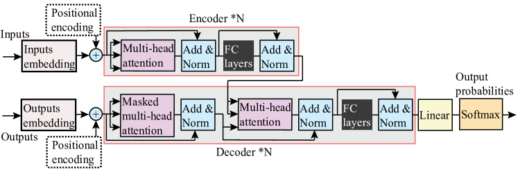
Figure 1. Model structure of Transformer.

Encoder: The encoder consists of a stack of $N$ identical layers. Each layer has two sub-layers. The first is a multi-head self-attention mechanism, and the second is a FC feed-forward network. There is a residual connection around each of the two sub-layers, followed by layer normalization.

Decoder: The decoder contains of a stack of $N$ identical layers. Within each layer, there are three sub-layers, where the third sub-layer is the same as the encoder. The inserted second sub-layer performs multi-head attention over the output of encoder stack. The first-sublayer utilizes masked multi-head attention, to ensure that predictions for position $i$ only depends on its previous positions.

3.1. Attention

The attention function can be described as mapping a query $\mathbf{q}$ and a set of keys $\mathbf{k}$ and values $\mathbf{v}$ pairs to an output $\mathbf{o}$ as shown in Figure 2 (a), named scaled dot-product attention, or single head attention.

3.1.1. Single Head Attention

In this paper, we select dot-product attention as the attention function since it is much faster and more space-efficient  (Vaswani et al., 2017). The input consists of queries and keys of dimension $d_{k}$, and values of dimension $d_{v}$. We denote $\sqrt{d_{k}}$ is the scaling factor for dot-product attention. We compute the dot products of the query with all keys, divide each by $\sqrt{d_{k}}$, and apply a softmax function to obtain the weights on the values. The attention function on $\mathbf{q}$, $\mathbf{k}$, and $\mathbf{v}$ can be computed simultaneously by concatenated into matrix $\mathbf{Q}$, $\mathbf{K}$, and $\mathbf{V}$, respectively. Accordingly, the output matrix $\mathbf{O}_{att}$ is:

(1) $$\small\mathbf{O}_{att}=Attention(\mathbf{Q},\mathbf{K},\mathbf{V})=softmax(\frac{\mathbf{QK}^{T}}{\sqrt{d_{k}}})\vspace{-0.2cm}$$

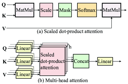
Figure 2. : (a) Scaled Dot-Product Attention. (b) Multi-Head Attention.

3.2. Multi-head Attention

Multi single-head attention are then concatenated as multi-head attention, as shown in Figure 2 (b). MultiHead ($\mathbf{Q}$, $\mathbf{K}$, $\mathbf{V}$) = Concat ($\text{Head}_{1},\cdots,\text{Head}_{h}$)$\times\mathbf{W}^{O}$, where the Head is defined as:

(2) $$\small\text{Head}_{i}=Attention(\mathbf{Q}\mathbf{W}_{i}^{Q},\mathbf{K}\mathbf{W}_{i}^{K},\mathbf{V}\mathbf{W}_{i}^{V})\vspace{-0.2cm}$$

where the projections are parameter matrices ${{\bf{W}}^{Q}_{i}}\in\mathbb{R}^{d_{model}\times d_{k}}$, ${{\bf{W}}^{K}_{i}}\in\mathbb{R}^{d_{model}\times d_{k}}$, and ${{\bf{W}}^{V}_{i}}\in\mathbb{R}^{d_{model}\times d_{v}}$. Multi-head attention enables the model to jointly attend to information from different representation subspaces at different positions (Vaswani et al., 2017).

In this work, we implement a shallow Transformer and a large scale Transformer, i.e., RoBERTa. The shallow Transformer has $h$ = 2 parallel attention layers with 4 attention heads and RoBERTa (base configuration) has 12 layers with 12 heads. For each head we use $d_{k}=d_{v}=d_{model}/h=200$ and $768$ for Transformer and RoBERTa, respectively.

4. Transformer Compression using Enhanced Block-Circulant Matrix

The introduced intensive computation and weight storage of large pre-trained language representations have brought challenges in hardware implementation. Therefore, model compression is a natural method to mitigate the these challenges.

4.1. Enhanced BCM-based Transformer

CirCNN (Ding et al., 2017) and C-LSTM (Wang et al., 2018) have adopted BCM for model compression on small to medium scale datasets in image classification and speech recognition, respectively, and achieved significant improvement in terms of performance and energy efficiency compared to the prior arts. Using this method, we can reduce weight storage by replacing the original weight matrix with one or multiple blocks of circulant matrices, where each row/column is the cyclic reformulation of the others. We use $b$ to represent the row/column size of each circulant matrix (or block size, FFT size). Suppose the shape of a weight matrix in Transformer (e.g., ${{\bf{W}}^{Q}_{i}},{{\bf{W}}^{K}_{i}},{{\bf{W}}^{V}_{i}})$ is $\textbf{W}\in\mathbb{R}^{m\times n}$, there will be $f\times g$ blocks after partitioning $\mathbf{W}$, where $f=m\div b$ and $g=n\div b$. Then $\mathbf{W}=[\mathbf{W}_{ij}]$, $i\in\{1\dots f\}$, $j\in\{1\dots g\}$.

The input $\mathbf{x}$ is also partitioned as $\mathbf{x}=[\mathbf{x}^{T}_{1},\mathbf{x}^{T}_{2},\dots,\mathbf{x}^{T}_{g}]^{T}$. In each BCM, only the first column/row is needed for storage and computation, and is termed the index vector, $\mathbf{p}_{ij}$. The theoretical foundation is derived in (Zhao et al., 2017), which demonstrates the universal approximation property and the error bounds of BCM-based neural networks are as efficient as general neural networks.

Prior works (Ding et al., 2017; Wang et al., 2018) have not investigated large-scale language representations. To further maintain the prediction accuracy, we use an enhanced BCM-based model compression. We modify the formulation of the index vector as follows:

(3) $$\footnotesize\mathbf{p}_{ij}=\begin{bmatrix}\frac{1}{b}\sum_{j=1}^{b}\mathbf{W}_{1j}\\ \frac{1}{b}\sum_{j=1}^{b}\mathbf{W}_{2j}\\ \dots\\ \frac{1}{b}\sum_{j=1}^{b}\mathbf{W}_{bj}\end{bmatrix}$$

where $\mathbf{W}_{ij}$ is a circulant matrix. We observe that in this way, we can better preserve the parameter information and maintain the overall prediction accuracy. The main reason is that prior works take the first column/row as the index vector, missing the effective representations for other rows/columns.

Based on the circulant convolution theorem (Pan, 2012; Smith, 2007), instead of directly performing the matrix-vector multiplication, we could use the fast Fourier transform (FFT)-based multiplication method, and it is equivalent to matrix-vector multiplication. The calculation of a BCM-based matrix-vector multiplication $\mathbf{W}_{ij}\mathbf{x}_{j}$ is: $\mathbf{W}_{ij}\mathbf{x}_{j}=\mathbf{p}_{ij}\circledast\mathbf{x}_{j}=\text{IFFT}\big{(}\text{FFT}(\mathbf{p}_{ij})\circ\text{FFT}(\mathbf{x}_{j})\big{)}$, where ‘$\circledast$ ’ represents circular convolution, and $\circ$ is element-wise multiplication. Therefore, the computational complexity is reduced from O($b^{2}$) to O($b\log b$).

5. Architecture

FPGA is widely used to accelerate deep learning models for its high parallelism and low latency. As large amount of transformer parameters exceed the on-chip memory or block RAM (BRAM) capacity on FPGA fabric, even with model compression technique, the full model cannot be stored on chip. To address the challenge, we partition a model into embedding layer and encoder/decoder stacks. The embedding layer contributes 30.89% of parameters. Essentially it is a look-up table which transforms discrete tokens into continuous space, the computation is less than that of encoder and decoder. Therefore, our basic idea is to off-load embedding layer to off-chip memory, thus it is possible to deploy the most computational intensive part, i.e. the encoder and decoder stack on chip, avoiding frequently access off-chip weights, hence to accelerate computation. Second, to mitigate the I/O constrain, we developed the inter-layer coarse grained pipelining, intra-layer fine grained pipeling, and computation scheduling.

5.1. Overall Hardware Architecture

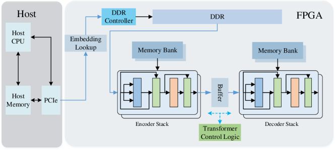
Figure 3. The overall hardware architecture on FPGA.

As shown in Figure 3, the proposed hardware architecture consists of computation units for encode/decoder computation, on-chip memory banks, a transformer controller, and an off-chip memory (DDR) and DDR controller. The transformer controller communicates with the host and controls all the modules in FPGA. The host PC loads the inputs (i.e., sentence pairs ) to the FPGA for inference through PCIE. On the FPGA part, given the tokenized sentences, the embedding look up module accesses DDR to fetch embeddings. Next, the embeddings will be fed into the pipelined encoder/decoder stacks to perform inference.

The computing units consist of multi-head attention, scaled dot product attention, point wise feed forward layer, linear, and add/norm. The transformer controller orchestrates the computing flow and data flow of inputs from PCIEs, BRAMs and computing units on the FPGA fabric. Since the encoder and decoder share same type of operations, so we first decompose them into different computing primitives, including matrix multiplication of different sizes, vectorized exponentials etc. The multi-head attention, linear, and add/norm modules are reconfigured to form as encoder or decoder under the transformer control logic. We have two pipeline strategies. For shallow networks, the entire network can be straightforwardly implemented, i.e. all layers can be implemented by dedicated FPGA resources. For the state-of-the-art designs such as BERT and RoBERTa, there are multiple encoders/decoders, hence the resource such as DSPs may not enough. In such cases, reuse of certain PE or entire encoder/decoder module are necessary.

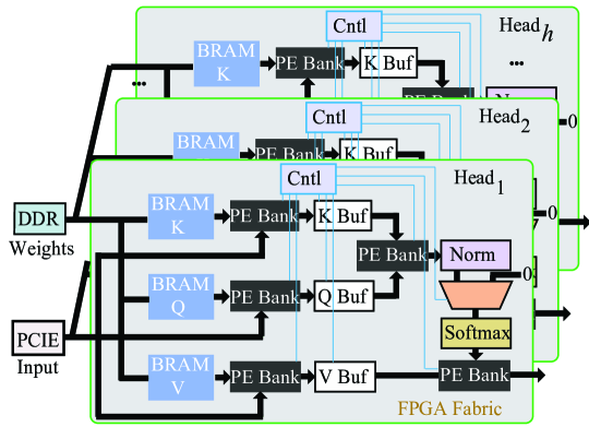
Figure 4. Multi-head attention ($\text{Head}_{1},\cdots,\text{Head}_{h}$) design.

5.2. Multi-Head Attention Design

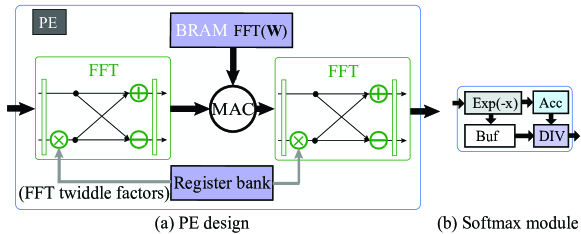
Figure 5. FFT/IFFT-based PE and softmax module design.

Multi-head attention includes multi-processing elements (named PE) banks, for matrix multiplication), buffers (K buf, Q buf, and V buf), a normalization module (Norm), a masking function for masked multi-head attention, and a softmax module as described in Equation (2) and shown in Fig. 4.

The input are fetched from DDR and fed into encoder pipeline, then multiplied with a set of query matrix $\mathbf{Q}$ and key matrix $\mathbf{K}$ stored on BRAMs. The intermediate results $\mathbf{Q}\mathbf{W}^{Q}$ and $\mathbf{K}\mathbf{W}^{K}$ are then propagated to the buffers (i.e., K buffer and Q buffer to store $\mathbf{K}\mathbf{W}^{K}$, and $\mathbf{Q}\mathbf{W}^{Q}$, respectively). Next, we compute the matrix multiplication of the values stored in the K buffer and W buffer. The product will be loaded to the normalization (Norm) module, i.e.,$\frac{product}{\sqrt{d_{k}}}$. After the softmax module, the results will be propagated to a PE bank to perform matrix multiplication with the matrix stored in $V$ Buf, i.e., $\mathbf{V}\mathbf{W}^{V}$. Each head will have a local controller to orchestrate the computing flow and data flow of PE banks and buffers. The local controller will also enable the multiplexer for masked multi-head attention with a goal of masking the future tokens in a sequence (setting to 0), to prevent the current output predictions from being able to see later into the sentence. To support masked multi-head attention, the local controller controls multiplexer to set future tokens to 0, such that current output predictions are not able to see later sequences. Decoder has one more multi-head attention, thus takes longer time to compute than encoder. In the case of decoder module has to be reused, to prevent encoder pipeline stall, a buffer is placed between the encoder and decoder stacks. The buffer also stores the output from the last encoder to support the residue connection.

5.3. PE Design and Softmax Module

We develop three different configurable PEs, which as PE-A, PE-B, and PE-FFT/IFFT. For the BCM-based matrix-vector multiplication in FC layers, we use FFT/IFFT-based processing elements (PE); for other layers, we use matrix-vector multiplication, i.e., PE-A and PE-B for different matrix sizes.

5.3.1. Matrix-vector multiplication-based PE

The major part of the PE-A or PE-B is a multiplier for matrix multiplication of different sizes. It also consists of two accumulators, dividers and exponential units to support scaling and softmax required by multi-head attention. The output of multipliers are fed into divider or accumulator as stream, hence scaling and softmax layer can be overlapped with matrix multiplication.

5.3.2. FFT/IFFT-based PE

Figure 5 shows the design of FFT/IFFT-based PE and softmax, including a FFT/IFFT kernel, an accumulator, and an adder. The accumulator is an adder tree with $N$ inputs (the size is chosen the same as the FFT/IFFT kernel size). We select Radix-2 Cooley Tukey algorithm (Johnsson and Krawitz, 1992) for FFT implementation.

5.3.3. Softmax Module

Figure 5 (b) shows the implementation of the softmax function $\text{softmax}(x)_{i}=\frac{exp(x_{i})}{\sum_{j}exp(x_{j}))}$. The exponential function ${exp(x_{i})}$ or ${exp(x_{j})}$ is expensive in resource consumption for FPGAs. We adopt piece-wise linear functions to estimate their outputs, in order to simultaneously reduce the resource consumption and maintain the accuracy. A buffer is used to store ${exp(x_{i})}$ and an accumulator is used to compute the summation of ${exp(x_{j})}$. Next, we perform the division and generate the softmax results.

6. Design Automation & Optimization

We developed a workflow to prototype and explore the hardware architecture. First, we generate a data dependency graph based on trained models to illustrate the computation flow. The operators in graph are scheduled to compose the pipeline under the design constraints, to achieve maximum throughput. At last, a code generator receives the scheduling results and generates the final C/C++ implementation, which can be fed into the commercial HLS tool for synthesis. Our target synthesis backend is Xilinx SDx.

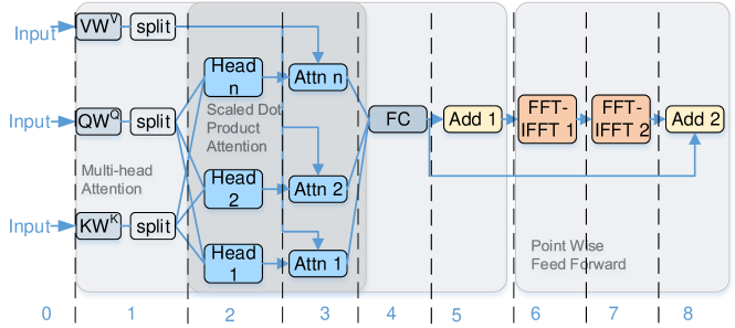
Figure 6. Data flow of major operations.

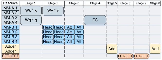
Figure 7. Fine grained operation scheduling

The major computationally intensive operations are shown in Figure 6. Other operations such as division and softmax consume much less time, and can be merged/overlapped with these major operations. The computation in different layers can be decomposed into common computing elements, i.e., PEs. The layers in same color can be performed by same PE, however, with unbalanced operations. For example, the time consumed by the $\mathbf{K}\mathbf{W}^{K}$, $\mathbf{Q}\mathbf{W}^{Q}$ and $\mathbf{V}\mathbf{W}^{V}$ is roughly 4 times of computation required by the $n$ heads. To improve the utilization of pipeline, it is desirable to let each layers consumes roughly the same time. This can be achieved by allocating more resources to the slowest layer. We adopt a two-stage optimization flow. In first stage, we find a resource scheme that can minimize the maximum time required by layers. In second stage, under such resource constrains, we optimize the scheduling of an individual encoder/decoder.

The optimization starts from a basic implementation of an individual encoder/decoder, i.e. no parallization nor resource reusing, such that we can obtain an estimation of resource consumption, number of operations and execution time of each layer, throughput obtained by unit number of resources. Then we will examine how much resource can be allocated to each encoder/decoder to minimize the execution time of the slowest layer:

(4) minimize $$\max(T_{1},T_{2},...,T_{n}),$$

subject to $$R_{F}[i]\geq M\sum_{j}{R_{j}[i]}+R_{misc}[i]$$

where $i\in(0,...,3)$, $j\in n$, $n$ is the number of layers, $M$ is the total number of encoder/decoder, $R_{F}=[R_{FF},R_{LUT},R_{DSP},R_{BRAM}]$ is on-chip resource constraints for look-up table (LUT), flip-flop (FF), digital signal processing unit (DSP), and BRAM, respectively. $T_{j}$ is the time required by the $j$-th layer. $R_{j}$ is resource utilization of the $j$-th layer, which is also represented as a vector: $R_{j}=[R^{j}_{FF},R^{j}_{LUT},R^{j}_{DSP},R^{j}_{BRAM}]$. $R_{misc}$ is the resource utilization of modules except encoder/decoder module, such as DDR controller, PCIE controller, etc. $T_{j}$ can be given as:

(5) $$T_{j}=\lceil{N^{i}_{op}}/(F_{j}\cdot K_{j})\rceil,j\in{n}\vspace{-0.3cm}$$

where $N^{i}_{op}$ is the number of operations required by the $j$-th layer. $K_{j}$ is resource allocation factor of the $j$-th layer. $F_{j}$ is the throughput of non-optimized design, which can be obtained empirically. Therefore, the throughput is:

(6) $$Throughput=freq/(n\cdot{max(T_{1},T_{2},...,T_{j})})$$

It finds the slowest layer, allocates more resources, then updates the resource consumption and execution time. If resource constraints are satisfied, we repeat this procedure until no more speedup. Then the algorithm will examine the fastest layer. If it takes significantly less time than the slowest layer, it is possible to allocate less resources for that layer, hence more resources can be assigned to the slowest layer. After this procedure, we obtain resource constraints, e.g. the No. of different PEs of an encoder and decoder. Under resource constraints, each layer may not have dedicated computation resource, hence matrix multipliers, adders, etc. have to be shared. Therefore, the computation has to be carefully scheduled to minimize the computation latency. The encoder/decoder can be represented as a Directed Acyclic Graph (DAG) – ${G}({V},{E})$, where ${V}$ is a set of vertices representing different computation, edges ${E}$ indicate the dependency. The available computation units such as PEs and adders are represented by a set ${Op}=\{PE-A1,PE-A2,...,Adder\}$. The algorithm used for operation scheduling takes ${G}$ and ${Op}$ as input, is shown in Algorithm 1.

Input: Dependency graph ${G}({V},{E})$, available PEs ${Op}=\{PE\_A1,PE\_A2,...,Adder\}$

Output: $C$ and designated $PE$ for each Layer

$Q=TOPO\_SORT({G}({V},{E}))$ $\backslash\backslash$ Topological sort to obtain priority queue of all layers

$P=Q[0]$ $\backslash\backslash$ List of layers to be scheduled

$E=\emptyset$ $\backslash\backslash$ List of layers being executed

$S=\emptyset$ $\backslash\backslash$ The final schedule result

$stage=0$

while $Q\neq\emptyset\land E\neq\emptyset$ do

       for $layer\in Q$ do

             if available $PE\exists Op$ for $layer$ then

                   $Q.pop()$

                   $Op.remove(PE)$

                   $E.push\_back((layer,PE))$

                   for $V\in NEIGHBOR(layer)$ do

                         $Q.push\_back(V)$

                        

                   end for

                  

            

       end for

      $stage+=1$

       for $layer,PE\in E$ do

             if $IS\_FINISHED(layer)==True$ then

                   $E.pop()$

                   $S.push\_back((layer,stage,PE))$

                   $Op.push\_back(PE)$

            

       end for

      

end while

return $S$

Algorithm 1 Pseudo-code for operation scheduling

7. Evaluation

7.1. Training of Transformer-Based Language Representation

In this section, we apply both enhanced BCM-based model compression on the linear layers, and adopt 16 fixed-point data representation for all the weights. We evaluate the accuracy impact with two representative Transformer structures, i.e., a shallow Transformer with both encoder and decoder, and a pretrained deep Transformer architecture - RoBERTa (base configuration) which only has encoder (Liu et al., 2019). The shallow Transformer is evaluated in a language modeling task, which is an unsupervised sequence-to-sequence problem that requires the decoder part. On the other hand, we run a RoBERTa on a sentiment classification task that is a supervised classification problem without the requirement for decoder block. The software is implemented in PyTorch deep learning framework (Paszke et al., 2017) and FairSeq sequence modeling toolkit (Ott et al., 2019). Table 1 summarizes the key parameters of the shallow Transformer and RoBERTa models in the experiments.

Table 1. Key parameters of Shallow Transformer and RoBERTa

Model	Transformer	Transformer	Hidden	Attention	Total
Configuration	Structure	Layers	Size	Heads	Params
Shallow Transformer	encoder-decoder	2	200	4	6M
RoBERTa (base config.)	encoder only	12	768	12	125M

7.1.1. Finetuned RoBERTa for Sentiment Classification

We evaluate the proposed model compression method for finetuned RoBERTa (Liu et al., 2019) on IMDB movie review sentiment classification (Maas et al., 2011) to shed some light on training trial reductions. Starting from the saved state of pretrained models in work (Liu et al., 2019), we finetune the model until it reaches to its best validation accuracy at 95.7%. To maintain overall accuracy, we compress partial layers. The process suppresses randomness by using a deterministic seed. Thus the accuracy difference between the original RoBERTa and compressed version is sorely contributed by the compression techniques.

7.1.2. Shallow Transformer

Language modeling task takes a sequence of words as input and determines how likely that sequence is the actual human language. We consider the popular WikiText-2 dataset (Merity et al., [n. d.]) in this experiment, which contains 2M training tokens with a vocabulary size of 33k. A shallow Transformer model with 4 attention heads and 200 hidden dimension is established.

The baseline and model compression results of shallow Transformer and RoBERTa on WikiText-2 and IMDB review are shown in Table 2, respectively. We compress the models using enhanced BCM-based method with block size of 4 or 8. From Table 2, we observe that for the shallow Transformer, thers is no accuracy loss with block size of 4 and only 0.6% accuracy loss with block size of 8. The RoBERTa, on the other hand, incurs 4.2% and 4.3% accuracy drop after model compression using 4 and 8 block size, respectively. We also observe that changing from 32-bit floating point to 16-bit fixed point will not cause accuracy loss. The comparable accuracy between the original model and the weight compressed version demonstrates the effectiveness of the proposed model compression method.

Table 2. Comparison among different model configurations

ID	Network	Block	WikiText-2	ACC loss	ACC loss
	Type	Size	(ACC) %	with BCM (%)	with BCM & Quant. (%)
1	Shallow Transformer	$-$	91.3	$-$	$-$
2	Shallow Transformer	$4$	90.7	0.6	0
3	Shallow Transformer	$8$	90.7	0.6	0.6
4	Shallow Transformer	$16$	90.0	1.3	0.6
ID	Network	Block	IMDB	ACC loss	ACC loss
	Type	Size	(ACC)%	with BCM (%)	with BCM & Quant. (%)
4	RoBERTa (base)	$-$	95.7	$-$	$-$
5	RoBERTa (base)	$4$	91.5	4.2	4.3
6	RoBERTa (base)	$8$	91.4	4.3	4.3

7.2. Performance and Energy Efficiency

Table 3. Comparison among different model configurations

Shallow Transformer
Batch Size	DSP	FF	LUT	Latency (ms)	Power (W)	Throughput (FPS)
1	5647	304012	268933	2.94	22.45	680.91
4	5647	304296	269361	11.59	22.52	690.50
8	5647	305820	269753	22.90	22.66	698.72
16	5647	306176	270449	45.54	22.73	702.54
RoBERTa (base)
Batch Size	DSP	FF	LUT	Latency (ms)	Power (W)	Throughput (FPS)
1	6531	506612	451073	10.61	25.06	94.25
4	6531	506936	451545	40.33	25.13	99.13
8	6531	508488	452005	79.03	25.89	101.23
16	6531	508916	452661	157.18	25.96	101.79

7.2.1. Experimental Platform

The Xilinx Virtex UltraScale+ VCU118 board, comprising 345.9Mb BRAM, 6,840 DSPs, 2,586K logic cells (LUT), and two 4GB DDR5 memory, is connected to the host machine through PCIE Gen3 $\times$ 8 I/O Interface. The host machine adopted in our experiments is a server configured with multiple Intel Core i7-8700 processors. We use Xilinx SDX 2017.1 as the commercial high-level synthesis backend to synthesize the high-level (C/C++) based designs on the selected FPGAs.

7.2.2. Experimental Results of Transformer and RoBERTa

We implement the compressed model to FPGA to evaluate the performance and energy efficiency. For different batch sizes, we obtain the parallelism per stage for the 7 stages in encoder/decoders of Transformer and RoBERTa based on Algorithm 1 as shown in Table 3, respectively. We report the resource utilization on FPGA including DSP, LUT, and FF. The latency (ms), throughput (frame/sequence per second) and power consumption (W) are also reported. Our results shows that there is a trade-off between latency and power consumption. For both Transformer and RoBERTa, we can achieve the best trade-off (the lowest ratio of Latency/Power) when the batch size is 8 since the latency will be significantly increased and the throughput will not be increased when we use larger batch size.

7.2.3. Cross-platform comparison

We compare the performance (throughput) and energy efficiency among CPU, GPU, and FPGA using same model and same benchmark (IMDB), as shown in Table 4. We also validate our method on embedded low-power devices, implement our pruned model on Jetson TX2, an embedded AI computing device. It’s built by a 256-core NVIDIA Pascal-family GPU and the memory is 8 GB with 59.7 GB/s bandwidth. Our FPGA design achieves 27.07$\times$ and 81$\times$ improvement in throughput and energy efficiency compared to CPU. For GPU TRX5000, the power consumption is 5.01$\times$ compared to that of FPGA, and Our FPGA design achieves 8.80$\times$ improvement in energy efficiency and 1.77$\times$ throughput improvement compared to GPU. For embedded GPU Jason TX2, our FPGA design achieves 2.44$\times$ improvement in energy efficiency.

Table 4. The performance and energy efficiency comparison among CPU, GPU, FPGA using RoBERTa

	CPU	GPU	FPGA	Jetson TX2
	i7-8700K	RTX5000	VCU118	Embedded GPU
Throughput (FPS)	3.76	57.46	101.79	9.75
Power (W)	80	126	25.13	5.86
Energy efficiency (FPS/W)	0.05	0.46	4.05	1.66

8. Conclusion

In this paper, we propose an energy-efficient acceleration framework for transformer-based large scale language representations. Our framework includes an enhanced BCM-based method to enable model compression on large-scale language representations at the algorithm level, and an acceleration design at the architecture level. We propose an FPGA architecture design to support the model compression technique and we develop a design automation and optimization technique to explore the parallelism and achieve high throughput and performance. Experimental results show that our proposed framework significantly reduces the size of NLP models with small accuracy loss on Transformer. Our FPGA-based implementation significantly outperforms CPU and GPU in terms of energy efficiency.

References

- (1)
- xil (2019) 2019. Supercharge Your AI and Database Applications with Xilinx’s HBM-Enabled UltraScale+ Devices Featuring Samsung HBM2. Xilinx white paper, WP508 (v1.1.2) (2019).
- Bradbury and Socher (2017) James Bradbury and Richard Socher. 2017. Towards Neural Machine Translation with Latent Tree Attention. EMNLP 2017 (2017), 12.
- Cho et al. (2014) Kyunghyun Cho, Bart Van Merriënboer, Dzmitry Bahdanau, and Yoshua Bengio. 2014. On the properties of neural machine translation: Encoder-decoder approaches. arXiv preprint arXiv:1409.1259 (2014).
- Devlin et al. (2018) Jacob Devlin, Ming-Wei Chang, Kenton Lee, and Kristina Toutanova. 2018. Bert: Pre-training of deep bidirectional transformers for language understanding. arXiv preprint arXiv:1810.04805 (2018).
- Ding et al. (2017) Caiwen Ding, Siyu Liao, Yanzhi Wang, Zhe Li, Ning Liu, Youwei Zhuo, Chao Wang, Xuehai Qian, Yu Bai, Geng Yuan, et al. 2017. Circnn: accelerating and compressing deep neural networks using block-circulant weight matrices. In Proceedings of the 50th Annual IEEE/ACM International Symposium on Microarchitecture. 395–408.
- Hochreiter and Schmidhuber (1997) Sepp Hochreiter and Jürgen Schmidhuber. 1997. Long short-term memory. Neural computation 9, 8 (1997), 1735–1780.
- Johnsson and Krawitz (1992) S Lennart Johnsson and Robert L Krawitz. 1992. Cooley-tukey FFT on the connection machine. Parallel Comput. 18, 11 (1992), 1201–1221.
- Kim and Kim (2018) Joo-Kyung Kim and Young-Bum Kim. 2018. Supervised Domain Enablement Attention for Personalized Domain Classification. In Proceedings of the 2018 Conference on Empirical Methods in Natural Language Processing. 894–899.
- Kim et al. (2017) Yoon Kim, Carl Denton, Luong Hoang, and Alexander M Rush. 2017. Structured attention networks. arXiv preprint arXiv:1702.00887 (2017).
- Liu et al. (2019) Yinhan Liu, Myle Ott, Naman Goyal, Jingfei Du, Mandar Joshi, Danqi Chen, Omer Levy, Mike Lewis, Luke Zettlemoyer, and Veselin Stoyanov. 2019. Roberta: A robustly optimized bert pretraining approach. arXiv preprint arXiv:1907.11692 (2019).
- Maas et al. (2011) Andrew L Maas, Raymond E Daly, Peter T Pham, Dan Huang, Andrew Y Ng, and Christopher Potts. 2011. Learning word vectors for sentiment analysis. In ACL. Association for Computational Linguistics, 142–150.
- Merity et al. ([n. d.]) Stephen Merity, Caiming Xiong, James Bradbury, and Richard Socher. [n. d.]. Pointer Sentinel Mixture Models. In 5th International Conference on Learning Representations, ICLR 2017, Toulon, France, April 24-26, 2017.
- Ott et al. (2019) Myle Ott, Sergey Edunov, Alexei Baevski, Angela Fan, Sam Gross, Nathan Ng, David Grangier, and Michael Auli. 2019. fairseq: A Fast, Extensible Toolkit for Sequence Modeling. In Proceedings of NAACL-HLT 2019: Demonstrations.
- Pan (2012) Victor Pan. 2012. Structured matrices and polynomials: unified superfast algorithms. Springer Science & Business Media.
- Paszke et al. (2017) Adam Paszke, Sam Gross, Soumith Chintala, Gregory Chanan, Edward Yang, Zachary DeVito, Zeming Lin, Alban Desmaison, Luca Antiga, and Adam Lerer. 2017. Automatic differentiation in PyTorch. (2017).
- Shi et al. (2018) Peng Shi, Jinfeng Rao, and Jimmy Lin. 2018. Simple Attention-Based Representation Learning for Ranking Short Social Media Posts. arXiv preprint arXiv:1811.01013 (2018).
- Smith (2007) Julius Orion Smith. 2007. Mathematics of the discrete Fourier transform (DFT): with audio applications. Julius Smith.
- Vaswani et al. (2017) Ashish Vaswani, Noam Shazeer, Niki Parmar, Jakob Uszkoreit, Llion Jones, Aidan N Gomez, Łukasz Kaiser, and Illia Polosukhin. 2017. Attention is all you need. In Advances in neural information processing systems. 5998–6008.
- Wang et al. (2018) Shuo Wang, Zhe Li, Caiwen Ding, Bo Yuan, Qinru Qiu, Yanzhi Wang, and Yun Liang. 2018. C-LSTM: Enabling Efficient LSTM Using Structured Compression Techniques on FPGAs. In FPGA’18.
- Zhao et al. (2017) Liang Zhao, Siyu Liao, Yanzhi Wang, Zhe Li, Jian Tang, and Bo Yuan. 2017. Theoretical Properties for Neural Networks with Weight Matrices of Low Displacement Rank. In International Conference on Machine Learning. 4082–4090.