A New Look at Ghost Normalization

Abstract

Batch normalization (BatchNorm) is an effective yet poorly understood technique for neural network optimization. It is often assumed that the degradation in BatchNorm performance to smaller batch sizes stems from it having to estimate layer statistics using smaller sample sizes. However, recently, Ghost normalization (GhostNorm), a variant of BatchNorm that explicitly uses smaller sample sizes for normalization, has been shown to improve upon BatchNorm in some datasets. Our contributions are: (i) we uncover a source of regularization that is unique to GhostNorm, and not simply an extension from BatchNorm, (ii) three types of GhostNorm implementations are described, two of which employ BatchNorm as the underlying normalization technique, (iii) by visualising the loss landscape of GhostNorm, we observe that GhostNorm consistently decreases the smoothness when compared to BatchNorm, (iv) we introduce Sequential Normalization (SeqNorm), and report superior performance over state-of-the-art methodologies on both CIFAR–10 and CIFAR–100 datasets.

Keywords Group Normalization  $\cdot$ Sequential normalization  $\cdot$ Loss landscape  $\cdot$ Accumulating gradients  $\cdot$ Image classification

1 Introduction

The effectiveness of Batch Normalization (BatchNorm), a technique first introduced by Ioeffe and Szegedy [1] on neural network optimization has been demonstrated over the years on a variety of tasks, including computer vision, [2, 3, 4], speech recognition [5], and other [6, 7, 8]. BatchNorm is typically embedded at each neural network (NN) layer either before or after the activation function, normalizing and projecting the input features to match a Gaussian-like distribution. Consequently, the activation values of each layer maintain more stable distributions during NN training which in turn is thought to enable faster convergence and better generalization performances [1, 9, 10].

Despite the wide adoption and practical success of BatchNorm, its underlying mechanics within the context of NN optimization has yet to be fully understood. Initially, Ioeffe and Szegedy suggested that it came from it reducing the so-called internal covariate shift [1]. At a high level, internal covariate shift refers to the change in the distribution of the inputs of each NN layer that is caused by updates to the previous layers. This continual change throughout training was conjectured to negatively affect optimization [1, 9]. However, recent research disputes that with compelling evidence that demonstrates how BatchNorm may in fact be increasing internal covariate shift [9]. Instead, the effectiveness of BatchNorm is argued to be a consequence of a smoother loss landscape [9].

Following the effectiveness of BatchNorm on NN optimization, a number of different normalization techniques have been introduced [11, 12, 13, 14, 15]. Their main inspiration was to provide different ways of normalizing the activations without being inherently affected by the batch size. In particular, it is often observed that BatchNorm performs worse with smaller batch sizes [11, 14, 16]. This degradation has been widely associated to BatchNorm computing poorer estimates of mean and variance due to having a smaller sample size. However, recent demonstration of the effectiveness of GhostNorm comes in antithesis with the above belief [17]. GhostNorm explicitly divides the mini–batch into smaller batches and normalizes over them independently [18]. Nevertheless, when compared to other normalization techniques [11, 12, 13, 14, 15], the adoption of GhostNorm has been rather scarce, and narrow to large batch size training regimes [17].

In this work, we take a new look at GhostNorm, and contribute in the following ways: (i) Identifying a source of regularization that is unique to GhostNorm, and discussing the difference against other normalization techniques, (ii) Providing a direct way of implementing GhostNorm, as well as through the use of accumulating gradients and multiple GPUs, (iii) Visualizing the loss landscape of GhostNorm under vastly different experimental setups, and observing that GhostNorm consistently decreases the smoothness of the loss landscape, especially on the later epochs of training, (iv) Introducing SeqNorm as a new normalization technique, (v) Surpassing the performance of baselines that are based on state-of-the-art (SOTA) methodologies on CIFAR–10 and CIFAR–100 for both GhostNorm and SeqNorm, with the latter even surpassing the current SOTA on CIFAR–100 that employs a data augmentation strategy.

1.1 Related Work

Ghost Normalization is a technique originally introduced by Hofer et al. [18]. Over the years, the primary use of GhostNorm has been to optimize NNs with large batch sizes and multiple GPUs [17]. However, when compared to other normalization techniques [11, 12, 13, 14, 15], the adoption of GhostNorm has been rather scarce.

In parallel to our work, we were able to identify a recent published work that has in fact experimented with GhostNorm on both small and medium batch size training regimes. Summers and Dinnen [17] tuned the number of groups within GhostNorm (see section 2.1) on CIFAR–100, Caltech–256, and SVHN, and reported positive results on the first two datasets. More results are reported on other datasets through transfer learning, however, the use of other new optimization methods confound the contribution made by GhostNorm.

The closest line of work to SeqNorm is, again, found in the work of Summers and Dinnen [17]. Therein they employ a normalization technique which although at first glance may appear similar to SeqNorm, at a fundamental level, it is rather different. This stems from the vastly different goals between our works, i.e. they try to increase the available information when small batch sizes are used [17], whereas we strive to improve GhostNorm in the more general setting. At a high level, where SeqNorm performs GroupNorm and GhostNorm sequentially, their normalization method applies both simultaneously. At a fundamental level, the latter embeds the stochastic nature of GhostNorm (see section 2.2) into that of GroupNorm, thereby potentially disrupting the learning of channel grouping within NNs. Switchable normalization is also of some relevance to SeqNorm as it enables the NN to learn which normalization techniques to employ at different layers [19]. However, similar to the previous work, simultaneously applying different normalization techniques has a fundamentally different effect than SeqNorm.

Related to our work is also research geared towards exploring the effects of BatchNorm on optimization [10, 9, 20]. Finally, of some relevance is also the large body of work that exists on improving BatchNorm at the small batch training regime [11, 14, 21, 16].

2 Methodology

2.1 Formulation

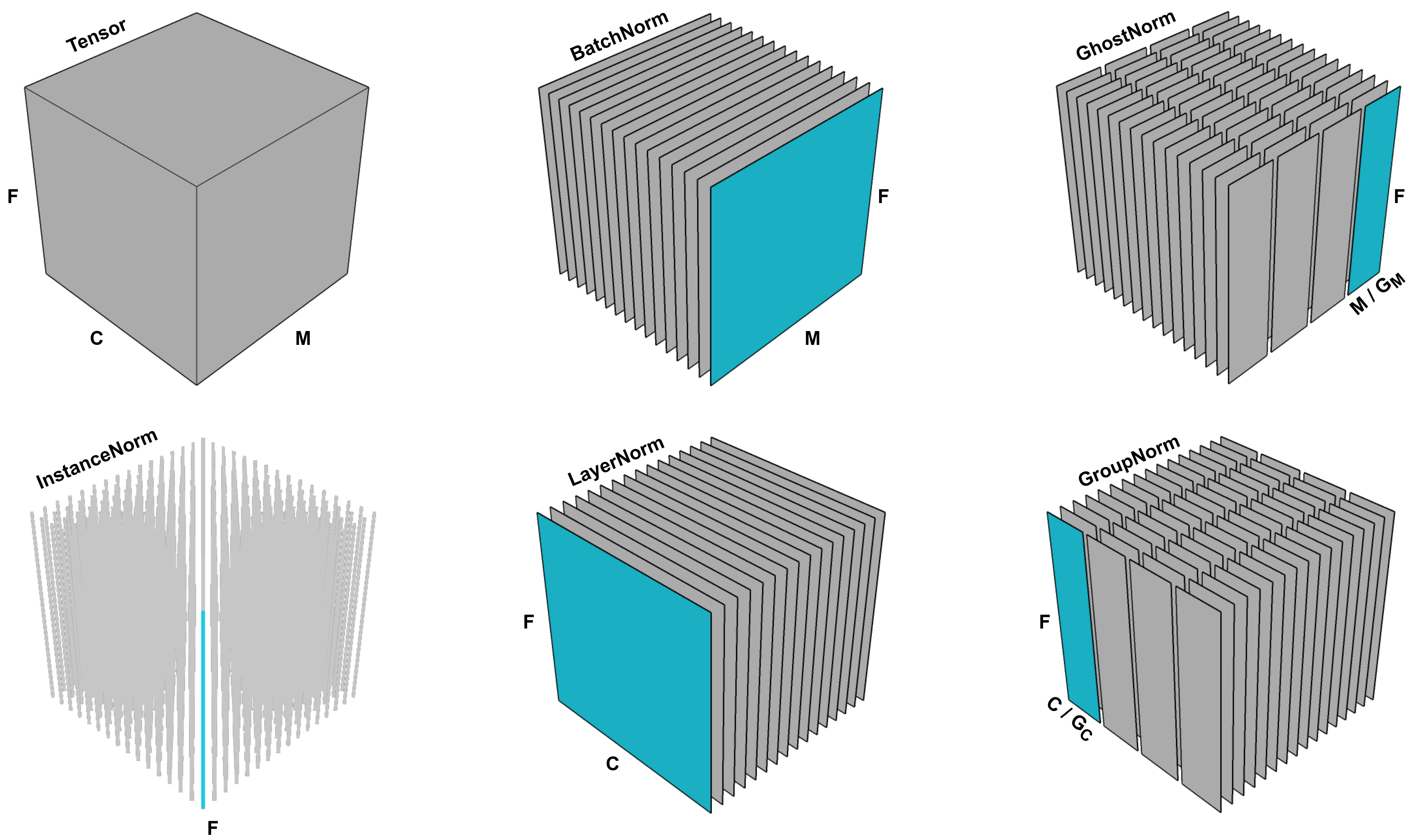
Figure 1: The input tensor is divided into a number of line (1D) or plane (2D) slices. Each normalization technique slices the input tensor differently and each slice is normalized independently of the other slices.

Given a fully-connected or convolutional neural network, the parameters of a typical layer $l$ with normalization, $Norm$, are the weights $W^{l}$ as well as the scale and shift parameters $\gamma^{l}$ and $\beta^{l}$. For brevity, we omit the $l$ superscript. Given an input tensor $X$, the activation values $A$ of layer $l$ are computed as:

$$A=g(Norm(X\odot W)\otimes\gamma+\beta)$$ (1)

where $g(\cdot)$ is the activation function, $\odot$ corresponds to either matrix multiplication or convolution for fully-connected and convolutional layers respectively, and $\otimes$ describes an element-wise multiplication.

Most normalization techniques differ in how they normalize the product ${X\odot W}$. Let the product be a tensor with ${(M,C,F)}$ dimensions where $M$ is the so-called mini–batch size, or just batch size, $C$ is the channels dimension, and $F$ is the spatial dimension.

In BatchNorm, the given tensor is normalized across the channels dimension. In particular, the mean and variance are computed across $C$ number of slices of ${(M,F)}$ dimensions (see Figure 1) which are subsequently used to normalize each channel $c\in C$ independently. In LayerNorm, statistics are computed over $M$ slices of ${(C,F)}$ dimensions, normalizing the values of each data sample $m\in M$ independently. InstanceNorm normalizes the values of the tensor over both $M$ and $C$, i.e. computes statistics across ${M\times C}$ slices of $F$ dimensions.

GroupNorm can be thought as an extension to LayerNorm wherein the $C$ dimension is divided into $G_{C}$ number of groups, i.e. ${(M,G_{C},^{C}/_{G_{C}},F)}$. Statistics are calculated over $M\times G_{C}$ slices of ${(^{C}/_{G_{C}},F)}$ dimensions. Similarly, GhostNorm can be thought as an extension to BatchNorm, wherein the $M$ dimension is divided into $G_{M}$ groups, normalizing over $C\times G_{M}$ slices of ${(^{M}/_{G_{M}},F)}$ dimensions. Both $G_{C}$ and $G_{M}$ are hyperparameters that can be tuned based on a validation set. All of the aforementioned normalization techniques are illustrated in Figure 1.

SeqNorm employs both GroupNorm and GhostNorm in a sequential manner. Initially, the input tensor is divided into ${(M,G_{C},^{C}/_{G_{C}},F)}$ dimensions, normalizing across $M\times G_{C}$ number of slices, i.e. same as GroupNorm. Then, once the $G_{C}$ and ${}^{C}/_{G_{C}}$ dimensions are collapsed back together, the input tensor is divided into ${(G_{M},^{M}/_{G_{M}},C,F)}$ dimensions for normalizing over ${C\times G_{M}}$ slices of ${(^{M}/_{G_{M}},F)}$ dimensions.

Any of the slices described above is treated as a set of values $S$ with one dimension. The mean and variance of $S$ are computed in the traditional way (see Equation 2). The values of $S$ are then normalized as shown below.

$$\mu =\frac{1}{M}\sum_{x\in S}x\text{ and }\sigma^{2}=\frac{1}{M}\sum_{x\in S}(x-\mu)^{2}$$ (2)

$$\forall x\in S\text{, }x=\frac{x-\mu}{\sqrt{\sigma^{2}+\epsilon}}$$ (3)

Once all slices are normalized, the output of the $Norm$ layer is simply the concatenation of all slices back into the initial tensor shape.

2.2 The effects of Ghost Normalization

There is only one other published work which has investigated the effectiveness of Ghost Normalization for small and medium mini-batch sizes [17]. Therein, they hypothesize that GhostNorm offers stronger regularization than BatchNorm as it computes the normalization statistics on smaller sample sizes [17]. In this section, we support that hypothesis by providing insights into a particular source of regularization, unique to GhostNorm, that stems from normalizing groups of activations during a forward pass.

Consider as an example the tuple $X$ with ${(35,39,30,4,38,26,27,19)}$ values which can be thought as an input tensor with ${(8,1,1)}$ dimensions. Given to a BatchNorm layer, the output is the normalized version $\bar{X}$ with values ${(0.7,1.1,0.3,-2.2,1.0,-0.1,-0.02,-0.8)}$. Note how although the values have changed, the ranking order of the activation values has remained the same, e.g. the 2nd value is larger than the 5th value in both $X$ (${39>38}$) and $\bar{X}$ (${1.1>1.0}$). More formally, the following holds true:

$$\begin{split}\text{Given n-tuples }X=(x_{0},x_{1},..x_{n})\text{ and }\bar{X}=(\bar{x}_{0},\bar{x}_{1},...,\bar{x}_{n})\text{,}\\ \forall i,j\in I,\bar{x}_{i}>\bar{x}_{j}\iff x_{i}>x_{j}\\ \bar{x}_{i}<\bar{x}_{j}\iff x_{i}<x_{j}\\ \bar{x}_{i}=\bar{x}_{j}\iff x_{i}=x_{j}\end{split}$$ (4)

On the other hand, given $X$ to a GhostNorm layer with $G_{M}=2$, the output $\bar{X}$ is $(0.6,0.9,0.2,-1.7,1.5,-0.2,-0.07,-1.2)$. Now, we observe that after normalization, the 2nd value has become much smaller than the 5th value in $\bar{X}$ (${0.9<1.5}$). Where BatchNorm preserves the ranking order, GhostNorm can modify the importance of each sample, and hence alter the course of optimization. Our experimental results demonstrate how GhostNorm improves upon BatchNorm, supporting the hypothesis that the above type of regularization can be beneficial to optimization. Note that for BatchNorm the condition in Equation 4 only holds true across the ${M\times F}$ dimension of the input tensor whereas for GhostNorm it cannot be guaranteed for any given dimension.

GhostNorm to BatchNorm

One can argue that the same type of regularization can be found in BatchNorm over different mini–batches, e.g. given $[35,39,30,4]$ and $[38,26,27,19]$ as two different mini–batches. However, GhostNorm introduces the above during each forward pass rather than between forward passes. Hence, it is a regularization that is embedded during learning (GhostNorm), rather than across learning (BatchNorm).

GhostNorm to GroupNorm

Despite the visual symmetry between GhostNorm and GroupNorm, there is one major difference. Grouping has been employed extensively in classical feature engineering, such as SIFT, HOG, and GIST, wherein independent normalization is often performed over these groups [14]. At a high level, GroupNorm can be thought as motivating the network to group similar features together [14]. On the other hand, that learning behaviour is not possible with GhostNorm due to random sampling, and random arrangement of data within each mini–batch. Therefore, we hypothesize that the effects of these two normalization techniques could be combined for their benefits to be accumulated. Specifically, we propose SeqNorm, a normalization technique that employs both GroupNorm and GhostNorm in a sequential manner.

2.3 Implementation

Ghost Normalization

The direct approach of implementing GhostNorm is shown in Figure 2. Although the expontential moving averages are ommited for brevity , it’s worth mentioning that they were accumulated in the same way as BatchNorm. In addition to the above direct implementation, GhostNorm can be effectively employed while using BatchNorm as the underlying normalization technique.

def GhostNorm(X, groupsM, eps=1e-05):
    """
    X: Input Tensor with (M, C, F) dimensions
    groupsM: Number of groups for the mini-batch dimension
    eps: A small value to prevent division by zero
    """
    # Split the mini-batch dimension into groups of smaller batches
    M, C, F = X.shape
    X = X.reshape(groupsM, -1, C, F)

    # Calculate statistics over dim(0) x dim(2) number
    # of slices of dim(1) x dim(3) dimension each
    mean = X.mean([1, 3], keepdim=True)
    var = X.var([1, 3], unbiased=False, keepdim=True)

    # Normalize X
    X = (X - mean) / (torch.sqrt(var + self.eps))

    # Reshape into the initial tensor shape
    X = X.reshape(M, C, F)

    return X

Figure 2: Python code for GhostNorm in PyTorch.

When the desired batch size exceeds the memory capacity of the available GPUs, practitioners often resort to the use of accumulating gradients. That is, instead of having a single forward pass with $M$ examples through the network, $n_{fp}$ number of forward passes are made with ${}^{M}/_{n_{fp}}$ examples each. Most of the time, gradients computed using a smaller number of training examples, i.e. ${}^{M}/_{n_{fp}}$, and accumulated over a number of forward passes $n_{fp}$ are identical to those computed using a single forward pass of $M$ training examples. However, it turns out that when BatchNorm is employed in the neural network, the gradients can be substantially different for the above two cases. This is a consequence of the mean and variance calculation (see Equation 2) since each forwarded smaller batch of ${}^{M}/_{n_{fp}}$ data will have a different mean and variance than if all $M$ examples were present. Accumulating gradients with BatchNorm can thus be thought as an alternative way of using GhostNorm with the number of forward passes $n_{fp}$ corresponding to the number of groups $G_{M}$. A PyTorch implementation of accumulating gradients is shown in Figure 3.

def train__for_an_epoch():
    model.train()
    model.zero_grad()
    for i, (X, y) in enumerate(train_loader):
        outputs = model(X)
        loss = loss_function(outputs, y)
        loss = loss / acc_steps
        loss.backward()
        if (i + 1) % acc_steps == 0:
            optimizer.step()
            model.zero_grad()

Figure 3: Python code for accumulating gradients in PyTorch.

Finally, the most popular implementation of GhostNorm via BatchNorm, albeit typically unintentional, comes as a consequence of using multiple GPUs. Given $n_{g}$ GPUs and $M$ training examples, $M/n_{g}$ examples are forwarded to each GPU. If the BatchNorm statistics are not synchronized across the GPUs (i.e. Synchnronized BatchNorm ref), which is often the case for image classification, then $n_{g}$ corresponds to the number of groups $G_{M}$.

A practitioner who would like to use GhostNorm should employ the implementation shown in Figure 2. Nevertheless, under the discussed circumstances, one could explore GhostNorm through the use of the other implementations.

Sequential Normalization

The implementation of SeqNorm is straightforward since it combines GroupNorm, a widely implemented normalization technique, and GhostNorm for which we have discussed three possible implementations.

3 Experiments

In this section, we first strive to take a closer look into GhostNorm by visualizing the smoothness of the loss landscape during training; a component which has been described as the primary reason behind the effectiveness of BatchNorm. Then, we evaluate the effectiveness of both GhostNorm and SeqNorm on the standard image classification datasets of CIFAR–10 and CIFAR–100. Note that in all of our experiments, the smallest ${}^{M}/_{G_{M}}$ we employ for both SeqNorm and GhostNorm is $4$. A ratio of $1$ would be undefined for normalization, whereas a ratio of $2$ results in large information corruption, i.e. all activation values are reduced to either $1$ or $-1$.

3.1 Loss landscape visualization

Implementation details

On MNIST, we train a fully-connected neural network (SimpleNet) with two fully-connected layers of $512$ and $300$ neurons. The input images are transformed to one-dimensional vectors of $784$ channels, and are normalized based on the mean and variance of the training set. The learning rate is set to $0.4$ for a batch size of $512$ on a single GPU. In addition to training SimpleNet with BatchNorm and GhostNorm, we also train a SimpleNet baseline without any normalization technique.

A residual convolutional network with $56$ layers (ResNet–56) [4] is employed for CIFAR–10. We achieve super–convergence by using the one cycle learning policy described in the work of Smith and Topin [22]. Horizontal flipping, and pad-and-crop transformations are used for data augmentation. We use a triangularly annealing learning rate schedule between $0.1$ and $3$, and down to $0.0001$ for the last few epochs. In order to train ResNet–56 without a normalization technique (baseline), we had to adjust the cyclical learning rate schedule to ($0.1$, $1$).

For both datasets, we train the networks on $50,000$ training images, and evaluate on $10,000$ testing images. For completeness, further implementation details are provided in the Appendix.

Loss landscape

We visualize the loss landscape during optimization using an approach that was described by Santurkar et al. [9]. Each time the network parameters are to be updated, we walk towards the gradient direction and compute the loss at multiple points. This enable us to visualise the smoothness of the loss landscape by observing how predictive the computed gradients are. In particular, at each step of updating the network parameters, we compute the loss at a range of learning rates, and store both the minimum and maximum loss. For MNIST, we compute the loss at $8$ learning rates $\in[0.1,0.2,0.3,...,0.8$], whereas for CIFAR–10, we do so for $4$ cyclical learning rates $\in[(0.05,1.5),(0.1,3),(0.15,4.5),(0.2,6)]$, and analogously for the baseline.

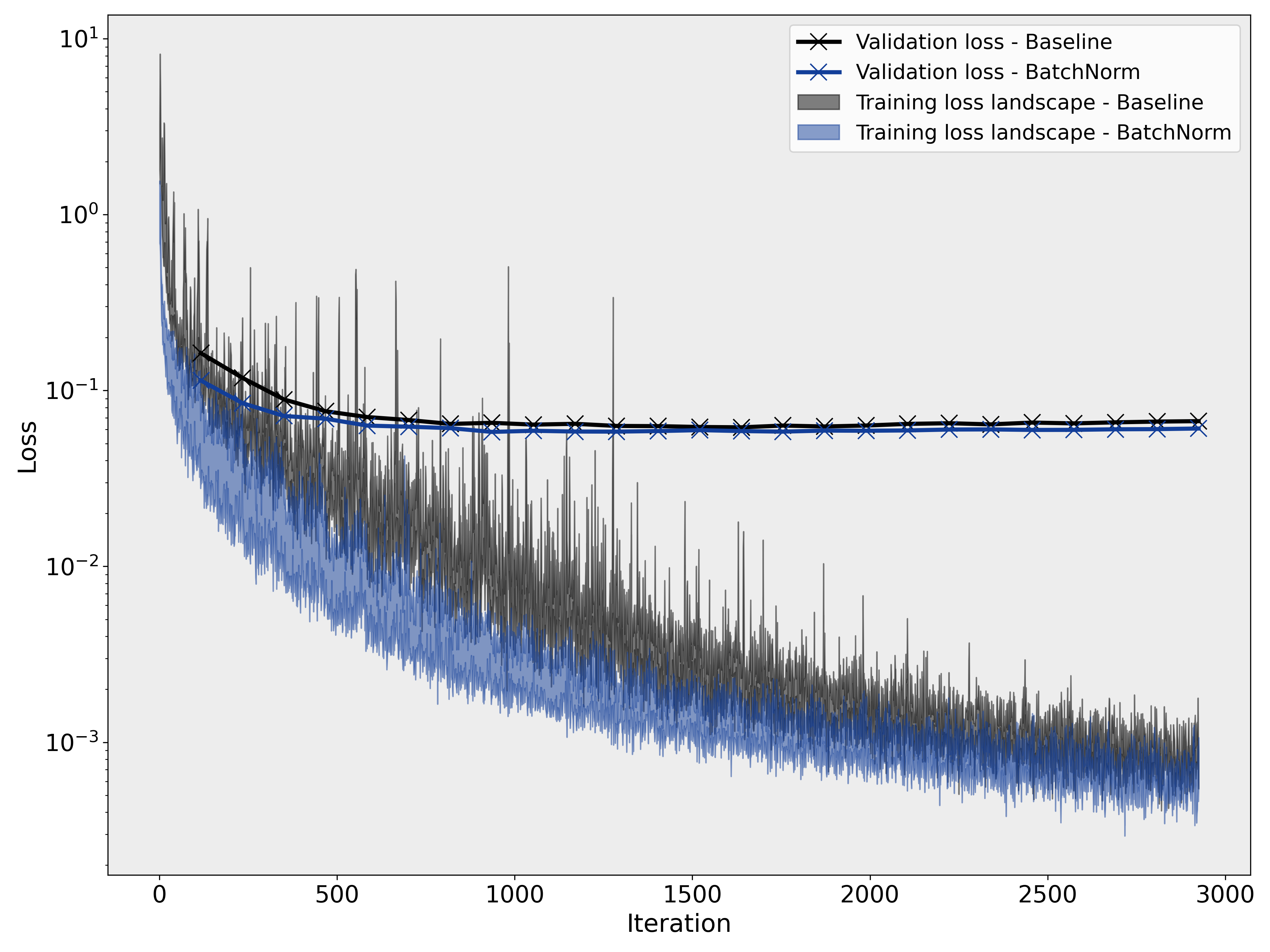
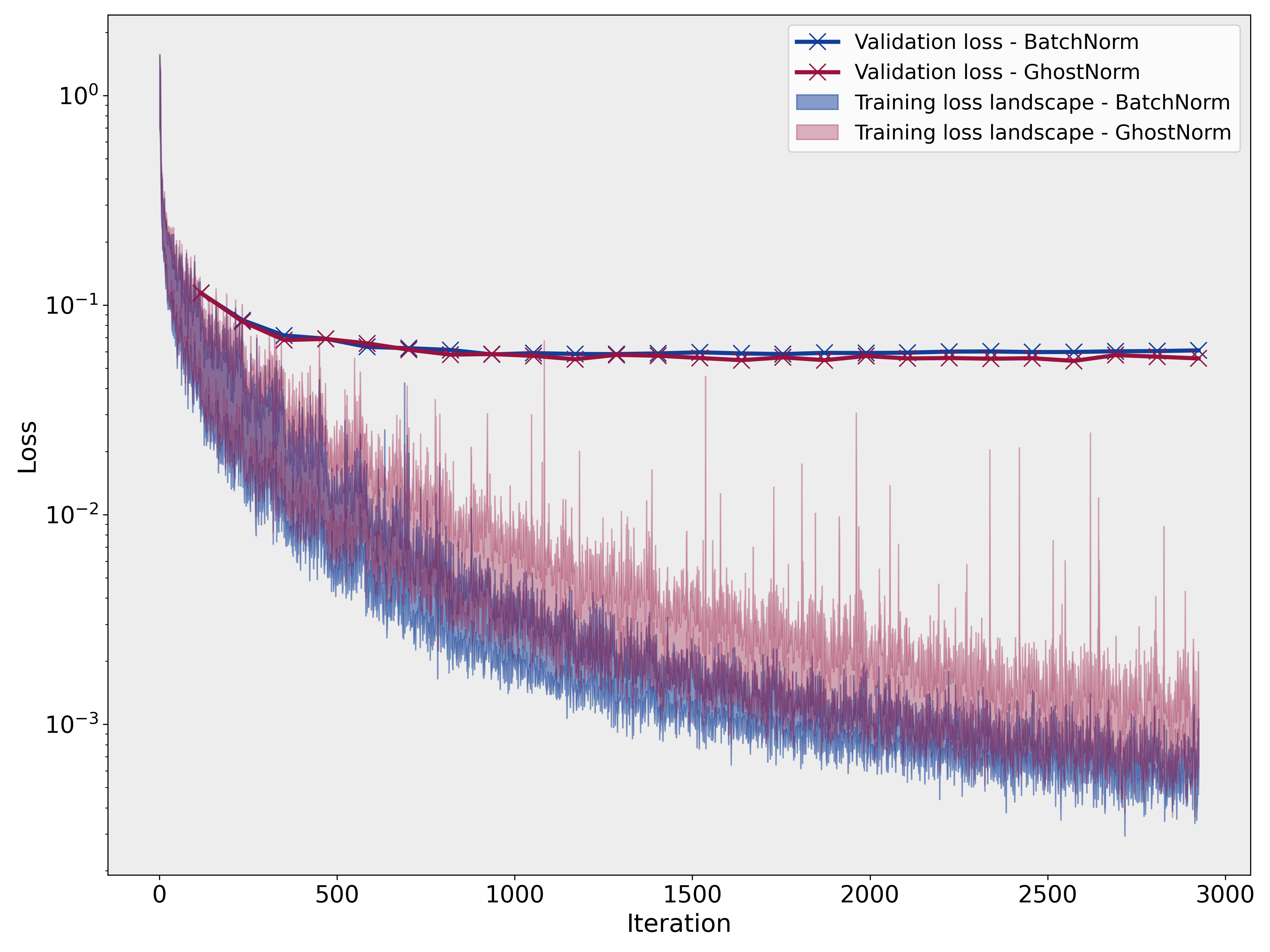
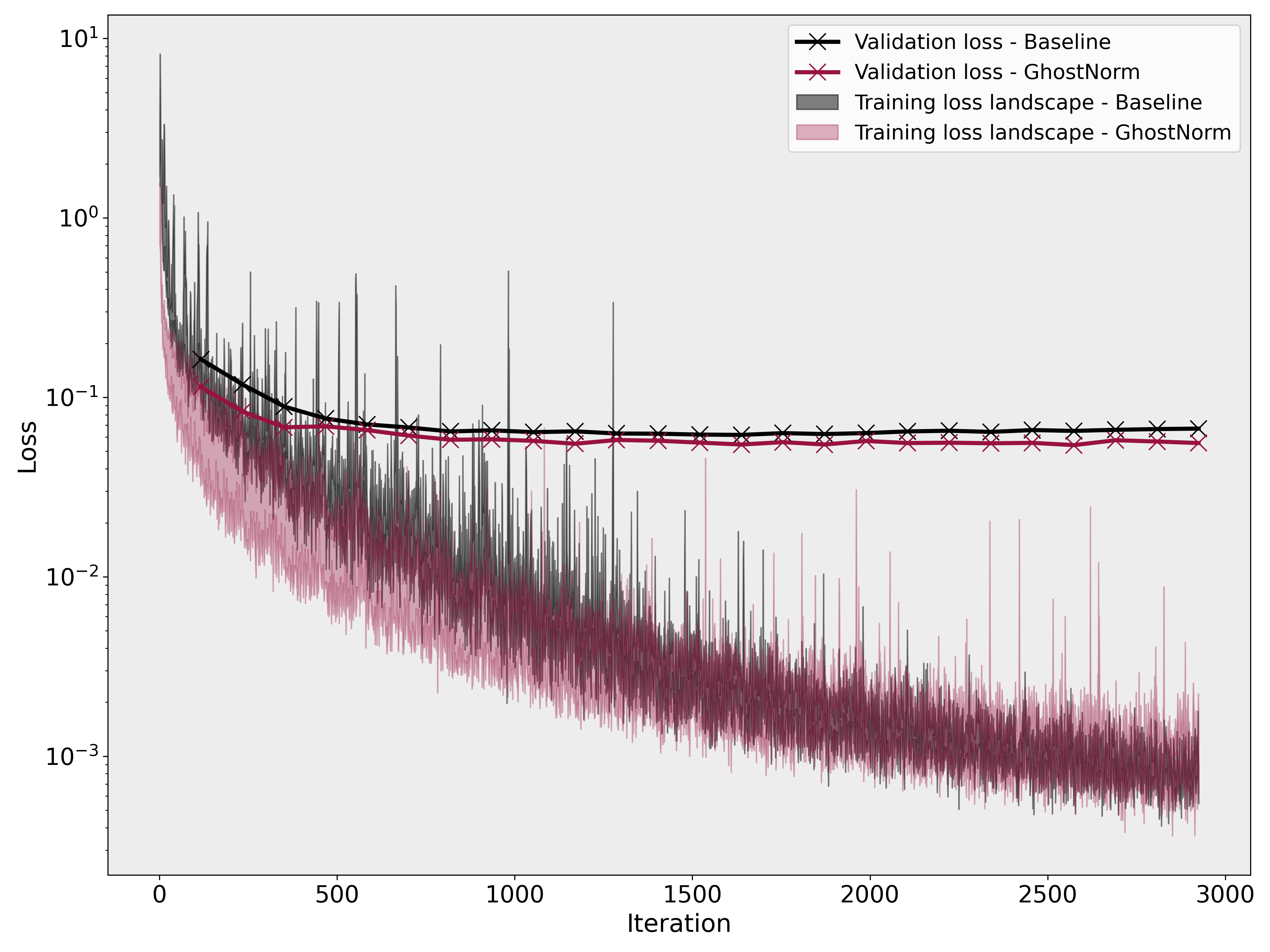
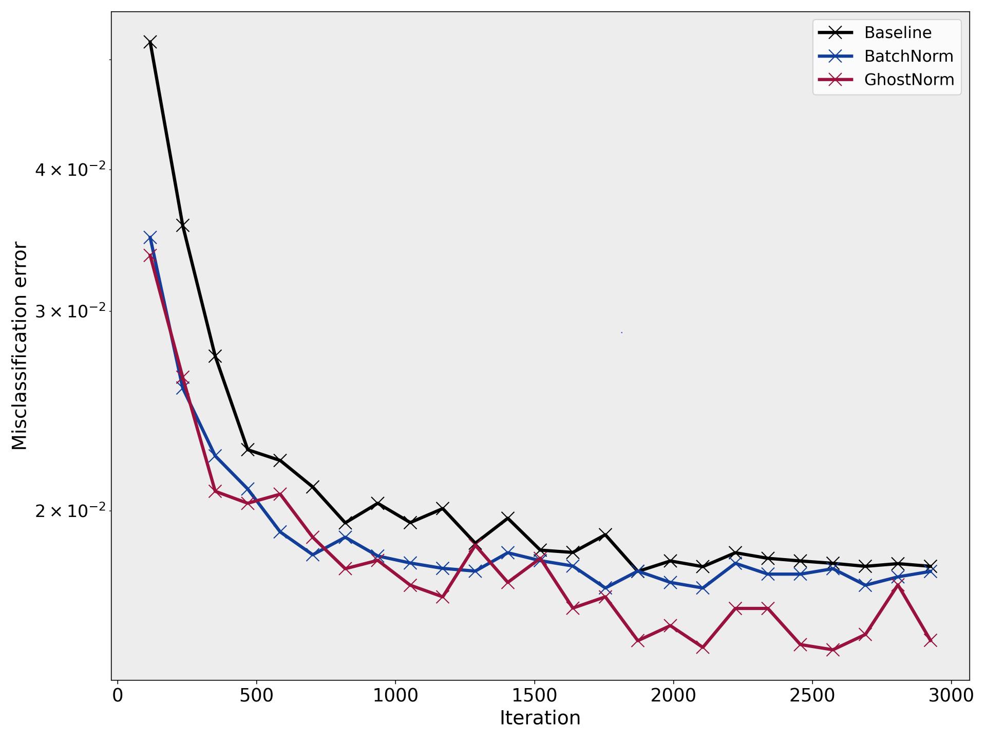
Figure 4: Comparison of the loss landscape on MNIST between BatchNorm, GhostNorm, and the baseline.

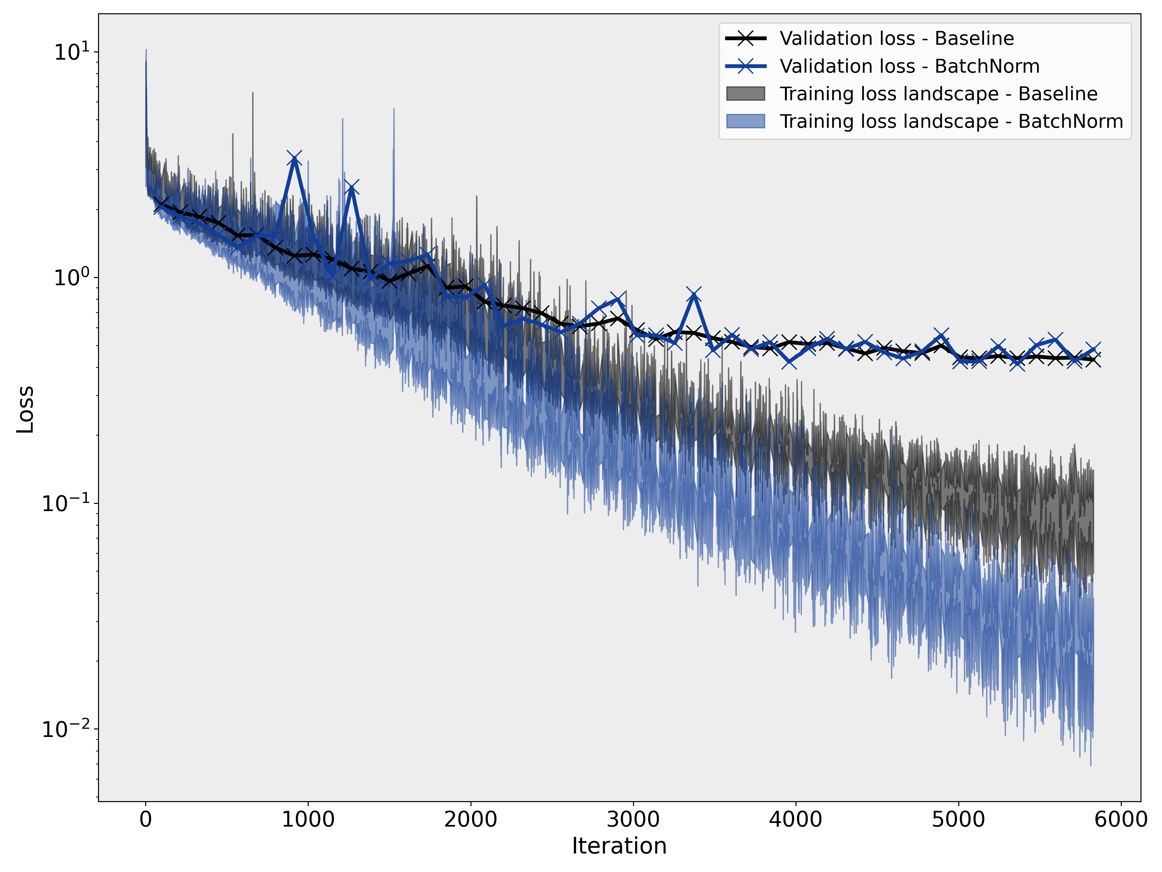
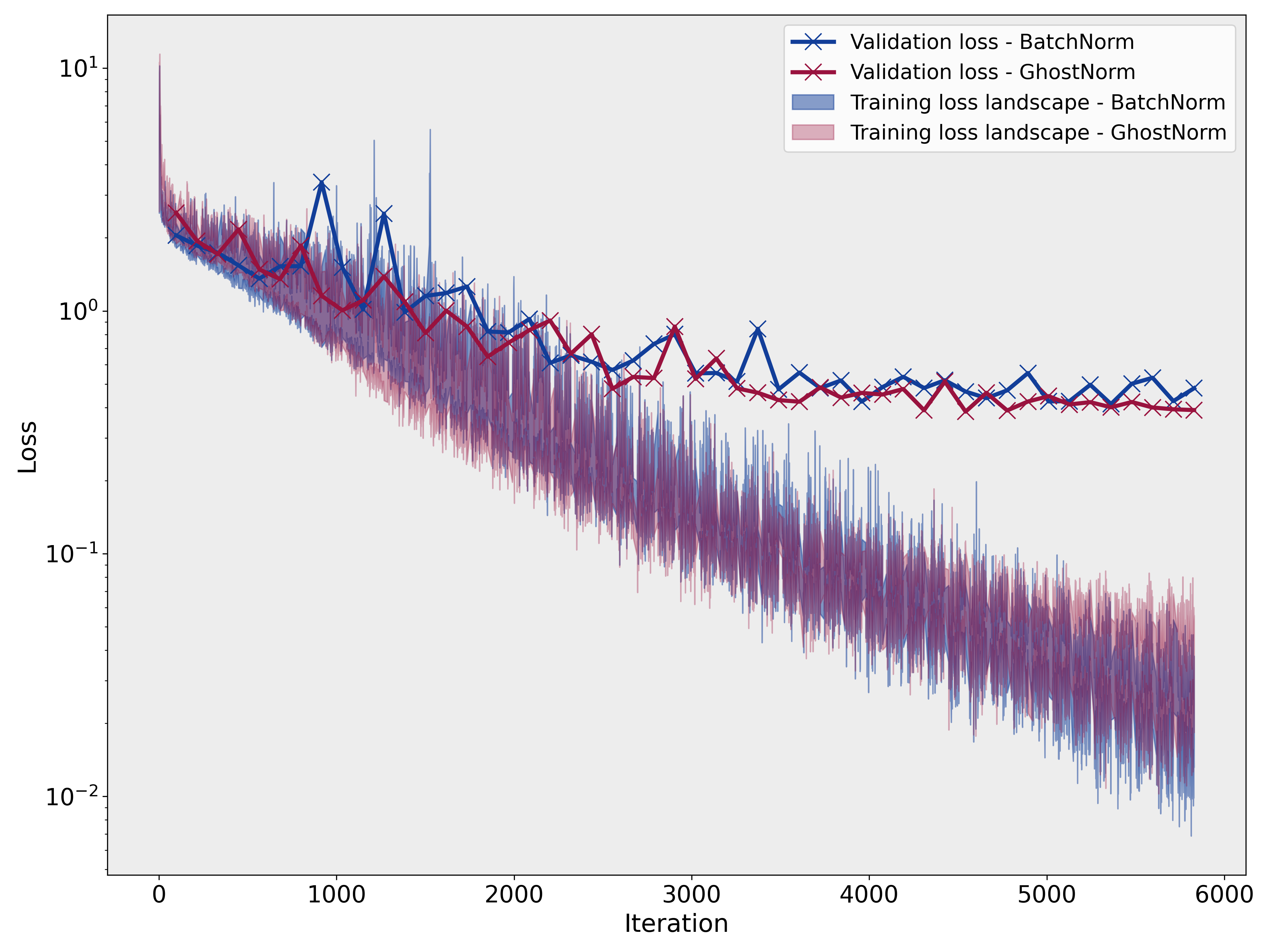
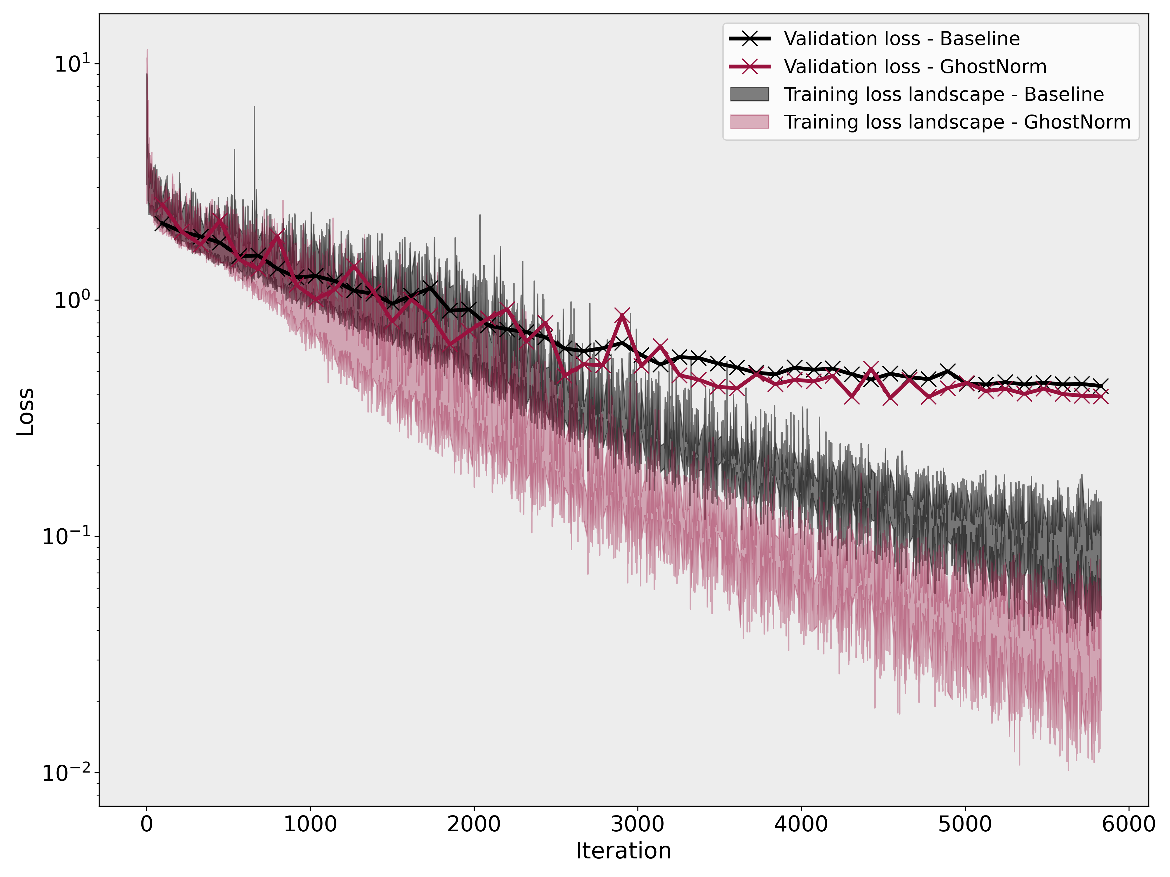
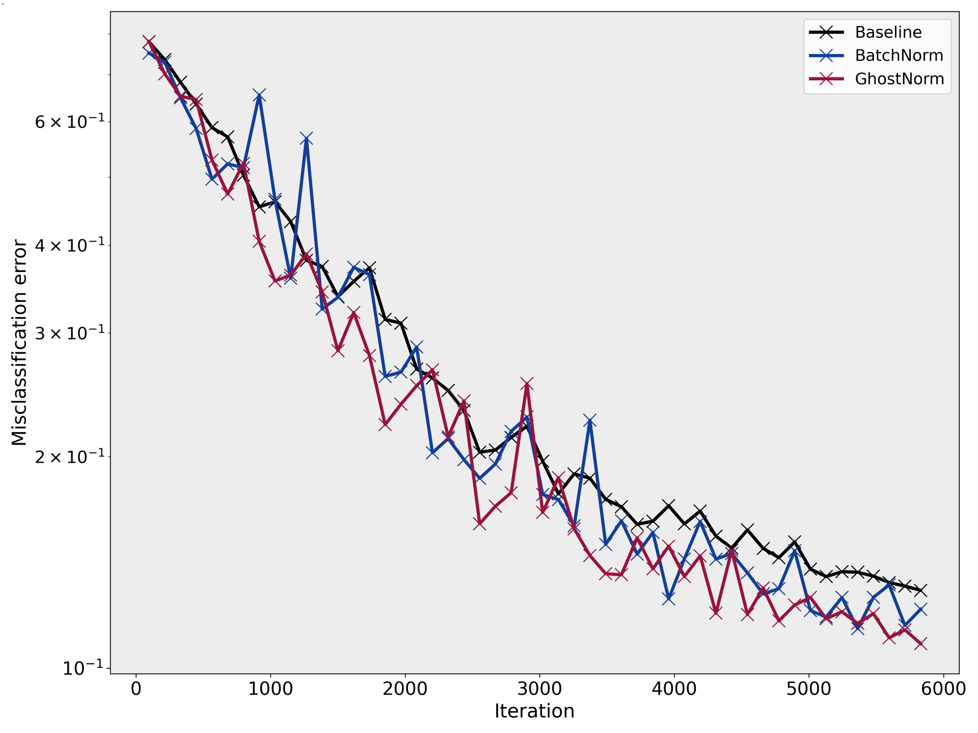
Figure 5: Comparison of the loss landscape on CIFAR–10 between BatchNorm, GhostNorm, and the baseline.

For both datasets and networks, we observe that the smoothness of the loss landscape deteriorates when GhostNorm is employed. In fact for MNIST, as seen in Figure 4, the loss landscape of GhostNorm bears closer resemblance to our baseline which did not use any normalization technique. For CIFAR–10, this is only observable towards the last epochs of training. In spite of the above observation, we have consistently witness better generalization performances with GhostNorm in almost all of our experiments, even at the extremes wherein $G_{M}$ is set to $128$, i.e. only 4 samples per group. We include further experimental results and discussion in the Appendix.

Our experimental results challenge the often established correlation between a smoother loss landscape and a better generalization performance [9, 13]. Although beyond the scope of our work, a theoretical analysis of the implications of GhostNorm when compared to BatchNorm could potentially uncover further insights into the optimization mechanisms of both normalization techniques.

3.2 Image classification

In this section, we further explore the effectiveness of both GhostNorm and SeqNorm on optimization using state-of-the-art (SOTA) methodologies for image classification. Note that the maximum $G_{C}$ is by architectural design set to $16$, i.e. the smallest layer in the network has $16$ channels.

Implementation details

For both CIFAR–10 and CIFAR–100, we employ a training set of $45,000$ images, a validation set of $5,000$ images (randomly stratified from the training set), and a testing set of $10,000$. The input data were stochastically augmented with horizontal flips, pad-and-crop as well as Cutout [23]. We use the same hyperparameter configurations as Cubuk et al. [24]. However, in order to speed up optimization, we increase the batch size from 128 to 512, and apply a warmup scheme [25] that increases the initial learning rate by four times in $5$ epochs; thereafter we use the cosine learning schedule. Based on the above experimental settings, we train Wide-ResNet models of $28$ depth and $10$ width [26] for $200$ epochs. Note that since $8$ GPUs are employed, our BatchNorm baselines are equivalent to using GhostNorm with $G_{M}=8$. Nevertheless, to avoid any confusion, we refer to it as BatchNorm. It’s worth mentioning that setting $G_{M}$ to $8$ on $8$ GPUs is equivalent to using $64$ on $1$ GPU.

CIFAR–100

Initially, we turn to CIFAR–100, and tune the hyperparameters $G_{C}$ and $G_{M}$ of SeqNorm in a grid-search fashion. The results are shown in Table 1. Both GhostNorm and SeqNorm improve upon the baseline by a large margin ($0.7\%$ and $1.7\%$ respectively). Moreover, SeqNorm surpasses the current SOTA performance on CIFAR–100, which uses a data augmentation strategy, by $0.5\%$ [24]. These results support our hypothesis that sequentially applying GhostNorm and GroupNorm can have an additive effect on improving NN optimization.

However, the grid–search approach to tuning $G_{C}$ and $G_{M}$ is rather time consuming (time complexity: $\Theta(G_{C}\times G_{M})$). Hence, we attempt to identify a less demanding hyperparameter tuning approach. The most obvious, and the one we actually adopt for the next experiment, is to sequentially tune $G_{C}$ and $G_{M}$. In particular, we find that first tuning $G_{M}$, then selecting the largest $g_{M}\in G_{M}$ for which the network performs well, and finally tuning $G_{C}$ with $g_{M}$ to be an effective approach (time complexity: $\Theta(G_{C}+G_{M})$). Note that by following this approach on CIFAR-100, we still end up with the same best SeqNorm, i.e. $G_{C}=4$ and $G_{M}=8$.

Table 1: Results on CIFAR–100 by tuning both $G_{C}$ and $G_{M}$ in a grid–search fashion. For SeqNorm, we only show the best results for each $G_{C}$. Both validation and testing performances are averaged over two different runs. Given the same mean performances between two hyperparameter configurations, the one exhibiting less performance variance was adopted.

Normalization	Validation accuracy	Testing accuracy
BatchNorm	$80.6\%$	$82.1\%$
GhostNorm ($G_{M}=2$)	$80.9\%$	-
GhostNorm ($G_{M}=4$)	$81.2\%$	-
GhostNorm ($G_{M}=8$)	$\boldsymbol{81.4\%}$	$82.8\%$
GhostNorm ($G_{M}=16$)	$80.3\%$	-
SeqNorm ($G_{C}=1$, $G_{M}=4$)	$82.3\%$	-
SeqNorm ($G_{C}=2$, $G_{M}=4$)	$82.4\%$	-
SeqNorm ($G_{C}=4$, $G_{M}=8$)	$\boldsymbol{82.5\%}$	$\boldsymbol{83.8\%}$
SeqNorm ($G_{C}=8$, $G_{M}=8$)	$82.4\%$	-
SeqNorm ($G_{C}=16$, $G_{M}=8$)	$82.3\%$	-

CIFAR–10

As the first step, we tune $G_{M}$ for GhostNorm. We observe that for ${G_{M}\in(2,4,8)}$, the network performs similarly on the validation set at $\approx 96.6\%$ accuracy. We choose $G_{M}=4$ for GhostNorm since it exhibits slightly higher accuracy at $96.7\%$.

Based on the tuning strategy described in the previous section, we adopt $G_{M}=8$ and tune $G_{C}$ for values between $1$ and $16$, inclusively. Although the network performs similarly at $\approx 96.8\%$ accuracy for ${G_{C}\in(1,8,16)}$, we choose $G_{C}=16$ as it achieves slightly higher accuracy than the rest. Using the above configuration, SeqNorm is able to match the current SOTA on the testing set [27].

Table 2: Results on CIFAR–10 based on the sequential tuning of $G_{C}$ and $G_{M}$. Both validation and testing performances are averaged over two different runs.

Normalization	Validation accuracy	Testing accuracy
BatchNorm	$96.6\%$	$97.1\%$
GhostNorm ($G_{M}=4$)	$96.7\%$	$97.3\%$
SeqNorm ($G_{C}=16$, $G_{M}=8$)	$96.8\%$	$\boldsymbol{97.4\%}$

3.3 Negative Results

A number of other approaches were adopted in conjunction with GhostNorm and SeqNorm. These preliminary experiments did not surpass the BatchNorm baseline performances on the validation sets (most often than not by a large margin), and are therefore not included in detail. Note that given a more elaborate hyperparameter tuning phase, these approaches may had otherwise succeeded.

In particular, we have also experimented with placing GhostNorm and GroupNorm in reverse order for SeqNorm (in retrospect, this could have been expected given what we describe in Section 2.2), and have also experimented with augmenting SeqNorm and GhostNorm with weight standardisation [13] as well as by computing the variance of batch statistics on the whole input tensor [ref]. Finally, for all experiments, we have attempted to tune networks with only GroupNorm [14] but the networks were either unable to converge or they achieved worse performances than the BatchNorm baselines.

4 Conclusion

It is generally believed that the cause of performance deterioration of BatchNorm with smaller batch sizes stems from it having to estimate layer statistics using smaller sample sizes [11, 14, 16]. In this work we challenged this belief by demonstrating the effectiveness of GhostNorm on a number of different networks, learning policies, and datasets. For instance, when using super–convergence on CIFAR–10, GhostNorm performs better than BatchNorm, even though the former normalizes the input activations using $4$ samples whereas the latter uses all $512$ samples. By providing novel insight on the source of regularization in GhostNorm, and by introducing a number of possible implementations, we hope to inspire further research into GhostNorm.

Moreover, based on the understanding developed while investigating GhostNorm, we introduce SeqNorm and follow up with empirical analysis. Surprisingly, SeqNorm not only surpasses the performances of BatchNorm and GhostNorm, but even challenges the current SOTA methodologies on both CIFAR–10 and CIFAR–100 that employ data augmentation strategies [24, 27]. Finally, we also describe a tuning strategy for SeqNorm that provides a faster alternative to the traditional grid–search approach.

References

- [1] S. Ioffe and C. Szegedy. Batch normalization: Accelerating deep network training by reducing internal covariate shift. In F. Bach and D. Blei, editors, International Conference on Machine Learning, volume 37, pages 448–456, July 2015.
- [2] Alex Krizhevsky, Ilya Sutskever, and Geoffrey E. Hinton. ImageNet classification with deep convolutional neural networks. Communications of the ACM, 60(6):84–90, 2017.
- [3] G. Huang, Z. Liu, and Q. K. Weinberger. Densely connected convolutional networks. CoRR, abs/1608.06993, 2016.
- [4] Kaiming He, Xiangyu Zhang, Shaoqing Ren, and Jian Sun. Deep residual learning for image recognition. 2016 IEEE Conference on Computer Vision and Pattern Recognition (CVPR), pages 770–778, 2015.
- [5] Alex Graves, Abdel-rahman Mohamed, and Geoffrey Hinton. Speech recognition with deep recurrent neural networks. In 2013 IEEE International Conference on Acoustics, Speech and Signal Processing. IEEE, 2013.
- [6] Ilya Sutskever, Oriol Vinyals, and Quoc V Le. Sequence to sequence learning with neural networks. In Z. Ghahramani, M. Welling, C. Cortes, N. D. Lawrence, and K. Q. Weinberger, editors, Advances in Neural Information Processing Systems 27, pages 3104–3112. Curran Associates, Inc., 2014.
- [7] David Silver, Aja Huang, Chris J. Maddison, Arthur Guez, Laurent Sifre, George van den Driessche, Julian Schrittwieser, Ioannis Antonoglou, Veda Panneershelvam, Marc Lanctot, Sander Dieleman, Dominik Grewe, John Nham, Nal Kalchbrenner, Ilya Sutskever, Timothy Lillicrap, Madeleine Leach, Koray Kavukcuoglu, Thore Graepel, and Demis Hassabis. Mastering the game of go with deep neural networks and tree search. Nature, 529(7587):484–489, 2016.
- [8] Volodymyr Mnih, Koray Kavukcuoglu, David Silver, Andrei A. Rusu, Joel Veness, Marc G. Bellemare, Alex Graves, Martin Riedmiller, Andreas K. Fidjeland, Georg Ostrovski, Stig Petersen, Charles Beattie, Amir Sadik, Ioannis Antonoglou, Helen King, Dharshan Kumaran, Daan Wierstra, Shane Legg, and Demis Hassabis. Human-level control through deep reinforcement learning. Nature, 518(7540):529–533, 2015.
- [9] S. Santurkar, D. Tsipras, A. Ilyas, and A. Madry. How does batch normalization help optimization? In S. Bengio, H. Wallach, H. Larochelle, K. Grauman, N. Cesa-Bianchi, and R. Garnett, editors, Advances in Neural Information Processing Systems, pages 2483–2493, 2018.
- [10] Nils Bjorck, Carla P Gomes, Bart Selman, and Kilian Q Weinberger. Understanding batch normalization. In S. Bengio, H. Wallach, H. Larochelle, K. Grauman, N. Cesa-Bianchi, and R. Garnett, editors, Advances in Neural Information Processing Systems 31, pages 7694–7705. Curran Associates, Inc., 2018.
- [11] Sergey Ioffe. Batch renormalization: Towards reducing minibatch dependence in batch-normalized models. In Proceedings of the 31st International Conference on Neural Information Processing Systems, pages 1942––1950. Curran Associates Inc., 2017.
- [12] Jimmy Lei Ba, Jamie Ryan Kiros, and Geoffrey E. Hinton. Layer Normalization. arXiv e-prints, page arXiv:1607.06450, 2016.
- [13] Siyuan Qiao, Huiyu Wang, Chenxi Liu, Wei Shen, and Alan Yuille. Weight Standardization. arXiv e-prints, page arXiv:1903.10520, 2019.
- [14] Y. Wu and K. He. Group normalization. In European Conference on Computer Vision (ECCV), 2018.
- [15] Dmitry Ulyanov, Andrea Vedaldi, and Victor Lempitsky. Instance Normalization: The Missing Ingredient for Fast Stylization. arXiv e-prints, page arXiv:1607.08022, July 2016.
- [16] Junjie Yan, Ruosi Wan, Xiangyu Zhang, Wei Zhang, Yichen Wei, and Jian Sun. Towards stabilizing batch statistics in backward propagation of batch normalization. In International Conference on Learning Representations, 2020.
- [17] Cecilia Summers and Michael J. Dinneen. Four things everyone should know to improve batch normalization. In International Conference on Learning Representations, 2020.
- [18] Elad Hoffer, Itay Hubara, and Daniel Soudry. Train longer, generalize better: Closing the generalization gap in large batch training of neural networks. In Proceedings of the 31st International Conference on Neural Information Processing Systems, NIPS’17, pages 1729––1739. Curran Associates Inc., 2017.
- [19] Ping Luo, Jiamin Ren, Zhanglin Peng, Ruimao Zhang, and Jingyu Li. Differentiable learning-to-normalize via switchable normalization. In International Conference on Learning Representations, 2019.
- [20] Jonas Kohler, Hadi Daneshmand, Aurelien Lucchi, Thomas Hofmann, Ming Zhou, and Klaus Neymeyr. Exponential convergence rates for batch normalization: The power of length-direction decoupling in non-convex optimization. In Kamalika Chaudhuri and Masashi Sugiyama, editors, Proceedings of Machine Learning Research, volume 89 of Proceedings of Machine Learning Research, pages 806–815. PMLR, 16–18 Apr 2019.
- [21] Chunjie Luo, Jianfeng Zhan, Lei Wang, and Wanling Gao. Extended Batch Normalization. arXiv e-prints, page arXiv:2003.05569, March 2020.
- [22] Leslie N. Smith and Nicholay Topin. Super-Convergence: Very Fast Training of Neural Networks Using Large Learning Rates. arXiv e-prints, page arXiv:1708.07120, August 2017.
- [23] Terrance DeVries and Graham W. Taylor. Improved Regularization of Convolutional Neural Networks with Cutout. arXiv e-prints, page arXiv:1708.04552, 2017.
- [24] Ekin D. Cubuk, Barret Zoph, Jonathon Shlens, and Quoc V. Le. RandAugment: Practical automated data augmentation with a reduced search space. arXiv e-prints, page arXiv:1909.13719, 2019.
- [25] Priya Goyal, Piotr Dollár, Ross Girshick, Pieter Noordhuis, Lukasz Wesolowski, Aapo Kyrola, Andrew Tulloch, Yangqing Jia, and Kaiming He. Accurate, Large Minibatch SGD: Training ImageNet in 1 Hour. arXiv e-prints, page arXiv:1706.02677, 2017.
- [26] S. Zagoruyko and N. Komodakis. Wide residual networks. CoRR, abs/1605.07146, 2016.
- [27] Ekin D. Cubuk, Barret Zoph, Dandelion Mane, Vijay Vasudevan, and Quoc V. Le. Autoaugment: Learning augmentation strategies from data. In The IEEE Conference on Computer Vision and Pattern Recognition (CVPR), June 2019.