Optical spin initialization of spin-$\frac{3}{2}$ silicon vacancy centers in 6H-SiC at room temperature

Abstract

Silicon vacancies in silicon carbide have been proposed as an alternative to nitrogen vacancy centers in diamonds for spintronics and quantum technologies. An important precondition for these applications is the initialization of the qubits into a specific quantum state. In this work, we study the optical alignment of the spin 3/2 negatively charged silicon vacancy in 6H-SiC. Using time-resolved optically detected magnetic resonance, we coherently control the silicon vacancy spin ensemble and measure Rabi frequencies, spin-spin and spin-lattice relaxation times of all three transitions. Then to study the optical initialization process of the silicon vacancy spin ensemble, the vacancy spin ensemble is prepared in different ground states and optically excited. We describe a simple rate equation model that can explain the observed behaviour and determine the relevant rate constants.

I Introduction

Silicon carbide (SiC) exists in many polytypes and hosts many interesting vacancy centers, which have been shown to be useful for applications in quantum technologies like sensing Falk et al. (2013); Widmann et al. (2015); Christle et al. (2015); Baranov et al. (2013); Anisimov et al. (2018, 2016); Koehl et al. (2011).Based on their spin in the ground state, these vacancy centers can be divided into two categories: $S=1$ or $S=3/2$ Riedel et al. (2012); Soykal et al. (2016). Neutral divacancies, consisting of neighboring C and Si vacancies, have spin 1. Four different types of divacancies in 4H-SiC have been studied using optical and microwave techniques Koehl et al. (2011) similar to those used with nitrogen-vacancy qubits in diamond Doherty et al. (2013); Suter and Jelezko (2017); Suter (2020). They can be efficiently polarized by optical irradiation and their polarization can be transferred to ²⁹Si nuclear spins, which are strongly coupled to divacancies in 4H- and 6H-SiC Falk et al. (2015). Coherent control of divacancy spins in 4H-SiC can be achieved even at high temperature up to 600 K Yan et al. (2018). The spins of neutral divacancies in SiC can sensitively detect both strain and electric fields Falk et al. (2014), with higher sensitivity than NV centers in diamond Falk et al. (2013, 2014).

Another type of vacancies consists of missing silicon atoms, i.e., silicon vacancies. If they capture an additional electron, they become negatively charged silicon vacancies (V${}_{Si}^{-}$) and have spin 3/2 Riedel et al. (2012); Soykal et al. (2016); Soltamov et al. (2012); Baranov et al. (2013); Biktagirov et al. (2018). Several individually addressable silicon-vacancies have been identified in different SiC polytypes. For example, the 6H-SiC hosts one hexagonal site $h$ and two cubic sites ($k_{1}$ and $k_{2}$). V${}_{Si}^{-}$ at $k_{1}$ and $k_{2}$ are called V₁ and V₃, respectively, whereas V${}_{Si}^{-}$ at the hexagonal sites $h$ are called V₂ Sörman et al. (2000); Biktagirov et al. (2018). Recently, it has been shown that $V_{Si}^{-}$ at hexagonal lattice sites $h$ corresponds to V₁ and V${}_{Si}^{-}$ at cubic lattice sites $k_{1}$ and $k_{2}$ are V₃ and V₂, respectively Davidsson et al. (2019). These negatively charged vacancies have zero phonon lines (ZPL) at 865 nm (V$1$), 887 nm (V$2$), and 908 nm (V$3$) Sörman et al. (2000); Biktagirov et al. (2018); Singh et al. (2020). Optically induced alignment of the ground-state spin sublevels of the V${}_{Si}^{-}$ in 4H- and 6H-SiC has been demonstrated at room temperature Soltamov et al. (2012). Coherent control of a single silicon-vacancy spin and long spin coherence times have been reported Widmann et al. (2015). V${}_{Si}^{-}$ are relatively immune to electron-phonon interactions and do not exhibit fast spin dephasing (spin coherence time $T_{2}=0.85$ ms) Nagy et al. (2019). Using a moderate magnetic field in combination with dynamic decoupling, the spin coherence of the V${}_{Si}^{-}$ spin ensemble in 4H-SiC with natural isotopic abundance can be preserved over an unexpectedly long time of >20 ms Simin et al. (2017). Quantum microwave emitters based on V${}_{Si}^{-}$ in SiC at room temperature Kraus et al. (2014) can be enhanced via fabrication of Schottky barrier diodes and can be modulated by almost 50% by an external bias voltage Bathen et al. (2019). Using all four levels, V${}_{Si}^{-}$ can be used for absolute dc magnetometry  Soltamov et al. (2019).

In our previous work, we studied the temperature-dependent photoluminescence, optically detected magnetic resonance (ODMR), and the relaxation times of the V${}_{Si}^{-}$ spin ensemble in 6H-SiC at room temperature Singh et al. (2020).

In this work, we focus on the optical spin initialization of the V₁/V₃ in 6H-SiC, the spin relaxation and the dynamics of the intersystem-crossing. Section II gives details of the optical pumping process. Section III explains the experimental setup for continuous-wave (cw)- double-resonance and pulsed ODMR measurements. Section IV describes the measurements of the spin-lattice relaxation rates. Section V describes the dynamics of the optical spin alignment. Section VI contains a brief discussion and concluding remarks.

II System

The 6H-SiC sample we used is isotopically enriched in ²⁸Si and ¹³C Singh et al. (2020). The presence of 4.7 % ¹³C reduces the coherence time of the vacancy spin centers Yang et al. (2014). Details of the sample preparation are given in Appendix A. In our previous work Singh et al. (2020), PL spectra revealed the negative charged vacancies’ zero phonon lines (ZPL) at 865 nm (V$1$), 887 nm (V$2$), and 908 nm (V$3$).

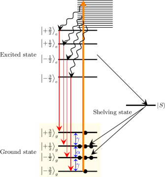
Figure 1: The ground, excited, and shelving states of the 6H-SiC V₁/V₃ form V${}_{Si}^{-}$ are shown in this energy-level diagram. Red arrows indicate radiative transitions. An orange arrow for the non-resonant laser excitation. Black arrow shows the spin-dependent non-radiative transitions. The states $|.\rangle_{g}$ represent ground states, $|.\rangle_{e}$ the excited states and $|S\rangle$ the shelving states.

The negatively charged V₁/V₃ type silicon vacancy center in 6H-SiC has spin $S$ = 3/2 Riedel et al. (2012); Soykal et al. (2016). Figure 1 is the energy-level scheme in an external magnetic field. The states $|.\rangle_{g}$ and $|.\rangle_{e}$ the electronically ground and excited states repectively Kraus et al. (2014); Biktagirov et al. (2018); Baranov et al. (2011); Fuchs et al. (2015). The shelving state $|S\rangle$ is an $S=1/2$ state. This is essential for the optical pumping process Baranov et al. (2011) during which it gets populated by intersystem crossing (ISC).

The ground state spin Hamiltonian of the V₁/V₃ type defect is

$$\mathcal{H}=D(S_{z}^{2}-\frac{5}{4}\hat{I})+g\mu_{B}\vec{B}\cdot\text{$\vec{S}$},$$ (1)

where $g=2.0$ (electron $g$-factor), $2D=-28$ MHz (the zero field splitting) Biktagirov et al. (2018); Singh et al. (2020), $\mu_{B}$ is the Bohr magneton, $\hat{I}$ the unit operator, $\vec{B}$ is the magnetic field strength, and $\vec{S}$ is the four level electron spin operators. We choose $z$-axis of our coordinate system such that it is parallel to the $c$-axis of the crystal (C₃ symmetry axis).

At ambient temperature, almost all four ground states have equal populations when the vacancy spin system is in thermal equilibrium in the absence of optical pumping. The populations of the spin states $|\pm\frac{1}{2}\rangle_{g}$ become large compared to those of $|\pm\frac{3}{2}\rangle_{g}$, when the system is excited with a laser light, as shown schematically in Fig. 1 Baranov et al. (2011); Kraus et al. (2014). With the laser light illumination, the population of ground state goes to the excited states and with the spontaneous emission it come back to the ground states. During the excited state lifetime, which is $\sim$10 ns in the 6H polytype, estimated from the linewidth of the excited state level anti-crossing (LAC) Astakhov et al. (2016) and $\sim$7.8 ns  in 4H Fuchs et al. (2015); Hain et al. (2014). Although, the spin system can go through intersystem-crossing (ISC) to the shelving states $|S\rangle$ Baranov et al. (2011). The measured time constant from the excited state to $|S\rangle$ is $\sim$16.8 ns for V${}_{Si}^{-}$ in 4H Fuchs et al. (2015). The system then returns to its initial state, with a preference for the states. $|\pm\frac{1}{2}\rangle$ is preferable to $|\pm\frac{3}{2}\rangle$, with a time constant 150 ns for V${}_{Si}^{-}$ in 4H Fuchs et al. (2015); Riedel et al. (2012); Biktagirov et al. (2018); Soltamov et al. (2019). The exact rates from the excited state to $|S\rangle$ and from $|S\rangle$ to the ground state have not been measured yet for V${}_{Si}^{-}$ in the 6H-SiC polytype, but they should be close to those in the 4H-SiC polytype.

If the spins are not in thermal equilibrium and pumping stops, they relax back to the thermal equilibrium state by spin-lattice relaxation, as shown by the blue arrows in Fig. 1. Here, $\gamma$ and $\alpha$ are the spin-lattice relaxation rates of the $|\pm\frac{3}{2}\rangle$$\longleftrightarrow$$|\pm\frac{1}{2}\rangle$ and $|+\frac{1}{2}\rangle$$\longleftrightarrow$$|-\frac{1}{2}\rangle$ transitions.

III Optically detected magnetic resonance

The ODMR technique is similar to the conventional electron spin resonance (ESR) technique except for the additional optical pumping and the detection part. In the ODMR technique, instead of measuring absorbed microwave or radio frequency (RF) power, an optical signal is detected, which may be photoluminescence (PL) or a transmitted or reflected laser beam Chen (2003); Depinna and Cavenett (1982); Langof et al. (2002); Suter (2020). The detailed description of the ODMR setup is given in Appendix B.

III.1 Continuous-wave ODMR

Figure 2(b) depicts the ODMR signal measured in the absence of a magnetic field by sweeping the direct digital synthesizer (DDS) frequency as the black curve. Two peaks at 28 MHz and 128 MHz with opposite signs are recorded. The PL signal is increase at 28 MHz RF and decrease at 128 MHz.

Figure 2: (a) Energy levels of the V₁/V₃ vacancy in a magnetic field $B$ $\parallel$ $c$-axis. (b) ODMR signals vs. frequency. The black curve is the ODMR signal measured in the absence of a magnetic field, the red curve is the ODMR signal in the 3.7 mT magnetic field, and the orange curve is the ODMR with additional 77 MHz RF in the 3.7 mT magnetic field.

Fig. 2(a) shows energy levels of V₁/V₃ with magnetic field $B$ applied $parallel$ $c$-axis, calculated using the given Hamiltonian in Eq. (1).

The transition $|+3/2\rangle\leftrightarrow|+1/2\rangle$, $|+1/2\rangle\leftrightarrow|-1/2\rangle$ and $|-3/2\rangle\leftrightarrow|-1/2\rangle$, are represented by arrows labeled with $\nu{}_{1}$, $\nu{}_{2}$ and $\nu{}_{3}$, respectively. With classical ODMR experiments, only two of the three allowed transitions in the spin-3/2 system are observable, since the $\pm 1/2$ states have equal populations.

The ODMR signal recorded in a 3.7 mT magnetic field is plotted as the red curve in Fig. 2(b). The peak at 77 MHz corresponds to the $\nu_{1}$ transition, and the peak at 129 MHz corresponds to the $\nu_{3}$ transition. The negative peak around the 30 MHz is due the V₂ type V${}_{Si}^{-}$. Due to the equal populations of the $|\pm 1/2\rangle$ levels, no peak is visible at the frequency of the $\nu_{2}$ transition. To observe this transition, we added a second RF source to the setup, using it to selectively change the populations. For these experiments, the pump frequency was applied at frequency $\nu_{1}$ while the second device was scanned. The output signals of both sources were combined with an RF combiner, amplified and sent to the RF coils. The inset of Fig. 2(b) shows the modification of the populations by the pumping. Sweeping the second DDS, we recorded the ODMR signal plotted as the orange curve in Fig. 2(b) where the $\nu_{2}$ transition appears at 101 MHz. At room temperature, the PL from various types of vacancies cannot be separated Singh et al. (2020). As a result, the calculated PL contains contributions from other centers that are independent of magnetic resonance, resulting in a relatively small contrast.Further, the ODMR contrast of V${}_{Si}^{-}$ depends on the ratio of these spontaneous and non-radiative transitions. So, it would be interesting to find alternate laser excitation pathways that provide higher ODMR contrast as well as spin polarization.

III.2 Pulsed ODMR

To measure rates and time constants, we used time-resolved ODMR. To initialize the V${}_{Si}^{-}$ in all experiments, a laser pulse with a power of 100 mW and a length of 300 $mu$s was used, i.e., populating the states $|\pm\frac{1}{2}\rangle$ more than the states $|\pm\frac{3}{2}\rangle$. Following the polarization of the spin system, the system was subjected to a series of RF pulses, as detailed below. We applied a second laser pulse of duration 4 $\mu$s and integrated the PL collected during the pulse to read the state of the spin system. To discard unnecessary background signals, the signal was summed 400 times and subtracted it from a reference experiment’s 400 times summed signal. This procedure was carried out 20 times in total, with the average being taken each time Singh et al. (2020).

In the following, we assume that the population $\rho_{kk}$ of the $\pm 3/2$ spin levels contributes a fraction $\Delta$ more to the PL signal than the $\pm 1/2$ spin levels Nagy et al. (2019); Carter et al. (2015). The total PL signal $S$, measured with the second laser pulse, is then

$$S=S_{+\frac{3}{2}}+S_{+\frac{1}{2}}+S_{-\frac{1}{2}}+S_{-\frac{3}{2}}$$ (2)

with the contributions

$$S_{+\frac{3}{2}} = (S_{0}+\Delta)\rho_{11}$$

$$S_{+\frac{1}{2}} = (S_{0}-\Delta)\rho_{22}$$

$$S_{-\frac{1}{2}} = (S_{0}-\Delta)\rho_{33}$$

$$S_{-\frac{3}{2}} = (S_{0}+\Delta)\rho_{44}$$

from the populations of the different levels, where $S_{0}$ is the average signal contribution from each level. Taking into account that the sum of the populations is =1, this can be further simplified to

$$S=4S_{0}+\Delta(\rho_{11}-\rho_{22}-\rho_{33}+\rho_{44}).$$ (3)

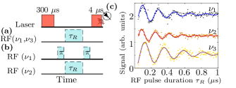
Figure 3: Pulse sequence for measuring Rabi oscillations of (a) $\nu_{1}$ and $\nu_{3}$ transitions; (b) $\nu_{2}$ transition. The laser and RF pulses are represented by the red and light green boxes. (c) Experimental Rabi oscillations. The $y$-axis represents the PL signal change, while the $x$ axis represents the RF pulse length.

We measured Rabi oscillations for the $\nu_{1}$ and $\nu_{3}$ transitions of the V$1$/ V$3$ type V${}_{Si}^{-}$, using the pulse sequence scheme given in Fig. 3(a). An RF pulse of $\tau_{R}$ duration was applied after the polarization laser pulse. for the reference signal same experiment is repeated without RF Pulse.

Rabi oscillations for the $\nu_{2}$ transition were measured using the pulse sequence shown in Fig. 3 (b). Two $\pi$ pulses with frequency $\nu_{1}$ were applied, and between them an RF pulse with frequency $\nu_{2}$ and variable duration $\tau_{R}$. The reference signal was obtained from an experiment without the RF pulses. Figure 3 (c) depicts the experimentally obtained data for the transitions at $\nu_{1}$, $\nu_{2}$ and $\nu_{3}$. The following function was used to fit the experimental data

$$S_{RF}(\tau_{R})-S_{0}(\tau_{R})=A+B\text{~}cos(2\pi f_{R}\tau_{R}-\phi)e^{-\tau_{R}/T_{2}^{\text{$R$}}},$$ (4)

here S_RF($\tau_{R}$) is the PL signal measured with a duration $\tau_{R}$ , and S₀($\tau_{R}$) is the reference signal measured with a delay $\tau_{R}$ and without the RF pulse. The Rabi frequencies obtained with 20 W RF power and the measured dephasing times $T_{2}^{R}$ are given in Table 1. A plot of the Rabi frequencies versus the square root of the RF power and a plot of the dephasing times versus the Rabi frequencies of the transitions is given in Appendix C.

Transition frequency	$f_{R}$ (MHz)	$T_{2}^{R}$ (ns)
$\nu_{1}$ (77 MHz)	$5.26\pm 0.05$	$299\pm 30$
$\nu_{2}$ (101 MHz)	$6.14\pm 0.05$	$285\pm 27$
$\nu_{3}$ (129 MHz)	$4.29\pm 0.03$	$381\pm 29$

Table 1: Parameters of the Rabi oscillations for the different transitions of V₁/ V₃ type V${}_{Si}^{-}$.

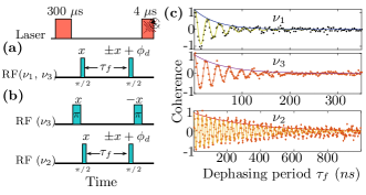
Figure 4: Pulse sequence to measure the free induction decay of (a) $\nu_{1}$ and $\nu_{3}$ transitions; (b) $\nu_{2}$ transition. (c) FID signals measured at the transitions $\nu_{1}$, $\nu_{3}$ and $\nu_{2}$. The oscillation frequency is given by the detuning frequency of the pulse sequence, which is 40 MHz in all 3 cases.

Next, we performed free induction decay (FID) and spin-echo measurements to measure the decay of coherence of all three transitions at room temperature and in the 3.7 mT magnetic field. FID measurement include coherence decay due to homogeneous and inhomogeneous interactions. For FID measurements, we used the Ramsey scheme  Ramsey (1950), in which the coherence was transformed into a population by the second $\pi/2$ RF pulse, after that, during the final laser pulse, the PL signal was read out. Figure 4 (a) shows the pulse sequence scheme for FID measurements of transitions $\nu_{1}$ and $\nu_{3}$ : First the system was initialized by the laser pulse, the coherence was created with the first $\pi/2$ RF pulse of frequency $\nu_{1}$($\nu_{3}$),then allowed to evolve for a time $\tau_{f}$ and then a $\pi/2$ RF pulse with phase $\phi_{d}=f_{det}\tau_{f}$ was applied before the readout laser pulse. We took the difference between two experiments, in which only difference is the second $\pi/2$ RF pulses have phases $\phi_{d}$ in one experiment and $\pi+\phi_{d}$ in the other which suppress unwanted background signals Singh et al. (2020). The pulse sequence for the measurement of the FID at $\nu_{2}$ is shown in Figure 4(b). It uses two additional $\pi$ pulses at frequency $\nu_{3}$ with a phase difference of $\pi$, and 2 $\pi/2$ pulses at frequency $\nu_{2}$. Figure 4 (c) shows the FIDs measured for $\nu_{1}$, $\nu_{3}$ and $\nu_{2}$ respectively with detuning of $f_{det}$= 40 MHz, along with a fit function

$$S^{FID}_{x+\phi_{d}}-S^{FID}_{-x+\phi_{d}}=A\>cos(2\pi f_{det}\tau_{f}+\phi)e^{-\tau_{f}/T_{2}^{*}}$$ (5)

where $S^{FID}_{x}+\phi_{d}(\tau_{f})$ and $S^{FID}_{-x}+\phi_{d}(\tau_{f})$ are the averaged PL signals measured with the second $\pi/2$ RF pulse with phase $\pm x+\phi_{d}$. The decay time $T_{2}^{*}$ is $46\pm 6$ ns for transition $\nu_{1}$, $333\pm 40$ ns for transition $\nu_{2}$ and $66\pm 8$ ns for transition $\nu_{3}$. The longer dephasing time for the transition $\nu_{2}$ ($+1/2\leftrightarrow-1/2$) is expected as it is not affected by the zero-field splitting Eickhoff and Suter (2004); Soltamov et al. (2019) and therefore less affected by inhomogeneous broadening than the two transitions $\nu_{1}$ and $\nu_{3}$.

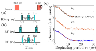
Figure 5: Pulse sequence for spin-echo experiments at (a) $\nu_{1}$ and $\nu_{3}$ transitions and (b) $\nu_{2}$ transition. (c) Spin-echo signals measured at the transitions $\nu_{1}$, $\nu_{2}$, and $\nu_{3}$.

To measure the coherence decay due to the homogeneous interactions, we performed the spin-echo experiment (Hahn echo) Hahn (1950). Figure 5(a) shows the pulse sequence for the spin-echo measurement of transitions $\nu_{1}$ and $\nu_{3}$, and Fig. 5(b) shows for transition $\nu_{2}$. The pulse sequences used to measure the spin-echo of all three transitions are similar to the corresponding FID measurement sequences expect for an addition $\pi$ pulse in the center between the two $\pi/2$ pulses. Figure 5(c), plots the measured signal as a function of the dephasing period $\tau_{2}$ , along with a fit to the function

$$S_{x}-S_{-x}=Ae^{-(\tau_{2}/T_{2}^{\nu_{i}})^{n}},$$ (6)

here the signals $S_{x}(\tau_{2})$ and $S_{-x}(\tau_{2})$ are measured with the $\pm x$ phase $\pi/2$ pulse. The fitted parameters are $T_{2}^{\nu_{1}}$ = $7.9\pm 0.2$ $\mu$s, $n$ = 2.23 for transition $\nu_{1}$, $T_{2}^{\nu_{2}}$ = $6.2\pm 0.3$ $\mu$s, $n$ = 1.97 for transition $\nu_{2}$ and $T_{2}^{{}_{\nu_{3}}}$ = $8.2\pm 0.3$ $\mu$s, $n$ = 2.17 for transition $\nu_{3}$ in the 3.7 $mT$ of an external magnetic field and at room temperature. The ratio $\langle T_{2}^{\nu_{1},\nu_{3}}\rangle/T_{2}^{\nu_{2}}=1.30\text{$\pm$}0.03$ agrees, within the experimental uncertainties, with the theoretical value of 4/3 expected for relaxation by random magnetic fields coupling to the electron spin dipole moment Bloembergen et al. (1948).

IV Population relaxation

IV.1 Equation of motion

Uncontrolled interaction of a spin system with its environment causes dephasing (loss of coherence) and a return to the thermal equilibrium state when the system has been excited from its thermal equilibrium Abragam (1961), which is known as spin-lattice relaxation. In this process, energy is exchanged between the system and its environment (the lattice). As shown in Fig. 1, due to energy exchange between the V${}_{Si}^{-}$ and their environment, the populations evolve towards the equilibrium distribution with rates $\alpha$ and $\gamma$, where $\alpha$ is the rate at which the $|\pm\frac{1}{2}\rangle_{g}$ spin levels equilibrate, and $\gamma$ is the rate between the $|\pm\frac{3}{2}\rangle_{g}\leftrightarrow|\pm\frac{1}{2}\rangle_{g}$ states . The time evolution of the four level system can thus be described by the following equation:

$$\frac{d}{dt}\vec{\rho} = \frac{1}{2}\left(\begin{array}[]{cccc}-\gamma&\gamma\\ \gamma&-\alpha-\gamma&\alpha\\ &\alpha&-\alpha-\gamma&\gamma\\ &&\gamma&-\gamma\end{array}\right)\vec{\rho},$$ (11)

where the population vector $\vec{\rho}$ contains the diagonal elements $\rho_{ii}$ of the density operator.

The eigenvalues $\lambda_{i}$ and eigenvectors $\vec{u}_{i}$ for Eq. (11) are

$$\vec{\lambda}=\left(\begin{array}[]{c}0\\ -\gamma\\ -\frac{\alpha+\gamma+\xi}{2}\\ -\frac{\alpha+\gamma-\xi}{2}\end{array}\right)$$

and

$$\vec{u}_{i}=\left(\begin{array}[]{c}1\\ 1\\ 1\\ 1\end{array}\right),\left(\begin{array}[]{c}1\\ -1\\ -1\\ 1\end{array}\right),\left(\begin{array}[]{c}-\gamma\\ \alpha+\xi\\ -\alpha-\xi\\ \gamma\end{array}\right),\left(\begin{array}[]{c}-\gamma\\ \alpha-\xi\\ -\alpha+\xi\\ \gamma\end{array}\right)$$

respectively, where $\xi=\sqrt{\alpha^{2}+\gamma^{2}}$.

The solution of Eq. (11) for an initial condition $\vec{\rho}(0)=(a,b,c,d)^{\top}$ is

$$\vec{\rho}(t)=\frac{1}{4}\sum c_{i}e^{\lambda_{i}t}\vec{u}_{i}$$ (12)

where the weights

$$c_{1} = 1$$

$$c_{2} = a-b-c+d$$

$$c_{3} = \frac{(a-d)(\alpha-\xi)+\gamma(b-c)}{\gamma\xi}$$

$$c_{4} = -\frac{(a-d)(\alpha+\xi)+\gamma(b-c)}{\gamma\xi}$$

are given by the initial conditions.

IV.2 Measurements

S.No	Initial state $\vec{\rho_{i}}(0)$	Pulse sequence
1	$(0,0.5,0.5,0)^{\top}$	$L$
2	$(0.5,0.5,0,0)^{\top}$	$L$$R^{\nu_{1}}$$R^{\nu_{2}}$
3	$(0,0.5,0,0.5)^{\top}$	$L$$R^{\nu_{3}}$
4	$(0,0,0.5,0.5)^{\top}$	$LR^{\nu_{3}}$$R^{\nu_{2}}$

Table 2: Pulse sequences used to prepare different initial states $\vec{\rho}_{i}(0)$, where $L$ represents a laser pulse of duration 300 $\mu$s, and $R^{\nu_{i}}$ are RF pulses with frequency $\nu_{i}$ and flip angle $\pi$. Pulse sequences 1 and 2 are used in Sec. IV and 3 and 4 in Sec. V.

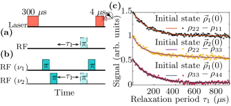
Figure 6: Pulse sequences used to prepare specific initial states and measure the population differences (a) $\text{$\rho{}_{22}$}(\tau_{1})-\text{$\rho{}_{11}$}(\tau_{1})$ and $\text{$\rho{}_{33}$}(\tau_{1})-\text{$\rho{}_{44}$}(\tau_{1})$, and (b) $\text{$\rho{}_{22}$}(\tau_{1})-\text{$\rho{}_{33}$}(\tau_{1})$. the laser and RF pulses are represented by the red and light green boxes. (c) Resulting experimental and calculated signals (from Eq. 12) of the population differences with the delay $\tau_{1}$.

High-quality measurements of the time dependence of individual populations are difficult. We therefore measure differences $\rho_{ii}-\rho_{kk}$ between populations. We start with two particularly simple time-dependences, which can be measured with the experiments shown in Fig. 6 (a) and (b). We first prepare an initial state with the populations $\vec{\rho_{1}}(0)=(0,0.5,0.5,0)^{\top}$, so that $c_{1}=-c_{2}=1$ and $c_{3}=c_{4}=0$, and the expected time-dependence is

$$\vec{\rho}(t)=\frac{1}{4}(\vec{u}_{1}-e^{\lambda_{2}t}\vec{u}_{2})=\frac{1}{4}\left(\begin{array}[]{c}1-e^{-\gamma t}\\ 1+e^{-\gamma t}\\ 1+e^{-\gamma t}\\ 1-e^{-\gamma t}\end{array}\right).$$ (13)

The pulse sequence for the preparation of the initial state $\vec{\rho_{{}_{1}}}(0)$ from the unpolarized state is shown in the first row of table 2: it consists of a laser pulse of duration 300 $\mu$s, which is long enough to drive the system to a steady state. After the state preparation, the system is allowed to relax for a time $\tau_{1}$. To read out the final state, we apply an RF pulse with flip-angle $\pi$ and record the PL during the measuring laser pulse. We subtract the result of this experiment from a similar experiment where the RF pulse was omitted. The resulting signal is proportional to the difference between the populations that were exchanged by the $\pi$ pulse. If the $\pi$-pulse is applied at frequency $\nu_{1}$, the signal is proportional to $\text{$\rho{}_{22}$}(\tau_{1})-\text{$\rho{}_{11}$}(\tau_{1})$ and if it is applied at $\nu_{3}$, the signal is proportional to $\text{$\rho{}_{33}$}(\tau_{1})-\text{$\rho{}_{44}$}(\tau_{1})$.

Figure 6 (c) shows the resulting signals for $\text{$\rho{}_{22}$}(\tau_{1})-\text{$\rho{}_{11}$}(\tau_{1})$ and $\text{$\rho{}_{33}$}(\tau_{1})-\text{$\rho{}_{44}$}(\tau_{1})$ as a function of the delay $\tau_{1}$. We fit the theoretical signal of Eq. (13) to the experimental signal. From the fits, we obtain the relaxation rate $\gamma=6.8\pm 0.2$ ms^-1, which corresponds to time constants $T_{1}^{12}$ = $T_{1}^{34}$=$1/\gamma$ =$146.2\pm 3.6$ $\mu$s at room temperature.

To determine the second rate constant $\alpha$, a different initial condition is needed. We chose $\vec{\rho_{2}}(0)=(0.5,0.5,0,0)^{\top}$ and measured the population difference $\rho_{22}-\rho_{33}$, which we expect to depend on the relaxation delay $\tau_{1}$ as

$$\rho_{22}(\tau_{1})-\rho_{33}(\tau_{1}) = \frac{\lambda_{3}(\alpha-\xi)e^{\lambda_{4}\tau_{1}}-\lambda_{4}(\alpha+\xi)e^{\lambda_{3}\tau_{1}}}{2\gamma\xi}.$$ (14)

The pulse sequence used to prepare the initial state $\vec{\rho_{2}}(0)$ from the thermal state is given in row 2 of Table 2 and in Figure 6 (b) which also shows the sequence for measuring the population difference $\rho_{22}-\rho_{33}$. For the initial state preparation, the 300 $\mu$s laser pulse, and two RF $\pi$ pulses were applied, one with frequency $\nu_{1}$ and a second with frequency $\nu_{2}$. Then the system was allowed to evolve for a time $\tau_{1}$ and another RF $\pi$-pulse with frequency $\nu_{1}$ and the signal measured using laser pulse. This experiment result was subtracted from a reference experiment with an additional $\pi$ pulse of frequency $\nu_{2}$ after the delay $\tau_{1}$, as indicated in Fig. 6 (b) by the dashed rectangle. Fig. 6 (c) depict the obtained signals for $\text{$\rho{}_{22}$}(\tau_{1})-\text{$\rho{}_{33}$}(\tau_{1})$ with the delay $\tau_{1}$. The theoretical signal of Eq. (14) was fitted to the experimental signals, using the value of $\gamma$ determined before. From the fits, we obtained the relaxation rate $\alpha=9.3\pm 0.4$ ms^-1 and the relaxation time $T_{1}^{23}$ = $1/\alpha$ =$107.3\pm 4.9$ $\mu$s at room temperature. The ratio $\alpha/\gamma=1.4\text{$\pm$}0.1$ agrees, within the experimental uncertainties, with the theoretical value of 4/3 (the ratio of the squares of the corresponding transition dipole moments) expected for relaxation by random magnetic fields coupling to the electron spin dipole moment Bloembergen et al. (1948).

V Optical spin alignment

V.1 Experiments

Initialization of quantum registers to a specific state is one of the primary requirements for the realization of any quantum device DiVincenzo (2000); Stolze and Suter (2008). The V${}_{Si}^{-}$ spin ensemble can be initialized into the $\pm$1/2 spin states of the electronic ground-state by laser illumination Baranov et al. (2011); Kraus et al. (2014); Singh et al. (2020). To determine the dynamics of this initialization process, we prepared the spin ensemble in different initial states, applied a laser pulse and again measured the populations $\vec{\rho}(t)$ as a function of the duration of the laser pulse. Figure 7 shows the pulse sequence used for preparing and measuring the population differences $\rho_{ii}-\rho_{jj}$ during optical pumping. First, we started with the unpolarized state $\vec{\rho}_{0}(0)=(1/4)(1,1,1,1)^{\top}$. The laser pulse of duration $t$ was applied, followed by the RF sequence given in Table 3 and the PL signal was measured during the readout pulse. This PL signal was subtracted from a reference PL signal measured by a similar experiment where no RF pulse was applied. The difference signal is proportional to $\rho_{ii}-\rho_{jj}$. For measuring the population differences $\rho_{22}-\rho_{11}$ and $\rho_{33}-\rho_{44}$, the same RF pulse sequences were used as in Sec. IV.2. For measuring the population difference $\rho_{22}-\rho_{44}$, the RF pulse sequence given in the third row of Table 3 was used i.e., a $\pi$ pulse with frequency $\nu_{2}$ followed by a $\pi$ pulse at frequency $\nu_{3}$. For measuring the population difference $\rho_{33}-\rho_{11}$, the RF pulse sequence is given in the fourth row of Table 3: A $\pi$ pulse at frequency $\nu_{2}$ is followed by another $\pi$ pulse at frequency $\nu_{1}$. The experimental data $(S_{\rho_{ii}-\rho_{jj}}(t))$ were scaled by multiplying them with a constant factor $N$ such that the signal for $\rho_{33}-\rho_{44}$ of the stationary state (22) prepared by a 300 $\mu$s laser pulse matches the theoretically expected value of 0.37:

$$\rho_{ii}-\rho_{jj}(t)=NS_{\rho_{ii}-\rho_{jj}}(t).$$ (15)

While the absolute scale of the signal is not important for the goal of determining the rate constants, we use this scaling which fixes the absolute values of the populations and allows a unique comparison between the theoretical model and the experimental data. The resulting normalized signals $\rho_{ii}-\rho_{jj}$ are shown in Fig. 8(a).

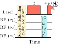
Figure 7: Pulse sequence scheme used to prepare specific initial states and measure the evolution of the population difference $\rho_{ii}-\rho_{jj}$ during optical pumping. Details of the initialization sequence are given in Table II and for the readout sequence in table III.

S. No	Population difference	Pulse sequence
1	$\rho_{22}-\rho_{11}$	$R^{\nu_{1}}$
2	$\rho_{33}-\rho_{44}$	$R^{\nu_{3}}$
3	$\rho_{22}-\rho_{44}$	$R^{\nu_{2}}R^{\nu_{3}}$
4	$\rho_{33}-\rho_{11}$	$R^{\nu_{2}}$$R^{\nu_{1}}$

Table 3: Readout pulse sequences used to measure different population differences. $R^{\nu_{i}}$ are RF pulses with frequency $\nu_{i}$ and flip angle $\pi$.

When the V${}_{Si}^{-}$ is excited with a non resonant laser, the shelving states also populate the $m_{s}=\pm 3/2$ states, and the resulting spin polarization ($P$) is reduced Nagy et al. (2019). In this more general case, the population vector can be written as

$$\vec{\sigma}=\frac{1-P}{4}\hat{I}+P\vec{\rho},$$ (16)

and the polarization $P$ has been estimated as $\approx$80% Soltamov et al. (2012). Here, $\vec{\sigma}$ represents the total ensemble’s population vector, and $\vec{\rho}=(\rho_{11},\rho_{22},\rho_{33},\rho_{44})^{\top}$ is the population vector of the spin-polarized sub-ensemble, which can be manipulated by RF pulses. All four populations $\rho_{11}$, $\rho_{22}$, $\rho_{33}$ and $\rho_{44}$ could be determined individually from the four experiments described above and using the normalization condition $\rho_{11}+\rho_{22}+\rho_{33}+\rho_{44}=1$.

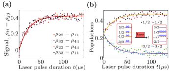
Figure 8: (a) Population differences $\rho_{ii}-\rho_{jj}$, vs. laser pulse duration $t$. Stars, squares, diamonds and circles represent the experimentally measured signal for the population differences. The red curve represents the analytical solution, obtained by solving Eq. 23 when the system is initially unpolarized. (b) Populations as a function of the laser pulse duration $t$, starting from the unpolarized state.

Figure 8(b) shows the evolution of the populations of the spin states during the laser pulse. Starting from the unpolarized state where all populations are $\rho_{ii}=1/4$, the populations $\rho_{22}$ and $\rho_{33}$ grow to a limiting value of $\approx 0.44$ while the populations $\rho_{11}$ and $\rho_{44}$ decrease to a limiting value of $\approx 0.06.$

Figure 9: a), b) : Population differences $\rho_{22}-\rho_{11}$, $\rho_{33}-\rho_{44}$, $\rho_{22}-\rho_{44}$, and $\rho_{33}-\rho_{11}$ as a function of the laser pulse duration $t$. The experimental data are represented as points and the corresponding analytical solutions Eq. (23) as curves. In (a), the initial condition was $\vec{\rho}_{3exp}(0)=(0.03,0.47,0.11,0.39)^{\top}$ and in (b) $\vec{\rho}_{4exp}(0)=(0.06,0.16,0.36,0.42)^{\top}$. c), d) : Populations as a function of the laser pulse duration $t$, for the initial state (c) $\vec{\rho}_{3exp}$ and (d) $\vec{\rho}_{4exp}$.

We repeated the experiment of Fig. 7, with different initial conditions: $\vec{\rho}_{3}(0)=(0,0.5,0,0.5)^{\top}$ and $\vec{\rho_{4}}(0)=(0,0,0.5,0.5)^{\top}$. The pulse sequences used for the preparation of these initial states are given in the third and forth row of Table 2, respectively. The corresponding results are shown in figures 9(a) and (b). From the measured population differences, we reconstructed the time-dependence of the populations, which are shown in Fig. 9(c) and (d), as a function of the laser pulse duration $t$. The experimentally prepared initial states were $\vec{\rho}_{3exp}(0)=(0.03,0.47,0.11,0.39)^{\top}$ and $\vec{\rho}_{4exp}(0)=(0.06,0.16,0.36,0.42)^{\top}$. One of the main reasons for the deviations of the experimentally prepared states from the theoretical states is the limited laser intensity, which results in incomplete polarisation. This could be improved by using a tighter focus of the laser beam. Other causes are imperfections in the RF pulses and relaxation.

V.2 Model and rate constants

The laser pulse transfers population from the spin-levels $|\pm\frac{3}{2}\rangle$ through the shelving state to $|\pm\frac{1}{2}\rangle$, as indicated in Fig. 8 (b). Figures 8 and 9 show that during the laser pulse, the populations of the $|\pm\frac{1}{2}\rangle$ states increase to values close to 0.5, while the populations of the $|\pm\frac{3}{2}\rangle$ states are strongly depleted.

Based on these experimental results and assuming that the lifetimes in the excited state and the shelving states are short compared to the pumping time, we use the following equations for modeling the dynamics of the system:

$$\frac{d}{dt}\vec{\rho} =$$

$$\frac{1}{2}\left(\begin{array}[]{cccc}-\gamma-2\delta&\gamma\\ \gamma+\delta&-\alpha-\gamma-\delta&\alpha+\delta&\delta\\ \delta&\alpha+\delta&-\alpha-\gamma-\delta&\gamma+\delta\\ &&\gamma&-\gamma-2\delta\end{array}\right)\vec{\rho}$$ (21)

where $\delta$ is the rate at which population is pumped from the states $|\pm 3/2\rangle$ to $|\pm 1/2\rangle$. The resulting stationary state is

$$\vec{\rho}_{st}=\frac{\gamma}{4(\gamma+\delta)}\left(\begin{array}[]{c}1\\ 1\\ 1\\ 1\end{array}\right)+\frac{\delta}{2(\gamma+\delta)}\left(\begin{array}[]{c}0\\ 1\\ 1\\ 0\end{array}\right),$$ (22)

which approaches $(0,\frac{1}{2},\frac{1}{2},0)^{\top}$ for $\delta\gg\gamma$.

The eigenvalues and eigenvectors for Eq. (21) are

$$\vec{\lambda}^{op}=\left(\begin{array}[]{c}0\\ -\gamma-\delta\\ -\frac{\alpha+\gamma+\xi}{2}-\delta\\ -\frac{\alpha+\gamma-\xi}{2}-\delta\end{array}\right)$$

$\begin{aligned} \vec{v}_{i}=&\left\{\begin{aligned} \left(\begin{array}[]{c}1\\ \frac{\gamma+2\delta}{\gamma}\\ \frac{\gamma+2\delta}{\gamma}\\ 1\end{array}\right),\left(\begin{array}[]{c}1\\ -1\\ -1\\ 1\end{array}\right),&\left(\begin{array}[]{c}-1\\ \frac{\alpha^{2}+\xi(\delta+\alpha)+\delta(\alpha-\gamma)}{\alpha\gamma+\delta(\alpha+\gamma-\xi)}\\ -\frac{\alpha+\xi}{\gamma}\\ 1\end{array}\right),\\ \left(\begin{array}[]{c}-1\\ \frac{\alpha^{2}-\xi(\delta+\alpha)+\delta(\alpha-\gamma)}{\alpha\gamma+\delta(\alpha+\gamma+\xi)}\\ \frac{-\alpha+\xi}{\gamma}\\ 1\end{array}\right)\end{aligned}\right\}\end{aligned},$ respectively. The solution of Eq. (21) for an initial state $\vec{\rho}(0)=(a,b,c,d)^{\top}$ is

$$\vec{\rho}(t)=\frac{1}{4}\sum p_{i}e^{\lambda_{i}^{op}t}\vec{v}_{i}$$ (23)

where

$$p_{1} = \frac{\gamma}{\gamma+\delta},$$

$$p_{2} = \frac{\gamma(a-b-c+d)+2\delta(a+d)}{\gamma+\delta},$$

$$p_{3} = \frac{\gamma(b-c)-(\xi-\alpha)(a-d)}{\xi},$$

$$p_{4} = \frac{\gamma(c-b)-(\xi+\alpha)(a-d)}{\xi}.$$

The resulting expressions for the case where the initial state is the depolarised state is given in Appendix D. The calculated population differences are plotted in Figures 8 (a), 9 (a) and (b), and the populations in Figures 8 (b), 9 (c) and (d). The best fits with the experimental data, which were measured with a laser intensity $I=$ 622.64 W/cm² were obtained for the rate constant $\delta$ = $39\pm 3$ $m$s^-1. For $\alpha$ and $\gamma$, we used the values determined in section IV.

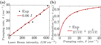
Figure 10: Plot of (a) pumping rates with the laser beam intensity, (b) polarization with pumping rate.

Taking additional data with different laser intensities, we found that the pumping rate $\delta$ increases linearly with the intensity, i.e., $\delta(\mathrm{ms^{-1}})=0.06\pm 0.01$ $I$ (W cm^-2), as shown in Fig. 10 (a). This indicates that at the rate is limited by the population of the shelving state, which is far from being saturated under our experimental conditions. Figure 10 (b) shows the spin polarization, measured as the sum of the $\pm$1/2 states after a laser pulse of 300 $\mu$s as a function of the pumping rate $\delta$.

VI Discussion and Conclusion

Silicon vacancy centers in SiC have shown promising results for quantum sensing, single-photon emitters, and applications as light-matter interfaces and other quantum technologies. In this work, we have demonstrated the coherent control of all four levels of the V₁/ V₃ type V${}_{Si}^{-}$. We measured the Rabi frequency of all three RF transitions and the corresponding relaxation rates $\alpha$ (for $|+1/2>$ $\leftrightarrow$ $|-1/2\rangle$ ) and $\gamma$ (for $|\pm 3/2>$ $\leftrightarrow$ $|\pm 1/2\rangle$ ) by fitting the data with the proposed relaxation model. In general, the relaxation of a spin 3/2 system can be described by three relaxation modes with three time constants, which have been termed the spin dipole ($T_{p}$), quadrupole ($T_{d}$) and octupole ($T_{f}$) Soltamov et al. (2019); Tarasenko et al. (2018); Ramsay and Rossi (2020); van der Maarel (2003). For a dipole like perturbation the spin-relaxation times are $T_{p}$/3=$T_{d}$=2$T_{f}$, $\alpha=(2/3)T_{d}^{-1}$ and $\gamma=(1/2)T_{d}^{-1}$ as discussed theoretically in the case of a fluctuating magnetic field acting on a V${}_{Si}^{-}$ in SiC Bloembergen et al. (1948); Soltamov et al. (2019). The ratio of the experimentally measured values of $\alpha$ and $\gamma$ is close to this theoretical value. It has recently been demonstrated that for $V_{2}$ type V${}_{Si}^{-}$ in 4H-SiC, this is not the case due to mixing the octupole and dipole relaxation modes since a perturbation with dipole symmetry cannot mix different order poles Ramsay and Rossi (2020).

We also determined the dynamics of the optical initialization process by preparing the system in three different initial states and measuring the population dynamics during a laser pulse. The laser illumination transfers the population from $\pm$3/2 to $\pm$1/2 spin states for all three initial states. To interpret the resulting data, we proposed a simple rate equation model for this process and were able to determine all relevant rate constants from the experimental data. According to Fig. 10 (b), the spin polarisation of subensemble $\rho$ approaches unity at intensitites > 200 W/cm². As mentioned above, with the non-resonant laser excitation, the shelving states also populate the ± 3/2 states, resulting in reduced spin polarization of the total ensemble $\sigma$, which can be improved by using resonant optical excitation Nagy et al. (2019). In conclusion, we are confident that our results will contribute to a better understanding of this fascinating system and open the way to more useful applications.

Appendix A: sample preparation

The experiments were carried out on the same sample as used in our previous work  Singh et al. (2020). This sample is isotopically enriched in ²⁸Si and ¹³C. As the source of a ²⁸Si isotope, pre-prepared silicon available in the form of small pieces (1-3 mm) with an isotope composition of 99.999% ²⁸Si was used. Carbon powder enriched to 15% in ¹³C was used as the ¹³C source. The SiC crystal was grown in a laboratory. The SiC crystal was grown at a growth rate of $\approx$ 100$\mu$m/h on a (0001) Si face at a temperature of 2300°-2400°C in an argon atmosphere. Following the growth of the SiC crystal, the wafer was machined and cut. At room temperature, the crystal was irradiated with electrons of an energy 2 MeV and with a dose of 10¹⁸cm^-2 to create V${}_{Si}^{-}$ centers.

Appendix B: ODMR setup

Figure 11: Experimental setup for measuring ODMR. The laser beam is represented by the red line from the laser. The laser pulses are produced by the acousto-optical modulator (AOM). A long-pass filter, convex lenses, and a mirrors are defined by the ellipsoids named F, L, and M, respectively. The RF is applied using a three-turn Helmholtz coil-pair made of 100 $\mu$m diameter copper wire placed perpendicular to the $c$-axis, in series with a 50 $\Omega$ resistor which is labeled R. The SiC sample is the gray rectangle labeled S that is positioned between the RF coils. Helmholtz coils for producing a static magnetic field in any direction are represented by the three orthogonal ring-pairs Cx, Cy, and Cz. A digital word generator, an avalanche photodetector module, and direct digital synthesizers are represented by rounded rectangles labeled DWG, APD, and DDS, respectively.

Figure 11 shows the setup used for the cw- and time-resolved ODMR measurements. A 785 nm laser diode (LD785-SE400) was used for the optical excitation source. An acousto-optical modulator (AOM; NEC model OD8813A) used for producing laser pulses. An RF switch (Mini-Circuits ZASWA-2-50DR+, dc-5 GHz) was used to produce the RF pulses. The Transistor-transistor logic pulses that control the timing were produced by a digital word generator (DWG; SpinCore PulseBlaster ESR-PRO PCI card). For applying the static magnetic field in any direction, we used three orthogonal Helmholtz coil-pairs. Currents up to 15A are delivered to the coils by current source (Servowatt, three-channel DCP-390/30). An analog control voltage was used to control the currents individually. Analog Devices AD9915 direct digital synthesizer (DDS) provided the RF signal, which can generate signals up to 1 GHz. The RF pulses were created by an RF switch, amplified by a Mini-Circuits LZY-1 50 W amplifier, and applied to the SiC sample through a handmade Helmholtz-pair of RF coils with a diameter of 2.5 mm and three turns in each coil made from 100 $\mu$m diameter wire terminated with a 50 $\Omega$ resistor. A convex lens (L3 in Fig. 11) with a focal length of 20 cm was used to focused a laser light on the sample. Two lenses L1 and L2, respectively, used to collect the PL. An avalanche photodiode (APD) module (C12703 series from Hamamatsu) used to record PL signal which was pass before through an 850 nm long-pass filter. A USB card (PicoScope 2000 series) connected to a device (for pulsed measurements) or a lock-in amplifier (SRS model SR830 DSP) for cw-ODMR was used to record the signal from the APD. To measure the cw-ODMR signal, we used the setup shown in Fig. 11, with the RF switched on for continuous laser irradiation and the APD connected to the lock-in amplifier. The DWG modulate the amplitude of the RF and the APD signal was demodulated with the lock-in amplifier whose reference signal was supplied by the DWG.

For the time-resolved ODMR, the APD shown in Fig. 11 was connected to the Picoscope USB card. The RF pulses were generated using DDSes and RF switches and applied between the state initialization and measurement.

Appendix C: POWER DEPENDENCE OF RABI OSCILLATIONS

Rabi with RF Power

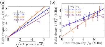
Figure 12: (a) Plot of the experimentally measured Rabi frequency vs the square root of RF Power. (b) Plot of the Rabi decay time $T_{2}^{R}$ of different transitions vs the Rabi frequency.

Transitions	$r_{i}$	$m_{i}$	$c_{i}$
$\nu_{1}$	$1.168\pm 0.062$	$0.35\pm 0.13$	$1.45\pm 0.66$
$\nu_{2}$	$1.352\pm 0.106$	$0.53\pm 0.24$	$0.07\pm 1.24$
$\nu_{3}$	$1.006\pm 0.041$	$0.22\pm 0.16$	$1.62\pm 0.84$

Table 4: Fitting parameters of Eqns 24 and 25 for the different transitions of the V₁/ V₃ type V${}_{Si}^{-}$.

Figure 12(a) shows the measured Rabi frequencies of the $\nu_{1}$, $\nu_{2}$ and $\nu_{3}$ transitions measured versus the square root of the applied RF power. For fitting the experimental data we used the following function

$$f_{R}(\sqrt{RF\>power})=r_{i}\sqrt{RF\>power}.$$ (24)

The fit parameters $r_{i}$ are given in the second column of Table 4 for the $\nu_{1}$, $\nu_{2}$, and $\nu_{3}$ transitions. The ratio of the 3 Rabi frequencies is 1.173$\pm 0.164$ : 2 : 1.149$\pm 0.132$, which is close to the theoretically expected value of $\sqrt{3}$ : $2$ : $\sqrt{3}$, i.e., the ratio of the transition dipole matrix elements of a spin 3/2 Ramsay and Rossi (2020); Mizuochi et al. (2002). The deviation appears to be related to reflections in the circuit that feeds RF power to the sample, which generates standing waves and increases with the RF frequency. In Fig. 12 (a), we measured the forward RF power instead of actual RF current in the coil, which is not easily accessible. Figure 12(b) shows the plot of the Rabi decay times of the $\nu_{1}$, $\nu_{2}$ and $\nu_{3}$ transitions at different Rabi frequencies. The experimental data were fitted to the function

$$\frac{1}{T_{2}^{R}}(f_{R})=m_{i}f_{R}+c_{i}$$ (25)

The fitted parameters $m_{i}$ and $c_{i}$ are given in the third and fourth columns of Table 4 for the $\nu_{1}$, $\nu_{2}$, and $\nu_{3}$ transitions. The differences between the $T_{2}^{R}$ of $\nu_{1}$ and $\nu_{3}$ transitions are within the error margins and appear not significant. At the lower Rabi frequency, the longer dephasing time $T_{2}^{R}$ for the transition $\nu_{2}$ is expected as it is less affected by inhomogeneous broadening than the two transitions $\nu_{1}$ and $\nu_{3}$ Eickhoff and Suter (2004); Soltamov et al. (2019).

Appendix D: Time dependences for specific initial conditions

This section provides two specific solutions for the population dynamics without and with the laser field, for 2 different initial conditions. For the initial state $\vec{\rho_{2}}(0)=\text{$\frac{1}{2}$}(1,1,0,0)^{\top}$, the solution of the relaxation dynamics Eq. (12) is

$$\rho_{11}(t) = \frac{\lambda_{3}e^{\lambda_{4}t}+\lambda_{4}e^{\lambda_{3}t}+\xi}{4\xi};$$

$$\rho_{22}(t) = \frac{\lambda_{3}(\alpha-\xi)e^{\lambda_{4}t}-\lambda_{4}(\alpha+\xi)e^{\lambda_{3}t}+\gamma\xi}{4\gamma\xi};$$

$$\rho_{33}(t) = \frac{\lambda_{3}(-\alpha+\xi)e^{\lambda_{4}t}+\lambda_{4}(\alpha+\xi)e^{\lambda_{3}t}+\gamma\xi}{4\gamma\xi};$$

$$\rho_{44}(t) = \frac{-\lambda_{3}e^{\lambda_{4}t}+\lambda_{4}e^{\lambda_{3}t}+\xi}{4\xi}.$$

For the initial state $\vec{\rho_{0}}(0)=\frac{1}{4}(1,1,1,1)^{\top}$, the solution of of the optical pumping dynamics Eq. (23) is

$$\rho_{11} = \rho_{44}=-\frac{\gamma+\delta e^{\lambda_{2}^{op}t}}{4\lambda_{2}^{op}},$$ (26)

$$\rho_{22} = \rho_{33}=-\frac{\gamma+2\delta-\delta e^{\lambda_{2}^{op}t}}{4\lambda_{2}^{op}}.$$ (27)

References

- Falk et al. (2013) A. L. Falk, B. B. Buckley, G. Calusine, W. F. Koehl, V. V. Dobrovitski, A. Politi, C. A. Zorman, P. X.-L. Feng, and D. D. Awschalom, Nature communications 4, 1819 (2013).
- Widmann et al. (2015) M. Widmann, S.-Y. Lee, T. Rendler, N. T. Son, H. Fedder, S. Paik, L.-P. Yang, N. Zhao, S. Yang, I. Booker, et al., Nature materials 14, 164 (2015).
- Christle et al. (2015) D. J. Christle, A. L. Falk, P. Andrich, P. V. Klimov, J. U. Hassan, N. T. Son, E. Janzén, T. Ohshima, and D. D. Awschalom, Nature materials 14, 160 (2015).
- Baranov et al. (2013) P. Baranov, V. A. Soltamov, A. A. Soltamova, G. V. Astakhov, and V. D. Dyakonov, in Silicon Carbide and Related Materials 2012, Materials Science Forum, Vol. 740 (Trans Tech Publications Ltd, 2013) pp. 425–430.
- Anisimov et al. (2018) A. N. Anisimov, V. A. Soltamov, I. D. Breev, R. A. Babunts, E. N. Mokhov, G. V. Astakhov, V. Dyakonov, D. R. Yakovlev, D. Suter, and P. G. Baranov, AIP Advances 8, 085304 (2018).
- Anisimov et al. (2016) A. Anisimov, D. Simin, V. A. Soltamov, S. P. Lebedev, P. G. Baranov, G. V. Astakhov, and V. Dyakonov, Scientific reports 6, 33301 (2016).
- Koehl et al. (2011) W. F. Koehl, B. B. Buckley, F. J. Heremans, G. Calusine, and D. D. Awschalom, Nature 479, 84 (2011).
- Riedel et al. (2012) D. Riedel, F. Fuchs, H. Kraus, S. Väth, A. Sperlich, V. Dyakonov, A. A. Soltamova, P. G. Baranov, V. A. Ilyin, and G. V. Astakhov, Physical review letters 109, 226402 (2012).
- Soykal et al. (2016) O. O. Soykal, P. Dev, and S. E. Economou, Physical Review B 93, 081207(R) (2016).
- Doherty et al. (2013) M. W. Doherty, N. B. Manson, P. Delaney, F. Jelezko, J. Wrachtrup, and L. C. Hollenberg, Physics Reports 528, 1 (2013).
- Suter and Jelezko (2017) D. Suter and F. Jelezko, Progress in nuclear magnetic resonance spectroscopy 98, 50 (2017).
- Suter (2020) D. Suter, Magnetic Resonance 1, 115 (2020).
- Falk et al. (2015) A. L. Falk, P. V. Klimov, V. Ivády, K. Szász, D. J. Christle, W. F. Koehl, A. Gali, and D. D. Awschalom, Phys. Rev. Lett. 114, 247603 (2015).
- Yan et al. (2018) F.-F. Yan, J.-F. Wang, Q. Li, Z.-D. Cheng, J.-M. Cui, W.-Z. Liu, J.-S. Xu, C.-F. Li, and G.-C. Guo, Phys. Rev. Applied 10, 044042 (2018).
- Falk et al. (2014) A. L. Falk, P. V. Klimov, B. B. Buckley, V. Ivády, I. A. Abrikosov, G. Calusine, W. F. Koehl, A. Gali, and D. D. Awschalom, Phys. Rev. Lett. 112, 187601 (2014).
- Soltamov et al. (2012) V. A. Soltamov, A. A. Soltamova, P. G. Baranov, and I. I. Proskuryakov, Phys. Rev. Lett. 108, 226402 (2012).
- Biktagirov et al. (2018) T. Biktagirov, W. G. Schmidt, U. Gerstmann, B. Yavkin, S. Orlinskii, P. Baranov, V. Dyakonov, and V. Soltamov, Phys. Rev. B 98, 195204 (2018).
- Sörman et al. (2000) E. Sörman, N. T. Son, W. M. Chen, O. Kordina, C. Hallin, and E. Janzén, Phys. Rev. B 61, 2613 (2000).
- Davidsson et al. (2019) J. Davidsson, V. Ivády, R. Armiento, T. Ohshima, N. T. Son, A. Gali, and I. A. Abrikosov, Applied Physics Letters 114, 112107 (2019), https://doi.org/10.1063/1.5083031 .
- Singh et al. (2020) H. Singh, A. N. Anisimov, S. S. Nagalyuk, E. N. Mokhov, P. G. Baranov, and D. Suter, Phys. Rev. B 101, 134110 (2020).
- Nagy et al. (2019) R. Nagy, M. Niethammer, M. Widmann, Y.-C. Chen, P. Udvarhelyi, C. Bonato, J. U. Hassan, R. Karhu, I. G. Ivanov, N. T. Son, et al., Nature communications 10, 1954 (2019).
- Simin et al. (2017) D. Simin, H. Kraus, A. Sperlich, T. Ohshima, G. V. Astakhov, and V. Dyakonov, Phys. Rev. B 95, 161201(R) (2017).
- Kraus et al. (2014) H. Kraus, V. Soltamov, D. Riedel, S. Väth, F. Fuchs, A. Sperlich, P. Baranov, V. Dyakonov, and G. Astakhov, Nature Physics 10, 157 (2014).
- Bathen et al. (2019) M. E. Bathen, A. Galeckas, J. Müting, H. M. Ayedh, U. Grossner, J. Coutinho, Y. K. Frodason, and L. Vines, npj Quantum Information 5, 1 (2019).
- Soltamov et al. (2019) V. Soltamov, C. Kasper, A. Poshakinskiy, A. Anisimov, E. Mokhov, A. Sperlich, S. Tarasenko, P. Baranov, G. Astakhov, and V. Dyakonov, Nature communications 10, 1678 (2019).
- Yang et al. (2014) L.-P. Yang, C. Burk, M. Widmann, S.-Y. Lee, J. Wrachtrup, and N. Zhao, Phys. Rev. B 90, 241203(R) (2014).
- Baranov et al. (2011) P. G. Baranov, A. P. Bundakova, A. A. Soltamova, S. B. Orlinskii, I. V. Borovykh, R. Zondervan, R. Verberk, and J. Schmidt, Phys. Rev. B 83, 125203 (2011).
- Fuchs et al. (2015) F. Fuchs, B. Stender, M. Trupke, D. Simin, J. Pflaum, V. Dyakonov, and G. Astakhov, Nature communications 6, 7578 (2015).
- Astakhov et al. (2016) G. Astakhov, D. Simin, V. Dyakonov, B. Yavkin, S. Orlinskii, I. Proskuryakov, A. Anisimov, V. Soltamov, and P. Baranov, Applied Magnetic Resonance 47, 793 (2016).
- Hain et al. (2014) T. C. Hain, F. Fuchs, V. A. Soltamov, P. G. Baranov, G. V. Astakhov, T. Hertel, and V. Dyakonov, Journal of Applied Physics 115, 133508 (2014).
- Chen (2003) W. M. Chen, “Optically detected magnetic resonance of defects in semiconductors,” in EPR of Free Radicals in Solids: Trends in Methods and Applications, edited by A. Lund and M. Shiotani (Springer US, Boston, MA, 2003) pp. 601–625.
- Depinna and Cavenett (1982) S. Depinna and B. Cavenett, Journal of Physics C: Solid State Physics 15, L489 (1982).
- Langof et al. (2002) L. Langof, E. Ehrenfreund, E. Lifshitz, O. I. Micic, and A. J. Nozik, The Journal of Physical Chemistry B 106, 1606 (2002).
- Carter et al. (2015) S. G. Carter, O. O. Soykal, P. Dev, S. E. Economou, and E. R. Glaser, Phys. Rev. B 92, 161202(R) (2015).
- Ramsey (1950) N. F. Ramsey, Phys. Rev. 78, 695 (1950).
- Eickhoff and Suter (2004) M. Eickhoff and D. Suter, Journal of Magnetic Resonance 166, 69 (2004).
- Hahn (1950) E. L. Hahn, Phys. Rev. 80, 580 (1950).
- Bloembergen et al. (1948) N. Bloembergen, E. M. Purcell, and R. V. Pound, Phys. Rev. 73, 679 (1948).
- Abragam (1961) A. Abragam, The principles of nuclear magnetism (Oxford University Press, UK, 1961).
- DiVincenzo (2000) D. P. DiVincenzo, Fortschritte der Physik: Progress of Physics 48, 771 (2000).
- Stolze and Suter (2008) J. Stolze and D. Suter, Quantum Computing: A Short Course from Theory to Experiment, 2nd ed. (Wiley-VCH, Berlin, 2008).
- Tarasenko et al. (2018) S. A. Tarasenko, A. V. Poshakinskiy, D. Simin, V. A. Soltamov, E. N. Mokhov, P. G. Baranov, V. Dyakonov, and G. V. Astakhov, physica status solidi (b) 255, 1870101 (2018), https://onlinelibrary.wiley.com/doi/pdf/10.1002/pssb.201870101 .
- Ramsay and Rossi (2020) A. J. Ramsay and A. Rossi, Phys. Rev. B 101, 165307 (2020).
- van der Maarel (2003) J. R. van der Maarel, Concepts in Magnetic Resonance Part A 19A, 97 (2003), https://onlinelibrary.wiley.com/doi/pdf/10.1002/cmr.a.10087 .
- Mizuochi et al. (2002) N. Mizuochi, S. Yamasaki, H. Takizawa, N. Morishita, T. Ohshima, H. Itoh, and J. Isoya, Phys. Rev. B 66, 235202 (2002).