Kronecker Attention Networks

Abstract.

Attention operators have been applied on both 1-D data like texts and higher-order data such as images and videos. Use of attention operators on high-order data requires flattening of the spatial or spatial-temporal dimensions into a vector, which is assumed to follow a multivariate normal distribution. This not only incurs excessive requirements on computational resources, but also fails to preserve structures in data. In this work, we propose to avoid flattening by assuming the data follow matrix-variate normal distributions. Based on this new view, we develop Kronecker attention operators (KAOs) that operate on high-order tensor data directly. More importantly, the proposed KAOs lead to dramatic reductions in computational resources. Experimental results show that our methods reduce the amount of required computational resources by a factor of hundreds, with larger factors for higher-dimensional and higher-order data. Results also show that networks with KAOs outperform models without attention, while achieving competitive performance as those with original attention operators.

1. Introduction

Deep neural networks with attention operators have shown great capability of solving challenging tasks in various fields, such as natural language processing (Bahdanau et al., 2015; Vaswani et al., 2017; Johnson and Zhang, 2015), computer vision (Xu et al., 2015; Lu et al., 2016), and network embedding (Veličković et al., 2017; Gao et al., 2018b). Attention operators are able to capture long-range dependencies, resulting in significant performance boost (Li et al., 2018; Malinowski et al., 2018). While attention operators were originally proposed for 1-D data, recent studies (Wang et al., 2018; Zhao et al., 2018; Gao and Ji, 2019) have attempted to apply them on high-order data, such as images and videos. However, a practical challenge of using attention operators on high-order data is the excessive requirement computational resources, including computational cost and memory usage. For example, for 2-D image tasks, the time and space complexities are both quadratic to the product of the height and width of the input feature maps. This bottleneck becomes increasingly severe as the spatial or spatial-temporal dimensions and the order of input data increase. Prior methods address this problem by either down-sampling data before attention operators (Wang et al., 2018) or limiting the path of attention (Huang et al., 2018).

In this work, we propose novel and efficient attention operators, known as Kronecker attention operators (KAOs), for high-order data. We investigate the above problem from a probabilistic perspective. Specifically, regular attention operators flatten the data and assume the flattened data follow multivariate normal distributions. This assumption not only results in high computational cost and memory usage, but also fails to preserve the spatial or spatial-temporal structures of data. We instead propose to use matrix-variate normal distributions to model the data, where the Kronecker covariance structure is able to capture relationships among spatial or spatial-temporal dimensions. Based on this new view, we propose our KAOs, which avoid flattening and operate on high-order data directly. Experimental results show that KAOs are as effective as original attention operators, while dramatically reducing the amount of required computational resources. In particular, we employ KAOs to design a family of efficient modules, leading to our compact deep models known as Kronecker attention networks (KANets). KANets significantly outperform prior compact models on the image classification task, with fewer parameters and less computational cost. Additionally, we perform experiments on image segmentation tasks to demonstrate the effectiveness of our methods in general application scenarios.

2. Background and Related Work

[]

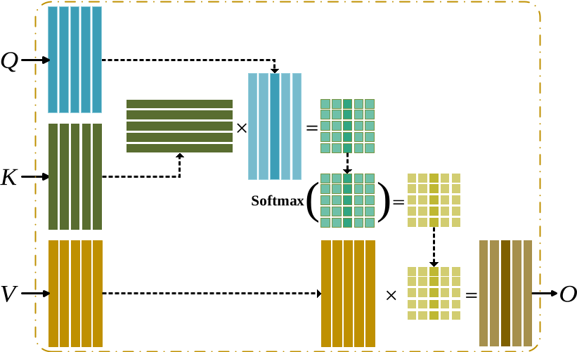
Figure 1. An illustration of the attention operator. Here, $\times$ denotes matrix multiplication, and softmax($\cdot$) is the column-wise softmax operator. $\boldsymbol{Q}$, $\boldsymbol{K}$, and $\boldsymbol{V}$ are input matrices. A similarity score is computed between each query vector as a column of $\boldsymbol{Q}$ and each key vector as a column in $\boldsymbol{K}$. Softmax($\cdot$) normalizes these scores and makes them sum to 1. Multiplication between normalized scores and the matrix $\boldsymbol{V}$ yields the corresponding output vector.

In this section, we describe the attention and related non-local operators, which have been applied on various types of data such as texts, images and videos.

2.1. Attention Operator

The inputs to an attention operator include a query matrix $\boldsymbol{Q}=[\mathbf{q}_{1},\mathbf{q}_{2},\cdots,\mathbf{q}_{m}]\in\mathbb{R}^{d\times m}$ with each $\mathbf{q}_{i}\in\mathbb{R}^{d}$, a key matrix $\boldsymbol{K}=[\mathbf{k}_{1},\mathbf{k}_{2},\cdots,\mathbf{k}_{n}]\in\mathbb{R}^{d\times n}$ with each $\mathbf{k}_{i}\in\mathbb{R}^{d}$, and a value matrix $\boldsymbol{V}=[\mathbf{v}_{1},\mathbf{v}_{2},\cdots,\mathbf{v}_{n}]\in\mathbb{R}^{p\times n}$ with each $\mathbf{v}_{i}\in\mathbb{R}^{p}$. The attention operation computes the responses of a query vector $\mathbf{q}_{i}$ by attending it to all key vectors in $\boldsymbol{K}$ and uses the results to take a weighted sum over value vectors in $\boldsymbol{V}$. The layer-wise forward-propagation operation of an attention operator can be expressed as

(1) $$\boldsymbol{O}=\mbox{attn}(\boldsymbol{Q},\boldsymbol{K},\boldsymbol{V})=\boldsymbol{V}\times\mbox{Softmax}(\boldsymbol{K}^{T}\boldsymbol{Q}).$$

Matrix multiplication between $\boldsymbol{K}^{T}$ and $\boldsymbol{Q}$ results in a coefficient matrix $\boldsymbol{E}=\boldsymbol{K}^{T}\boldsymbol{Q}$, in which each element $e_{ij}$ is calculated by the inner product between $\mathbf{k}_{i}^{T}$ and $\mathbf{q}_{j}$. This coefficient matrix $\boldsymbol{E}$ computes similarity scores between every query vector $\mathbf{q}_{i}$, and every key vector $\mathbf{k}_{j}$ and is normalized by a column-wise softmax operator to make every column sum to 1. The output $\boldsymbol{O}\in\mathbb{R}^{p\times m}$ is obtained by multiplying $\boldsymbol{V}$ with the normalized $\boldsymbol{E}$. In self-attention operators (Vaswani et al., 2017), we have $\boldsymbol{Q}=\boldsymbol{K}=\boldsymbol{V}$. Figure 1 provides an illustration of the attention operator. The computational cost in Eq. 1 is $O(m\times n\times(d+p))$. The memory required for storing the intermediate coefficient matrix $\boldsymbol{E}$ is $O(mn)$. If $d=p$ and $m=n$, the time and space complexities become $O(m^{2}\times d)$ and $O(m^{2})$, respectively.

There are several other ways to compute $\boldsymbol{E}$ from $\boldsymbol{Q}$ and $\boldsymbol{K}$, including Gaussian function, dot product, concatenation, and embedded Gaussian function. It has been shown that dot product is the simplest but most effective one (Wang et al., 2018). Therefore, we focus on the dot product similarity function in this work.

In practice, we can first perform separate linear transformations on each input matrix, resulting in the following attention operator: $\boldsymbol{O}=\boldsymbol{W}^{V}\boldsymbol{V}\mbox{Softmax}((\boldsymbol{W}^{K}\boldsymbol{K})^{T}\boldsymbol{W}^{Q}\boldsymbol{Q})$, where $\boldsymbol{W}^{V}\in\mathbb{R}^{p^{\prime}\times p}$, $\boldsymbol{W}^{K}\in\mathbb{R}^{d^{\prime}\times d}$, and $\boldsymbol{W}^{Q}\in\mathbb{R}^{d^{\prime}\times d}$. For notational simplicity, we omit linear transformations in the following discussion.

2.2. Non-Local Operator

[]

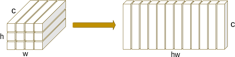
Figure 2. Conversion of a third-order tensor into a matrix by unfolding along mode-3. In this example, a $h\times w\times c$ tensor is unfolded into a $c\times hw$ matrix.

Non-local operators, which is proposed in (Wang et al., 2018), apply self-attention operators on higher-order data such as images and videos. Taking 2-D data as an example, the input to the non-local operator is a third-order tensor $\boldsymbol{\mathscr{X}}\in\mathbb{R}^{h\times w\times c}$, where $h$, $w$, and $c$ denote the height, width, and number of channels, respectively. The tensor is first converted into a matrix $\boldsymbol{X}_{(3)}\in\mathbb{R}^{c\times hw}$ by unfolding along mode-3 (Kolda and Bader, 2009), as illustrated in Figure 2. Then we perform the operation in Eq. 1 by setting $\boldsymbol{Q}=\boldsymbol{K}=\boldsymbol{V}=\boldsymbol{X}_{(3)}$. The output of the attention operator is converted back to a third-order tensor as the final output.

One practical challenge of the non-local operator is that it consumes excessive computational resources. If $h=w$, the computational cost of a 2-D non-local operator is $O(h^{4}\times c)$. The memory used to store the intermediate coefficient matrix incurs $O(h^{4})$ space complexity. The time and space complexities are prohibitively high for high-dimensional and high-order data.

3. Kronecker Attention Networks

In this section, we describe our proposed Kronecker attention operators, which are efficient and effective attention operators on high-order data. We also describe how to use these operators to build Kronecker attention networks.

3.1. From Multivariate to Matrix-Variate Distributions

We analyze the problem of attention operators on high-order data and propose solutions from a probabilistic perspective. To illustrate the idea, we take the non-local operator on 2-D data in Section 2.2 as an example. Formally, consider a self-attention operator with $\boldsymbol{Q}=\boldsymbol{K}=\boldsymbol{V}=\boldsymbol{X}_{(3)}$, where $\boldsymbol{X}_{(3)}\in\mathbb{R}^{c\times hw}$ is the mode-3 unfolding of a third-order input tensor $\boldsymbol{\mathscr{X}}\in\mathbb{R}^{h\times w\times c}$, as illustrated in Figure 2. The $i$th row of $\boldsymbol{X}_{(3)}$ corresponds to $\operatorname{vec}(\boldsymbol{X}_{::i})^{T}\in\mathbb{R}^{1\times hw}$, where $\boldsymbol{X}_{::i}\in\mathbb{R}^{h\times w}$ denotes the $i$th frontal slice of $\boldsymbol{\mathscr{X}}$ (Kolda and Bader, 2009), and $\operatorname{vec}(\cdot)$ denotes the vectorization of a matrix by concatenating its columns (Gupta and Nagar, 2018).

The frontal slices $\boldsymbol{X}_{::1},\boldsymbol{X}_{::2},\ldots,\boldsymbol{X}_{::c}\in\mathbb{R}^{h\times w}$ of $\boldsymbol{\mathscr{X}}$ are usually known as $c$ feature maps. In this view, the mode-3 unfolding is equivalent to the vectorization of each feature map independently. It is worth noting that, in addition to $\operatorname{vec}(\cdot)$, any other operation that transforms each feature map into a vector leads to the same output from the non-local operator, as long as a corresponding reverse operation is performed to fold the output into a tensor. This fact indicates that unfolding of $\boldsymbol{\mathscr{X}}$ in local operators ignores the structural information within each feature map, i.e., the relationships among rows and columns. In addition, such unfolding results in excessive requirements on computational resources, as explained in Section 2.2.

In the following discussions, we focus on one feature map $\boldsymbol{X}\in\{\boldsymbol{X}_{::1},\boldsymbol{X}_{::2},\ldots,\boldsymbol{X}_{::c}\}$ by assuming feature maps are conditionally independent of each other, given feature maps of previous layers. This assumption is shared by many deep learning techniques that process each feature map independently, including the unfolding mentioned above, batch normalization (Ioffe and Szegedy, 2015), instance normalization (Ulyanov et al., 2016), and pooling operations (LeCun et al., 1998). To view the problem above from a probabilistic perspective (Ioffe and Szegedy, 2015; Ulyanov et al., 2016), the unfolding yields the assumption that $\operatorname{vec}(\boldsymbol{X})$ follows a multivariate normal distribution as $\operatorname{vec}(\boldsymbol{X})\sim\mathcal{N}_{hw}(\boldsymbol{\mu},\boldsymbol{\Omega})$, where $\boldsymbol{\mu}\in\mathbb{R}^{hw}$ and $\boldsymbol{\Omega}\in\mathbb{R}^{hw\times hw}$. Apparently, the multivariate normal distribution does not model relationships among rows and columns in $\boldsymbol{X}$. To address this limitation, we propose to model $\boldsymbol{X}$ using a matrix-variate normal distribution (Gupta and Nagar, 2018), defined as below.

Definition 1. A random matrix $\boldsymbol{A}\in\mathbb{R}^{m\times n}$ is said to follow a matrix-variate normal distribution $\mathcal{MN}_{m\times n}(\boldsymbol{M},\boldsymbol{\Omega}\otimes\boldsymbol{\Psi})$ with mean matrix $\boldsymbol{M}\in\mathbb{R}^{m\times n}$ and covariance matrix $\boldsymbol{\Omega}\otimes\boldsymbol{\Psi}$, where $\boldsymbol{\Omega}\in\mathbb{R}^{m\times m}\succ 0$ and $\boldsymbol{\Psi}\in\mathbb{R}^{n\times n}\succ 0$, if $\operatorname{vec}(\boldsymbol{A}^{T})\sim\mathcal{N}_{mn}(\operatorname{vec}(\boldsymbol{M}^{T}),\boldsymbol{\Omega}\otimes\boldsymbol{\Psi})$. Here, $\otimes$ denotes the Kronecker product (Van Loan, 2000; Graham, 2018).

The matrix-variate normal distribution has separate covariance matrices for rows and columns. They interact through the Kronecker product to produce the covariance matrix for the original distribution. Specifically, for two elements $X_{ij}$ and $X_{i^{\prime}j^{\prime}}$ from different rows and columns in $\boldsymbol{X}$, the relationship between $X_{ij}$ and $X_{i^{\prime}j^{\prime}}$ is modeled by the interactions between the $i$th and $i^{\prime}$th rows and the $j$th and $j^{\prime}$th columns. Therefore, the matrix-variate normal distribution is able to incorporate relationships among rows and columns.

3.2. The Proposed Mean and Covariance Structures

In machine learning, Kalaitzis et al. (Kalaitzis et al., 2013) proposed to use the Kronecker sum to form covariance matrices, instead of the Kronecker product. Based on the above observations and studies, we propose to model $\boldsymbol{X}$ as $\boldsymbol{X}\sim\mathcal{MN}_{h\times w}(\boldsymbol{M},\boldsymbol{\Omega}\oplus\boldsymbol{\Psi})$, where $\boldsymbol{M}\in\mathbb{R}^{h\times w}$, $\boldsymbol{\Omega}\in\mathbb{R}^{h\times h}\succ 0$, $\boldsymbol{\Psi}\in\mathbb{R}^{w\times w}\succ 0$, $\oplus$ denotes the Kronecker sum (Kalaitzis et al., 2013), defined as $\boldsymbol{\Omega}\oplus\boldsymbol{\Psi}=\boldsymbol{\Omega}\otimes\boldsymbol{I}_{[w]}+\boldsymbol{I}_{[h]}\otimes\boldsymbol{\Psi}$, and $\boldsymbol{I}_{[n]}$ denotes an $n\times n$ identity matrix. Covariance matrices following the Kronecker sum structure can still capture the relationships among rows and columns (Kalaitzis et al., 2013). It also follows from (Allen and Tibshirani, 2010; Wang et al., 2019) that constraining the mean matrix $\boldsymbol{M}$ allows a more direct modeling of the structural information within a feature map. Following these studies, we assume $\boldsymbol{X}$ follows a variant of the matrix-variate normal distribution as

(2) $$\boldsymbol{X}\sim\mathcal{MN}_{h\times w}(\boldsymbol{M},\boldsymbol{\Omega}\oplus\boldsymbol{\Psi}),$$

where the mean matrix $\boldsymbol{M}\in\mathbb{R}^{h\times w}$ is restricted to be the outer sum of two vectors, defined as

(3) $$\boldsymbol{M}=\boldsymbol{\mu}\diamondplus\boldsymbol{\upsilon}=\boldsymbol{\mu}\mathbf{1}^{T}_{[w]}+\mathbf{1}_{[h]}\boldsymbol{\upsilon}^{T},$$

where $\boldsymbol{\mu}\in\mathbb{R}^{h}$, $\boldsymbol{\upsilon}\in\mathbb{R}^{w}$, and $\mathbf{1}_{[n]}$ denotes a vector of all ones of size $n$.

[]

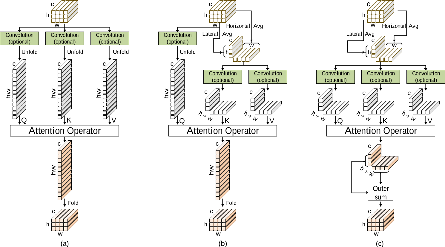
Figure 3. Illustrations of regular attention operator (a), KAO_$KV$ (b) and KAO_$QKV$ (c) on 2-D data. In the regular attention operator (a), the input tensor is unfolded into a mode-3 matrix and fed into the attention operator. The output of the attention operator is folded back to a tensor as the final output. In KAO_$KV$ (b), we juxtapose the horizontal and lateral average matrices derived from the input tensor as the key and value matrices. We keep the mode-3 unfolding of input tensor as the query matrix. In KAO_$QKV$ (c), all three input matrices use the juxtaposition of two average matrices. In contrast to KAO_$KV$, we use an outer-sum operation to generate the third-order tensor from the output of the attention operator.

Under this model, the marginal distributions of rows and columns are both multivariate normal (Allen and Tibshirani, 2010). Specifically, the $i$th row vector $\boldsymbol{X}_{i:}\in\mathbb{R}^{1\times w}$ follows $\boldsymbol{X}_{i:}^{T}\sim\mathcal{N}_{w}(\mu_{i}+\boldsymbol{\upsilon}^{T},\Omega_{ii}+\boldsymbol{\Psi})$, and the $j$th column vector $\boldsymbol{X}_{:j}\in\mathbb{R}^{h\times 1}$ follows $\boldsymbol{X}_{:j}\sim\mathcal{N}_{h}(\upsilon_{i}+\boldsymbol{\mu},\Psi_{ii}+\boldsymbol{\Omega})$. In the following discussion, we assume that $\boldsymbol{\Omega}$ and $\boldsymbol{\Psi}$ are diagonal, implying that any pair of variables in $\boldsymbol{X}$ are uncorrelated. Note that, although the variables in $\boldsymbol{X}$ are independent, their covariance matrix still follows the Kronecker covariance structure, thus capturing the relationships among rows and columns (Allen and Tibshirani, 2010; Wang et al., 2019).

3.3. Main Technical Results

Let $\overline{\boldsymbol{X}}_{row}=(\sum_{i=1}^{h}\boldsymbol{X}_{i:}^{T})/h\in\mathbb{R}^{w}$ and $\overline{\boldsymbol{X}}_{col}=(\sum_{j=1}^{w}\boldsymbol{X}_{:j})/w\in\mathbb{R}^{h}$ be the average of row and column vectors, respectively. Under the assumption above, $\overline{\boldsymbol{X}}_{row}$ and $\overline{\boldsymbol{X}}_{col}$ follow multivariate normal distributions as

(4) $$\overline{\boldsymbol{X}}_{row}\sim\mathcal{N}_{w}(\overline{\boldsymbol{\mu}}+\boldsymbol{\upsilon},\frac{\overline{\boldsymbol{\Omega}}+\boldsymbol{\Psi}}{h}),$$

(5) $$\overline{\boldsymbol{X}}_{col}\sim\mathcal{N}_{h}(\overline{\boldsymbol{\upsilon}}+\boldsymbol{\mu},\frac{\overline{\boldsymbol{\Psi}}+\boldsymbol{\Omega}}{w}),$$

where $\overline{\boldsymbol{\mu}}=(\sum_{i=1}^{h}\mu_{i})/h$, $\overline{\boldsymbol{\Omega}}=(\sum_{i=1}^{h}\Omega_{ii})/h$, $\overline{\boldsymbol{\upsilon}}=(\sum_{j=1}^{w}\upsilon_{j})/w$, and $\overline{\boldsymbol{\Psi}}=(\sum_{j=1}^{w}\Psi_{jj})/w$. Our main technical results can be summarized in the following theorem.

Theorem 1. Given the multivariate normal distributions in Eqs. (4) and (5) with diagonal $\boldsymbol{\Omega}$ and $\boldsymbol{\Psi}$, if (a) $\mathbf{r}_{1},\mathbf{r}_{2},\ldots,\mathbf{r}_{h}$ are independent and identically distributed (i.i.d.) random vectors that follow the distribution in Eq. (4), (b) $\mathbf{c}_{1},\mathbf{c}_{2},\ldots,\mathbf{c}_{w}$ are i.i.d. random vectors that follow the distribution in Eq. (5), (c) $\mathbf{r}_{1},\mathbf{r}_{2},\ldots,\mathbf{r}_{h}$ and $\mathbf{c}_{1},\mathbf{c}_{2},\ldots,\mathbf{c}_{w}$ are independent, we have

(6) $$\tilde{\boldsymbol{X}}\sim\mathcal{MN}_{h\times w}\left(\tilde{\boldsymbol{M}},\frac{\overline{\boldsymbol{\Psi}}+\boldsymbol{\Omega}}{w}\oplus\frac{\overline{\boldsymbol{\Omega}}+\boldsymbol{\Psi}}{h}\right),$$

where $\tilde{\boldsymbol{X}}=[\mathbf{r}_{1},\mathbf{r}_{2},\ldots,\mathbf{r}_{h}]^{T}+[\mathbf{c}_{1},\mathbf{c}_{2},\ldots,\mathbf{c}_{w}]$, $\tilde{\boldsymbol{M}}=(\boldsymbol{\mu}\diamondplus\boldsymbol{\upsilon})+(\overline{\boldsymbol{\mu}}+\overline{\boldsymbol{\upsilon}})$. In particular, if $h=w$, the covariance matrix satisfies

(7) $$\operatorname{tr}\left(\frac{\overline{\boldsymbol{\Psi}}+\boldsymbol{\Omega}}{w}\oplus\frac{\overline{\boldsymbol{\Omega}}+\boldsymbol{\Psi}}{h}\right)=\frac{2}{h}\operatorname{tr}\left(\boldsymbol{\Omega}\oplus\boldsymbol{\Psi}\right),$$

where $\operatorname{tr}(\cdot)$ denotes matrix trace.

Proof.

The fact that $\boldsymbol{\Omega}$ and $\boldsymbol{\Psi}$ are diagonal implies independence in the case of multivariate normal distributions. Therefore, it follows from assumptions (a) and (b) that

(8) $$[\mathbf{r}_{1},\mathbf{r}_{2},\ldots,\mathbf{r}_{h}]^{T}\sim\mathcal{MN}_{h\times w}\left(\boldsymbol{M}_{r},\boldsymbol{I}_{[h]}\otimes\frac{\overline{\boldsymbol{\Omega}}+\boldsymbol{\Psi}}{h}\right),$$

where $\boldsymbol{M}_{r}=\overline{\boldsymbol{\mu}}+[\boldsymbol{\upsilon},\boldsymbol{\upsilon},\ldots,\boldsymbol{\upsilon}]^{T}=\overline{\boldsymbol{\mu}}+\mathbf{1}_{[h]}\boldsymbol{\upsilon}^{T}$, and

(9) $$[\mathbf{c}_{1},\mathbf{c}_{2},\ldots,\mathbf{c}_{w}]\sim\mathcal{MN}_{h\times w}\left(\boldsymbol{M}_{c},\frac{\overline{\boldsymbol{\Psi}}+\boldsymbol{\Omega}}{w}\otimes\boldsymbol{I}_{[w]}\right),$$

where $\boldsymbol{M}_{c}=\overline{\boldsymbol{\upsilon}}+[\boldsymbol{\mu},\boldsymbol{\mu},\ldots,\boldsymbol{\mu}]=\overline{\boldsymbol{\upsilon}}+\boldsymbol{\mu}\mathbf{1}^{T}_{[w]}.$

Given assumption (c) and $\tilde{\boldsymbol{X}}=[\mathbf{r}_{1},\mathbf{r}_{2},\ldots,\mathbf{r}_{h}]^{T}+[\mathbf{c}_{1},\mathbf{c}_{2},\ldots,\mathbf{c}_{w}]$, we have

(10) $$\tilde{\boldsymbol{X}}\sim\mathcal{MN}_{h\times w}\left(\tilde{\boldsymbol{M}},\frac{\overline{\boldsymbol{\Psi}}+\boldsymbol{\Omega}}{w}\oplus\frac{\overline{\boldsymbol{\Omega}}+\boldsymbol{\Psi}}{h}\right),$$

where $\tilde{\boldsymbol{M}}=\boldsymbol{M}_{r}+\boldsymbol{M}_{c}=(\boldsymbol{\mu}\diamondplus\boldsymbol{\upsilon})+(\overline{\boldsymbol{\mu}}+\overline{\boldsymbol{\upsilon}})$.

If $h=w$, we have

(11) $$\operatorname{tr}(\boldsymbol{\Omega}\oplus\boldsymbol{\Psi})=h\left(\sum\Omega_{ii}+\sum\Psi_{jj}\right),$$

and

(12) $$\operatorname{tr}\left(\frac{\overline{\boldsymbol{\Psi}}+\boldsymbol{\Omega}}{w}\oplus\frac{\overline{\boldsymbol{\Omega}}+\boldsymbol{\Psi}}{h}\right)$$

$$= \operatorname{tr}\left(\frac{1}{h}(\boldsymbol{\Omega}\oplus\boldsymbol{\Psi})+\frac{1}{h}(\overline{\boldsymbol{\Psi}}+\overline{\boldsymbol{\Omega}})\right)$$

$$= \left(\sum\Omega_{ii}+\sum\Psi_{jj})+h(\overline{\boldsymbol{\Psi}}+\overline{\boldsymbol{\Omega}}\right)$$

$$= 2(\sum\Omega_{ii}+\sum\Psi_{jj})$$

$$= \frac{2}{h}\cdot\operatorname{tr}\left(\boldsymbol{\Omega}\oplus\boldsymbol{\Psi}\right).$$

This completes the proof of the theorem. ∎

With certain normalization on $\boldsymbol{X}$, we can have $\overline{\boldsymbol{\mu}}+\overline{\boldsymbol{\upsilon}}=0$, resulting in

(13) $$\tilde{\boldsymbol{M}}=\boldsymbol{\mu}\diamondplus\boldsymbol{\upsilon}.$$

As the trace of a covariance matrix measures the total variation, Theorem 1 implies that $\tilde{\boldsymbol{X}}$ follows a matrix-variate normal distribution with the same mean and scaled covariance as the distribution of $\boldsymbol{X}$ in Eq. (2). Given this conclusion and the process to obtain $\tilde{\boldsymbol{X}}$ from $\boldsymbol{X}$, we propose our Kronecker attention operators in the following section.

[]

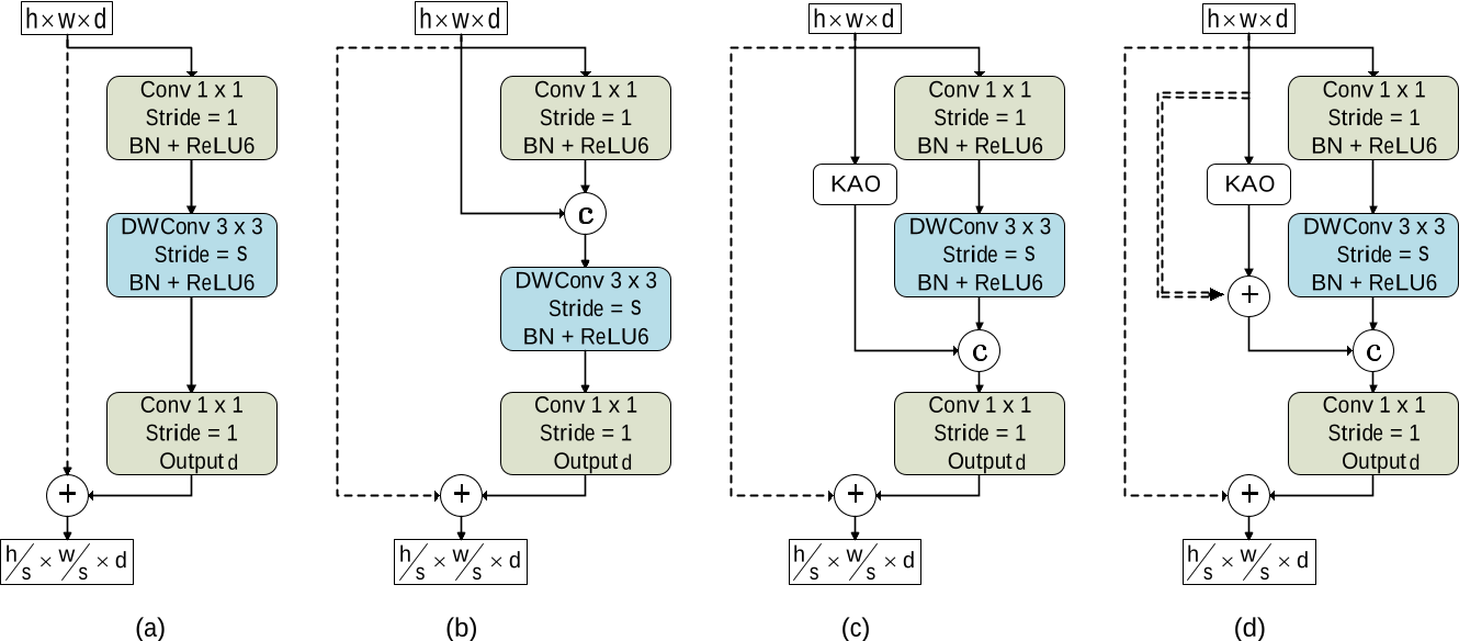
Figure 4. Architectures of the BaseModule (a), BaseSkipModule (b), AttnModule (c), and AttnSkipModule (d) as described in Section 3.5. The skip connections indicated by single dashed paths are not used when $s>1$ or $c\neq d$. Those indicated by double dashed paths are not used when $s>1$.

3.4. Kronecker Attention Operators

We describe the Kronecker attention operators (KAO) in the context of self-attention on 2-D data, but they can be easily generalized to generic attentions. In this case, the input to the $\ell$th layer is a third-order tensor $\boldsymbol{\mathscr{X}}^{(\ell)}\in\mathbb{R}^{h\times w\times c}$. Motivated by the theoretical results of Sections 3.2 and 3.3, we propose to use horizontal and lateral average matrices to represent original mode-3 unfolding without much information loss. Based on Eq. (4) and Eq. (5), the horizontal average matrix $\boldsymbol{H}$ and the lateral average matrix $\boldsymbol{L}$ are computed as

(14) $$\boldsymbol{H}=\frac{1}{h}\sum_{i=1}^{h}\boldsymbol{X}_{i::}^{(\ell)}\in\mathbb{R}^{w\times c},$$

$$\boldsymbol{L}=\frac{1}{w}\sum_{j=1}^{w}\boldsymbol{X}_{:j:}^{(\ell)}\in\mathbb{R}^{h\times c},$$

where $\boldsymbol{X}_{i::}^{(\ell)}$ and $\boldsymbol{X}_{:j:}^{(\ell)}$ are the horizontal and lateral slices (Kolda and Bader, 2009) of tensor $\boldsymbol{\mathscr{X}}^{(\ell)}$, respectively. We then form a matrix $\boldsymbol{C}$ by juxtaposing $\boldsymbol{H}^{T}$ and $\boldsymbol{L}^{T}$ as

(15) $$\boldsymbol{C}=[\boldsymbol{H}^{T},\boldsymbol{L}^{T}]\in\mathbb{R}^{c\times(h+w)}.$$

Based on the horizontal and lateral average matrices contained in $\boldsymbol{C}$, we propose two Kronecker attention operators (KAOs), i.e., KAO_$KV$ and KAO_$QKV$. In KAO_$KV$ as shown in Figure 3 (b), we use $\boldsymbol{X}_{(3)}^{(\ell)}$ as the query matrix and $\boldsymbol{C}$ as the key and value matrices as

(16) $$\boldsymbol{O}=\mbox{attn}(\boldsymbol{X}_{(3)}^{(\ell)},\boldsymbol{C},\boldsymbol{C})\in\mathbb{R}^{c\times hw}.$$

Note that the number of columns in $\boldsymbol{O}$ depends on the number of query vectors. Thus, we obtain $hw$ output vectors from the attention operation in Eq. (16). Similar to the regular attention operator, $\boldsymbol{O}$ is folded back to a third-order tensor $\boldsymbol{\mathscr{Y}}^{(\ell)}\in\mathbb{R}^{h\times w\times c}$ by considering the column vectors in $\boldsymbol{O}$ as mode-3 fibers of $\boldsymbol{\mathscr{Y}}^{(\ell)}$. KAO_$KV$ uses $\boldsymbol{\mathscr{Y}}^{(\ell)}$ as the output of layer $\ell$.

If $h=w$, the time and space complexities of KAO_$KV$ are $O(hw\times c\times(h+w))=O(h^{3}\times c)$ and $O(hw\times(h+w))=O(h^{3})$, respectively. Compared to the original local operator on 2-D data, KAO_$KV$ reduces time and space complexities by a factor of $h$.

In order to reduce the time and space complexities further, we propose another operator known as KAO_$QKV$. In KAO_$QKV$ as shown in Figure 3(c), we use $\boldsymbol{C}$ as the query, key, and value matrices as

(17) $$[\underbrace{\boldsymbol{\tilde{H}}}_{h},\underbrace{\boldsymbol{\tilde{L}}}_{w}]=\boldsymbol{O}=\mbox{attn}(\boldsymbol{C},\boldsymbol{C},\boldsymbol{C})\in\mathbb{R}^{c\times(h+w)}.$$

The final output tensor $\boldsymbol{\mathscr{Y}}^{(\ell)}\in\mathbb{R}^{h\times w\times c}$ is obtained as

(18) $$\boldsymbol{Y}^{(\ell)}_{::i}=\boldsymbol{\tilde{H}}^{T}_{i:}\diamondplus\boldsymbol{\tilde{L}}^{T}_{i:},$$

where $\boldsymbol{\tilde{H}}_{i:}$ and $\boldsymbol{\tilde{L}}_{i:}$ are the $i$th rows of the corresponding matrices. That is, the $i$th frontal slice of $\boldsymbol{\mathscr{Y}}^{(\ell)}$ is obtained by computing the outer sum of the $i$th rows of $\boldsymbol{\tilde{H}}$ and $\boldsymbol{\tilde{L}}$.

If $h=w$, the time and space complexities of KAO_$QKV$ are $O((h+w)\times c\times(h+w))=O(h^{2}\times c)$ and $O((h+w)\times(h+w))=O(h^{2})$, respectively. Thus, the time and space complexities have been reduced by a factor of $h^{2}$ as compared to the original local operator, and by a factor of $h$ as compared to KAO_$KV$.

Note that we do not consider linear transformations in our description, but these transformations can be applied to all three input matrices in KAO_$KV$ and KAO_$QKV$ as shown in Figure 3.

3.5. Kronecker Attention Modules and Networks

Table 1. Details of the KANets architecture. Each line describes a sequence of operators in the format of “input size / operator name / expansion rate $\boldsymbol{r}$ / number of output channels $\boldsymbol{c}$ / number of operators in the sequence $\boldsymbol{n}$ / stride $\boldsymbol{s}$”. “Conv2D” denotes the regular 2D convolutional layer. “AvgPool” and “FC” denote the global average pooling layer and the fully-connected layer, respectively. All depth-wise convolutions use the kernel size of $3\times 3$. For multiple operators in a sequence denoted in the same line, all operators produce $\boldsymbol{c}$ output channels. And the first operator applies the stride of $\boldsymbol{s}$ while the following operators applies the stride of 1. $k$ denotes the class number in the task.

Input	Operator	$\boldsymbol{r}$	$\boldsymbol{c}$	$\boldsymbol{n}$	$\boldsymbol{s}$
224${}^{2}\times$3	Conv2D $3\times 3$	-	32	1	2
112${}^{2}\times$32	BaseSkipModule	1	16	1	1
112${}^{2}\times$16	BaseSkipModule	6	24	2	2
56${}^{2}\times$24	BaseSkipModule	6	32	2	2
28${}^{2}\times$32	AttnSkipModule	6	32	1	1
28${}^{2}\times$32	BaseSkipModule	6	64	1	2
14${}^{2}\times$64	AttnSkipModule	6	64	3	1
14${}^{2}\times$64	AttnSkipModule	6	96	3	1
14${}^{2}\times$96	BaseSkipModule	6	160	1	2
7${}^{2}\times$160	AttnSkipModule	6	160	2	1
7${}^{2}\times$160	AttnSkipModule	6	320	1	1
7${}^{2}\times$320	Conv2D $1\times 1$	-	1280	1	1
7${}^{2}\times$1280	AvgPool + FC	-	$k$	1	-

Attention models have not been used in compact deep models to date, primarily due to their high computational cost. Our efficient KAOs make it possible to use attention operators in compact convolutional neural networks (CNNs) like MobileNet (Sandler et al., 2018). In this section, we design a family of efficient Kronecker attention modules based on MobileNetV2 that can be used in compact CNNs.

BaseModule: MobileNetV2 (Sandler et al., 2018) is mainly composed of bottleneck blocks with inverted residuals. Each bottleneck block consists of three convolutional layers; those are, $1\times 1$ convolutional layer, $3\times 3$ depth-wise convolutional layer, and another $1\times 1$ convolutional layer. Suppose the expansion factor is $r$ and stride is $s$. Given input $\boldsymbol{\mathscr{X}}^{(\ell)}\in\mathbb{R}^{h\times w\times c}$ for the $\ell$th block, the first $1\times 1$ convolutional layer outputs $rc$ feature maps $\boldsymbol{\mathscr{\tilde{X}}}^{(\ell)}\in\mathbb{R}^{h\times w\times rc}$. The depth-wise convolutional layer uses a stride of $s$ and outputs $rc$ feature maps $\boldsymbol{\mathscr{\bar{X}}}^{(\ell)}\in\mathbb{R}^{\frac{h}{s}\times\frac{w}{s}\times rc}$. The last $1\times 1$ convolutional layer produces $d$ feature maps $\boldsymbol{\mathscr{Y}}^{(\ell)}\in\mathbb{R}^{\frac{h}{s}\times\frac{w}{s}\times d}$. When $s=1$ and $c=d$, a skip connection is added between $\boldsymbol{\mathscr{X}}^{(\ell)}$ and $\boldsymbol{\mathscr{Y}}^{(\ell)}$. The BaseModule is illustrated in Figure 4 (a).

BaseSkipModule: To facilitate feature reuse and gradient back-propagation in deep models, we improve the BaseModule by adding a skip connection. Given input $\boldsymbol{\mathscr{X}}^{(\ell)}$, we use an expansion factor of $r-1$ for the first $1\times 1$ convolutional layer, instead of $r$ as in BaseModule. We then concatenate the output with the original input, resulting in $\boldsymbol{\mathscr{\tilde{X}}}^{(\ell)}\in\mathbb{R}^{h\times w\times rc}$. The other parts of the BaseSkipModule are the same as those of the BaseModule as illustrated in Figure 4 (b). Compared to the BaseModule, the BaseSkipModule reduces the number of parameters by $c\times c$ and computational cost by $h\times w\times c$. It achieves better feature reuse and gradient back-propagation.

AttnModule: We propose to add an attention operator into the BaseModule to enable the capture of global features. We reduce the expansion factor of the BaseModule by $1$ and add a new parallel path with an attention operator that outputs $c$ feature maps. Concretely, after the depth-wise convolutional layer, the original path outputs $\boldsymbol{\mathscr{\bar{X}}}^{(\ell)}_{a}\in\mathbb{R}^{\frac{h}{s}\times\frac{w}{s}\times(r-1)c}$. The attention operator, optionally followed by an average pooling of stride $s$ if $s>1$, produces $\boldsymbol{\mathscr{\bar{X}}}^{(\ell)}_{b}\in\mathbb{R}^{\frac{h}{s}\times\frac{w}{s}\times c}$. Concatenating them gives $\boldsymbol{\mathscr{\bar{X}}}^{(\ell)}\in\mathbb{R}^{\frac{h}{s}\times\frac{w}{s}\times rc}$. The final $1\times 1$ convolutional layer remains the same. Within the attention operator, we only apply the linear transformation on the value matrix $\boldsymbol{V}$ to limit the number of parameters and required computational resources. We denote this module as the AttnModule as shown in Figure 4 (b). In this module, the original path acts as locality-based feature extractors, while the new parallel path with an attention operator computes global features. This enables the module to incorporate both local and global information. Note that we can use any attention operator in this module, including the regular attention operator and our KAOs.

AttnSkipModule: We propose to add an additional skip connection in the AttnModule, as shown in Figure 4 (d). This skip connection can always be added unless $s>1$. The AttnSkipModule has the same amount of parameters and computational cost as the AttnModule.

4. Experimental Studies

In this section, we evaluate our proposed operators and networks on image classification and segmentation tasks. We first compare our proposed KAOs with regular attention operators in terms of computational cost and memory usage. Next, we design novel compact CNNs known as Kronecker attention networks (KANets) using our proposed operators and modules. We compare KANets with other compact CNNs on the ImageNet ILSVRC 2012 dataset (Deng et al., 2009). Ablation studies are conducted to investigate how our KAOs benefit the entire networks. We also perform experiments on the PASCAL 2012 dataset (Everingham et al., 2010) to show the effectiveness of our KAOs on general application scenarios.

Table 2. Comparisons between the regular attention operator, the regular attention operator with a pooling operation (Wang et al., 2018), and our proposed KAO_$KV$ and KAO_$QKV$ in terms of the number of parameters, number of MAdd, memory usage, and CPU inference time on simulated data of different sizes. The input sizes are given in the format of “batch size $\times$ spatial sizes $\times$ number of input channels”. “Attn” denotes the regular attention operator. “Attn+Pool” denotes the regular attention operator which employs a $2\times 2$ pooling operation on $\boldsymbol{K}$ and $\boldsymbol{V}$ input matrices to reduce required computational resources.

Input	Operator	MAdd	Cost Saving	Memory	Memory Saving	Time	Speedup
$8\times 14^{2}\times 8$	Attn	0.63m	0.00%	5.2MB	0.00%	5.8ms	1.0$\times$
	Attn+Pool	0.16m	75.00%	1.5MB	71.65%	2.0ms	3.0$\times$
	KAO$KV$	0.09m	85.71%	0.9MB	82.03%	1.7ms	3.5$\times$
	KAO$QKV$	0.01m	97.71%	0.3MB	95.06%	0.8ms	6.8$\times$
$8\times 28^{2}\times 8$	Attn	9.88m	0.00%	79.9MB	0.00%	72.4ms	1.0$\times$
	Attn+Pool	2.47m	75.00%	20.7MB	74.13%	20.9ms	3.5$\times$
	KAO$KV$	0.71m	92.86%	6.5MB	91.88%	7.1ms	10.1$\times$
	KAO$QKV$	0.05m	99.46%	0.9MB	98.85%	1.7ms	40.9$\times$
$8\times 56^{2}\times 8$	Attn	157.55m	0.00%	1,262.6MB	0.00%	1,541.1ms	1.0$\times$
	Attn+Pool	39.39m	75.00%	318.7MB	74.76%	396.9ms	3.9$\times$
	KAO$KV$	5.62m	96.43%	48.2MB	96.18%	49.6ms	31.1$\times$
	KAO$QKV$	0.21m	99.87%	3.4MB	99.73%	5.1ms	305.8$\times$

4.1. Experimental Setup

In this section, we describe the experimental setups for both image classification tasks and image segmentation tasks.

Experimental Setup for Image Classification As a common practice on this dataset, we use the same data augmentation scheme in He et al. (2016). Specifically, during training, we scale each image to $256\times 256$ and then randomly crop a $224\times 224$ patch. During inference, the center-cropped patches are used. We train our KANets using the same settings as MobileNetV2 (Sandler et al., 2018) with minor changes. We perform batch normalization (Ioffe and Szegedy, 2015) on the coefficient matrices in KAOs to stabilize the training. All trainable parameters are initialized with the Xavier initialization (Glorot and Bengio, 2010). We use the standard stochastic gradient descent optimizer with a momentum of 0.9 (Sutskever et al., 2013) to train models for 150 epochs in total. The initial learning rate is 0.1 and it decays by 0.1 at the $80$th, $105$th, and $120$th epoch. Dropout (Srivastava et al., 2014) with a keep rate of $0.8$ is applied after the global average pooling layer. We use 8 TITAN Xp GPUs and a batch size of $512$ for training, which takes about $1.5$ days. Since labels of the test dataset are not available, we train our networks on training dataset and report accuracies on the validation dataset.

Experimental Setup for Image Segmentation We train all the models with randomly cropped patches of size $321\times 321$ and a batch size of 8. Data augmentation by randomly scaling the inputs for training is employed. We adopt the “poly” learning rate policy (Liu et al., 2015) with $power=0.9$, and set the initial learning rate to 0.00025. Following DeepLabV2, we use the ResNet-101 model pre-trained on ImageNet (Deng et al., 2009) and MS-COCO (Lin et al., 2014) for initialization. The models are then trained for 25,000 iterations with a momentum of 0.9 and a weight decay of 0.0005. We perform no post-processing such as conditional random fields and do not use multi-scale inputs due to limited GPU memory. All the models are trained on the training set and evaluated on the validation set.

4.2. Comparison of Computational Efficiency

According to the theoretical analysis in Section 3.4, our KAOs have efficiency advantages over regular attention operators on high-order data, especially for inputs with large spatial sizes. We conduct simulated experiments to evaluate the theoretical results. To reduce the influence of external factors, we build networks composed of a single attention operator, and apply the TensorFlow profile tool (Abadi et al., 2016) to report the multiply-adds (MAdd), required memory, and time consumed on 2-D simulated data. For the simulated input data, we set the batch size and number of channels both to 8, and test three spatial sizes; those are, $56\times 56$, $28\times 28$, and $14\times 14$. The number of output channels is also set to 8.

Table 2 summarizes the comparison results. On simulated data of spatial sizes $56\times 56$, our KAO_$KV$ and KAO_$QKV$ achieve 31.1 and 305.8 times speedup, and 96.18% and 99.73% memory saving compared to the regular attention operator, respectively. Our proposed KAOs show significant improvements over regular attention operators in terms of computational resources, which is consistent with the theoretical analysis. In particular, the amount of improvement increases as the spatial sizes increase. These results show that the proposed KAOs are efficient attention operators on high-dimensional and high-order data.

Table 3. Comparisons between KANets and other CNNs in terms of the top-1 accuracy on the ImageNet validation set, the number of total parameters, and MAdd. We use KANet_$KV$ and KANet_$QKV$ to denote KANets using KAO_$KV$ and KAO_$QKV$, respectively.

Model	Top-1	Params	MAdd
GoogleNet	0.698	6.8m	1550m
VGG16	0.715	128m	15300m
AlexNet	0.572	60m	720m
SqueezeNet	0.575	1.3m	833m
MobileNetV1	0.706	4.2m	569m
ShuffleNet 1.5x	0.715	3.4m	292m
ChannelNet-v1	0.705	3.7m	407m
MobileNetV2	0.720	3.47m	300m
KANet$\boldsymbol{KV}$ (ours)	0.729	3.44m	288m
KANet$\boldsymbol{QKV}$ (ours)	0.728	3.44m	281m

4.3. Results on Image Classification

With the high efficiency of our KAOs, we have proposed several efficient Kronecker attention modules for compact CNNs in Section 3.5. To further show the effectiveness of KAOs and the modules, we build novel compact CNNs known as Kronecker attention networks (KANets). Following the practices in (Wang et al., 2018), we apply these modules on inputs of spatial sizes $28\times 28$, $14\times 14$, and $7\times 7$. The detailed network architecture is described in Table 1 in the Section 4.1.

We compare KANets with other CNNs on the ImageNet ILSVRC 2012 image classification dataset, which serves as the benchmark for compact CNNs (Howard et al., 2017; Zhang et al., 2017; Gao et al., 2018a; Sandler et al., 2018). The dataset contains 1.2 million training, 50 thousand validation, and 50 thousand testing images. Each image is labeled with one of 1,000 classes. Details of the experimental setups are provided in the Section 4.1.

The comparison results between our KANets and other CNNs in terms of the top-1 accuracy, number of parameters, and MAdd are reported in Table 3. SqueezeNet (Iandola et al., 2016) has the least number of parameters, but uses the most MAdd and does not obtain competitive performance as compared to other compact CNNs. Among compact CNNs, MobileNetV2 (Sandler et al., 2018) is the previous state-of-the-art model, which achieves the best trade-off between effectiveness and efficiency. According to the results, our KANets significantly outperform MobileNetV2 with 0.03 million fewer parameters. Specifically, our KANet_$KV$ and KANet_$QKV$ outperform MobileNetV2 by margins of 0.9% and 0.8%, respectively. More importantly, our KANets has the least computational cost. These results demonstrate the effectiveness and efficiency of our proposed KAOs.

The performance of KANets indicates that our proposed methods are promising, since we only make small modifications to the architecture of MobileNetV2 to include KAOs. Compared to modules with the regular convolutional layers only, our proposed modules with KAOs achieve better performance without using excessive computational resources. Thus, our methods can be used widely for designing compact deep models. Our KAOs successfully address the practical challenge of applying regular attention operators on high-order data. In the next experiments, we show that our proposed KAOs are as effective as regular attention operators.

Table 4. Comparisons between KANets with regular attention operators (denoted as AttnNet), KANets with regular attention operators with a pooling operation (denoted as AttnNet+Pool) and KANets with KAOs in terms of the top-1 accuracy on the ImageNet validation set, the number of total parameters, and MAdd.

Model	Top-1	Params	MAdd
AttnNet	0.730	3.44m	365m
AttnNet+Pool	0.729	3.44m	300m
KANet$KV$	0.729	3.44m	288m
KANet$QKV$	0.728	3.44m	281m

4.4. Comparison with Regular Attention Operators

We perform experiments to compare our proposed KAOs with regular attention operators. We consider the regular attention operator and the one with a pooling operation in (Wang et al., 2018). For the attention operator with pooling operation, the spatial sizes of the key matrix $\boldsymbol{K}$ and value matrix $\boldsymbol{V}$ are reduced by $2\times 2$ pooling operations to save computation cost. To compare these operators in fair settings, we replace all KAOs in KANets with regular attention operators and regular attention operators with a pooling operation, denoted as AttnNet and AttnNet+Pool, respectively.

The comparison results are summarized in Table 4. Note that all these models have the same number of parameters. We can see that KANet_$KV$ and KANet_$QKV$ achieve similar performance as AttnNet and AttnNet+Pool with dramatic reductions of computational cost. The results indicate that our proposed KAOs are as effective as regular attention operators while being much more efficient. In addition, our KAOs are better than regular attention operators that uses a pooling operation to increase efficiency in (Wang et al., 2018).

4.5. Ablation Studies

To show how our KAOs benefit entire networks in different settings, we conduct ablation studies on MobileNetV2 and KANet_$KV$. For MobileNetV2, we replace BaseModules with AttnModules as described in Section 3.5, resulting in a new model denoted as MobileNetV2+KAO. On the contrary, based on KANet_$KV$, we replace all AttnSkipModules by BaseModules. The resulting model is denoted as KANet w/o KAO.

Table 5 reports the comparison results. By employing KAO_$KV$, MobileNetV2+KAO gains a performance boost of 0.6% with fewer parameters than MobileNetV2. On the other hand, KANet_$KV$ outperforms KANet w/o KAO by a margin of 0.8%, while KANet w/o KAO has more parameters than KANet_$KV$. KANet_$KV$ achieves the best performance while costing the least computational resources. The results indicate that our proposed KAOs are effective and efficient, which is independent of specific network architectures.

Table 5. Comparisons between MobileNetV2, MobileNetV2 with KAOs_$KV$ (denoted as MobileNetV2+KAO_$KV$), KANet_$KV$, and KANet_$KV$ without KAO_$KV$ (denoted as KANet w/o KAO) in terms of the top-1 accuracy on the ImageNet validation set, the number of total parameters, and MAdd.

Model	Top-1	Params	MAdd
MobileNetV2	0.720	3.47m	300m
MobileNetV2+KAO	0.726	3.46m	298m
KANet$KV$	0.729	3.44m	288m
KANet w/o KAO	0.721	3.46m	298m

4.6. Results on Image Segmentation

Table 6. Comparisons of DeepLabV2, DeepLabV2 with the regular attention operator (DeepLabV2+Attn), DeepLabV2 with our KAO_$KV$ (DeepLabV2+KAO_$KV$), and DeepLabV2 with our KAO_$QKV$ (DeepLabV2+KAO_$QKV$) in terms of the pixel-wise accuracy, and mean IOU on the PASCAL VOC 2012 validation dataset.

Model	Accuracy	Mean IOU
DeepLabV2	0.944	75.1
DeepLabV2+Attn	0.947	76.3
DeepLabV2+KAO$KV$	0.946	75.9
DeepLabV2+KAO$QKV$	0.946	75.8

In order to show the efficiency and effectiveness of our KAOs in broader application scenarios, we perform additional experiments on image segmentation tasks using the PASCAL 2012 dataset (Everingham et al., 2010). With the extra annotations provided by (Hariharan et al., 2011), the augmented dataset contains 10,582 training, 1,449 validation, and 1,456 testing images. Each pixel of the images is labeled by one of 21 classes with 20 foreground classes and 1 background class.

We re-implement the DeepLabV2 model (Chen et al., 2018) as our baseline. Following (Wang and Ji, 2018), using attention operators as the output layer, instead of atrous spatial pyramid pooling (ASPP), results in a significant performance improvement. In our experiments, we replace ASPP with the regular attention operator and our proposed KAOs, respectively, and compare the results. For all attention operators, linear transformations are applied on $\boldsymbol{Q}$, $\boldsymbol{K}$, and $\boldsymbol{V}$. Details of the experimental setups are provided in the Section 4.1.

Table 6 shows the evaluation results in terms of pixel accuracy and mean intersection over union (IoU) on the PASCAL VOC 2012 validation set. Clearly, models with attention operators outperform the baseline model with ASPP. Compared with the regular attention operator, KAOs result in similar pixel-wise accuracy but slightly lower mean IoU. From the pixel-wise accuracy, results indicate that KAOs are as effective as the regular attention operator. The decrease in mean IoU may be caused by the strong structural assumption behind KAOs. Overall, the experimental results demonstrate the efficiency and effectiveness of our KAOs in broader application scenarios.

5. Conclusions

In this work, we propose Kronecker attention operators to address the practical challenge of applying attention operators on high-order data. We investigate the problem from a probabilistic perspective and use matrix-variate normal distributions with Kronecker covariance structure. Experimental results show that our KAOs reduce the amount of required computational resources by a factor of hundreds, with larger factors for higher-dimensional and higher-order data. We employ KAOs to design a family of efficient modules, leading to our KANets. KANets significantly outperform the previous state-of-the-art compact models on image classification tasks, with fewer parameters and less computational cost. Additionally, we perform experiments on the image segmentation task to show the effectiveness of our KAOs on general application scenarios.

- (1)
- Abadi et al. (2016) Martín Abadi, Paul Barham, Jianmin Chen, Zhifeng Chen, Andy Davis, Jeffrey Dean, Matthieu Devin, Sanjay Ghemawat, Geoffrey Irving, Michael Isard, et al. 2016. Tensorflow: a system for large-scale machine learning.. In OSDI, Vol. 16. 265–283.
- Allen and Tibshirani (2010) Genevera I Allen and Robert Tibshirani. 2010. Transposable regularized covariance models with an application to missing data imputation. The Annals of Applied Statistics 4, 2 (2010), 764.
- Bahdanau et al. (2015) Dzmitry Bahdanau, Kyunghyun Cho, and Yoshua Bengio. 2015. Neural machine translation by jointly learning to align and translate. International Conference on Learning Representations (2015).
- Chen et al. (2018) Liang-Chieh Chen, George Papandreou, Iasonas Kokkinos, Kevin Murphy, and Alan L Yuille. 2018. Deeplab: Semantic image segmentation with deep convolutional nets, atrous convolution, and fully connected crfs. IEEE transactions on pattern analysis and machine intelligence 40, 4 (2018), 834–848.
- Deng et al. (2009) J. Deng, W. Dong, R. Socher, L.-J. Li, K. Li, and L. Fei-Fei. 2009. ImageNet: A Large-Scale Hierarchical Image Database. In Proceedings of the IEEE Conference on Computer Vision and Pattern Recognition.
- Everingham et al. (2010) Mark Everingham, Luc Van Gool, Christopher KI Williams, John Winn, and Andrew Zisserman. 2010. The pascal visual object classes (voc) challenge. International journal of computer vision 88, 2 (2010), 303–338.
- Gao and Ji (2019) Hongyang Gao and Shuiwang Ji. 2019. Graph representation learning via hard and channel-wise attention networks. In Proceedings of the 25th ACM SIGKDD International Conference on Knowledge Discovery & Data Mining. 741–749.
- Gao et al. (2018a) Hongyang Gao, Zhengyang Wang, and Shuiwang Ji. 2018a. ChannelNets: Compact and Efficient Convolutional Neural Networks via Channel-Wise Convolutions. In Advances in Neural Information Processing Systems. 5203–5211.
- Gao et al. (2018b) Hongyang Gao, Zhengyang Wang, and Shuiwang Ji. 2018b. Large-scale learnable graph convolutional networks. In Proceedings of the 24th ACM SIGKDD International Conference on Knowledge Discovery & Data Mining. 1416–1424.
- Glorot and Bengio (2010) Xavier Glorot and Yoshua Bengio. 2010. Understanding the difficulty of training deep feedforward neural networks. In Proceedings of the Thirteenth International Conference on Artificial Intelligence and Statistics. 249–256.
- Graham (2018) Alexander Graham. 2018. Kronecker products and matrix calculus with applications. Courier Dover Publications.
- Gupta and Nagar (2018) Arjun K Gupta and Daya K Nagar. 2018. Matrix variate distributions. Chapman and Hall/CRC.
- Hariharan et al. (2011) Bharath Hariharan, Pablo Arbeláez, Lubomir Bourdev, Subhransu Maji, and Jitendra Malik. 2011. Semantic contours from inverse detectors. In Computer Vision (ICCV), 2011 IEEE International Conference on. IEEE, 991–998.
- He et al. (2016) Kaiming He, Xiangyu Zhang, Shaoqing Ren, and Jian Sun. 2016. Deep residual learning for image recognition. In Proceedings of the IEEE conference on computer vision and pattern recognition. 770–778.
- Howard et al. (2017) Andrew G Howard, Menglong Zhu, Bo Chen, Dmitry Kalenichenko, Weijun Wang, Tobias Weyand, Marco Andreetto, and Hartwig Adam. 2017. Mobilenets: Efficient convolutional neural networks for mobile vision applications. arXiv preprint arXiv:1704.04861 (2017).
- Huang et al. (2018) Zilong Huang, Xinggang Wang, Lichao Huang, Chang Huang, Yunchao Wei, and Wenyu Liu. 2018. CCNet: Criss-Cross Attention for Semantic Segmentation. arXiv preprint arXiv:1811.11721 (2018).
- Iandola et al. (2016) Forrest N Iandola, Song Han, Matthew W Moskewicz, Khalid Ashraf, William J Dally, and Kurt Keutzer. 2016. SqueezeNet: AlexNet-level accuracy with 50x fewer parameters and¡ 0.5 MB model size. arXiv preprint arXiv:1602.07360 (2016).
- Ioffe and Szegedy (2015) Sergey Ioffe and Christian Szegedy. 2015. Batch Normalization: Accelerating Deep Network Training by Reducing Internal Covariate Shift. In International Conference on Machine Learning. 448–456.
- Johnson and Zhang (2015) Rie Johnson and Tong Zhang. 2015. Semi-supervised convolutional neural networks for text categorization via region embedding. In Advances in neural information processing systems. 919–927.
- Kalaitzis et al. (2013) Alfredo Kalaitzis, John Lafferty, Neil Lawrence, and Shuheng Zhou. 2013. The bigraphical lasso. In International Conference on Machine Learning. 1229–1237.
- Kolda and Bader (2009) Tamara G. Kolda and Brett W. Bader. 2009. Tensor Decompositions and Applications. SIAM Rev. 51, 3 (2009), 455–500.
- LeCun et al. (1998) Yann LeCun, Léon Bottou, Yoshua Bengio, and Patrick Haffner. 1998. Gradient-based learning applied to document recognition. Proc. IEEE 86, 11 (1998), 2278–2324.
- Li et al. (2018) Guanbin Li, Xiang He, Wei Zhang, Huiyou Chang, Le Dong, and Liang Lin. 2018. Non-locally Enhanced Encoder-Decoder Network for Single Image De-raining. In 2018 ACM Multimedia Conference on Multimedia Conference. ACM, 1056–1064.
- Lin et al. (2014) Tsung-Yi Lin, Michael Maire, Serge Belongie, James Hays, Pietro Perona, Deva Ramanan, Piotr Dollár, and C Lawrence Zitnick. 2014. Microsoft coco: Common objects in context. In European conference on computer vision. Springer, 740–755.
- Liu et al. (2015) Wei Liu, Andrew Rabinovich, and Alexander C Berg. 2015. Parsenet: Looking wider to see better. arXiv preprint arXiv:1506.04579 (2015).
- Lu et al. (2016) Jiasen Lu, Jianwei Yang, Dhruv Batra, and Devi Parikh. 2016. Hierarchical question-image co-attention for visual question answering. In Advances In Neural Information Processing Systems. 289–297.
- Malinowski et al. (2018) Mateusz Malinowski, Carl Doersch, Adam Santoro, and Peter Battaglia. 2018. Learning Visual Question Answering by Bootstrapping Hard Attention. In Proceedings of the European Conference on Computer Vision (ECCV). 3–20.
- Sandler et al. (2018) Mark Sandler, Andrew Howard, Menglong Zhu, Andrey Zhmoginov, and Liang-Chieh Chen. 2018. Mobilenetv2: Inverted residuals and linear bottlenecks. In 2018 IEEE/CVF Conference on Computer Vision and Pattern Recognition. IEEE, 4510–4520.
- Srivastava et al. (2014) Nitish Srivastava, Geoffrey Hinton, Alex Krizhevsky, Ilya Sutskever, and Ruslan Salakhutdinov. 2014. Dropout: A simple way to prevent neural networks from overfitting. Journal of Machine Learning Research 15, 1 (2014), 1929–1958.
- Sutskever et al. (2013) Ilya Sutskever, James Martens, George Dahl, and Geoffrey Hinton. 2013. On the importance of initialization and momentum in deep learning. In International conference on machine learning. 1139–1147.
- Ulyanov et al. (2016) Dmitry Ulyanov, Andrea Vedaldi, and Victor Lempitsky. 2016. Instance Normalization: The Missing Ingredient for Fast Stylization. arXiv preprint arXiv:1607.08022 (2016).
- Van Loan (2000) Charles F Van Loan. 2000. The ubiquitous Kronecker product. Journal of computational and applied mathematics 123, 1-2 (2000), 85–100.
- Vaswani et al. (2017) Ashish Vaswani, Noam Shazeer, Niki Parmar, Jakob Uszkoreit, Llion Jones, Aidan N Gomez, Łukasz Kaiser, and Illia Polosukhin. 2017. Attention is all you need. In Advances in Neural Information Processing Systems. 5998–6008.
- Veličković et al. (2017) Petar Veličković, Guillem Cucurull, Arantxa Casanova, Adriana Romero, Pietro Liò, and Yoshua Bengio. 2017. Graph Attention Networks. arXiv preprint arXiv:1710.10903 (2017).
- Wang et al. (2018) Xiaolong Wang, Ross Girshick, Abhinav Gupta, and Kaiming He. 2018. Non-local neural networks. In The IEEE Conference on Computer Vision and Pattern Recognition (CVPR), Vol. 1. 4.
- Wang and Ji (2018) Zhengyang Wang and Shuiwang Ji. 2018. Smoothed Dilated Convolutions for Improved Dense Prediction. In Proceedings of the 24th ACM SIGKDD International Conference on Knowledge Discovery & Data Mining. ACM, 2486–2495.
- Wang et al. (2019) Zhengyang Wang, Hao Yuan, and Shuiwang Ji. 2019. Spatial Variational Auto-Encoding via Matrix-Variate Normal Distributions. In Proceedings of the 2019 SIAM International Conference on Data Mining. SIAM, 648–656.
- Xu et al. (2015) Kelvin Xu, Jimmy Ba, Ryan Kiros, Kyunghyun Cho, Aaron Courville, Ruslan Salakhudinov, Rich Zemel, and Yoshua Bengio. 2015. Show, attend and tell: Neural image caption generation with visual attention. In International conference on machine learning. 2048–2057.
- Zhang et al. (2017) Xiangyu Zhang, Xinyu Zhou, Mengxiao Lin, and Jian Sun. 2017. Shufflenet: An extremely efficient convolutional neural network for mobile devices. arXiv preprint arXiv:1707.01083 (2017).
- Zhao et al. (2018) Hengshuang Zhao, Yi Zhang, Shu Liu, Jianping Shi, Chen Change Loy, Dahua Lin, and Jiaya Jia. 2018. PSANet: Point-wise Spatial Attention Network for Scene Parsing. In Proceedings of the European Conference on Computer Vision (ECCV). 267–283.