Nucleon polarizabilities in covariant baryon chiral perturbation theory with explicit $\Delta$ degrees of freedom

Abstract

We compute various nucleon polarizabilities in chiral perturbation theory implementing the $\Delta$-full ($\Delta$-less) approach up to order $\epsilon^{3}+q^{4}$ ($q^{4}$) in the small-scale (chiral) expansion. The calculation is carried out using the covariant formulation of $\chi$PT by utilizing the extended on-mass shell renormalization scheme. Except for the spin-independent dipole polarizabilities used to fix the values of certain low-energy constants, our results for the nucleon polarizabilities are pure predictions. We compare our calculations with available experimental data and other theoretical results. The importance of the explicit treatment of the $\Delta$ degree of freedom in the effective field theory description of the nucleon polarizabilities is analyzed. We also study the convergence of the $1/m$ expansion and analyze the efficiency of the heavy-baryon approach for the nucleon polarizabilities.

I Introduction

Understanding the structure of the nucleon is one of the key challenges in the physics of strong interactions, and quantum chromodynamics (QCD) in particular. One of the most direct ways to access the nucleon structure is to use electromagnetic probes. In the present work we focus on the nucleon polarizabilites, which characterize the (second-order) response of the nucleon to an applied electromagnetic field. In recent decades, the nucleon polarizabilites have been intensively studied both experimentally and theoretically. At the moment, the dipole scalar (spin-independent) polarizabilites of both the proton and the neutron are determined fairly well by various methods Tanabashi et al. (2018) as well as the forward and backward spin polarizabilites of the proton Ahrens et al. (2001); Dutz et al. (2003); Camen et al. (2002). Recent measurements of double-polarized Compton scattering at the Mainz Microtron allowed one to extract also other proton spin polarizabilites Martel et al. (2015); Paudyal et al. (2019).

There are also experimental results for some of the generalized ($Q^{2}$-dependent) polarizabilites of the proton and the neutron Prok et al. (2009); Amarian et al. (2004); Guler et al. (2015); Gryniuk et al. (2016); Deur (2019).

From the theoretical side, a significant progress has been made using lattice simulations Detmold et al. (2010); Hall et al. (2014); Lujan et al. (2014); Freeman et al. (2014); Chang et al. (2015); Bignell et al. (2017, 2018), i.e. by directly solving QCD in the non-perturbative regime on a discrete Euclidean space-time grid. However, one is not yet in the position to perform an accurate determination of the nucleon polarizabilites calculated on the lattice for physical pion masses.

Another systematic theoretical approach is provided by effective field theories, in particular, by chiral perturbation theory ($\chi$PT), see Bernard et al. (1991, 1992) for pioneering studies of the nucleon’s electromagnetic polarizabilities in this framework. Chiral perturbation theory is an effective field theory of the standard model consistent with its symmetries and the ways they are broken. It allows one to expand hadronic observables in powers of the small parameter $q$ defined as the ratio of the typical soft scales such as the pion mass $M$ and external-particle 3-momenta $|\vec{p}|$ and the hard scale $\Lambda_{\rm b}$ of the order of the $\rho$-meson mass. The effective chiral Lagrangian is expanded in powers of derivatives and the pion mass. In the nucleon sector, an additional complication arises due to the presence of an extra mass scale, namely the nucleon mass, which can potentially break the power counting. One way to circumvent this problem is to perform the $1/m$ expansion on the level of the effective Lagrangian. This leads to the so-called heavy-baryon approach. The heavy-baryon scheme has been intensively used for the analysis of many hadronic reactions including the nucleon Compton scattering (and, therefore, nucleon polarizabilites), see e.g. Bernard et al. (1995); Vijaya Kumar et al. (2000); Gellas et al. (2000); Hemmert et al. (1997) and Bernard et al. (1995); Bernard (2008) for review articles. The heavy-baryon expansion is, however, known to violate certain analytic properties of the $S$-matrix Becher and Leutwyler (1999), which may lead to a slower convergence of the chiral expansion. This feature has also been observed in the actual calculations of the nucleon polarizabilites.

An alternative approach to processes involving nucleons consists in keeping the covariant structure of the effective Lagrangian and absorbing the power-counting breaking terms by a redefinition of the lower order low-energy constants Becher and Leutwyler (1999); Fuchs et al. (2003). In this work, we adopt a version of the covariant approach known as the extended on-mass-shell renormalization scheme (EOMS) Gegelia and Japaridze (1999); Fuchs et al. (2003). When necessary, we will slightly modify this scheme in order to enable a direct comparison to the heavy-baryon results (see e.g. Siemens et al. (2016)).

Another obstacle for the rapid convergence of the chiral expansion in the single-nucleon systems is the presence of the $\Delta$(1232)-resonance that is located close to the pion-nucleon threshold and is known to strongly couple to the pion-nucleon channel. This introduces another small scale $\Delta\equiv m_{\Delta}-m\approx 2\,M$, which leads to the appearance of terms of order $\mathcal{O}(M/\Delta)$ in the expansion of observables. A natural way to improve this situation is to include the $\Delta$-isobar field explicitly into the effective Lagrangian. We follow here the so-called small-scale-expansion (SSE) scheme by treating the scale $\Delta$ on the same footing as $M$ or $|\vec{p}|$ Hemmert et al. (1998). The universal expansion parameter is then called $\epsilon$. For recent applications of this theoretical approach to various processes in the single-nucleon sector see Bernard et al. (2013); Yao et al. (2016); Siemens et al. (2017); Rijneveen et al. (2020). In this work, we compare the efficiency and convergence of both the $\Delta$-full and $\Delta$-less schemes by calculating various nucleon polarizabilites up to orders $\epsilon^{3}+q^{4}$ and $q^{4}$, respectively. Our analysis is particularly instructive since we calculate a set of higher-order polarizabilites, which do not depend on any free parameters. We also perform the $1/m$ expansion of our results in order to analyze the efficiency of the heavy baryon approach for the nucleon polarizabilites.

There is an alternative scheme for the chiral expansion in the presence of explicit $\Delta$ degree of freedom Pascalutsa and Phillips (2003) called the $\delta$-counting. The main difference from the small-scale expansion is a different power counting assignment for the $\Delta$-nucleon mass difference $\Delta$ by assuming the hierarchy of scales $M\ll\Delta\ll\Lambda_{\rm b}$. In such an approach, loop diagrams with several $\Delta$-lines are suppressed in contrast with the calculations within the small-scale expansion, see Geng et al. (2008); Alarcon et al. (2012); Alarcón et al. (2020a, b) for recent applications. We compare our results with the ones obtained within the $\delta$-counting and discuss the importance of such contributions.

As a stringent test of our scheme, we also compare our results with the fixed-$t$ dispersion-relations analyses of Babusci et al. (1998); Holstein et al. (2000); Olmos de Leon et al. (2001); Drechsel et al. (2003); Hildebrandt et al. (2004); Pasquini et al. (2007). This method is based solely on the principles of analyticity and unitarity and therefore defines an important benchmark for theoretical approaches.

Our paper is organized as follows. The effective Lagrangian and the power counting relevant for the construction of the Compton scattering amplitude within $\chi$PT as well as the renormalization of the low-energy constants (LECs) are given in Section II. In Section III, the formalism for the Compton scattering is described and the nucleon polarizabilities are introduced. The numerical results for the nucleon polarizabilites are presented in Section IV. We summarize our results in Section V. Appendices A-F collect the analytic expressions for the nucleon polarizabilites.

II Compton scattering in chiral perturbation theory

II.1 Effective Lagrangian

The description of nucleon Compton scattering in $\chi$PT relies on an effective Lagrangian. The effective Lagrangian relevant for the problem at hand to the order we are working consists of the following terms

$$\mathcal{L}_{\mathrm{eff}}=\mathcal{L}_{\pi\pi}^{(2)}+\mathcal{L}_{\pi\pi}^{(4)}+\mathcal{L}^{(4)}_{WZW}+\mathcal{L}_{\pi N}^{(1)}+\mathcal{L}_{\pi N}^{(2)}+\mathcal{L}_{\pi N}^{(3)}+\mathcal{L}_{\pi N}^{(4)}+\mathcal{L}^{(1)}_{\pi N\Delta}+\mathcal{L}^{(2)}_{\pi N\Delta}+\mathcal{L}^{(1)}_{\pi\Delta\Delta}\,,$$ (1)

where $\mathcal{L}_{WZW}$ stays for the Wess-Zumino-Witten term Wess and Zumino (1971); Witten (1983). This Lagrangian is built in terms of the pion field through the SU(2) matrix $U=u^{2}=1+\frac{i}{F}\vec{\tau}\cdot\vec{\pi}-\frac{1}{2F^{2}}\vec{\pi}^{2}+\dots$ ($F$ is the pion decay constant in the chiral limit), the nucleon field $N$ and the Rarita-Schwinger-spinor $\Delta$-field $\psi_{i}^{\mu}$. The electromagnetic field $A^{\mu}$ enters via $v_{\mu}=-\tfrac{1}{2}(1+\tau_{3})eA_{\mu}$ ($e>0$ is the proton charge).

Here, we list only the terms in the pion-nucleon Lagrangian Fettes et al. (2000) appearing in the course of calculating the nucleon polarizabilites:

$$\mathcal{L}^{(1)}_{\pi N}= \ \bar{N}(i\not{D}-m+\frac{g_{A}}{2}\not{u}\gamma_{5})N$$ (2)

$$\mathcal{L}^{(2)}_{\pi N}= \ c_{1}\bar{N}\left<\chi_{+}\right>N-\frac{c_{2}}{8m^{2}}\left(\bar{N}\left<u_{\mu}u_{\nu}\right>D^{\mu\nu}N+\text{h.c}\right)+\frac{c_{3}}{2}\left<u\cdot u\right>$$

$$\hskip 7.11317pt+c_{4}i\bar{N}\left[u_{\mu},u_{\nu}\right]\sigma^{\mu\nu}N+\frac{c_{6}}{2m}\bar{N}F^{+}_{\phantom{+}\mu\nu}N+\frac{c_{7}}{2m}\bar{N}\left<F^{+}_{\phantom{+}\mu\nu}\right>\sigma^{\mu\nu}N+\ldots$$ (3)

$$\mathcal{L}^{(3)}_{\pi N}= \ \frac{d_{6}}{2m}\left(i\left[D^{\mu},\tilde{F}^{+}_{\phantom{+}\mu\nu}\right]D^{\nu}+\text{h.c.}\right)+\frac{d_{7}}{2m}\left(i\left[D^{\mu},\left<F^{+}_{\phantom{+}\mu\nu}\right>\right]D^{\nu}+\text{h.c.}\right)+\ldots$$ (4)

$$\mathcal{L}^{(4)}_{\pi N}= \bar{N}\Big{(}-\frac{e_{54}}{2}\left[D^{\alpha},\left[D_{\alpha},\left<F^{+}_{\phantom{+}\mu\nu}\right>\right]\right]\sigma^{\mu\nu}-\frac{e_{74}}{2}\left[D^{\alpha}\left[D_{\alpha},\tilde{F}^{+}_{\phantom{+}\mu\nu}\right]\right]\sigma^{\mu\nu}$$

$$-\frac{e_{105}}{2}\left<F_{\phantom{+}\mu\nu}^{+}\right>\left<\chi_{+}\right>\sigma^{\mu\nu}-\frac{e_{106}}{2}\tilde{F}^{+}_{\phantom{+}\mu\nu}\left<\chi_{+}\right>\sigma^{\mu\nu}$$

$$+e_{89}\left<F^{+}_{\phantom{+}\mu\nu}\right>\left<F^{+\mu\nu}\right>+e_{91}\tilde{F}^{+}_{\phantom{+}\mu\nu}\left<F^{+\mu\nu}\right>+e_{93}\left<\tilde{F}^{+}_{\phantom{+}\mu\nu}\tilde{F}^{+\mu\nu}\right>$$

$$+\frac{e_{118}}{2}\left<F^{-\mu\nu}F^{-}_{\phantom{-}\mu\nu}+F^{+\mu\nu}F^{+}_{\phantom{+}\mu\nu}\right>\Big{)}N$$

$$+\Big{[}\bar{N}\Big{(}-\frac{e_{90}}{4m^{2}}\left<F^{+}_{\phantom{+}\alpha\mu}\right>\left<F^{+\alpha}_{\phantom{+\alpha}\nu}\right>-\frac{e_{92}}{4m^{2}}\tilde{F}^{+}_{\phantom{+}\alpha\mu}\left<F^{+\alpha}_{\phantom{+\alpha}\nu}\right>-\frac{e_{94}}{4m^{2}}\left<\tilde{F}^{+}_{\phantom{+}\alpha\mu}\tilde{F}^{+\alpha}_{\phantom{+\alpha}\nu}\right>$$

$$-\frac{e_{117}}{8m^{2}}\left<F^{-}_{\phantom{-}\alpha\mu}F^{-\alpha}_{\phantom{-\alpha}\nu}+F^{+}_{\phantom{+}\alpha\mu}F^{+\alpha}_{\phantom{+\alpha}\nu}\right>\Big{)}\{D^{\mu},D^{\nu}\}N+\text{h.c.}\Big{]}\,,$$ (5)

and the terms relevant for the $\mathcal{O}(\epsilon^{3})$ calculations from the $\pi N\Delta$ and $\pi\Delta\Delta$ Lagrangians:

$$\mathcal{L}^{(1)}_{\pi N\Delta} =\frac{h_{A}}{2}\left(\bar{\Psi}^{\mu}_{i}\left<\tau_{i}u_{\mu}\right>N+\text{h.c.}\right)\,,$$

$$\mathcal{L}^{(2)}_{\pi N\Delta} =\frac{b_{1}}{4}\left(i\bar{\Psi}^{\mu}_{i}\left<\tau_{i}F^{+}_{\mu\alpha}\right>\gamma^{\alpha}\gamma_{5}N+\text{h.c.}\right)\,,$$

$${\cal L}_{\pi\Delta\Delta}^{(1)} =\bar{\Psi}_{i}^{\mu}\,\Big{(}\frac{i}{4}\bigl{\{}[\gamma_{\mu},\,\gamma_{\nu}],\gamma_{\alpha}\bigr{\}}\,D_{ij}^{\alpha}-\frac{m_{\Delta}}{2}[\gamma_{\mu},\,\gamma_{\nu}]\delta_{ij}\Big{)}\,\Psi_{j}^{\nu}\,.$$ (6)

The covariant derivatives and the chiral vielbein are defined as follows:

$$D_{\mu} =\partial_{\mu}+\Gamma_{\mu}\,,\quad D_{ij}^{\mu}=(\partial^{\mu}+\Gamma^{\mu})\,\delta_{ij}-i\epsilon_{ijk}\langle\tau^{k}\Gamma^{\mu}\rangle~{},$$

$$\Gamma_{\mu} =\frac{1}{2}\left[u^{\dagger}\partial_{\mu}u+u\partial_{\mu}u^{\dagger}-i(u^{\dagger}v_{\mu}u+uv_{\mu}u^{\dagger})\right]\,,$$

$$u_{\mu} =i\left[u^{\dagger}\partial_{\mu}u-u\,\partial_{\mu}u^{\dagger}-i(u^{\dagger}v_{\mu}u-u\,v_{\mu}u^{\dagger})\right]\,,$$ (7)

while the vector field strength tensors are given by

$$F_{\mu\nu}^{\pm} =uv_{\mu\nu}u^{\dagger}\pm u^{\dagger}v_{\mu\nu}u\,,\quad\quad\tilde{F}_{\mu\nu}^{+}=F_{\mu\nu}^{+}-\tfrac{1}{2}\left<F^{+}_{\phantom{+}\mu\nu}\right>\,,\quad\quad v_{\mu\nu}=\partial_{\mu}v_{\nu}-\partial_{\nu}v_{\mu}\,.$$ (8)

Notice that the definition of $b_{1}$ differs from the one in Hemmert et al. (1998) by a factor of $m$ but is consistent with that of Bernard et al. (2013). All redundant off-shell parameters in $\mathcal{L}_{\pi N\Delta}$ and ${\cal L}_{\pi\Delta\Delta}$ are set to zero (see the discussion in Tang and Ellis (1996); Krebs et al. (2010)).

For the remaining terms in Eq. (1) and further notations we refer the reader to Gasser and Leutwyler (1984); Fettes et al. (2000); Hemmert et al. (1998); Hemmert (1997)).

II.2 Power counting

To calculate the nucleon Compton-scattering amplitude one needs to select the relevant Feynman diagrams according to their order $D$, which is determined by the power-counting formula Weinberg (1991)

$$D=1+2L+\sum_{n}(2n-2)V_{2n}^{M}+\sum_{d}(d-1)V_{d}^{B},$$ (9)

where $L$ is the number of loops, $V^{M}_{2n}$ is the number of vertices from $\mathcal{L}_{\pi\pi}^{(2n)}$ and $V^{B}_{d}$ is the total number of vertices from $\mathcal{L}_{\pi N}^{(d)}$, $\mathcal{L}^{(d)}_{\pi N\Delta}$ and $\mathcal{L}^{(d)}_{\pi\Delta\Delta}$. Note that in the small-scale-expansion scheme, the nucleon and delta lines are counted on the same footing. In this work, we label purely nucleonic contributions (containing no $\Delta$ lines) as $q^{D}$ and those involving $\Delta$’s as $\epsilon^{D}$.

The tree-level diagrams are shown in Fig. 1. Most of the nucleon pole diagrams do not contribute to the polarizabilites (as the Born terms are subtracted by definition, see Section III) but are necessary for the renormalization of subdiagrams. Only the nucleon pole diagrams with the $d_{6}$ and $d_{7}$ vertices generate a small residual non-pole contribution to the generalized polarizabilites due to the specific form of the corresponding effective Lagrangian.

On the other hand, the $\Delta$-pole graph provides a very important contribution to the nucleon polarizabilites. The pion $t$-channel exchange diagram with the anomalous $\pi^{0}\gamma\gamma$ coupling is not included in the definition of the polarizabilites either and is, therefore, not shown. Also not shown are the $\gamma N\to\gamma N$ contact terms from $\mathcal{L}^{(4)}_{\pi N}$.

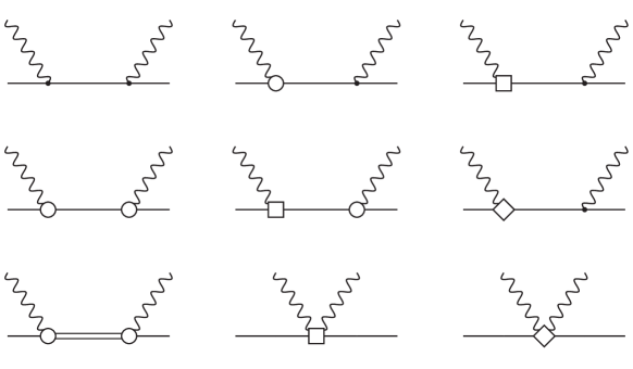
Figure 1: Tree-level diagrams for nucleon Compton scattering which are taken into account in our analysis. Vertices of order $\mathcal{O}(q)$, $\mathcal{O}(q^{2})$, $\mathcal{O}(q^{3})$ and $\mathcal{O}(q^{4})$ are denoted by dots, circles, squares and diamonds, respectively. Solid, wavy and double lines refer to nucleons, photons and $\Delta$-isobars, respectively. Time-reversed and crossed diagrams as well as the diagrams with insertions of the nucleon self-energy contact terms are not shown.

Loop diagrams start to contribute at order $q^{3}$($\epsilon^{3}$). The corresponding sets of diagrams are shown in Fig. 2 for the $q^{3}$-loops and in Fig. 3 for the $\epsilon^{3}$-loops. The subleading $q^{4}$-loop diagrams are shown in Fig. 4.

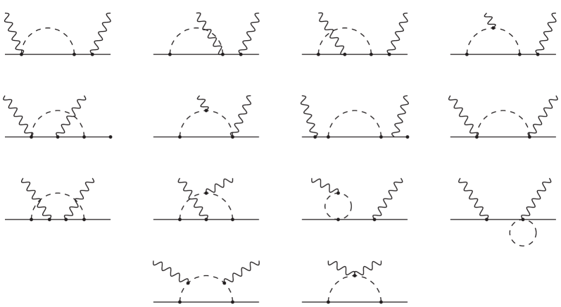
Figure 2: $\mathcal{O}(q^{3})$ loop diagrams for nucleon Compton scattering. Dashed lines refer to pions. All vertices are from the leading order Lagrangians $\mathcal{L}_{\pi\pi}^{(2)}$ and $\mathcal{L}_{\pi N}^{(1)}$. Time-reversed and crossed diagrams are not shown.

Figure 3: $\mathcal{O}(\epsilon^{3})$ loop diagrams for nucleon Compton scattering. All vertices are from the leading order Lagrangians $\mathcal{L}_{\pi\pi}^{(2)}$, $\mathcal{L}_{\pi N}^{(1)}$, $\mathcal{L}^{(1)}_{\pi N\Delta}$ and $\mathcal{L}^{(1)}_{\pi\Delta\Delta}$. Double lines denote the $\Delta$. Time-reversed and crossed diagrams are not shown.

Figure 4: $\mathcal{O}(q^{4})$ loop diagrams for nucleon Compton scattering. Dots denote the leading order vertices and circles denote the vertices from $\mathcal{L}_{\pi N}^{(2)}$. Time-reversed and crossed diagrams are not shown.

II.3 Renormalization

The ultraviolet divergencies appearing in loop integrals are treated by means of dimensional regularization. Divergent parts of the integrals are cancelled by the corresponding counter terms of the Lagrangian, and the resulting amplitude is expressed in terms of the finite quantities such as renormalized low-energy constants, physical masses and coupling constants. Due to the presence of an additional hard scale (the nucleon or $\Delta$ mass), baryonic loops contain power-counting-violating terms Gasser et al. (1988). Since such terms are local, they can be absorbed by a redefinition of the low-energy constants of the effective Lagrangian. In this work, we adopt the extended on-mass-shell renormalization scheme (EOMS) Fuchs et al. (2003) in a combination with on-shell renormalization conditions for the nucleon mass and magnetic moments.

For the nucleon mass and wave-function renormalization, we impose the on-shell conditions

$$\Sigma_{N}(m_{N})=0\ \text{and}\ \Sigma_{N}^{\prime}(m_{N})=0,$$ (10)

with $\Sigma_{N}(\not{p})$ being the nucleon self-energy. By doing so, we fix the bare nucleon mass $m$ and the field normalization factor $Z_{N}$. The explicit formulae relating the physical and bare parameters can be found in Yao et al. (2016). In what follows, we will denote the physical nucleon mass by $m$, which will not lead to a confusion since the bare nucleon mass will not be discussed anymore.

In a complete analogy with the nucleon field, we renormalize the $\Delta$ field. However, at the order we are working there are no loop corrections to the $\Delta$ self-energy. For the calculation of the static nucleon polarizabilites, we us the real Breit-Wigner mass of the $\Delta$. The precise value of the renormalized $\Delta$ mass is irrelevant under the kinematic conditions considered. On the other hand, for calculation of the dynamical nucleon polarizabilites, in order to be able to describe the $\Delta$ region, we implement the complex-mass scheme Denner et al. (1999); Denner and Dittmaier (2006) for the $\Delta$ resonance and use the complex $\Delta$ pole mass taking the resonance width into account explicitly.

For the renormalized constants $\bar{c}_{6}$ and $\bar{c}_{7}$, we use the on-shell condition for the nucleon magnetic moments:

$$\bar{c}_{6}=\kappa_{p}-\kappa_{n}\ \text{ and }\ \bar{c}_{7}=\kappa_{n}\,.$$ (11)

The explicit relation between $\bar{c}_{6}$ and $\bar{c}_{7}$ and the bare constants $c_{6}$ and $c_{7}$ is given in Appendix E.

For the remaining low-energy constants $\xi_{i}$ we employ the EOMS renormalization scheme. The renormalized LECs $\bar{\xi}_{i}$ are related to the bare quantities as follows:

$$\xi_{i}=\bar{\xi}_{i}-\frac{\beta_{\xi_{i}}}{F^{2}}\frac{A_{0}(M^{2})}{2M^{2}}+\frac{\Delta_{\xi_{i}}}{16\pi^{2}F^{2}}\,,$$

$$\xi_{i}\in\{d_{6},d_{7},e_{54},e_{74},e_{89},e_{89},e_{90},e_{91},e_{92},e_{93},e_{94},e_{117},e_{118}\}\,,$$ (12)

with the $\beta$ functions:

$$\beta_{d_{6}}=-\frac{1-g_{A}^{2}}{6}+\frac{40h_{A}}{81}\,,\ \beta_{d_{7}}=\frac{5h_{A}^{2}}{54}\,,$$

$$\beta_{e_{54}}=0\,,\ \beta_{e_{74}}=\frac{1-g_{A}^{2}+4c_{4}}{12m}\,,$$

$$\beta_{e_{91}}=\beta_{e_{92}}=0\,,\ 2\beta_{e_{89}}+\beta_{e_{93}}+\beta_{e_{118}}=\frac{c_{2}}{12}\,,$$

$$2\beta_{e_{90}}+\beta_{e_{94}}+\beta_{e_{117}}=-\frac{c_{2}}{3}\,,$$ (13)

and the finite shifts

$$\Delta_{d_{6}}=-\frac{g_{A}^{2}c_{6}}{8}\,,\ \Delta_{d_{7}}=\frac{3g_{A}^{2}(c_{6}+2c_{7})}{16}\,.$$ (14)

The constants $e_{i}$ do not receive finite shifts due to the power-counting violation because we do not consider loop diagrams of order higher than $\mathcal{O}(q^{4})$. The finite shifts for $d_{6}$ and $d_{7}$ reproduce those obtained in Fuchs et al. (2004) (note a different definition of the LECs). The constants $e_{54}$ and $e_{74}$ do not contribute to the nucleon polarizabilites after subtracting the Born terms. Nevertheless, we provide the corresponding $\beta$ functions for completeness. The LECs $e_{89}$, $e_{90}$, $e_{93}$, $e_{94}$, $e_{117}$, $e_{118}$ enter the nucleon Compton scattering amplitude only in the linear combinations $2e_{89}+e_{93}+e_{118}$ and $2e_{90}+e_{94}+e_{117}$, for which the $\beta$ functions are given in Eq. (13).

The pion tadpole function in $d\approx 4$ dimensions is equal to (see Eq. (39))

$$A_{0}(M)=-2M^{2}\left(\bar{\lambda}+\frac{1}{32\pi^{2}}\ln\left(\frac{M^{2}}{\mu^{2}}\right)\right)\,,$$

$$\bar{\lambda}=\frac{1}{16\pi^{2}}\left(\frac{1}{d-4}+\frac{1}{2}(\gamma_{\text{E}}-\ln(4\pi)-1)\right)\,.$$ (15)

Here, $\gamma_{\text{E}}$ is the Euler-Mascheroni constant and $\mu$ is the renormalization scale. The divergencies remaining after the renormalization of the LECs are treated in the $\widetilde{\mathrm{M}S}$ Fuchs et al. (2003); Gasser and Leutwyler (1984) scheme, i.e. we set $\bar{\lambda}=0$. We have checked that the residual renormalization scale dependence of the amplitude is of a higher order than we are working.

In what follows, we will omit the bars over the renormalized LECs.

III Formalism

We consider nucleon Compton scattering $\gamma N\to\gamma N$ with the momenta of the initial (final) proton and photon denoted as $p$ ($p^{\prime}$) and $q$ ($q^{\prime}$), respectively. We study the cases of real Compton scattering with $q^{2}=q^{\prime 2}=0$ and of double virtual Compton scattering with $Q^{2}=-q^{2}=-q^{\prime 2}$.

In order to calculate the nucleon polarizabilites, we decompose the scattering amplitude $T(q^{2},z,\omega)$ in the Breit frame, where $\omega$ and $z$ are the photon energy and scattering angle, in terms of twelve functions $A_{i}$:

$$T(q^{2},z,\omega)=2m\sum_{i=1}^{12}A_{i}(q^{2},z,\omega)\chi_{i}\,,$$ (16)

with

$$\chi_{1} =\vec{\epsilon}\cdot\vec{\epsilon}^{*}\,,$$

$$\chi_{2} =(\hat{q}\times\vec{\epsilon})\cdot(\hat{q}^{\prime}\times\vec{\epsilon}^{\prime})\,,$$

$$\chi_{3} =\hat{q}\cdot\vec{\epsilon}\;\hat{q}\cdot\vec{\epsilon}^{\prime*}+\hat{q}^{\prime}\cdot\vec{\epsilon}\;\hat{q}^{\prime}\cdot\vec{\epsilon}^{\prime*}\,,$$

$$\chi_{4} =\hat{q}\cdot\vec{\epsilon}\;\hat{q}^{\prime}\cdot\vec{\epsilon}^{\prime*}\,,$$

$$\chi_{5} =i\sigma\cdot\vec{\epsilon}\times\vec{\epsilon}^{\prime*}\,,$$

$$\chi_{6} =i\sigma\cdot(\hat{q}\times\vec{\epsilon})\times(\hat{q}^{\prime}\times\vec{\epsilon}^{\prime})\,,$$

$$\chi_{7} =i(\hat{q}\cdot\vec{\epsilon}\times\vec{\epsilon}^{\prime*}\vec{\sigma}\cdot\hat{q}+\hat{q}^{\prime}\cdot\vec{\epsilon}\times\vec{\epsilon}^{\prime*}\vec{\sigma}\cdot\hat{q}^{\prime})\,,$$

$$\chi_{8} =i(\hat{q}\cdot\vec{\epsilon}\times\vec{\epsilon}^{\prime*}\vec{\sigma}\cdot\hat{q}^{\prime}+\hat{q}^{\prime}\cdot\vec{\epsilon}\times\vec{\epsilon}^{\prime*}\vec{\sigma}\cdot\hat{q})\,,$$

$$\chi_{9} =i\hat{q}\cdot\vec{\epsilon}\;\hat{q}^{\prime}\cdot\vec{\epsilon}^{\prime*}\vec{\sigma}\cdot\hat{q}\times\hat{q}^{\prime}\,,$$

$$\chi_{10} =i(\hat{q}\cdot\vec{\epsilon}\;\hat{q}\cdot\vec{\epsilon}^{\prime*}\vec{\sigma}\cdot\hat{q}\times\hat{q}^{\prime}+\hat{q}^{\prime}\cdot\vec{\epsilon}\;\hat{q}^{\prime}\cdot\vec{\epsilon}^{\prime*}\vec{\sigma}\cdot\hat{q}\times\hat{q}^{\prime})\,,$$

$$\chi_{11} =i(\hat{q}^{\prime}\cdot\vec{\epsilon}^{\prime*}\vec{\sigma}\cdot\vec{\epsilon}\times\hat{q}-\hat{q}\cdot\vec{\epsilon}\;\vec{\sigma}\cdot\vec{\epsilon}^{\prime*}\times\hat{q}^{\prime})\,,$$

$$\chi_{12} =i(\hat{q}^{\prime}\cdot\vec{\epsilon}^{\prime*}\vec{\sigma}\cdot\vec{\epsilon}\times\hat{q}^{\prime}-\hat{q}\cdot\vec{\epsilon}\;\vec{\sigma}\cdot\vec{\epsilon}^{\prime*}\times\hat{q})\,.$$ (17)

The initial (final) photon polarization vector $\epsilon_{\mu}$ ($\epsilon^{\prime}_{\mu}$) is defined in the Coulomb gauge ($\epsilon_{0}=\epsilon^{\prime}_{0}=0$). The amplitude (16) is supposed to be sandwiched between the Pauli spinors of the initial and final nucleon.

Given the presence of the Pauli matrices $\vec{\sigma}$ in Eq. (17), one can see that there are four spin-independent structures $\chi_{1}-\chi_{4}$ and eight spin-dependent structures $\chi_{5}-\chi_{12}$. All $\chi_{i}$ obey crossing-invariance. For real Compton scattering, only $\chi_{1}$, $\chi_{2}$, $\chi_{5}$, $\chi_{6}$, $\chi_{7}$, $\chi_{8}$ survive.

The Born terms have to be subtracted from the amplitude as explained, e.g., in Lensky et al. (2018) in order to exclude the contributions with unexcited nucleons in the intermediate state. This procedure essentially reduces to subtracting the tree-level $Q^{2}=0$ nucleon-pole diagrams with the nucleon charge and magnetic moments replaced by the full Dirac and Pauli form factors calculated consistently within our scheme applying the same power counting. The anomalous pion $t$-channel exchange diagram is also excluded from the definition of the polarizabilites.

The amplitudes $A_{i}$ can be expressed in terms of the nucleon polarizabilites by performing an expansion in $\omega$ around $\omega=0$:

$$A_{1}(\omega) =\frac{4\pi E_{N}}{m}\bigg{[}\alpha_{\text{E1}}\omega^{2}+\frac{\omega^{4}}{12}(2z\alpha_{\text{E2}}-\beta_{\text{M2}}+12\alpha_{\text{E1}\nu})+\frac{\omega^{6}}{2700}\left((30z^{2}-2)\alpha_{\text{E3}}-20z\beta_{\text{M3}}\right.$$

$$\hskip 28.45274pt+\left.450z\alpha_{\text{E2}\nu}-225\beta_{\text{M2}\nu}+2700\alpha_{\text{E1}\nu^{2}}\right)+\mathcal{O}(\omega^{8})\bigg{]}\,,$$

$$A_{2}(\omega) =\frac{4\pi E_{N}}{m}\bigg{[}\beta_{\text{M1}}\omega^{2}+\frac{\omega^{4}}{12}(2z\beta_{\text{M2}}-\alpha_{\text{E2}}+12\beta_{\text{M1}\nu})+\frac{\omega^{6}}{2700}\left((30z^{2}-2)\beta_{\text{M3}}-20z\alpha_{\text{E3}}\right.$$

$$\hskip 28.45274pt+\left.450z\beta_{\text{M2}\nu}-225\alpha_{\text{E2}\nu}+2700\beta_{\text{M1}\nu^{2}}\right)+\mathcal{O}(\omega^{8})\bigg{]}\,,$$

$$A_{5}(\omega) =\frac{4\pi E_{N}}{m}\bigg{[}(\gamma_{\text{E1E1}}-\gamma_{\text{E1M2}})\omega^{3}+\frac{\omega^{5}}{5}\left(20z\gamma_{\text{E2E2}}+5\gamma_{\text{E1E1}\nu}-10z\gamma_{\text{E2M3}}\right.$$

$$\hskip 28.45274pt-\left.5\gamma_{\text{E1M2}\nu}+2\gamma_{\text{M2E3}}+5\gamma_{\text{M2M2}}\right)+\mathcal{O}(\omega^{7})\bigg{]}\,,$$

$$A_{6}(\omega) =\frac{4\pi E_{N}}{m}\bigg{[}(\gamma_{\text{M1M1}}-\gamma_{\text{M1E2}})\omega^{3}+\frac{\omega^{5}}{5}\left(20z\gamma_{\text{M2M2}}+5\gamma_{\text{M1M1}\nu}-10z\gamma_{\text{M2E3}}\right.$$

$$\hskip 28.45274pt-\left.5\gamma_{\text{M1E2}\nu}+2\gamma_{\text{E2M3}}+5\gamma_{\text{E2E2}}\right)+\mathcal{O}(\omega^{7})\bigg{]}\,,$$

$$A_{7}(\omega) =\frac{4\pi E_{N}}{m}\bigg{[}\gamma_{\text{E1M2}}\omega^{3}+\frac{\omega^{5}}{5}\left(15z\gamma_{\text{E2M3}}+5\gamma_{\text{E1M2}\nu}-7\gamma_{\text{M2E3}}-\!10\gamma_{\text{M2M2}}\right)+\mathcal{O}(\omega^{7})\bigg{]}\,,$$

$$A_{8}(\omega) =\frac{4\pi E_{N}}{m}\bigg{[}\gamma_{\text{M1E2}}\omega^{3}+\frac{\omega^{5}}{5}\left(15z\gamma_{\text{M2E3}}+5\gamma_{\text{M1E2}\nu}-7\gamma_{\text{E2M3}}-10\gamma_{\text{E2E2}}\right)+\mathcal{O}(\omega^{7})\bigg{]}\,,$$ (18)

where $E_{N}$ is the nucleon energy. We also introduce the linear combinations corresponding to the forward and backward spin polarizabilites $\gamma_{0}$ and $\gamma_{\pi}$

$$\gamma_{0} =-\gamma_{\text{E1E1}}-\gamma_{\text{M1M1}}-\gamma_{\text{E1M2}}-\gamma_{\text{M1E2}}\,,$$

$$\gamma_{\pi} =-\gamma_{\text{E1E1}}+\gamma_{\text{M1M1}}-\gamma_{\text{E1M2}}+\gamma_{\text{M1E2}}\,,$$ (19)

the higher-order forward spin polarizabilty

$$\bar{\gamma}_{0} =-\gamma_{\text{E1E1}\nu}-\gamma_{\text{M1M1}\nu}-\gamma_{\text{M1E2}\nu}-\gamma_{\text{E1M2}\nu}$$

$$\phantom{=}-\gamma_{\text{E2E2}}-\gamma_{\text{M2M2}}-\tfrac{8}{5}(\gamma_{\text{E2M3}}+\gamma_{\text{M2E3}})\,,$$ (20)

as well as the longitudinal-transverse spin polarizability

$$\delta_{\text{LT}} =-\frac{1}{6}\frac{d^{3}}{d\omega^{3}}\bigg{\{}\frac{m}{4\pi E_{N}}\Big{[}A_{5}(\omega)+A_{11}(\omega)+A_{12}(\omega)\Big{]}\bigg{\}}\bigg{\arrowvert}_{\omega=0}\,.$$ (21)

There are similar but different amplitude decompositions used in the literature, which leads to different relations of those amplitudes to the nucleon polarizabilites. For ease of comparison, we provide the transformation matrix from the vector of amplitudes $A_{\text{this work}}=(A_{1},A_{2},A_{5},A_{6},A_{7},A_{8})$ defined in Eq. (17) to the vector of amplitudes $A_{\text{LMP}}=(A_{1},A_{2},A_{3},A_{4},A_{5},A_{6})$ considered in Lensky et al. (2015)

$$A_{\text{LMP}}=LA_{\text{this work}}\,,\ L=\left(\begin{array}[]{cccccc}1&z&0&0&0&0\\ 0&-1&0&0&0&0\\ 0&0&1&z&2&2z\\ 0&0&0&1&0&0\\ 0&0&0&-1&0&-1\\ 0&0&0&0&-1&0\end{array}\right)\,.$$ (28)

In this work, we also analyze the so-called dynamical polarizabilites defined in terms of the center-of-mass multipoles as follows (see, e.g., Griesshammer and Hemmert (2002); Hildebrandt et al. (2004); Lensky et al. (2015); Guiasu and Radescu (1979)):

$$\alpha_{\text{E}l}(\omega)=l^{2}(2l-1)!!\frac{(l+1)f_{EE}^{l+}+lf_{EE}^{l-}}{\omega^{2l}}\,,\ \beta_{\text{M}l}(\omega)=l^{2}(2l-1)!!\frac{(l+1)f_{MM}^{l+}+lf_{MM}^{l-}}{\omega^{2l}}\,,$$

$$\gamma_{\text{E}l\text{E}l}(\omega)=\frac{f_{EE}^{l+}-f_{EE}^{l-}}{\omega^{2l+1}}\,,\ \gamma_{\text{E}l\text{M}l\pm 1}(\omega)=(2l\pm 1)!\frac{f_{EM}^{l\pm}}{\omega^{2l\pm 1}}\,,$$

$$\gamma_{\text{M}l\text{M}l}(\omega)=\frac{f_{MM}^{l+}-f_{MM}^{l-}}{\omega^{2l+1}}\,,\ \gamma_{\text{M}l\text{E}l\pm 1}(\omega)=(2l\pm 1)!\frac{f_{ME}^{l\pm}}{\omega^{2l\pm 1}}\,,$$ (29)

for $l=1,2$. Note that in contrast to the equations above, in Eq. (29), $\omega$ denotes the center-of-mass photon energy.

IV Results

We are now in the position to present our numerical results for various proton and neutron polarizabilities calculated up to order $\mathcal{O}(\epsilon^{3}+q^{4})$. Specifically, we consider the following polarizabilities: spin-independent (scalar) dipole, quadrupole, octupole, dispersive dipole and quadrupole polarizabilities as well as dipole, quadrupole and dispersive dipole spin polarizabilities. We also discuss selected generalized (i.e. $Q^{2}$-dependent) and dynamical (i.e. energy-dependent) polarizabilities.

As already mentioned above, most of the results we present are pure predictions and contain no free parameters. The only exceptions are the spin-independent dipole polarizabilities $\alpha_{\text{E1}}$ and $\beta_{\text{M1}}$ at order $\mathcal{O}(q^{4})$ or $\mathcal{O}(\epsilon^{3}+q^{4})$, which are fitted to the experimental values. All remaining parameters are taken from other processes and are collected in Tables 1, 2 and 3.

$\alpha_{EM}^{-1}$	$M$ [MeV]	$F_{\pi}$ [MeV]	$m$ [MeV]	$m_{\Delta}$ [MeV]	$g_{A}$	$c_{6}$	$c_{7}$	$h_{A}$	$b_{1}\;[m^{-1}]$
$137.036$	$138.04$	$92.21$	$938.9$	$1232$	$1.27$	$3.706$	$-1.913$	$1.43$	$-4.98$

Table 1: Parameters used in the current work. The values of $\alpha_{EM}$, $M$, $m$, $m_{\Delta}$, $g_{A}$, $F_{\pi}$ are taken from Tanabashi et al. (2018). The LECs $c_{6}$ and $c_{7}$ are related to the proton and neutron magnetic moment and $d_{6}$ and $d_{6}$ with the proton and neutron charge radii Fuchs et al. (2004). The values of the LECs $b_{1}$ and $h_{A}$ are extracted from the electromagnetic and strong width of the $\Delta$-resonance, respectively, see Bernard et al. (2013) for details and explicit expressions. For the static polarizabilities we use the real $\Delta$ mass as given in the Table, whereas for the generalized polarizabilities we use the pole mass $m_{\Delta}=(1210-50i)\text{ MeV}$.

	$\phantom{-}q^{3}$	$\phantom{-}q^{4}$	$\phantom{-}\epsilon^{3}$	$\phantom{-}q^{4}+\epsilon^{3}$
$c_{1}\;[m^{-1}]$	$-0.94\pm 0.02$	$-1.05\pm 0.03$	$-1.05\pm 0.03$	$-1.05\pm 0.03$
$c_{2}\;[m^{-1}]$	$\phantom{-}2.39\pm 0.03$	$\phantom{-}3.15\pm 0.03$	$\phantom{-}0.96\pm 0.11$	$\phantom{-}0.96\pm 0.11$
$c_{3}\;[m^{-1}]$	$-4.60\pm 0.05$	$-5.35\pm 0.06$	$-2.13\pm 0.19$	$-2.13\pm 0.19$

Table 2: Numerical values of the low energy constants used in the current work as determined by matching the solution of Roy-Steiner equations for $\pi N$ scattering Ditsche et al. (2012) to chiral perturbation theory in Siemens et al. (2017). The values for $q^{4}+\epsilon^{3}$ correspond to the $\epsilon^{3}$ calculation of Siemens et al. (2017).

	$\phantom{-}q^{3}$	$\phantom{-}q^{4}$	$\phantom{-}\epsilon^{3}$	$\phantom{-}q^{4}+\epsilon^{3}$
$d_{6}\;[m^{-2}]$	$-0.61$ Fuchs et al. (2004)	$-0.61$ Fuchs et al. (2004)	$-0.80\pm 0.04$	$-1.27\pm 0.05$
$d_{7}\;[m^{-2}]$	$-0.43$ Fuchs et al. (2004)	$-0.44$ Fuchs et al. (2004)	$-0.44\pm 0.01$	$-0.46\pm 0.01$
$e_{91}\;[m^{-3}]$	$\ldots$	$-0.04\pm 0.22$	$\ldots$	$-0.46\pm 0.23$
$e_{92}\;[m^{-3}]$	$\ldots$	$-0.29\pm 0.79$	$\ldots$	$-0.22\pm 0.80$
$(2e_{89}+e_{93}+e_{118})\;[m^{-3}]$	$\ldots$	$-0.07\pm 0.23$	$\ldots$	$-2.53\pm 0.50$
$(2e_{90}+e_{94}+e_{117})\;[m^{-3}]$	$\ldots$	$-1.76\pm 0.80$	$\ldots$	$\phantom{-}2.02\pm 1.20$

Table 3: Numerical values of the low-energy constants obtained from the fit to the empirical values of the electric radius of the proton and neutron ($d_{i}$) and the proton and neutron spin-independent polarizabilites ($e_{i}$). Note that the $e_{i}$ enter at fourth order and therefore do not have values for $q^{3}$ and $\epsilon^{3}$.

In the course of the calculation we have used our own code written in $Mathematica$ Wolfram Research, Inc. and FORM Kuipers et al. (2013) for the analytical calculation of Feynman diagrams. The numerical evaluation of loop integrals have been performed with help of the Mathematica package Package-X Patel (2017). We have also used our own Fortran code for estimating the theoretical errors.

For our complete results at order $\mathcal{O}(\epsilon^{3}+q^{4})$, we also provide estimations of the theoretical errors originating from two sources, namely the uncertainties in the input parameters and the errors caused by the truncation of the small-scale expansion. For the latter uncertainty, we adopt the Bayesian model used in Epelbaum et al. (2019a, b) based on the ideas developed in Furnstahl et al. (2015); Melendez et al. (2017, 2019), see Rijneveen et al. (2020) for a recent application to radiative pion photoproduction. The observables are assumed to be expanded in parameter $Q$ given by

$$Q={\rm max}\bigg{(}\frac{M^{\rm eff}}{\Lambda_{\rm b}},\;\frac{\sqrt{Q^{2}}}{\Lambda_{\rm b}},\;\frac{\omega}{\Lambda_{\rm b}}\bigg{)}\,,$$ (30)

where $Q^{2}$ on the right-hand side is the virtuality of the photon, and $\omega$ is the photon energy in the case of dynamical polarizabilities. The soft and hard scales are chosen to be $M^{\rm eff}=200$ MeV and $\Lambda_{\rm b}=700$ MeV in accordance with Epelbaum (2019). Following Epelbaum et al. (2019a, b), we utilize the Gaussian prior distribution for the expansion coefficients $c_{i}$:

$${\rm pr}(c_{i}|\bar{c})=\frac{1}{\sqrt{2\pi}\bar{c}}\,e^{-c_{i}^{2}/(2\bar{c}^{2})},\quad\quad{\rm pr}(\bar{c})=\frac{1}{\ln(\bar{c}_{>}/\bar{c}_{<})}\,\frac{1}{\bar{c}}\,\theta(\bar{c}-\bar{c}_{<})\,\theta(\bar{c}_{>}-\bar{c})\,,$$ (31)

with the cut offs $\bar{c}_{<}=0.5$ and $\bar{c}_{>}=10$. Further details on the employed Bayesian model can be found in Epelbaum et al. (2019a, b).

In the following sections, we provide a detailed comparison of our results with the available experimental/empirical data as well as with other theoretical approaches based on chiral perturbation theory and on fixed-$t$ dispersion relations. We also discuss generalized polarizabilities, investigate the convergence pattern of the $1/m$-expansion for the calculated polarizabilities and compare the results of covariant $\chi$PT with the heavy baryon approach. Last but not least, we emphasize that the resulting large absolute numerical values of the octupole polarizabilites are merely due to the numerical factors in their definition, which makes them consistent with the definition of the polarizabilites for composite systems.

IV.1 Scalar dipole polarizabilites

We start by considering the spin-independent dipole nucleon polarizabilites $\alpha_{\text{E1}}$ and $\beta_{\text{M1}}$. The results of the calculations at order $\mathcal{O}(q^{4})$ and $\mathcal{O}(\epsilon^{3}+q^{4})$ as well as the individual contributions from orders $\mathcal{O}(q^{3})$, $\mathcal{O}(q^{4})$ pion-nucleon loops, $\mathcal{O}(\epsilon^{3})$ $\pi\Delta$-loops and tree-level $\Delta$-pole graphs are presented in Table 4.

	Proton		Neutron
	$\phantom{-}\phantom{1}\alpha_{\text{E1}}$	$\phantom{-}\phantom{1}\beta_{\text{M1}}$	$\phantom{-}\phantom{1}\alpha_{\text{E1}}$	$\phantom{-}\phantom{1}\beta_{\text{M1}}$
$q^{3}$ (without $\Delta$)	$\phantom{-}\phantom{1}7.04$	$\phantom{1}{-1.85}$	$\phantom{-}\phantom{1}9.51$	$\phantom{1}{-1.10}$
$q^{4}$ (without $\Delta$)	$\phantom{-}\phantom{1}4.16$	$\phantom{-}\phantom{1}4.35$	$\phantom{-}\phantom{1}2.09$	$\phantom{-}\phantom{1}4.80$
Total (without $\Delta$)	$\phantom{-}11.20$	$\phantom{-}\phantom{1}2.50$	$\phantom{-}11.60$	$\phantom{-}\phantom{1}3.70$
$q^{3}$	$\phantom{-}\phantom{1}7.04$	$\phantom{1}{-1.85}$	$\phantom{-}\phantom{1}9.51$	$\phantom{1}{-1.10}$
$\epsilon^{3}$ $\pi\Delta$ loop	$\phantom{1}{-1.45}$	$\phantom{-}\phantom{1}5.54$	$\phantom{-}\phantom{1}2.78$	$\phantom{-}\phantom{1}0.96$
$\epsilon^{3}$ $\Delta$ tree	$\phantom{1}{-3.78}$	$\phantom{-}11.96$	$\phantom{1}{-3.78}$	$\phantom{-}11.96$
$q^{4}$	$\phantom{-}\phantom{1}9.40$	$-13.16$	$\phantom{-}\phantom{1}3.10$	$\phantom{1}{-8.12}$
Total	$\phantom{1}11.20$	$\phantom{1}\phantom{1}2.50$	$\phantom{1}11.60$	$\phantom{1}\phantom{1}3.70$
$\mathcal{O}(p^{3})$ $\pi$N loops Lensky et al. (2015)	$\phantom{-}\phantom{1}6.8$	$\phantom{1}{-1.8}$	$\phantom{-}\phantom{1}9.4$	$\phantom{1}{-1.1}$
$\mathcal{O}(p^{7/2})$ $\pi\Delta$ loops Lensky et al. (2015)	$\phantom{-}\phantom{1}4.4$	$\phantom{1}{-1.4}$	$\phantom{-}\phantom{1}4.4$	$\phantom{1}{-1.4}$
$\Delta$ pole Lensky et al. (2015)	$\phantom{1}{-0.1}$	$\phantom{-}\phantom{1}7.1$	$\phantom{1}{-0.1}$	$\phantom{-}\phantom{1}7.1$
Total Lensky et al. (2015)	$\phantom{-}11.2\pm 0.7$	$\phantom{-}\phantom{1}3.9\pm 0.7$	$\phantom{-}13.7\pm 3.1$	$\phantom{-}\phantom{1}4.6\pm 2.7$
Fixed-$t$ DR Babusci et al. (1998); Olmos de Leon et al. (2001)	$\phantom{-}12.1$	$\phantom{-}\phantom{1}1.6$	$\phantom{-}12.5$	$\phantom{-}\phantom{1}2.7$
HB$\chi$PT fit McGovern et al. (2013)	$\phantom{-}10.65\pm 0.50$	$\phantom{-}\phantom{1}3.15\pm 0.50$	$\phantom{-}11.55\pm 1.5$	$\phantom{-}\phantom{1}3.65\pm 1.5$
B$\chi$PT fit Lensky and McGovern (2014)	$\phantom{-}10.6\pm 0.5$	$\phantom{-}\phantom{1}3.2\pm 0.5$	$\phantom{-}\ldots$	$\phantom{-}\phantom{1}\ldots$
PDG Tanabashi et al. (2018)	$\phantom{-}11.2\pm 0.4$	$\phantom{-}\phantom{1}2.5\pm 0.4$	$\phantom{-}11.6\pm 1.5$	$\phantom{-}\phantom{1}3.7\pm 2.0$

Table 4: Numerical values for the spin-independent dipole polarizabilities of the proton and the neutron in $10^{-4}\text{fm}^{3}$. The values are compared with the results calculated within the $\delta$-counting scheme and obtained using fixed-$t$ dispersion relations.

At order $\mathcal{O}(q^{4})$, there appear low energy constants in the effective Lagrangian that contribute to the nucleon Compton scattering. We adjust four relevant linear combinations of them ($e_{91}$, $e_{92}$, $2e_{89}+e_{93}+e_{118}$ and $2e_{90}+e_{94}+e_{117}$) in such a way as to reproduce the empirical values of the proton and neutron spin-independent dipole polarizabilities, see Table 3.

In the case of the $\Delta$-less theory, the contribution at order $\mathcal{O}(q^{4})$ for the electric polarizability $\alpha_{\text{E1}}$ of the proton (neutron) is about two (five) times smaller than the one at order $\mathcal{O}(q^{3})$, which is an indication of a reasonable convergence of the chiral expansion. For the magnetic polarizabilities $\beta_{\text{M1}}$, due to some cancellations among $\mathcal{O}(q^{3})$ loops, the contributions at order $\mathcal{O}(q^{4})$ are larger than the ones at order $\mathcal{O}(q^{3})$ but are, nevertheless, comparable with those for the $\alpha_{\text{E1}}$.

In the $\Delta$-full scheme, the $\mathcal{O}(q^{4})$ terms (that differ from the ones in the $\Delta$-less case by the values of $c_{i}$’s and $e_{i}$’s) are significantly larger. This feature can be traced back to the sizable $\mathcal{O}(\epsilon^{3})$ contributions, especially from the $\Delta$-pole tree-level diagrams, that need to be compensated by adjusting the relevant contact terms. Such contributions appear to be demoted to higher orders in the $\Delta$-less scheme. Their importance for other polarizabilites will, however, be demonstrated below. Thus, a seemingly better convergence of the $\Delta$-less approach for the dipole polarizabilites can be argued to be accidental. Notice further that the convergence issues are not really relevant for the dipole spin-independent polarizabilites at the order we are working due to the presence of the corresponding compensating contact terms in the Lagrangian.

In Table 4, we also provide for comparison the values for the dipole spin-independent polarizabilites obtained by analyzing experimental data using fixed-$t$ dispersion relations Babusci et al. (1998); Olmos de Leon et al. (2001), and by fitting experimental data employing various versions of the $\delta$-counting schemes (with the loop diagrams calculated utilizing the covariant Lensky and McGovern (2014) or heavy-baryon approach McGovern et al. (2013)). It is particularly instructive to compare our results with Lensky et al. (2015), where the individual contributions calculated within the $\delta$-counting scheme are presented. Such a comparison allows one to analyze the importance of the explicit $\Delta$ degrees of freedom and the sensitivity of the results to employed counting schemes for the $\Delta$-nucleon mass difference. There are two main sources of differences between our approach and the one used in Lensky et al. (2015) (apart from slightly different numerical values of the coupling constants). First, different terms in the effective Lagrangian corresponding to the $\gamma N\Delta$ vertex are used. The $\gamma N\Delta$ Lagrangian of Lensky et al. (2015) contains two terms with the so-called magnetic and electric $\gamma N\Delta$-couplings $g_{M}$ and $g_{E}$:

$$\mathcal{L}_{\gamma N\Delta}=\frac{3e}{2m(m_{\Delta}+m)}\bar{N}T_{3}^{\dagger}(ig_{M}\tilde{F}^{\mu\nu}-g_{E}\gamma_{5}F^{\mu\nu})\partial_{\mu}\Delta_{\nu}+h.c.\,,$$ (32)

which in our scheme correspond to the $b_{1}$- and $h_{1}$-terms (the contribution from the $h_{1}$-term is of a higher order in our power counting and does not appear in the current calculations). The two prescriptions are identical when both the nucleon and the Delta are on the mass shell. Otherwise, the difference is compensated by local contact terms of a higher order in the $1/m$-expansion, see Tang and Ellis (1996); Pascalutsa (2001); Krebs et al. (2010, 2009) for a related discussion. Such off-shell effects manifest themselves, e.g., in the tree-level $\Delta$-contribution to the magnetic polarizability $\beta_{\text{M1}}$. Although the residue of the $\Delta$ pole in the magnetic channel is the same in both schemes (the constants $b_{1}$ and $g_{M}$ are roughly in agreement with each other when calculating the magnetic $\gamma N\Delta$ transition form factor), the full result differs almost by a factor of two due to the presence of the non-pole (background) terms. The non-vanishing (and sizable) contribution of the $\Delta$-tree-level diagrams to the electric polarizabilites $\alpha_{\text{E1}}$ is in our scheme a pure $1/m$-effect caused by the induced electric $\gamma N\Delta$ coupling stemming from the particular form of the effective Lagrangian. On the other hand, the $\Delta$ tree-level contribution to $\alpha_{\text{E1}}$ is negligible in the $\delta$-counting scheme because of the smallness of the electric $\gamma N\Delta$ coupling $g_{E}$. Note that terms proportional to $g_{E}^{2}$ ($h_{1}^{2}$) start to contribute only at order $\epsilon^{5}$ in the small-scale-expansion scheme. The observed dependence of the considered polarizabilites on the off-shell effects might be an indication of the importance of such higher order contributions. Fortunately, such $1/m$ effects are strongly suppressed for higher-order polarizabilites as will be shown below.

The second difference between the two schemes is related to power-counting of various diagrams with internal $\Delta$-lines. While the $\pi N$ loops in Lensky et al. (2015) at order $\mathcal{O}(p^{3})$ are identical with the ones included in our $\mathcal{O}(q^{3})$ results, the diagrams with two and three $\Delta$-lines inside the loop are suppressed in the $\delta$-counting and are not included in their leading-order $\pi\Delta$-loop amplitude. On the other hand, such diagrams are required by gauge invariance (notice, however, that in the Coulomb gauge, their contribution is suppressed by a factor $1/m$). In any case, we observe a significant difference between the size of the $\epsilon^{3}$ $\pi\Delta$-loop contributions in our scheme and the $\mathcal{O}(p^{7/2})$ ones of Lensky et al. (2015) involving only the $\pi\Delta$-loops with a single $\Delta$-line.

IV.2 Dipole spin polarizabilites

Next, we consider the dipole spin polarizabilites $\phantom{-}\gamma_{\text{E1E1}}$, $\phantom{-}\gamma_{\text{M1M1}}$, $\phantom{-}\gamma_{\text{E1M2}}$ and $\phantom{-}\gamma_{\text{M1E2}}$. These quantities are less sensitive to the short range dynamics as the relevant contact terms appear at order $\mathcal{O}(q^{5})$. Therefore, one expects a better convergence pattern for them. At the order we are working, the spin polarizabilites are predictions and do not depend on any free parameters. The numerical values of the spin polarizabilites for the proton and neutron are collected in Table 5.

	$\phantom{-}\gamma_{\text{E1E1}}^{(p)}$	$\phantom{-}\gamma_{\text{M1M1}}^{(p)}$	$\phantom{-}\gamma_{\text{E1M2}}^{(p)}$	$\phantom{-}\gamma_{\text{M1E2}}^{(p)}$
$q^{3}$ (without $\Delta$)	$-3.46$	$-0.13$	$\phantom{-}0.57$	$\phantom{-}0.95$
$q^{4}$ (without $\Delta$)	$-0.01$	$\phantom{-}0.49$	$-0.25$	$\phantom{-}0.56$
Total (without $\Delta$)	$-3.47$	$\phantom{-}0.36$	$\phantom{-}0.32$	$\phantom{-}1.51$
$q^{3}$	$-3.46$	$-0.13$	$\phantom{-}0.57$	$\phantom{-}0.95$
$\epsilon^{3}$ $\pi\Delta$ loops	$-0.11$	$\phantom{-}0.58$	$\phantom{-}0.48$	$-0.79$
$\epsilon^{3}$ $\Delta$ tree	$-1.07$	$\phantom{-}3.85$	$-0.88$	$\phantom{-}1.74$
$q^{4}$	$-0.01$	$\phantom{-}0.49$	$-0.25$	$\phantom{-}0.56$
Total	$-4.65\,\begin{subarray}{c}\pm 0.12\\ \pm 0.44\end{subarray}$	$4.80\,\begin{subarray}{c}\pm 0.43\\ \pm 0.44\end{subarray}$	$-0.08\,\begin{subarray}{c}\pm 0.11\\ \pm 0.08\end{subarray}$	$2.47\,\begin{subarray}{c}\pm 0.21\\ \pm 0.26\end{subarray}$
$\mathcal{O}(p^{3})$ $\pi$N loops Lensky et al. (2015)	$-3.4$	$-0.1$	$\phantom{-}0.5$	$\phantom{-}0.9$
$\mathcal{O}(p^{7/2})$ $\pi\Delta$ loops Lensky et al. (2015)	$\phantom{-}0.4$	$-0.2$	$\phantom{-}0.1$	$-0.2$
$\Delta$ pole Lensky et al. (2015)	$-0.4$	$\phantom{-}3.3$	$-0.4$	$\phantom{-}0.4$
Total Lensky et al. (2015)	$-3.3\pm 0.8$	$\phantom{-}2.9\pm 1.5$	$\phantom{-}0.2\pm 0.2$	$\phantom{-}1.1\pm 0.3$
Fixed-$t$ DR Babusci et al. (1998)	$-3.4$	$\phantom{-}2.7$	$\phantom{-}0.3$	$\phantom{-}1.9$
Fixed-$t$ DR Holstein et al. (2000); Hildebrandt et al. (2004); Pasquini et al. (2007)	$-4.3$	$\phantom{-}2.9$	$-0.02$	$\phantom{-}2.2$
HB$\chi$PT fit McGovern et al. (2013); Griesshammer et al. (2016)	$-1.1\pm 1.9$	$\phantom{-}2.2\pm 0.8$	$-0.4\pm 0.6$	$\phantom{-}1.9\pm 0.5$
MAMI 2015 Martel et al. (2015)	$-3.5\pm 1.2$	$\phantom{-}3.16\pm 0.85$	$-0.7\pm 1.2$	$\phantom{-}1.99\pm 0.29$
MAMI 2018 Paudyal et al. (2019)	$-3.18\pm 0.52$	$\phantom{-}2.98\pm 0.43$	$-0.44\pm 0.67$	$\phantom{-}1.58\pm 0.43$
	$\phantom{-}\gamma_{\text{E1E1}}^{(n)}$	$\phantom{-}\gamma_{\text{M1M1}}^{(n)}$	$\phantom{-}\gamma_{\text{E1M2}}^{(n)}$	$\phantom{-}\gamma_{\text{M1E2}}^{(n)}$
$q^{3}$ (without $\Delta$)	$-4.86$	$-0.17$	$\phantom{-}0.61$	$\phantom{-}1.36$
$q^{4}$ (without $\Delta$)	$-0.46$	$\phantom{-}1.42$	$-0.59$	$\phantom{-}0.76$
Total (without $\Delta$)	$-5.32$	$\phantom{-}1.25$	$-0.02$	$\phantom{-}2.12$
$q^{3}$	$-4.86$	$-0.17$	$\phantom{-}0.61$	$\phantom{-}1.36$
$\epsilon^{3}$ $\pi\Delta$ loops	$\phantom{-}0.22$	$\phantom{-}0.12$	$\phantom{-}0.11$	$-0.27$
$\epsilon^{3}$ $\Delta$ tree	$-1.07$	$\phantom{-}3.85$	$-0.88$	$\phantom{-}1.74$
$q^{4}$	$-0.46$	$\phantom{-}1.42$	$-0.59$	$\phantom{-}0.76$
Total	$-6.17\,\begin{subarray}{c}\pm 0.12\\ \pm 0.56\end{subarray}$	$5.22\,\begin{subarray}{c}\pm 0.42\\ \pm 0.59\end{subarray}$	$-0.75\,\begin{subarray}{c}\pm 0.10\\ \pm 0.20\end{subarray}$	$3.59\,\begin{subarray}{c}\pm 0.20\\ \pm 0.37\end{subarray}$
$\mathcal{O}(p^{3})$ $\pi$N loops Lensky et al. (2015)	$-4.7$	$-0.2$	$\phantom{-}0.6$	$\phantom{-}1.3$
$\mathcal{O}(p^{7/2})$ $\pi\Delta$ loops Lensky et al. (2015)	$\phantom{-}0.4$	$-0.2$	$\phantom{-}0.1$	$-0.2$
$\Delta$ pole Lensky et al. (2015)	$-0.4$	$\phantom{-}3.3$	$-0.4$	$\phantom{-}0.4$
Total Lensky et al. (2015)	$-4.7\pm 1.1$	$\phantom{-}2.9\pm 1.5$	$\phantom{-}0.2\pm 0.2$	$\phantom{-}1.6\pm 0.4$
Fixed-$t$ DR Babusci et al. (1998)	$-5.6$	$\phantom{-}3.8$	$-0.7$	$\phantom{-}2.9$
Fixed-$t$ DR Drechsel et al. (2003); Hildebrandt et al. (2004); Lensky et al. (2015)	$-5.9$	$\phantom{-}3.8$	$-0.9$	$\phantom{-}3.1$
HB$\chi$PT fit McGovern et al. (2013); Griesshammer et al. (2016)	$-4.0\pm 1.9$	$\phantom{-}1.3\pm 0.8$	$-0.1\pm 0.6$	$\phantom{-}2.4\pm 0.5$

Table 5: Numerical values for the dipole spin polarizabilities of the proton (upper table) and the neutron (lower table) in $10^{-4}\text{fm}^{4}$. The upper errors originate from the uncertainty in the input parameters, the lower errors come from the truncation of the small-scale expansion. The values are compared with the results calculated within the $\delta$-counting scheme and obtained using fixed-$t$ dispersion relations.

We also provide theoretical errors for our complete scheme at order $\mathcal{O}(q^{4}+\epsilon^{3})$. The upper error reflects the uncertainty in the input parameters, whereas the lower value is the Bayesian estimate of the error coming from the truncation of the small-scale expansion.

The experimental values in Table 5 are obtained from the dispersion-relation analysis of the double-polarized Compton scattering asymmetries $\Sigma_{3}$ and $\Sigma_{2x}$ Martel et al. (2015), and, in a newer experiment, also $\Sigma_{2z}$ Paudyal et al. (2019).

Our predictions for the proton spin polarizabilites at order $\mathcal{O}(q^{4}+\epsilon^{3})$ agree with the experimental values of Martel et al. (2015) within the errors with only a slight deviation for $\gamma_{\text{M1M1}}$. The deviation from the values extracted in the recent MAMI experiment Paudyal et al. (2019) are somewhat larger. Note that the $\Delta$-less approach fails to reproduce $\gamma_{\text{M1M1}}$ for the proton because of the missing $\Delta$-pole contribution, which would appear as a contact term at order $\mathcal{O}(q^{5})$.

The contributions of order $\mathcal{O}(q^{4})$ are in all cases significantly smaller than the leading terms of order $\mathcal{O}(q^{3}+\epsilon^{3})$ in the $\Delta$-full scheme (except for $\gamma_{\text{E1M2}}$ where the leading-order result is small due to cancellations between individual contributions), which is an indication of a reasonable convergence of the small-scale expansion. The smallness of the $\mathcal{O}(q^{4})$-terms can probably also be traced back to the fact that the diagrams containing $c_{1}$, $c_{2}$ and $c_{3}$ vertices do not contribute to spin polarizabilites. Our $\Delta$-full results also agree well with the values obtained from the fixed-$t$ dispersion relations for the proton and the neutron, except for $\gamma_{\text{M1M1}}$, where our prediction appears to be somewhat larger.

In Table 6, we present the results for the forward and backward spin polarizabilites $\gamma_{0}$ and $\gamma_{\pi}$ which are the linear combinations of the four spin polarizabilites and can be more easily accessed experimentally. For these quantities, the agreement with the experimental values is slightly worse, as can be seen from Table  6.

	$\phantom{-}\gamma_{0}^{(p)}$	$\phantom{-}\gamma_{\pi}^{(p)}$	$\phantom{-}\bar{\gamma}_{0}^{(p)}$	$\phantom{-}\delta_{\text{LT}}^{(p)}$
$q^{3}$ (without $\Delta$)	$\phantom{-}2.08$	$\phantom{-}\phantom{1}3.72$	$\phantom{-}2.20$	$\phantom{-}1.54$
$q^{4}$ (without $\Delta$)	$-0.80$	$\phantom{-}\phantom{1}1.31$	$-0.37$	$\phantom{-}0.58$
Total (without $\Delta$)	$\phantom{-}1.28$	$\phantom{-}\phantom{1}5.03$	$\phantom{-}1.83$	$\phantom{-}2.12$
$q^{3}$	$\phantom{-}2.08$	$\phantom{-}\phantom{1}3.72$	$\phantom{-}2.20$	$\phantom{-}1.54$
$\epsilon^{3}$ $\pi\Delta$ loops	$-0.16$	$\phantom{1}{-0.58}$	$-0.01$	$\phantom{-}1.21$
$\epsilon^{3}$ $\Delta$ tree	$-3.64$	$\phantom{-}\phantom{1}7.55$	$-1.24$	$-0.36$
$q^{4}$	$-0.80$	$\phantom{-}\phantom{1}1.31$	$-0.37$	$\phantom{-}0.58$
Total	$-2.53\,\begin{subarray}{c}\pm 0.40\\ \pm 0.31\end{subarray}$	$\phantom{-}12.00\,\begin{subarray}{c}\pm 0.83\\ \pm 1.10\end{subarray}$	$\phantom{-}0.58\,\begin{subarray}{c}\pm 0.13\\ \pm 0.15\end{subarray}$	$\phantom{-}2.98\,\begin{subarray}{c}\pm 0.08\\ \pm 0.30\end{subarray}$
$\mathcal{O}(p^{3})$ $\pi$N loops Lensky et al. (2015)	$\phantom{-}2.0$	$\phantom{1}\phantom{-}3.6$	$\phantom{-}2.1$	$\phantom{-}-$
$\mathcal{O}(p^{7/2})$ $\pi\Delta$ loops Lensky et al. (2015)	$-0.1$	$\phantom{1}{-0.9}$	$-0.01$	$\phantom{-}-$
$\Delta$ pole Lensky et al. (2015)	$-2.8$	$\phantom{1}\phantom{-}4.4$	$-1.0$	$\phantom{-}-$
Total Lensky et al. (2015)	$-0.9\pm 1.4$	$\phantom{1}\phantom{-}7.2\pm 1.7$	$\phantom{-}1.1\pm 0.5$	$\phantom{-}-$
Fixed-$t$ DR Babusci et al. (1998)	$-1.5$	$\phantom{1}\phantom{-}7.8$	$\phantom{-}-$	$\phantom{-}-$
Fixed-$t$ DR Holstein et al. (2000); Hildebrandt et al. (2004); Pasquini et al. (2007)	$-0.8$	$\phantom{1}\phantom{-}9.4$	$\phantom{-}0.6$	$\phantom{-}-$
HB$\chi$PT fit McGovern et al. (2013); Griesshammer et al. (2016)	$-2.6\pm 1.9$	$\phantom{1}\phantom{-}5.6\pm 1.9$	$\phantom{-}-$	$\phantom{-}-$
Experiment Ahrens et al. (2001); Dutz et al. (2003); Camen et al. (2002)	$-1.01\pm 0.13$	$\phantom{1}\phantom{-}8.0\pm 1.8$	$\phantom{-}-$	$\phantom{-}-$
B$\chi$PT Bernard et al. (2013)	$-1.74\pm 0.40$	$\phantom{-}-$	$\phantom{-}-$	$\phantom{-}2.40\pm 0.01$
	$\phantom{-}\gamma_{0}^{(n)}$	$\phantom{-}\gamma_{\pi}^{(n)}$	$\phantom{-}\bar{\gamma}_{0}^{(n)}$	$\phantom{-}\delta_{\text{LT}}^{(n)}$
$q^{3}$ (without $\Delta$)	$\phantom{-}3.06$	$\phantom{-}\phantom{1}5.45$	$\phantom{-}3.06$	$\phantom{-}2.41$
$q^{4}$ (without $\Delta$)	$-1.13$	$\phantom{-}\phantom{1}3.23$	$-0.46$	$\phantom{-}0.50$
Total (without $\Delta$)	$\phantom{-}1.93$	$\phantom{-}\phantom{1}8.68$	$\phantom{-}2.60$	$\phantom{-}2.91$
$q^{3}$	$\phantom{-}3.06$	$\phantom{-}\phantom{1}5.45$	$\phantom{-}3.06$	$\phantom{-}2.41$
$\epsilon^{3}$ $\pi\Delta$ loops	$-0.18$	$\phantom{1}{-0.49}$	$-0.01$	$\phantom{-}0.33$
$\epsilon^{3}$ $\Delta$ tree	$-3.64$	$\phantom{-}\phantom{1}7.55$	$-1.24$	$-0.36$
$q^{4}$	$-1.13$	$\phantom{-}\phantom{1}3.23$	$-0.46$	$\phantom{-}0.50$
Total	$-1.89\,\begin{subarray}{c}\pm 0.40\\ \pm 0.38\end{subarray}$	$\phantom{-}15.73\,\begin{subarray}{c}\pm 0.83\\ \pm 1.62\end{subarray}$	$\phantom{-}1.35\,\begin{subarray}{c}\pm 0.13\\ \pm 0.17\end{subarray}$	$\phantom{-}2.88\,\begin{subarray}{c}\pm 0.06\\ \pm 0.28\end{subarray}$
$\mathcal{O}(p^{3})$ $\pi$N loops Lensky et al. (2015)	$\phantom{-}3.0$	$\phantom{-}\phantom{1}5.3$	$\phantom{-}2.9$	$\phantom{-}-$
$\mathcal{O}(p^{7/2})$ $\pi\Delta$ loops Lensky et al. (2015)	$-0.1$	$\phantom{1}{-0.9}$	$-0.01$	$\phantom{-}-$
$\Delta$ pole Lensky et al. (2015)	$-2.8$	$\phantom{1}\phantom{-}4.5$	$-1.0$	$\phantom{-}-$
Total Lensky et al. (2015)	$\phantom{-}0.03\pm 1.4$	$\phantom{1}\phantom{-}9.0\pm 2.0$	$\phantom{-}1.9\pm 0.7$	$\phantom{-}-$
Fixed-$t$ DR Babusci et al. (1998)	$-0.4$	$\phantom{-}13.0$	$\phantom{-}-$	$\phantom{-}-$
Fixed-$t$ DR Lensky et al. (2015); Hildebrandt et al. (2004); Drechsel et al. (2003)	$-0.1$	$\phantom{-}13.7$	$\phantom{-}-$	$\phantom{-}-$
HB$\chi$PT fit McGovern et al. (2013); Griesshammer et al. (2016)	$\phantom{-}0.5\pm 1.9$	$\phantom{1}\phantom{-}7.6\pm 1.9$	$\phantom{-}-$	$\phantom{-}-$
B$\chi$PT Bernard et al. (2013)	$-0.77\pm 0.40$	$\phantom{1}\phantom{-}-$	$\phantom{-}-$	$\phantom{-}2.38\pm 0.03$

Table 6: Numerical values for the combined polarizabilities $\gamma_{0}$, $\gamma_{\pi}$, $\bar{\gamma}_{0}$ and $\delta_{\text{LT}}$ of the proton (upper table) and the neutron (lower table). All values except for $\bar{\gamma}_{0}$ are given in $10^{-4}\text{fm}^{4}$ while $\bar{\gamma}_{0}$ is given in $10^{-4}\text{fm}^{6}$. The values are compared with various results either calculated within the $\delta$-counting scheme and obtained using fixed-$t$ dispersion relations. The results of Bernard et al. (2013) are equivalent with our calculations without the $q^{4}$-contribution. For remaining notation see Table 5.

As in the case of scalar dipole polarizabilites, we compare our $\Delta$-tree-level and $\Delta$-loop contributions with Lensky et al. (2015) in order to analyze the differences of the two $\Delta$-full approaches and the size of the unphysical off-shell terms. For the spin polarizabilites, the off-shell effects (which we identify with the difference of the $\Delta$-tree-level terms in two schemes considered) are smaller but, nevertheless, comparable to theoretical errors or even larger. This might indicate that our theoretical errors are somewhat underestimated. This should not come as a surprise because the Bayesian model for the error estimation that we implement is not fully trustworthy as long as only two orders in the expansion in terms of the small parameter $Q$ are used as an input. Notice further that we treat the order $q^{4}+\epsilon^{3}$ results as being the full fourth-order predictions when estimating truncation errors. The off-shell contributions add up constructively for the forward and backward spin polarizabilites (as can be seen in Table 6), which explains the worse agreement with experiment for these linear combinations.

The $\Delta$-loop terms are also different in the $\epsilon$- and $\delta$-counting schemes, which points to the non-negligible contribution of the diagrams with multiple $\Delta$-lines. Note, however, that the overall absolute values of the $\epsilon^{3}$ $\Delta$-loops are, on average, smaller than in the case of the scalar dipole polarizabilites and than the typical values of the dipole spin polarizabilites. Therefore, spin polarizabilites appear to be less sensitive to such details. On the other hand, the suppression of the $\epsilon^{3}$ $\Delta$-loops does not exclude the possibility that the $\epsilon^{4}$ $\Delta$-loops (with order $\mathcal{O}(q^{2})$ $\gamma N\Delta$ and $\gamma\Delta\Delta$ vertices), which are not included in the current study, yield important contributions, see also the discussion in subsection IV.4.

IV.3 Higher-order polarizabilities

In this subsection, we focus on higher-order nucleon polarizabilites including scalar quadrupole, dipole dispersive, octupole and quadrupole dispersive, as well as spin quadrupole and dipole dispersive polarizabilites. All relevant numerical values are collected in Tables 7-9 (we also provide the values for the higher-order forward spin polarizabilities $\bar{\gamma}_{0}$ in Table 6). Note that unnaturally large values of the scalar quadrupole and, especially, octupole polarizabilites are related to the traditional $l$-dependent normalization factor in the definition of these polarizabilites and have no physical meaning.

	$\phantom{-}\alpha_{\text{E2}}^{(p)}$	$\phantom{-}\beta_{\text{M2}}^{(p)}$	$\phantom{-}\phantom{1}\alpha_{\text{E1}\nu}^{(p)}$	$\phantom{-}\phantom{1}\beta_{\text{M1}\nu}^{(p)}$
$q^{3}$ (without $\Delta$)	$\phantom{-}14.1$	$\phantom{1}{-8.7}$	$\phantom{-}\phantom{1}0.8$	$\phantom{-}\phantom{1}1.9$
$q^{4}$ (without $\Delta$)	$\phantom{-}16.1$	$-15.9$	$\phantom{1}{-4.1}$	$\phantom{-}\phantom{1}4.2$
Total (without $\Delta$)	$\phantom{-}30.2$	$-24.6$	$\phantom{1}{-3.3}$	$\phantom{-}\phantom{1}6.1$
$q^{3}$	$\phantom{-}14.1$	$\phantom{1}{-8.7}$	$\phantom{-}\phantom{1}0.8$	$\phantom{-}\phantom{1}1.9$
$\epsilon^{3}$ $\pi\Delta$ loops	$\phantom{-}\phantom{1}5.8$	$\phantom{1}{-6.1}$	$\phantom{1}{-0.9}$	$\phantom{-}\phantom{1}1.1$
$\epsilon^{3}$ $\Delta$ tree	$\phantom{-}\phantom{1}1.3$	$\phantom{1}{-4.7}$	$\phantom{1}{-1.6}$	$\phantom{-}\phantom{1}5.0$
$q^{4}$	$\phantom{-}\phantom{1}8.3$	$\phantom{1}{-7.6}$	$\phantom{1}{-2.2}$	$\phantom{-}\phantom{1}2.3$
Total	$29.5\,\begin{subarray}{c}\pm 0.9\\ \pm 3.4\end{subarray}$	$-27.1\,\begin{subarray}{c}\pm 1.3\\ \pm 3.1\end{subarray}$	$-3.9\,\begin{subarray}{c}\pm 0.4\\ \pm 0.8\end{subarray}$	$10.2\,\begin{subarray}{c}\pm 0.7\\ \pm 1.0\end{subarray}$
$\mathcal{O}(p^{3})$ $\pi$N loops Lensky et al. (2015)	$\phantom{-}13.5$	$\phantom{1}{-8.4}$	$\phantom{-}\phantom{1}0.7$	$\phantom{-}\phantom{1}1.8$
$\mathcal{O}(p^{7/2})$ $\pi\Delta$ loops Lensky et al. (2015)	$\phantom{-}\phantom{1}3.2$	$\phantom{1}{-2.7}$	$\phantom{1}{-0.6}$	$\phantom{-}\phantom{1}0.6$
$\Delta$ pole Lensky et al. (2015)	$\phantom{-}\phantom{1}0.6$	$\phantom{1}{-4.5}$	$\phantom{1}{-1.5}$	$\phantom{-}\phantom{1}4.7$
Total Lensky et al. (2015)	$\phantom{-}17.3\pm 3.9$	$-15.5\pm 3.5$	$\phantom{1}{-1.3}\pm 1.0$	$\phantom{-}\phantom{1}7.1\pm 2.5$
Fixed-$t$ DR Babusci et al. (1998); Olmos de Leon et al. (2001),	$\phantom{-}27.5$	$-22.4$	$\phantom{1}{-3.8}$	$\phantom{-}\phantom{1}9.1$
Fixed-$t$ DR Hildebrandt et al. (2004); Holstein et al. (2000)	$\phantom{-}27.7$	$-24.4$	$\phantom{1}{-3.9}$	$\phantom{-}\phantom{1}9.3$
	$\phantom{-}\alpha_{\text{E2}}^{(n)}$	$\phantom{-}\beta_{\text{M2}}^{(n)}$	$\phantom{-}\phantom{1}\alpha_{\text{E1}\nu}^{(n)}$	$\phantom{-}\phantom{1}\beta_{\text{M1}\nu}^{(n)}$
$q^{3}$ (without $\Delta$)	$\phantom{-}12.9$	$\phantom{1}{-9.0}$	$\phantom{-}\phantom{1}2.2$	$\phantom{-}\phantom{1}1.9$
$q^{4}$ (without $\Delta$)	$\phantom{-}16.0$	$-15.6$	$\phantom{1}{-3.9}$	$\phantom{-}\phantom{1}3.9$
Total (without $\Delta$)	$\phantom{-}29.0$	$-24.6$	$\phantom{1}{-1.7}$	$\phantom{-}\phantom{1}5.8$
$q^{3}$	$\phantom{-}12.9$	$\phantom{1}{-9.0}$	$\phantom{-}\phantom{1}2.2$	$\phantom{-}\phantom{1}1.9$
$\epsilon^{3}$ $\pi\Delta$ loops	$\phantom{-}\phantom{1}6.2$	$\phantom{1}{-6.0}$	$\phantom{1}{-1.2}$	$\phantom{-}\phantom{1}1.3$
$\epsilon^{3}$ $\Delta$ tree	$\phantom{-}\phantom{1}1.3$	$\phantom{1}{-4.7}$	$\phantom{1}{-1.6}$	$\phantom{-}\phantom{1}5.0$
$q^{4}$	$\phantom{-}\phantom{1}8.2$	$\phantom{1}{-7.3}$	$\phantom{1}{-2.0}$	$\phantom{-}\phantom{1}1.9$
Total	$28.7\,\begin{subarray}{c}\pm 0.9\\ \pm 3.3\end{subarray}$	$-27.0\,\begin{subarray}{c}\pm 1.3\\ \pm 3.1\end{subarray}$	$-2.6\,\begin{subarray}{c}\pm 0.4\\ \pm 0.7\end{subarray}$	$10.2\,\begin{subarray}{c}\pm 0.7\\ \pm 1.0\end{subarray}$
$\mathcal{O}(p^{3})$ $\pi$N loops Lensky et al. (2015)	$\phantom{-}12.4$	$\phantom{1}{-8.7}$	$\phantom{-}\phantom{1}2.1$	$\phantom{-}\phantom{1}1.8$
$\mathcal{O}(p^{7/2})$ $\pi\Delta$ loops Lensky et al. (2015)	$\phantom{-}\phantom{1}3.2$	$\phantom{1}{-2.7}$	$\phantom{1}{-0.6}$	$\phantom{-}\phantom{1}0.6$
$\Delta$ pole Lensky et al. (2015)	$\phantom{-}\phantom{1}0.6$	$\phantom{1}{-4.5}$	$\phantom{1}{-1.5}$	$\phantom{-}\phantom{1}4.7$
Total Lensky et al. (2015)	$\phantom{-}16.2\pm 3.7$	$-15.8\pm 3.6$	$\phantom{-}\phantom{1}0.1\pm 1.0$	$\phantom{-}\phantom{1}7.2\pm 2.5$
Fixed-$t$ DR Babusci et al. (1998)	$\phantom{-}27.2$	$-23.5$	$\phantom{1}{-2.4}$	$\phantom{-}\phantom{1}9.2$
Fixed-$t$ DR Drechsel et al. (2003); Hildebrandt et al. (2004); Lensky et al. (2015)	$\phantom{-}27.9$	$-24.3$	$\phantom{1}{-2.8}$	$\phantom{-}\phantom{1}9.3$

Table 7: Numerical values for the dispersive and the quadropole polarizabilities for the proton (upper table) and the neutron (lower table) in $10^{-4}\text{fm}^{5}$. The values are compared with the results calculated in $\delta$-counting $\chi$PT and obtained using fixed-$t$ dispersion relation. For remaining notation see Table 5.

	$\phantom{-}\phantom{1}\alpha_{\text{E3}}^{(p)}$	$\phantom{-}\phantom{1}\beta_{\text{M3}}^{(p)}$	$\phantom{-}\alpha_{\text{E2}\nu}^{(p)}$	$\phantom{-}\beta_{\text{M2}\nu}^{(p)}$	$\phantom{-}\alpha_{\text{E1}\nu^{2}}^{(p)}$	$\phantom{-}\beta_{\text{M1}\nu^{2}}^{(p)}$
$q^{3}$ (without $\Delta$)	$\phantom{-}134.7$	$\phantom{1}{-95.6}$	$-22.5$	$\phantom{-}17.4$	$\phantom{-}\phantom{1}6.7$	$-3.4$
$q^{4}$ (without $\Delta$)	$\phantom{-}123.4$	$-118.6$	$-21.2$	$\phantom{-}20.6$	$\phantom{-}\phantom{1}3.0$	$-2.9$
Total (without $\Delta$)	$\phantom{-}258.1$	$-214.1$	$-43.8$	$\phantom{-}38.0$	$\phantom{-}\phantom{1}9.7$	$-6.3$
$q^{3}$	$\phantom{-}134.7$	$\phantom{1}{-95.6}$	$-22.5$	$\phantom{-}17.4$	$\phantom{-}\phantom{1}6.7$	$-3.4$
$\epsilon^{3}$ $\pi\Delta$ loops	$\phantom{-}\phantom{1}52.3$	$\phantom{1}{-48.7}$	$\phantom{1}{-9.1}$	$\phantom{-}\phantom{1}8.7$	$\phantom{-}\phantom{1}1.3$	$-1.3$
$\epsilon^{3}$ $\Delta$ tree	$\phantom{1}\phantom{1}{-1.2}$	$\phantom{-}\phantom{1}\phantom{1}4.3$	$\phantom{-}\phantom{1}1.7$	$\phantom{1}{-5.8}$	$\phantom{1}{-1.0}$	$\phantom{-}2.5$
$q^{4}$	$\phantom{-}\phantom{1}61.5$	$\phantom{1}{-59.}8$	$-10.5$	$\phantom{-}10.2$	$\phantom{-}\phantom{1}1.4$	$-1.4$
Total	$247.2\,\begin{subarray}{c}\pm 6.1\phantom{1}\\ \pm 27.2\end{subarray}$	$-199.8\,\begin{subarray}{c}\pm 6.5\phantom{1}\\ \pm 23.8\end{subarray}$	$-40.4\,\begin{subarray}{c}\pm 1.3\\ \pm 4.5\end{subarray}$	$30.4\,\begin{subarray}{c}\pm 1.7\\ \pm 3.9\end{subarray}$	$8.4\,\begin{subarray}{c}\pm 0.3\\ \pm 0.8\end{subarray}$	$-3.7\,\begin{subarray}{c}\pm 0.4\\ \pm 0.5\end{subarray}$
	$\phantom{-}\phantom{1}\alpha_{\text{E3}}^{(n)}$	$\phantom{-}\phantom{1}\beta_{\text{M3}}^{(n)}$	$\phantom{-}\alpha_{\text{E2}\nu}^{(n)}$	$\phantom{-}\beta_{\text{M2}\nu}^{(n)}$	$\phantom{-}\alpha_{\text{E1}\nu^{2}}^{(n)}$	$\phantom{-}\beta_{\text{M1}\nu^{2}}^{(n)}$
$q^{3}$ (without $\Delta$)	$\phantom{-}136.2$	$\phantom{1}{-95.3}$	$-25.1$	$\phantom{-}17.3$	$\phantom{-}\phantom{1}8.3$	$-3.6$
$q^{4}$ (without $\Delta$)	$\phantom{-}123.4$	$-118.8$	$-21.4$	$\phantom{-}21.0$	$\phantom{-}\phantom{1}3.1$	$-3.1$
Total (without $\Delta$)	$\phantom{-}259.6$	$-214.1$	$-46.5$	$\phantom{-}38.2$	$\phantom{-}11.4$	$-6.7$
$q^{3}$	$\phantom{-}136.2$	$\phantom{1}{-95.3}$	$-25.1$	$\phantom{-}17.3$	$\phantom{-}\phantom{1}8.3$	$-3.6$
$\epsilon^{3}$ $\pi\Delta$ loops	$\phantom{-}\phantom{1}52.2$	$\phantom{1}{-48.7}$	$\phantom{1}{-9.0}$	$\phantom{-}\phantom{1}8.7$	$\phantom{-}\phantom{1}1.3$	$-1.3$
$\epsilon^{3}$ $\Delta$ tree	$\phantom{1}\phantom{1}{-1.2}$	$\phantom{-}\phantom{1}\phantom{1}4.3$	$\phantom{-}\phantom{1}1.7$	$\phantom{1}{-5.8}$	$\phantom{1}{-1.0}$	$\phantom{-}2.5$
$q^{4}$	$\phantom{-}\phantom{1}61.6$	$\phantom{1}{-60.0}$	$-10.7$	$\phantom{-}10.5$	$\phantom{-}\phantom{1}1.5$	$-3.6$
Total	$248.8\,\begin{subarray}{c}\pm 6.1\phantom{1}\\ \pm 27.3\end{subarray}$	$-199.7\,\begin{subarray}{c}\pm 6.5\phantom{1}\\ \pm 23.8\end{subarray}$	$-43.2\,\begin{subarray}{c}\pm 1.3\\ \pm 4.7\end{subarray}$	$30.6\,\begin{subarray}{c}\pm 1.7\\ \pm 3.9\end{subarray}$	$10.1\,\begin{subarray}{c}\pm 0.3\\ \pm 1.0\end{subarray}$	$-4.0\,\begin{subarray}{c}\pm 0.4\\ \pm 1.2\end{subarray}$

Table 8: Numerical values for spin-independent octupole polarizabilities $\alpha_{\text{E3}}$ and $\beta_{\text{M3}}$, quadrupole dispersive polarizabilities $\alpha_{\text{E2}\nu}$ and $\beta_{\text{M2}\nu}$ as well as higher dipole dispersive polarizabilities $\alpha_{\text{E2}\nu^{2}}$ and $\beta_{\text{M2}\nu^{2}}$ the proton (denoted with $(p)$) and the neutron (denoted with $(n)$). All values are given in $10^{-4}\text{fm}^{7}$. For remaining notation see Table 5.

	$\gamma_{\text{E2E2}}^{(p)}$	$\gamma_{\text{M2M2}}^{(p)}$	$\gamma_{\text{E2M3}}^{(p)}$	$\gamma_{\text{M2E3}}^{(p)}$
$q^{3}$ (without $\Delta$)	$-7.56$	$\phantom{-}\phantom{1}1.16$	$\phantom{-}5.78$	$\phantom{-}4.85$
$q^{4}$ (without $\Delta$)	$-0.46$	$\phantom{1}{-0.63}$	$\phantom{-}0.32$	$-1.84$
Total (without $\Delta$)	$-8.02$	$\phantom{-}\phantom{1}0.53$	$\phantom{-}6.10$	$\phantom{-}3.02$
$q^{3}$	$-7.56$	$\phantom{-}\phantom{1}1.16$	$\phantom{-}5.78$	$\phantom{-}4.85$
$\epsilon^{3}$ $\pi\Delta$ loops	$\phantom{-}0.30$	$\phantom{-}\phantom{1}0.22$	$-0.40$	$-0.49$
$\epsilon^{3}$ $\Delta$ tree	$-1.01$	$-10.16$	$\phantom{-}1.13$	$-3.11$
$q^{4}$	$-0.46$	$\phantom{1}{-0.63}$	$\phantom{-}0.32$	$-1.84$
Total	$-8.74\,\begin{subarray}{c}\pm 0.11\\ \pm 0.84\end{subarray}$	$-9.42\,\begin{subarray}{c}\pm 1.11\\ \pm 0.86\end{subarray}$	$6.84\,\begin{subarray}{c}\pm 0.13\\ \pm 0.63\end{subarray}$	$-0.59\,\begin{subarray}{c}\pm 0.35\\ \pm 0.62\end{subarray}$
	$\gamma_{\text{E2E2}}^{(n)}$	$\gamma_{\text{M2M2}}^{(n)}$	$\gamma_{\text{E2M3}}^{(n)}$	$\gamma_{\text{M2E3}}^{(n)}$
$q^{3}$ (without $\Delta$)	$-1.18$	$\phantom{-}\phantom{1}1.97$	$\phantom{-}5.59$	$\phantom{-}3.56$
$q^{4}$ (without $\Delta$)	$-0.12$	$\phantom{1}{-2.27}$	$\phantom{-}0.40$	$-1.66$
Total (without $\Delta$)	$-1.30$	$\phantom{1}{-0.30}$	$\phantom{-}5.98$	$\phantom{-}1.89$
$q^{3}$	$-1.18$	$\phantom{-}\phantom{1}1.97$	$\phantom{-}5.59$	$\phantom{-}3.56$
$\epsilon^{3}$ $\pi\Delta$ loops	$\phantom{-}0.33$	$\phantom{-}\phantom{1}0.13$	$-0.44$	$-0.33$
$\epsilon^{3}$ $\Delta$ tree	$-1.01$	$-10.16$	$\phantom{-}1.13$	$-3.11$
$q^{4}$	$-0.12$	$\phantom{1}{-2.27}$	$\phantom{-}0.40$	$-1.66$
Total	$-1.99\,\begin{subarray}{c}\pm 0.12\\ \pm 0.18\end{subarray}$	$-10.33\,\begin{subarray}{c}\pm 1.11\\ \pm 1.10\end{subarray}$	$6.67\,\begin{subarray}{c}\pm 0.14\\ \pm 0.61\end{subarray}$	$-1.55\,\begin{subarray}{c}\pm 0.35\\ \pm 0.56\end{subarray}$
	$\gamma_{\text{E1E1}\nu}^{(p)}$	$\gamma_{\text{M1M1}\nu}^{(p)}$	$\gamma_{\text{E1M2}\nu}^{(p)}$	$\gamma_{\text{M1E2}\nu}^{(p)}$
$q^{3}$ (without $\Delta$)	$-3.26$	$\phantom{-}0.40$	$-0.29$	$\phantom{-}0.85$
$q^{4}$ (without $\Delta$)	$\phantom{-}0.0003$	$\phantom{-}0.24$	$-0.12$	$\phantom{-}0.28$
Total (without $\Delta$)	$-3.26$	$\phantom{-}0.64$	$-0.41$	$\phantom{-}1.13$
$q^{3}$	$-3.26$	$\phantom{-}0.40$	$-0.29$	$\phantom{-}0.85$
$\epsilon^{3}$ $\pi\Delta$ loops	$\phantom{-}0.02$	$-0.02$	$\phantom{-}0.02$	$\phantom{-}0.001$
$\epsilon^{3}$ $\Delta$ tree	$-0.49$	$\phantom{-}1.73$	$-0.56$	$\phantom{-}0.70$
$q^{4}$	$\phantom{-}0.0003$	$\phantom{-}0.24$	$-0.12$	$\phantom{-}0.28$
Total	$-3.72\,\begin{subarray}{c}\pm 0.05\\ \pm 0.35\end{subarray}$	$\phantom{-}2.35\,\begin{subarray}{c}\pm 0.19\\ \pm 0.21\end{subarray}$	$-0.95\,\begin{subarray}{c}\pm 0.06\\ \pm 0.09\end{subarray}$	$\phantom{-}1.83\,\begin{subarray}{c}\pm 0.08\\ \pm 0.17\end{subarray}$
	$\gamma_{\text{E1E1}\nu}^{(n)}$	$\gamma_{\text{M1M1}\nu}^{(n)}$	$\gamma_{\text{E1M2}\nu}^{(n)}$	$\gamma_{\text{M1E2}\nu}^{(n)}$
$q^{3}$ (without $\Delta$)	$-4.62$	$\phantom{-}0.46$	$-0.29$	$\phantom{-}1.23$
$q^{4}$ (without $\Delta$)	$-0.10$	$\phantom{-}0.50$	$-0.18$	$\phantom{-}0.28$
Total (without $\Delta$)	$-4.72$	$\phantom{-}0.97$	$-0.47$	$\phantom{-}1.51$
$q^{3}$	$-4.62$	$\phantom{-}0.46$	$-0.29$	$\phantom{-}1.23$
$\epsilon^{3}$ $\pi\Delta$ loops	$\phantom{-}0.03$	$-0.03$	$\phantom{-}0.03$	$-0.01$
$\epsilon^{3}$ $\Delta$ tree	$-0.49$	$\phantom{-}1.73$	$-0.56$	$\phantom{-}0.70$
$q^{4}$	$-0.10$	$\phantom{-}0.50$	$-0.18$	$\phantom{-}0.28$
Total	$-5.17\,\begin{subarray}{c}\pm 0.05\\ \pm 0.49\end{subarray}$	$\phantom{-}2.67\,\begin{subarray}{c}\pm 0.19\\ \pm 0.27\end{subarray}$	$-1.00\,\begin{subarray}{c}\pm 0.06\\ \pm 0.10\end{subarray}$	$\phantom{-}2.19\,\begin{subarray}{c}\pm 0.08\\ \pm 0.20\end{subarray}$

Table 9: Numerical values for the quadrupole spin polarizabilities $\gamma_{\text{E2E2}}$, $\gamma_{\text{M2M2}}$, $\gamma_{\text{E2M3}}$ and $\gamma_{\text{M2E3}}$ and for the dispersive spin polarizabilities $\gamma_{\text{E1E1}\nu}$, $\gamma_{\text{M1M1}\nu}$, $\gamma_{\text{E1M2}\nu}$ and $\gamma_{\text{M1E2}\nu}$ of the proton (indicated with $(p)$) and the neutron (indicated with $(n)$). All values are given in $10^{-6}\text{fm}^{5}$. For remaining notation see Table 5.

We summarize the general features of the higher-order polarizabilites. Both $\Delta$-less and $\Delta$-full schemes give roughly the same results, except for the channels where the $\Delta$-tree-level contribution is significant, i.e. for magnetic multipoles. Note that in the $\Delta$-less approach, such contributions would appear only at extremely high orders, which makes the $\Delta$-less framework rather inefficient.

The second observation concerns the loop contributions. While for all spin polarizabilites, the $\epsilon^{3}$-$\Delta$-loops and the $q^{4}$-loops are strongly suppressed, for scalar polarizabilites the situation is different. In the $\Delta$-less scheme, the $q^{4}$-loops are comparable with the $q^{3}$-loops or larger, which spoils convergence. On the other hand, in the $\Delta$-full scheme, a significant part of the $q^{4}$-loop contributions is shifted to the $\epsilon^{3}$-$\Delta$-loops. This happens due to the $\Delta$-resonance saturation of the low-energy constants $c_{i}$, in particular $c_{2}$ and $c_{3}$ Bernard et al. (1997); Krebs et al. (2018), which do not contribute to the spin polarizabilites. As a result, the convergence pattern of the $\Delta$-full scheme looks very convincing for both scalar and spin polarizabilites. The only exceptions are the $\gamma_{\text{M2E3}}$ polarizabilites, where the $\epsilon^{3}$ result is unnaturally small due to accidental cancellations between the $q^{3}$-loops and the $\Delta$-tree-level contributions.

Our predictions at order $\mathcal{O}(q^{4}+\epsilon^{3})$ for all scalar quadrupole and dipole dispersive polarizabilites of the proton and the neutron agree within errors with the results based on fixed-$t$ dispersion relations, see Table 7. Note that the predictions of the $\delta$-counting scheme of Lensky et al. (2015) do not reproduce the fixed-$t$ dispersion relations values for $\alpha_{\text{E2}}$ and $\beta_{\text{M2}}$. The main difference to our result in this channel comes from the $q^{4}$-loops and $\epsilon^{3}$-$\Delta$-loops. On the other hand, the difference in the tree-level-$\Delta$ contributions appears very small, indicating the insignificance of the off-shell effects, as one would expect for such high-order polarizabilites.

IV.4 Generalized polarizabilities

Now are now in the position to discuss the generalized ($Q^{2}$-dependent) nucleon polarizabilites. We consider the doubly virtual Compton scattering with the initial and final virtuality of the photon equal to $Q^{2}$. In Fig. 5, the scalar and spin dipole polarizabilites for the proton and the neutron are plotted as a function of $Q^{2}$, and the $\Delta$-full and $\Delta$-less schemes are compared. The scalar polarizabilites at $Q^{2}=0$ are adjusted to the empirical values, see subsection IV.1. The difference of the $\Delta$-full and $\Delta$-less spin polarizabilites at $Q^{2}=0$ was discussed in subsection IV.2 and can be considered as a higher-order contact-term contribution. Therefore, we focus here on the $Q^{2}$-dependence of the polarizabilites relative to their $Q^{2}=0$ values. For the spin polarizabilites and for the electric scalar polarizability, the $\Delta$-full and $\Delta$-less curves go almost parallel to each other, whereas for the magnetic scalar polarizabilites the slope and the curvature of the curves are opposite in sign. This is due to a significant contribution of the $\Delta$-tree-level contribution in this channel. It should be emphasized that the scalar generalized polarizabilites contribute to the Lamb shift of muonic hydrogen, see e.g. Hagelstein et al. (2016).

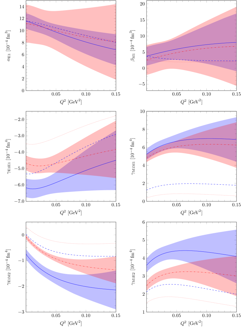
Figure 5: $Q^{2}$-dependence of the scalar and spin polarizabilites for the proton (dotted and dash-dotted lines) and the neutron (dashed and solid lines). The dotted and dashed lines correspond to the $\Delta$-less $\mathcal{O}(q^{4})$ results, whereas the dash-dotted and solid lines correspond to the $\Delta$-full $\mathcal{O}(\epsilon^{3}+q^{4})$ results. The bands indicate the theoretical truncation errors.

We also present the $Q^{2}$-dependence of several combined spin polarizabilites, for some of which the experimental data are available, see Fig. 6 (their limiting values for $Q^{2}=0$ are collected in Table 6). We observe no improvement as compared to Bernard et al. (2013) (pure $\mathcal{O}(\epsilon^{3})$ calculation) due to the inclusion of the $\mathcal{O}(q^{4})$ contributions. In fact, the description of $\gamma_{0}$ for the proton is even worse. A possible source of such a discrepancy could be a missing contribution of the $\Delta$-loop diagrams at order $\mathcal{O}(\epsilon^{4})$, as was suggested in Bernard et al. (2013). On the other hand, taking into account a much better description of the data in Lensky et al. (2014) (within the $\delta$-counting scheme) and the fact that the disagreement of our result with experiment for the value of $\gamma_{0}$ for the proton at $Q^{2}=0$ was caused by the large contribution from the induced electric $\gamma N\Delta$-coupling (as a $1/m$ effect), one may expect the improvement to be achieved after including the relevant higher-order $\gamma N\Delta$-vertices from the effective Lagrangian analogously to Lensky et al. (2014).

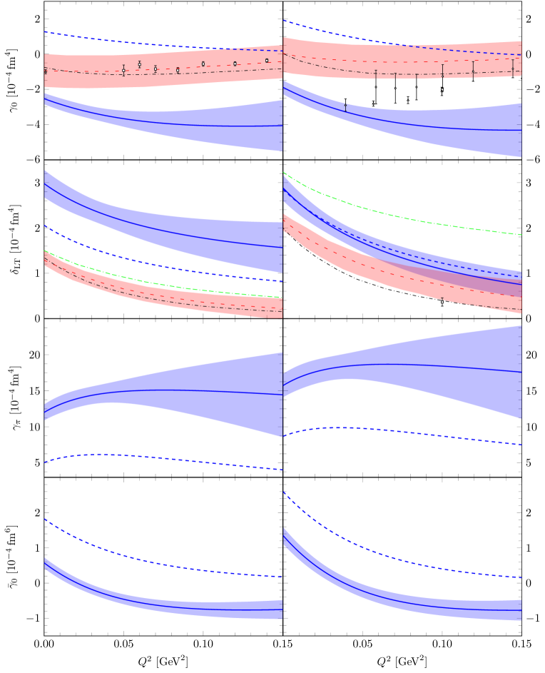
Figure 6: $Q^{2}$-dependencies of the forward polarizabilities $\gamma_{0}$ and $\delta_{\text{LT}}$, the backward polarizability $\gamma_{\pi}$ and the combined higher-order polarizability $\bar{\gamma}_{0}$ for the proton (left) and the neutron (right). The thick solid blue lines indicate our $\Delta$-full $\mathcal{O}(q^{4}+\epsilon^{3})$ calculations with a $1\sigma$ truncation error band corresponding to $68\%$ degree-of-belief intervals and the thick dashed blue lines show our $\Delta$-less $\mathcal{O}(q^{4})$ calculations. The red loosely dashed lines represent the NLO B$\chi$PT calculation from Alarcón et al. (2020b) with the red error bands. The black dash-dotted line presents the MAID model predictions from Drechsel et al. (2003) (proton) and Amarian et al. (2004) (neutron). The green double-dash-dotted line is the $\mathcal{O}(p^{4})$ calculation from Kao et al. (2003). Empirical data are: for $\gamma_{0}^{(p)}$ from Gryniuk et al. (2016) (triangle) and Prok et al. (2009) (squares); for $\gamma_{0}^{(n)}$ from Deur (2019) (preliminary, triangles), Amarian et al. (2004) (square) and Guler et al. (2015) (diamonds); for $\delta_{\text{LT}}^{(n)}$ from Amarian et al. (2004).

IV.5 Dynamical polarizabilities

One can also probe the electromagnetic structure of the nucleon by looking at dynamical (energy-dependent) polarizabilites that describe the response to the nucleon electromagnetic excitations at arbitrary energy. In Figs. 7, 8, we present the energy dependence of the dipole and spinless quadrupole polarizabilites up to the center-of-mass energy $\omega_{\text{CM}}=300$ MeV. For comparison, also shown are the results obtained using the $\delta$-counting scheme Lensky et al. (2015), the fixed-$t$ dispersion relations Hildebrandt et al. (2004), and the Computational Hadronic Model Aleksejevs and Barkanova (2013). The $1\sigma$ and $2\sigma$ truncation errors corresponding to $68\%$ and $95\%$ degree-of-belief intervals are shown as bands in the figures. Our results agree rather well with the ones of the fixed-$t$ dispersion relations at $\omega_{\text{CM}}=0$ (except for $\gamma_{E1M2}$). Therefore, it is natural to compare the two approaches at non-zero energies. As can be seen from the figures, the deviation of our results from those of the fixed-$t$ dispersion relations increases with energy, which may provide yet another indication that our theoretical errors are underestimated (as discussed in subsection IV.3), and the convergence of the small-scale expansion becomes slower $\omega_{\text{CM}}\gtrsim 150-200$ MeV. However, for $\alpha_{E2}$ a large discrepancy (beyond $2\sigma$) between the two theoretical frameworks is observed already for $\omega_{\text{CM}}\gtrsim 100-150$ MeV. This could be due to the aforementioned large induced electric $\gamma N\Delta$-coupling in our scheme, whose effect increases with energy.

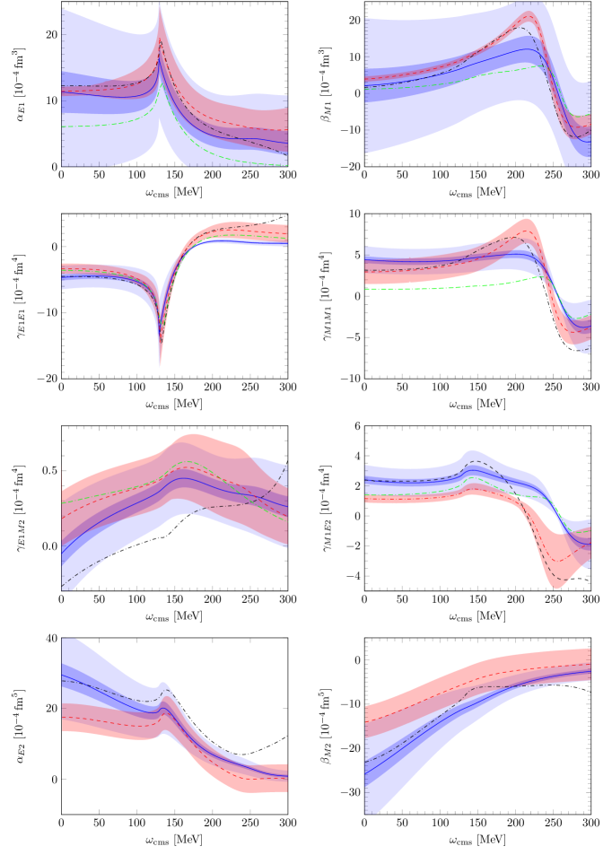
Figure 7: The $\omega$-dependence of the real parts of the dipole polarizabilities and the spinless quadrupole polarizabilites $\alpha_{\text{E2}}$ and $\beta_{\text{M2}}$ for the proton. The solid blue lines represent our $\Delta$-full $\mathcal{O}(q^{4}+\epsilon^{3})$ result. The inner (outer) blue bands stand for the $1\sigma$ ($2\sigma$) truncation error. The red dashed lines are the B$\chi$PT calculation Lensky et al. (2015) with the red error bands. The black dash-dotted lines correspond to the fixed-$t$ dispersion-relations calculation Hildebrandt et al. (2004) and the green double-dash-dotted lines correspond to the results of Aleksejevs and Barkanova (2013).

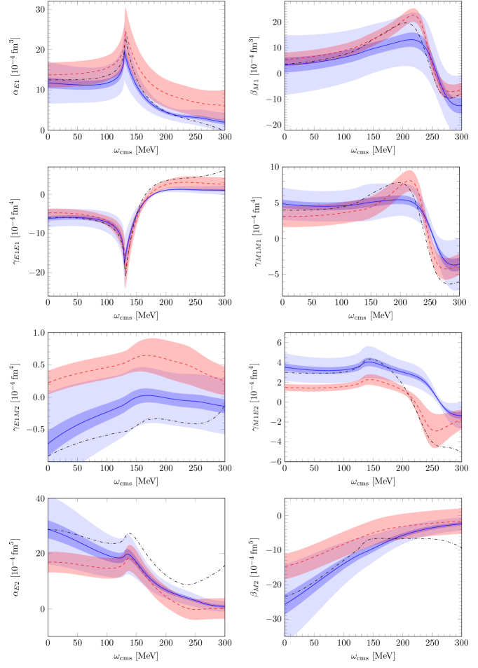
Figure 8: The $\omega$-dependence of the real parts of the dipole polarizabilities and the spinless quadrupole polarizabilites $\alpha_{\text{E2}}$ and $\beta_{\text{M2}}$ for the neutron. The solid blue lines represent our $\Delta$-full $\mathcal{O}(q^{4}+\epsilon^{3})$ result. The inner (outer) blue bands stand for the $1\sigma$ ($2\sigma$) truncation error. The red dashed lines are the B$\chi$PT calculation Lensky et al. (2015) with the red error bands. The black dash-dotted lines correspond to the fixed-$t$ dispersion-relations calculation Hildebrandt et al. (2004).

IV.6 Heavy-Baryon Expansion

In this subsection, we study the convergence of the $1/m$-expansion of our results (the nucleon-$\Delta$ mass difference $\Delta$ is kept finite and constant) obtained within the covariant framework. analyzing such an expansion we can test the efficiency of the heavy-baryon approach by reproducing some of its contributions appearing at higher orders. We present the $1/m$-expansion for the dipole scalar and spin polarizabilities in Tables 10-15 starting from the leading order (LO) static ($m^{0}$) results up to the order $1/m^{5}$ (N⁵LO). Obviously, the static results as well as the $1/m$-corrections to the leading-order terms coincide with the corresponding heavy-baryon calculations, see Bernard et al. (1995); Vijaya Kumar et al. (2000); Gellas et al. (2000); Hemmert et al. (1997).

$\alpha_{\text{E1}}^{(p)}$	$\phantom{-}q^{3}$	$\phantom{-}q^{4}$	$\phantom{-}\epsilon^{3}_{\text{Loop}}$	$\phantom{-}\epsilon^{3}_{\text{Tree}}$	Full		$\alpha_{\text{E1}}^{(n)}$	$\phantom{-}q^{3}$	$\phantom{-}q^{4}$	$\phantom{-}\epsilon^{3}_{\text{Loop}}$	$\phantom{-}\epsilon^{3}_{\text{Tree}}$	Full
$\operatorname{LO}$	$12.78$	$\phantom{1}8.86$	$\phantom{-}7.86$	$\phantom{-}\ldots$	$\phantom{-}29.50$		$\operatorname{LO}$	$12.78$	$\phantom{1}2.67$	$\phantom{-}7.86$	$\phantom{-}\ldots$	$\phantom{-}23.31$
$\operatorname{NLO}$	$\phantom{1}8.47$	$\phantom{1}8.86$	$\phantom{-}2.89$	$-5.60$	$\phantom{-}14.61$		$\operatorname{NLO}$	$\phantom{1}9.67$	$\phantom{1}2.67$	$\phantom{-}4.94$	$-5.60$	$\phantom{-}11.68$
$\operatorname{N}^{2}\!\operatorname{LO}$	$\phantom{1}6.60$	$\phantom{1}9.53$	$\phantom{-}0.97$	$-2.98$	$\phantom{-}14.13$		$\operatorname{N}^{2}\!\operatorname{LO}$	$\phantom{1}9.50$	$\phantom{1}3.22$	$\phantom{-}3.03$	$-2.98$	$\phantom{-}12.77$
$\operatorname{N}^{3}\!\operatorname{LO}$	$\phantom{1}7.01$	$\phantom{1}9.40$	$-1.03$	$-4.11$	$\phantom{-}11.26$		$\operatorname{N}^{3}\!\operatorname{LO}$	$\phantom{1}9.51$	$\phantom{1}3.10$	$\phantom{-}2.70$	$-4.11$	$\phantom{-}11.19$
$\operatorname{N}^{4}\!\operatorname{LO}$	$\phantom{1}7.04$	$\phantom{1}9.40$	$-1.33$	$-3.65$	$\phantom{-}11.46$		$\operatorname{N}^{4}\!\operatorname{LO}$	$\phantom{1}9.51$	$\phantom{1}3.09$	$\phantom{-}2.83$	$-3.65$	$\phantom{-}11.78$
$\operatorname{N}^{5}\!\operatorname{LO}$	$\phantom{1}7.04$	$\phantom{1}9.40$	$-1.49$	$-3.83$	$\phantom{-}11.12$		$\operatorname{N}^{5}\!\operatorname{LO}$	$\phantom{1}9.51$	$\phantom{1}3.09$	$\phantom{-}2.75$	$-3.83$	$\phantom{-}11.52$
Full	$\phantom{1}7.04$	$\phantom{1}9.40$	$-1.45$	$-3.78$	$\phantom{-}11.20$		Full	$\phantom{1}9.51$	$\phantom{1}3.09$	$\phantom{-}2.78$	$-3.78$	$\phantom{-}11.60$

Table 10: Numerical values for the $1/m$-expansion of $\alpha_{\text{E1}}$. Note that the $\epsilon^{3}_{\text{Tree}}$ only starts at NLO.

$\beta_{\text{M1}}^{(p)}$	$\phantom{-}q^{3}$	$\phantom{-}q^{4}$	$\phantom{-}\epsilon^{3}_{\text{Loop}}$	$\phantom{-}\epsilon^{3}_{\text{Tree}}$	Full		$\beta_{\text{M1}}^{(n)}$	$\phantom{-}q^{3}$	$\phantom{-}q^{4}$	$\phantom{-}\epsilon^{3}_{\text{Loop}}$	$\phantom{-}\epsilon^{3}_{\text{Tree}}$	Full
$\operatorname{LO}$	$\phantom{-}1.28$	$-12.33$	$\phantom{1}1.36$	$11.96$	$2.26$		$\operatorname{LO}$	$\phantom{-}1.28$	$-7.35$	$\phantom{1}1.36$	$11.96$	$7.24$
$\operatorname{NLO}$	$\phantom{-}0.56$	$-12.09$	$\phantom{1}1.61$	$11.96$	$2.04$		$\operatorname{NLO}$	$-0.88$	$-7.60$	$\phantom{1}0.34$	$11.96$	$3.83$
$\operatorname{N}^{2}\!\operatorname{LO}$	$-2.83$	$-13.75$	$\phantom{1}9.05$	$11.96$	$4.43$		$\operatorname{N}^{2}\!\operatorname{LO}$	$-1.11$	$-8.27$	$\phantom{1}1.28$	$11.96$	$3.85$
$\operatorname{N}^{3}\!\operatorname{LO}$	$-1.94$	$-13.23$	$\phantom{1}5.67$	$11.96$	$2.45$		$\operatorname{N}^{3}\!\operatorname{LO}$	$-1.10$	$-8.12$	$\phantom{1}0.69$	$11.96$	$3.43$
$\operatorname{N}^{4}\!\operatorname{LO}$	$-1.83$	$-13.14$	$\phantom{1}6.39$	$11.96$	$3.38$		$\operatorname{N}^{4}\!\operatorname{LO}$	$-1.10$	$-8.12$	$\phantom{1}1.09$	$11.96$	$3.83$
$\operatorname{N}^{5}\!\operatorname{LO}$	$-1.85$	$-13.16$	$\phantom{1}5.32$	$11.96$	$2.28$		$\operatorname{N}^{5}\!\operatorname{LO}$	$-1.10$	$-8.12$	$\phantom{1}0.90$	$11.96$	$3.64$
Full	$-1.85$	$-13.16$	$\phantom{1}5.54$	$11.96$	$2.50$		Full	$-1.10$	$-8.12$	$\phantom{1}0.96$	$11.96$	$3.70$

Table 11: Numerical values for the $1/m$-expansion of $\beta_{\text{M1}}$.

$\gamma_{\text{E1E1}}^{(p)}$	$\phantom{-}q^{3}$	$\phantom{-}q^{4}$	$\phantom{-}\epsilon^{3}_{\text{Loop}}$	$\phantom{-}\epsilon^{3}_{\text{Tree}}$	Full		$\gamma_{E1E1}^{(n)}$	$\phantom{-}q^{3}$	$\phantom{-}q^{4}$	$\phantom{-}\epsilon^{3}_{\text{Loop}}$	$\phantom{-}\epsilon^{3}_{\text{Tree}}$	Full
$\operatorname{LO}$	$-5.81$	$\phantom{-}\ldots$	$\phantom{-}0.60$	$\phantom{-}\ldots$	$-5.22$		$\operatorname{LO}$	$-5.81$	$\phantom{-}\ldots$	$\phantom{-}0.60$	$\phantom{-}\ldots$	$-5.22$
$\operatorname{NLO}$	$-1.38$	$\phantom{-}\ldots$	$\phantom{-}0.96$	$-0.63$	$-1.05$		$\operatorname{NLO}$	$-4.34$	$\phantom{-}\ldots$	$\phantom{-}0.66$	$-0.63$	$-4.31$
$\operatorname{N}^{2}\!\operatorname{LO}$	$-3.03$	$\phantom{-}0.20$	$-0.63$	$-1.22$	$-4.68$		$\operatorname{N}^{2}\!\operatorname{LO}$	$-4.83$	$-0.37$	$\phantom{-}0.84$	$-1.22$	$-5.58$
$\operatorname{N}^{3}\!\operatorname{LO}$	$-3.57$	$-0.11$	$-1.41$	$-1.02$	$-6.11$		$\operatorname{N}^{3}\!\operatorname{LO}$	$-4.86$	$-0.49$	$\phantom{-}0.07$	$-1.02$	$-6.30$
$\operatorname{N}^{4}\!\operatorname{LO}$	$-3.47$	$-0.02$	$\phantom{-}0.07$	$-1.08$	$-4.50$		$\operatorname{N}^{4}\!\operatorname{LO}$	$-4.86$	$-0.46$	$\phantom{-}0.26$	$-1.08$	$-6.15$
$\operatorname{N}^{5}\!\operatorname{LO}$	$-3.46$	$-0.01$	$-0.13$	$-1.06$	$-4.66$		$\operatorname{N}^{5}\!\operatorname{LO}$	$-4.86$	$-0.46$	$\phantom{-}0.23$	$-1.06$	$-6.16$
Full	$-3.46$	$-0.01$	$-0.11$	$-1.07$	$-4.65$		Full	$-4.86$	$-0.46$	$\phantom{-}0.22$	$-1.07$	$-6.17$

Table 12: Numerical values for the $1/m$-expansion of $\gamma_{\text{E1E1}}$. The dots mark entries that do not exist e.g. the $\epsilon^{3}_{\text{Tree}}$ starts at NLO and therefore does not have a LO contribution.

$\gamma_{\text{M1M1}}^{(p)}$	$\phantom{-}q^{3}$	$\phantom{-}q^{4}$	$\phantom{-}\epsilon^{3}_{\text{Loop}}$	$\phantom{-}\epsilon^{3}_{\text{Tree}}$	Full		$\gamma_{M1M1}^{(n)}$	$\phantom{-}q^{3}$	$\phantom{-}q^{4}$	$\phantom{-}\epsilon^{3}_{\text{Loop}}$	$\phantom{-}\epsilon^{3}_{\text{Tree}}$	Full
$\operatorname{LO}$	$-1.16$	$\phantom{-}\ldots$	$\phantom{-}0.21$	$\phantom{-}4.03$	$\phantom{-}3.08$		$\operatorname{LO}$	$-1.16$	$\phantom{-}\ldots$	$\phantom{-}0.21$	$\phantom{-}4.03$	$\phantom{-}3.08$
$\operatorname{NLO}$	$\phantom{-}1.39$	$\phantom{-}1.93$	$-0.12$	$\phantom{-}3.40$	$\phantom{-}6.59$		$\operatorname{NLO}$	$\phantom{-}0.31$	$\phantom{-}2.05$	$-0.27$	$\phantom{-}3.40$	$\phantom{-}5.49$
$\operatorname{N}^{2}\!\operatorname{LO}$	$\phantom{-}0.52$	$\phantom{-}1.24$	$\phantom{-}2.21$	$\phantom{-}3.89$	$\phantom{-}7.85$		$\operatorname{N}^{2}\!\operatorname{LO}$	$-0.13$	$\phantom{-}1.56$	$\phantom{-}0.78$	$\phantom{-}3.89$	$\phantom{-}6.11$
$\operatorname{N}^{3}\!\operatorname{LO}$	$-0.37$	$\phantom{-}0.19$	$-0.44$	$\phantom{-}3.87$	$\phantom{-}3.26$		$\operatorname{N}^{3}\!\operatorname{LO}$	$-0.17$	$\phantom{-}1.39$	$\phantom{-}0.04$	$\phantom{-}3.87$	$\phantom{-}5.13$
$\operatorname{N}^{4}\!\operatorname{LO}$	$-0.15$	$\phantom{-}0.46$	$\phantom{-}0.81$	$\phantom{-}3.84$	$\phantom{-}4.96$		$\operatorname{N}^{4}\!\operatorname{LO}$	$-0.17$	$\phantom{-}1.42$	$\phantom{-}0.23$	$\phantom{-}3.84$	$\phantom{-}5.33$
$\operatorname{N}^{5}\!\operatorname{LO}$	$-0.12$	$\phantom{-}0.50$	$\phantom{-}0.39$	$\phantom{-}3.86$	$\phantom{-}4.62$		$\operatorname{N}^{5}\!\operatorname{LO}$	$-0.17$	$\phantom{-}1.42$	$\phantom{-}0.05$	$\phantom{-}3.86$	$\phantom{-}5.16$
Full	$-0.13$	$\phantom{-}0.49$	$\phantom{-}0.58$	$\phantom{-}3.85$	$\phantom{-}4.80$		Full	$-0.17$	$\phantom{-}1.42$	$\phantom{-}0.12$	$\phantom{-}3.85$	$\phantom{-}5.22$

Table 13: Numerical values for the $1/m$-expansion of $\gamma_{\text{M1M1}}$. The dots mark entries that do not exist e.g. the $q^{4}$ starts at NLO and therefore does not have a LO contribution.

$\gamma_{\text{E1M2}}^{(p)}$	$\phantom{-}q^{3}$	$\phantom{-}q^{4}$	$\phantom{-}\epsilon^{3}_{\text{Loop}}$	$\phantom{-}\epsilon^{3}_{\text{Tree}}$	Full		$\gamma_{E1M2}^{(n)}$	$\phantom{-}q^{3}$	$\phantom{-}q^{4}$	$\phantom{-}\epsilon^{3}_{\text{Loop}}$	$\phantom{-}\epsilon^{3}_{\text{Tree}}$	Full
$\operatorname{LO}$	$\phantom{-}1.16$	$\phantom{-}\ldots$	$-0.21$	$\phantom{-}\ldots$	$\phantom{-}0.95$		$\operatorname{LO}$	$\phantom{-}1.16$	$\phantom{-}\ldots$	$-0.21$	$\phantom{-}\ldots$	$\phantom{-}0.95$
$\operatorname{NLO}$	$\phantom{-}0.22$	$\phantom{-}\ldots$	$\phantom{-}0.01$	$-0.63$	$-0.40$		$\operatorname{NLO}$	$\phantom{-}0.49$	$\phantom{-}\ldots$	$\phantom{-}0.04$	$-0.63$	$-0.09$
$\operatorname{N}^{2}\!\operatorname{LO}$	$\phantom{-}0.57$	$\phantom{-}0.03$	$\phantom{-}1.43$	$-0.92$	$\phantom{-}1.11$		$\operatorname{N}^{2}\!\operatorname{LO}$	$\phantom{-}0.60$	$-0.43$	$\phantom{-}0.21$	$-0.92$	$-0.54$
$\operatorname{N}^{3}\!\operatorname{LO}$	$\phantom{-}0.54$	$-0.36$	$\phantom{-}0.84$	$-0.88$	$\phantom{-}0.15$		$\operatorname{N}^{3}\!\operatorname{LO}$	$\phantom{-}0.61$	$-0.63$	$\phantom{-}0.27$	$-0.88$	$-0.64$
$\operatorname{N}^{4}\!\operatorname{LO}$	$\phantom{-}0.56$	$-0.26$	$\phantom{-}0.05$	$-0.88$	$-0.52$		$\operatorname{N}^{4}\!\operatorname{LO}$	$\phantom{-}0.61$	$-0.59$	$\phantom{-}0.03$	$-0.88$	$-0.84$
$\operatorname{N}^{5}\!\operatorname{LO}$	$\phantom{-}0.57$	$-0.25$	$\phantom{-}0.70$	$-0.88$	$\phantom{-}0.14$		$\operatorname{N}^{5}\!\operatorname{LO}$	$\phantom{-}0.61$	$-0.59$	$\phantom{-}0.16$	$-0.88$	$-0.70$
Full	$\phantom{-}0.57$	$-0.25$	$\phantom{-}0.48$	$-0.88$	$-0.08$		Full	$\phantom{-}0.61$	$-0.59$	$\phantom{-}0.11$	$-0.88$	$-0.75$

Table 14: Numerical values for the $1/m$-expansion of $\gamma_{\text{E1M2}}$. The dots mark entries that do not exist e.g. the $\epsilon^{3}_{\text{Tree}}$ starts at NLO and therefore does not have a LO contribution.

$\gamma_{\text{M1E2}}^{(p)}$	$\phantom{-}q^{3}$	$\phantom{-}q^{4}$	$\phantom{-}\epsilon^{3}_{\text{Loop}}$	$\phantom{-}\epsilon^{3}_{\text{Tree}}$	Full		$\gamma_{M1E2}^{(n)}$	$\phantom{-}q^{3}$	$\phantom{-}q^{4}$	$\phantom{-}\epsilon^{3}_{\text{Loop}}$	$\phantom{-}\epsilon^{3}_{\text{Tree}}$	Full
$\operatorname{LO}$	$\phantom{-}1.16$	$\phantom{-}\ldots$	$-0.21$	$\phantom{-}\ldots$	$\phantom{-}0.95$		$\operatorname{LO}$	$\phantom{-}1.16$	$\phantom{-}\ldots$	$-0.21$	$\phantom{-}\ldots$	$\phantom{-}0.95$
$\operatorname{NLO}$	$\phantom{-}0.76$	$\phantom{-}1.03$	$-0.11$	$\phantom{-}1.89$	$\phantom{-}3.56$		$\operatorname{NLO}$	$\phantom{-}1.30$	$\phantom{-}0.96$	$-0.08$	$\phantom{-}1.89$	$\phantom{-}4.06$
$\operatorname{N}^{2}\!\operatorname{LO}$	$\phantom{-}0.89$	$\phantom{-}0.66$	$-1.32$	$\phantom{-}1.59$	$\phantom{-}1.82$		$\operatorname{N}^{2}\!\operatorname{LO}$	$\phantom{-}1.36$	$\phantom{-}0.87$	$-0.33$	$\phantom{-}1.59$	$\phantom{-}3.48$
$\operatorname{N}^{3}\!\operatorname{LO}$	$\phantom{-}0.98$	$\phantom{-}0.52$	$-1.02$	$\phantom{-}1.82$	$\phantom{-}2.31$		$\operatorname{N}^{3}\!\operatorname{LO}$	$\phantom{-}1.37$	$\phantom{-}0.73$	$-0.25$	$\phantom{-}1.82$	$\phantom{-}3.67$
$\operatorname{N}^{4}\!\operatorname{LO}$	$\phantom{-}0.95$	$\phantom{-}0.56$	$-0.80$	$\phantom{-}1.71$	$\phantom{-}2.42$		$\operatorname{N}^{4}\!\operatorname{LO}$	$\phantom{-}1.36$	$\phantom{-}0.76$	$-0.26$	$\phantom{-}1.71$	$\phantom{-}3.57$
$\operatorname{N}^{5}\!\operatorname{LO}$	$\phantom{-}0.95$	$\phantom{-}0.56$	$-0.86$	$\phantom{-}1.76$	$\phantom{-}2.40$		$\operatorname{N}^{5}\!\operatorname{LO}$	$\phantom{-}1.36$	$\phantom{-}0.76$	$-0.29$	$\phantom{-}1.76$	$\phantom{-}3.59$
Full	$\phantom{-}0.95$	$\phantom{-}0.56$	$-0.79$	$\phantom{-}1.74$	$\phantom{-}2.47$		Full	$\phantom{-}1.36$	$\phantom{-}0.76$	$-0.27$	$\phantom{-}1.74$	$\phantom{-}3.59$

Table 15: Numerical values for the $1/m$-expansion of $\gamma_{\text{M1E2}}$. The dots mark entries that do not exist e.g. the $\epsilon^{3}_{\text{Tree}}$ starts at NLO and therefore does not have a LO contribution.

We first consider the convergence of the $1/m$-expansion of the individual contributions from the $q^{3}$-, $q^{4}$- and $\epsilon^{3}$-loop diagrams, and from the $\Delta$-tree-level terms. In general, the convergence is rather slow. The most rapid convergence is observed for the $q^{3}$- and $q^{4}$-loops. Sometimes (e.g. for $\alpha_{E1}$, $\gamma_{M1E2}$), the expanded value approaches the “exact” one already at NLO-N²LO. In other cases, the expanded values oscillate at lower $1/m$-orders, especially when the resulting value is small due to cancellations among various diagrams. It is natural to expect a slower convergence for the diagrams with $\Delta$-lines as the formal expansion parameter $\Delta/m$ is roughly twice as large as $M/m$. Nevertheless, the expansion for the tree-$\Delta$-graphs converges, in general, only slightly worse than the $\pi N$-loops ($\beta_{M1}$ is accidentally $m$-independent). On the other hand, for the $\Delta\pi$-loops, the convergence is very poor. This set of diagrams comprises loops with one, two and three $\Delta$-lines, and cancellations among them occur quite often. Some of the values strongly oscillate and one hardly sees a sign of convergence even at N⁵LO, e.g. for $\gamma_{M1M1}$, $\gamma_{E1M2}$.

Nevertheless, we have checked that the $1/m$-expansion converges in principle (formally) for all diagrams. This is illustrated in Figs. 9, 10, where the logarithm of the remainder in the $1/m$-series is plotted against the order of expansion. As one can see from the plots, the expanded $\Delta$-loops approach their unexpanded values very slowly, making such an expansion impractical. Note that contributions of the $\Delta$-loops are smaller for the spin-dependent polarizabilities.

We now consider the $1/m$-expansion of the sum of all contributions to the nucleon polarizabilities. As one can see in Tables 10, 11, the electric and magnetic scalar polarizabilities at NLO agree rather well with the unexpanded values (for the absolute difference is large but the relative difference is small), while the individual contributions in some cases strongly oscillate. Such an agreement is accidental. Moreover, e.g. the $\beta^{(}p)_{M1}$ at N²LO deviates significantly from the full result and approaches it again after several oscillations. Nevertheless, these effects can be compensated by a redefinition of the $q^{4}$ contact terms.

The situation is different for the spin-dependent polarizabilities, where the NLO values in most cases deviate rather strongly from the unexpanded result, see Tables 12-15. It should be emphasized that these differences can be absorbed into contact terms only at order $q^{5}$.

Summarizing, we conclude that the $1/m$-expansion (and, hence, the heavy-baryon scheme) is rather inefficient for calculating nucleon polarizabilites in the $\Delta$-full approach, which is in line with the results of the heavy-baryon calculations mentioned above. On the other hand, the small-scale expansion seems to converge reasonably well.

Figure 9: Logarithmic difference of the absolute value between the HB-expanded contributions and the final, non-expanded value for the spin-independent and spin-dependent dipole polarizabilities of the proton. $i$ stands for the $i$-th order in the HB expansion. The black squares represent the $q^{3}$ contribution, the red triangles represent the $q^{4}$ contribution, the blue circles represent the $\epsilon^{3}$-loop contribution and the green diamonds represent the $\epsilon^{3}$-tree contributions. The dashed lines stand for the corresponding linear regression.

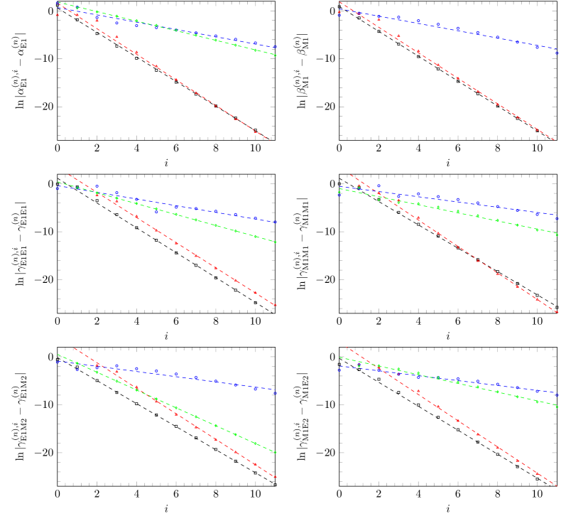
Figure 10: Logarithmic difference of the absolute value between the HB-expanded contributions and the final, non-expanded value for the spin-independent and spin-dependent dipole polarizabilities of the neutron. $i$ stands for the $i$-th order in the HB expansion. The black squares represent the $q^{3}$ contribution, the red triangles represent the $q^{4}$ contribution, the blue circles represent the $\epsilon^{3}$-loop contribution and the green diamonds represent the $\epsilon^{3}$-tree contributions. The dashed lines stand for the corresponding linear regression.

V Summary and outlook

In this work, we have presented various nucleon polarizabilities obtained within covariant chiral perturbation theory with explicit $\Delta$(1232) degrees of freedom, calculated up to order $\mathcal{O}(\epsilon^{3}+q^{4})$ in the small-scale expansion. The theoretical errors were estimated by combining the uncertainties of the input parameters and the errors due to the truncation of the small-scale expansion calculated using a Bayesian model. The results were compared with the $\Delta$-less approach at order $\mathcal{O}(q^{3})$ and $\mathcal{O}(q^{4})$, as well as with the empirical values and other theoretical approaches (in particular, with the $\delta$-counting $\Delta$-full scheme and the fixed-$t$ dispersion-relations method).

The general conclusion of this study is that the $\Delta$-full scheme that we adopt is quite efficient for analyzing the nucleon polarizabilites. It shows reasonable convergence, and the obtained results agree well with experiment and the fixed-$t$ dispersion-relations values. The results obtained in the $\Delta$-less approach are considerably worse both from the point of view of convergence and agreement with experiment.

The scalar dipole polarizabilites were used as an input to adjust four low energy constants appearing at order $\mathcal{O}(q^{4})$ in the effective Lagrangian. Therefore, we were not concerned with the issue of convergence for these quantities (although the convergence is far from being satisfactory).

Our predictions for the dipole spin polarizabilites $\gamma_{E1E1}$, $\gamma_{E1M2}$, $\gamma_{M1E2}$ obtained in the $\Delta$-full scheme agree with experimental values of Martel et al. (2015) and are slightly larger for $\gamma_{M1M1}$. The agreement is somewhat worse with the analysis of the recent MAMI experiment Martel et al. (2015). The same pattern is observed in the comparison with the fixed-$t$ dispersion-relations results. On the other hand, the predictions for the forward and backward spin polarizabilites $\gamma_{0}$ and $\gamma+\pi$ differ noticeably from the empirical values. Such a deviation can be explained by a sizable contributions of the “induced” electric $\gamma N\Delta$-coupling observed for these linear combinations. This effect if formally suppressed by a factor of $1/m$, but numerically it turns out to be sizable. In the $\delta$-counting scheme of Lensky et al. (2015), the electric $\gamma N\Delta$-coupling constant is adjusted to data and appears to be rather small. This is an indication that including higher-order $\Delta$-pole graphs in our scheme might improve the results.

Due to small contributions of the $q^{4}$-loops to spin polarizabilites, a rather rapid convergence is achieved for all of them.

We have also analyzed several higher-order polarizabilites. A nice convergence rate is observed for all polarizabilites calculated within the $\Delta$-full scheme. This is, however, not the case for the higher-order scalar polarizabilites calculated in the $\Delta$-less approach. This pattern can be understood in terms of the $\Delta$-resonance saturation of the low-energy constants $c_{2}$ and $c_{3}$. The main effect of the explicit treatment of the $\Delta$ is that some parts of the $q^{4}$-loops are shifted to the $\epsilon^{3}$-loops.

For the scalar quadrupole and dipole-dispersive polarizabilites, our predictions agree with the results of the fixed-$t$ dispersion-relations approach. However, our results differ noticeably from the ones obtained in the $\delta$-counting scheme. This difference is caused not only by the $q^{4}$-loop contributions, but also by the $\epsilon^{3}$-loops with multiple $\Delta$-lines, which contribute at higher orders in the $\delta$-counting scheme. This points to the importance of such terms also for higher-order polarizabilites.

We also studied the $Q^{2}$-dependence of the nucleon polarizabilites by considering generalized scalar and spin polarizabilities. We found that the $Q^{2}$-dependence of the magnetic scalar polarizabilites is significantly different in the $\Delta$-full and the $\Delta$-less approach. We also observed a substantial deviation of the $\mathcal{O}(\epsilon^{3}+q^{4})$ results for the $Q^{2}$-dependent polarizabilities $\gamma_{0}$ for the proton and for the neutron as well as $\delta_{\text{LT}}$ for the neutron from the available experimental data and no improvement compared to the $\mathcal{O}(\epsilon^{3})$-results. We expect that taking into account the $\mathcal{O}(\epsilon^{4})$ terms (in particular the tree-level graphs) might improve the description of the data.

An alternative way to study the electromagnetic structure of the nucleon is to consider dynamical (energy-dependent) polarizabilites. We have analyzed the energy dependence of the dipole and spinless quadrupole polarizabilites and compared them with other theoretical investigations. In particular, we observed a rather large deviation from the fixed-$t$ dispersion-relations approach at energies $\omega_{\text{CM}}\gtrsim 150-200$ MeV (in some cases for $\omega_{\text{CM}}\gtrsim 100$ MeV), which indicates the slow convergence of the small-scale expansion in that energy region.

Finally, we have analyzed the convergence of the $1/m$-expansion of the results obtained in the covariant calculation for various polarizabilites. Such an scheme allows one to see how reliable the heavy-baryon expansion is for the evaluation of the nucleon polarizabilites. We considered the expansion up to N⁵LO. Our conclusion is that the heavy-baryon expansion is not efficient for calculating nucleon polarizabilites in the $\Delta$-full approach. Nevertheless, the small-scale expansion seems to converge reasonably well.

A natural extension of the current work towards increasing accuracy of the results follows from the discussion above. We expect a better accuracy and a better agreement with the experimental data after including the $\Delta$-tree-level graphs of order $\mathcal{O}(\epsilon^{4})$ with the electric $\gamma N\Delta$-coupling as well as the $\mathcal{O}(\epsilon^{4})$-loop diagrams, that is performing a complete $\mathcal{O}(\epsilon^{4})$ calculation.

Appendix A $q^{3}$-Values

The analytic expressions for $\alpha_{\text{E1}}$, $\beta_{\text{M1}}$, $\alpha_{\text{E2}}$, $\beta_{\text{M2}}$ and a linear combination of the spin-dependent first order polarizabilities for both proton and neutron were already calculated in Lensky et al. (2015) but are also given here for completeness. For convenience we define $\Xi_{2}=\Xi\left(m^{2},m,M\right)/(\mu^{2}-4)$ where $\mu=M/m$, $\Xi_{1}=\ln\left(\mu\right)$ and

$$\Xi(p^{2},m_{1},m_{2}) =\frac{1}{p^{2}}\sqrt{\lambda(m_{1}^{2},m_{2}^{2},p^{2})}\ln\left(\frac{m_{1}^{2}+m_{2}^{2}+\sqrt{\lambda(m_{1}^{2},m_{2}^{2},p^{2})}-p^{2}}{2m_{1}m_{2}}\right)\,,$$

$$\lambda(a,b,c) =a^{2}+b^{2}+c^{2}-2ab-2bc-2ac\,.$$ (33)

A.1 Proton values

A.1.1 Spin-independent first order polarizabilities

$$\alpha_{\text{E1}}^{(p)}=\;\frac{e^{2}g_{A}^{2}}{192\pi^{3}F^{2}\mu^{2}\left(\mu^{2}-4\right)^{2}m}\left[\vphantom{\frac{e}{m}}2\left(-9\mu^{10}+110\mu^{8}-479\mu^{6}+870\mu^{4}-590\mu^{2}+80\right)\Xi_{2}\right.$$

$$\;\;\;\;\left.\left.+\left(-18\mu^{8}+157\mu^{6}-407\mu^{4}+304\mu^{2}\right)\vphantom{\frac{e}{m}}\right]+\frac{e^{2}g_{A}^{2}\left(9\mu^{4}-20\mu^{2}+9\right)\Xi_{1}}{96\pi^{3}F^{2}m}\right.\,,$$

$$\beta_{\text{M1}}^{(p)}=-\frac{e^{2}g_{A}^{2}}{192\pi^{3}F^{2}\mu^{2}\left(\mu^{2}-4\right)m}\left[\vphantom{\frac{e}{m}}2\left(27\mu^{8}-212\mu^{6}+471\mu^{4}-246\mu^{2}+2\right)\Xi_{2}\right.$$

$$\;\;\;\;\left.\left.-\left(54\mu^{6}-235\mu^{4}+127\mu^{2}\right)\vphantom{\frac{e}{m}}\right]+\frac{e^{2}g_{A}^{2}\left(27\mu^{4}-50\mu^{2}+9\right)\Xi_{1}}{96\pi^{3}F^{2}m}\right.\,.$$

A.1.2 Spin-independent second order polarizabilities

$$\alpha_{\text{E2}}^{(p)}=-\frac{e^{2}g_{A}^{2}}{480\pi^{3}F^{2}\mu^{4}\left(\mu^{2}-4\right)^{3}m^{3}}\left[\vphantom{\frac{e}{m}}\left(450\mu^{14}-7341\mu^{12}+16584\mu^{10}-143010\mu^{8}\right.\right.\vphantom{\frac{e}{m}}$$

$$\;\;\;\;\left.\left.+212940\mu^{6}-132300\mu^{4}+18624\mu^{2}+1344\right)\Xi_{2}-450\mu^{12}-5766\mu^{10}+26437\mu^{8}\right.\vphantom{\frac{e}{m}}$$

$$\;\;\;\;\left.-50449\mu^{6}+34592\mu^{4}-3536\mu^{2}\vphantom{\frac{e}{m}}\right]+\frac{e^{2}g_{A}^{2}\Xi_{1}}{160\pi^{3}F^{2}m^{3}}\left(150\mu^{4}-347\mu^{2}+170\right)\,,$$

$$\beta_{\text{M2}}^{(p)}=-\frac{e^{2}g_{A}^{2}}{480\pi^{3}F^{2}\mu^{4}\left(\mu^{2}-4\right)^{2}m^{3}}\left[\vphantom{\frac{e}{m}}\left(990\mu^{12}-11781\mu^{10}+49020\mu^{8}-81330\mu^{6}\right.\right.\vphantom{\frac{e}{m}}$$

$$\;\;\;\;\left.\left.+43020\mu^{4}-2700\mu^{2}+144\right)\Xi_{2}+990\mu^{10}-8316\mu^{8}+20000\mu^{6}-11137\mu^{4}+92\mu^{2}\vphantom{\frac{e}{m}}\right]$$

$$\;\;\;\;+\frac{e^{2}g_{A}^{2}\Xi_{1}}{160\pi^{3}F^{2}m^{3}}\left(330\mu^{4}-627\mu^{2}+170\right)\,,$$

$$\alpha_{\text{E1}\nu}^{(p)}=\;\frac{e^{2}g_{A}^{2}}{5760\pi^{3}F^{2}\mu^{4}\left(\mu^{2}-4\right)^{4}m^{3}}\left[\vphantom{\frac{e}{m}}\left(-5130\mu^{16}+102987\mu^{14}-841656\mu^{12}\right.\right.\vphantom{\frac{e}{m}}$$

$$\;\;\;\;\left.\left.+3561462\mu^{10}-8161020\mu^{8}+9522420\mu^{6}-4534128\mu^{4}+397824\mu^{2}+6912\right)\Xi_{2}\right.\vphantom{\frac{e}{m}}$$

$$\;\;\;\;\left.-5130\mu^{14}+85032\mu^{12}-544482\mu^{10}+1658251\mu^{8}-2335148\mu^{6}+1156768\mu^{4}\right.\vphantom{\frac{e}{m}}$$

$$\;\;\;\;\left.-45504\mu^{2}\vphantom{\frac{e}{m}}\right]+\frac{e^{2}g_{A}^{2}\Xi_{1}}{1920\pi^{3}F^{2}m^{3}}\left(1710\mu^{4}-3549\mu^{2}+1210\right)\,,$$

$$\beta_{\text{M1}\nu}^{(p)}=-\frac{e^{2}g_{A}^{2}}{1920\pi^{3}F^{2}\mu^{4}\left(\mu^{2}-4\right)^{3}m^{3}}\left[\vphantom{\frac{e}{m}}\left(1890\mu^{14}-30129\mu^{12}+184876\mu^{10}-538370\mu^{8}\right.\right.\vphantom{\frac{e}{m}}$$

$$\;\;\;\;\left.\left.+730660\mu^{6}-374140\mu^{4}+33056\mu^{2}+896\right)\Xi_{2}+1890\mu^{12}-23514\mu^{10}+102731\mu^{8}\right.\vphantom{\frac{e}{m}}$$

$$\;\;\;\;\left.-178873\mu^{6}+96560\mu^{4}-4032\mu^{2}\vphantom{\frac{e}{m}}\right]+\frac{e^{2}g_{A}^{2}\Xi_{1}}{1920\pi^{3}F^{2}m^{3}}\left(1890\mu^{4}-3669\mu^{2}+1210\right)\,.$$

A.1.3 Spin-dependent first order polarizabilities

$$\gamma_{\text{E1E1}}^{(p)}=\;\frac{e^{2}g_{A}^{2}}{384\pi^{3}F^{2}\mu^{2}\left(\mu^{2}-4\right)^{2}m^{2}}\left[\vphantom{\frac{e}{m}}2\left(-9\mu^{10}+134\mu^{8}-739\mu^{6}+1790\mu^{4}-1650\mu^{2}\right.\right.\vphantom{\frac{e}{m}}$$

$$\;\;\;\;\left.\left.+264\right)\Xi_{2}-\left(18\mu^{8}-205\mu^{6}+764\mu^{4}-900\mu^{2}+80\right)\vphantom{\frac{e}{m}}\right]+\frac{e^{2}g_{A}^{2}\Xi_{1}}{192\pi^{3}F^{2}m^{2}}\left(9\mu^{4}\right.\vphantom{\frac{e}{m}}$$

$$\;\;\;\;\left.\left.-44\mu^{2}+29\right)\right.\,,$$

$$\gamma_{\text{M1M1}}^{(p)}=\;\frac{e^{2}g_{A}^{2}}{384\pi^{3}F^{2}\mu^{2}\left(\mu^{2}-4\right)^{2}m^{2}}\left[\vphantom{\frac{e}{m}}2\left(-63\mu^{10}+744\mu^{8}-3059\mu^{6}+4970\mu^{4}-2534\mu^{2}\right.\right.\vphantom{\frac{e}{m}}$$

$$\;\;\;\;\left.\left.+152\right)\Xi_{2}-\left(126\mu^{8}-1047\mu^{6}+2462\mu^{4}-1308\mu^{2}+16\right)\vphantom{\frac{e}{m}}\right]+\frac{e^{2}g_{A}^{2}\Xi_{1}}{192\pi^{3}F^{2}m^{2}}\left(63\mu^{4}\right.\vphantom{\frac{e}{m}}$$

$$\;\;\;\;\left.\left.-114\mu^{2}+29\right)\right.\,,$$

$$\gamma_{\text{E1M2}}^{(p)}=-\frac{e^{2}g_{A}^{2}}{384\pi^{3}F^{2}\mu^{2}\left(\mu^{2}-4\right)^{2}m^{2}}\left[\vphantom{\frac{e}{m}}2\left(\left(3\left(\mu^{2}-5\right)\left(3\mu^{4}-19\mu^{2}+34\right)\mu^{2}+46\right)\mu^{2}\right.\right.\vphantom{\frac{e}{m}}$$

$$\;\;\;\;\left.\left.+56\right)\Xi_{2}+\left(-18\mu^{8}+141\mu^{6}-284\mu^{4}+4\mu^{2}+16\right)\vphantom{\frac{e}{m}}\right]+\frac{e^{2}g_{A}^{2}\Xi_{1}}{64\pi^{3}F^{2}m^{2}}\left(3\mu^{4}-4\mu^{2}-1\right)\,,$$

$$\gamma_{\text{M1E2}}^{(p)}=\;\frac{e^{2}g_{A}^{2}}{384\pi^{3}F^{2}\mu^{2}\left(\mu^{2}-4\right)m^{2}}\left[\vphantom{\frac{e}{m}}2\left(9\mu^{8}-68\mu^{6}+141\mu^{4}-66\mu^{2}+6\right)\Xi_{2}+\left(18\mu^{6}\right.\right.\vphantom{\frac{e}{m}}$$

$$\;\;\;\;\left.\left.-73\mu^{4}+30\mu^{2}-4\right)\vphantom{\frac{e}{m}}\right]-\frac{e^{2}g_{A}^{2}\Xi_{1}}{192\pi^{3}F^{2}m^{2}}\left(9\mu^{4}-14\mu^{2}+3\right)\,.$$

A.1.4 Spin-dependent second order polarizabilities

$$\gamma_{\text{E2E2}}^{(p)}=-\frac{e^{2}g_{A}^{2}}{138240\pi^{3}F^{2}\mu^{4}\left(\mu^{2}-4\right)^{3}m^{4}}\left[\vphantom{\frac{e}{m}}\left(6030\mu^{14}-107814\mu^{12}+764796\mu^{10}\right.\right.\vphantom{\frac{e}{m}}$$

$$\;\;\;\;\left.\left.-2694300\mu^{8}+4759500\mu^{6}-3591840\mu^{4}+577056\mu^{2}+36096\right)\Xi_{2}+6030\mu^{12}\right.\vphantom{\frac{e}{m}}$$

$$\;\;\;\;\left.-86709\mu^{10}+461861\mu^{8}-1079504\mu^{6}+954200\mu^{4}-100864\mu^{2}-3328\vphantom{\frac{e}{m}}\right]$$

$$\;\;+\frac{e^{2}g_{A}^{2}\Xi_{1}}{23040\pi^{3}F^{2}m^{4}}\left(1005\mu^{4}-3899\mu^{2}+2530\right)\,,$$

$$\gamma_{\text{M2M2}}^{(p)}=-\frac{e^{2}g_{A}^{2}}{138240\pi^{3}F^{2}\mu^{4}\left(\mu^{2}-4\right)^{3}m^{4}}\left[\vphantom{\frac{e}{m}}\left(29250\mu^{14}-462354\mu^{12}+2802636\mu^{10}\right.\right.\vphantom{\frac{e}{m}}$$

$$\;\;\;\;\left.\left.-8007300\mu^{8}+10510020\mu^{6}-5011200\mu^{4}+379296\mu^{2}+7296\right)\Xi_{2}+29250\mu^{12}\right.\vphantom{\frac{e}{m}}$$

$$\;\;\;\;\left.-359979\mu^{10}+1545103\mu^{8}-2601080\mu^{6}+1278024\mu^{4}-40480\mu^{2}-256\vphantom{\frac{e}{m}}\right]$$

$$\;\;+\frac{e^{2}g_{A}^{2}\Xi_{1}}{23040\pi^{3}F^{2}m^{4}}\left(4875\mu^{4}-8809\mu^{2}+2530\right)\,,$$

$$\gamma_{\text{E2M3}}^{(p)}=\;\frac{e^{2}g_{A}^{2}}{69120\pi^{3}F^{2}\mu^{4}\left(\mu^{2}-4\right)^{3}m^{4}}\left[\vphantom{\frac{e}{m}}\left(-1710\mu^{14}+26382\mu^{12}-153696\mu^{10}\right.\right.\vphantom{\frac{e}{m}}$$

$$\;\;\;\;\left.\left.+407652\mu^{8}-447780\mu^{6}+91920\mu^{4}+28032\mu^{2}+3072\right)\Xi_{2}-1710\mu^{12}+20397\mu^{10}\right.\vphantom{\frac{e}{m}}$$

$$\;\;\;\;\left.-82493\mu^{8}+119300\mu^{6}-19808\mu^{4}-7040\mu^{2}-512\vphantom{\frac{e}{m}}\right]$$

$$\;\;+\frac{e^{2}g_{A}^{2}\Xi_{1}}{11520\pi^{3}F^{2}m^{4}}\left(285\mu^{4}-407\mu^{2}-32\right)\,,$$

$$\gamma_{\text{M2E3}}^{(p)}=\;\frac{e^{2}g_{A}^{2}}{69120\pi^{3}F^{2}\mu^{4}\left(\mu^{2}-4\right)^{2}m^{4}}\left[\vphantom{\frac{e}{m}}\left(912\mu^{12}-11118\mu^{10}+42072\mu^{8}-58260\mu^{6}\right.\right.\vphantom{\frac{e}{m}}$$

$$\;\;\;\;\left.\left.+19860\mu^{4}-1920\mu^{2}-768\right)\Xi_{2}+990\mu^{10}-7653\mu^{8}+15413\mu^{6}-4112\mu^{4}+832\mu^{2}\right.\vphantom{\frac{e}{m}}$$

$$\;\;\;\;\left.+128\vphantom{\frac{e}{m}}\right]-\frac{e^{2}g_{A}^{2}\Xi_{1}}{11520\pi^{3}F^{2}m^{4}}\left(165\mu^{4}-203\mu^{2}+32\right)\,,$$

$$\gamma_{\text{E1E1}\nu}^{(p)}=\;\frac{e^{2}g_{A}^{2}}{46080\pi^{3}F^{2}\mu^{4}\left(\mu^{2}-4\right)^{4}m^{4}}\left[\vphantom{\frac{e}{m}}\left(-33750\mu^{16}+688446\mu^{14}-5745756\mu^{12}\right.\right.\vphantom{\frac{e}{m}}$$

$$\;\;\;\;\left.\left.+25026300\mu^{10}-59825628\mu^{8}+74731920\mu^{6}-40404960\mu^{4}+4788480\mu^{2}\right.\right.\vphantom{\frac{e}{m}}$$

$$\;\;\;\;\left.\left.+299520\right)\Xi_{2}-33750\mu^{14}+570321\mu^{12}-3752313\mu^{10}+11906948\mu^{8}-18015768\mu^{6}\right.\vphantom{\frac{e}{m}}$$

$$\;\;\;\;\left.+10422016\mu^{4}-748416\mu^{2}-64512\vphantom{\frac{e}{m}}\right]+\frac{e^{2}g_{A}^{2}\Xi_{1}}{7680\pi^{3}F^{2}m^{4}}\left(5625\mu^{4}-13491\mu^{2}+6038\right)\,,$$

$$\gamma_{\text{M1M1}\nu}^{(p)}=\;\frac{e^{2}g_{A}^{2}}{15360\pi^{3}F^{2}\mu^{4}\left(\mu^{2}-4\right)^{4}m^{4}}\left[\vphantom{\frac{e}{m}}\left(-18270\mu^{16}+364014\mu^{14}-2946868\mu^{12}\right.\right.\vphantom{\frac{e}{m}}$$

$$\;\;\;\;\left.\left.+12320172\mu^{10}-27795996\mu^{8}+31816880\mu^{6}-14929824\mu^{4}+1383552\mu^{2}\right.\right.\vphantom{\frac{e}{m}}$$

$$\;\;\;\;\left.\left.+45056\right)\Xi_{2}-18270\mu^{14}+300069\mu^{12}-1898193\mu^{10}+5684492\mu^{8}-7821048\mu^{6}\right.\vphantom{\frac{e}{m}}$$

$$\;\;\;\;\left.+3793952\mu^{4}-184320\mu^{2}-1024\vphantom{\frac{e}{m}}\right]+\frac{e^{2}g_{A}^{2}\Xi_{1}}{7680\pi^{3}F^{2}m^{4}}\left(9135\mu^{4}-17577\mu^{2}+6038\right)\,,$$

$$\gamma_{\text{E1M2}\nu}^{(p)}=-\frac{e^{2}g_{A}^{2}}{115200\pi^{3}F^{2}\mu^{4}\left(\mu^{2}-4\right)^{4}m^{4}}\left[\vphantom{\frac{e}{m}}\left(72090\mu^{16}-1426818\mu^{14}+11444436\mu^{12}\right.\right.\vphantom{\frac{e}{m}}$$

$$\;\;\;\;\left.\left.-47196324\mu^{10}+104160132\mu^{8}-114538560\mu^{6}+48945312\mu^{4}-3267456\mu^{2}\right.\right.\vphantom{\frac{e}{m}}$$

$$\;\;\;\;\left.\left.+3072\right)\Xi_{2}+72090\mu^{14}-1174503\mu^{12}+7339287\mu^{10}-21533144\mu^{8}+28502616\mu^{6}\right.\vphantom{\frac{e}{m}}$$

$$\;\;\;\;\left.-12369760\mu^{4}+243968\mu^{2}+7168\vphantom{\frac{e}{m}}\right]+\frac{e^{2}g_{A}^{2}\Xi_{1}}{19200\pi^{3}F^{2}m^{4}}\left(12015\mu^{4}-21533\mu^{2}+5922\right)\,,$$

$$\gamma_{\text{M1E2}\nu}^{(p)}=-\frac{e^{2}g_{A}^{2}}{115200\pi^{3}F^{2}\mu^{4}\left(\mu^{2}-4\right)^{3}m^{4}}\left[\vphantom{\frac{e}{m}}\left(20790\mu^{14}-358638\mu^{12}+2436924\mu^{10}\right.\right.\vphantom{\frac{e}{m}}$$

$$\;\;\;\;\left.\left.-8138508\mu^{8}+13400220\mu^{6}-9090480\mu^{4}+1224672\mu^{2}+54912\right)\Xi_{2}+20790\mu^{12}\right.\vphantom{\frac{e}{m}}$$

$$\;\;\;\;\left.-285873\mu^{10}+1438497\mu^{8}-3110380\mu^{6}+2403672\mu^{4}-197280\mu^{2}+3328\vphantom{\frac{e}{m}}\right]$$

$$\;\;+\frac{e^{2}g_{A}^{2}\Xi_{1}}{19200\pi^{3}F^{2}m^{4}}7\left(495\mu^{4}-1609\mu^{2}+846\right)\,.$$

A.2 Neutron values

A.2.1 Spin-independent first order polarizabilities

$$\alpha_{\text{E1}}^{(n)}=\frac{e^{2}g_{A}^{2}}{192\pi^{3}F^{2}\mu^{2}\left(\mu^{2}-4\right)^{2}m}\left[\vphantom{\frac{e}{m}}2\left(-3\mu^{6}+30\mu^{4}-98\mu^{2}+80\right)\Xi_{2}-\left(\mu^{4}-16\mu^{2}\right)\vphantom{\frac{e}{m}}\right]$$

$$\;\;+\frac{e^{2}g_{A}^{2}\Xi_{1}}{32\pi^{3}F^{2}m}\,,$$

$$\beta_{\text{M1}}^{(n)}=-\frac{e^{2}g_{A}^{2}}{192\pi^{3}F^{2}\mu^{2}\left(\mu^{2}-4\right)m}\left[\vphantom{\frac{e}{m}}2\left(3\left(\mu^{2}-6\right)\mu^{2}+2\right)\Xi_{2}-11\mu^{2}\vphantom{\frac{e}{m}}\right]+\frac{e^{2}g_{A}^{2}\Xi_{1}}{32\pi^{3}F^{2}m}\,.$$

A.2.2 Spin-independent second order polarizabilities

$$\alpha_{\text{E2}}^{(n)}=-\frac{e^{2}g_{A}^{2}}{480\pi^{3}F^{2}\mu^{4}\left(\mu^{2}-4\right)^{3}m^{3}}\left[\vphantom{\frac{e}{m}}\left(120\mu^{10}-1680\mu^{8}+8400\mu^{6}-17700\mu^{4}+9984\mu^{2}\right.\right.\vphantom{\frac{e}{m}}$$

$$\;\;\;\;\left.\left.+1344\right)\Xi_{2}+113\mu^{8}-1119\mu^{6}+4272\mu^{4}-3536\mu^{2}\vphantom{\frac{e}{m}}\right]+\frac{e^{2}g_{A}^{2}\Xi_{1}}{4\pi^{3}F^{2}m^{3}}\,,$$

$$\beta_{\text{M2}}^{(n)}=\;\frac{e^{2}g_{A}^{2}}{480\pi^{3}F^{2}\mu^{4}\left(\mu^{2}-4\right)^{2}m^{3}}\left[\vphantom{\frac{e}{m}}\left(-120\mu^{8}+1200\mu^{6}-3600\mu^{4}+1500\mu^{2}-144\right)\Xi_{2}\right.\vphantom{\frac{e}{m}}$$

$$\;\;\;\;\left.-127\mu^{6}+885\mu^{4}-92\mu^{2}\vphantom{\frac{e}{m}}\right]+\frac{e^{2}g_{A}^{2}\Xi_{1}}{4\pi^{3}F^{2}m^{3}}\,,$$

$$\alpha_{\text{E1}\nu}^{(n)}=\;\frac{e^{2}g_{A}^{2}}{5760\pi^{3}F^{2}\mu^{4}\left(\mu^{2}-4\right)^{4}m^{3}}\left[\vphantom{\frac{e}{m}}\left(-240\mu^{12}+4320\mu^{10}-30240\mu^{8}+97380\mu^{6}\right.\right.\vphantom{\frac{e}{m}}$$

$$\;\;\;\;\left.\left.-132528\mu^{4}+38784\mu^{2}+6912\right)\Xi_{2}-261\mu^{10}+4031\mu^{8}-18540\mu^{6}+28928\mu^{4}\right.\vphantom{\frac{e}{m}}$$

$$\;\;\;\;\left.-3520\mu^{2}\vphantom{\frac{e}{m}}\right]+\frac{e^{2}g_{A}^{2}\Xi_{1}}{24\pi^{3}F^{2}m^{3}}\,,$$

$$\beta_{\text{M1}\nu}^{(n)}=-\frac{e^{2}g_{A}^{2}}{1920\pi^{3}F^{2}\mu^{4}\left(\mu^{2}-4\right)^{3}m^{3}}\left[\vphantom{\frac{e}{m}}\left(80\mu^{10}-1120\mu^{8}+5600\mu^{6}-12340\mu^{4}\right.\right.\vphantom{\frac{e}{m}}$$

$$\;\;\;\;\left.\left.+7136\mu^{2}+896\right)\Xi_{2}+73\mu^{8}-687\mu^{6}+3168\mu^{4}-2752\mu^{2}\vphantom{\frac{e}{m}}\right]+\frac{e^{2}g_{A}^{2}\Xi_{1}}{24\pi^{3}F^{2}m^{3}}\,.$$

A.2.3 Spin-dependent first order polarizabilities

$$\gamma_{\text{E1E1}}^{(p)}=-\frac{e^{2}g_{A}^{2}}{192\pi^{3}F^{2}\mu^{2}\left(\mu^{2}-4\right)m^{2}}\left[\vphantom{\frac{e}{m}}\left(5\left(\mu^{2}-6\right)\mu^{2}+22\right)\Xi_{2}+\left(10-7\mu^{2}\right)\vphantom{\frac{e}{m}}\right]$$

$$\;\;+\frac{5e^{2}g_{A}^{2}\Xi_{1}}{192\pi^{3}F^{2}m^{2}}\,,$$

$$\gamma_{\text{M1M1}}^{(p)}=\;\frac{e^{2}g_{A}^{2}}{192\pi^{3}F^{2}\mu^{2}\left(\mu^{2}-4\right)^{2}m^{2}}\left[\vphantom{\frac{e}{m}}\left(-5\mu^{6}+50\mu^{4}-166\mu^{2}+88\right)\Xi_{2}-\left(3\mu^{4}\right.\right.\vphantom{\frac{e}{m}}$$

$$\;\;\;\;\left.\left.-38\mu^{2}+8\right)\vphantom{\frac{e}{m}}\right]+\frac{5e^{2}g_{A}^{2}\Xi_{1}}{192\pi^{3}F^{2}m^{2}}\,,$$

$$\gamma_{\text{E1M2}}^{(p)}=\;\frac{e^{2}g_{A}^{2}}{192\pi^{3}F^{2}\mu^{2}\left(\mu^{2}-4\right)^{2}m^{2}}\left[\vphantom{\frac{e}{m}}\left(\mu^{6}-10\mu^{4}+46\mu^{2}-40\right)\Xi_{2}-\left(\mu^{4}+10\mu^{2}-8\right)\vphantom{\frac{e}{m}}\right]$$

$$\;\;-\frac{e^{2}g_{A}^{2}\Xi_{1}}{192\pi^{3}F^{2}m^{2}}\,,$$

$$\gamma_{\text{M1E2}}^{(p)}=\;\frac{e^{2}g_{A}^{2}}{192\pi^{3}F^{2}\mu^{2}\left(\mu^{2}-4\right)m^{2}}\left[\vphantom{\frac{e}{m}}\left(\mu^{4}-6\mu^{2}-2\right)\Xi_{2}+\left(3\mu^{2}-2\right)\vphantom{\frac{e}{m}}\right]-\frac{e^{2}g_{A}^{2}\Xi_{1}}{192\pi^{3}F^{2}m^{2}}\,.$$

A.2.4 Spin-dependent second order polarizabilities

$$\gamma_{\text{E2E2}}^{(n)}=-\frac{e^{2}g_{A}^{2}}{34560\pi^{3}F^{2}\mu^{4}\left(\mu^{2}-4\right)^{3}m^{4}}\left[\vphantom{\frac{e}{m}}\left(450\mu^{10}-6300\mu^{8}+31410\mu^{6}-62340\mu^{4}\right.\right.\vphantom{\frac{e}{m}}$$

$$\;\;\;\;\left.\left.+29304\mu^{2}+9024\right)\Xi_{2}+472\mu^{8}-4927\mu^{6}+15802\mu^{4}-11136\mu^{2}-832\vphantom{\frac{e}{m}}\right]$$

$$\;\;+\frac{e^{2}g_{A}^{2}5\Xi_{1}}{384\pi^{3}F^{2}m^{4}}\,,$$

$$\gamma_{\text{M2M2}}^{(n)}=-\frac{e^{2}g_{A}^{2}}{34560\pi^{3}F^{2}\mu^{4}\left(\mu^{2}-4\right)^{3}m^{4}}\left[\vphantom{\frac{e}{m}}\left(450\mu^{10}-6300\mu^{8}+31590\mu^{6}-74220\mu^{4}\right.\right.\vphantom{\frac{e}{m}}$$

$$\;\;\;\;\left.\left.+27864\mu^{2}+1824\right)\Xi_{2}+428\mu^{8}-4495\mu^{6}+16486\mu^{4}-6280\mu^{2}-64\vphantom{\frac{e}{m}}\right]+\frac{e^{2}g_{A}^{2}5\Xi_{1}}{384\pi^{3}F^{2}m^{4}}\,,$$

$$\gamma_{\text{E2M3}}^{(n)}=\;\frac{e^{2}g_{A}^{2}}{17280\pi^{3}F^{2}\mu^{4}\left(\mu^{2}-4\right)^{3}m^{4}}\left[\vphantom{\frac{e}{m}}\left(36\mu^{10}-504\mu^{8}+2610\mu^{6}-6780\mu^{4}+3888\mu^{2}\right.\right.\vphantom{\frac{e}{m}}$$

$$\;\;\;\;\left.\left.+768\right)\Xi_{2}+14\mu^{8}-155\mu^{6}+1844\mu^{4}-1440\mu^{2}-128\vphantom{\frac{e}{m}}\right]-\frac{e^{2}g_{A}^{2}\Xi_{1}}{480\pi^{3}F^{2}m^{4}}\,,$$

$$\gamma_{\text{M2E3}}^{(n)}=\;\frac{e^{2}g_{A}^{2}}{17280\pi^{3}F^{2}\mu^{4}\left(\mu^{2}-4\right)^{2}m^{4}}\left[\vphantom{\frac{e}{m}}\left(36\mu^{8}-360\mu^{6}+990\mu^{4}+60\mu^{2}-192\right)\Xi_{2}\right.\vphantom{\frac{e}{m}}$$

$$\;\;\;\;\left.+58\mu^{6}-355\mu^{4}-32\mu^{2}+32\vphantom{\frac{e}{m}}\right]-\frac{e^{2}g_{A}^{2}\Xi_{1}}{480\pi^{3}F^{2}m^{4}}\,,$$

$$\gamma_{\text{E1E1}\nu}^{(n)}=-\frac{e^{2}g_{A}^{2}}{11520\pi^{3}F^{2}\mu^{4}\left(\mu^{2}-4\right)^{3}m^{4}}\left[\vphantom{\frac{e}{m}}\left(342\mu^{10}-4788\mu^{8}+24210\mu^{6}-51780\mu^{4}\right.\right.\vphantom{\frac{e}{m}}$$

$$\;\;\;\;\left.\left.+26664\mu^{2}+3744\right)\Xi_{2}+276\mu^{8}-2935\mu^{6}+11506\mu^{4}-4680\mu^{2}-4032\vphantom{\frac{e}{m}}\right]$$

$$\;\;+\frac{19e^{2}g_{A}^{2}\Xi_{1}}{640\pi^{3}F^{2}m^{4}}\,,$$

$$\gamma_{\text{M1M1}\nu}^{(n)}=\;\frac{e^{2}g_{A}^{2}}{3840\pi^{3}F^{2}\mu^{4}\left(\mu^{2}-4\right)^{4}m^{4}}\left[\vphantom{\frac{e}{m}}\left(-114\mu^{12}+2052\mu^{10}-14274\mu^{8}+45700\mu^{6}\right.\right.\vphantom{\frac{e}{m}}$$

$$\;\;\;\;\left.\left.-65928\mu^{4}+21984\mu^{2}+8192\right)\Xi_{1}-136\mu^{10}+1969\mu^{8}-8702\mu^{6}+17624\mu^{4}\right.\vphantom{\frac{e}{m}}$$

$$\;\;\;\;\left.-8960\mu^{2}-256\vphantom{\frac{e}{m}}\right]+\frac{19e^{2}g_{A}^{2}\Xi_{1}}{640\pi^{3}F^{2}m^{4}}\,,$$

$$\gamma_{\text{E1M2}\nu}^{(n)}=\;\frac{e^{2}g_{A}^{2}}{14400\pi^{3}F^{2}\mu^{4}\left(\mu^{2}-4\right)^{4}m^{4}}\left[\vphantom{\frac{e}{m}}\left(-393\mu^{12}+7074\mu^{10}-49923\mu^{8}+174660\mu^{6}\right.\right.\vphantom{\frac{e}{m}}$$

$$\;\;\;\;\left.\left.-279684\mu^{4}+127152\mu^{2}+1536\right)\Xi_{2}-294\mu^{10}+4282\mu^{8}-28623\mu^{6}+68156\mu^{4}\right.\vphantom{\frac{e}{m}}$$

$$\;\;\;\;\left.-30016\mu^{2}-896\vphantom{\frac{e}{m}}\right]+\frac{e^{2}g_{A}^{2}\Xi_{1}}{4800\pi^{3}F^{2}m^{4}}\,,$$

$$\gamma_{\text{M1E2}\nu}^{(n)}=-\frac{e^{2}g_{A}^{2}}{14400\pi^{3}F^{2}\mu^{4}\left(\mu^{2}-4\right)^{3}m^{4}}\left[\vphantom{\frac{e}{m}}\left(393\mu^{10}-5502\mu^{8}+27105\mu^{6}-49140\mu^{4}\right.\right.\vphantom{\frac{e}{m}}$$

$$\;\;\;\;\left.\left.+19044\mu^{2}+8784\right)\Xi_{2}+(\mu^{2}-1)\left(492\mu^{6}-4613\mu^{4}+8404\mu^{2}-416\right)\vphantom{\frac{e}{m}}\right]$$

$$\;\;+\frac{131e^{2}g_{A}^{2}\Xi_{1}}{4800\pi^{3}F^{2}m^{4}}\,.$$

Appendix B $\epsilon^{3}$-Tree values

We give here the explicit analytic expressions for the $\Delta$-tree contribution to the nucleon polarizabilites.

$$\alpha_{E1} =-\frac{b_{1}^{2}e^{2}\left(\mu_{\Delta}^{2}+\mu_{\Delta}+1\right)}{18\pi m^{3}\mu_{\Delta}^{2}\left(\mu_{\Delta}+1\right)}\,,$$

$$\beta_{M1} =\frac{b_{1}^{2}e^{2}}{18\pi m^{3}\left(\mu_{\Delta}-1\right)}\,,$$

$$\alpha_{E2} =\frac{b_{1}^{2}e^{2}\left(6\mu_{\Delta}^{2}+3\mu_{\Delta}+1\right)}{12\pi m^{5}\left(\mu_{\Delta}-1\right)\mu_{\Delta}^{2}\left(\mu_{\Delta}+1\right)^{2}}\,,$$

$$\beta_{M2} =-\frac{b_{1}^{2}e^{2}\left(6\mu_{\Delta}^{2}-3\mu_{\Delta}+1\right)}{12\pi m^{5}\left(\mu_{\Delta}-1\right)^{2}\mu_{\Delta}^{2}\left(\mu_{\Delta}+1\right)}\,,$$

$$\alpha_{E1\nu} =-\frac{b_{1}^{2}e^{2}\left(18\mu_{\Delta}^{4}+15\mu_{\Delta}^{3}+31\mu_{\Delta}^{2}+9\mu_{\Delta}+7\right)}{144\pi m^{5}\left(\mu_{\Delta}-1\right)^{2}\mu_{\Delta}^{2}\left(\mu_{\Delta}+1\right)^{3}}\,,$$

$$\beta_{M1\nu} =\frac{b_{1}^{2}e^{2}\left(18\mu_{\Delta}^{4}-15\mu_{\Delta}^{3}+31\mu_{\Delta}^{2}-9\mu_{\Delta}+7\right)}{144\pi m^{5}\left(\mu_{\Delta}-1\right)^{3}\mu_{\Delta}^{2}\left(\mu_{\Delta}+1\right)^{2}}\,,$$

$$\alpha_{E3} =-\frac{5b_{1}^{2}e^{2}\left(6\mu_{\Delta}^{2}+3\mu_{\Delta}+1\right)}{4\pi m^{7}\left(\mu_{\Delta}-1\right)^{2}\mu_{\Delta}^{2}\left(\mu_{\Delta}+1\right)^{3}}\,,$$

$$\beta_{M3} =\frac{5b_{1}^{2}e^{2}\left(6\mu_{\Delta}^{2}-3\mu_{\Delta}+1\right)}{4\pi m^{7}\left(\mu_{\Delta}-1\right)^{3}\mu_{\Delta}^{2}\left(\mu_{\Delta}+1\right)^{2}}\,,$$

$$\alpha_{E2\nu} =\frac{b_{1}^{2}e^{2}\left(42\mu_{\Delta}^{4}+27\mu_{\Delta}^{3}+67\mu_{\Delta}^{2}+23\mu_{\Delta}+13\right)}{18\pi m^{7}\left(\mu_{\Delta}-1\right)^{3}\mu_{\Delta}^{2}\left(\mu_{\Delta}+1\right)^{4}}\,,$$

$$\beta_{M2\nu} =-\frac{b_{1}^{2}e^{2}\left(42\mu_{\Delta}^{4}-27\mu_{\Delta}^{3}+67\mu_{\Delta}^{2}-23\mu_{\Delta}+13\right)}{18\pi m^{7}\left(\mu_{\Delta}-1\right)^{4}\mu_{\Delta}^{2}\left(\mu_{\Delta}+1\right)^{3}}\,,$$

$$\alpha_{E1\nu^{2}} =-\frac{b_{1}^{2}e^{2}\left(162\mu_{\Delta}^{6}+141\mu_{\Delta}^{5}+243\mu_{\Delta}^{4}+188\mu_{\Delta}^{3}+258\mu_{\Delta}^{2}+71\mu_{\Delta}+57\right)}{360\pi m^{7}\left(\mu_{\Delta}-1\right)^{4}\mu_{\Delta}^{2}\left(\mu_{\Delta}+1\right)^{5}}\,,$$

$$\beta_{M1\nu^{2}} =\frac{b_{1}^{2}e^{2}\left(162\mu_{\Delta}^{6}-141\mu_{\Delta}^{5}+243\mu_{\Delta}^{4}-188\mu_{\Delta}^{3}+258\mu_{\Delta}^{2}-71\mu_{\Delta}+57\right)}{360\pi m^{7}\left(\mu_{\Delta}-1\right)^{5}\mu_{\Delta}^{2}\left(\mu_{\Delta}+1\right)^{4}}$$

$$\gamma_{E1E1} =-\frac{b_{1}^{2}e^{2}\left(\mu_{\Delta}^{3}+\mu_{\Delta}^{2}-1\right)}{18\pi m^{4}\left(\mu_{\Delta}-1\right)\mu_{\Delta}\left(\mu_{\Delta}+1\right)^{2}}\,,$$

$$\gamma_{M1M1} =\frac{b_{1}^{2}e^{2}\left(2\mu_{\Delta}^{4}-3\mu_{\Delta}^{3}+\mu_{\Delta}^{2}+3\mu_{\Delta}-1\right)}{36\pi m^{4}\left(\mu_{\Delta}-1\right)^{2}\mu_{\Delta}^{2}\left(\mu_{\Delta}+1\right)}\,,$$

$$\gamma_{E1M2} =-\frac{b_{1}^{2}e^{2}\left(2\mu_{\Delta}-1\right)}{36\pi m^{4}\left(\mu_{\Delta}^{2}-1\right)}\,,$$

$$\gamma_{M1E2} =\frac{b_{1}^{2}e^{2}\left(2\mu_{\Delta}^{3}+1\right)}{36\pi m^{4}\mu_{\Delta}^{2}\left(\mu_{\Delta}^{2}-1\right)}\,,$$

$$\gamma_{E2E2} =-\frac{b_{1}^{2}e^{2}\left(4\mu_{\Delta}^{6}+3\mu_{\Delta}^{5}-17\mu_{\Delta}^{4}-8\mu_{\Delta}^{3}+4\mu_{\Delta}^{2}+57\mu_{\Delta}+13\right)}{1728\pi m^{6}\left(\mu_{\Delta}-1\right)^{2}\mu_{\Delta}^{2}\left(\mu_{\Delta}+1\right)^{3}}\,,$$

$$\gamma_{M2M2} =\frac{b_{1}^{2}e^{2}\left(4\mu_{\Delta}^{6}-5\mu_{\Delta}^{5}-15\mu_{\Delta}^{4}+12\mu_{\Delta}^{3}-59\mu_{\Delta}+15\right)}{1728\pi m^{6}\left(\mu_{\Delta}-1\right)^{3}\left(\mu^{\Delta}\right)^{2}\left(\mu_{\Delta}+1\right)^{2}}\,,$$

$$\gamma_{E2M3} =-\frac{b_{1}^{2}e^{2}\left(4\mu_{\Delta}^{5}-\mu_{\Delta}^{4}-16\mu_{\Delta}^{3}+8\mu_{\Delta}^{2}-4\mu^{\Delta}+1\right)}{864\pi m^{6}\mu_{\Delta}^{2}\left(\mu_{\Delta}^{2}-1\right)^{2}}\,,$$

$$\gamma_{M2E3} =\frac{b_{1}^{2}e^{2}\left(4\mu_{\Delta}^{5}-\mu_{\Delta}^{4}-16\mu_{\Delta}^{3}-4\mu_{\Delta}^{2}-4\mu^{\Delta}-3\right)}{864\pi m^{6}\mu_{\Delta}^{2}\left(\mu_{\Delta}^{2}-1\right)^{2}}\,,$$

$$\gamma_{E1E1\nu} =\frac{b_{1}^{2}e^{2}\left(12\mu_{\Delta}^{8}+9\mu_{\Delta}^{7}-63\mu_{\Delta}^{6}-45\mu_{\Delta}^{5}-53\mu_{\Delta}^{4}-69\mu_{\Delta}^{3}-93\mu_{\Delta}^{2}+73\mu_{\Delta}+37\right)}{576\pi m^{6}\left(\mu_{\Delta}-1\right)^{3}\mu_{\Delta}^{2}\left(\mu_{\Delta}+1\right)^{4}}\,,$$

$$\gamma_{M1M1\nu} =-\frac{b_{1}^{2}e^{2}\left(12\mu_{\Delta}^{8}-15\mu_{\Delta}^{7}-57\mu_{\Delta}^{6}+63\mu_{\Delta}^{5}-71\mu_{\Delta}^{4}+51\mu_{\Delta}^{3}-75\mu_{\Delta}^{2}-67\mu_{\Delta}+31\right)}{576\pi m^{6}\left(\mu_{\Delta}-1\right)^{4}\mu_{\Delta}^{2}\left(\mu_{\Delta}+1\right)^{3}}\,,$$

$$\gamma_{E1M2\nu} =\frac{b_{1}^{2}e^{2}\left(36\mu_{\Delta}^{7}-9\mu_{\Delta}^{6}-180\mu_{\Delta}^{5}+33\mu_{\Delta}^{4}-152\mu_{\Delta}^{3}-11\mu_{\Delta}^{2}-104\mu_{\Delta}+67\right)}{1440\pi m^{6}\mu_{\Delta}^{2}\left(\mu_{\Delta}^{2}-1\right)^{3}}\,,$$

$$\gamma_{M1E2\nu} =-\frac{b_{1}^{2}e^{2}\left(36\mu_{\Delta}^{7}-9\mu_{\Delta}^{6}-180\mu_{\Delta}^{5}+21\mu_{\Delta}^{4}-152\mu_{\Delta}^{3}-43\mu_{\Delta}^{2}-104\mu_{\Delta}-49\right)}{1440\pi m^{6}\mu_{\Delta}^{2}\left(\mu_{\Delta}^{2}-1\right)^{3}}\,.$$

Appendix C $\epsilon^{3}$-Loop values

Due to the length of the expressions, we only provide here the expressions for the first-order polarizabilities. In addition to the definition from Appendix A, we now have $m_{\Delta}$ as an additional mass scale and it is convenient to introduce $\mu_{\Delta}=m_{\Delta}/m$, $\Xi_{3}=\ln(\mu_{\Delta})$ as well as $\Xi_{4}=\Xi\left(m^{2},m_{\Delta},M\right)/(\mu^{2}-4)$.

C.1 Proton values

C.1.1 Spin-independent first order polarizabilities

$$\alpha_{\text{E1}}^{(p)}=-\frac{e^{2}h_{A}^{2}\Xi_{4}}{7776F^{2}m\pi^{3}\mu_{\Delta}^{6}\left(-\mu^{2}+\mu_{\Delta}^{2}-2\mu_{\Delta}+1\right)^{2}\left(-\mu^{2}+\mu_{\Delta}^{2}+2\mu_{\Delta}+1\right)}\left[\vphantom{\frac{e}{m}}-81\mu_{\Delta}^{16}\right.\vphantom{\frac{e}{m}}$$

$$\;\;\;\;\left.\left.+228\mu_{\Delta}^{15}+\left(486\mu^{2}-56\right)\mu_{\Delta}^{14}-2\left(522\mu^{2}+325\right)\mu_{\Delta}^{13}+\left(-1215\mu^{4}-136\mu^{2}\right.\right.\right.\vphantom{\frac{e}{m}}$$

$$\;\;\;\;\left.\left.+445\right)\mu_{\Delta}^{12}+6\left(300\mu^{4}+301\mu^{2}+148\right)\mu_{\Delta}^{11}+30\left(54\mu^{6}+34\mu^{4}+32\mu^{2}-11\right)\mu_{\Delta}^{10}\right.\vphantom{\frac{e}{m}}$$

$$\;\;\;\;\left.\left.-6\left(220\mu^{6}+204\mu^{4}+343\mu^{2}+126\right)\mu_{\Delta}^{9}-\left(1215\mu^{8}+1586\mu^{6}+3036\mu^{4}+666\mu^{2}\right.\right.\right.\vphantom{\frac{e}{m}}$$

$$\;\;\;\;\left.\left.+407\right)\mu_{\Delta}^{8}+2\left(90\mu^{8}-325\mu^{6}+573\mu^{4}+3\mu^{2}+581\right)\mu_{\Delta}^{7}+2\left(243\mu^{10}+412\mu^{8}\right.\right.\vphantom{\frac{e}{m}}$$

$$\;\;\;\;\left.\left.+692\mu^{6}-315\mu^{4}+295\mu^{2}-25\right)\mu_{\Delta}^{6}+6\left(42\mu^{10}+164\mu^{8}-121\mu^{6}+6\mu^{4}+171\mu^{2}\right.\right.\vphantom{\frac{e}{m}}$$

$$\;\;\;\;\left.\left.-262\right)\mu_{\Delta}^{5}-3\left(\mu^{2}-1\right)^{2}\left(27\mu^{8}+34\mu^{6}-32\mu^{4}-462\mu^{2}-449\right)\mu_{\Delta}^{4}\right.\vphantom{\frac{e}{m}}$$

$$\;\;\;\;\left.\left.-6\left(\mu^{2}-1\right)^{3}\left(16\mu^{6}+90\mu^{4}+83\mu^{2}+91\right)\mu_{\Delta}^{3}-28\left(\mu^{2}-1\right)^{4}\left(5\mu^{4}+17\mu^{2}+32\right)\mu_{\Delta}^{2}\right.\right.\vphantom{\frac{e}{m}}$$

$$\;\;\;\;\left.-14\left(\mu^{2}-1\right)^{5}\left(\mu^{2}+11\right)\mu_{\Delta}+14\left(\mu^{2}-1\right)^{6}\left(\mu^{2}+2\right)\vphantom{\frac{e}{m}}\right]$$

$$\;+\frac{e^{2}h_{A}^{2}\Xi_{1}}{7776F^{2}m\pi^{3}\mu_{\Delta}^{6}}\left[\vphantom{\frac{e}{m}}81\mu_{\Delta}^{12}-66\mu_{\Delta}^{11}-4\left(81\mu^{2}+19\right)\mu_{\Delta}^{10}+6\left(17\mu^{2}+56\right)\mu_{\Delta}^{9}+\left(486\mu^{4}\right.\right.\vphantom{\frac{e}{m}}$$

$$\;\;\;\;\left.\left.+482\mu^{2}+440\right)\mu_{\Delta}^{8}+6\left(15\mu^{4}+29\mu^{2}+13\right)\mu_{\Delta}^{7}-2\left(162\mu^{6}+326\mu^{4}+248\mu^{2}\right.\right.\vphantom{\frac{e}{m}}$$

$$\;\;\;\;\left.\left.+131\right)\mu_{\Delta}^{6}-6\left(37\mu^{6}+138\mu^{4}+22\mu^{2}+52\right)\mu_{\Delta}^{5}+\left(81\mu^{8}+148\mu^{6}-84\mu^{4}-324\mu^{2}\right.\right.\vphantom{\frac{e}{m}}$$

$$\;\;\;\;\left.\left.+67\right)\mu_{\Delta}^{4}+6\left(16\mu^{8}+46\mu^{6}-35\mu^{4}+104\mu^{2}-77\right)\mu_{\Delta}^{3}+28\left(4\mu^{8}+4\mu^{6}-3\mu^{4}\right.\right.\vphantom{\frac{e}{m}}$$

$$\;\;\;\;\left.\left.+22\mu^{2}-17\right)\mu_{\Delta}^{2}+42\left(\mu^{8}+2\mu^{6}+12\mu^{4}-14\mu^{2}+5\right)\mu_{\Delta}-14\left(\mu^{10}-2\mu^{8}-2\mu^{6}\right.\right.\vphantom{\frac{e}{m}}$$

$$\;\;\;\;\left.\left.-8\mu^{4}+7\mu^{2}-2\right)\vphantom{\frac{e}{m}}\right]$$

$$+\frac{e^{2}h_{A}^{2}\Xi_{3}}{7776F^{2}m\pi^{3}\mu_{\Delta}^{6}}\left[\vphantom{\frac{e}{m}}-81\mu_{\Delta}^{12}+66\mu_{\Delta}^{11}+4\left(81\mu^{2}+19\right)\mu_{\Delta}^{10}-6\left(17\mu^{2}+56\right)\mu_{\Delta}^{9}\right.\vphantom{\frac{e}{m}}$$

$$\;\;\;\;\left.-2\left(243\mu^{4}+241\mu^{2}+220\right)\mu_{\Delta}^{8}-6\left(15\mu^{4}+29\mu^{2}+13\right)\mu_{\Delta}^{7}+\left(324\mu^{6}+652\mu^{4}\right.\right.\vphantom{\frac{e}{m}}$$

$$\;\;\;\;\left.\left.+496\mu^{2}+262\right)\mu_{\Delta}^{6}+6\left(37\mu^{6}+138\mu^{4}+22\mu^{2}-170\right)\mu_{\Delta}^{5}+\left(-81\mu^{8}-148\mu^{6}+84\mu^{4}\right.\right.\vphantom{\frac{e}{m}}$$

$$\;\;\;\;\left.\left.+324\mu^{2}+31\right)\mu_{\Delta}^{4}-6\left(16\mu^{8}+46\mu^{6}-35\mu^{4}-104\mu^{2}+77\right)\mu_{\Delta}^{3}-28\left(\mu^{2}-1\right)^{2}\left(4\mu^{4}\right.\right.\vphantom{\frac{e}{m}}$$

$$\;\;\;\;\left.\left.+12\mu^{2}+17\right)\mu_{\Delta}^{2}-42\left(\mu^{2}-1\right)^{3}\left(\mu^{2}+5\right)\mu_{\Delta}+14\left(\mu^{2}-1\right)^{4}\left(\mu^{2}+2\right)\vphantom{\frac{e}{m}}\right]$$

$$\;+\frac{e^{2}h_{A}^{2}}{46656F^{2}m\pi^{3}\mu_{\Delta}^{6}\left(-\mu^{2}+\mu_{\Delta}^{2}-2\mu_{\Delta}+1\right)}\left[\vphantom{\frac{e}{m}}486\mu_{\Delta}^{12}-1368\mu_{\Delta}^{11}-3\left(648\mu^{2}-355\right)\mu_{\Delta}^{10}\right.\vphantom{\frac{e}{m}}$$

$$\;\;\;\;\left.\left.+168\left(21\mu^{2}+11\right)\mu_{\Delta}^{9}+3\left(972\mu^{4}+253\mu^{2}-425\right)\mu_{\Delta}^{8}-12\left(198\mu^{4}+325\mu^{2}\right.\right.\right.\vphantom{\frac{e}{m}}$$

$$\;\;\;\;\left.\left.+432\right)\mu_{\Delta}^{7}-\left(1944\mu^{6}+4209\mu^{4}+4278\mu^{2}-6401\right)\mu_{\Delta}^{6}-4\left(90\mu^{6}+144\mu^{4}-1773\mu^{2}\right.\right.\vphantom{\frac{e}{m}}$$

$$\;\;\;\;\left.\left.+598\right)\mu_{\Delta}^{5}+\left(486\mu^{8}+1797\mu^{6}+3573\mu^{4}-4251\mu^{2}+1501\right)\mu_{\Delta}^{4}+2\left(288\mu^{8}+1272\mu^{6}\right.\right.\vphantom{\frac{e}{m}}$$

$$\;\;\;\;\left.\left.-999\mu^{4}-818\mu^{2}+82\right)\mu_{\Delta}^{3}+14\left(48\mu^{8}+57\mu^{6}-510\mu^{4}+427\mu^{2}-85\right)\mu_{\Delta}^{2}+14\left(6\mu^{8}\right.\right.\vphantom{\frac{e}{m}}$$

$$\;\;\;\;\left.\left.-135\mu^{6}+85\mu^{4}+4\mu^{2}-14\right)\mu_{\Delta}-14\left(6\mu^{10}-15\mu^{8}+73\mu^{6}-108\mu^{4}+54\mu^{2}-10\right)\vphantom{\frac{e}{m}}\right]\,,$$

$$\beta_{\text{M1}}^{(p)}=-\frac{e^{2}h_{A}^{2}\Xi_{4}}{7776F^{2}m\pi^{3}\mu_{\Delta}^{6}\left(-\mu^{2}+\mu_{\Delta}^{2}-2\mu_{\Delta}+1\right)}\left[\vphantom{\frac{e}{m}}-243\mu_{\Delta}^{12}+456\mu_{\Delta}^{11}+2\left(486\mu^{2}\right.\right.$$

$$\;\;\;\;\left.\left.+71\right)\mu_{\Delta}^{10}-8\left(147\mu^{2}+136\right)\mu_{\Delta}^{9}-2\left(729\mu^{4}+385\mu^{2}-477\right)\mu_{\Delta}^{8}+2\left(396\mu^{4}+715\mu^{2}\right.\right.$$

$$\;\;\;\;\left.\left.+388\right)\mu_{\Delta}^{7}+2\left(486\mu^{6}+479\mu^{4}+44\mu^{2}-950\right)\mu_{\Delta}^{6}+2\left(60\mu^{6}-48\mu^{4}-613\mu^{2}\right.\right.\vphantom{\frac{e}{m}}$$

$$\;\;\;\;\left.\left.+477\right)\mu_{\Delta}^{5}+\left(-243\mu^{8}-160\mu^{6}-228\mu^{4}+620\mu^{2}+95\right)\mu_{\Delta}^{4}-4\left(48\mu^{8}+58\mu^{6}\right.\right.\vphantom{\frac{e}{m}}$$

$$\;\;\;\;\left.\left.-145\mu^{4}-97\mu^{2}+136\right)\mu_{\Delta}^{3}-4\left(\mu^{2}-1\right)^{2}\left(46\mu^{4}+35\mu^{2}-102\right)\mu_{\Delta}^{2}\right.\vphantom{\frac{e}{m}}$$

$$\;\;\;\;\left.\left.-14\left(\mu^{2}-1\right)^{4}\mu_{\Delta}+14\left(\mu^{2}-1\right)^{5}\vphantom{\frac{e}{m}}\right]\right.$$

$$\;-\frac{e^{2}h_{A}^{2}\Xi_{1}}{7776F^{2}m\pi^{3}\mu_{\Delta}^{6}}\left[\vphantom{\frac{e}{m}}-243\mu_{\Delta}^{12}-30\mu_{\Delta}^{11}+\left(972\mu^{2}+568\right)\mu_{\Delta}^{10}+6\left(47\mu^{2}-63\right)\mu_{\Delta}^{9}\right.$$

$$\;\;\;\;\left.\left.-2\left(729\mu^{4}+619\mu^{2}+256\right)\mu_{\Delta}^{8}-6\left(111\mu^{4}+59\mu^{2}-203\right)\mu_{\Delta}^{7}+2\left(486\mu^{6}+308\mu^{4}\right.\right.\right.\vphantom{\frac{e}{m}}$$

$$\;\;\;\;\left.\left.+62\mu^{2}+47\right)\mu_{\Delta}^{6}+6\left(101\mu^{6}+111\mu^{4}-58\mu^{2}-142\right)\mu_{\Delta}^{5}+\left(-243\mu^{8}+224\mu^{6}\right.\right.\vphantom{\frac{e}{m}}$$

$$\;\;\;\;\left.\left.+336\mu^{4}+197\right)\mu_{\Delta}^{4}-12\left(16\mu^{8}-9\mu^{6}-41\mu^{4}-52\mu^{2}+18\right)\mu_{\Delta}^{3}-4\left(46\mu^{8}-71\mu^{6}\right.\right.\vphantom{\frac{e}{m}}$$

$$\;\;\;\;\left.\left.-84\mu^{4}-197\mu^{2}+88\right)\mu_{\Delta}^{2}-42\left(\mu^{8}-4\mu^{6}-18\mu^{4}+4\mu^{2}-1\right)\mu_{\Delta}+14\left(\mu^{10}-5\mu^{8}\right.\right.\vphantom{\frac{e}{m}}$$

$$\;\;\;\;\left.\left.+10\mu^{6}+22\mu^{4}-5\mu^{2}+1\right)\vphantom{\frac{e}{m}}\right]$$

$$\;+\frac{e^{2}h_{A}^{2}\Xi_{3}}{7776F^{2}m\pi^{3}\mu_{\Delta}^{6}}\left[\vphantom{\frac{e}{m}}-243\mu_{\Delta}^{12}-30\mu_{\Delta}^{11}+\left(972\mu^{2}+568\right)\mu_{\Delta}^{10}+6\left(47\mu^{2}-63\right)\mu_{\Delta}^{9}\right.$$

$$\;\;\;\;\left.\left.-2\left(729\mu^{4}+619\mu^{2}+256\right)\mu_{\Delta}^{8}-6\left(111\mu^{4}+59\mu^{2}-203\right)\mu_{\Delta}^{7}+2\left(486\mu^{6}+308\mu^{4}\right.\right.\right.\vphantom{\frac{e}{m}}$$

$$\;\;\;\;\left.\left.+62\mu^{2}+47\right)\mu_{\Delta}^{6}+6\left(101\mu^{6}+111\mu^{4}-58\mu^{2}+80\right)\mu_{\Delta}^{5}+\left(-243\mu^{8}+224\mu^{6}+336\mu^{4}\right.\right.\vphantom{\frac{e}{m}}$$

$$\;\;\;\;\left.\left.-233\right)\mu_{\Delta}^{4}-12\left(16\mu^{8}-9\mu^{6}-41\mu^{4}+52\mu^{2}-18\right)\mu_{\Delta}^{3}-4\left(\mu^{2}-1\right)^{2}\left(46\mu^{4}+21\mu^{2}\right.\right.\vphantom{\frac{e}{m}}$$

$$\;\;\;\;\left.\left.-88\right)\mu_{\Delta}^{2}-42\left(\mu^{2}-1\right)^{4}\mu_{\Delta}+14\left(\mu^{2}-1\right)^{5}\vphantom{\frac{e}{m}}\right]$$

$$\;+\frac{e^{2}h_{A}^{2}}{46656F^{2}m\pi^{3}\mu_{\Delta}^{6}}\left[\vphantom{\frac{e}{m}}1458\mu_{\Delta}^{10}+180\mu_{\Delta}^{9}-3\left(1458\mu^{2}+893\right)\mu_{\Delta}^{8}-18\left(84\mu^{2}-131\right)\mu_{\Delta}^{7}\right.$$

$$\;\;\;\;\left.\left.+6\left(729\mu^{4}+670\mu^{2}+309\right)\mu_{\Delta}^{6}+18\left(138\mu^{4}+217\mu^{2}-162\right)\mu_{\Delta}^{5}+\left(-1458\mu^{6}\right.\right.\right.\vphantom{\frac{e}{m}}$$

$$\;\;\;\;\left.\left.-405\mu^{4}+1656\mu^{2}+1445\right)\mu_{\Delta}^{4}-12\left(96\mu^{6}+15\mu^{4}+90\mu^{2}-119\right)\mu_{\Delta}^{3}-2\left(510\mu^{6}\right.\right.\vphantom{\frac{e}{m}}$$

$$\;\;\;\;\left.\left.-450\mu^{4}-370\mu^{2}+503\right)\mu_{\Delta}^{2}-42\left(6\mu^{6}+39\mu^{4}-22\mu^{2}+4\right)\mu_{\Delta}+14\left(6\mu^{8}-27\mu^{6}\right.\right.\vphantom{\frac{e}{m}}$$

$$\;\;\;\;\left.\left.-65\mu^{4}+16\mu^{2}-2\right)\vphantom{\frac{e}{m}}\right]\,.$$

C.1.2 Spin-dependent first order polarizabilities

$$\gamma_{\text{E1E1}}^{(p)}=\;\frac{e^{2}h_{A}^{2}\Xi_{4}}{15552F^{2}m^{2}\pi^{3}\mu_{\Delta}^{6}\left(\mu^{2}-\mu_{\Delta}^{2}+2\mu_{\Delta}-1\right)^{3}\left(\mu^{2}-\mu_{\Delta}^{2}-2\mu_{\Delta}-1\right)^{2}}\left(-81\mu_{\Delta}^{20}\right.\vphantom{\frac{e}{m}}$$

$$\;\;\;\;\left.\left.+282\mu_{\Delta}^{19}+\left(648\mu^{2}-361\right)\mu_{\Delta}^{18}-2\left(723\mu^{2}-94\right)\mu_{\Delta}^{17}-4\left(567\mu^{4}-501\mu^{2}-886\right)\mu_{\Delta}^{16}\right.\right.\vphantom{\frac{e}{m}}$$

$$\;\;\;\;\left.\left.+\left(2226\mu^{4}-3596\mu^{2}-6942\right)\mu_{\Delta}^{15}+\left(4536\mu^{6}-5007\mu^{4}-13196\mu^{2}-10489\right)\mu_{\Delta}^{14}\right.\right.\vphantom{\frac{e}{m}}$$

$$\;\;\;\;\left.\left.+6\left(203\mu^{6}+2281\mu^{4}+3724\mu^{2}+3951\right)\mu_{\Delta}^{13}+\left(-5670\mu^{8}+8181\mu^{6}+19029\mu^{4}\right.\right.\right.\vphantom{\frac{e}{m}}$$

$$\;\;\;\;\left.\left.+25959\mu^{2}+16267\right)\mu_{\Delta}^{12}-2\left(4305\mu^{8}+10535\mu^{6}+11493\mu^{4}+14259\mu^{2}+19673\right)\mu_{\Delta}^{11}\right.\vphantom{\frac{e}{m}}$$

$$\;\;\;\;\left.\left.+\left(4536\mu^{10}-10677\mu^{8}-12326\mu^{6}-18558\mu^{4}-23154\mu^{2}-14543\right)\mu_{\Delta}^{10}+2\left(6279\mu^{10}\right.\right.\right.\vphantom{\frac{e}{m}}$$

$$\;\;\;\;\left.\left.+6380\mu^{8}+2604\mu^{6}+804\mu^{4}+47\mu^{2}+19122\right)\mu_{\Delta}^{9}+\left(-2268\mu^{12}+11121\mu^{10}\right.\right.\vphantom{\frac{e}{m}}$$

$$\;\;\;\;\left.\left.-1169\mu^{8}+230\mu^{6}-78\mu^{4}+12487\mu^{2}+6389\right)\mu_{\Delta}^{8}-6\left(1519\mu^{12}-212\mu^{10}-511\mu^{8}\right.\right.\vphantom{\frac{e}{m}}$$

$$\;\;\;\;\left.\left.-776\mu^{6}-403\mu^{4}-3676\mu^{2}+3835\right)\mu_{\Delta}^{7}+\left(648\mu^{14}-7989\mu^{12}+10752\mu^{10}\right.\right.\vphantom{\frac{e}{m}}$$

$$\;\;\;\;\left.\left.-1203\mu^{8}-1636\mu^{6}+4107\mu^{4}-6000\mu^{2}+1321\right)\mu_{\Delta}^{6}+2\left(\mu^{2}-1\right)^{2}\left(1707\mu^{10}\right.\right.\vphantom{\frac{e}{m}}$$

$$\;\;\;\;\left.\left.+1057\mu^{8}+425\mu^{6}-1038\mu^{4}-760\mu^{2}+3901\right)\mu_{\Delta}^{5}-\left(\mu^{2}-1\right)^{3}\left(81\mu^{10}-3084\mu^{8}\right.\right.\vphantom{\frac{e}{m}}$$

$$\;\;\;\;\left.\left.+38\mu^{6}+150\mu^{4}-2265\mu^{2}-3194\right)\mu_{\Delta}^{4}-2\left(\mu^{2}-1\right)^{4}\left(264\mu^{8}+319\mu^{6}+13\mu^{4}\right.\right.\vphantom{\frac{e}{m}}$$

$$\;\;\;\;\left.\left.-869\mu^{2}+252\right)\mu_{\Delta}^{3}-2\left(\mu^{2}-1\right)^{5}\left(303\mu^{6}+34\mu^{4}-137\mu^{2}+556\right)\mu_{\Delta}^{2}\right.\vphantom{\frac{e}{m}}$$

$$\;\;\;\;\left.\left.-84\left(\mu^{2}-1\right)^{6}\left(\mu^{2}+5\right)\mu_{\Delta}+7\left(\mu^{2}-1\right)^{7}\left(\mu^{4}-2\mu^{2}-5\right)\right)\right.$$

$$-\frac{e^{2}h_{A}^{2}\Xi_{1}}{15552F^{2}m^{2}\pi^{3}\mu_{\Delta}^{6}}\left(-81\mu_{\Delta}^{12}+120\mu_{\Delta}^{11}+\left(324\mu^{2}-283\right)\mu_{\Delta}^{10}+12\left(14\mu^{2}+29\right)\mu_{\Delta}^{9}\right.\vphantom{\frac{e}{m}}$$

$$\;\;\;\;\left.\left.+\left(-486\mu^{4}+1136\mu^{2}+2954\right)\mu_{\Delta}^{8}+\left(-1224\mu^{4}+158\mu^{2}+874\right)\mu_{\Delta}^{7}+\left(324\mu^{6}\right.\right.\right.\vphantom{\frac{e}{m}}$$

$$\;\;\;\;\left.\left.-1987\mu^{4}-1888\mu^{2}-4039\right)\mu_{\Delta}^{6}+6\left(244\mu^{6}-166\mu^{4}-117\mu^{2}-354\right)\mu_{\Delta}^{5}+\left(-81\mu^{8}\right.\right.\vphantom{\frac{e}{m}}$$

$$\;\;\;\;\left.\left.+1705\mu^{6}-825\mu^{4}-165\mu^{2}+1030\right)\mu_{\Delta}^{4}-6\left(88\mu^{8}-84\mu^{6}+26\mu^{4}-24\mu^{2}-75\right)\mu_{\Delta}^{3}\right.\vphantom{\frac{e}{m}}$$

$$\;\;\;\;\left.\left.+\left(-578\mu^{8}+496\mu^{6}+300\mu^{4}+340\mu^{2}-482\right)\mu_{\Delta}^{2}-14\left(\mu^{8}+2\mu^{6}-30\mu^{4}+46\mu^{2}\right.\right.\right.\vphantom{\frac{e}{m}}$$

$$\;\;\;\;\left.\left.-25\right)\mu_{\Delta}+7\left(\mu^{10}-5\mu^{8}+4\mu^{6}+16\mu^{4}+13\mu^{2}-5\right)\right)$$

$$-\frac{e^{2}h_{A}^{2}\Xi_{3}}{15552F^{2}m^{2}\pi^{3}\mu_{\Delta}^{6}}\left(81\mu_{\Delta}^{12}-120\mu_{\Delta}^{11}+\left(283-324\mu^{2}\right)\mu_{\Delta}^{10}-12\left(14\mu^{2}+29\right)\mu_{\Delta}^{9}\right.\vphantom{\frac{e}{m}}$$

$$\;\;\;\;\left.\left.+2\left(243\mu^{4}-568\mu^{2}-1477\right)\mu_{\Delta}^{8}+2\left(612\mu^{4}-79\mu^{2}-437\right)\mu_{\Delta}^{7}+\left(-324\mu^{6}\right.\right.\right.\vphantom{\frac{e}{m}}$$

$$\;\;\;\;\left.\left.+1987\mu^{4}+1888\mu^{2}+4039\right)\mu_{\Delta}^{6}+\left(-1464\mu^{6}+996\mu^{4}+702\mu^{2}+3048\right)\mu_{\Delta}^{5}+\left(81\mu^{8}\right.\right.\vphantom{\frac{e}{m}}$$

$$\;\;\;\;\left.\left.-1705\mu^{6}+825\mu^{4}+165\mu^{2}+820\right)\mu_{\Delta}^{4}+6\left(88\mu^{8}-84\mu^{6}+26\mu^{4}+84\mu^{2}+75\right)\mu_{\Delta}^{3}\right.\vphantom{\frac{e}{m}}$$

$$\;\;\;\;\left.\left.+\left(578\mu^{8}-496\mu^{6}-300\mu^{4}+700\mu^{2}-482\right)\mu_{\Delta}^{2}+14\left(\mu^{2}-1\right)^{2}\left(\mu^{4}+4\mu^{2}+25\right)\mu_{\Delta}\right.\right.\vphantom{\frac{e}{m}}$$

$$\;\;\;\;\left.\left.-7\left(\mu^{2}-1\right)^{3}\left(\mu^{4}-2\mu^{2}-5\right)\right)\right.$$

$$-\frac{e^{2}h_{A}^{2}}{93312F^{2}m^{2}\pi^{3}\mu_{\Delta}^{6}\left(\mu^{2}-\mu_{\Delta}^{2}+2\mu_{\Delta}-1\right)^{2}\left(\mu^{2}-\mu_{\Delta}^{2}-2\mu_{\Delta}-1\right)}\left(486\mu_{\Delta}^{16}-1692\mu_{\Delta}^{15}\right.\vphantom{\frac{e}{m}}$$

$$\;\;\;\;\left.\left.-3\left(972\mu^{2}-965\right)\mu_{\Delta}^{14}+6\left(882\mu^{2}-611\right)\mu_{\Delta}^{13}+3\left(2430\mu^{4}-3293\mu^{2}-5708\right)\mu_{\Delta}^{12}\right.\right.\vphantom{\frac{e}{m}}$$

$$\;\;\;\;\left.\left.-12\left(90\mu^{4}-1637\mu^{2}-3453\right)\mu_{\Delta}^{11}+\left(-9720\mu^{6}+13950\mu^{4}+36153\mu^{2}+26911\right)\mu_{\Delta}^{10}\right.\right.\vphantom{\frac{e}{m}}$$

$$\;\;\;\;\left.\left.-2\left(7380\mu^{6}+16422\mu^{4}+27279\mu^{2}+49276\right)\mu_{\Delta}^{9}+\left(7290\mu^{8}-14952\mu^{6}-23619\mu^{4}\right.\right.\right.\vphantom{\frac{e}{m}}$$

$$\;\;\;\;\left.\left.-30092\mu^{2}+225\right)\mu_{\Delta}^{8}+2\left(11610\mu^{8}+8664\mu^{6}+6543\mu^{4}+8679\mu^{2}+46169\right)\mu_{\Delta}^{7}\right.\vphantom{\frac{e}{m}}$$

$$\;\;\;\;\left.\left.-\left(2916\mu^{10}-16563\mu^{8}+3972\mu^{6}+10382\mu^{4}+13357\mu^{2}+25208\right)\mu_{\Delta}^{6}+\left(-14148\mu^{10}\right.\right.\right.\vphantom{\frac{e}{m}}$$

$$\;\;\;\;\left.\left.+3630\mu^{8}+9990\mu^{6}-34308\mu^{4}+68166\mu^{2}-28466\right)\mu_{\Delta}^{5}+\left(486\mu^{12}-12087\mu^{10}\right.\right.\vphantom{\frac{e}{m}}$$

$$\;\;\;\;\left.\left.+20124\mu^{8}-22834\mu^{6}+28369\mu^{4}-21493\mu^{2}+6763\right)\mu_{\Delta}^{4}+2\left(1584\mu^{12}-2046\mu^{10}\right.\right.\vphantom{\frac{e}{m}}$$

$$\;\;\;\;\left.\left.-7245\mu^{8}+10135\mu^{6}-4430\mu^{4}-1415\mu^{2}+393\right)\mu_{\Delta}^{3}+\left(3552\mu^{12}-11877\mu^{10}\right.\right.\vphantom{\frac{e}{m}}$$

$$\;\;\;\;\left.\left.+16691\mu^{8}-25025\mu^{6}+31935\mu^{4}-20510\mu^{2}+5234\right)\mu_{\Delta}^{2}+168\left(\mu^{2}-1\right)^{2}\left(27\mu^{6}\right.\right.\vphantom{\frac{e}{m}}$$

$$\;\;\;\;\left.\left.-52\mu^{4}+47\mu^{2}-13\right)\mu_{\Delta}-7\left(\mu^{2}-1\right)^{3}\left(6\mu^{8}-27\mu^{6}-137\mu^{4}+76\mu^{2}-26\right)\right)\,,$$

$$\gamma_{\text{M1M1}}^{(p)}=\;\frac{e^{2}h_{A}^{2}\Xi_{4}}{15552F^{2}m^{2}\pi^{3}\mu_{\Delta}^{6}\left(\mu^{2}-\mu_{\Delta}^{2}+2\mu_{\Delta}-1\right)^{2}\left(\mu^{2}-\mu_{\Delta}^{2}-2\mu_{\Delta}-1\right)}\left(-567\mu_{\Delta}^{16}\right.\vphantom{\frac{e}{m}}$$

$$\;\;\;\;\left.\left.+1446\mu_{\Delta}^{15}+\left(3402\mu^{2}+1649\right)\mu_{\Delta}^{14}-6\left(1149\mu^{2}+893\right)\mu_{\Delta}^{13}-\left(8505\mu^{4}+6710\mu^{2}\right.\right.\right.\vphantom{\frac{e}{m}}$$

$$\;\;\;\;\left.\left.+2767\right)\mu_{\Delta}^{12}+4\left(3195\mu^{4}+3432\mu^{2}+2113\right)\mu_{\Delta}^{11}+2\left(5670\mu^{6}+5025\mu^{4}+4973\mu^{2}\right.\right.\vphantom{\frac{e}{m}}$$

$$\;\;\;\;\left.\left.+2336\right)\mu_{\Delta}^{10}-2\left(5550\mu^{6}+4365\mu^{4}+5225\mu^{2}+4044\right)\mu_{\Delta}^{9}-\left(8505\mu^{8}+6073\mu^{6}\right.\right.\vphantom{\frac{e}{m}}$$

$$\;\;\;\;\left.\left.+10931\mu^{4}+8455\mu^{2}+6140\right)\mu_{\Delta}^{8}+6\left(645\mu^{8}-433\mu^{6}+208\mu^{4}+339\mu^{2}+1116\right)\mu_{\Delta}^{7}\right.\vphantom{\frac{e}{m}}$$

$$\;\;\;\;\left.\left.+\left(3402\mu^{10}+277\mu^{8}+3576\mu^{6}+892\mu^{4}+3154\mu^{2}+3885\right)\mu_{\Delta}^{6}+2\left(117\mu^{10}+1632\mu^{8}\right.\right.\right.\vphantom{\frac{e}{m}}$$

$$\;\;\;\;\left.\left.-335\mu^{6}+971\mu^{4}+1116\mu^{2}-2381\right)\mu_{\Delta}^{5}-\left(567\mu^{12}-1128\mu^{10}+343\mu^{8}-1548\mu^{6}\right.\right.\vphantom{\frac{e}{m}}$$

$$\;\;\;\;\left.\left.+657\mu^{4}+850\mu^{2}+259\right)\mu_{\Delta}^{4}-2\left(\mu^{2}-1\right)^{2}\left(168\mu^{8}+489\mu^{6}-26\mu^{4}+\mu^{2}-849\right)\mu_{\Delta}^{3}\right.\vphantom{\frac{e}{m}}$$

$$\;\;\;\;\left.\left.-2\left(\mu^{2}-1\right)^{3}\left(164\mu^{6}+215\mu^{4}+302\mu^{2}-261\right)\mu_{\Delta}^{2}-84\left(\mu^{2}-1\right)^{4}\left(3\mu^{2}+1\right)\mu_{\Delta}\right.\right.\vphantom{\frac{e}{m}}$$

$$\;\;\;\;\left.\left.+7\left(\mu^{2}-1\right)^{5}\left(\mu^{4}-7\right)\right)\right.$$

$$+\frac{e^{2}h_{A}^{2}\Xi_{1}}{15552F^{2}m^{2}\pi^{3}\mu_{\Delta}^{6}}\left(567\mu_{\Delta}^{12}-312\mu_{\Delta}^{11}-\left(2268\mu^{2}+2273\right)\mu_{\Delta}^{10}+\left(600\mu^{2}-322\right)\mu_{\Delta}^{9}\right.\vphantom{\frac{e}{m}}$$

$$\;\;\;\;\left.\left.+\left(3402\mu^{4}+5122\mu^{2}+3314\right)\mu_{\Delta}^{8}+\left(72\mu^{4}+2062\mu^{2}+2410\right)\mu_{\Delta}^{7}-\left(2268\mu^{6}\right.\right.\right.\vphantom{\frac{e}{m}}$$

$$\;\;\;\;\left.\left.+3125\mu^{4}+3048\mu^{2}+1481\right)\mu_{\Delta}^{6}-6\left(116\mu^{6}+353\mu^{4}+361\mu^{2}+304\right)\mu_{\Delta}^{5}+\left(567\mu^{8}\right.\right.\vphantom{\frac{e}{m}}$$

$$\;\;\;\;\left.\left.-31\mu^{6}-159\mu^{4}-321\mu^{2}+986\right)\mu_{\Delta}^{4}+\left(336\mu^{8}+364\mu^{6}-366\mu^{4}+324\mu^{2}+612\right)\mu_{\Delta}^{3}\right.\vphantom{\frac{e}{m}}$$

$$\;\;\;\;\left.\left.+\left(314\mu^{8}+88\mu^{6}-204\mu^{4}+692\mu^{2}-494\right)\mu_{\Delta}^{2}+14\left(\mu^{8}+16\mu^{6}+12\mu^{4}-20\mu^{2}\right.\right.\right.\vphantom{\frac{e}{m}}$$

$$\;\;\;\;\left.\left.+1\right)\mu_{\Delta}-7\left(\mu^{10}-3\mu^{8}-4\mu^{6}-20\mu^{4}+21\mu^{2}-7\right)\right)$$

$$+\frac{e^{2}h_{A}^{2}\Xi_{3}}{15552F^{2}m^{2}\pi^{3}\mu_{\Delta}^{6}}\left(-567\mu_{\Delta}^{12}+312\mu_{\Delta}^{11}+\left(2268\mu^{2}+2273\right)\mu_{\Delta}^{10}+\left(322-600\mu^{2}\right)\mu_{\Delta}^{9}\right.\vphantom{\frac{e}{m}}$$

$$\;\;\;\;\left.\left.-2\left(1701\mu^{4}+2561\mu^{2}+1657\right)\mu_{\Delta}^{8}-2\left(36\mu^{4}+1031\mu^{2}+1205\right)\mu_{\Delta}^{7}+\left(2268\mu^{6}\right.\right.\right.\vphantom{\frac{e}{m}}$$

$$\;\;\;\;\left.\left.+3125\mu^{4}+3048\mu^{2}+1481\right)\mu_{\Delta}^{6}+6\left(116\mu^{6}+353\mu^{4}+361\mu^{2}+458\right)\mu_{\Delta}^{5}+\left(-567\mu^{8}\right.\right.\vphantom{\frac{e}{m}}$$

$$\;\;\;\;\left.\left.+31\mu^{6}+159\mu^{4}+321\mu^{2}+1196\right)\mu_{\Delta}^{4}+\left(-336\mu^{8}-364\mu^{6}+366\mu^{4}+324\mu^{2}\right.\right.\vphantom{\frac{e}{m}}$$

$$\;\;\;\;\left.\left.+612\right)\mu_{\Delta}^{3}+\left(-314\mu^{8}-88\mu^{6}+204\mu^{4}+692\mu^{2}-494\right)\mu_{\Delta}^{2}-14\left(\mu^{2}-1\right)^{2}\left(\mu^{4}\right.\right.\vphantom{\frac{e}{m}}$$

$$\;\;\;\;\left.\left.+18\mu^{2}-1\right)\mu_{\Delta}+7\left(\mu^{2}-1\right)^{3}\left(\mu^{4}-7\right)\right)$$

$$-\frac{e^{2}h_{A}^{2}}{93312F^{2}m^{2}\pi^{3}\mu_{\Delta}^{6}\left(\mu^{2}-\mu_{\Delta}^{2}+2\mu_{\Delta}-1\right)}\left(3402\mu_{\Delta}^{12}-8676\mu_{\Delta}^{11}-3\left(4536\mu^{2}\right.\right.\vphantom{\frac{e}{m}}$$

$$\;\;\;\;\left.\left.+1597\right)\mu_{\Delta}^{10}+18\left(1334\mu^{2}+1063\right)\mu_{\Delta}^{9}+3\left(6804\mu^{4}+5123\mu^{2}+2666\right)\mu_{\Delta}^{8}\right.\vphantom{\frac{e}{m}}$$

$$\;\;\;\;\left.\left.-6\left(3330\mu^{4}+3516\mu^{2}+3829\right)\mu_{\Delta}^{7}-\left(13608\mu^{6}+14565\mu^{4}+18741\mu^{2}+6716\right)\mu_{\Delta}^{6}\right.\right.\vphantom{\frac{e}{m}}$$

$$\;\;\;\;\left.\left.+\left(2628\mu^{6}-2898\mu^{4}+9408\mu^{2}+23984\right)\mu_{\Delta}^{5}+\left(3402\mu^{8}+2145\mu^{6}+6003\mu^{4}-843\mu^{2}\right.\right.\right.\vphantom{\frac{e}{m}}$$

$$\;\;\;\;\left.\left.-14987\right)\mu_{\Delta}^{4}+\left(2016\mu^{8}+4860\mu^{6}+3270\mu^{4}-8018\mu^{2}+298\right)\mu_{\Delta}^{3}+\left(1884\mu^{8}-267\mu^{6}\right.\right.\vphantom{\frac{e}{m}}$$

$$\;\;\;\;\left.\left.-3495\mu^{4}-1038\mu^{2}+2090\right)\mu_{\Delta}^{2}-84\left(30\mu^{6}-41\mu^{4}+28\mu^{2}-8\right)\mu_{\Delta}-7\left(6\mu^{10}\right.\right.\vphantom{\frac{e}{m}}$$

$$\;\;\;\;\left.\left.-21\mu^{8}+196\mu^{6}-349\mu^{4}+218\mu^{2}-50\right)\right)\,,$$

$$\gamma_{\text{E1M2}}^{(p)}=-\frac{e^{2}h_{A}^{2}\Xi_{4}}{15552F^{2}m^{2}\pi^{3}\mu_{\Delta}^{6}\left(\mu^{2}-\mu_{\Delta}^{2}+2\mu_{\Delta}-1\right)^{2}\left(\mu^{2}-\mu_{\Delta}^{2}-2\mu_{\Delta}-1\right)}\left(81\mu_{\Delta}^{16}\right.\vphantom{\frac{e}{m}}$$

$$\;\;\;\;\left.\left.-210\mu_{\Delta}^{15}-\left(486\mu^{2}+475\right)\mu_{\Delta}^{14}+6\left(183\mu^{2}+178\right)\mu_{\Delta}^{13}+\left(1215\mu^{4}+1714\mu^{2}\right.\right.\right.\vphantom{\frac{e}{m}}$$

$$\;\;\;\;\left.\left.+1583\right)\mu_{\Delta}^{12}-4\left(585\mu^{4}+642\mu^{2}+428\right)\mu_{\Delta}^{11}-2\left(810\mu^{6}+1077\mu^{4}+1765\mu^{2}\right.\right.\vphantom{\frac{e}{m}}$$

$$\;\;\;\;\left.\left.+2159\right)\mu_{\Delta}^{10}+2\left(1290\mu^{6}+654\mu^{4}-511\mu^{2}+901\right)\mu_{\Delta}^{9}+\left(1215\mu^{8}+983\mu^{6}+1733\mu^{4}\right.\right.\vphantom{\frac{e}{m}}$$

$$\;\;\;\;\left.\left.+5733\mu^{2}+5652\right)\mu_{\Delta}^{8}+\left(-1530\mu^{8}+762\mu^{6}+3840\mu^{4}+1570\mu^{2}-804\right)\mu_{\Delta}^{7}\right.\vphantom{\frac{e}{m}}$$

$$\;\;\;\;\left.\left.-\left(486\mu^{10}+47\mu^{8}-968\mu^{6}+1340\mu^{4}-546\mu^{2}+3607\right)\mu_{\Delta}^{6}+2\left(225\mu^{10}-237\mu^{8}\right.\right.\right.\vphantom{\frac{e}{m}}$$

$$\;\;\;\;\left.\left.-587\mu^{6}+1003\mu^{4}-352\mu^{2}-248\right)\mu_{\Delta}^{5}+\left(81\mu^{12}+48\mu^{10}-937\mu^{8}+1484\mu^{6}\right.\right.\vphantom{\frac{e}{m}}$$

$$\;\;\;\;\left.\left.+483\mu^{4}-2438\mu^{2}+1279\right)\mu_{\Delta}^{4}-2\left(\mu^{2}-1\right)^{2}\left(24\mu^{8}+117\mu^{6}+92\mu^{4}+209\mu^{2}\right.\right.\vphantom{\frac{e}{m}}$$

$$\;\;\;\;\left.\left.-197\right)\mu_{\Delta}^{3}-2\left(\mu^{2}-1\right)^{3}\left(38\mu^{6}+19\mu^{4}+205\mu^{2}-94\right)\mu_{\Delta}^{2}\right.\vphantom{\frac{e}{m}}$$

$$\;\;\;\;\left.\left.+42\left(\mu^{2}-1\right)^{5}\left(\mu^{2}+1\right)\mu_{\Delta}+7\left(\mu^{2}-1\right)^{5}\left(\mu^{4}+4\mu^{2}+1\right)\right)\right.$$

$$+\frac{e^{2}h_{A}^{2}\Xi_{1}}{15552F^{2}m^{2}\pi^{3}\mu_{\Delta}^{6}}\left(81\mu_{\Delta}^{12}-48\mu_{\Delta}^{11}-\left(324\mu^{2}+571\right)\mu_{\Delta}^{10}+4\left(48\mu^{2}-59\right)\mu_{\Delta}^{9}\right.\vphantom{\frac{e}{m}}$$

$$\;\;\;\;\left.\left.+2\left(243\mu^{4}+607\mu^{2}+644\right)\mu_{\Delta}^{8}+\left(-288\mu^{4}+758\mu^{2}+1958\right)\mu_{\Delta}^{7}-\left(324\mu^{6}+763\mu^{4}\right.\right.\right.\vphantom{\frac{e}{m}}$$

$$\;\;\;\;\left.\left.+300\mu^{2}+501\right)\mu_{\Delta}^{6}+2\left(96\mu^{6}-255\mu^{4}-611\mu^{2}-1006\right)\mu_{\Delta}^{5}+\left(81\mu^{8}+175\mu^{6}\right.\right.\vphantom{\frac{e}{m}}$$

$$\;\;\;\;\left.\left.-587\mu^{4}-179\mu^{2}-1000\right)\mu_{\Delta}^{4}-2\left(24\mu^{8}+20\mu^{6}+75\mu^{4}+270\mu^{2}-96\right)\mu_{\Delta}^{3}+\left(-62\mu^{8}\right.\right.\vphantom{\frac{e}{m}}$$

$$\;\;\;\;\left.\left.+24\mu^{6}-246\mu^{4}-800\mu^{2}+300\right)\mu_{\Delta}^{2}+28\left(\mu^{8}-4\mu^{6}-21\mu^{4}-2\mu^{2}+2\right)\mu_{\Delta}+7\left(\mu^{10}\right.\right.\vphantom{\frac{e}{m}}$$

$$\;\;\;\;\left.\left.+\mu^{8}-8\mu^{6}-32\mu^{4}+\mu^{2}+1\right)\right)$$

$$-\frac{e^{2}h_{A}^{2}\Xi_{3}}{15552F^{2}m^{2}\pi^{3}\mu_{\Delta}^{6}}\left(81\mu_{\Delta}^{12}-48\mu_{\Delta}^{11}-\left(324\mu^{2}+571\right)\mu_{\Delta}^{10}+4\left(48\mu^{2}-59\right)\mu_{\Delta}^{9}\right.\vphantom{\frac{e}{m}}$$

$$\;\;\;\;\left.\left.+2\left(243\mu^{4}+607\mu^{2}+644\right)\mu_{\Delta}^{8}+\left(-288\mu^{4}+758\mu^{2}+1958\right)\mu_{\Delta}^{7}-\left(324\mu^{6}+763\mu^{4}\right.\right.\right.\vphantom{\frac{e}{m}}$$

$$\;\;\;\;\left.\left.+300\mu^{2}+501\right)\mu_{\Delta}^{6}+2\left(96\mu^{6}-255\mu^{4}-611\mu^{2}-544\right)\mu_{\Delta}^{5}+\left(81\mu^{8}+175\mu^{6}\right.\right.\vphantom{\frac{e}{m}}$$

$$\;\;\;\;\left.\left.-587\mu^{4}-179\mu^{2}+1182\right)\mu_{\Delta}^{4}-2\left(24\mu^{8}+20\mu^{6}+75\mu^{4}-54\mu^{2}+96\right)\mu_{\Delta}^{3}+\left(-62\mu^{8}\right.\right.\vphantom{\frac{e}{m}}$$

$$\;\;\;\;\left.\left.+24\mu^{6}-246\mu^{4}+584\mu^{2}-300\right)\mu_{\Delta}^{2}+28\left(\mu^{2}-1\right)^{2}\left(\mu^{4}-2\mu^{2}-2\right)\mu_{\Delta}\right.\vphantom{\frac{e}{m}}$$

$$\;\;\;\;\left.+7\left(\mu^{2}-1\right)^{3}\left(\mu^{4}+4\mu^{2}+1\right)\right)$$

$$-\frac{e^{2}h_{A}^{2}}{93312F^{2}m^{2}\pi^{3}\mu_{\Delta}^{6}\left(\mu^{2}-\mu_{\Delta}^{2}+2\mu_{\Delta}-1\right)}\left(486\mu_{\Delta}^{12}-1260\mu_{\Delta}^{11}-3\left(648\mu^{2}+707\right)\mu_{\Delta}^{10}\right.\vphantom{\frac{e}{m}}$$

$$\;\;\;\;\left.\left.+18\left(226\mu^{2}+251\right)\mu_{\Delta}^{9}+3\left(972\mu^{4}+1285\mu^{2}+2038\right)\mu_{\Delta}^{8}-12\left(387\mu^{4}+180\mu^{2}\right.\right.\right.\vphantom{\frac{e}{m}}$$

$$\;\;\;\;\left.\left.-134\right)\mu_{\Delta}^{7}-\left(1944\mu^{6}+1635\mu^{4}+5055\mu^{2}+23338\right)\mu_{\Delta}^{6}+2\left(1062\mu^{6}-927\mu^{4}\right.\right.\vphantom{\frac{e}{m}}$$

$$\;\;\;\;\left.\left.-8307\mu^{2}+4691\right)\mu_{\Delta}^{5}+\left(486\mu^{8}+231\mu^{6}-4683\mu^{4}+465\mu^{2}+4651\right)\mu_{\Delta}^{4}-2\left(144\mu^{8}\right.\right.\vphantom{\frac{e}{m}}$$

$$\;\;\;\;\left.\left.+378\mu^{6}+2154\mu^{4}+11\mu^{2}-1707\right)\mu_{\Delta}^{3}-3\left(124\mu^{8}-229\mu^{6}-629\mu^{4}-980\mu^{2}\right.\right.\vphantom{\frac{e}{m}}$$

$$\;\;\;\;\left.\left.+944\right)\mu_{\Delta}^{2}+126\left(2\mu^{8}+27\mu^{6}-29\mu^{4}+16\mu^{2}-2\right)\mu_{\Delta}+7\left(6\mu^{10}+3\mu^{8}+160\mu^{6}\right.\right.\vphantom{\frac{e}{m}}$$

$$\;\;\;\;\left.\left.-249\mu^{4}+102\mu^{2}-22\right)\right)\,,$$

$$\gamma_{\text{M1E2}}^{(p)}=-\frac{e^{2}h_{A}^{2}\Xi_{4}}{15552F^{2}m^{2}\pi^{3}\mu_{\Delta}^{6}\left(\mu^{2}-\mu_{\Delta}^{2}+2\mu_{\Delta}-1\right)^{2}\left(\mu^{2}-\mu_{\Delta}^{2}-2\mu_{\Delta}-1\right)}\left(-81\mu_{\Delta}^{16}\right.\vphantom{\frac{e}{m}}$$

$$\;\;\;\;\left.\left.+114\mu_{\Delta}^{15}+\left(486\mu^{2}+233\right)\mu_{\Delta}^{14}-2\left(261\mu^{2}+347\right)\mu_{\Delta}^{13}+\left(-1215\mu^{4}-932\mu^{2}\right.\right.\right.\vphantom{\frac{e}{m}}$$

$$\;\;\;\;\left.\left.+41\right)\mu_{\Delta}^{12}+4\left(225\mu^{4}+533\mu^{2}+453\right)\mu_{\Delta}^{11}+2\left(810\mu^{6}+687\mu^{4}+317\mu^{2}-763\right)\mu_{\Delta}^{10}\right.\vphantom{\frac{e}{m}}$$

$$\;\;\;\;\left.\left.-2\left(330\mu^{6}+1124\mu^{4}+2069\mu^{2}+442\right)\mu_{\Delta}^{9}+\left(-1215\mu^{8}-829\mu^{6}-1623\mu^{4}+1709\mu^{2}\right.\right.\right.\vphantom{\frac{e}{m}}$$

$$\;\;\;\;\left.\left.+1544\right)\mu_{\Delta}^{8}+2\left(45\mu^{8}+425\mu^{6}+1725\mu^{4}+455\mu^{2}-781\right)\mu_{\Delta}^{7}+\left(486\mu^{10}+61\mu^{8}\right.\right.\vphantom{\frac{e}{m}}$$

$$\;\;\;\;\left.\left.+1324\mu^{6}-1744\mu^{4}-894\mu^{2}+613\right)\mu_{\Delta}^{6}+2\left(63\mu^{10}+14\mu^{8}-705\mu^{6}+360\mu^{4}\right.\right.\vphantom{\frac{e}{m}}$$

$$\;\;\;\;\left.\left.-572\mu^{2}+924\right)\mu_{\Delta}^{5}+\left(-81\mu^{12}+138\mu^{10}-541\mu^{8}+508\mu^{6}-1005\mu^{4}+2404\mu^{2}\right.\right.\vphantom{\frac{e}{m}}$$

$$\;\;\;\;\left.\left.-1423\right)\mu_{\Delta}^{4}-2\left(\mu^{2}-1\right)^{2}\left(24\mu^{8}+103\mu^{6}+39\mu^{4}+63\mu^{2}+296\right)\mu_{\Delta}^{3}\right.\vphantom{\frac{e}{m}}$$

$$\;\;\;\;\left.\left.-2\left(\mu^{2}-1\right)^{3}\left(26\mu^{6}-15\mu^{4}-153\mu^{2}+310\right)\mu_{\Delta}^{2}+42\left(\mu^{2}-1\right)^{4}\left(\mu^{4}+4\mu^{2}-1\right)\mu_{\Delta}\right.\right.\vphantom{\frac{e}{m}}$$

$$\;\;\;\;\left.\left.+7\left(\mu^{2}-1\right)^{5}\left(\mu^{4}+2\mu^{2}+3\right)\right)\right.$$

$$+\frac{e^{2}h_{A}^{2}\Xi_{1}}{15552F^{2}m^{2}\pi^{3}\mu_{\Delta}^{6}}\left(-81\mu_{\Delta}^{12}-48\mu_{\Delta}^{11}+\left(324\mu^{2}+137\right)\mu_{\Delta}^{10}+6\left(32\mu^{2}-43\right)\mu_{\Delta}^{9}\right.\vphantom{\frac{e}{m}}$$

$$\;\;\;\;\left.\left.-2\left(243\mu^{4}+170\mu^{2}+230\right)\mu_{\Delta}^{8}+\left(-288\mu^{4}+242\mu^{2}+570\right)\mu_{\Delta}^{7}+\left(324\mu^{6}+245\mu^{4}\right.\right.\right.\vphantom{\frac{e}{m}}$$

$$\;\;\;\;\left.\left.+796\mu^{2}+267\right)\mu_{\Delta}^{6}+6\left(32\mu^{6}+8\mu^{4}-91\mu^{2}+52\right)\mu_{\Delta}^{5}-\left(81\mu^{8}+11\mu^{6}+315\mu^{4}\right.\right.\vphantom{\frac{e}{m}}$$

$$\;\;\;\;\left.\left.+285\mu^{2}-568\right)\mu_{\Delta}^{4}-6\left(8\mu^{8}+10\mu^{6}-40\mu^{4}-48\mu^{2}+59\right)\mu_{\Delta}^{3}+\left(-38\mu^{8}+40\mu^{6}\right.\right.\vphantom{\frac{e}{m}}$$

$$\;\;\;\;\left.\left.+66\mu^{4}+520\mu^{2}-452\right)\mu_{\Delta}^{2}+28\left(\mu^{8}+3\mu^{6}+12\mu^{4}-11\mu^{2}+3\right)\mu_{\Delta}+7\left(\mu^{10}-\mu^{8}\right.\right.\vphantom{\frac{e}{m}}$$

$$\;\;\;\;\left.\left.+4\mu^{4}-7\mu^{2}+3\right)\right)$$

$$+\frac{e^{2}h_{A}^{2}\Xi_{3}}{15552F^{2}m^{2}\pi^{3}\mu_{\Delta}^{6}}\left(81\mu_{\Delta}^{12}+48\mu_{\Delta}^{11}-\left(324\mu^{2}+137\right)\mu_{\Delta}^{10}-6\left(32\mu^{2}-43\right)\mu_{\Delta}^{9}\right.\vphantom{\frac{e}{m}}$$

$$\;\;\;\;\left.\left.+\left(486\mu^{4}+340\mu^{2}+460\right)\mu_{\Delta}^{8}+\left(288\mu^{4}-242\mu^{2}-570\right)\mu_{\Delta}^{7}-\left(324\mu^{6}+245\mu^{4}\right.\right.\right.\vphantom{\frac{e}{m}}$$

$$\;\;\;\;\left.\left.+796\mu^{2}+267\right)\mu_{\Delta}^{6}-6\left(32\mu^{6}+8\mu^{4}-91\mu^{2}-102\right)\mu_{\Delta}^{5}+\left(81\mu^{8}+11\mu^{6}+315\mu^{4}\right.\right.\vphantom{\frac{e}{m}}$$

$$\;\;\;\;\left.\left.+285\mu^{2}+1282\right)\mu_{\Delta}^{4}+6\left(8\mu^{8}+10\mu^{6}-40\mu^{4}+60\mu^{2}-59\right)\mu_{\Delta}^{3}+\left(38\mu^{8}-40\mu^{6}\right.\right.\vphantom{\frac{e}{m}}$$

$$\;\;\;\;\left.\left.-66\mu^{4}+520\mu^{2}-452\right)\mu_{\Delta}^{2}-28\left(\mu^{2}-1\right)^{2}\left(\mu^{4}+5\mu^{2}-3\right)\mu_{\Delta}\right.\vphantom{\frac{e}{m}}$$

$$\;\;\;\;\left.\left.-7\left(\mu^{2}-1\right)^{3}\left(\mu^{4}+2\mu^{2}+3\right)\right)\right.$$

$$-\frac{e^{2}h_{A}^{2}}{93312F^{2}m^{2}\pi^{3}\mu_{\Delta}^{6}\left(\mu^{2}-\mu_{\Delta}^{2}+2\mu_{\Delta}-1\right)}\left(-486\mu_{\Delta}^{12}+684\mu_{\Delta}^{11}+3\left(648\mu^{2}+223\right)\mu_{\Delta}^{10}\right.\vphantom{\frac{e}{m}}$$

$$\;\;\;\;\left.\left.-6\left(294\mu^{2}+523\right)\mu_{\Delta}^{9}-3\left(972\mu^{4}+689\mu^{2}-484\right)\mu_{\Delta}^{8}+6\left(198\mu^{4}+816\mu^{2}+217\right)\mu_{\Delta}^{7}\right.\right.\vphantom{\frac{e}{m}}$$

$$\;\;\;\;\left.\left.+\left(1944\mu^{6}+1983\mu^{4}+3315\mu^{2}+1874\right)\mu_{\Delta}^{6}+2\left(90\mu^{6}-711\mu^{4}-1944\mu^{2}-3338\right)\mu_{\Delta}^{5}\right.\right.\vphantom{\frac{e}{m}}$$

$$\;\;\;\;\left.\left.+\left(-486\mu^{8}-399\mu^{6}-2499\mu^{4}+4659\mu^{2}+9271\right)\mu_{\Delta}^{4}+\left(-288\mu^{8}-588\mu^{6}+5916\mu^{4}\right.\right.\right.\vphantom{\frac{e}{m}}$$

$$\;\;\;\;\left.\left.+970\mu^{2}-4090\right)\mu_{\Delta}^{3}+\left(-228\mu^{8}+711\mu^{6}-4995\mu^{4}+4248\mu^{2}-1444\right)\mu_{\Delta}^{2}+42\left(6\mu^{8}\right.\right.\vphantom{\frac{e}{m}}$$

$$\;\;\;\;\left.\left.-87\mu^{6}+115\mu^{4}-56\mu^{2}+10\right)\mu_{\Delta}+7\left(6\mu^{10}-9\mu^{8}-146\mu^{6}+313\mu^{4}-218\mu^{2}+54\right)\right)\,.$$

C.2 Neutron values

C.2.1 Spin-independent first order polarizabilities

$$\alpha_{\text{E1}}^{(n)}=-\frac{e^{2}h_{A}^{2}\Xi_{4}}{3888F^{2}m\pi^{3}\mu_{\Delta}^{6}\left(-\mu^{2}+\mu_{\Delta}^{2}-2\mu_{\Delta}+1\right)^{2}\left(-\mu^{2}+\mu_{\Delta}^{2}+2\mu_{\Delta}+1\right)}\left[\vphantom{\frac{e}{m}}-8\mu_{\Delta}^{14}\right.\vphantom{\frac{e}{m}}$$

$$\;\;\;\;\left.\left.+70\mu_{\Delta}^{13}+\left(50\mu^{2}-239\right)\mu_{\Delta}^{12}+\left(105-348\mu^{2}\right)\mu_{\Delta}^{11}+\left(-132\mu^{4}+936\mu^{2}+429\right)\mu_{\Delta}^{10}\right.\right.\vphantom{\frac{e}{m}}$$

$$\;\;\;\;\left.\left.+3\left(230\mu^{4}-135\mu^{2}-93\right)\mu_{\Delta}^{9}+2\left(95\mu^{6}-681\mu^{4}-150\mu^{2}-157\right)\mu_{\Delta}^{8}+\left(-680\mu^{6}\right.\right.\right.\vphantom{\frac{e}{m}}$$

$$\;\;\;\;\left.\left.+597\mu^{4}+90\mu^{2}+133\right)\mu_{\Delta}^{7}+\left(-160\mu^{8}+868\mu^{6}-651\mu^{4}+98\mu^{2}+217\right)\mu_{\Delta}^{6}\right.\vphantom{\frac{e}{m}}$$

$$\;\;\;\;\left.\left.+3\left(110\mu^{8}-137\mu^{6}+81\mu^{4}+5\mu^{2}-59\right)\mu_{\Delta}^{5}+3\left(\mu^{2}-1\right)^{2}\left(26\mu^{6}-17\mu^{4}+104\mu^{2}\right.\right.\right.\vphantom{\frac{e}{m}}$$

$$\;\;\;\;\left.\left.+13\right)\mu_{\Delta}^{4}-6\left(\mu^{2}-1\right)^{3}\left(10\mu^{4}+9\mu^{2}+21\right)\mu_{\Delta}^{3}-4\left(\mu^{2}-1\right)^{4}\left(5\mu^{4}+17\mu^{2}+32\right)\mu_{\Delta}^{2}\right.\vphantom{\frac{e}{m}}$$

$$\;\;\;\;\left.\left.-2\left(\mu^{2}-1\right)^{5}\left(\mu^{2}+11\right)\mu_{\Delta}+2\left(\mu^{2}-1\right)^{6}\left(\mu^{2}+2\right)\vphantom{\frac{e}{m}}\right]\right.$$

$$+\frac{e^{2}h_{A}^{2}\Xi_{1}}{3888F^{2}m\pi^{3}\mu_{\Delta}^{6}}\left[\vphantom{\frac{e}{m}}-2\mu^{10}+4\mu^{8}+4\mu^{6}+16\mu^{4}-14\mu^{2}+8\mu_{\Delta}^{10}-54\mu_{\Delta}^{9}+\left(131\right.\right.\vphantom{\frac{e}{m}}$$

$$\;\;\;\;\left.\left.-34\mu^{2}\right)\mu_{\Delta}^{8}+3\left(52\mu^{2}+47\right)\mu_{\Delta}^{7}+\left(56\mu^{4}-238\mu^{2}-31\right)\mu_{\Delta}^{6}-3\left(48\mu^{4}+41\mu^{2}\right.\right.\vphantom{\frac{e}{m}}$$

$$\;\;\;\;\left.\left.+33\right)\mu_{\Delta}^{5}-\left(44\mu^{6}-87\mu^{4}+126\mu^{2}+35\right)\mu_{\Delta}^{4}+6\left(6\mu^{6}-5\mu^{4}+4\mu^{2}-3\right)\mu_{\Delta}^{3}+4\left(4\mu^{8}\right.\right.\vphantom{\frac{e}{m}}$$

$$\;\;\;\;\left.\left.+4\mu^{6}-3\mu^{4}+22\mu^{2}-17\right)\mu_{\Delta}^{2}+6\left(\mu^{8}+2\mu^{6}+12\mu^{4}-14\mu^{2}+5\right)\mu_{\Delta}+4\vphantom{\frac{e}{m}}\right]$$

$$+\frac{e^{2}h_{A}^{2}\Xi_{3}}{3888F^{2}m\pi^{3}\mu_{\Delta}^{6}}\left[\vphantom{\frac{e}{m}}-8\mu_{\Delta}^{10}+54\mu_{\Delta}^{9}+\left(34\mu^{2}-131\right)\mu_{\Delta}^{8}-3\left(52\mu^{2}+47\right)\mu_{\Delta}^{7}+\left(-56\mu^{4}\right.\right.\vphantom{\frac{e}{m}}$$

$$\;\;\;\;\left.\left.+238\mu^{2}+31\right)\mu_{\Delta}^{6}+3\left(48\mu^{4}+41\mu^{2}-71\right)\mu_{\Delta}^{5}+\left(44\mu^{6}-87\mu^{4}+126\mu^{2}-53\right)\mu_{\Delta}^{4}\right.\vphantom{\frac{e}{m}}$$

$$\;\;\;\;\left.\left.-6\left(6\mu^{6}-5\mu^{4}-4\mu^{2}+3\right)\mu_{\Delta}^{3}-4\left(\mu^{2}-1\right)^{2}\left(4\mu^{4}+12\mu^{2}+17\right)\mu_{\Delta}^{2}-6\left(\mu^{2}-1\right)^{3}\left(\mu^{2}\right.\right.\right.\vphantom{\frac{e}{m}}$$

$$\;\;\;\;\left.\left.+5\right)\mu_{\Delta}+2\left(\mu^{2}-1\right)^{4}\left(\mu^{2}+2\right)\vphantom{\frac{e}{m}}\right]$$

$$+\frac{e^{2}h_{A}^{2}}{23328F^{2}m\pi^{3}\mu_{\Delta}^{6}\left(-\mu^{2}+\mu_{\Delta}^{2}-2\mu_{\Delta}+1\right)}\left[\vphantom{\frac{e}{m}}48\mu_{\Delta}^{10}-420\mu_{\Delta}^{9}-6\left(34\mu^{2}-251\right)\mu_{\Delta}^{8}\right.\vphantom{\frac{e}{m}}$$

$$\;\;\;\;\left.\left.+12\left(104\mu^{2}-123\right)\mu_{\Delta}^{7}+\left(336\mu^{4}-2838\mu^{2}+413\right)\mu_{\Delta}^{6}+\left(-1224\mu^{4}+1764\mu^{2}\right.\right.\right.\vphantom{\frac{e}{m}}$$

$$\;\;\;\;\left.\left.+62\right)\mu_{\Delta}^{5}+\left(-264\mu^{6}+1188\mu^{4}-399\mu^{2}+1\right)\mu_{\Delta}^{4}+2\left(192\mu^{6}-9\mu^{4}-230\mu^{2}\right.\right.\vphantom{\frac{e}{m}}$$

$$\;\;\;\;\left.\left.+22\right)\mu_{\Delta}^{3}+2\left(48\mu^{8}+57\mu^{6}-510\mu^{4}+427\mu^{2}-85\right)\mu_{\Delta}^{2}+2\left(6\mu^{8}-135\mu^{6}+85\mu^{4}\right.\right.\vphantom{\frac{e}{m}}$$

$$\;\;\;\;\left.\left.+4\mu^{2}-14\right)\mu_{\Delta}+2\left(-6\mu^{10}+15\mu^{8}-73\mu^{6}+108\mu^{4}-54\mu^{2}+10\right)\vphantom{\frac{e}{m}}\right]\,,$$

$$\beta_{\text{M1}}^{(n)}=-\frac{e^{2}h_{A}^{2}\Xi_{4}}{3888F^{2}m\pi^{3}\mu_{\Delta}^{6}\left(-\mu^{2}+\mu_{\Delta}^{2}-2\mu_{\Delta}+1\right)}\left[\vphantom{\frac{e}{m}}-8\mu_{\Delta}^{10}+70\mu_{\Delta}^{9}+\left(34\mu^{2}-183\right)\mu_{\Delta}^{8}\right.\vphantom{\frac{e}{m}}$$

$$\;\;\;\;\left.+\left(245-208\mu^{2}\right)\mu_{\Delta}^{7}+\left(-56\mu^{4}+358\mu^{2}-241\right)\mu_{\Delta}^{6}+\left(204\mu^{4}-305\mu^{2}+45\right)\mu_{\Delta}^{5}\right.\vphantom{\frac{e}{m}}$$

$$\;\;\;\;\left.+\left(44\mu^{6}-177\mu^{4}+38\mu^{2}+107\right)\mu_{\Delta}^{4}+\left(-64\mu^{6}+52\mu^{4}+100\mu^{2}-88\right)\mu_{\Delta}^{3}\right.\vphantom{\frac{e}{m}}$$

$$\;\;\;\;\left.-4\left(\mu^{2}-1\right)^{2}\left(4\mu^{4}+5\mu^{2}-12\right)\mu_{\Delta}^{2}-2\left(\mu^{2}-1\right)^{4}\mu_{\Delta}+2\left(\mu^{2}-1\right)^{5}\vphantom{\frac{e}{m}}\right]$$

$$-\frac{e^{2}h_{A}^{2}\Xi_{1}}{3888F^{2}m\pi^{3}\mu_{\Delta}^{6}}\left[\vphantom{\frac{e}{m}}-8\mu_{\Delta}^{10}+54\mu_{\Delta}^{9}+\left(34\mu^{2}-59\right)\mu_{\Delta}^{8}+\left(3-156\mu^{2}\right)\mu_{\Delta}^{7}+\left(-56\mu^{4}\right.\right.\vphantom{\frac{e}{m}}$$

$$\;\;\;\;\left.\left.+118\mu^{2}+7\right)\mu_{\Delta}^{6}+3\left(48\mu^{4}-29\mu^{2}-63\right)\mu_{\Delta}^{5}+\left(44\mu^{6}-69\mu^{4}+18\mu^{2}-37\right)\mu_{\Delta}^{4}\right.\vphantom{\frac{e}{m}}$$

$$\;\;\;\;\left.+12\mu^{2}\left(-3\mu^{4}+5\mu^{2}+2\right)\mu_{\Delta}^{3}+\left(-16\mu^{8}+20\mu^{6}+48\mu^{4}+92\mu^{2}-40\right)\mu_{\Delta}^{2}-6\left(\mu^{8}\right.\right.\vphantom{\frac{e}{m}}$$

$$\;\;\;\;\left.\left.-4\mu^{6}-18\mu^{4}+4\mu^{2}-1\right)\mu_{\Delta}+2\left(\mu^{10}-5\mu^{8}+10\mu^{6}+22\mu^{4}-5\mu^{2}+1\right)\vphantom{\frac{e}{m}}\right]$$

$$+\frac{e^{2}h_{A}^{2}\Xi_{3}}{3888F^{2}m\pi^{3}\mu_{\Delta}^{6}}\left[\vphantom{\frac{e}{m}}-8\mu_{\Delta}^{10}+54\mu_{\Delta}^{9}+\left(34\mu^{2}-59\right)\mu_{\Delta}^{8}+\left(3-156\mu^{2}\right)\mu_{\Delta}^{7}+\left(-56\mu^{4}\right.\right.\vphantom{\frac{e}{m}}$$

$$\;\;\;\;\left.\left.+118\mu^{2}+7\right)\mu_{\Delta}^{6}+3\left(48\mu^{4}-29\mu^{2}+41\right)\mu_{\Delta}^{5}+\left(44\mu^{6}-69\mu^{4}+18\mu^{2}+19\right)\mu_{\Delta}^{4}\right.\vphantom{\frac{e}{m}}$$

$$\;\;\;\;\left.-12\mu^{2}\left(3\mu^{4}-5\mu^{2}+2\right)\mu_{\Delta}^{3}-4\left(\mu^{2}-1\right)^{2}\left(4\mu^{4}+3\mu^{2}-10\right)\mu_{\Delta}^{2}\right.\vphantom{\frac{e}{m}}$$

$$\;\;\;\;\left.-6\left(\mu^{2}-1\right)^{4}\mu_{\Delta}+2\left(\mu^{2}-1\right)^{5}\vphantom{\frac{e}{m}}\right]$$

$$+\frac{e^{2}h_{A}^{2}}{23328F^{2}m\pi^{3}\mu_{\Delta}^{6}}\left[\vphantom{\frac{e}{m}}48\mu_{\Delta}^{8}-324\mu_{\Delta}^{7}-6\left(26\mu^{2}-63\right)\mu_{\Delta}^{6}+36\left(17\mu^{2}+1\right)\mu_{\Delta}^{5}+\left(180\mu^{4}\right.\right.\vphantom{\frac{e}{m}}$$

$$\;\;\;\;\left.\left.-360\mu^{2}+371\right)\mu_{\Delta}^{4}-12\left(21\mu^{4}+6\mu^{2}-17\right)\mu_{\Delta}^{3}-2\left(42\mu^{6}-18\mu^{4}-94\mu^{2}+77\right)\mu_{\Delta}^{2}\right.\vphantom{\frac{e}{m}}$$

$$\;\;\;\;\left.-6\left(6\mu^{6}+39\mu^{4}-22\mu^{2}+4\right)\mu_{\Delta}+2\left(6\mu^{8}-27\mu^{6}-65\mu^{4}+16\mu^{2}-2\right)\vphantom{\frac{e}{m}}\right]\,.$$

C.2.2 Spin-dependent first order polarizabilities

$$\gamma_{\text{E1E1}}^{(n)}=\;\frac{e^{2}h_{A}^{2}\Xi_{4}}{7776F^{2}m^{2}\pi^{3}\mu_{\Delta}^{6}\left(\mu^{2}-\mu_{\Delta}^{2}+2\mu_{\Delta}-1\right)^{3}\left(\mu^{2}-\mu_{\Delta}^{2}-2\mu_{\Delta}-1\right)^{2}}\left[\vphantom{\frac{e}{m}}-34\mu_{\Delta}^{18}\right.\vphantom{\frac{e}{m}}$$

$$\;\;\;\;\left.\left.+122\mu_{\Delta}^{17}+\left(273\mu^{2}-38\right)\mu_{\Delta}^{16}-7\left(122\mu^{2}+51\right)\mu_{\Delta}^{15}+\left(-960\mu^{4}+316\mu^{2}-49\right)\mu_{\Delta}^{14}\right.\right.\vphantom{\frac{e}{m}}$$

$$\;\;\;\;\left.\left.+3\left(854\mu^{4}+457\mu^{2}+347\right)\mu_{\Delta}^{13}+\left(1932\mu^{6}-1107\mu^{4}+708\mu^{2}+733\right)\mu_{\Delta}^{12}-2\left(2135\mu^{6}\right.\right.\right.\vphantom{\frac{e}{m}}$$

$$\;\;\;\;\left.\left.+744\mu^{4}+1347\mu^{2}+1265\right)\mu_{\Delta}^{11}-2\left(1218\mu^{8}-1067\mu^{6}+1116\mu^{4}+507\mu^{2}+625\right)\mu_{\Delta}^{10}\right.\vphantom{\frac{e}{m}}$$

$$\;\;\;\;\left.\left.+\left(4270\mu^{8}-630\mu^{6}+2142\mu^{4}+898\mu^{2}+3456\right)\mu_{\Delta}^{9}+\left(1974\mu^{10}-2465\mu^{8}+2858\mu^{6}\right.\right.\right.\vphantom{\frac{e}{m}}$$

$$\;\;\;\;\left.\left.-1008\mu^{4}+946\mu^{2}+935\right)\mu_{\Delta}^{8}-3\left(854\mu^{10}-825\mu^{8}+228\mu^{6}-482\mu^{4}-754\mu^{2}\right.\right.\vphantom{\frac{e}{m}}$$

$$\;\;\;\;\left.\left.+915\right)\mu_{\Delta}^{7}+\left(-1008\mu^{12}+1728\mu^{10}-1557\mu^{8}+1256\mu^{6}+540\mu^{4}-804\mu^{2}-155\right)\mu_{\Delta}^{6}\right.\vphantom{\frac{e}{m}}$$

$$\;\;\;\;\left.\left.+\left(\mu^{2}-1\right)^{2}\left(854\mu^{8}-125\mu^{6}-579\mu^{4}+97\mu^{2}+1265\right)\mu_{\Delta}^{5}+\left(\mu^{2}-1\right)^{3}\left(300\mu^{8}\right.\right.\right.\vphantom{\frac{e}{m}}$$

$$\;\;\;\;\left.\left.+199\mu^{6}-51\mu^{4}+411\mu^{2}+323\right)\mu_{\Delta}^{4}-2\left(\mu^{2}-1\right)^{4}\left(61\mu^{6}+7\mu^{4}-167\mu^{2}+96\right)\mu_{\Delta}^{3}\right.\vphantom{\frac{e}{m}}$$

$$\;\;\;\;\left.\left.-2\left(\mu^{2}-1\right)^{5}\left(21\mu^{6}+34\mu^{4}-35\mu^{2}+88\right)\mu_{\Delta}^{2}-12\left(\mu^{2}-1\right)^{6}\left(\mu^{2}+5\right)\mu_{\Delta}\right.\right.\vphantom{\frac{e}{m}}$$

$$\;\;\;\;\left.\left.+\left(\mu^{2}-1\right)^{7}\left(\mu^{4}-2\mu^{2}-5\right)\vphantom{\frac{e}{m}}\right]\right.$$

$$+\frac{e^{2}h_{A}^{2}\Xi_{1}}{7776F^{2}m^{2}\pi^{3}\mu_{\Delta}^{6}}\left[\vphantom{\frac{e}{m}}-\mu^{10}+5\mu^{8}-4\mu^{6}-16\mu^{4}-13\mu^{2}+34\mu_{\Delta}^{10}-54\mu_{\Delta}^{9}-\left(137\mu^{2}\right.\right.\vphantom{\frac{e}{m}}$$

$$\;\;\;\;\left.\left.+2\right)\mu_{\Delta}^{8}+\left(160\mu^{2}+41\right)\mu_{\Delta}^{7}+\left(208\mu^{4}+46\mu^{2}+451\right)\mu_{\Delta}^{6}+\left(-156\mu^{4}+39\mu^{2}\right.\right.\vphantom{\frac{e}{m}}$$

$$\;\;\;\;\left.\left.+159\right)\mu_{\Delta}^{5}-\left(142\mu^{6}+81\mu^{4}-60\mu^{2}+151\right)\mu_{\Delta}^{4}+6\left(8\mu^{6}-14\mu^{4}+12\mu^{2}-25\right)\mu_{\Delta}^{3}\right.\vphantom{\frac{e}{m}}$$

$$\;\;\;\;\left.\left.+2\left(19\mu^{8}+16\mu^{6}-66\mu^{4}-14\mu^{2}+43\right)\mu_{\Delta}^{2}+2\left(\mu^{8}+2\mu^{6}-30\mu^{4}+46\mu^{2}\right.\right.\right.\vphantom{\frac{e}{m}}$$

$$\;\;\;\;\left.\left.-25\right)\mu_{\Delta}+5\vphantom{\frac{e}{m}}\right]$$

$$-\frac{e^{2}h_{A}^{2}\Xi_{3}}{7776F^{2}m^{2}\pi^{3}\mu_{\Delta}^{6}}\left[\vphantom{\frac{e}{m}}34\mu_{\Delta}^{10}-54\mu_{\Delta}^{9}-\left(137\mu^{2}+2\right)\mu_{\Delta}^{8}+\left(160\mu^{2}+41\right)\mu_{\Delta}^{7}+\left(208\mu^{4}\right.\right.\vphantom{\frac{e}{m}}$$

$$\;\;\;\;\left.\left.+46\mu^{2}+451\right)\mu_{\Delta}^{6}+\left(-156\mu^{4}+39\mu^{2}+279\right)\mu_{\Delta}^{5}+\left(-142\mu^{6}-81\mu^{4}+60\mu^{2}\right.\right.\vphantom{\frac{e}{m}}$$

$$\;\;\;\;\left.\left.+121\right)\mu_{\Delta}^{4}+6\left(8\mu^{6}-14\mu^{4}+8\mu^{2}+25\right)\mu_{\Delta}^{3}+2\left(19\mu^{8}+16\mu^{6}-66\mu^{4}+74\mu^{2}\right.\right.\vphantom{\frac{e}{m}}$$

$$\;\;\;\;\left.\left.-43\right)\mu_{\Delta}^{2}+2\left(\mu^{2}-1\right)^{2}\left(\mu^{4}+4\mu^{2}+25\right)\mu_{\Delta}-\left(\mu^{2}-1\right)^{3}\left(\mu^{4}-2\mu^{2}-5\right)\vphantom{\frac{e}{m}}\right]$$

$$+\frac{e^{2}h_{A}^{2}}{46656F^{2}m^{2}\pi^{3}\mu_{\Delta}^{6}\left(\mu^{2}-\mu_{\Delta}^{2}+2\mu_{\Delta}-1\right)^{2}\left(\mu^{2}-\mu_{\Delta}^{2}-2\mu_{\Delta}-1\right)}\left[\vphantom{\frac{e}{m}}-204\mu_{\Delta}^{14}+732\mu_{\Delta}^{13}\right.\vphantom{\frac{e}{m}}$$

$$\;\;\;\;\left.\left.+6\left(205\mu^{2}-89\right)\mu_{\Delta}^{12}-12\left(305\mu^{2}+132\right)\mu_{\Delta}^{11}+\left(-3096\mu^{4}+2367\mu^{2}+230\right)\mu_{\Delta}^{10}\right.\right.\vphantom{\frac{e}{m}}$$

$$\;\;\;\;\left.\left.+\left(7320\mu^{4}+3186\mu^{2}+5678\right)\mu_{\Delta}^{9}+\left(4170\mu^{6}-4173\mu^{4}+2261\mu^{2}-1530\right)\mu_{\Delta}^{8}\right.\right.\vphantom{\frac{e}{m}}$$

$$\;\;\;\;\left.\left.-2\left(3660\mu^{6}-297\mu^{4}+4827\mu^{2}+4253\right)\mu_{\Delta}^{7}+\left(-3180\mu^{8}+3702\mu^{6}-5173\mu^{4}\right.\right.\right.\vphantom{\frac{e}{m}}$$

$$\;\;\;\;\left.\left.+4783\mu^{2}+4820\right)\mu_{\Delta}^{6}+\left(3660\mu^{8}-5058\mu^{6}+5706\mu^{4}-8298\mu^{2}+2966\right)\mu_{\Delta}^{5}\right.\vphantom{\frac{e}{m}}$$

$$\;\;\;\;\left.\left.+\left(1314\mu^{10}-1728\mu^{8}+2605\mu^{6}-6124\mu^{4}+6079\mu^{2}-2050\right)\mu_{\Delta}^{4}+\left(-732\mu^{10}\right.\right.\right.\vphantom{\frac{e}{m}}$$

$$\;\;\;\;\left.\left.+3510\mu^{8}-4274\mu^{6}+3220\mu^{4}-1262\mu^{2}+402\right)\mu_{\Delta}^{3}+\left(-240\mu^{12}+411\mu^{10}+115\mu^{8}\right.\right.\vphantom{\frac{e}{m}}$$

$$\;\;\;\;\left.\left.+1127\mu^{6}-3369\mu^{4}+2714\mu^{2}-758\right)\mu_{\Delta}^{2}-24\left(\mu^{2}-1\right)^{2}\left(27\mu^{6}-52\mu^{4}+47\mu^{2}\right.\right.\vphantom{\frac{e}{m}}$$

$$\;\;\;\;\left.\left.-13\right)\mu_{\Delta}+\left(\mu^{2}-1\right)^{3}\left(6\mu^{8}-27\mu^{6}-137\mu^{4}+76\mu^{2}-26\right)\vphantom{\frac{e}{m}}\right]\,,$$

$$\gamma_{\text{M1M1}}^{(n)}=\;\frac{e^{2}h_{A}^{2}\Xi_{4}}{7776F^{2}m^{2}\pi^{3}\mu_{\Delta}^{6}\left(\mu^{2}-\mu_{\Delta}^{2}+2\mu_{\Delta}-1\right)^{2}\left(\mu^{2}-\mu_{\Delta}^{2}-2\mu_{\Delta}-1\right)}\left[\vphantom{\frac{e}{m}}-34\mu_{\Delta}^{14}\right.\vphantom{\frac{e}{m}}$$

$$\;\;\;\;\left.\left.+102\mu_{\Delta}^{13}+\left(205\mu^{2}-262\right)\mu_{\Delta}^{12}+\left(139-510\mu^{2}\right)\mu_{\Delta}^{11}+\left(-516\mu^{4}+1114\mu^{2}+613\right)\mu_{\Delta}^{10}\right.\right.\vphantom{\frac{e}{m}}$$

$$\;\;\;\;\left.\left.+\left(1020\mu^{4}-493\mu^{2}-543\right)\mu_{\Delta}^{9}+\left(695\mu^{6}-1841\mu^{4}-727\mu^{2}-659\right)\mu_{\Delta}^{8}-3\left(340\mu^{6}\right.\right.\right.\vphantom{\frac{e}{m}}$$

$$\;\;\;\;\left.\left.-227\mu^{4}+62\mu^{2}-193\right)\mu_{\Delta}^{7}+\left(-530\mu^{8}+1464\mu^{6}-497\mu^{4}+562\mu^{2}+567\right)\mu_{\Delta}^{6}\right.\vphantom{\frac{e}{m}}$$

$$\;\;\;\;\left.\left.+5\left(102\mu^{8}-95\mu^{6}+149\mu^{4}+15\mu^{2}-107\right)\mu_{\Delta}^{5}+\left(219\mu^{10}-556\mu^{8}+726\mu^{6}-360\mu^{4}\right.\right.\right.\vphantom{\frac{e}{m}}$$

$$\;\;\;\;\left.\left.+149\mu^{2}-178\right)\mu_{\Delta}^{4}-2\left(\mu^{2}-1\right)^{2}\left(51\mu^{6}+10\mu^{4}+43\mu^{2}-135\right)\mu_{\Delta}^{3}-2\left(\mu^{2}\right.\right.\vphantom{\frac{e}{m}}$$

$$\;\;\;\;\left.\left.-1\right)^{3}\left(20\mu^{6}+17\mu^{4}+50\mu^{2}-27\right)\mu_{\Delta}^{2}-12\left(\mu^{2}-1\right)^{4}\left(3\mu^{2}+1\right)\mu_{\Delta}\right.\vphantom{\frac{e}{m}}$$

$$\;\;\;\;\left.\left.+\left(\mu^{2}-1\right)^{5}\left(\mu^{4}-7\right)\vphantom{\frac{e}{m}}\right]\right.$$

$$+\frac{e^{2}h_{A}^{2}\Xi_{1}}{7776F^{2}m^{2}\pi^{3}\mu_{\Delta}^{6}}\left[\vphantom{\frac{e}{m}}-\mu^{10}+3\mu^{8}+4\mu^{6}+20\mu^{4}-21\mu^{2}+34\mu_{\Delta}^{10}-34\mu_{\Delta}^{9}+\left(194\right.\right.\vphantom{\frac{e}{m}}$$

$$\;\;\;\;\left.\left.-137\mu^{2}\right)\mu_{\Delta}^{8}+\left(100\mu^{2}+181\right)\mu_{\Delta}^{7}+\left(208\mu^{4}-390\mu^{2}-149\right)\mu_{\Delta}^{6}-3\left(32\mu^{4}+81\mu^{2}\right.\right.\vphantom{\frac{e}{m}}$$

$$\;\;\;\;\left.\left.+59\right)\mu_{\Delta}^{5}+\left(-142\mu^{6}+201\mu^{4}-96\mu^{2}+137\right)\mu_{\Delta}^{4}+2\left(14\mu^{6}+15\mu^{4}-6\mu^{2}+78\right)\mu_{\Delta}^{3}\right.\vphantom{\frac{e}{m}}$$

$$\;\;\;\;\left.\left.+2\left(19\mu^{8}-4\mu^{6}+6\mu^{4}+46\mu^{2}-25\right)\mu_{\Delta}^{2}+2\left(\mu^{8}+16\mu^{6}+12\mu^{4}-20\mu^{2}+1\right)\mu_{\Delta}+7\vphantom{\frac{e}{m}}\right]\right.$$

$$+\frac{e^{2}h_{A}^{2}\Xi_{3}}{7776F^{2}m^{2}\pi^{3}\mu_{\Delta}^{6}}\left[\vphantom{\frac{e}{m}}-34\mu_{\Delta}^{10}+34\mu_{\Delta}^{9}+\left(137\mu^{2}-194\right)\mu_{\Delta}^{8}-\left(100\mu^{2}+181\right)\mu_{\Delta}^{7}\right.\vphantom{\frac{e}{m}}$$

$$\;\;\;\;\left.\left.+\left(-208\mu^{4}+390\mu^{2}+149\right)\mu_{\Delta}^{6}+3\left(32\mu^{4}+81\mu^{2}+99\right)\mu_{\Delta}^{5}+\left(142\mu^{6}-201\mu^{4}\right.\right.\right.\vphantom{\frac{e}{m}}$$

$$\;\;\;\;\left.\left.+96\mu^{2}+167\right)\mu_{\Delta}^{4}-2\left(14\mu^{6}+15\mu^{4}+6\mu^{2}-78\right)\mu_{\Delta}^{3}-2\left(19\mu^{8}-4\mu^{6}+6\mu^{4}-46\mu^{2}\right.\right.\vphantom{\frac{e}{m}}$$

$$\;\;\;\;\left.\left.+25\right)\mu_{\Delta}^{2}-2\left(\mu^{2}-1\right)^{2}\left(\mu^{4}+18\mu^{2}-1\right)\mu_{\Delta}+\left(\mu^{2}-1\right)^{3}\left(\mu^{4}-7\right)\vphantom{\frac{e}{m}}\right]$$

$$-\frac{e^{2}h_{A}^{2}}{46656F^{2}m^{2}\pi^{3}\mu_{\Delta}^{6}\left(\mu^{2}-\mu_{\Delta}^{2}+2\mu_{\Delta}-1\right)}\left[\vphantom{\frac{e}{m}}-6\mu^{10}+21\mu^{8}-196\mu^{6}+349\mu^{4}-218\mu^{2}\right.\vphantom{\frac{e}{m}}$$

$$\;\;\;\;\left.\left.+204\mu_{\Delta}^{10}-612\mu_{\Delta}^{9}+\left(1878-822\mu^{2}\right)\mu_{\Delta}^{8}+12\left(153\mu^{2}-191\right)\mu_{\Delta}^{7}+\left(1248\mu^{4}\right.\right.\right.\vphantom{\frac{e}{m}}$$

$$\;\;\;\;\left.\left.-3855\mu^{2}-242\right)\mu_{\Delta}^{6}+\left(-1836\mu^{4}+1650\mu^{2}+2390\right)\mu_{\Delta}^{5}-\left(852\mu^{6}-2097\mu^{4}+285\mu^{2}\right.\right.\vphantom{\frac{e}{m}}$$

$$\;\;\;\;\left.\left.+2024\right)\mu_{\Delta}^{4}+2\left(306\mu^{6}+501\mu^{4}-727\mu^{2}+11\right)\mu_{\Delta}^{3}+\left(228\mu^{8}-141\mu^{6}-129\mu^{4}\right.\right.\vphantom{\frac{e}{m}}$$

$$\;\;\;\;\left.\left.-498\mu^{2}+422\right)\mu_{\Delta}^{2}-12\left(30\mu^{6}-41\mu^{4}+28\mu^{2}-8\right)\mu_{\Delta}+50\vphantom{\frac{e}{m}}\right]\,,$$

$$\gamma_{\text{E1M2}}^{(n)}=-\frac{e^{2}h_{A}^{2}\Xi_{4}}{7776F^{2}m^{2}\pi^{3}\mu_{\Delta}^{6}\left(\mu^{2}-\mu_{\Delta}^{2}+2\mu_{\Delta}-1\right)^{2}\left(\mu^{2}-\mu_{\Delta}^{2}-2\mu_{\Delta}-1\right)}\left[\vphantom{\frac{e}{m}}2\mu_{\Delta}^{14}\right.\vphantom{\frac{e}{m}}$$

$$\;\;\;\;\left.\left.+48\mu_{\Delta}^{13}-\left(11\mu^{2}+148\right)\mu_{\Delta}^{12}+\left(247-246\mu^{2}\right)\mu_{\Delta}^{11}+\left(24\mu^{4}+574\mu^{2}-229\right)\mu_{\Delta}^{10}\right.\right.\vphantom{\frac{e}{m}}$$

$$\;\;\;\;\left.\left.+\left(510\mu^{4}-881\mu^{2}-325\right)\mu_{\Delta}^{9}+\left(-25\mu^{6}-817\mu^{4}+741\mu^{2}+669\right)\mu_{\Delta}^{8}+\left(-540\mu^{6}\right.\right.\right.\vphantom{\frac{e}{m}}$$

$$\;\;\;\;\left.\left.+1185\mu^{4}-50\mu^{2}+63\right)\mu_{\Delta}^{7}+\left(10\mu^{8}+488\mu^{6}-785\mu^{4}+234\mu^{2}-397\right)\mu_{\Delta}^{6}+\left(300\mu^{8}\right.\right.\vphantom{\frac{e}{m}}$$

$$\;\;\;\;\left.\left.-739\mu^{6}+653\mu^{4}-173\mu^{2}-97\right)\mu_{\Delta}^{5}+\left(3\mu^{10}-82\mu^{8}+254\mu^{6}-156\mu^{4}-143\mu^{2}\right.\right.\vphantom{\frac{e}{m}}$$

$$\;\;\;\;\left.\left.+124\right)\mu_{\Delta}^{4}-2\left(\mu^{2}-1\right)^{2}\left(39\mu^{6}-28\mu^{4}+59\mu^{2}-35\right)\mu_{\Delta}^{3}-2\left(\mu^{2}-1\right)^{3}\left(2\mu^{6}+13\mu^{4}\right.\right.\vphantom{\frac{e}{m}}$$

$$\;\;\;\;\left.\left.+19\mu^{2}-10\right)\mu_{\Delta}^{2}+6\left(\mu^{2}-1\right)^{5}\left(\mu^{2}+1\right)\mu_{\Delta}+\left(\mu^{2}-1\right)^{5}\left(\mu^{4}+4\mu^{2}+1\right)\vphantom{\frac{e}{m}}\right]$$

$$+\frac{e^{2}h_{A}^{2}\Xi_{1}}{7776F^{2}m^{2}\pi^{3}\mu_{\Delta}^{6}}\left[\vphantom{\frac{e}{m}}\mu^{10}+\mu^{8}-8\mu^{6}-32\mu^{4}-2\left(32\mu^{4}-51\mu^{2}+30\right)\mu_{\Delta}^{3}\mu^{2}+\mu^{2}+2\mu_{\Delta}^{10}\right.\vphantom{\frac{e}{m}}$$

$$\;\;\;\;\left.\left.+52\mu_{\Delta}^{9}-\left(7\mu^{2}+44\right)\mu_{\Delta}^{8}-5\left(32\mu^{2}-31\right)\mu_{\Delta}^{7}+\left(8\mu^{4}+66\mu^{2}-21\right)\mu_{\Delta}^{6}+\left(168\mu^{4}\right.\right.\right.\vphantom{\frac{e}{m}}$$

$$\;\;\;\;\left.\left.-241\mu^{2}-227\right)\mu_{\Delta}^{5}+\left(-2\mu^{6}+\mu^{4}-68\mu^{2}-139\right)\mu_{\Delta}^{4}-2\left(\mu^{8}+12\mu^{6}-3\mu^{4}+64\mu^{2}\right.\right.\vphantom{\frac{e}{m}}$$

$$\;\;\;\;\left.\left.-18\right)\mu_{\Delta}^{2}+4\left(\mu^{8}-4\mu^{6}-21\mu^{4}-2\mu^{2}+2\right)\mu_{\Delta}+1\vphantom{\frac{e}{m}}\right]$$

$$-\frac{e^{2}h_{A}^{2}\Xi_{3}}{7776F^{2}m^{2}\pi^{3}\mu_{\Delta}^{6}}\left[\vphantom{\frac{e}{m}}2\mu_{\Delta}^{10}+52\mu_{\Delta}^{9}-\left(7\mu^{2}+44\right)\mu_{\Delta}^{8}-5\left(32\mu^{2}-31\right)\mu_{\Delta}^{7}+\left(8\mu^{4}+66\mu^{2}\right.\right.\vphantom{\frac{e}{m}}$$

$$\;\;\;\;\left.\left.-21\right)\mu_{\Delta}^{6}+\left(168\mu^{4}-241\mu^{2}-107\right)\mu_{\Delta}^{5}+\left(-2\mu^{6}+\mu^{4}-68\mu^{2}+165\right)\mu_{\Delta}^{4}-2\mu^{2}\left(32\mu^{4}\right.\right.\vphantom{\frac{e}{m}}$$

$$\;\;\;\;\left.\left.-51\mu^{2}+42\right)\mu_{\Delta}^{3}-2\left(\mu^{8}+12\mu^{6}-3\mu^{4}-28\mu^{2}+18\right)\mu_{\Delta}^{2}+4\left(\mu^{2}-1\right)^{2}\left(\mu^{4}-2\mu^{2}\right.\right.\vphantom{\frac{e}{m}}$$

$$\;\;\;\;\left.\left.-2\right)\mu_{\Delta}+\left(\mu^{2}-1\right)^{3}\left(\mu^{4}+4\mu^{2}+1\right)\vphantom{\frac{e}{m}}\right]$$

$$-\frac{e^{2}h_{A}^{2}}{46656F^{2}m^{2}\pi^{3}\mu_{\Delta}^{6}\left(\mu^{2}-\mu_{\Delta}^{2}+2\mu_{\Delta}-1\right)}\left[\vphantom{\frac{e}{m}}6\mu^{10}+3\mu^{8}+160\mu^{6}-249\mu^{4}+102\mu^{2}\right.\vphantom{\frac{e}{m}}$$

$$\;\;\;\;\left.\left.+12\mu_{\Delta}^{10}+288\mu_{\Delta}^{9}-6\left(7\mu^{2}+145\right)\mu_{\Delta}^{8}+\left(2454-900\mu^{2}\right)\mu_{\Delta}^{7}+\left(48\mu^{4}+1659\mu^{2}\right.\right.\right.\vphantom{\frac{e}{m}}$$

$$\;\;\;\;\left.\left.-3388\right)\mu_{\Delta}^{6}+4\left(243\mu^{4}-684\mu^{2}+328\right)\mu_{\Delta}^{5}+\left(-12\mu^{6}-705\mu^{4}+627\mu^{2}+172\right)\mu_{\Delta}^{4}\right.\vphantom{\frac{e}{m}}$$

$$\;\;\;\;\left.\left.-2\left(198\mu^{6}+102\mu^{4}+125\mu^{2}-285\right)\mu_{\Delta}^{3}-3\left(4\mu^{8}+29\mu^{6}-179\mu^{4}-92\mu^{2}+128\right)\mu_{\Delta}^{2}\right.\right.\vphantom{\frac{e}{m}}$$

$$\;\;\;\;\left.\left.+18\left(2\mu^{8}+27\mu^{6}-29\mu^{4}+16\mu^{2}-2\right)\mu_{\Delta}-22\vphantom{\frac{e}{m}}\right]\right.\,,$$

$$\gamma_{\text{M1E2}}^{(n)}=-\frac{e^{2}h_{A}^{2}\Xi_{4}}{7776F^{2}m^{2}\pi^{3}\mu_{\Delta}^{6}\left(\mu^{2}-\mu_{\Delta}^{2}+2\mu_{\Delta}-1\right)^{2}\left(\mu^{2}-\mu_{\Delta}^{2}-2\mu_{\Delta}-1\right)}\left[\vphantom{\frac{e}{m}}2\mu_{\Delta}^{14}\right.\vphantom{\frac{e}{m}}$$

$$\;\;\;\;\left.\left.+44\mu_{\Delta}^{13}-\left(11\mu^{2}+184\right)\mu_{\Delta}^{12}+\left(219-226\mu^{2}\right)\mu_{\Delta}^{11}+\left(24\mu^{4}+730\mu^{2}+67\right)\mu_{\Delta}^{10}\right.\right.\vphantom{\frac{e}{m}}$$

$$\;\;\;\;\left.\left.+\left(470\mu^{4}-811\mu^{2}-281\right)\mu_{\Delta}^{9}+\left(-25\mu^{6}-1083\mu^{4}+269\mu^{2}+161\right)\mu_{\Delta}^{8}+\left(-500\mu^{6}\right.\right.\right.\vphantom{\frac{e}{m}}$$

$$\;\;\;\;\left.\left.+1119\mu^{4}+46\mu^{2}-131\right)\mu_{\Delta}^{7}+\left(10\mu^{8}+712\mu^{6}-673\mu^{4}-54\mu^{2}-17\right)\mu_{\Delta}^{6}+\left(280\mu^{8}\right.\right.\vphantom{\frac{e}{m}}$$

$$\;\;\;\;\left.\left.-681\mu^{6}+333\mu^{4}-199\mu^{2}+291\right)\mu_{\Delta}^{5}+\left(3\mu^{10}-178\mu^{8}+274\mu^{6}-150\mu^{4}+169\mu^{2}\right.\right.\vphantom{\frac{e}{m}}$$

$$\;\;\;\;\left.\left.-118\right)\mu_{\Delta}^{4}-2\left(\mu^{2}-1\right)^{2}\left(37\mu^{6}-3\mu^{4}-27\mu^{2}+68\right)\mu_{\Delta}^{3}-2\left(\mu^{2}-1\right)^{3}\left(2\mu^{6}+3\mu^{4}\right.\right.\vphantom{\frac{e}{m}}$$

$$\;\;\;\;\left.\left.-27\mu^{2}+46\right)\mu_{\Delta}^{2}+6\left(\mu^{2}-1\right)^{4}\left(\mu^{4}+4\mu^{2}-1\right)\mu_{\Delta}+\left(\mu^{2}-1\right)^{5}\left(\mu^{4}+2\mu^{2}+3\right)\vphantom{\frac{e}{m}}\right]$$

$$+\frac{e^{2}h_{A}^{2}\Xi_{1}}{7776F^{2}m^{2}\pi^{3}\mu_{\Delta}^{6}}\left[\vphantom{\frac{e}{m}}\mu^{10}-\mu^{8}+4\mu^{4}-7\mu^{2}+2\mu_{\Delta}^{10}+48\mu_{\Delta}^{9}-\left(7\mu^{2}+88\right)\mu_{\Delta}^{8}+\left(39\right.\right.\vphantom{\frac{e}{m}}$$

$$\;\;\;\;\left.\left.-148\mu^{2}\right)\mu_{\Delta}^{7}+\left(8\mu^{4}+166\mu^{2}+51\right)\mu_{\Delta}^{6}+3\left(52\mu^{4}-41\mu^{2}+15\right)\mu_{\Delta}^{5}-\left(2\mu^{6}+69\mu^{4}\right.\right.\vphantom{\frac{e}{m}}$$

$$\;\;\;\;\left.\left.+24\mu^{2}-85\right)\mu_{\Delta}^{4}-6\left(10\mu^{6}-12\mu^{4}+4\mu^{2}+1\right)\mu_{\Delta}^{3}-2\left(\mu^{8}+4\mu^{6}-15\mu^{4}-44\mu^{2}\right.\right.\vphantom{\frac{e}{m}}$$

$$\;\;\;\;\left.\left.+34\right)\mu_{\Delta}^{2}+4\left(\mu^{8}+3\mu^{6}+12\mu^{4}-11\mu^{2}+3\right)\mu_{\Delta}+3\vphantom{\frac{e}{m}}\right]$$

$$-\frac{e^{2}h_{A}^{2}\Xi_{3}}{7776F^{2}m^{2}\pi^{3}\mu_{\Delta}^{6}}\left[\vphantom{\frac{e}{m}}2\mu_{\Delta}^{10}+48\mu_{\Delta}^{9}-\left(7\mu^{2}+88\right)\mu_{\Delta}^{8}+\left(39-148\mu^{2}\right)\mu_{\Delta}^{7}+\left(8\mu^{4}+166\mu^{2}\right.\right.\vphantom{\frac{e}{m}}$$

$$\;\;\;\;\left.\left.+51\right)\mu_{\Delta}^{6}+3\left(52\mu^{4}-41\mu^{2}-25\right)\mu_{\Delta}^{5}-\left(2\mu^{6}+69\mu^{4}+24\mu^{2}+187\right)\mu_{\Delta}^{4}+\left(-60\mu^{6}\right.\right.\vphantom{\frac{e}{m}}$$

$$\;\;\;\;\left.\left.+72\mu^{4}+6\right)\mu_{\Delta}^{3}-2\left(\mu^{8}+4\mu^{6}-15\mu^{4}+44\mu^{2}-34\right)\mu_{\Delta}^{2}+4\left(\mu^{2}-1\right)^{2}\left(\mu^{4}+5\mu^{2}\right.\right.\vphantom{\frac{e}{m}}$$

$$\;\;\;\;\left.\left.-3\right)\mu_{\Delta}+\left(\mu^{2}-1\right)^{3}\left(\mu^{4}+2\mu^{2}+3\right)\vphantom{\frac{e}{m}}\right]$$

$$-\frac{e^{2}h_{A}^{2}}{46656F^{2}m^{2}\pi^{3}\mu_{\Delta}^{6}\left(\mu^{2}-\mu_{\Delta}^{2}+2\mu_{\Delta}-1\right)}\left[\vphantom{\frac{e}{m}}6\mu^{10}-9\mu^{8}-146\mu^{6}+313\mu^{4}-218\mu^{2}\right.\vphantom{\frac{e}{m}}$$

$$\;\;\;\;\left.\left.+12\mu_{\Delta}^{10}+264\mu_{\Delta}^{9}-6\left(7\mu^{2}+181\right)\mu_{\Delta}^{8}-18\left(46\mu^{2}-65\right)\mu_{\Delta}^{7}+\left(48\mu^{4}+2163\mu^{2}\right.\right.\right.\vphantom{\frac{e}{m}}$$

$$\;\;\;\;\left.\left.+8\right)\mu_{\Delta}^{6}+4\left(225\mu^{4}-483\mu^{2}-256\right)\mu_{\Delta}^{5}+\left(-12\mu^{6}-1077\mu^{4}+1275\mu^{2}+1444\right)\mu_{\Delta}^{4}\right.\vphantom{\frac{e}{m}}$$

$$\;\;\;\;\left.\left.-2\left(186\mu^{6}-642\mu^{4}+61\mu^{2}+299\right)\mu_{\Delta}^{3}+\left(-12\mu^{8}+9\mu^{6}-621\mu^{4}+576\mu^{2}-196\right)\mu_{\Delta}^{2}\right.\right.\vphantom{\frac{e}{m}}$$

$$\;\;\;\;\left.\left.+6\left(6\mu^{8}-87\mu^{6}+115\mu^{4}-56\mu^{2}+10\right)\mu_{\Delta}+54\vphantom{\frac{e}{m}}\right]\right.\,.$$

Appendix D $q^{4}$-Values

Here, we use the notation

$$\tilde{e}_{117}\equiv e_{117}+2e_{90}+e_{94}+g_{A}^{2}\frac{2c_{6}+3c_{7}}{128m\pi^{2}F^{2}}\text{ and }\tilde{e}_{118}\equiv e_{118}+2e_{89}+e_{93}-g_{A}^{2}\frac{13c_{6}+15c_{7}}{512m\pi^{2}F^{2}}\;\;\mbox{.}$$

D.1 Proton values

D.1.1 Spin-independent first order polarizabilities

$$\alpha_{\text{E1}}^{\text{p}}=-\frac{e^{2}g_{A}^{2}}{64\pi^{3}F^{2}m}\left[\vphantom{\frac{e}{m}}c_{6}\Xi_{2}\left(5\mu^{4}-17\mu^{2}+4\right)+3c_{7}\Xi_{2}\left(3\mu^{4}-11\mu^{2}+4\right)+5c_{6}\mu^{2}\right.$$

$$\left.\;\;\;\;+9c_{7}\mu^{2}\vphantom{\frac{e}{m}}\right]-\frac{e^{2}(\tilde{e}_{117}+2\tilde{e}_{118}+e_{92}+2e_{91})}{\pi}-\frac{e^{2}(4c_{1}+c_{2}-2c_{3})}{192\pi^{3}F^{2}}$$

$$\;\;+\frac{e^{2}\Xi_{1}}{192\pi^{3}F^{2}m}\left[\vphantom{\frac{e}{m}}3g_{A}^{2}c_{6}\mu^{2}\left(5\mu^{2}-7\right)+9g_{A}^{2}c_{7}\mu^{2}\left(3\mu^{2}-5\right)-2c_{2}m\vphantom{\frac{e}{m}}\right]\,,$$

$$\beta_{\text{M1}}^{\text{p}}=\frac{e^{2}g_{A}^{2}}{64\pi^{3}F^{2}\left(\mu^{2}-4\right)m}\left[\vphantom{\frac{e}{m}}c_{6}\Xi_{2}\left(-15\mu^{6}+113\mu^{4}-230\mu^{2}+96\right)+c_{7}\Xi_{2}\left(-21\mu^{6}\right.\right.$$

$$\;\;\;\;\left.\left.+159\mu^{4}-328\mu^{2}+144\right)+c_{6}\left(15\mu^{4}-55\mu^{2}+4\right)+c_{7}\left(21\mu^{4}-78\mu^{2}+8\right)\vphantom{\frac{e}{m}}\right]$$

$$\;\;+\frac{2e^{2}(\tilde{e}_{118}+e_{91})}{\pi}+\frac{e^{2}(4c_{1}-c_{2}-2c_{3})}{192\pi^{3}F^{2}}$$

$$\;\;+\frac{e^{2}}{192\pi^{3}F^{2}m}\Xi_{1}\left[\vphantom{\frac{e}{m}}3c_{6}g_{A}^{2}\left(15\mu^{4}-23\mu^{2}+2\right)+3c_{7}g_{A}^{2}\left(21\mu^{4}-33\mu^{2}+4\right)-2c_{2}m\vphantom{\frac{e}{m}}\right]\,.$$

D.1.2 Spin-independent second order polarizabilities

$$\alpha_{\text{E2}}^{(p)}=\;\frac{e^{2}g_{A}^{2}}{64\pi^{3}F^{2}\left(\mu^{2}-4\right)m^{3}}\left[\vphantom{\frac{e}{m}}c_{6}\Xi_{2}\left(-45\mu^{6}+340\mu^{4}-696\mu^{2}+276\right)+c_{7}\Xi_{2}\left(-81\mu^{6}\right.\right.\vphantom{\frac{e}{m}}$$

$$\;\;\;\;\left.\left.+628\mu^{4}-1356\mu^{2}+636\right)-c_{7}\left(81\mu^{4}-358\mu^{2}+212\right)-c_{6}\left(45\mu^{4}-190\mu^{2}+92\right)\vphantom{\frac{e}{m}}\right]$$

$$\;+\frac{e^{2}\Xi_{1}}{64\pi^{3}F^{2}m^{3}}\left[\vphantom{\frac{e}{m}}2c_{2}m+g_{A}^{2}c_{6}\left(45\mu^{4}-70\mu^{2}+6\right)+g_{A}^{2}c_{7}\left(81\mu^{4}-142\mu^{2}+18\right)\vphantom{\frac{e}{m}}\right]$$

$$\;+\frac{e^{2}\left(-32c_{1}+15\mu^{2}c_{2}-44c_{3}\right)}{960\pi^{3}F^{2}\mu^{2}m^{2}}+\frac{3e^{2}\tilde{e}_{117}}{2\pi m^{2}}\,,$$

$$\beta_{\text{M2}}^{(p)}=\;\frac{e^{2}g_{A}^{2}}{64\pi^{3}F^{2}\mu^{2}\left(\mu^{2}-4\right)^{2}m^{3}}\left[\vphantom{\frac{e}{m}}c_{6}\Xi_{2}\left(-105\mu^{10}+1208\mu^{8}-4756\mu^{6}+7100\mu^{4}\right.\right.\vphantom{\frac{e}{m}}$$

$$\;\;\;\;\left.\left.-2920\mu^{2}+64\right)+c_{7}\Xi_{2}\left(-153\mu^{10}+1772\mu^{8}-7056\mu^{6}+10780\mu^{4}-4720\mu^{2}+160\right)\right.\vphantom{\frac{e}{m}}$$

$$\;\;\;\;\left.\left.+c_{6}\left(-105\mu^{6}+848\mu^{4}-1882\mu^{2}+848\right)+c_{7}\left(-153\mu^{6}+1250\mu^{4}-2848\mu^{2}+1400\right)\vphantom{\frac{e}{m}}\right]\right.$$

$$\;+\frac{e^{2}\Xi_{1}}{64\pi^{3}F^{2}m^{3}}\left[\vphantom{\frac{e}{m}}2c_{2}m+g_{A}^{2}c_{6}\left(105\mu^{4}-158\mu^{2}+26\right)+g_{A}^{2}c_{7}\left(153\mu^{4}-242\mu^{2}+46\right)\vphantom{\frac{e}{m}}\right]$$

$$\;+\frac{e^{2}\left(32c_{1}+\left(15\mu^{2}+8\right)c_{2}+44c_{3}\right)}{960\pi^{3}F^{2}\mu^{2}m^{2}}+\frac{3e^{2}\tilde{e}_{117}}{2\pi m^{2}}\,,$$

$$\alpha_{\text{E1}\nu}^{(p)}=\;\frac{e^{2}g_{A}^{2}}{768\pi^{3}F^{2}\mu^{2}\left(\mu^{2}-4\right)^{2}m^{3}}\left[\vphantom{\frac{e}{m}}c_{6}\Xi_{2}\left(-567\mu^{10}+6616\mu^{8}-26660\mu^{6}+41620\mu^{4}\right.\right.\vphantom{\frac{e}{m}}$$

$$\;\;\;\;\left.\left.-19080\mu^{2}+576\right)+c_{7}\Xi_{2}\left(1312-5\mu^{2}\left(171\mu^{8}-2004\mu^{6}+8136\mu^{4}-12900\mu^{2}\right.\right.\right.\vphantom{\frac{e}{m}}$$

$$\;\;\;\;\left.\left.+6176\right)\right)+c_{6}\left(-567\mu^{6}+4624\mu^{4}-10434\mu^{2}+4784\right)+3c_{7}\left(-285\mu^{6}+2338\mu^{4}\right.\vphantom{\frac{e}{m}}$$

$$\;\;\;\;\left.\left.-5348\mu^{2}+2568\right)\vphantom{\frac{e}{m}}\right]$$

$$\;+\frac{e^{2}\Xi_{1}}{768\pi^{3}F^{2}m^{3}}\left[\vphantom{\frac{e}{m}}g_{A}^{2}c_{6}\left(567\mu^{4}-946\mu^{2}+190\right)+15g_{A}^{2}c_{7}\left(57\mu^{4}-98\mu^{2}+22\right)-2c_{2}m\vphantom{\frac{e}{m}}\right]$$

$$\;+\frac{e^{2}\left(96c_{1}+\left(16-15\mu^{2}\right)c_{2}+132c_{3}\right)}{11520\pi^{3}F^{2}\mu^{2}m^{2}}-\frac{e^{2}\tilde{e}_{117}}{8\pi m^{2}}\,,$$

$$\beta_{\text{M1}\nu}^{(p)}=\;-\frac{e^{2}g_{A}^{2}}{768\pi^{3}F^{2}\mu^{2}\left(\mu^{2}-4\right)^{3}m^{3}}\left[\vphantom{\frac{e}{m}}c_{6}\Xi_{2}\left(627\mu^{12}-9764\mu^{10}+57904\mu^{8}-159740\mu^{6}\right.\right.\vphantom{\frac{e}{m}}$$

$$\;\;\;\;\left.\left.+196496\mu^{4}-80992\mu^{2}+4352\right)+c_{7}\Xi_{2}\left(927\mu^{12}-14484\mu^{10}+86300\mu^{8}-239764\mu^{6}\right.\right.\vphantom{\frac{e}{m}}$$

$$\;\;\;\;\left.\left.+298416\mu^{4}-125504\mu^{2}+6400\right)-c_{6}\left(-627\mu^{10}+7562\mu^{8}-31376\mu^{6}+49112\mu^{4}\right.\right.\vphantom{\frac{e}{m}}$$

$$\;\;\;\;\left.\left.-19392\mu^{2}+256\right)-c_{7}\left(-927\mu^{10}+11226\mu^{8}-46880\mu^{6}+74336\mu^{4}\right.\right.\vphantom{\frac{e}{m}}$$

$$\;\;\;\;\left.\left.-30464\mu^{2}+512\right)\vphantom{\frac{e}{m}}\right]$$

$$+\frac{e^{2}\Xi_{1}}{768\pi^{3}F^{2}m^{3}}\left[\vphantom{\frac{e}{m}}g_{A}^{2}c_{6}\left(627\mu^{4}-986\mu^{2}+210\right)+g_{A}^{2}c_{7}\left(927\mu^{4}-1506\mu^{2}+326\right)-2c_{2}m\vphantom{\frac{e}{m}}\right]$$

$$-\frac{e^{2}\left(32c_{1}+\left(5\mu^{2}+8\right)c_{2}+44c_{3}\right)}{3840\pi^{3}F^{2}\mu^{2}m^{2}}-\frac{e^{2}\tilde{e}_{117}}{8\pi m^{2}}\,.$$

D.1.3 Spin-dependent first order polarizabilities

$$\gamma_{\text{E1E1}}^{(p)}=\;\frac{e^{2}g_{A}^{2}}{384\pi^{3}F^{2}\left(\mu^{2}-4\right)^{2}m^{2}}\left[\vphantom{\frac{e}{m}}-c_{6}\Xi_{2}\left(54\mu^{8}-635\mu^{6}+2582\mu^{4}-4056\mu^{2}\right.\right.\vphantom{\frac{e}{m}}$$

$$\;\;\;\;\left.\left.+1704\right)-c_{7}\Xi_{2}\left(72\mu^{8}-851\mu^{6}+3488\mu^{4}-5556\mu^{2}+2400\right)+2c_{6}\left(-27\mu^{6}+223\mu^{4}\right.\right.\vphantom{\frac{e}{m}}$$

$$\;\;\;\;\left.\left.-517\mu^{2}+216\right)+c_{7}\left(-72\mu^{6}+599\mu^{4}-1408\mu^{2}+608\right)\vphantom{\frac{e}{m}}\right]$$

$$\;+\frac{e^{2}g_{A}^{2}\Xi_{1}}{384\pi^{3}F^{2}m^{2}}\left[\vphantom{\frac{e}{m}}c_{6}\left(54\mu^{4}-95\mu^{2}+12\right)+c_{7}\left(72\mu^{4}-131\mu^{2}+18\right)\vphantom{\frac{e}{m}}\right]\,,$$

$$\gamma_{\text{M1M1}}^{(p)}=\;\frac{e^{2}g_{A}^{2}}{384\pi^{3}F^{2}\left(\mu^{2}-4\right)^{2}m^{2}\mu^{2}}\left[\vphantom{\frac{e}{m}}c_{6}\Xi_{2}\left(-144\mu^{10}+1651\mu^{8}-6468\mu^{6}+9584\mu^{4}\right.\right.\vphantom{\frac{e}{m}}$$

$$\;\;\;\;\left.\left.-3968\mu^{2}+128\right)+c_{7}\Xi_{2}\left(-180\mu^{10}+2053\mu^{8}-7972\mu^{6}+11604\mu^{4}-4592\mu^{2}+128\right)\right.\vphantom{\frac{e}{m}}$$

$$\;\;\;\;\left.+c_{6}\left(-144\mu^{8}+1147\mu^{6}-2456\mu^{4}+976\mu^{2}\right)+c_{7}\left(-180\mu^{8}+1423\mu^{6}\right.\right.\vphantom{\frac{e}{m}}$$

$$\;\;\;\;\left.\left.-2996\mu^{4}+1120\mu^{2}\right)\vphantom{\frac{e}{m}}\right]$$

$$\;+\frac{e^{2}g_{A}^{2}\Xi_{1}}{384\pi^{3}F^{2}m^{2}}\left[\vphantom{\frac{e}{m}}c_{6}\left(144\mu^{4}-211\mu^{2}+38\right)+c_{7}\left(180\mu^{4}-253\mu^{2}+42\right)\vphantom{\frac{e}{m}}\right]\,,$$

$$\gamma_{\text{E1M2}}^{(p)}=\;\frac{e^{2}g_{A}^{2}}{384\pi^{3}F^{2}\left(\mu^{2}-4\right)^{2}m^{2}}\left[\vphantom{\frac{e}{m}}-3c_{6}\Xi_{2}\left(12\mu^{8}-139\mu^{6}+552\mu^{4}-832\mu^{2}+312\right)\right.\vphantom{\frac{e}{m}}$$

$$\;\;\;\;\left.-c_{7}\Xi_{2}\left(36\mu^{8}-411\mu^{6}+1592\mu^{4}-2276\mu^{2}+672\right)+c_{6}\left(-36\mu^{6}+291\mu^{4}-650\mu^{2}\right.\right.\vphantom{\frac{e}{m}}$$

$$\;\;\;\;\left.\left.+224\right)+c_{7}\left(-36\mu^{6}+285\mu^{4}-608\mu^{2}+128\right)\vphantom{\frac{e}{m}}\right]$$

$$\;+\frac{e^{2}g_{A}^{2}\Xi_{1}}{128\pi^{3}F^{2}m^{2}}\left[\vphantom{\frac{e}{m}}c_{6}\left(12\mu^{4}-19\mu^{2}+2\right)+c_{7}\left(36\mu^{4}-51\mu^{2}+2\right)\vphantom{\frac{e}{m}}\right]\,,$$

$$\gamma_{\text{M1E2}}^{(p)}=\;\frac{e^{2}g_{A}^{2}}{384\pi^{3}F^{2}\left(\mu^{2}-4\right)m^{2}\mu^{2}}\left[\vphantom{\frac{e}{m}}c_{6}\Xi_{2}\left(-6\mu^{8}+49\mu^{6}-114\mu^{4}+48\mu^{2}\right)+c_{7}\Xi_{2}\left(5\mu^{6}\right.\right.\vphantom{\frac{e}{m}}$$

$$\;\;\;\;\left.\left.-24\mu^{4}-12\mu^{2}+16\right)-2c_{6}\left(3\mu^{6}-14\mu^{4}+4\mu^{2}\right)+c_{7}\left(5\mu^{4}+4\mu^{2}\right)\vphantom{\frac{e}{m}}\right]$$

$$\;+\frac{e^{2}g_{A}^{2}\Xi_{1}}{384\pi^{3}F^{2}m^{2}}\left[\vphantom{\frac{e}{m}}c_{6}\mu^{2}\left(6\mu^{2}-13\right)-c_{7}\left(5\mu^{2}+6\right)\vphantom{\frac{e}{m}}\right]\,.$$

D.1.4 Spin-dependent second order polarizabilities

$$\gamma_{\text{E2E2}}^{(p)}=\;\frac{e^{2}g_{A}^{2}}{276480\pi^{3}F^{2}\mu^{2}\left(\mu^{2}-4\right)^{3}m^{4}}\left[\vphantom{\frac{e}{m}}-6c_{6}\Xi_{2}\left(2815\mu^{12}-44860\mu^{10}+274613\mu^{8}\right.\right.\vphantom{\frac{e}{m}}$$

$$\;\;\;\;\left.\left.-793312\mu^{6}+1048500\mu^{4}-478000\mu^{2}+17920\right)-6c_{7}\Xi_{2}\left(4530\mu^{12}-72615\mu^{10}\right.\right.\vphantom{\frac{e}{m}}$$

$$\;\;\;\;\left.\left.+448178\mu^{8}-1310752\mu^{6}+1768680\mu^{4}-843040\mu^{2}+38400\right)-c_{6}\mu^{2}\left(16890\mu^{8}\right.\right.\vphantom{\frac{e}{m}}$$

$$\;\;\;\;\left.\left.-210045\mu^{6}+914298\mu^{4}-1564712\mu^{2}+742400\right)-4c_{7}\mu^{2}\left(6795\mu^{8}-85140\mu^{6}\right.\right.\vphantom{\frac{e}{m}}$$

$$\;\;\;\;\left.\left.+374947\mu^{4}-655268\mu^{2}+328480\right)\vphantom{\frac{e}{m}}\right]\vphantom{\frac{e}{m}}$$

$$\;\;+\frac{e^{2}g_{A}^{2}\Xi_{1}}{46080\pi^{3}F^{2}m^{4}}\left[\vphantom{\frac{e}{m}}c_{6}\left(2815\mu^{4}-5450\mu^{2}+1263\right)+c_{7}\left(4530\mu^{4}-9195\mu^{2}+2348\right)\vphantom{\frac{e}{m}}\right]\,,$$

$$\gamma_{\text{M2M2}}^{(p)}=\;\frac{e^{2}g_{A}^{2}}{276480\pi^{3}F^{2}\mu^{2}\left(\mu^{2}-4\right)^{3}m^{4}}\left[\vphantom{\frac{e}{m}}6c_{7}\Xi_{2}\left(-12270\mu^{12}+189729\mu^{10}-1114038\mu^{8}\right.\right.\vphantom{\frac{e}{m}}$$

$$\;\;\;\;\left.\left.+3028128\mu^{6}-3641480\mu^{4}+1458080\mu^{2}-78720\right)-6c_{6}\Xi_{2}\left(9265\mu^{12}-143484\mu^{10}\right.\right.\vphantom{\frac{e}{m}}$$

$$\;\;\;\;\left.\left.+844403\mu^{8}-2303488\mu^{6}+2788060\mu^{4}-1132080\mu^{2}+61440\right)+c_{6}\left(-55590\mu^{10}\right.\right.\vphantom{\frac{e}{m}}$$

$$\;\;\;\;\left.\left.+666339\mu^{8}-2738494\mu^{6}+4234376\mu^{4}-1680256\mu^{2}+23040\right)+4c_{7}\left(-18405\mu^{10}\right.\right.\vphantom{\frac{e}{m}}$$

$$\;\;\;\;\left.\left.+220176\mu^{8}-901871\mu^{6}+1385404\mu^{4}-538544\mu^{2}+7680\right)\vphantom{\frac{e}{m}}\right]\vphantom{\frac{e}{m}}$$

$$\;\;+\frac{e^{2}g_{A}^{2}\Xi_{1}}{46080\pi^{3}F^{2}m^{4}}\left[\vphantom{\frac{e}{m}}c_{6}\left(9265\mu^{4}-13774\mu^{2}+3017\right)+3c_{7}\left(4090\mu^{4}-5983\mu^{2}+1284\right)\vphantom{\frac{e}{m}}\right]\,,$$

$$\gamma_{\text{E2M3}}^{(p)}=\;\frac{e^{2}g_{A}^{2}}{138240\pi^{3}F^{2}\mu^{2}\left(\mu^{2}-4\right)^{3}m^{4}}\left[\vphantom{\frac{e}{m}}6c_{7}\Xi_{2}\mu^{2}\left(-930\mu^{10}+14319\mu^{8}-83402\mu^{6}\right.\right.\vphantom{\frac{e}{m}}$$

$$\;\;\;\;\left.\left.+222784\mu^{4}-255000\mu^{2}+77920\right)-6c_{6}\Xi_{2}\left(895\mu^{12}-13924\mu^{10}+82397\mu^{8}\right.\right.\vphantom{\frac{e}{m}}$$

$$\;\;\;\;\left.\left.-226144\mu^{6}+274020\mu^{4}-102640\mu^{2}+2560\right)-c_{6}\mu^{2}\left(5370\mu^{8}-64749\mu^{6}+268578\mu^{4}\right.\right.\vphantom{\frac{e}{m}}$$

$$\;\;\;\;\left.\left.-420872\mu^{2}+148736\right)-4c_{7}\mu^{2}\left(1395\mu^{8}-16596\mu^{6}+67237\mu^{4}-99788\mu^{2}+25504\right)\vphantom{\frac{e}{m}}\right]$$

$$\;\;+\frac{e^{2}g_{A}^{2}\Xi_{1}}{23040\pi^{3}F^{2}m^{4}}\left[\vphantom{\frac{e}{m}}c_{6}\left(895\mu^{4}-1394\mu^{2}+231\right)+c_{7}\left(930\mu^{4}-1299\mu^{2}+116\right)\vphantom{\frac{e}{m}}\right]\,,$$

$$\gamma_{\text{M2E3}}^{(p)}=\;\frac{e^{2}g_{A}^{2}}{138240\pi^{3}F^{2}\mu^{2}\left(\mu^{2}-4\right)^{2}m^{4}}\left[\vphantom{\frac{e}{m}}-6c_{6}\Xi_{2}\mu^{2}\left(145\mu^{8}-1808\mu^{6}+7971\mu^{4}\right.\right.\vphantom{\frac{e}{m}}$$

$$\;\;\;\;\left.\left.-14020\mu^{2}+7020\right)-6c_{7}\Xi_{2}\left(30\mu^{10}-513\mu^{8}+2946\mu^{6}-6120\mu^{4}+1640\mu^{2}+1920\right)\right.\vphantom{\frac{e}{m}}$$

$$\;\;\;\;\left.+c_{6}\mu^{2}\left(-870\mu^{6}+7803\mu^{4}-20218\mu^{2}+11008\right)+4c_{7}\left(-45\mu^{8}+612\mu^{6}-2177\mu^{4}\right.\right.\vphantom{\frac{e}{m}}$$

$$\;\;\;\;\left.\left.+1112\mu^{2}+480\right)\vphantom{\frac{e}{m}}\right]$$

$$\;\;+\frac{e^{2}g_{A}^{2}\Xi_{1}}{23040\pi^{3}F^{2}m^{4}}\left[\vphantom{\frac{e}{m}}c_{6}\left(145\mu^{4}-358\mu^{2}+41\right)+3c_{7}\left(10\mu^{4}-71\mu^{2}-28\right)\vphantom{\frac{e}{m}}\right]\,,$$

$$\gamma_{\text{E1E1}\nu}^{(p)}=\;\frac{e^{2}g_{A}^{2}}{92160\pi^{3}F^{2}\mu^{2}\left(\mu^{2}-4\right)^{4}m^{4}}\left[\vphantom{\frac{e}{m}}6c_{6}\Xi_{2}\left(-12795\mu^{14}+252768\mu^{12}-2022553\mu^{10}\right.\right.\vphantom{\frac{e}{m}}$$

$$\;\;\;\;\left.\left.+8314020\mu^{8}-18266004\mu^{6}+19956640\mu^{4}-8462400\mu^{2}+586240\right)\right.\vphantom{\frac{e}{m}}$$

$$\;\;\;\;\left.+6c_{7}\Xi_{2}\left(-17370\mu^{14}+343603\mu^{12}-2754238\mu^{10}+11349720\mu^{8}-25027944\mu^{6}\right.\right.\vphantom{\frac{e}{m}}$$

$$\;\;\;\;\left.\left.+27512320\mu^{4}-11801600\mu^{2}+837120\right)-c_{6}\left(76770\mu^{12}-1247913\mu^{10}\right.\right.\vphantom{\frac{e}{m}}$$

$$\;\;\;\;\left.\left.+7772910\mu^{8}-22691488\mu^{6}+29783392\mu^{4}-12724992\mu^{2}+276480\right)\right.\vphantom{\frac{e}{m}}$$

$$\;\;\;\;\left.-4c_{7}\left(26055\mu^{12}-424212\mu^{10}+2648475\mu^{8}-7760752\mu^{6}+10258144\mu^{4}\right.\right.\vphantom{\frac{e}{m}}$$

$$\;\;\;\;\left.\left.-4459456\mu^{2}+111616\right)\vphantom{\frac{e}{m}}\right]\vphantom{\frac{e}{m}}$$

$$\;\;+\frac{e^{2}g_{A}^{2}\Xi_{1}}{15360\pi^{3}F^{2}m^{4}}\left[\vphantom{\frac{e}{m}}c_{6}\left(12795\mu^{4}-22458\mu^{2}+6139\right)+c_{7}\left(17370\mu^{4}-30943\mu^{2}+8644\right)\vphantom{\frac{e}{m}}\right]\,,$$

$$\gamma_{\text{M1M1}\nu}^{(p)}=\;\frac{e^{2}g_{A}^{2}}{30720\pi^{3}F^{2}\mu^{4}\left(\mu^{2}-4\right)^{4}m^{4}}\left[\vphantom{\frac{e}{m}}2c_{6}\Xi_{2}\left(-18645\mu^{16}+365512\mu^{14}-2895039\mu^{12}\right.\right.\vphantom{\frac{e}{m}}$$

$$\;\;\;\;\left.\left.+11734236\mu^{10}-25255068\mu^{8}+26691840\mu^{6}-10715712\mu^{4}+690176\mu^{2}+12288\right)\right.\vphantom{\frac{e}{m}}$$

$$\;\;\;\;\left.+2c_{7}\Xi_{2}\left(-24390\mu^{16}+477637\mu^{14}-3777690\mu^{12}+15279624\mu^{10}-32775144\mu^{8}\right.\right.\vphantom{\frac{e}{m}}$$

$$\;\;\;\;\left.\left.+34427520\mu^{6}-13633152\mu^{4}+843776\mu^{2}+12288\right)-c_{6}\mu^{2}\left(37290\mu^{12}-600509\mu^{10}\right.\right.\vphantom{\frac{e}{m}}$$

$$\;\;\;\;\left.\left.+3691774\mu^{8}-10567696\mu^{6}+13374368\mu^{4}-5340160\mu^{2}+145408\right)\right.\vphantom{\frac{e}{m}}$$

$$\;\;\;\;\left.-4c_{7}\mu^{2}\left(12195\mu^{12}-196136\mu^{10}+1203489\mu^{8}-3433800\mu^{6}+4317072\mu^{4}\right.\right.\vphantom{\frac{e}{m}}$$

$$\;\;\;\;\left.\left.-1691520\mu^{2}+40448\right)\vphantom{\frac{e}{m}}\right]\vphantom{\frac{e}{m}}$$

$$\;\;+\frac{e^{2}g_{A}^{2}\Xi_{1}}{15360\pi^{3}F^{2}m^{4}}\left[\vphantom{\frac{e}{m}}c_{6}\left(18645\mu^{4}-29902\mu^{2}+7533\right)+c_{7}\left(24390\mu^{4}-38617\mu^{2}+9444\right)\vphantom{\frac{e}{m}}\right]\,,$$

$$\gamma_{\text{E1M2}\nu}^{(p)}=\;\frac{e^{2}g_{A}^{2}}{230400\pi^{3}F^{2}\mu^{2}\left(\mu^{2}-4\right)^{4}m^{4}}\left[\vphantom{\frac{e}{m}}6c_{6}\Xi_{2}\left(-28605\mu^{14}+558752\mu^{12}-4403315\mu^{10}\right.\right.\vphantom{\frac{e}{m}}$$

$$\;\;\;\;\left.\left.+17712684\mu^{8}-37646844\mu^{6}+38881120\mu^{4}-14719680\mu^{2}+787200\right)\right.\vphantom{\frac{e}{m}}$$

$$\;\;\;\;\left.+6c_{7}\Xi_{2}\left(-34470\mu^{14}+670917\mu^{12}-5260850\mu^{10}+21003984\mu^{8}-44091984\mu^{6}\right.\right.\vphantom{\frac{e}{m}}$$

$$\;\;\;\;\left.\left.+44459680\mu^{4}-15800320\mu^{2}+593920\right)-c_{6}\left(171630\mu^{12}-2751807\mu^{10}\right.\right.\vphantom{\frac{e}{m}}$$

$$\;\;\;\;\left.\left.+16799538\mu^{8}-47489120\mu^{6}+58760928\mu^{4}-21684352\mu^{2}+307200\right)\right.\vphantom{\frac{e}{m}}$$

$$\;\;\;\;\left.-4c_{7}\left(51705\mu^{12}-825408\mu^{10}+5005722\mu^{8}-13991740\mu^{6}+16921472\mu^{4}\right.\right.\vphantom{\frac{e}{m}}$$

$$\;\;\;\;\left.\left.-5799168\mu^{2}+28160\right)\vphantom{\frac{e}{m}}\right]\vphantom{\frac{e}{m}}$$

$$\;\;+\frac{e^{2}g_{A}^{2}\Xi_{1}}{38400\pi^{3}F^{2}m^{4}}\left[\vphantom{\frac{e}{m}}c_{6}\left(28605\mu^{4}-43862\mu^{2}+9569\right)+c_{7}\left(34470\mu^{4}-50457\mu^{2}+9404\right)\vphantom{\frac{e}{m}}\right]\,,$$

$$\gamma_{\text{M1E2}\nu}^{(p)}=\;\frac{e^{2}g_{A}^{2}}{230400\pi^{3}F^{2}\mu^{4}\left(\mu^{2}-4\right)^{3}m^{4}}\left[\vphantom{\frac{e}{m}}6c_{7}\Xi_{2}\left(-17370\mu^{14}+275051\mu^{12}-1668778\mu^{10}\right.\right.\vphantom{\frac{e}{m}}$$

$$\;\;\;\;\left.\left.+4756616\mu^{8}-6145600\mu^{6}+2653280\mu^{4}-74880\mu^{2}+5120\right)-6c_{6}\Xi_{2}\mu^{2}\left(14355\mu^{12}\right.\right.\vphantom{\frac{e}{m}}$$

$$\;\;\;\;\left.\left.-226956\mu^{10}+1374373\mu^{8}-3909056\mu^{6}+5044180\mu^{4}-2201360\mu^{2}+77440\right)\right.\vphantom{\frac{e}{m}}$$

$$\;\;\;\;\left.-c_{6}\mu^{4}\left(86130\mu^{8}-1060281\mu^{6}+4545762\mu^{4}-7588888\mu^{2}+3381184\right)\right.\vphantom{\frac{e}{m}}$$

$$\;\;\;\;\left.-4c_{7}\mu^{2}\left(26055\mu^{10}-321384\mu^{8}+1381428\mu^{6}-2311252\mu^{4}+1010576\mu^{2}+16640\right)\vphantom{\frac{e}{m}}\right]\vphantom{\frac{e}{m}}$$

$$\;\;+\frac{e^{2}g_{A}^{2}\Xi_{1}}{38400\pi^{3}F^{2}m^{4}}\left[\vphantom{\frac{e}{m}}c_{6}\left(14355\mu^{4}-25986\mu^{2}+5719\right)+c_{7}\left(17370\mu^{4}-31871\mu^{2}+6684\right)\vphantom{\frac{e}{m}}\right]\,.$$

D.2 Neutron values

D.2.1 Spin-independent first order polarizabilities

$$\alpha_{\text{E1}}^{(n)}=-\frac{e^{2}g_{A}^{2}}{32\pi^{3}F^{2}m}\left(2c_{6}\Xi_{2}\left(\mu^{2}-2\right)+3c_{7}\Xi_{2}\left(\mu^{2}-2\right)\right)-\frac{e^{2}(\tilde{e}_{117}+2\tilde{e}_{118}-e_{92}-2e_{91})}{\pi}$$

$$\;\;+\frac{e^{2}\Xi_{1}}{96\pi^{3}F^{2}m}\left(6c_{6}g_{A}^{2}\mu^{2}+9c_{7}g_{A}^{2}\mu^{2}-c_{2}m\right)-\frac{e^{2}(4c_{1}+c_{2}-2c_{3})}{192\pi^{3}F^{2}}\,,$$

$$\beta_{\text{M1}}^{(n)}=-\frac{e^{2}g_{A}^{2}}{64\pi^{3}F^{2}\left(\mu^{2}-4\right)m}\left(2c_{6}\Xi_{2}\left(\mu^{4}-7\mu^{2}+8\right)+2c_{7}\Xi_{2}\left(3\mu^{4}-20\mu^{2}+24\right)\right.$$

$$\;\;\;\;\left.-c_{6}\left(4-3\mu^{2}\right)-2c_{7}\left(4-3\mu^{2}\right)\right)+\frac{2e^{2}(\tilde{e}_{118}-e_{91})}{\pi}+\frac{e^{2}}{192\pi^{3}F^{2}}(4c_{1}-c_{2}-2c_{3})$$

$$\;\;+\frac{e^{2}\Xi_{1}}{96\pi^{3}F^{2}m}\left(3g_{A}^{2}c_{6}\left(\mu^{2}-1\right)+3g_{A}^{2}c_{7}\left(3\mu^{2}-2\right)-c_{2}m\right)\,.$$

D.2.2 Spin-independent second order polarizabilities

$$\alpha_{\text{E2}}^{(n)}=-\frac{e^{2}g_{A}^{2}}{128\pi^{3}F^{2}\left(\mu^{2}-4\right)m^{3}}\left[\vphantom{\frac{e}{m}}8c_{6}\Xi_{2}\left(7\mu^{4}-45\mu^{2}+60\right)+4c_{7}\Xi_{2}\left(20\mu^{4}-129\mu^{2}\right.\right.\vphantom{\frac{e}{m}}$$

$$\;\;\;\;\left.\left.+174\right)-c_{6}\left(196-65\mu^{2}\right)-2c_{7}\left(152-49\mu^{2}\right)\vphantom{\frac{e}{m}}\right]+\frac{e^{2}\left(-32c_{1}+15\mu^{2}c_{2}-44c_{3}\right)}{960\pi^{3}F^{2}\mu^{2}m^{2}}\vphantom{\frac{e}{m}}$$

$$\;\;+\frac{e^{2}\Xi_{1}}{32\pi^{3}F^{2}m^{3}}\left[\vphantom{\frac{e}{m}}2g_{A}^{2}c_{6}\left(7\mu^{2}-3\right)+g_{A}^{2}c_{7}\left(20\mu^{2}-9\right)+c_{2}m\vphantom{\frac{e}{m}}\right]+\frac{3e^{2}(\tilde{e}_{117}-e_{92})}{2\pi m^{2}}\vphantom{\frac{e}{m}}\,,$$

$$\beta_{\text{M2}}^{(n)}=-\frac{e^{2}g_{A}^{2}}{128\pi^{3}F^{2}\mu^{2}\left(\mu^{2}-4\right)^{2}m^{3}}\left[\vphantom{\frac{e}{m}}24c_{6}\Xi_{2}\left(2\mu^{8}-21\mu^{6}+70\mu^{4}-66\mu^{2}+8\right)\right.\vphantom{\frac{e}{m}}$$

$$\;\;\;\;\left.+4c_{7}\Xi_{2}\left(22\mu^{8}-231\mu^{6}+770\mu^{4}-740\mu^{2}+80\right)+c_{6}\left(57\mu^{6}-412\mu^{4}+544\mu^{2}\right)\right.\vphantom{\frac{e}{m}}$$

$$\;\;\left.+2c_{7}\left(53\mu^{6}-382\mu^{4}+536\mu^{2}\right)\vphantom{\frac{e}{m}}\right]+\frac{e^{2}\left(32c_{1}+\left(15\mu^{2}+8\right)c_{2}+44c_{3}\right)}{960\pi^{3}F^{2}\mu^{2}m^{2}}+\frac{3e^{2}(\tilde{e}_{117}-e_{92})}{2\pi m^{2}}\vphantom{\frac{e}{m}}$$

$$\;\;+\frac{e^{2}\Xi_{1}}{32\pi^{3}F^{2}m^{3}}\left[\vphantom{\frac{e}{m}}6g_{A}^{2}c_{6}\left(2\mu^{2}-1\right)+11g_{A}^{2}c_{7}\left(2\mu^{2}-1\right)+c_{2}m\vphantom{\frac{e}{m}}\right]\,,$$

$$\alpha_{\text{E1}\nu}^{(n)}=-\frac{e^{2}g_{A}^{2}}{1536\pi^{3}F^{2}\mu^{2}\left(\mu^{2}-4\right)^{2}m^{3}}\left[\vphantom{\frac{e}{m}}8c_{6}\Xi_{2}\left(18\mu^{8}-197\mu^{6}+710\mu^{4}-826\mu^{2}+184\right)\right.\vphantom{\frac{e}{m}}$$

$$\;\;\;\;\left.+4c_{7}\Xi_{2}\left(90\mu^{8}-969\mu^{6}+3390\mu^{4}-3740\mu^{2}+656\right)+c_{6}\left(135\mu^{4}-1012\mu^{2}+1408\right)\right.\vphantom{\frac{e}{m}}$$

$$\;\;\;\;\left.+6c_{7}\left(57\mu^{4}-414\mu^{2}+584\right)\vphantom{\frac{e}{m}}\right]+\frac{e^{2}\Xi_{1}}{384\pi^{3}F^{2}m^{3}}\left[\vphantom{\frac{e}{m}}2g_{A}^{2}c_{6}\left(18\mu^{2}-17\right)+3g_{A}^{2}c_{7}\left(30\mu^{2}\right.\right.\vphantom{\frac{e}{m}}$$

$$\;\;\;\;\left.\left.-23\right)-c_{2}m\vphantom{\frac{e}{m}}\right]+\frac{e^{2}\left(96c_{1}+\left(16-15\mu^{2}\right)c_{2}+132c_{3}\right)}{11520\pi^{3}F^{2}\mu^{2}m^{2}}-\frac{e^{2}(\tilde{e}_{117}-e_{92})}{8\pi m^{2}}\,,$$

$$\beta_{\text{M1}\nu}^{(n)}=\;\frac{e^{2}g_{A}^{2}}{1536\pi^{3}F^{2}\mu^{2}\left(\mu^{2}-4\right)^{3}m^{3}}\left[\vphantom{\frac{e}{m}}8c_{6}\Xi_{2}\left(-29\mu^{10}+419\mu^{8}-2212\mu^{6}+5016\mu^{4}\right.\right.\vphantom{\frac{e}{m}}$$

$$\;\;\;\;\left.\left.-3976\mu^{2}+128\right)+4c_{7}\Xi_{2}\left(-108\mu^{10}+1567\mu^{8}-8330\mu^{6}+19104\mu^{4}-15520\mu^{2}\right.\right.\vphantom{\frac{e}{m}}$$

$$\;\;\;\;\left.\left.+896\right)-c_{6}\left(223\mu^{8}-2420\mu^{6}+8768\mu^{4}-9792\mu^{2}+512\right)-2c_{7}\left(207\mu^{8}-2264\mu^{6}\right.\right.\vphantom{\frac{e}{m}}$$

$$\;\;\;\;\left.\left.+8240\mu^{4}-9152\mu^{2}+512\right)\vphantom{\frac{e}{m}}\right]+\frac{e^{2}\Xi_{1}}{384\pi^{3}F^{2}m^{3}}\left[2g_{A}^{2}c_{6}\left(29\mu^{2}-13\right)+g_{A}^{2}c_{7}\left(108\mu^{2}\right.\right.\vphantom{\frac{e}{m}}$$

$$\;\;\;\;\left.\left.-55\right)-c_{2}m\right]-\frac{e^{2}\left(32c_{1}+\left(5\mu^{2}+8\right)c_{2}+44c_{3}\right)}{3840\pi^{3}F^{2}\mu^{2}m^{2}}-\frac{e^{2}(\tilde{e}_{117}-e_{92})}{8\pi m^{2}}\,.$$

D.2.3 Spin-dependent first order polarizabilities

$$\gamma_{\text{E1E1}}^{(n)}=\;\frac{e^{2}g_{A}^{2}}{192\pi^{3}F^{2}\left(\mu^{2}-4\right)^{2}m^{2}}\left[\vphantom{\frac{e}{m}}c_{6}\Xi_{2}\left(-4\mu^{6}+43\mu^{4}-150\mu^{2}+180\right)+c_{7}\Xi_{2}\left(-13\mu^{6}\right.\right.\vphantom{\frac{e}{m}}$$

$$\;\;\;\;\left.\left.+139\mu^{4}-474\mu^{2}+516\right)-c_{6}\left(4\mu^{4}-29\mu^{2}+64\right)-c_{7}\left(13\mu^{4}-89\mu^{2}+160\right)\vphantom{\frac{e}{m}}\right]\vphantom{\frac{e}{m}}$$

$$\;\;\;\;+\frac{e^{2}g_{A}^{2}\Xi_{1}}{192\pi^{3}F^{2}m^{2}}\left[\vphantom{\frac{e}{m}}c_{6}\left(4\mu^{2}-3\right)+c_{7}\left(13\mu^{2}-9\right)\vphantom{\frac{e}{m}}\right]\,,$$

$$\gamma_{\text{M1M1}}^{(n)}=\;\frac{e^{2}g_{A}^{2}}{192\pi^{3}F^{2}\left(\mu^{2}-4\right)^{2}m^{2}\mu^{2}}\left[\vphantom{\frac{e}{m}}c_{6}\Xi_{2}\left(-9\mu^{8}+92\mu^{6}-290\mu^{4}+216\mu^{2}\right)\right.\vphantom{\frac{e}{m}}$$

$$\;\;\;\;\left.-c_{7}\Xi_{2}\left(23\mu^{8}-239\mu^{6}+786\mu^{4}-712\mu^{2}+64\right)-c_{6}\left(9\mu^{6}-62\mu^{4}+56\mu^{2}\right)\right.\vphantom{\frac{e}{m}}$$

$$\;\;\;\;\left.-c_{7}\left(23\mu^{6}-166\mu^{4}+200\mu^{2}\right)\vphantom{\frac{e}{m}}\right]+\frac{e^{2}g_{A}^{2}\Xi_{1}}{192\pi^{3}F^{2}m^{2}}\left[\vphantom{\frac{e}{m}}c_{6}\left(9\mu^{2}-2\right)+c_{7}\left(23\mu^{2}-9\right)\vphantom{\frac{e}{m}}\right]\,,$$

$$\gamma_{\text{E1M2}}^{(n)}=\;\frac{e^{2}g_{A}^{2}}{192\pi^{3}F^{2}\left(\mu^{2}-4\right)^{2}m^{2}}\left[\vphantom{\frac{e}{m}}c_{6}\Xi_{2}\left(3\mu^{6}-32\mu^{4}+110\mu^{2}-108\right)+c_{7}\Xi_{2}\left(-3\mu^{6}\right.\right.\vphantom{\frac{e}{m}}$$

$$\;\;\;\;\left.\left.+31\mu^{4}-94\mu^{2}+84\right)+c_{6}\left(3\mu^{4}-23\mu^{2}+32\right)-c_{7}\left(3\mu^{4}-13\mu^{2}+16\right)\vphantom{\frac{e}{m}}\right]\vphantom{\frac{e}{m}}$$

$$\;\;+\frac{e^{2}g_{A}^{2}\Xi_{1}}{192\pi^{3}F^{2}m^{2}}\left[\vphantom{\frac{e}{m}}c_{6}\left(2-3\mu^{2}\right)+c_{7}\left(3\mu^{2}-1\right)\vphantom{\frac{e}{m}}\right]\,,$$

$$\gamma_{\text{M1E2}}^{(n)}=\;\frac{e^{2}g_{A}^{2}}{192\pi^{3}F^{2}m^{2}\mu^{2}}\left[\vphantom{\frac{e}{m}}c_{6}\Xi_{2}\left(2\mu^{4}-7\mu^{2}+2\right)-c_{7}\Xi_{2}\left(\mu^{4}+\mu^{2}-2\right)+(2c_{6}-c_{7})\mu^{2}\vphantom{\frac{e}{m}}\right]\vphantom{\frac{e}{m}}$$

$$\;\;+\frac{e^{2}g_{A}^{2}\Xi_{1}}{192\pi^{3}F^{2}m^{2}}\left[\vphantom{\frac{e}{m}}c_{6}\left(3-2\mu^{2}\right)+c_{7}\left(\mu^{2}+3\right)\vphantom{\frac{e}{m}}\right]\,.$$

D.2.4 Spin-dependent second order polarizabilities

$$\gamma_{\text{E2E2}}^{(n)}=\;\frac{e^{2}g_{A}^{2}}{138240\pi^{3}F^{2}\mu^{2}\left(\mu^{2}-4\right)^{3}m^{4}}\left[\vphantom{\frac{e}{m}}3c_{6}\Xi_{2}\left(-895\mu^{10}+13239\mu^{8}-72576\mu^{6}\right.\right.\vphantom{\frac{e}{m}}$$

$$\;\;\;\;\left.\left.+175180\mu^{4}-164240\mu^{2}+20480\right)+6c_{7}\Xi_{2}\left(-795\mu^{10}+11782\mu^{8}-64748\mu^{6}\right.\right.\vphantom{\frac{e}{m}}$$

$$\;\;\;\;\left.\left.+156750\mu^{4}-147080\mu^{2}+19200\right)+c_{6}\mu^{2}\left(-2685\mu^{6}+30197\mu^{4}-111268\mu^{2}\right.\right.\vphantom{\frac{e}{m}}$$

$$\;\;\;\;\left.\left.+138080\right)+c_{7}\mu^{2}\left(-4770\mu^{6}+53717\mu^{4}-197908\mu^{2}+241760\right)\vphantom{\frac{e}{m}}\right]$$

$$\;\;+\frac{e^{2}g_{A}^{2}\Xi_{1}}{46080\pi^{3}F^{2}m^{4}}\left[\vphantom{\frac{e}{m}}c_{6}\left(895\mu^{2}-709\right)+2c_{7}\left(795\mu^{2}-652\right)\vphantom{\frac{e}{m}}\right]\,,$$

$$\gamma_{\text{M2M2}}^{(n)}=\;\frac{e^{2}g_{A}^{2}}{138240\pi^{3}F^{2}\mu^{2}\left(\mu^{2}-4\right)^{3}m^{4}}\left[\vphantom{\frac{e}{m}}3c_{6}\Xi_{2}\left(-1377\mu^{10}+19929\mu^{8}-105504\mu^{6}\right.\right.\vphantom{\frac{e}{m}}$$

$$\;\;\;\;\left.\left.+238100\mu^{4}-181520\mu^{2}+17280\right)+6c_{7}\Xi_{2}\left(-1341\mu^{10}+19482\mu^{8}-103812\mu^{6}\right.\right.\vphantom{\frac{e}{m}}$$

$$\;\;\;\;\left.\left.+237490\mu^{4}-189400\mu^{2}+22080\right)-c_{6}\left(4131\mu^{8}-45451\mu^{6}+159284\mu^{4}\right.\right.\vphantom{\frac{e}{m}}$$

$$\;\;\;\;\left.\left.-145024\mu^{2}+3840\right)-c_{7}\left(8046\mu^{8}-89011\mu^{6}+315884\mu^{4}-306304\mu^{2}+15360\right)\vphantom{\frac{e}{m}}\right]$$

$$\;\;+\frac{e^{2}g_{A}^{2}\Xi_{1}}{15360\pi^{3}F^{2}m^{4}}\left[\vphantom{\frac{e}{m}}c_{6}\left(459\mu^{2}-217\right)+2c_{7}\left(447\mu^{2}-236\right)\vphantom{\frac{e}{m}}\right]\,,$$

$$\gamma_{\text{E2M3}}^{(n)}=\;\frac{e^{2}g_{A}^{2}}{69120\pi^{3}F^{2}\mu^{2}\left(\mu^{2}-4\right)^{3}m^{4}}\left[\vphantom{\frac{e}{m}}3c_{6}\Xi_{2}\left(113\mu^{10}-1689\mu^{8}+9408\mu^{6}-23060\mu^{4}\right.\right.\vphantom{\frac{e}{m}}$$

$$\;\;\;\;\left.\left.+20080\mu^{2}-2560\right)-6c_{7}\Xi_{2}\mu^{2}\left(51\mu^{8}-718\mu^{6}+3596\mu^{4}-7230\mu^{2}+5000\right)\right.\vphantom{\frac{e}{m}}$$

$$\;\;\;\;\left.+c_{6}\mu^{2}\left(339\mu^{6}-4003\mu^{4}+15452\mu^{2}-15136\right)+c_{7}\mu^{2}\left(-306\mu^{6}+2957\mu^{4}-7828\mu^{2}\right.\right.\vphantom{\frac{e}{m}}$$

$$\;\;\;\;\left.\left.+7904\right)\vphantom{\frac{e}{m}}\right]+\frac{e^{2}g_{A}^{2}\Xi_{1}}{23040\pi^{3}F^{2}m^{4}}\left[\vphantom{\frac{e}{m}}c_{6}\left(107-113\mu^{2}\right)+2c_{7}\left(51\mu^{2}-4\right)\vphantom{\frac{e}{m}}\right]\,,$$

$$\gamma_{\text{M2E3}}^{(n)}=\;\frac{e^{2}g_{A}^{2}}{69120\pi^{3}F^{2}\mu^{2}\left(\mu^{2}-4\right)^{2}m^{4}}\left[\vphantom{\frac{e}{m}}3c_{6}\Xi_{2}\left(111\mu^{8}-1227\mu^{6}+4500\mu^{4}-5980\mu^{2}\right.\right.\vphantom{\frac{e}{m}}$$

$$\;\;\;\;\left.\left.+1920\right)+6c_{7}\Xi_{2}\left(3\mu^{8}-66\mu^{6}+420\mu^{4}-1070\mu^{2}+960\right)+c_{6}\left(333\mu^{6}-2393\mu^{4}\right.\right.\vphantom{\frac{e}{m}}$$

$$\;\;\;\;\left.\left.+4568\mu^{2}-960\right)+c_{7}\left(18\mu^{6}-53\mu^{4}+248\mu^{2}-960\right)\vphantom{\frac{e}{m}}\right]\vphantom{\frac{e}{m}}$$

$$\;\;\;\;+\frac{e^{2}g_{A}^{2}\Xi_{1}}{7680\pi^{3}F^{2}m^{4}}\left[\vphantom{\frac{e}{m}}c_{6}\left(39-37\mu^{2}\right)-2c_{7}\left(\mu^{2}-12\right)\vphantom{\frac{e}{m}}\right]\,,$$

$$\gamma_{\text{E1E1}\nu}^{(n)}=\;\frac{e^{2}g_{A}^{2}}{46080\pi^{3}F^{2}\mu^{2}\left(\mu^{2}-4\right)^{4}m^{4}}\left[\vphantom{\frac{e}{m}}-3c_{6}\Xi_{2}\left(1339\mu^{12}-24999\mu^{10}+184860\mu^{8}\right.\right.\vphantom{\frac{e}{m}}$$

$$\;\;\;\;\left.\left.-674892\mu^{6}+1211040\mu^{4}-883520\mu^{2}+122880\right)-6c_{7}\Xi_{2}\left(1787\mu^{12}-33422\mu^{10}\right.\right.\vphantom{\frac{e}{m}}$$

$$\;\;\;\;\left.\left.+247860\mu^{8}-909966\mu^{6}+1654880\mu^{4}-1245280\mu^{2}+184320\right)+c_{6}\left(-4017\mu^{10}\right.\right.\vphantom{\frac{e}{m}}$$

$$\;\;\;\;\left.\left.+61305\mu^{8}-346112\mu^{6}+833840\mu^{4}-727424\mu^{2}+84992\right)+c_{7}\left(-10722\mu^{10}\right.\right.\vphantom{\frac{e}{m}}$$

$$\;\;\;\;\left.\left.+163845\mu^{8}-929672\mu^{6}+2283920\mu^{4}-2071424\mu^{2}+223232\right)\vphantom{\frac{e}{m}}\right]$$

$$\;\;+\frac{e^{2}g_{A}^{2}\Xi_{1}}{15360\pi^{3}F^{2}m^{4}}\left[\vphantom{\frac{e}{m}}13c_{6}\left(103\mu^{2}-69\right)+2c_{7}\left(1787\mu^{2}-1256\right)\vphantom{\frac{e}{m}}\right]\,,$$

$$\gamma_{\text{M1M1}\nu}^{(n)}=\;\frac{e^{2}g_{A}^{2}}{15360\pi^{3}F^{2}\mu^{4}\left(\mu^{2}-4\right)^{4}m^{4}}\left[\vphantom{\frac{e}{m}}-c_{6}\Xi_{2}\mu^{2}\left(1413\mu^{12}-26345\mu^{10}+194436\mu^{8}\right.\right.\vphantom{\frac{e}{m}}$$

$$\;\;\;\;\left.\left.-708756\mu^{6}+1285760\mu^{4}-953280\mu^{2}+122880\right)-2c_{7}\Xi_{2}\left(1997\mu^{14}-37266\mu^{12}\right.\right.\vphantom{\frac{e}{m}}$$

$$\;\;\;\;\left.\left.+275292\mu^{10}-1003890\mu^{8}+1814400\mu^{6}-1334496\mu^{4}+168448\mu^{2}+6144\right)\right.\vphantom{\frac{e}{m}}$$

$$\;\;\;\;\left.+c_{6}\mu^{2}\left(-1413\mu^{10}+21277\mu^{8}-117992\mu^{6}+292400\mu^{4}-256896\mu^{2}+8192\right)\right.\vphantom{\frac{e}{m}}$$

$$\;\;\;\;\left.+c_{7}\mu^{2}\left(-3994\mu^{10}+60273\mu^{8}-334632\mu^{6}+818160\mu^{4}-707712\mu^{2}+31744\right)\vphantom{\frac{e}{m}}\right]$$

$$\;\;+\frac{e^{2}g_{A}^{2}\Xi_{1}}{15360\pi^{3}F^{2}m^{4}}\left[\vphantom{\frac{e}{m}}c_{6}\left(1413\mu^{2}-911\right)+2c_{7}\left(1997\mu^{2}-1320\right)\vphantom{\frac{e}{m}}\right]\,,$$

$$\gamma_{\text{E1M2}\nu}^{(n)}=\;\frac{e^{2}g_{A}^{2}}{115200\pi^{3}F^{2}\mu^{2}\left(\mu^{2}-4\right)^{4}m^{4}}\left[\vphantom{\frac{e}{m}}3c_{6}\Xi_{2}\left(-1621\mu^{12}+29085\mu^{10}-202572\mu^{8}\right.\right.\vphantom{\frac{e}{m}}$$

$$\;\;\;\;\left.\left.+667452\mu^{6}-949760\mu^{4}+264640\mu^{2}+180480\right)-6c_{7}\Xi_{2}\left(3183\mu^{12}-58600\mu^{10}\right.\right.\vphantom{\frac{e}{m}}$$

$$\;\;\;\;\left.\left.+424836\mu^{8}-1504806\mu^{6}+2553440\mu^{4}-1608800\mu^{2}+76160\right)-c_{6}\left(4863\mu^{10}\right.\right.\vphantom{\frac{e}{m}}$$

$$\;\;\;\;\left.\left.-71337\mu^{8}+376280\mu^{6}-744112\mu^{4}+285888\mu^{2}+97280\right)+c_{7}\left(-19098\mu^{10}\right.\right.\vphantom{\frac{e}{m}}$$

$$\;\;\;\;\left.\left.+287277\mu^{8}-1591400\mu^{6}+3681712\mu^{4}-2808768\mu^{2}+56320\right)\vphantom{\frac{e}{m}}\right]$$

$$\;\;+\frac{e^{2}g_{A}^{2}\Xi_{1}}{38400\pi^{3}F^{2}m^{4}}\left[\vphantom{\frac{e}{m}}c_{6}\left(1621\mu^{2}+93\right)+2c_{7}\left(3183\mu^{2}-1306\right)\vphantom{\frac{e}{m}}\right]\,,$$

$$\gamma_{\text{M1E2}\nu}^{(n)}=\;\frac{e^{2}g_{A}^{2}}{115200\pi^{3}F^{2}\mu^{4}\left(\mu^{2}-4\right)^{3}m^{4}}\left[\vphantom{\frac{e}{m}}-3c_{6}\Xi_{2}\left(443\mu^{12}-6359\mu^{10}+33208\mu^{8}\right.\right.\vphantom{\frac{e}{m}}$$

$$\;\;\;\;\left.\left.-74660\mu^{6}+69680\mu^{4}-3840\mu^{2}+5120\right)-6c_{7}\Xi_{2}\left(2089\mu^{12}-30692\mu^{10}+166204\mu^{8}\right.\right.\vphantom{\frac{e}{m}}$$

$$\;\;\;\;\left.\left.-391370\mu^{6}+350200\mu^{4}-42240\mu^{2}+2560\right)+c_{6}\mu^{2}\left(-1329\mu^{8}+13323\mu^{6}-40892\mu^{4}\right.\right.\vphantom{\frac{e}{m}}$$

$$\;\;\;\;\left.\left.+51616\mu^{2}+33280\right)+c_{7}\mu^{2}\left(-12534\mu^{8}+137763\mu^{6}-482012\mu^{4}+542176\mu^{2}\right.\right.\vphantom{\frac{e}{m}}$$

$$\;\;\;\;\left.\left.+33280\right)\vphantom{\frac{e}{m}}\right]+\frac{e^{2}g_{A}^{2}\Xi_{1}}{38400\pi^{3}F^{2}m^{4}}\left[\vphantom{\frac{e}{m}}c_{6}\left(443\mu^{2}-157\right)+2c_{7}\left(2089\mu^{2}-1446\right)\vphantom{\frac{e}{m}}\right]\,.$$

Appendix E Renormalization of the nucleon magnetic moments

Below, we provide the expressions for the LECs $c_{6}$, $c_{7}$ in terms of the renormalized quantities $\bar{c}_{6}$ and $\bar{c}_{7}$, see subsection II.3.

$$c_{6}=\bar{c}_{6}+\delta c_{6}^{(3)}+\delta c_{6}^{(4)}\,,\ c_{7}=\bar{c}_{7}+\delta c_{7}^{(3)}+\delta c_{7}^{(4)}\,,$$ (34)

with

$$\delta c_{6}^{(3)} =-\frac{g_{A}^{2}}{F^{2}(4m^{2}-M^{2})}((4(\epsilon-4)m^{2}-3(\epsilon-2)M^{2})A_{0}(m)$$

$$\hskip 7.11317pt+(4(5-2\epsilon)m^{2}+3(\epsilon-2)M^{2})A_{0}(M)$$

$$\hskip 7.11317pt+(16m^{4}+2(4\epsilon-13)M^{2}m^{2}-3(\epsilon-2)M^{4})B_{0}(m,M,m^{2}))$$

$$-\frac{h_{A}^{2}}{3(\epsilon-2)(2\epsilon-3)^{3}F^{2}m^{2}m_{\Delta}^{4}}(-10(\epsilon-2)(\epsilon-1)^{2}(2\epsilon-3)m^{6}-20(\epsilon-2)^{2}(\epsilon-1)(2\epsilon$$

$$\hskip 7.11317pt-1)m_{\Delta}m^{5}+(20(\epsilon-1)^{2}(2\epsilon-5)(2\epsilon-3)M^{2}+(\epsilon-2)^{2}(\epsilon(4\epsilon(7\epsilon-18)-13)$$

$$\hskip 7.11317pt+47)m_{\Delta}^{2})m^{4}+2(\epsilon-2)(2\epsilon-3)m_{\Delta}(10(\epsilon-1)(3\epsilon-4)M^{2}+(\epsilon(\epsilon(14\epsilon-43)+10)$$

$$\hskip 7.11317pt+2)m_{\Delta}^{2})m^{3}+2(\epsilon-2)(5(\epsilon-1)^{2}(2\epsilon-3)M^{4}+(7-\epsilon(8\epsilon((\epsilon-5)\epsilon+3)+25))m_{\Delta}^{2}M^{2}$$

$$\hskip 7.11317pt+(\epsilon(\epsilon(8\epsilon^{2}-50\epsilon+71)-51)+35)m_{\Delta}^{4})m^{2}+2(\epsilon-2)(M^{2}-m_{\Delta}^{2})m_{\Delta}(((\epsilon$$

$$\hskip 7.11317pt-2)\epsilon(12(\epsilon-3)\epsilon+47)+20)m_{\Delta}^{2}-20(\epsilon-1)^{2}M^{2})m$$

$$\hskip 7.11317pt-3(\epsilon-1)(2\epsilon^{2}-7\epsilon+6)^{2}m_{\Delta}^{2}(m_{\Delta}^{2}-M^{2})^{2})A_{0}(M)$$

$$+\frac{h_{A}^{2}}{3(\epsilon-2)(2\epsilon-3)^{3}F^{2}m^{2}m_{\Delta}^{4}}(10(\epsilon-2)(\epsilon-1)^{2}(2\epsilon-3)m^{6}+20(\epsilon-2)^{2}(\epsilon-1)(2\epsilon$$

$$\hskip 7.11317pt-1)m_{\Delta}m^{5}+(-20(\epsilon-2)(\epsilon-1)^{2}(2\epsilon-3)M^{2}-(\epsilon(\epsilon(\epsilon(4\epsilon(7\epsilon-36)+207)+111)$$

$$\hskip 7.11317pt-460)+248)m_{\Delta}^{2})m^{4}+2m_{\Delta}((\epsilon(\epsilon(\epsilon(4\epsilon(13\epsilon-94)+1035)-1306)+754)$$

$$\hskip 7.11317pt-172)m_{\Delta}^{2}-10(\epsilon-2)(\epsilon-1)(\epsilon(2\epsilon-7)+4)M^{2})m^{3}+2(\epsilon-2)(5(\epsilon-1)^{2}(2\epsilon-3)M^{4}$$

$$\hskip 7.11317pt-5(\epsilon(\epsilon(4(\epsilon-5)\epsilon+27)-13)+4)m_{\Delta}^{2}M^{2}+(\epsilon(2\epsilon(5\epsilon(2\epsilon-11)+91)-141)$$

$$\hskip 7.11317pt+62)m_{\Delta}^{4})m^{2}+2(\epsilon-2)(M-m_{\Delta})m_{\Delta}(M+m_{\Delta})(((\epsilon-2)\epsilon(12(\epsilon-3)\epsilon+47)$$

$$\hskip 7.11317pt+20)m_{\Delta}^{2}-20(\epsilon-1)^{2}M^{2})m-3(\epsilon-1)(2\epsilon^{2}-7\epsilon+6)^{2}m_{\Delta}^{2}(m_{\Delta}^{2}-M^{2})^{2})A_{0}(m_{\Delta})$$

$$+\frac{h_{A}^{2}((m+m_{\Delta})^{2}-M^{2})}{3(2\epsilon-3)^{3}F^{2}m^{2}m_{\Delta}^{4}}(-10(\epsilon-1)^{2}(2\epsilon-3)m^{6}+20(\epsilon-1)m_{\Delta}m^{5}$$

$$\hskip 7.11317pt+(2\epsilon-3)(20(\epsilon-1)^{2}M^{2}+(\epsilon(\epsilon(14\epsilon-23)-39)+38)m_{\Delta}^{2})m^{4}+2m_{\Delta}((\epsilon(4(22$$

$$\hskip 7.11317pt-5\epsilon)\epsilon-159)+98)m_{\Delta}^{2}-10(\epsilon-1)(2\epsilon-1)M^{2})m^{3}+2(2\epsilon-3)(-5(\epsilon-1)^{2}M^{4}$$

$$\hskip 7.11317pt+5(\epsilon(\epsilon(2\epsilon-7)+7)-4)m_{\Delta}^{2}M^{2}+(7-2(\epsilon-1)\epsilon(5\epsilon-12))m_{\Delta}^{4})m^{2}$$

$$\hskip 7.11317pt+2(M^{2}-m_{\Delta}^{2})m_{\Delta}(20(\epsilon-1)^{2}M^{2}+(\epsilon(4(10-3\epsilon)\epsilon-59)+34)m_{\Delta}^{2})m$$

$$\hskip 7.11317pt+3(3-2\epsilon)^{2}(\epsilon-2)(\epsilon-1)m_{\Delta}^{2}(M^{2}-m_{\Delta}^{2})^{2})B_{0}(M,m_{\Delta},m^{2})\,,$$ (35)

$$\delta c_{7}^{(3)} =-\frac{4(1-\epsilon)g_{A}^{2}m^{2}}{F^{2}(4m^{2}-M^{2})}(2A_{0}(m)-A_{0}(M))+\frac{2g_{A}^{2}m^{2}(4m^{2}-2(1-\epsilon)M^{2})}{F^{2}(4m^{2}-M^{2})}B_{0}(m,M,m^{2})$$

$$-\frac{2h_{A}^{2}}{3F^{2}(\epsilon-2)(2\epsilon-3)^{3}mm_{\Delta}^{4}}((\epsilon-2)(\epsilon-1)^{2}(2\epsilon-3)m^{5}+2(\epsilon-2)^{2}(\epsilon-1)(2\epsilon$$

$$\hskip 7.11317pt-1)m_{\Delta}m^{4}+(-2(\epsilon-1)^{2}(2\epsilon-5)(2\epsilon-3)M^{2}-(\epsilon-2)^{2}(\epsilon(4(\epsilon-3)\epsilon+5)$$

$$\hskip 7.11317pt+2)m_{\Delta}^{2})m^{3}-(\epsilon-2)(2\epsilon-3)m_{\Delta}(2(\epsilon-1)(3\epsilon-4)M^{2}+(\epsilon(2\epsilon(2\epsilon-7)+11)$$

$$\hskip 7.11317pt-5)m_{\Delta}^{2})m^{2}+(\epsilon-2)(M^{2}-m_{\Delta}^{2})((\epsilon(2\epsilon-7)(2(\epsilon-2)\epsilon+3)+7)m_{\Delta}^{2}$$

$$\hskip 7.11317pt-(\epsilon-1)^{2}(2\epsilon-3)M^{2})m+4(\epsilon-2)(\epsilon-1)^{2}m_{\Delta}(M^{2}-m_{\Delta}^{2})^{2})A_{0}(M)$$

$$-\frac{2h_{A}^{2}}{3F^{2}(\epsilon-2)(2\epsilon-3)^{3}mm_{\Delta}^{4}}(-4(\epsilon-2)(\epsilon-1)^{2}m_{\Delta}^{5}+(\epsilon-2)(\epsilon(2\epsilon-7)(2(\epsilon-2)\epsilon$$

$$\hskip 7.11317pt+3)+7)mm_{\Delta}^{4}+(((\epsilon-1)\epsilon(8\epsilon((\epsilon-6)\epsilon+12)-59)-2)m^{2}+8(\epsilon-2)(\epsilon$$

$$\hskip 7.11317pt-1)^{2}M^{2})m_{\Delta}^{3}+m((-\epsilon(2\epsilon-5)(\epsilon(\epsilon(2\epsilon-7)+8)+2)-14)m^{2}$$

$$\hskip 7.11317pt-(\epsilon-2)(\epsilon(\epsilon(4(\epsilon-5)\epsilon+27)-13)+4)M^{2})m_{\Delta}^{2}$$

$$\hskip 7.11317pt+2(\epsilon-2)(\epsilon-1)(m^{2}-M^{2})((\epsilon-2)(2\epsilon-1)m^{2}+2(\epsilon-1)M^{2})m_{\Delta}$$

$$\hskip 7.11317pt+(\epsilon-2)(\epsilon-1)^{2}(2\epsilon-3)m(m-M)^{2}(m+M)^{2})A_{0}(m_{\Delta})$$

$$-\frac{2h_{A}^{2}((m+m_{\Delta})^{2}-M^{2})}{3F^{2}(2\epsilon-3)^{3}mm_{\Delta}^{4}}(-(\epsilon-1)^{2}(2\epsilon-3)m^{5}+2(\epsilon-1)m_{\Delta}m^{4}+(2\epsilon-3)(2(\epsilon$$

$$\hskip 7.11317pt-1)^{2}M^{2}+((2\epsilon-5)\epsilon^{2}+2)m_{\Delta}^{2})m^{3}+m_{\Delta}((-4\epsilon^{2}+6\epsilon-2)M^{2}+(\epsilon(-4(\epsilon-5)\epsilon$$

$$\hskip 7.11317pt-39)+25)m_{\Delta}^{2})m^{2}-(2\epsilon-3)(M^{2}-m_{\Delta}^{2})((\epsilon-1)^{2}M^{2}+(\epsilon(-2(\epsilon-4)\epsilon-9)$$

$$\hskip 7.11317pt+5)m_{\Delta}^{2})m+4(\epsilon-1)^{2}m_{\Delta}(M^{2}-m_{\Delta}^{2})^{2})B_{0}(m_{\Delta},M,m^{2})\,,$$ (36)

$$\delta c_{6}^{(4)} =-\frac{g_{A}^{2}c_{6}M^{2}B_{0}(m,M,m^{2})}{2F^{2}(4m^{2}-M^{2})}(8m^{2}(2\epsilon-2)+M^{2}(5-6\epsilon))$$

$$+\frac{A_{0}(M)}{2F^{2}m(2\epsilon-4)(4m^{2}-M^{2})}(c_{6}m(2\epsilon-4)(8m^{2}(g_{A}^{2}(2\epsilon-2)-1)+M^{2}(2$$

$$\hskip 7.11317pt-3g_{A}^{2}(2\epsilon-2)))+4(4m^{2}-M^{2})(2c_{4}m^{2}(2\epsilon-4)+3c_{2}M^{2}))$$

$$-\frac{g_{A}^{2}c_{6}A_{0}(m)}{2F^{2}(4m^{2}-M^{2})}(4m^{2}(2\epsilon-1)+M^{2}(5-6\epsilon))+\frac{4M^{2}}{m}(c_{1}c_{6}+4e_{106}m^{2})\,,$$ (37)

$$\delta c_{7}^{(4)} =-\frac{g_{A}^{2}M^{2}B_{0}(m,M,m^{2})}{2F^{2}(4m^{2}-M^{2})}(c_{6}(2M^{2}-4m^{2}(2\epsilon+1))-3c_{7}(M^{2}(2\epsilon-3)+8m^{2}))$$

$$-\frac{A_{0}(M)}{2F^{2}(4m^{2}-M^{2})}(c_{6}(4m^{2}(g_{A}^{2}(2\epsilon+1)-1)+(1-3g_{A}^{2})M^{2})$$

$$\hskip 7.11317pt+3g_{A}^{2}c_{7}(M^{2}(2\epsilon-4)+8m^{2})+4c_{4}m(4m^{2}-M^{2}))$$

$$+\frac{g_{A}^{2}A_{0}(m)}{2F^{2}(4m^{2}-M^{2})}(c_{6}(8m^{2}(2\epsilon-1)-2M^{2})+3c_{7}(4m^{2}(2\epsilon-1)+M^{2}(2\epsilon-3)))$$

$$+\frac{4M^{2}}{m}(c_{1}c_{7}+2m^{2}(2e_{105}-e_{106}))\,,$$ (38)

with the space-time dimension $d=4-2\epsilon$. The expressions for the loop integrals are provided in Appendix F.

Appendix F Loop integrals

The loop integral functions are defined as

$$A_{0}(m) =\frac{1}{i}\int\frac{d^{d}l}{(2\pi)^{d}}\frac{\mu^{4-d}}{l^{2}-m_{0}^{2}+i\varepsilon}\,,$$

$$B_{0}(m_{1},m_{2},p^{2}) =\frac{1}{i}\int\frac{d^{d}l}{(2\pi)^{d}}\frac{\mu^{4-d}}{(l^{2}-m_{1}^{2}+i\varepsilon)((l-p)^{2}-m_{2}^{2}+i\varepsilon)}\,.$$ (39)

The renormalization scale $\mu$ in all integrals is set to $\mu=m$.

References

- Tanabashi et al. (2018) M. Tanabashi et al. (Particle Data Group), Phys. Rev. D98, 030001 (2018).
- Ahrens et al. (2001) J. Ahrens et al. (GDH), Phys. Rev. Lett. 87, 022003 (2001), eprint hep-ex/0105089.
- Dutz et al. (2003) H. Dutz et al. (GDH), Phys. Rev. Lett. 91, 192001 (2003).
- Camen et al. (2002) M. Camen et al., Phys. Rev. C 65, 032202 (2002), eprint nucl-ex/0112015.
- Martel et al. (2015) P. P. Martel et al. (A2), Phys. Rev. Lett. 114, 112501 (2015), eprint 1408.1576.
- Paudyal et al. (2019) D. Paudyal et al. (A2) (2019), eprint 1909.02032.
- Prok et al. (2009) Y. Prok et al. (CLAS), Phys. Lett. B672, 12 (2009), eprint 0802.2232.
- Amarian et al. (2004) M. Amarian et al. (Jefferson Lab E94010), Phys. Rev. Lett. 93, 152301 (2004), eprint nucl-ex/0406005.
- Guler et al. (2015) N. Guler et al. (CLAS), Phys. Rev. C 92, 055201 (2015), eprint 1505.07877.
- Gryniuk et al. (2016) O. Gryniuk, F. Hagelstein, and V. Pascalutsa, Phys. Rev. D 94, 034043 (2016), eprint 1604.00789.
- Deur (2019) A. Deur, in 9th International Workshop on Chiral Dynamics (CD18) Durham, NC, USA, September 17-21, 2018 (2019), eprint 1903.05661, URL https://misportal.jlab.org/ul/publications/view_pub.cfm?pub_id=15828.
- Detmold et al. (2010) W. Detmold, B. C. Tiburzi, and A. Walker-Loud, Phys. Rev. D81, 054502 (2010), eprint 1001.1131.
- Hall et al. (2014) J. M. M. Hall, D. B. Leinweber, and R. D. Young, Phys. Rev. D89, 054511 (2014), eprint 1312.5781.
- Lujan et al. (2014) M. Lujan, A. Alexandru, W. Freeman, and F. Lee, Phys. Rev. D89, 074506 (2014), eprint 1402.3025.
- Freeman et al. (2014) W. Freeman, A. Alexandru, M. Lujan, and F. X. Lee, Phys. Rev. D90, 054507 (2014), eprint 1407.2687.
- Chang et al. (2015) E. Chang, W. Detmold, K. Orginos, A. Parreno, M. J. Savage, B. C. Tiburzi, and S. R. Beane (NPLQCD), Phys. Rev. D92, 114502 (2015), eprint 1506.05518.
- Bignell et al. (2017) R. Bignell, D. Leinweber, W. Kamleh, and M. Burkardt, PoS INPC2016, 287 (2017), eprint 1704.08435.
- Bignell et al. (2018) R. Bignell, J. Hall, W. Kamleh, D. Leinweber, and M. Burkardt, Phys. Rev. D98, 034504 (2018), eprint 1804.06574.
- Bernard et al. (1991) V. Bernard, N. Kaiser, and U.-G. Meißner, Phys. Rev. Lett. 67, 1515 (1991).
- Bernard et al. (1992) V. Bernard, N. Kaiser, and U.-G. Meißner, Nucl. Phys. B 373, 346 (1992).
- Bernard et al. (1995) V. Bernard, N. Kaiser, and U.-G. Meißner, Int. J. Mod. Phys. E4, 193 (1995), eprint hep-ph/9501384.
- Vijaya Kumar et al. (2000) K. B. Vijaya Kumar, J. A. McGovern, and M. C. Birse, Phys. Lett. B479, 167 (2000), eprint hep-ph/0002133.
- Gellas et al. (2000) G. C. Gellas, T. R. Hemmert, and U.-G. Meißner, Phys. Rev. Lett. 85, 14 (2000), eprint nucl-th/0002027.
- Hemmert et al. (1997) T. R. Hemmert, B. R. Holstein, and J. Kambor, Phys. Rev. D55, 5598 (1997), eprint hep-ph/9612374.
- Bernard (2008) V. Bernard, Prog. Part. Nucl. Phys. 60, 82 (2008), eprint 0706.0312.
- Becher and Leutwyler (1999) T. Becher and H. Leutwyler, Eur. Phys. J. C9, 643 (1999), eprint hep-ph/9901384.
- Fuchs et al. (2003) T. Fuchs, J. Gegelia, G. Japaridze, and S. Scherer, Phys.Rev. D68, 056005 (2003), eprint hep-ph/0302117.
- Gegelia and Japaridze (1999) J. Gegelia and G. Japaridze, Phys. Rev. D60, 114038 (1999), eprint hep-ph/9908377.
- Siemens et al. (2016) D. Siemens, V. Bernard, E. Epelbaum, A. Gasparyan, H. Krebs, and U.-G. Meißner, Phys. Rev. C94, 014620 (2016), eprint 1602.02640.
- Hemmert et al. (1998) T. R. Hemmert, B. R. Holstein, and J. Kambor, J. Phys. G24, 1831 (1998), eprint hep-ph/9712496.
- Bernard et al. (2013) V. Bernard, E. Epelbaum, H. Krebs, and U.-G. Meißner, Phys. Rev. D87, 054032 (2013), eprint 1209.2523.
- Yao et al. (2016) D.-L. Yao, D. Siemens, V. Bernard, E. Epelbaum, A. M. Gasparyan, J. Gegelia, H. Krebs, and U.-G. Meißner, JHEP 05, 038 (2016), eprint 1603.03638.
- Siemens et al. (2017) D. Siemens, J. Ruiz de Elvira, E. Epelbaum, M. Hoferichter, H. Krebs, B. Kubis, and U.-G. Meißner, Phys. Lett. B770, 27 (2017), eprint 1610.08978.
- Rijneveen et al. (2020) J. Rijneveen, N. Rijneveen, H. Krebs, A. Gasparyan, and E. Epelbaum (2020), eprint 2006.03917.
- Pascalutsa and Phillips (2003) V. Pascalutsa and D. R. Phillips, Phys. Rev. C67, 055202 (2003), eprint nucl-th/0212024.
- Geng et al. (2008) L. S. Geng, J. Martin Camalich, L. Alvarez-Ruso, and M. J. Vicente Vacas, Phys. Rev. D78, 014011 (2008), eprint 0801.4495.
- Alarcon et al. (2012) J. Alarcon, J. Martin Camalich, and J. Oller, Phys. Rev. D 85, 051503 (2012), eprint 1110.3797.
- Alarcón et al. (2020a) J. M. Alarcón, F. Hagelstein, V. Lensky, and V. Pascalutsa (2020a), eprint 2005.09518.
- Alarcón et al. (2020b) J. M. Alarcón, F. Hagelstein, V. Lensky, and V. Pascalutsa (2020b), eprint 2006.08626.
- Babusci et al. (1998) D. Babusci, G. Giordano, A. I. L’vov, G. Matone, and A. M. Nathan, Phys. Rev. C58, 1013 (1998), eprint hep-ph/9803347.
- Holstein et al. (2000) B. R. Holstein, D. Drechsel, B. Pasquini, and M. Vanderhaeghen, Phys. Rev. C61, 034316 (2000), eprint hep-ph/9910427.
- Olmos de Leon et al. (2001) V. Olmos de Leon et al., Eur. Phys. J. A10, 207 (2001).
- Drechsel et al. (2003) D. Drechsel, B. Pasquini, and M. Vanderhaeghen, Phys. Rept. 378, 99 (2003), eprint hep-ph/0212124.
- Hildebrandt et al. (2004) R. P. Hildebrandt, H. W. Griesshammer, T. R. Hemmert, and B. Pasquini, Eur. Phys. J. A20, 293 (2004), eprint nucl-th/0307070.
- Pasquini et al. (2007) B. Pasquini, D. Drechsel, and M. Vanderhaeghen, Phys. Rev. C76, 015203 (2007), eprint 0705.0282.
- Gasparyan and Lutz (2010) A. Gasparyan and M. F. M. Lutz, Nucl.Phys. A848, 126 (2010), eprint 1003.3426.
- Gasparyan et al. (2011) A. Gasparyan, M. Lutz, and B. Pasquini, Nucl.Phys. A866, 79 (2011), eprint 1102.3375.
- Wess and Zumino (1971) J. Wess and B. Zumino, Phys. Lett. 37B, 95 (1971).
- Witten (1983) E. Witten, Nucl. Phys. B223, 422 (1983).
- Fettes et al. (2000) N. Fettes, U.-G. Meißner, M. Mojzis, and S. Steininger, Annals Phys. 283, 273 (2000), eprint hep-ph/0001308.
- Tang and Ellis (1996) H.-B. Tang and P. J. Ellis, Phys. Lett. B387, 9 (1996), eprint hep-ph/9606432.
- Krebs et al. (2010) H. Krebs, E. Epelbaum, and U.-G. Meißner, Phys. Lett. B683, 222 (2010), eprint 0905.2744.
- Gasser and Leutwyler (1984) J. Gasser and H. Leutwyler, Annals Phys. 158, 142 (1984).
- Hemmert (1997) T. R. Hemmert, Ph.D. thesis, Massachusetts U., Amherst (1997), URL http://wwwlib.umi.com/dissertations/fullcit?p9809346.
- Weinberg (1991) S. Weinberg, Nucl. Phys. B363, 3 (1991).
- Gasser et al. (1988) J. Gasser, M. E. Sainio, and A. Svarc, Nucl. Phys. B307, 779 (1988).
- Denner et al. (1999) A. Denner, S. Dittmaier, M. Roth, and D. Wackeroth, Nucl. Phys. B 560, 33 (1999), eprint hep-ph/9904472.
- Denner and Dittmaier (2006) A. Denner and S. Dittmaier, Nucl. Phys. B Proc. Suppl. 160, 22 (2006), eprint hep-ph/0605312.
- Fuchs et al. (2004) T. Fuchs, J. Gegelia, and S. Scherer, J. Phys. G30, 1407 (2004), eprint nucl-th/0305070.
- Lensky et al. (2018) V. Lensky, F. Hagelstein, V. Pascalutsa, and M. Vanderhaeghen, Phys. Rev. D97, 074012 (2018), eprint 1712.03886.
- Lensky et al. (2015) V. Lensky, J. McGovern, and V. Pascalutsa, Eur. Phys. J. C75, 604 (2015), eprint 1510.02794.
- Griesshammer and Hemmert (2002) H. W. Griesshammer and T. R. Hemmert, Phys. Rev. C65, 045207 (2002), eprint nucl-th/0110006.
- Guiasu and Radescu (1979) I. Guiasu and E. Radescu, Annals Phys. 120, 145 (1979).
- Ditsche et al. (2012) C. Ditsche, M. Hoferichter, B. Kubis, and U.-G. Meißner, JHEP 1206, 043 (2012), eprint 1203.4758.
- (65) Wolfram Research, Inc., Mathematica, Version 12.0, Champaign, IL, 2019, URL https://www.wolfram.com/mathematica.
- Kuipers et al. (2013) J. Kuipers, T. Ueda, J. A. M. Vermaseren, and J. Vollinga, Comput. Phys. Commun. 184, 1453 (2013), eprint 1203.6543.
- Patel (2017) H. H. Patel, Comput. Phys. Commun. 218, 66 (2017), eprint 1612.00009.
- Epelbaum et al. (2019a) E. Epelbaum et al. (2019a), eprint 1907.03608.
- Epelbaum et al. (2019b) E. Epelbaum, H. Krebs, and P. Reinert (2019b), eprint 1911.11875.
- Furnstahl et al. (2015) R. J. Furnstahl, N. Klco, D. R. Phillips, and S. Wesolowski, Phys. Rev. C92, 024005 (2015), eprint 1506.01343.
- Melendez et al. (2017) J. A. Melendez, S. Wesolowski, and R. J. Furnstahl, Phys. Rev. C96, 024003 (2017), eprint 1704.03308.
- Melendez et al. (2019) J. A. Melendez, R. J. Furnstahl, D. R. Phillips, M. T. Pratola, and S. Wesolowski, Phys. Rev. C100, 044001 (2019), eprint 1904.10581.
- Epelbaum (2019) E. Epelbaum, PoS CD2018, 006 (2019).
- McGovern et al. (2013) J. A. McGovern, D. R. Phillips, and H. W. Griesshammer, Eur. Phys. J. A49, 12 (2013), eprint 1210.4104.
- Lensky and McGovern (2014) V. Lensky and J. A. McGovern, Phys. Rev. C89, 032202 (2014), eprint 1401.3320.
- Pascalutsa (2001) V. Pascalutsa, Phys. Lett. B503, 85 (2001), eprint hep-ph/0008026.
- Krebs et al. (2009) H. Krebs, E. Epelbaum, and U.-G. Meißner, Phys. Rev. C80, 028201 (2009), eprint 0812.0132.
- Griesshammer et al. (2016) H. W. Griesshammer, J. A. McGovern, and D. R. Phillips, Eur. Phys. J. A52, 139 (2016), eprint 1511.01952.
- Bernard et al. (1997) V. Bernard, N. Kaiser, and U.-G. Meißner, Nucl. Phys. A615, 483 (1997), eprint hep-ph/9611253.
- Krebs et al. (2018) H. Krebs, A. M. Gasparyan, and E. Epelbaum, Phys. Rev. C98, 014003 (2018), eprint 1803.09613.
- Hagelstein et al. (2016) F. Hagelstein, R. Miskimen, and V. Pascalutsa, Prog. Part. Nucl. Phys. 88, 29 (2016), eprint 1512.03765.
- Lensky et al. (2014) V. Lensky, J. M. Alarcón, and V. Pascalutsa, Phys. Rev. C90, 055202 (2014), eprint 1407.2574.
- Kao et al. (2003) C. W. Kao, T. Spitzenberg, and M. Vanderhaeghen, Phys. Rev. D 67, 016001 (2003), eprint hep-ph/0209241.
- Aleksejevs and Barkanova (2013) A. Aleksejevs and S. Barkanova, Nucl. Phys. Proc. Suppl. 245, 17 (2013), eprint 1309.3313.