KAM theory for some dissipative systems

Abstract

Dissipative systems play a very important role in several physical models, most notably in Celestial Mechanics, where the dissipation drives the motion of natural and artificial satellites, leading them to migration of orbits, resonant states, etc. Hence the need to develop theories that ensure the existence of structures such as invariant tori or periodic orbits and device efficient computational methods.

The point of view that we adopt is that we are dealing with real problems and that we will have to use a very wide variety of methods. From the applications, to numerical studies to rigorous mathematics. As we will see, all of these methods feed on each other. The rigorous mathematics leads to efficient algorithms (and allows us to believe the results), the numerical experiments lead to deep mathematical conjectures, the applications benefit from all this tools, and set meaningful goals that prevent from doing things just because they are easy. Of course, the road towards this lofty goal is not rosy and there are many false starts, complications, etc. After several years, we can erase the false starts from the story, but we hope to provide some flavor. Given the rather wide scope is unavoidable that some arguments have different standards (rigorous proofs, numerical efficiency, conjectures). We have strived to make all those very explicit, but may be it would be hard to keep this present. Of course, similar programs can be applied to many problems, but in this paper we will deal with a rather concrete set of problems.

In this work we concentrate on the existence of invariant tori for the specific case of dissipative systems known as conformally symplectic systems, which have the property that they transform the symplectic form into a multiple of itself. To give explicit examples of conformally symplectic systems, we will present two different models: a discrete system known as the standard map and a continuous system known as the spin-orbit problem. In both cases we will consider the conservative and dissipative versions, that will help to highlight the differences between the symplectic and conformally symplectic dynamics.

For such dissipative systems we will present a KAM theorem in an a-posteriori format: assume we start with an approximate solution satisfying a suitable non-degeneracy condition, then we can find a true solution nearby. The theorem does not assume that the system is close to integrable.

The method of proof is based on extending geometric identities originally developed in [39] for the symplectic case. Besides leading to streamlined proofs of KAM theorem, this method provides a very efficient algorithm which has been implemented. Coupling an efficient numerical algorithm with an a-posteriori theorem, we have a very efficient way to provide rigorous estimates close to optimal.

Indeed, the method gives a criterion (the Sobolev blow up criterion) that allows to compute numerically the breakdown. We will review this method as well as an extension of J. Greene’s method and present the results in the conservative and dissipative standard maps. Computing close to the breakdown, allows to discover new mathematical phenomena such as the bundle collapse mechanism.

We will also provide a short survey of the present state of KAM estimates for the existence of invariant tori in the conservative and dissipative standard maps and spin-orbit problems.

1 Introduction

Dissipative dynamical systems play a fundamental role in shaping the motions of physical problems. The role of dissipative forces in Celestial Mechanics is often of less importance with respect to the conservative forces, which are mainly given by the gravitational attraction between celestial bodies. Nevertheless dissipative forces are present at any size and time scale and their effect accumulates over time, so that even if some effects are negligible in a scale of centuries, they might be dominant in a scale of a million of years.

A partial list of dissipative forces includes tidal forces, Stokes drag, Poynting-Robertson effect, Yarkowski/YORP effects, atmospheric drag. These forces act on bodies of different dimensions, namely planets, satellites, spacecraft, dust particles, and in different epochs of the Solar system from the dynamics within the interplanetary nebula at the early stage of formation of the Solar system, to present times. For example, the effect of the Earth’s atmosphere on the orbital lifetime of artificial satellites, happens in practical scales of time. It becomes therefore, important to understand invariant structures (e.g., periodic orbits and invariant tori) in dissipative systems.

The definition of dissipative system is not uniform in the literature. Here we will addopt that a dissipative system has the property that the phase space volume contracts. In this work we will be concerned with a special class of dissipative systems known as conformally symplectic systems. These systems enjoy the property that they transform the symplectic form into a multiple of itself.

Conformally symplectic systems have appeared in many applications (e.g. discounted systems, [5]) or have been studied because they are geometrically natural objects ([4]).

For applications to Celestial Mechanics, an important source of conformally symplectic systems is that of a mechanical system with friction proportional to the velocity. This is the case of the so-called spin-orbit problem in Celestial Mechanics ([30, 29]), which will be presented in Section 2.3. It describes the motion of an oblate satellite around a central planet, under some simplifying assumptions like that the orbit of the satellite is Keplerian and that the spin-axis is perpendicular to the orbit plane. When the satellite is assumed to be rigid, the problem is conservative, while when the satellite is assumed to be non-rigid, the problem is affected by a tidal torque. The dissipative part of the spin-orbit problem depends upon two parameters: the dissipative constant, which is a function of the physical properties of the satellite, and a drift term, which depends on the (Keplerian) eccentricity of the orbit. A discrete analogue of the spin-orbit problem is the dissipative standard map ([36]). In Section 2.1 we will review conservative and dissipative versions of the standard map.

Indeed, the presence of a drift term is fundamental in conformally symplectic systems: while in the conservative case one can find an invariant torus with fixed frequency by adjusting the initial conditions, in the dissipative case it is not possible to just tune the initial conditions to obtain a quasi-periodic solution of a fixed frequency. One needs to adjust a drift parameter to find an invariant torus with preassigned frequency (for some appropriate choice of initial conditions).

We stress that adding a dissipation to a Hamiltonian system is a very singular perturbation: the Hamiltonian admits quasi-periodic solutions with many frequencies, while a system with positive dissipation leads to attractors with few quasi-periodic solutions. To obtain attractors with a fixed frequency, one needs to adjust the drift parameters.

The existence of invariant tori is the subject of the celebrated Kolmogorov–Arnold–Moser (KAM) theory ([68, 1, 78], see also [38, 97, 83]) which, in its original formulation, proved the persistence of invariant tori in nearly–integrable Hamiltonian systems. The theory can be developed under two main assumptions:

- the frequency vector must satisfy a Diophantine condition (to deal with the so-called small divisors problem),

- a non–degeneracy condition must be satisfied (to ensure the solution of the cohomological equations providing the approximate solutions).

Also, geometric properties of the system play an important role. Notably, the original results were developed for Hamiltonian systems, but this has been greatly extended.

A KAM theory for non-Hamiltonian systems with adjustment of parameters was developed in the remarkable and pioneer paper [79], and later in [10, 9]. A KAM theory for conformally symplectic systems with adjustment of parameters was developed in [17] using the so-called automatic reducibility method introduced in [39]. The paper [17] produces an a-posteriori result. A-posteriori means that the existence of an approximate solution, which satisfies an invariance equation up to a small error, ensures the existence of a true solution of the invariance equation, provided some non-degeneracy conditions and smallness conditions on parameters are satisfied.

The automatic reducibility proofs of KAM theorem provide very efficient and stable algorithms to construct invariant tori in the symplectic ([49, 55]) and conformally symplectic ([21, 24]) case. Examples of concrete (conservative and dissipative) KAM estimates will be given in Section 7 with special reference to the standard map and the spin-orbit problem. The a-posteriori format guarantees that these solutions are correct. Indeed, it was proved that the algorithm leads to a continuation method in parameters that, given enough resources reaches arbitrarily close the boundary of the set of parameters for which the solution exists. In Section 5 we will review the results on the empirical study of the breakdown, which leads to several very unexpected phenomena. In [16] it was found numerically that the tori – which are normally hyperbolic– break down because the stable bundle becomes close to the tangent, even if the stable Lyapunov exponent (which is given by the conformal symplectic constant) remains away from zero. Moreover, there are remarkable scaling effects, as shown in Section 6.

1.1 Other results

The results presented in these notes are part of a more systematic program of providing KAM theorems in an a-posteriori format with many consequences that, for completeness, we shortly review below.

$\bullet$ The a-posteriori format, leads automatically to many regularity results: deducing finitely differentiable results from analytic ones, bootstrap of regularity, Whitney dependence on the frequency. We will not even mention these regularity results, but we point that in the conformally symplectic case, we can obtain several rather striking geometric results. The conformlally symplectic systems are very rigid. A classic result that plays a role is the paring rule of Lyapunov exponents. The conformal geometric structure restricts severely the Lyapunov exponents that can appear [45, 99].

$\bullet$ Rigidity of neighborhoods of tori.

In [18] it is shown that the dynamics in a neighborbood of a Lagrangian torus is conjugate to a rotation and a linear contraction. In particular, the only invariant in a neighborhood is the rotation and all the tori with the same rotation are analytically conjugate in a neighborbood.

$\bullet$ Greene’s method.

An analogue of Greene’s method ([52]) to compute the analyticity breakdown is given in [23], which presents a partial justification of the method. It is proved that when the invariant attractor exists, then one can predict the eigenvalues of the periodic orbits approximating the torus for parameter values close to those of the attractor.

$\bullet$ Whiskered tori.

In [20, 22]), one can find a theory of whiskered tori in conformally symplectic systems. This theory involves interactions of dynamics and geometry. The theory allows – there are examples – that the stable and unstable bundles are trivial, but somewhat surprisingly, concludes that the center bundles have to be trivial.

$\bullet$ The singular limit of zero dissipation.

We showed in [19] that, if one fixes the frequency, one can choose the drift parameter as a function of the perturbation in a smooth way: $\mu=\mu(\omega,\varepsilon)\equiv\mu_{\varepsilon}(\omega)$. Note however that $\mu_{0}(\omega)=0$, but for $\varepsilon>0$, the function $\mu_{\varepsilon}$ is invertible so that the function $\mu_{\varepsilon}(\omega)$ is a smooth function with a limit as $\varepsilon\rightarrow 0$. Nevertheless, the sets of $\omega$ that appear have a complicated behaviour (devil’s staircase). Hence, the floating frequency KAM methods, e.g. [1, 82, 35], have difficulty dealing with this limit.

One of the advantages of the a-posteriori theorems is that they can validate approximate solutions, no matter how they are obtained. We have already mentioned the validation of numerical computations. It turns out that one can also validate formal asymptotic expansions and obtain estimates on domains of existence of the tori in the singular limit ([19]). This limit has also been studied numerically ([11]), leading to the conjecture that the Lindstedt series are Gevrey. A proof of the conjecture is given in [12].

$\bullet$ Breakdown of the rotational tori.

One of the consequences of the conformal symplectic geometry is the “pairing rule” for exponents [99]. Hence the tori, which have a dynamics which is a rotation, must have normal exponents which are $\lambda$. The tori are normally hyperbolic attractors. Notice that the loss of hyperbolicity cannot happen because of the exponents break down. This leads to the mechanism of bundle collapse that was discovered in [16] and will be discussed in more detail in Section 6.

1.2 Organization of the paper

The work is organized as follows. In Section 2 we present the conservative and dissipative standard maps and spin-orbit problems. Conformally symplectic systems and Diophantine vectors are introduced in Section 3. The definition of invariant tori and the statement of the KAM theorem for conformally symplectic systems is given in Section 4. Two numerical methods for the computation of the breakdown threshold of invariant attractors is presented in Section 5. The relation between the collision of invariant bundles and the breakdown of the tori is described in Section 6. Applications of KAM estimates to the conservative/dissipative standard maps and spin-orbit problems are briefly recalled in Section 7.

2 Conservative/dissipative standard maps and spin-orbit problems

In this Section we present two models, a discrete and a continuous one, that will help to have a qualitative understanding of the main features of conservative and dissipative systems. The first example is a discrete paradigmatic model, known as the standard map (see Sections 2.1 and 2.2). The continuous example is a physical model, known as the spin-orbit problem, which is closely related to the standard map (see Section 2.3). In both cases we present their conservative and dissipative formulations.

2.1 The conservative standard map

The standard map is a discrete model introduced by Chirikov in [36], which has been widely studied to understand several features of dynamical systems, such as regular motions, chaotic dynamics, breakdown of invariant tori, existence of periodic orbits, etc. The standard map is a 2-dimensional discrete system in the variables $(y,x)\in{\mathbb{R}}\times\mathbb{T}$, which is described by the formulas:

$$y^{\prime} = y+\varepsilon\ V(x)$$

$$x^{\prime} = x+y^{\prime}\ ,$$ (1)

where $\varepsilon>0$ is called the perturbing parameter and $V=V(x)$ is an analytic function.

A wide number of articles and books in the literature (see, e.g., [53], [73]) deals with the classical (Chirikov) standard map ([36]) obtained setting $V(x)=\sin x$ in (2.1).

Instead of (2.1) we can use an equivalent notation and write the standard map assigning an integer index to each iterate:

$$y_{j+1} = y_{j}+\varepsilon V(x_{j})$$

$$x_{j+1} = x_{j}+y_{j+1}=x_{j}+y_{j}+\varepsilon V(x_{j})\qquad{\rm for}\ \ j\geq 0\ .$$ (2)

We can easily verify that the standard map (2.1) satisfies the following properties, that will be useful for further discussion.

$A)$ The standard map is integrable for $\varepsilon=0$. In fact, for $\varepsilon=0$ one gets the formulas:

$$y_{j+1} = y_{j}=y_{0}$$

$$x_{j+1} = x_{j}+y_{j+1}=x_{j}+y_{j}=x_{0}+jy_{0}\qquad{\rm for}\ j\geq 0\ ,$$

which shows that the mapping is integrable, since $y_{j}$ is constant and $x_{j}$ increases by $y_{0}$. For $\varepsilon\not=0$ but small, the map is nearly-integrable.

$B)$ The standard map is conservative, since the determinant of its Jacobian is equal to one:

$$\det\left(\begin{array}[]{cc}{{\partial y^{\prime}}\over{\partial y}}&{{\partial y^{\prime}}\over{\partial x}}\\ {{\partial x^{\prime}}\over{\partial y}}&{{\partial x^{\prime}}\over{\partial x}}\\ \end{array}\right)=\det\left(\begin{array}[]{cc}1&\ \ \varepsilon V_{x}(x_{j})\\ 1&\ \ 1+\varepsilon V_{x}(x_{j})\\ \end{array}\right)=1\ .$$

$C)$ The standard map satisfies the so-called twist property, which amounts to requiring that for a constant $c\in\mathbb{R}$:

$$\left|{{\partial x^{\prime}}\over{\partial y}}\right|\geq c>0$$

for all $(y,x)\in\mathbb{R}\times\mathbb{T}$. From (2.1) we have that the twist property is trivially satisfied, since

$${{\partial x^{\prime}}\over{\partial y}}=1\ .$$

The twist property is not satisfied when considering a slight modification of (2.1), yielding a discrete system which is known as the non-twist standard map (see, e.g., [43, 42]). This mapping is described by the equations:

$$y^{\prime} = y+\varepsilon\ V(x)\qquad\qquad y\in\mathbb{R}\ ,\ x\in\mathbb{T}$$

$$x^{\prime} = x+a(1-y^{\prime 2})$$

with $a\in\mathbb{R}$. In this case, the twist condition is violated along a curve in the $(y,x)$ plane.

Systems violating the twist condition appear in celestial mechanics, for example in the critical inclination for the motion near an oblate planet ([69]). One of the advantages of the KAM results we will establish is that we do not need to assume global non-degeneracy conditions on the map, but rather some properties of the approximate solution. We just need to assume that a $d\times d$ matrix is invertible. The matrix is an explicit algebraic expression on derivatives of the approximate solution and averages.

Figure 1 shows the graph of the iterates of the standard map for several values of the perturbing parameter and for several initial conditions in each plot.

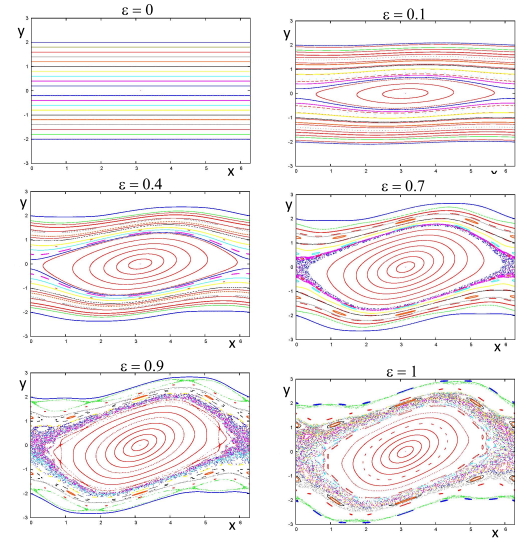
Figure 1: Graphs of the conservative standard map for different values of the perturbing parameter and different initial conditions.

From the upper left plot of Figure 1, we see that for $\varepsilon=0$ the system is integrable; the initial conditions has been chosen to give rotational quasi–periodic curves (lying on straight lines).

When we switch-on the perturbation, even for small values as $\varepsilon=0.1$, the system becomes non–integrable. It is easy to check that there exists a stable equilibrium point at $(\pi,0)$ and an unstable one at $(0,0)$. The quasi–periodic (KAM) curves are distorted with respect to the integrable case and the stable point $(\pi,0)$ is surrounded by elliptic librational islands. The amplitude of the islands increases as $\varepsilon$ gets larger, as it is shown for $\varepsilon=0.4$ where we also notice the appearance of minor resonances. Chaotic dynamics is clearly present for $\varepsilon=0.7$ around the unstable equilibrium point, while the number of rotational quasi–periodic curves decreases when increasing the perturbing parameter. In particular, for $\varepsilon=0.9$ we see large chaotic regions, a few quasi–periodic curves, new islands around higher–order periodic orbits. Finally, for $\varepsilon=1$ we have only chaotic and librational motions, while quasi–periodic curves disappear.

As we will mention in Section 7, there is a wide literature on KAM applications to the standard map to prove the existence of invariant rotational tori with fixed frequency, see [25, 41, 49].

The example we have presented in this Section shows a marked difference with respect to the model that will be presented in Section 2.2, thus witnessing the divergence of the dynamical behaviour between conservative and dissipative dynamical systems. This difference is clearly demonstrated by the dynamics associated to the conservative and dissipative standard maps, as well as by that of more complex systems, like the conservative and dissipative spin-orbit problems, which will be described in Section 2.3.

2.2 The dissipative standard map

The dissipative standard map is obtained from (2.1) adding two parameters: a dissipative parameter $0<\lambda<1$ and a drift parameter $\mu$. For $(y,x)\in\mathbb{R}\times\mathbb{T}$, the equations describing the dissipative standard map are the following:

$$y^{\prime} = \lambda y+\mu+\varepsilon\ V(x)$$

$$x^{\prime} = x+y^{\prime}\ ,$$ (3)

where $\lambda,\varepsilon\in\mathbb{R}_{+}$, $\mu\in\mathbb{R}$. We remark that we obtain the conservative standard map when $\lambda=1$ and $\mu=0$. We also remark that the Jacobian of the mapping (2.2) is equal to $\lambda$, which gives a measure of the rate of contraction or expansion of the area of the phase space. There are several results related to the existence of attractors in the dissipative standard map; a partial list of papers is the following: [6, 7, 48, 60, 62, 90, 95, 98, 100]. Rigorous mathematical works on strange attractors for dissipative 2-D maps with twist are [72, 96, 74].

It is also important to stress that for $\varepsilon=0$ the trajectory $\{y\equiv{\mu\over{1-\lambda}}\}\times\mathbb{T}$, or equivalently $\{\omega\equiv{\mu\over{1-\lambda}}\}\times\mathbb{T}$, is invariant. In fact, for $\varepsilon=0$ we have $y^{\prime}=\lambda y+\mu$ and since we are looking for an invariant object, we need to have $y^{\prime}=y$. Hence, we must solve the equation

$$y=\lambda y+\mu\ .$$ (4)

On the other hand, the frequency $\omega$ associated to the standard map is, by definition, given by

$$\omega=\lim_{j\to\infty}{x_{j}\over j}\ ,$$

which gives $\omega=y$. Combining this last results with (4), we obtain

$$\omega={\mu\over{1-\lambda}}\ ,$$

which shows the strong relation between the frequency and the drift, which cannot be chosen independently. In particular, if we fix the frequency (as it will be required in the KAM theorem of Section 4.2), then we need to tune properly the drift parameter $\mu$. This is a substantial difference with respect to the conservative case; dissipative dynamical systems will require a procedure to prove KAM theory different than in the conservative case.

The dynamics associated to the dissipative standard map admits (see Figure 2) attracting periodic orbits, invariant curve attractors; for different parameters and initial conditions, there appear also strange attractors which have an intricate geometrical structure ([73, 96]): introducing a suitable definition of dimension, the strange attractors are shown to have, for some parameter values, a non–integer dimension (namely a fractal dimension). We will not consider these cases and concentrate in the cases when the attractor is a one-dimensional smooth torus and the motion is smoothly conjugate to a rotation.

We remark that, due to the dissipative character of the map, there might exist at most one invariant curve attractor, while there might be more coexisting periodic orbits (see Figure 2, panel c) and [48]) or strange attractors.

The existence and breakdown of smooth invariant tori in the dissipative standard map have been recently studied in [21] (see also [16]).

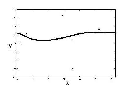
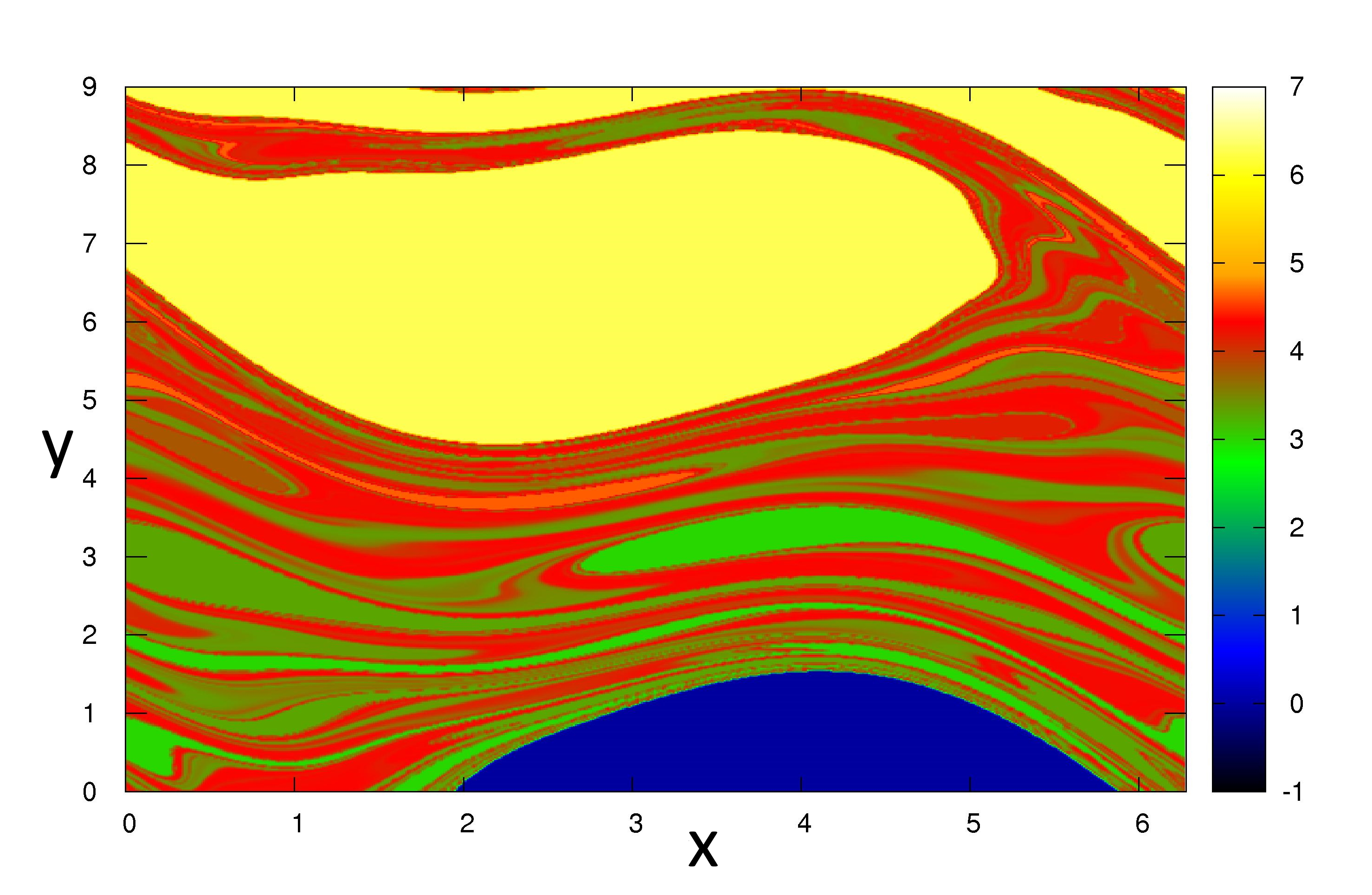
Figure 2: Left: Attractors for the dissipative standard map with $\varepsilon=0.9$, $\lambda=0.91$, $\mu=2\pi(1-\lambda)({{\sqrt{5}-1}\over 2})$. Right: The corresponding basins of attraction using a color scale providing the frequency.

Each of the attractors of Figure 2 is characterized by an associated basin of attraction, which is composed by the set of initial conditions $(x_{0},y_{0})$ whose evolution ends on the given attractor. Figure 2, right, shows the basins of attraction for the case in Figure 2, left; they have been obtained taking $500\times 500$ random initial conditions and looking at their evolution after having performed a number of preliminary iterations.

We want to stress that the role of the drift parameter $\mu$ is of paramount importance in dissipative systems, since an inappropriate choice might prevent to find a specific attractor. An example is given in Figure 3, where we look for the torus with frequency equal to the golden ratio multiplied by the factor $2\pi$, namely $\omega=2\pi\,{{\sqrt{5}-1}\over 2}\simeq 3.8832$, for the dissipative standard map with $\varepsilon=0.1$, $\lambda=0.9$. The upper left panel shows that taking $\mu=0$, the solution spirals on the point attractor at $(\pi,0)$; taking $\mu=0.1$ (Figure 3, upper right panel) leads to an attractor which has frequency different than $\omega$, while the right choice corresponds to $\mu=0.0617984$ as in the left bottom panel of Figure 3. We present in Figure 3, bottom right panel, the behaviour of the drift as a function of the dissipative parameter $\lambda$, which shows that $\mu$ tends to zero in the limit of the conservative case, as it is expected.

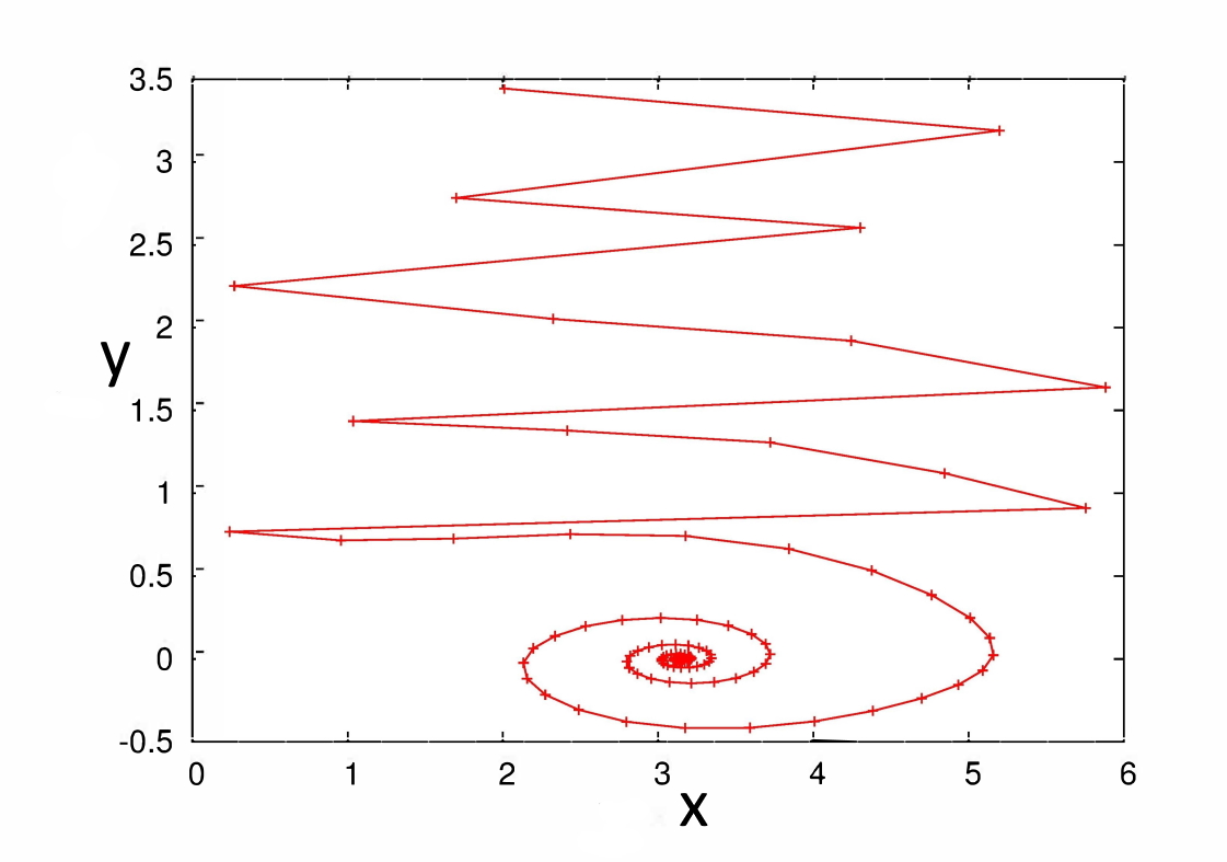
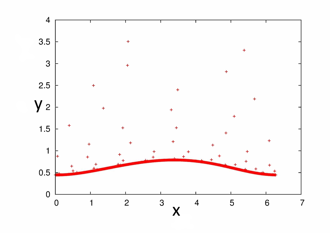
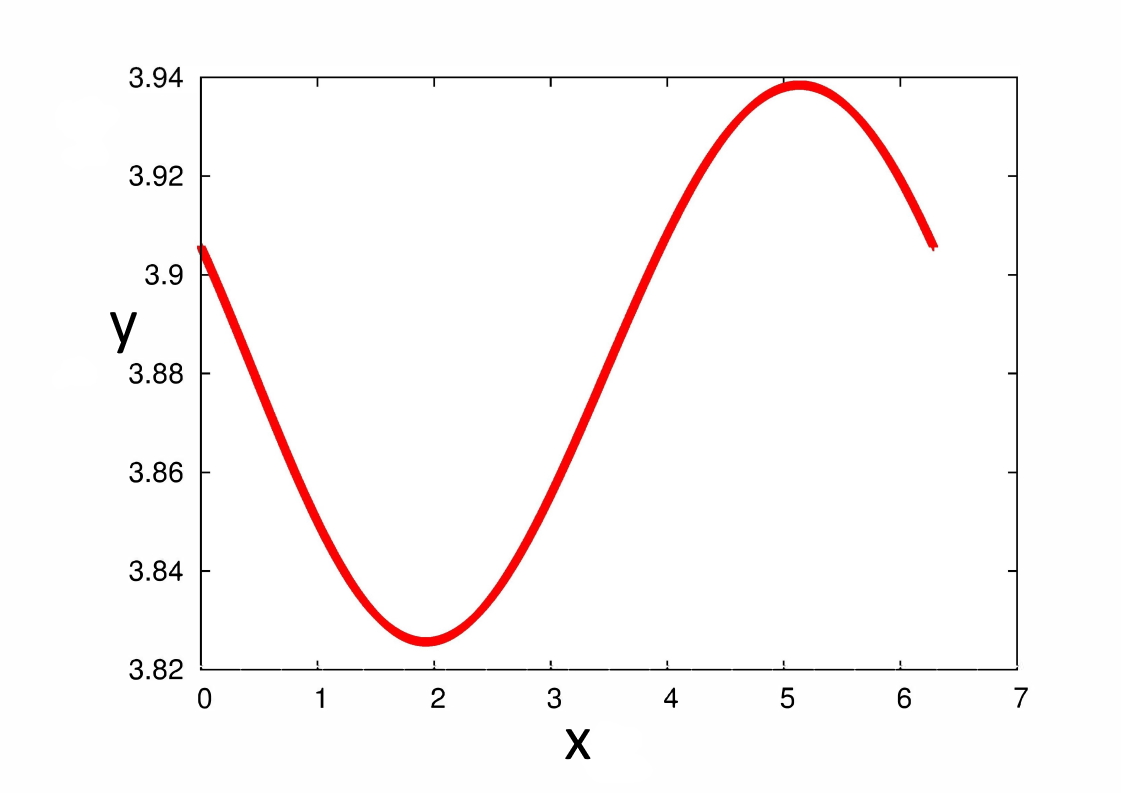
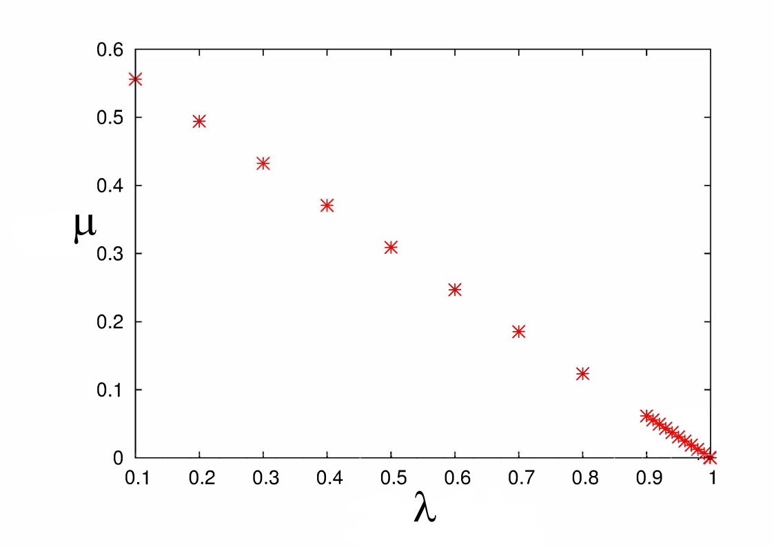
Figure 3: The dissipative standard map for different values of the drift: $\mu=0$ upper left, $\mu=0.1$ upper right, $\mu=0.0617984$ bottom left. Graph of $\mu$ vs. $\lambda$, bottom right.

The twist condition for the dissipative standard map is a condition that now involves the parameters. A non-twist version of the dissipative standard map is the following map,

$$y^{\prime} = \lambda y+\varepsilon\ V(x)$$

$$x^{\prime} = x+(y^{\prime}-a)^{2}+\mu\ .$$ (5)

In figure 4, we notice that this map has parameter values where the rotation number does not change in a monotone direction when we change parameter $a$. See [13] for a study of the invariant circles of the map (2.2).

Figure 4: Rotation number $\rho$ in the map (2.2) w.r.t. the parameter $a$. Reproduced from [13].

2.3 The spin-orbit problems

An interesting example of a continuous system which shows the main dynamical features of regular and chaotic invariant objects is the so-called spin-orbit problem in Celestial Mechanics. The conservative version of the model is based upon the following assumptions. We consider a triaxial satellite, say $\cal S$, with principal moments of inertia $I_{1}<I_{2}<I_{3}$. We assume that the satellite moves on a Keplerian orbit around a central planet, say $\cal P$, while it rotates around a spin–axis perpendicular to the orbit plane and coinciding with its shortest physical axis.

We take a reference system centered in the planet and with the horizontal axis coinciding with the direction of the semimajor axis. We denote by $r$ the orbital radius, by $f$ the true anomaly, while we denote by $x$ the angle between the semimajor axis and the direction of the longest axis of the ellipsoidal satellite (see Figure 5).

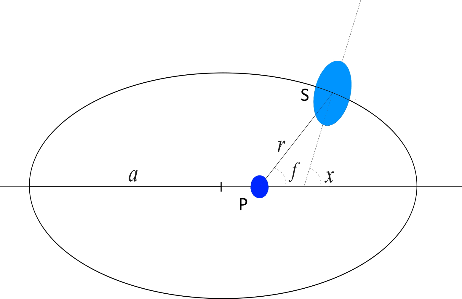
Figure 5: The spin-orbit problem.

The equation of motion describing the conservative spin-orbit problem is

$$\ddot{x}\ +\varepsilon\ \left({a\over r}\right)^{3}\sin(2x-2f)=0\ ,$$ (6)

where $\varepsilon={3\over 2}{{I_{2}-I_{1}}\over I_{3}}$ is a parameter which measures the equatorial flattening of the satellite. Equation (6) is associated to the one-dimensional, time-dependent Hamiltonian function:

$${\cal H}(y,x,t)={y^{2}\over 2}-{\varepsilon\over 2}\Big{(}{a\over r(t)}\Big{)}^{3}\cos(2x-2f(t))\ .$$ (7)

Due to the assumptions of the model, the quantities $r$ and $f$ are known functions of the time, being the solution of Kepler’s problem which determines the elliptical orbit of the satellite. They depend on the orbital eccentricity, which plays the role of an additional parameter.

It is important to observe that:

- the Hamiltonian (7) is integrable whenever $\varepsilon=0$, namely the satellite has equatorial symmetry with $I_{1}=I_{2}$;

- the Hamiltonian (7) is integrable when the eccentricity is equal to zero, since the orbit becomes circular, namely $r=a$ and $f$ coincides with the mean anomaly, which is proportional to time.

The existence and breakdown of invariant tori in the conservative spin-orbit problem have been investigated in [30, 29].

We remark that Hamilton’s equations associated to (7) are given by

$$\dot{x} = y$$

$$\dot{y} = -\varepsilon\Big{(}{a\over r(t)}\Big{)}^{3}\sin(2x-2f(t))\ .$$ (8)

Integrating (2.3) with a modified Euler’s method with time-step $h$, we obtain a discrete system which retains the many features of the conservative standard map when taking the solution on the Poincaré map at time intervals multiple of $2\pi$:

$$y_{n+1} = y_{n}-\varepsilon\Big{(}{a\over r(t_{n})}\Big{)}^{3}\sin(2x_{n}-2f(t_{n}))\ h$$

$$x_{n+1} = x_{n}+y_{n+1}\ h$$

$$t_{n+1} = t_{n}+h\ .$$

The dissipative spin-orbit problem is obtained by taking into account that the satellite is non rigid and therefore it is subject to a tidal torque. The equation of motion including a model for the tidal torque can be written as

$$\ddot{x}\ +\varepsilon\ \left({a\over r}\right)^{3}\sin(2x-2f)=-K_{d}\ [L(e,t)\dot{x}-N(e,t)]\ ,$$ (9)

where

$$L(e,t)={a^{6}\over r^{6}}\ ,\qquad N(e,t)={a^{6}\over r^{6}}\ \dot{f}\$$

(see, e.g., [31, 80]). The coefficient $K_{d}$ is called the dissipative constant, and depends on the physical and orbital features of the body:

$$K_{d}=3n{k_{2}\over{\xi Q}}\left({R_{e}\over a}\right)^{3}{M\over m}\ ,$$

where $n$ is the mean motion, $k_{2}$ is the so-called Love number (depending on the structure of the satellite), $Q$ is called the quality factor (it compares the frequency of oscillation of the system to the rate of dissipation of the energy), $\xi$ is a structure constant such that $I_{3}=\xi mR_{e}^{2}$ with $R_{e}$ the equatorial radius, $M$ is the mass of the planet, $m$ is the mass of the satellite. For bodies like the Moon or Mercury, realistic values are $\varepsilon=10^{-4}$ and $K_{d}=10^{-8}$.

The expression for the tidal torque can be simplified by assuming (as, e.g., in [37]) that the dynamics is ruled by the averages of $L(e,t)$ and $N(e,t)$ over one orbital period. The averaged quantities are given by

$${\overline{L}}(e) = {1\over{(1-e^{2})^{9\over 2}}}\ \left(1+3e^{2}+{3\over 8}e^{4}\right)\ ,$$

$${\overline{N}}(e) = {1\over{(1-e^{2})^{6}}}\ \left(1+{{15}\over 2}e^{2}+{{45}\over 8}e^{4}+{5\over{16}}e^{6}\right)\ .$$

Hence, we obtain the following equation of motion in the averaged case:

$$\ddot{x}+\varepsilon\ \Big{(}{a\over r}\Big{)}^{3}\sin(2x-2f)=-K_{d}\ \Big{(}{\overline{L}}(e)\dot{x}-{\overline{N}}(e)\Big{)}\ ,$$ (10)

We can refer to the quantity $\lambda=K_{d}{\overline{L}}(e)$ as the dissipative parameter and to $\mu={{{\overline{N}}(e)}\over{{\overline{L}}(e)}}$ as the drift parameter.

Let us write (10) in normal form as

$$\dot{x} = y$$

$$\dot{y} = -\varepsilon\Big{(}{a\over r(t)}\Big{)}^{3}\sin(2x-2f(t))-\lambda(y-\mu)\ .$$ (11)

Similarly to the conservative case, the integration of (2.3) with a modified Euler’s method with time-step $h$, leads to a discrete system similar to the dissipative standard map with dissipative and drift parameters, when taking the solution on the Poincaré map at time intervals multiple of $2\pi$:

$$y_{n+1} = (1-\lambda h)y_{n}+\lambda\,\mu\,h-\varepsilon\Big{(}{a\over r(t_{n})}\Big{)}^{3}\sin(2x_{n}-2f(t_{n}))\ h$$

$$x_{n+1} = x_{n}+y_{n+1}\ h$$

$$t_{n+1} = t_{n}+h\ .$$

As we will mention in Section 7, the existence and breakdown of invariant attractors in the dissipative spin-orbit problem have been studied in [24] through an application of KAM theory for conformally symplectic systems and through suitable numerical methods.

3 Conformally symplectic systems and Diophantine vectors

In this section we give the definition of conformally symplectic systems for maps and flows (see Section 3.1) and we introduce the set of Diophantine vectors for discrete and continuous systems (see Section 3.2).

3.1 Discrete and continuous conformally symplectic systems

An important class of dissipative dynamical systems is given by the conformally symplectic systems; the dissipative standard map is an example of a conformally symplectic discrete system, while the dissipative spin-orbit problem is an example of a conformally symplectic continuous system.

Before giving the formal definition, let us say that conformally symplectic systems are characterized by the property that they transform the symplectic form into a multiple of itself. Beside the examples mentioned before, we stress that conformally symplectic models can be found in different fields, e.g. the Euler-Lagrange equations of exponentially discounted systems ([5], typically found in finance, when inflation is present and one needs to minimize the cost in present money) or Gaussian thermostats ([46, 99], namely mechanical systems with forcing and a thermostating term based on the Gauss Least Constraint Principle for nonholonomic constraints).

Let us start to introduce the notion of $2n$-dimensional conformally symplectic maps. Let ${\cal M}=U\times\mathbb{T}^{n}$ be the phase space with $U\subseteq\mathbb{R}^{n}$ an open, simply connected domain with smooth boundary; the phase space ${\cal M}$ is endowed with the standard scalar product and a symplectic form $\Omega$, represented by a matrix $J$ at the point ${\underline{z}}$ acting on vectors ${\underline{u}},{\underline{v}}\in\mathbb{R}^{n}$ as $\Omega({\underline{u}},{\underline{v}})=({\underline{u}},J({\underline{z}}){\underline{v}})$ with $(\cdot,\cdot)$ denoting the scalar product. Note that the matrix $J$ depends not only on the symplectic form but on the metric considered.

Definition 3.1.

A diffeomorphism $f$ on $\cal M$ is conformally symplectic, if there exists a function $\lambda:{\cal M}\to\mathbb{R}$ such that, denoting by $f^{*}$ the pull–back of $f$, we have:

$$f^{*}\Omega=\lambda\Omega\ .$$ (12)

We remark that for $n=1$ any diffeomorphism is conformally symplectic with $\lambda$ depending on the coordinates, namely one can take $\lambda(x)=det(Df(x))$ or $\lambda(x)=-det(Df(x))$. Instead, for $n\geq 2$ one obtains that $\lambda$ is a constant. In fact, taking the exterior derivative of $f^{*}\Omega=\lambda\Omega$, one obtains:

$$d(f^{*}\Omega)=f^{*}\ d\Omega=0\ =\ d\lambda\wedge\Omega+\lambda\wedge d\Omega=d\lambda\wedge\Omega\ ,$$

which gives $d\lambda=0$; since the manifold is simply connected, then $\lambda$ is equal to a constant (see [17]).

We also remark that for $\lambda=1$ (and $\mu=0$) we recover the symplectic case.

Let us give some explicit examples which might help to clarify the meaning of Definition 3.1. First, we notice that we can re-formulate the notion of conformally symplectic by saying that the diffeomorphism $f$ is conformally symplectic if

$$Df^{T}\,J\,Df=\lambda\ J\ ,$$ (13)

where the superscript $T$ denotes transposition. In fact, from (12) we have:

$$f^{\ast}\Omega=\lambda\Omega \Leftrightarrow \Omega(Df\ {\underline{u}},Df\ {\underline{v}})=\lambda\ \Omega({\underline{u}},{\underline{v}})$$

$$\Leftrightarrow (Df\ {\underline{u}},J\,Df\ {\underline{v}})=\lambda\ ({\underline{u}},J\ {\underline{v}})$$

$$\Leftrightarrow (u,Df^{T}\,J\,Df\,{\underline{v}})=({\underline{u}},\lambda\,J\ {\underline{v}})$$

$$\Leftrightarrow Df^{T}\,J\,Df=\lambda\ J\ .$$

An example of a conformally symplectic diffeomorphism is given by the dissipative standard map. Recalling (2.2), we have that (13) is satisfied, as shown below:

$$\left(\begin{array}[]{cc}\lambda&\lambda\\ \varepsilon V_{x}&1+\varepsilon V_{x}\\ \end{array}\right)\ \left(\begin{array}[]{cc}0&1\\ -1&0\\ \end{array}\right)\ \left(\begin{array}[]{cc}\lambda&\varepsilon V_{x}\\ \lambda&1+\varepsilon V_{x}\\ \end{array}\right)=\left(\begin{array}[]{cc}0&\lambda\\ -\lambda&0\\ \end{array}\right)\ \ =\lambda\,J\ .$$

An example of a map which does not satisfy the conformally symplectic condition (13) is given by the following 4-dimensional dissipative standard map with conformal factors $\lambda_{1}$, $\lambda_{2}$ with $\lambda_{1}\not=\lambda_{2}$:

$$y_{1}^{\prime} = \lambda_{1}y_{1}+\mu_{1}+\varepsilon V_{1}(x_{1},x_{2})$$

$$y_{2}^{\prime} = \lambda_{2}y_{2}+\mu_{2}+\varepsilon V_{2}(x_{1},x_{2})$$

$$x_{1}^{\prime} = x_{1}+y_{1}^{\prime}$$

$$x_{2}^{\prime} = x_{2}+y_{2}^{\prime}\ .$$

In fact, even for $\varepsilon=0$, we obtain that (13) is not satisfied:

$$Df^{T}\,J\,Df=\left(\begin{array}[]{cccc}0&0&\lambda_{1}&0\\ 0&0&0&\lambda_{2}\\ -\lambda_{1}&0&0&0\\ 0&-\lambda_{2}&0&0\\ \end{array}\right)\not=\lambda\ \left(\begin{array}[]{cccc}0&0&1&0\\ 0&0&0&1\\ -1&0&0&0\\ 0&-1&0&0\\ \end{array}\right)=\lambda\ J\ .$$

To conclude, we give the definition of conformally symplectic systems for continuous dynamical systems.

Definition 3.2.

We say that a vector field $X$ is a conformally symplectic flow if, denoting by $L_{X}$ the Lie derivative, there exists a function $\lambda:\mathbb{R}^{2n}\to\mathbb{R}$ such that

$$L_{X}\Omega=\lambda\Omega\ .$$

In analogy to the definition of conformally symplectic maps, we remark that the time $t$-flow $\Phi_{t}$ satisfies the relation

$$(\Phi_{t})^{*}\Omega=e^{\lambda t}\Omega\ .$$

3.2 Diophantine vectors for maps and flows

In this Section we give the definition of Diophantine vectors for maps and flows and we briefly recall the main properties of Diophantine vectors. We start by giving the definition for maps.

Definition 3.3.

We say that the vector $\omega\in\mathbb{R}^{n}$ satisfies the Diophantine condition, if for a constant $C>0$ and an exponent $\tau>0$, one has

$$\left|{{{\underline{\omega}}\cdot{\underline{q}}}\over{2\pi}}-p\right|^{-1}\ \leq\ C|q|^{\tau}\ ,\qquad p\in\mathbb{Z}\ ,\quad q\in\mathbb{Z}^{n}\backslash\{0\}\ .$$

In the case of flows we have the following definition.

Definition 3.4.

We say that the vector $\omega\in\mathbb{R}^{n}$ satisfies the Diophantine condition, if for a Diophantine constant $C>0$ and a Diophantine exponent $\tau>0$, one has:

$$|{\underline{\omega}}\cdot{\underline{k}}|^{-1}\ \leq\ C|{\underline{k}}|^{\tau}\ ,\qquad{\underline{k}}\in\mathbb{Z}^{n}\backslash\{0\}\ .$$

We conclude this Section by listing below some important properties of Diophantine vectors.

$(i)$ Let us denote by $\mathcal{D}(C,\tau)$ the set of Diophantine vectors satisfying Definition 3.4. Then, the size of the set of Diophantine vectors $\mathcal{D}(C,\tau)$ increases as $C$ or $\tau$ increases. The set of vectors that satisfy this condition for some $C,\tau$. is of full Lebesgue measure in $\mathbb{R}^{n}$.

$(ii)$ There are no Diophantine vectors in $\mathbb{R}^{n}$ with $\tau<n-1$.

$(iii)$ The set of Diophantine vectors with $\tau=n-1$ in $\mathbb{R}^{n}$ has zero Lebesgue measure, but it is everywhere dense.

$(iv)$ For $\tau>n-1$, almost every vector in $\mathbb{R}^{n}$ is $\tau$-Diophantine, namely the complement has zero Lebesgue measure, although it is everywhere dense.

4 Invariant tori and KAM theory for conformally symplectic systems

In this Section we provide the definition of KAM (rotational) invariant tori (for maps and flows) (see Section 4.1); the statement of the KAM theorem for conformally symplectic maps is given in Section 4.2, whose proof is briefly recalled in Section 4.3. The proof can be translated into a very efficient KAM algorithm (see [17]), which is at the basis of different results: the derivation of numerical methods to compute the breakdown threshold (Section 5), the investigation of the breakdown mechanism (Section 6), the implementations to specific models (see Section 7).

4.1 Invariant KAM tori

We start by giving the definition of conditionally periodic and quasi-periodic motions.

Definition 4.1.

A conditionally periodic motion is represented by a function $t\mapsto f(\omega_{1}t,\ldots,\omega_{n}t)$, where $f(x_{1},\ldots,x_{n})$ is periodic in all variables; the vector ${\underline{\omega}}=(\omega_{1},\ldots,\omega_{n})$ is called frequency.

A quasi-periodic motion is a conditionally periodic motion with incommensurable frequencies.

Next we give the following definition of invariant torus.

Definition 4.2.

An invariant torus is an invariant manifold diffeomorphic to the standard torus $\mathbb{T}^{n}$.

We remark that any trajectory on an invariant torus carrying quasi-periodic motions is dense on the torus. We conclude by giving the definition of (rotational) KAM torus for maps and flows. This definition is based on the invariance equation (14) below, whose solution will be the centerpiece of the KAM theorem presented in Section 4.2.

Definition 4.3.

Let ${\cal M}\subseteq\mathbb{R}^{n}\times\mathbb{T}^{n}$ be a symplectic manifold and let $f:{\cal M}\rightarrow{\cal M}$ be a symplectic map. A KAM torus with frequency ${\underline{\omega}}\in\mathcal{D}(C,\tau)$ is an $n$–dimensional invariant torus described parametrically by an embedding $K:\mathbb{T}^{n}\rightarrow{\cal M}$, which is the solutions of the invariance equation:

$$f\circ K({\underline{\theta}})=K({\underline{\theta}}+{\underline{\omega}})\ .$$ (14)

For a family $f_{\mu}$ of conformally symplectic diffeomorphisms depending on a real parameter $\mu$, a KAM attractor with frequency ${\underline{\omega}}\in\mathcal{D}(C,\tau)$ is an $n$–dimensional invariant torus described parametrically by an embedding $K:\mathbb{T}^{n}\rightarrow{\cal M}$ and a drift $\mu$, which are the solutions of the invariance equation:

$$f_{\mu}\circ K({\underline{\theta}})=K({\underline{\theta}}+{\underline{\omega}})\ .$$ (15)

For conformally symplectic vector fields $X_{\mu}$, the invariance equation is given by

$$X_{\mu}\circ K({\underline{\theta}})=({\underline{\omega}}\cdot\partial_{\underline{\theta}})\ K({\underline{\theta}})\ .$$

We remark that for symplectic systems the invariance equation (14) contains as only unknown the embedding $K$, while for conformally symplectic systems the invariance equation (15) contains as unknowns both the embedding $K$ and the drift term $\mu$.

A graphical representation of the invariance equation (14) is given in Figure 6.

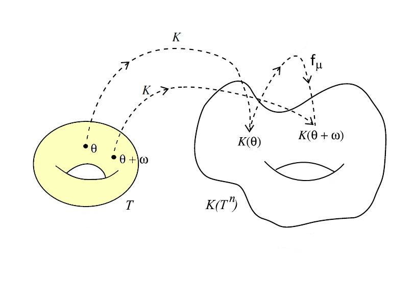
Figure 6: Geometric interpretation of the invariance equation $f_{\mu}\circ K({\underline{\theta}})=K({\underline{\theta}}+{\underline{\omega}})$ in the unknowns $K$, $\mu$.

Although the theory that will be presented in the next Sections apply both to maps and flows, for simplicity of exposition we will limit to the presentation of KAM theory for maps. We refer to [17] for the details concerning continuous systems.

4.2 Conformally symplectic KAM theorem

We will try to answer a specific question, which is formulated below, by means of a suitable statement of the KAM theorem; the question is motivated by many applications in several models of Celestial Mechanics, which are often described by nearly-integrable systems. This is why we set the following question in the framework of nearly-integrable systems, although the formulation of KAM theory does not need that the system is close to integrable (compare with [39]).

Assume that a given integrable dynamical system admits an invariant torus run by a quasi-periodic motion with frequency $\underline{\omega}$ (e.g., think at Kepler’s 2-body problem). Consider a perturbation of the integrable system (e.g., the restricted 3-body problem, which is described by the 2-body problem with a perturbation proportional to the primaries’ mass ratio). The main question that we want to raise in the framework of KAM theory for nearly-integrable systems is the following: does the perturbed system still admits an invariant torus run by a quasi-periodic motion with the same frequency as the unperturbed system? The answer is given by celebrated KAM theory ([68, 1, 78]), which can be implemented under very general assumptions, precisely a non-degeneracy condition of the unperturbed system and a Diophantine condition on the frequency.

We remark that invariant tori are Lagrangian: if $f$ is a symplectic map and $K$ satisfies the invariance equation (14), then

$$K^{*}\Omega=0\ .$$ (16)

The same holds for a conformally symplectic map $f_{\mu}$, when $|\lambda|\neq 1$ and $K$ satisfies the invariance equation (15). If $f$ is symplectic and $\underline{\omega}$ is irrational, then the torus is Lagrangian, i.e. with maximal dimension and isotropic (namely, the symplectic form restricted on the manifold is zero, which implies that each tangent space is an isotropic subspace of the ambient manifold’s tangent space).

Next step is to consider a nearly-integrable dynamical system affected by a dissipative force, so that the overall system is conformally symplectic (an example is given by the spin-orbit problem with tidal torque). We assume that the integrable symplectic system admits an invariant torus with Diophantine frequency; the question becomes whether the non-integrable system with dissipation still admits, for suitable values of the drift parameter, an invariant attractor run by a quasi-periodic motion with the same frequency of the unperturbed system. The answer is given by the KAM theorem for conformally symplectic systems as given by Theorem 4.5 (see [17]).

Since we will be interested to give explicit estimates in specific model problems, we introduce the following norms for analytic and differentiable functions.

Definition 4.4.

Analytic norm. Given $\rho>0$, we define the complex extension of the torus, say $\mathbb{T}_{\rho}^{n}$, as the set

$$\mathbb{T}_{\rho}^{n}=\{{\underline{\theta}}\in\mathbb{C}^{n}/(2\pi\mathbb{Z})^{n}:\ {\rm Re}({\underline{\theta}})\in\mathbb{T}^{n},\ |{\rm Im}(\theta_{j})|\leq\rho\ ,\ \ j=1,...,n\}\ ;$$

we denote by ${\cal A}_{\rho}$ the set of analytic functions in $Int(\mathbb{T}_{\rho}^{n})$ with the norm

$$\|f\|_{\rho}=\sup_{{\underline{\theta}}\in\mathbb{T}_{\rho}^{n}}\ |f({\underline{\theta}})|\ .$$

Sobolev norm. For a function $f=f({\underline{z}})$ expanded in Fourier series as $f({\underline{z}})=\sum_{{\underline{k}}\in{\mathbb{Z}}^{n}}\widehat{f_{\underline{k}}}\ e^{2\pi i{\underline{k}}\cdot{\underline{z}}}$ for an integer $m>0$, we define the space $H^{m}$ as

$$H^{m}=\Big{\{}f:\mathbb{T}^{n}\to\mathbb{C}\ :\ \|f\|_{m}^{2}\equiv\sum_{{\underline{k}}\in{\mathbb{Z}}^{n}}|\,\widehat{f_{\underline{k}}}\,|^{2}(1+|{\underline{k}}|^{2})^{m}<\infty\Big{\}}\ .$$

Borrowing the statement from [17], we give below the formulation of the KAM theorem for conformally symplectic systems (see [39] for the statement for symplectic systems). We give the statement for maps, although the results can be formulated also for systems with continuous time (flows). Indeed in [17] one can find a construction that shows that the results for maps imply the results for flows as well as direct proof of the results for flows.

Theorem 4.5.

Let ${\underline{\omega}}\in\mathcal{D}(C,\tau)$, $f_{\mu}:\mathbb{R}^{n}\times\mathbb{T}^{n}\rightarrow\mathbb{R}^{n}\times\mathbb{T}^{n}$ be a conformally symplectic diffeomorphism, and let $(K,\mu)$ be an approximate solution of the invariance equation (15) with error term $E$:

$$f_{\mu}\circ K({\underline{\theta}})-K({\underline{\theta}}+{\underline{\omega}})=E({\underline{\theta}})\ .$$

Let $N$ be the quantity

$$N({\underline{\theta}})=(DK({\underline{\theta}})^{T}DK({\underline{\theta}}))^{-1}$$ (17)

and let $M({\underline{\theta}})$ be the $2n\times 2n$ matrix defined by

$$M({\underline{\theta}})=[DK({\underline{\theta}})\ |\ J(K({\underline{\theta}}))^{-1}\ DK({\underline{\theta}})N({\underline{\theta}})]\ .$$

Let $P({\underline{\theta}})$ be defined as

$$P(\theta)\equiv DK(\theta)N(\theta)\ ;$$

let $A(\theta)\equiv\lambda\,\rm Id$ and let $S({\underline{\theta}})$ be

$$S(\theta)\equiv P(\theta+\omega)^{T}Df_{\mu}\circ K(\theta)J^{-1}\circ K(\theta)P(\theta)-N(\theta+\omega)^{T}\gamma(\theta+\omega)N(\theta+\omega)A(\theta)$$ (18)

with

$$\gamma(\theta)\equiv DK(\theta)^{T}J^{-1}\circ K(\theta)DK(\theta)\ .$$

Assume that the following non–degeneracy condition is satisfied:

$$\det\left(\begin{array}[]{cc}\langle S\rangle&{\langle{SB^{0}}}\rangle+\langle{\widetilde{A}_{1}}\rangle\\ (\lambda-1){\rm Id}&\langle{\widetilde{A}_{2}}\rangle\\ \end{array}\right)\neq 0$$ (19)

with $\widetilde{A}_{1}$, $\widetilde{A}_{2}$ the first and second $n$ columns of $\tilde{A}=M^{-1}({\underline{\theta}}+{\underline{\omega}})D_{\mu}f_{\mu}\circ K$, $B^{0}=B-\langle B\rangle$ is the solution of $\lambda B^{0}({\underline{\theta}})-B^{0}({\underline{\theta}}+{\underline{\omega}})=-(\widetilde{A}_{2})^{0}({\underline{\theta}})$.

For $\rho>0$, let $0<\delta<{\rho\over 2}$; if the solution is sufficiently approximate, namely

$$\|E\|_{\rho}\leq C_{3}\ C^{-4}\ \delta^{4\tau}$$

for a suitable constant $C_{3}>0$, then there exists an exact solution $(K_{e},\mu_{e})$, such that

$$\|K_{e}-K\|_{\rho-2\delta}\leq C_{4}\ C^{2}\ \delta^{-2\tau}\ \|E\|_{\rho}\ ,\quad|\mu_{e}-\mu|\leq C_{5}\ \|E\|_{\rho}$$

with suitable constants $C_{4},C_{5}>0$.

Remark 4.6.

It is useful to make a remark on the non–degeneracy condition (19), when applied to the conservative and dissipative standard maps ((2.1), (2.2)). For the conservative standard map, the non–degeneracy condition is typically the so-called twist condition, which can be written as

$${{\partial x^{\prime}}\over{\partial y}}\not=0\ ,$$ (20)

implying that the lift of the map transforms any vertical line always on the same side.

Instead, for the dissipative standard map, that we modify adding a generic dependence on the drift through a function $p=p(\mu)$, say

$$y^{\prime} = \lambda y+p(\mu)+\varepsilon\ V(x)$$

$$x^{\prime} = x+y^{\prime}\ ,$$

then the non–degeneracy condition involves the twist condition and a non–degeneracy condition with respect to to the parameters, namely:

$${{\partial x^{\prime}}\over{\partial y}}\not=0\ ,\qquad\qquad{{dp(\mu)}\over{d\mu}}\not=0\ .$$ (21)

We remark, however, that (20) and (21) involve global properties of the system, while (19) is a condition involving just the approximate solution, so that (19) may be applied in situations where (19), (21) fail.

The proof of Theorem 4.5 is given in [17] through the a-posteriori approach developed in [39] and making use of an adjustment of parameters (see [79, 8]): assume we can find an approximate solution $(K,\mu)$ of the invariance equation, satisfying a non-degeneracy condition, then we can find a true solution $(K_{e},\mu_{e})$ close to $(K,\mu)$, such that $\|K_{e}-K\|$, $|\mu_{e}-\mu|$ is small. A sketch of the proof of Theorem 4.5 is presented in Section 4.3.

We conclude this Section by remarking that the a-posteriori approach presents several advantages, among which:

• $(i)$ it can be developed in any coordinate frame and not necessarily in action-angle variables. In many practical problems, the action-angle variables are difficult to compute and involve complex singularities.

  Of course, once we have the existence of the torus, we can construct action angle variables. Hence, compared to more standard results, the accomplishment of the method is that the existence of action variables and the quasi-integrablility is moved from the hypothesis to the conclusions. This is useful in practice since the hypothesis is hard to verify in applications.

  Of course, moving conclusions to hypothesis without regards on how to check them, one can get the same conclusions. In that respect, adding the hypothesis of the existence of the torus would get a theorem with the same applicability and a simpler proof.

• $(ii)$ The system is not assumed to be nearly integrable.

• $(iii)$ Instead of constructing a sequence of coordinate transformations on shrinking domains as in the perturbation approach, one computes suitable corrections to the embedding and the drift.

  The computation of the embeddings requires to work only with variables of $n$ dimensions whereas transformation theory requires to work with variables in $2n$ dimensions. The complexity of representing functions grows exponentially – with a large exponent – on the dimension. The composition of two functions has rather awkward analytic and numerical properties.

• $(iv)$ The non-degeneracy assumptions are not global properties of the map, but are rather properties of the approximate solution considered.

• $(v)$ One does not need to justify how the approximate solution was obtained. In particular, one can take as approximate solution the result of numerical calculations or a formal expansion.

  Verifying the hypothesis in a numerical approximation is just a finite number of calculations. Even if this number is too large to do by hand, it could be moderate to do with a computer (e.g., a few hours in a common laptop). If these can be done taking care of roundoff and truncation errors, this may lead to a computer assisted proof.

  One can also verify the hypothesis easily in a numerical expansion.

  Note that, in these verifications it is crucial as noted in $(i)$ to move the difficult to verify facts from the hypothesis that need to be checked to the conclusions.

4.3 A sketch of the proof of the KAM theorem

The proof of Theorem 4.5 can be summarized as composed by five main steps:

• Step 1: starting from an approximate solution, write the linearization of the invariance equation.

• Step 2: by a Newton’s method find a quadratically smaller approximation.

• Step 3: under a non–degeneracy condition, solve the cohomological equation that allows to find the new approximation.

• Step 4: iterate the procedure and show its convergence.

• Step 5: prove that the solution is locally unique.

We briefly describe such steps as follows.

4.3.1 Step 1: approximate solution and linearization.

Let $(K,\mu)$ be an approximate solution satisfying

$$f_{\mu}\circ K({\underline{\theta}})-K({\underline{\theta}}+{\underline{\omega}})=E({\underline{\theta}})\ .$$ (22)

Using the Lagrangian property $K^{*}\Omega=0$ written in coordinates, namely

$$DK^{T}({\underline{\theta}})\ J\circ K({\underline{\theta}})\ DK({\underline{\theta}})=0\ ,$$

we get that the tangent space is given by

$$Range\Big{(}DK({\underline{\theta}})\Big{)}\oplus Range\Big{(}V({\underline{\theta}})\Big{)}$$ (23)

with $N$ as in (17) and

$$V({\underline{\theta}})=J^{-1}\circ K({\underline{\theta}})\ DK({\underline{\theta}})N({\underline{\theta}})\ .$$

Define the quantity

$$M({\underline{\theta}})=[DK({\underline{\theta}})\ |\ V({\underline{\theta}})]\ .$$ (24)

Then, we have the following result.

Lemma 4.7.

Up to a remainder $R$, we have the following relation:

$$Df_{\mu}\circ K({\underline{\theta}})\ M({\underline{\theta}})=M({\underline{\theta}}+{\underline{\omega}})\left(\begin{array}[]{cc}\rm Id&S({\underline{\theta}})\\ 0&\lambda\rm Id\\ \end{array}\right)+R({\underline{\theta}})\ .$$

Proof 4.8.

Recalling the definition of $M$ in (24), we have that taking the derivative of

$$f_{\mu}\circ K({\underline{\theta}})=K({\underline{\theta}}+{\underline{\omega}})+E({\underline{\theta}})\ ,$$

one obtains the relation

$$Df_{\mu}\circ K({\underline{\theta}})\ DK({\underline{\theta}})=DK({\underline{\theta}}+{\underline{\omega}})+DE({\underline{\theta}})\ .$$

Due to (23), one obtains:

$$Df_{\mu}\circ K({\underline{\theta}})\ V({\underline{\theta}})=DK({\underline{\theta}}+{\underline{\omega}})\ S({\underline{\theta}})+V({\underline{\theta}}+{\underline{\omega}})\ \lambda\ {\rm Id}+h.o.t.$$

with $S$ as in (18).

4.3.2 Step 2: determine a new approximation.

Let the new approximation $(K^{\prime},\mu^{\prime})$ be defined as $K^{\prime}=K+MW$, $\mu^{\prime}=\mu+\sigma$. Let $E^{\prime}$ be the error associated to $(K^{\prime},\mu^{\prime})$:

$$f_{\mu^{\prime}}\circ K^{\prime}({\underline{\theta}})-K^{\prime}({\underline{\theta}}+{\underline{\omega}})=E^{\prime}({\underline{\theta}})\ .$$ (25)

Expanding (25) in Taylor series, we get

$$f_{\mu}\circ K({\underline{\theta}})+Df_{\mu}\circ K({\underline{\theta}})\ M({\underline{\theta}})W({\underline{\theta}})+D_{\mu}f_{\mu}\circ K({\underline{\theta}})\sigma$$

$$\qquad-K({\underline{\theta}}+{\underline{\omega}})-M({\underline{\theta}}+{\underline{\omega}})\ W({\underline{\theta}}+{\underline{\omega}})+h.o.t.=E^{\prime}({\underline{\theta}})\ .$$

Recalling (22), the new error $E^{\prime}$ is quadratically smaller provided the following relation holds:

$$Df_{\mu}\circ K({\underline{\theta}})\ M({\underline{\theta}})W({\underline{\theta}})-M({\underline{\theta}}+{\underline{\omega}})\ W({\underline{\theta}}+{\underline{\omega}})+D_{\mu}f_{\mu}\circ K({\underline{\theta}})\sigma=-E({\underline{\theta}})\ .$$ (26)

Combining (26) and Lemma 4.7, we have:

$$Df_{\mu}\circ K({\underline{\theta}})\ M({\underline{\theta}})=M({\underline{\theta}}+{\underline{\omega}})\left(\begin{array}[]{cc}\rm Id&S({\underline{\theta}})\\ 0&\lambda\rm Id\\ \end{array}\right)+R({\underline{\theta}})\ .$$

This allows to get the following equations for $W=(W_{1},W_{2})$ and $\sigma$

$$M({\underline{\theta}}+{\underline{\omega}})\left(\begin{array}[]{cc}\rm Id&S({\underline{\theta}}\\ 0&\lambda\rm Id\\ \end{array}\right)\ W({\underline{\theta}})-M({\underline{\theta}}+{\underline{\omega}})\ W({\underline{\theta}}+{\underline{\omega}})=-E({\underline{\theta}})-D_{\mu}f_{\mu}\circ K({\underline{\theta}})\sigma$$

that we are going to make more explicit. Multiplying by $M({\underline{\theta}}+{\underline{\omega}})^{-1}$ and writing $W=(W_{1},W_{2})$, one gets that the previous equation is equivalent to:

$$\left(\begin{array}[]{cc}\rm Id&S({\underline{\theta}})\\ 0&\lambda\rm Id\\ \end{array}\right)\left(\begin{array}[]{c}W_{1}({\underline{\theta}})\\ W_{2}({\underline{\theta}})\\ \end{array}\right)-\left(\begin{array}[]{c}W_{1}({\underline{\theta}}+{\underline{\omega}})\\ W_{2}({\underline{\theta}}+{\underline{\omega}})\\ \end{array}\right)=\left(\begin{array}[]{c}-\tilde{E}_{1}({\underline{\theta}})-\tilde{A}_{1}({\underline{\theta}})\sigma\\ -\tilde{E}_{2}({\underline{\theta}})-\tilde{A}_{2}({\underline{\theta}})\sigma\\ \end{array}\right)$$ (27)

with $\tilde{E}_{j}({\underline{\theta}})=-(M({\underline{\theta}}+{\underline{\omega}})^{-1}E)_{j}$, $\tilde{A}_{j}({\underline{\theta}})=(M({\underline{\theta}}+{\underline{\omega}})^{-1}D_{\mu}f_{\mu}\circ K)_{j}$. Writing (27) in components, we obtain:

$$W_{1}({\underline{\theta}})-W_{1}({\underline{\theta}}+{\underline{\omega}}) = -\widetilde{E}_{1}({\underline{\theta}})-S({\underline{\theta}})W_{2}({\underline{\theta}})-\widetilde{A}_{1}({\underline{\theta}})\,\sigma$$

$$\lambda W_{2}({\underline{\theta}})-W_{2}({\underline{\theta}}+{\underline{\omega}}) = -\widetilde{E}_{2}({\underline{\theta}})-\widetilde{A}_{2}({\underline{\theta}})\,\sigma\ .$$ (28)

The cohomological equations (4.3.2) allow to find the corrections $W_{1}$, $W_{2}$ and $\sigma$, as sketched in the next step.

4.3.3 Step 3: solve the cohomological equations.

To determine the new approximation, we need to solve equations (4.3.2), which are equations with constant coefficients for $W_{1}$, $W_{2}$ and $\sigma$ for known $S$, $\widetilde{E}\equiv(\widetilde{E}_{1},\widetilde{E}_{2})$, $\widetilde{A}\equiv[\widetilde{A}_{1}|\ \widetilde{A}_{2}]$.

The first equation in (4.3.2) is a standard small divisor equation, which can be solved under the Diophantine condition on the frequency, so to bound the small divisors.

For $|\lambda|\neq 1$ and for all real vectors ${\underline{\omega}}$, it is possible to solve the second equation in (4.3.2) by an elementary contraction mapping argument.

We remark that, using Cauchy estimates for the cohomological equations (4.3.2), we can bound $\|W_{1}\|_{\rho-\delta}$ and $\|W_{2}\|_{\rho-\delta}$ by $\|E\|_{\rho}$.

To solve the cohomological equations, we proceed as follows. Take the averages of each equation in (4.3.2) and use the non–degeneracy condition to determine $\langle W_{2}\rangle$, $\sigma$ by solving the equation

$$\left(\begin{array}[]{cc}\langle S\rangle&{\langle{SB^{0}}}\rangle+\langle{\widetilde{A}_{1}}\rangle\\ (\lambda-1){\rm Id}&\langle{\widetilde{A}_{2}}\rangle\\ \end{array}\right)\left(\begin{array}[]{cc}\langle W_{2}\rangle\\ \sigma\\ \end{array}\right)=\left(\begin{array}[]{cc}-\langle S\tilde{B}^{0}\rangle-\langle\widetilde{E}_{1}\rangle\\ -\langle\widetilde{E_{2}}\rangle\\ \end{array}\right)\ ,$$

where we have split $W_{2}$ as $W_{2}=\langle W_{2}\rangle+B^{0}+\sigma\tilde{B}^{0}$.

Next, we need to solve the second equation in (4.3.2) for $W_{2}$, which is an equation of the form $\lambda W_{2}({\underline{\theta}})-W_{2}({\underline{\theta}}+{\underline{\omega}})=Q_{2}({\underline{\theta}})$ with $Q_{2}$ known. Such equation is always solvable for any $|\lambda|\not=1$ by a contraction mapping argument, using that $\lambda W_{2}({\underline{\theta}})-W_{2}({\underline{\theta}}+{\underline{\omega}})=\sum_{\underline{k}}\widehat{W}_{2,{\underline{k}}}\,e^{i{\underline{k}}\cdot{\underline{\theta}}}(\lambda-e^{i{\underline{k}}\cdot{\underline{\omega}}})$.

Finally, we solve the first equation in (4.3.2) for $W_{1}$, which amounts to solve an equation of the form $W_{1}({\underline{\theta}})-W_{1}({\underline{\theta}}+{\underline{\omega}})=Q_{1}({\underline{\theta}})$ with $Q_{1}$ known. It involves small (zero) divisors, since for ${\underline{k}}={\underline{0}}$ one has $1-e^{i{\underline{k}}\cdot{\underline{\omega}}}=0$. The left hand side of the first equation in (4.3.2) can be expanded as

$$W_{1}({\underline{\theta}})-W_{1}({\underline{\theta}}+{\underline{\omega}})=\sum_{{\underline{k}}\in\mathbb{Z}^{n}\backslash\{{\underline{0}}\}}\widehat{W}_{1,{\underline{k}}}\,e^{i{\underline{k}}\cdot{\underline{\theta}}}(1-e^{i{\underline{k}}\cdot{\underline{\omega}}})\ .$$

To get a bound for the solution of (4.3.2), we need the following result.

Proposition 4.9.

Let $Z=Z({\underline{\theta}})$ be a function with zero average and such that $Z\in{\cal A}_{\rho}$ or $Z\in H^{m}$. Let ${\underline{\omega}}\in D(C,\tau)$. Assume that the function $U=U({\underline{\theta}})$ satisfies

$$\lambda U({\underline{\theta}})-U({\underline{\theta}}+{\underline{\omega}})=Z({\underline{\theta}})\ .$$

Then, if $\lambda\not=1$, $|\lambda|\in[A,A^{-1}]$ for $0<A<1$, we have that

$$\|U({\underline{\theta}})\|_{\rho-\delta}\leq C\delta^{-\tau}\|Z\|_{\rho}\ .$$

We refer to [17, 88] for the proof of Proposition 4.9.

4.3.4 Step 4: convergence of the iterative step.

The solution described in Step 3, allows to state that the invariance equation is satisfied with an error quadratically smaller, i.e.

$$\|E^{\prime}\|_{\rho-\delta}\leq C_{8}\delta^{-2\tau}\|E\|_{\rho}^{2}\ ,\qquad\|E^{\prime}\|_{H^{m-\tau}}\leq C_{9}\|E\|_{H^{m}}^{2}\ .$$

The procedure at Step 3 can be iterated to get a sequence of approximate solutions, say $\{K_{j},\mu_{j}\}$. Its convergence is obtained through an abstract implicit function theorem, alternating the iteration with carefully chosen smoothings operators defined in a scale of Banach spaces (analytic functions or Sobolev spaces).

4.3.5 Step 5: local uniqueness.

Under smallness conditions, one can prove that, if there exist two solutions $(K_{a},\mu_{a})$, $(K_{b},\mu_{b})$, then there exists ${\underline{\psi}}\in\mathbb{R}^{n}$ such that

$$K_{b}({\underline{\theta}})=K_{a}({\underline{\theta}}+{\underline{\psi}})\qquad{\rm and}\qquad\mu_{a}=\mu_{b}\ .$$

We remark that in the analytic case, the smoothing is obtained by rescaling the size of the strip on which the analytic functions are defined at each step, given that the domains where they are defined shrink by a given amount. Then, for the sequence of solutions $\{K_{j},\mu_{j}\}$, one can take the analyticity domain parameters $\rho_{h}$ and the shrinking parameters $\delta_{h}$ as

$$\rho_{0}=\rho\ ,\qquad\delta_{h}={\rho_{0}\over{2^{h+2}}}\ ,\qquad\rho_{h+1}=\rho_{h}-\delta_{h}\ ,\qquad h\geq 0\ .$$

Given that the error is quadratic, we can write for some $a,b>0$ and a constant $C_{E}>0$:

$$\|E(K_{h+1},\mu_{h+1})\|_{\rho_{h+1}}\leq C_{E}\ \nu^{a}\delta_{h}^{b}\ \|E(K_{h},\mu_{h})\|_{\rho_{h}}^{2}\ .$$

If the quantity $\varepsilon_{0}\equiv\|E(K_{0},\mu_{0})\|_{\rho_{0}}$ is small enough, then one can prove that

$$\|K_{h}-K_{0}\|_{\rho_{h}}\leq C_{K}\varepsilon_{0}\ ,\qquad|\mu_{h}-\mu_{0}|\leq C_{\mu}\varepsilon_{0}$$

for some constants $C_{K},C_{\mu}>0$. A finite number of conditions on parameters and norms will imply the indefinite iterability of the procedure and its convergence.

The a-posteriori approach for conformally symplectic systems has a number of consequences and further developments that we briefly summarize below, referring to the cited literature for full details:

• the method provides an efficient algorithm to determine the breakdown threshold, very suitable for computer implementations ([14]);

• the a-posteriori method allows to find rigorous lower estimates of the breakdown threshold ([84, 49]). The rigorous lower estimates for symplectic maps in [84, 49] are very close to to the rigorous upper estimates in [57]. In [21] one can find very detailed estimates (they do not control completely the round off error, but they control everything else), that are comparable with the best numerical estimates computed by other methods;

• one gets that the local behavior near quasi–periodic solutions is given by a rotation in the angles and a shrink in the actions ([18]);

• the method allows to obtain a partial justification of Greene’s criterion for the computation of the breakdown threshold of invariant attractors ([23]);

• one obtains a bootstrap of regularity, which allows to state that all smooth enough tori are analytic, whenever the map is analytic ([17]);

• one gets a characterization of the analyticity domains of the quasi–periodic attractors in the symplectic limit ([19]);

• one can prove the existence of whiskered tori for conformally symplectic systems ([20]).

Concerning the first item above, we stress that the proof given in [17] leads to a very efficient KAM algorithm, which can be implemented numerically and it is shown to work very close to the boundary of validity ([21]). Indeed, all steps of the algorithm involve diagonal operations in the Fourier space and/or diagonal operations in the real space. Moreover, if we represent a function in discrete points or in Fourier space, then we can compute the other functions by applying the Fast Fourier Transform (FFT). Using $N$ Fourier modes to discretize the function, then we need $O(N)$ storage and $O(N\log N)$ operations. Note that all the steps in the algorithm can be implemented in a few lines in a high level language so the the resulting algorithm is not very hard to implement ( about 200 lines in Octave and about 2000 lines in C). Even if the above transcription of the algorithm works extremely well in near integrable systems, when approaching the breakdown, one needs to take some standard precautions (e.g. monitoring the size of the tails of Fourier series).

We also remark that the KAM proof requires a computer to make very long computations, which are needed to determine, for example, the initial approximate solution or to check the KAM algorithm. However, the computer introduces rounding-off and propagation errors, which can be controlled through interval arithmetic for which we refer to the specialized literature (see, e.g., [77, 70, 64, 54]).

5 Breakdown of quasi–periodic tori and quasi–periodic attractors

The analytical estimates which can be obtained through the implementation of the KAM theorem represent a rigorous lower bound of the breakdown threshold of invariant tori. In problems with a well-defined physical meaning, one can compare the KAM results with a measure of the parameter(s). For example in the restricted 3-body problem, one aims to prove the theorem for the true value of the mass ratio of the primaries. If we consider an asteroid under the gravitational attraction of Jupiter and the Sun, then the mass ratio amounts to $\varepsilon\simeq 10^{-3}$, which represents the benchmark that one wants to reach through rigorous KAM estimates.

Model problems like the standard maps do not have a physical reference value; therefore, one needs to apply numerical techniques that allow to determine the KAM breakdown threshold. Among the others, we mention Greene’s technique ([52]), frequency analysis ([71]), Sobolev’s method ([14]).

In the next Sections we review two methods for the numerical computation of the breakdown threshold that have been successfully applied to the standard map ([52, 15, 14]): one is based on Sobolev’s method (Section 5.1) and the other is based on Greene’s method (Section 5.2). The problem of breakdown of KAM tori has been studied by many methods. The paper [15] contains a small survery and comparison of several different methods, some of which we will not mention here.

5.1 Sobolev breakdown criterion

To illustrate the method, we focus on the specific examples of the conservative and dissipative standard maps; hence we have a two-dimensional discrete system, which can be parametrized by a one-dimensional variable $\theta\in\mathbb{T}$. In particular, in the conservative case we write the invariance equation for $K$ as

$$f\circ K(\theta)=K(\theta+\omega)\ ,$$

while in the dissipative case we write the invariance equation for $(K,\mu)$ as

$$f_{\mu}\circ K(\theta)=K(\theta+\omega)\ .$$ (29)

As shown rigorously in [15] for the conservative case and in [14] for the dissipative case, the continuation method based in the constructive Newton method can (if given enough computer resources) reach arbitrarily close to the breakdown. Furthermore, the breakdown of analytic tori happens if and only if some Sobolev norm of sufficiently high order blows up.

This rigorous result can, of course, be readily implemented. Today’s computers, of course, do not have infinite resources, but they are fairly impressive for people who cut their teeth in a PDP-11 with 16K of RAM. Since the algorithms we describe are based on computing Fourier series, one can get readily the Sobolev norms of the embedding $K$ and monitor their blow up.

The blow up of the Sobolev norm, gives a clear indication that the torus is breaking down. Note that, given the a-posteriori theorem, and the bootstrap of regularity results, if the norm of the computed solution is not blowing up, it is a very clear indication that the torus is there.

Remark 5.1.

Something that increases the possible effectiveness of this method is that it has been found empirically that the blow up of Sobolev norms is given by power laws whose exponents are universal. Even if this is mainly an empirical observation (that needs to be somehow tone down since [15] contains several warnings for some maps), it can improve dramatically the computation of breakdowns. Many of these empirical results are organized using Renormalization Group methods ([85, 86, 87, 76]). Even if some aspects of renormalization group have been made rigorous ([63, 65, 66, 67, 93, 94]), much more mathematical work seems to remain.

We implement the method for the conservative and dissipative standard maps, computing in Table 1 the value of $\varepsilon_{crit}$ for the frequency equal to the golden ratio: $\omega=2\pi{{\sqrt{5}-1}\over 2}$. The result in the conservative case is in full agreement with the value which can be obtained by implementing Greene’s method (see [52]). The values for the dissipative case given in Table 1 will be compared in Section 5.2 to those obtained implementing a version of Greene’s method for the dissipative standard map.

Conservative case	Dissipative case
$\varepsilon_{crit}$	$\lambda$	$\varepsilon_{crit}$
0.9716	0.9	0.9721
	0.5	0.9792

Table 1: Breakdown values of the golden mean curve obtained implementing Sobolev’s method for the conservative case (left column) and for the dissipative case (right column), the latter one for two different values of the dissipative parameter.

In Figure 7, we present the existence domain of the dissipative standard map (2.2) with a two harmonic potential given by

$$V(\theta)=\varepsilon_{1}\sin(x)+\varepsilon_{2}\sin(2x)\ .$$ (30)

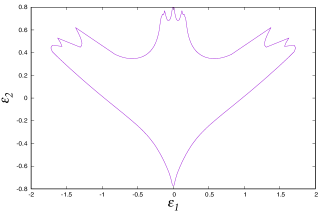
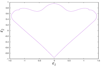
Figure 7: Existence domain for invariant circles of the dissipative standard map with potential (30). Left: $\lambda=0.9$. Right: $\lambda=0.1$.

We call attention to the fact that this region contains parts with smooth boundaries, but – specially in the conservative case – it contains some parts of the boundary that are rather ragged. A tentative explanation ([75]) is that the smooth parts of the the boundary of the region of existence are the intersection of the family considered with the stable manifold of fixed point of renormalization. Even if this is not a completely rigorous picture, there has been significant mathematical progress in verifying it in an open set of families. We hope that, in the future there could be more progress in this area.

One important advantage of the Sobolev method is that it can be programmed systematically and run unattended. The Greene’s method relies on periodic orbits and one has to pay attention to making sure that the periodic orbits are continued correctly. We also note that the Sobolev method works for models of long range interaction in Statistical Mechanics without a dynamical interpretation.

5.2 Greene’s method, periodic orbits and Arnold’s tongues

The method developed by J. Greene in [52] is based on the conjecture that the breakdown of an invariant curve with frequency $\omega$, say $\mathcal{C}(\omega)$, is related to a change from stability to instability of the periodic orbits $\mathcal{P}({{p_{j}}\over{q_{j}}})$ with frequencies ${{p_{j}}\over{q_{j}}}$ tending to $\omega$. We observe that a standard procedure to obtain the rational approximants of $\omega$ is to compute the successive truncations of the continued fraction representation of $\omega$.

Greene’s method has been successfully developed for the conservative standard map for which a partial justification is given in [47, 75]. In the dissipative case, there appears an extra difficulty due to the fact that the periodic orbits with frequency ${{p_{j}}\over{q_{j}}}$ occur in a whole interval of the drift parameter. This phenomenon gives rise to the appearance of the so-called Arnold tongues. Figure 8, left panel, gives a graphical representation of the Arnold tongues; having fixed a value of the dissipative parameter $\varepsilon$, there is a whole interval of the drift parameter $\mu$ which admits a periodic orbit of the same period. The right panel of Figure 8 shows several periodic orbits approaching the torus with frequency equal to the golden mean; such periodic orbits have frequency equal to the rational approximants which are given by the ratio of the Fibonacci numbers.

A partial justification of an extension of Greene’s criterion in the conformally symplectic case is presented in [23], where it is proved that if there exists a smooth invariant attractor, one can predict the eigenvalues of the periodic orbits approximating the torus for parameters close to those of the attractor.

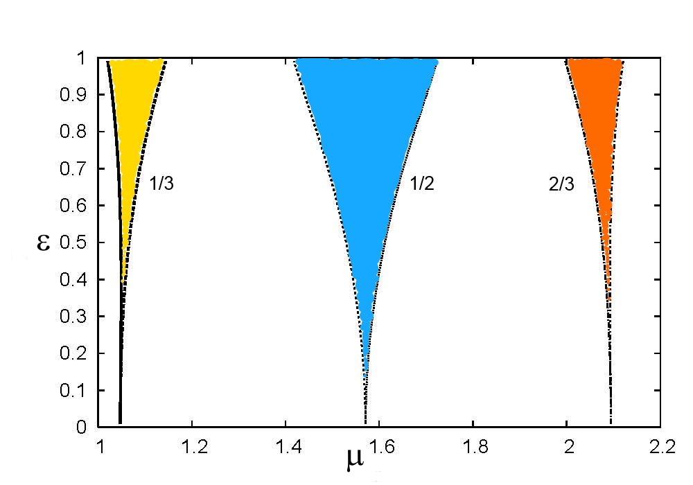
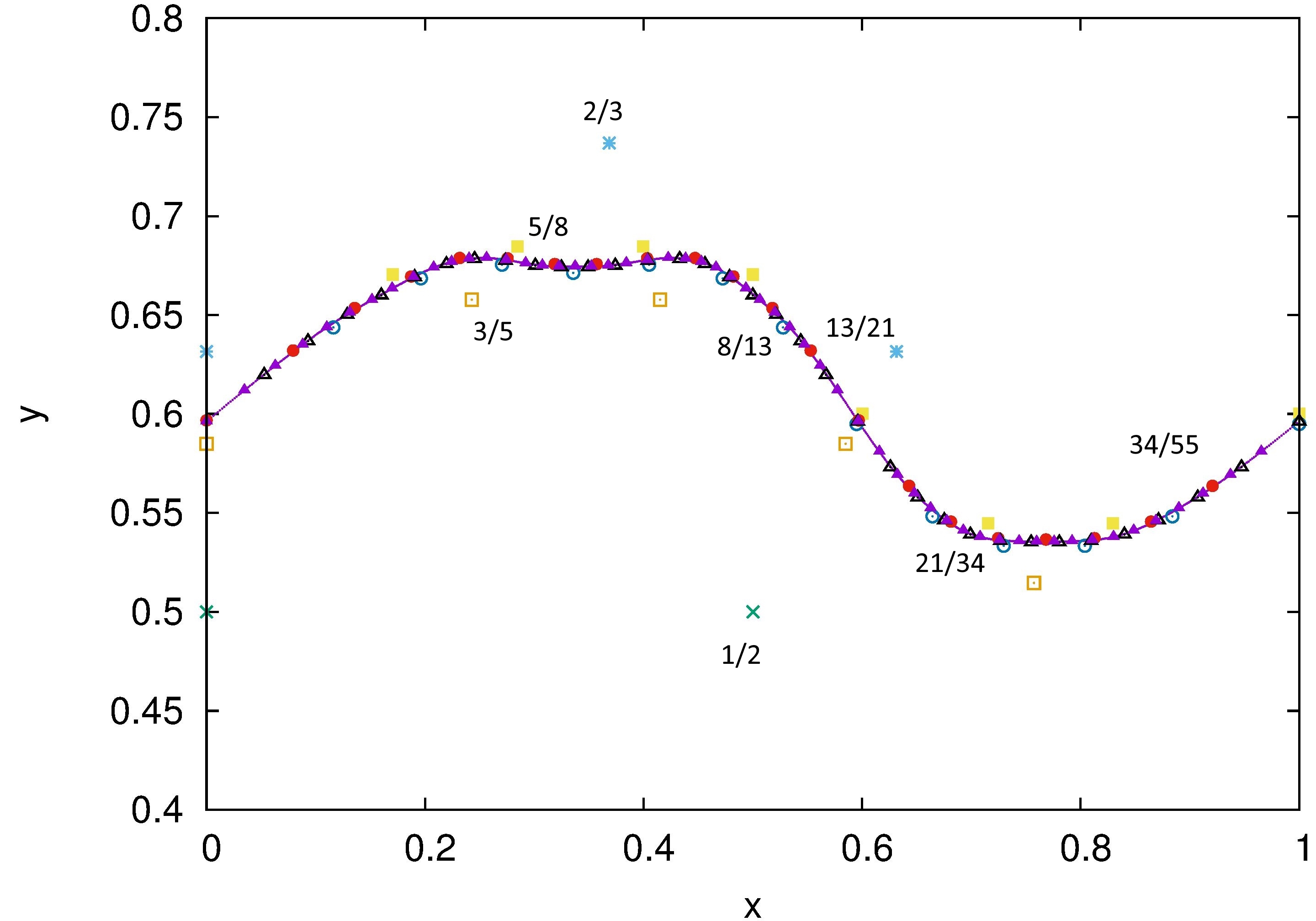
Figure 8: Left: Arnold’s tongues providing $\mu$ vs. $\varepsilon$ for three periodic orbits of the dissipative standard map with periods 1/3, 1/2, 2/3. Right: periodic orbits of the dissipative standard map approximating the golden mean curve.

Figure 9 shows some approximating periodic orbits (left panels) and the corresponding behaviour of the drift parameter (right panels) that, in the limit, tends to the value of the drift that corresponds to the golden mean torus.

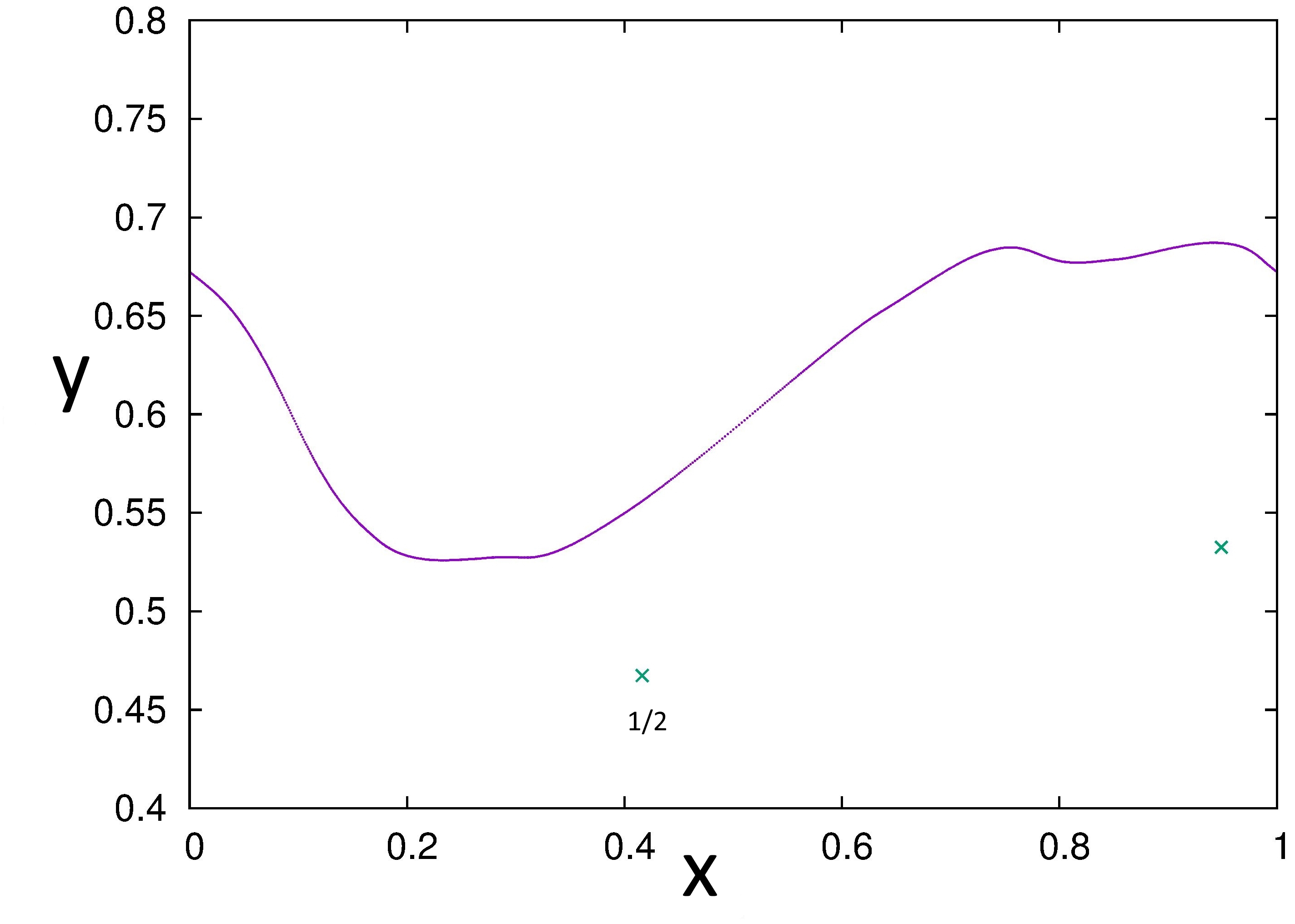
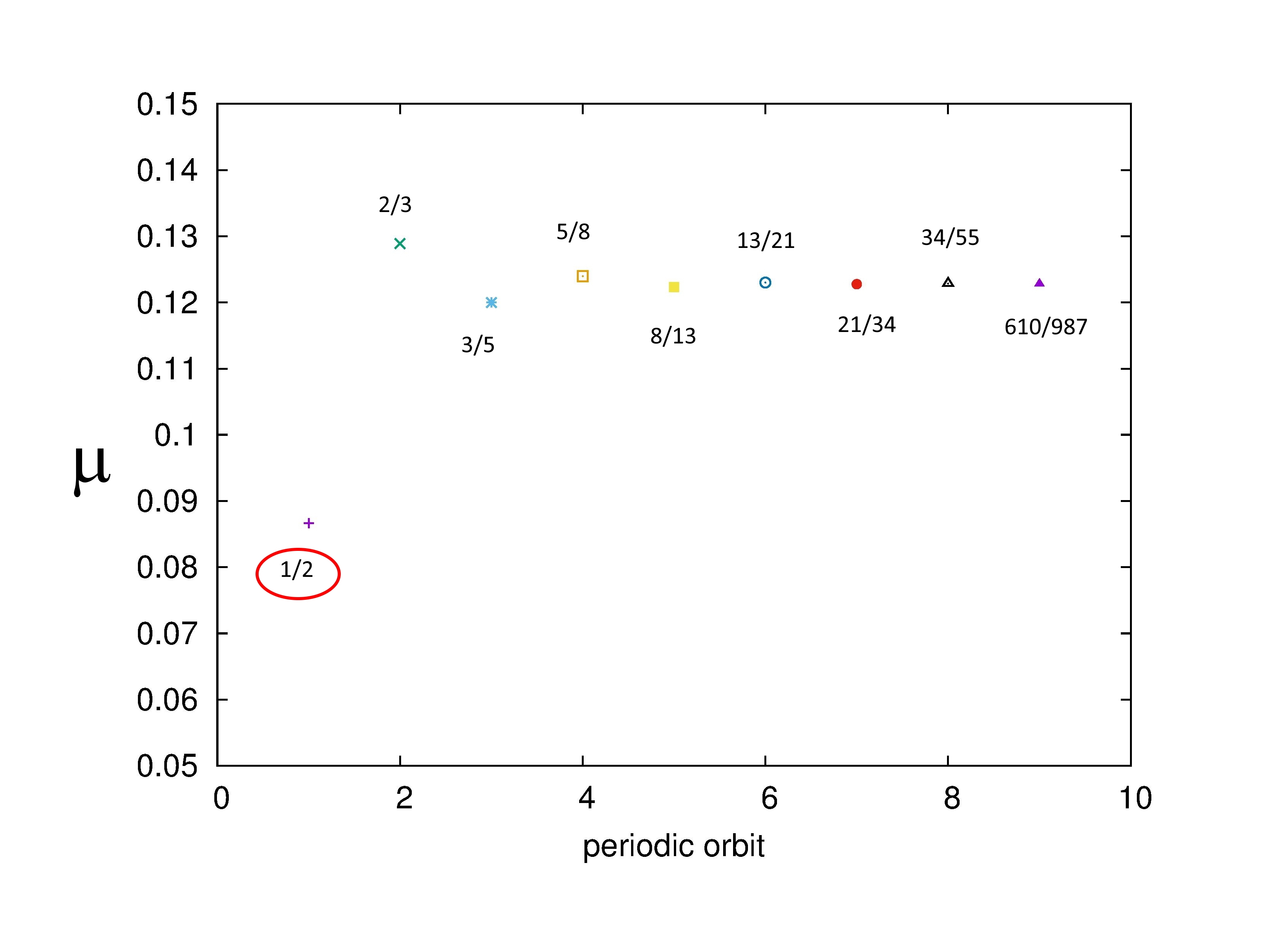
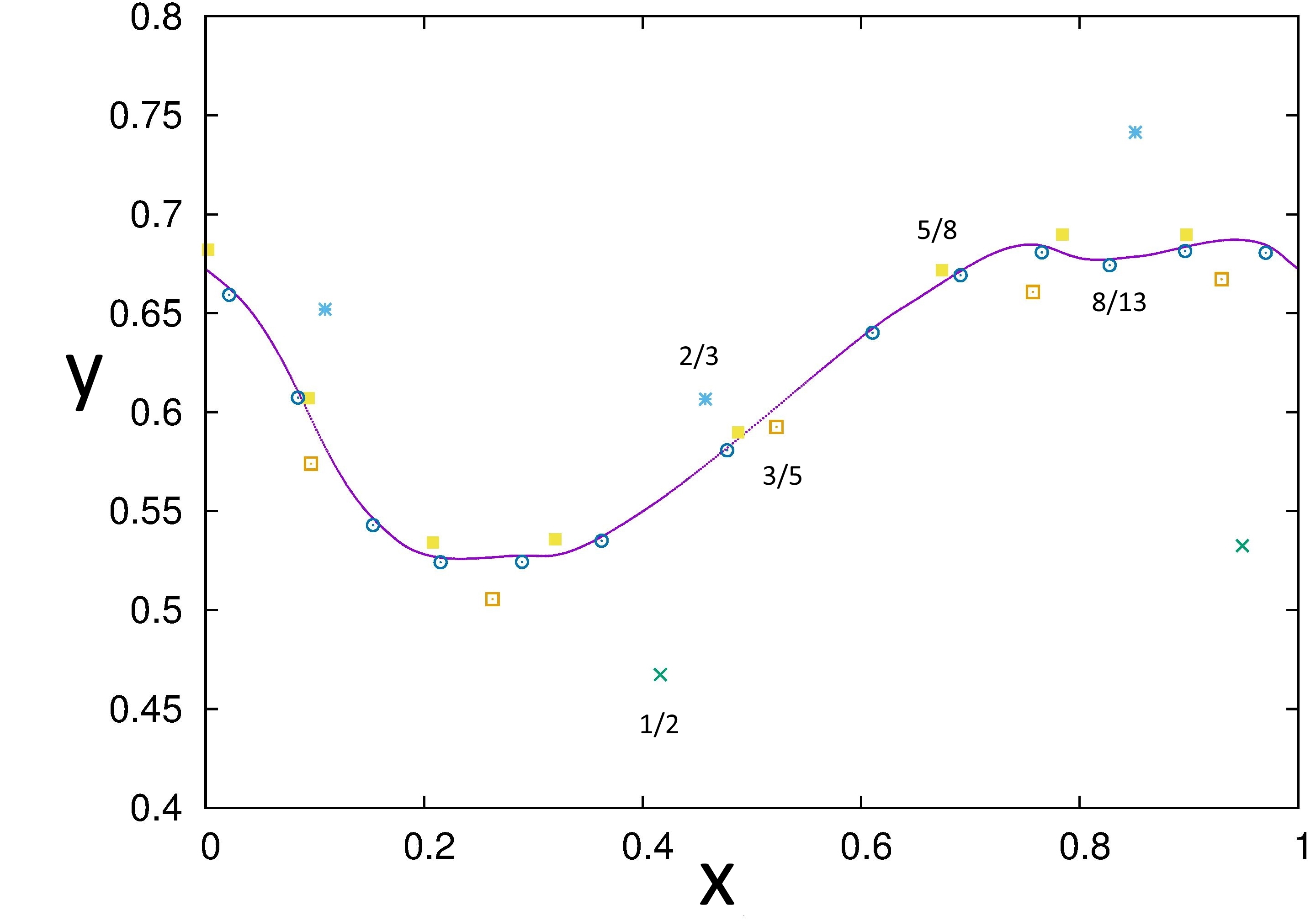
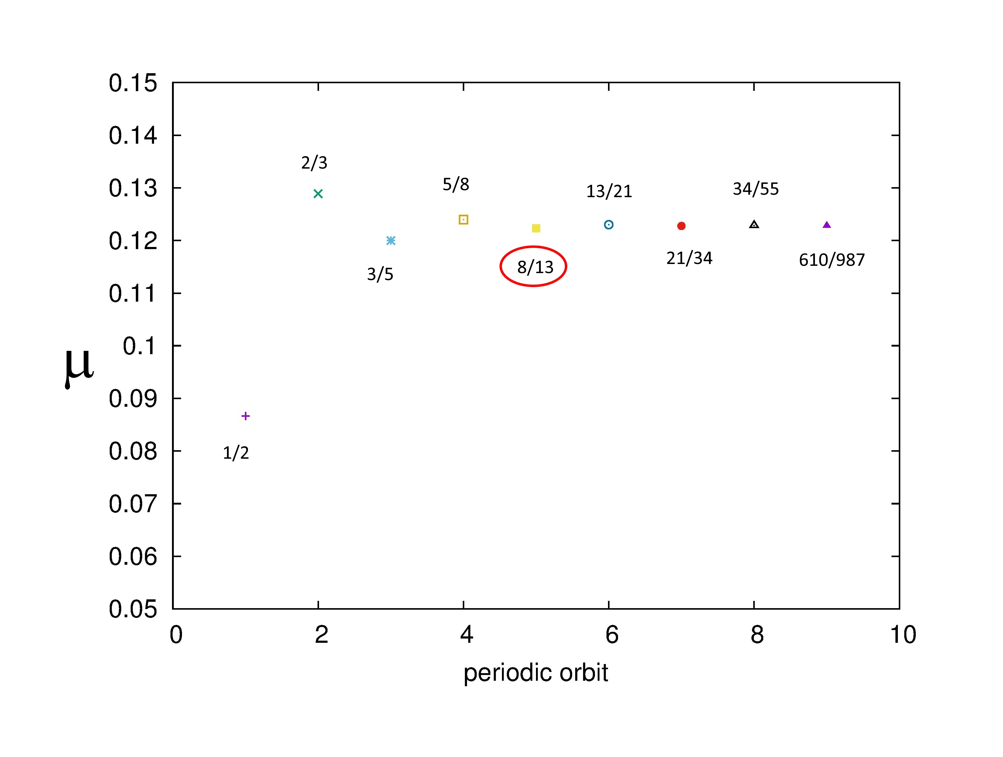
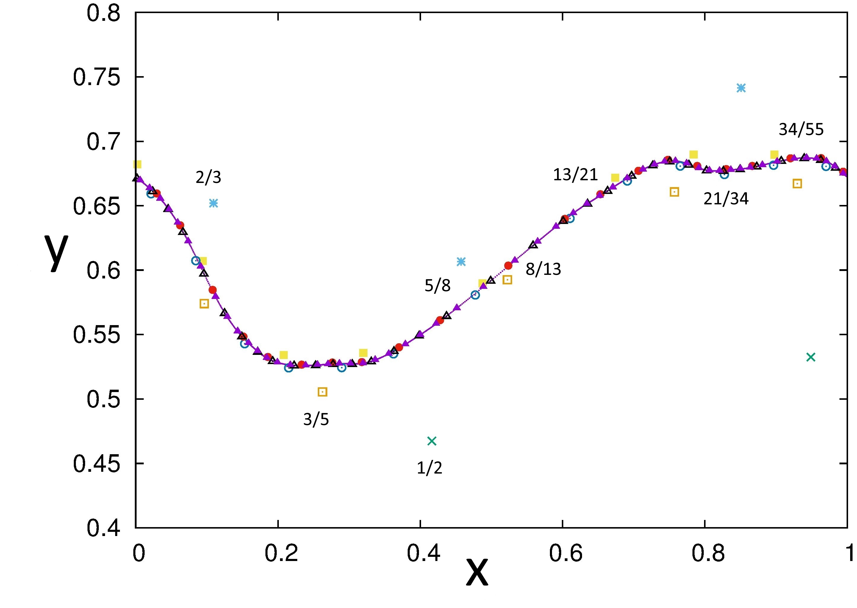
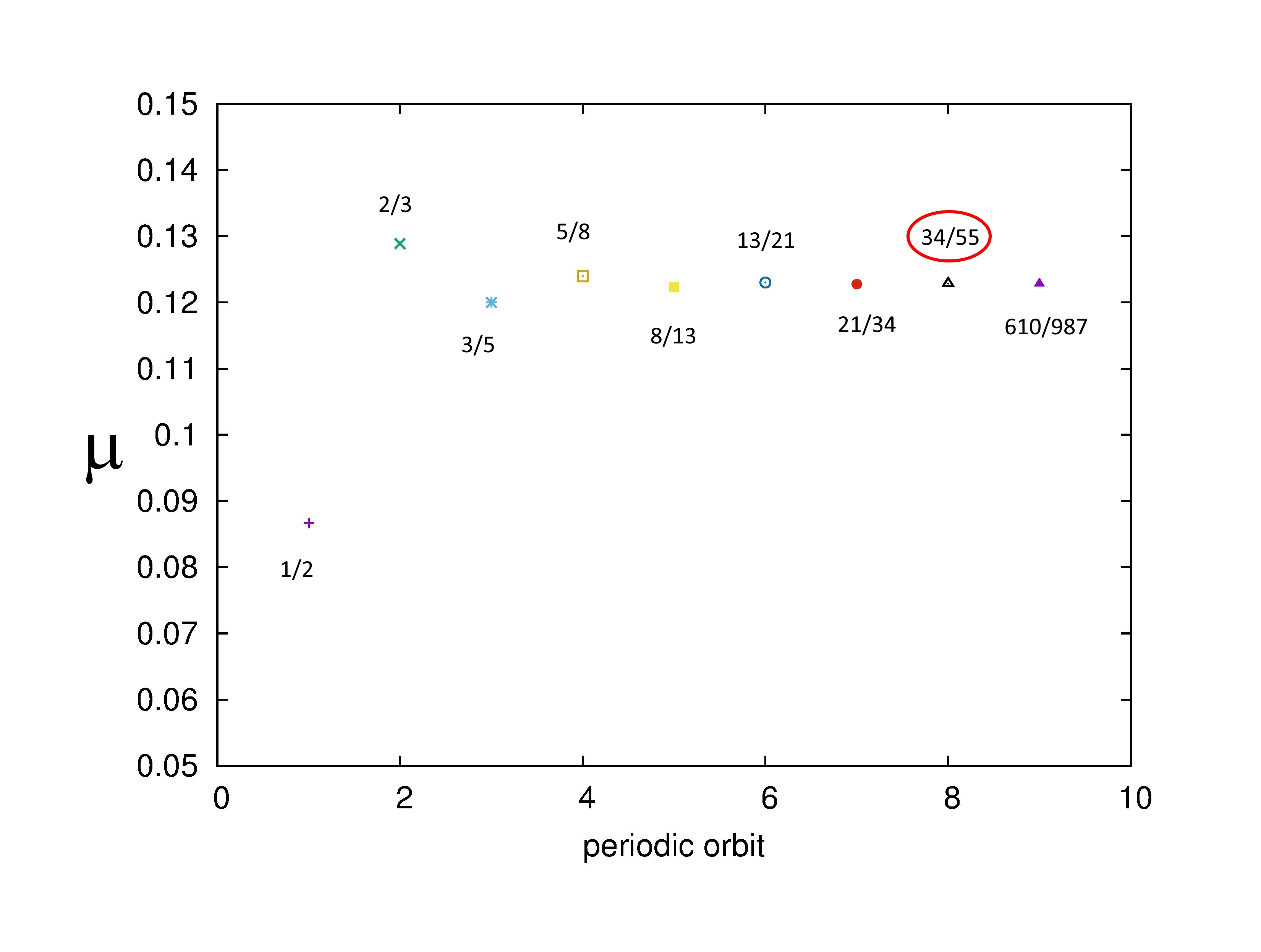
Figure 9: Left: periodic orbits with increasing periods, approximating the golden mean curve. Right: the corresponding drift parameters with the successive periodic orbits labeled by integer numbers on the $x$-axis.

We also call attention to [33] which contains tentative results on the non-existence of invariant tori for the spin-orbit models. Even if the methods developed there are not rigorous, they may present a counterpoint to the methods to study the existence.

6 Collision of invariant bundles of quasi-periodic attractors

Quasi-periodic attractors of conformally symplectic maps are normally hyperbolic invariant manifolds (NHIM). We can obtain the Lyapunov multipliers of the attractor from a simple computation. We start from the invariance equation (29) for a pair $(K,\mu)$. We then introduce a change of variables to reduce the cocycle. Let $\tilde{M}({\underline{\theta}})=[DK({\underline{\theta}})\,|\,E^{s}({\underline{\theta}})]$ be the matrix whose columns are the tangent and stable bundles of $\mathcal{K}=K(\mathbb{T}^{n})$:

$$Df_{\mu}\circ K({\underline{\theta}})\tilde{M}({\underline{\theta}})=\tilde{M}({\underline{\theta}}+{\underline{\omega}})\left(\begin{array}[]{cc}1&0\\ 0&\lambda\\ \end{array}\right)\ .$$ (31)

From equation (31) we can write the stable bundle as follows

$$E^{s}({\underline{\theta}})=DK({\underline{\theta}})B({\underline{\theta}})+J^{-1}DK({\underline{\theta}})N({\underline{\theta}})\ ,$$

where $B({\underline{\theta}})$ is the function that satisfies

$$B({\underline{\theta}})-\lambda B({\underline{\theta}}+{\underline{\omega}})=-S({\underline{\theta}})\ .$$

Indeed, after $j$ iterates of the map we have that,

$$Df_{\mu}^{j}\circ K({\underline{\theta}})=\tilde{M}({\underline{\theta}}+{\underline{\omega}})\left(\begin{array}[]{cc}1&0\\ 0&\lambda^{j}\\ \end{array}\right)\ \tilde{M}^{-1}({\underline{\theta}})\ ,$$

which shows that the tangent space of $\mathcal{M}$ at $K(\theta)$ is

$$T_{K(\theta)}\mathcal{M}=\mathrm{Range}(DK(\theta))\oplus E_{K(\theta)}^{s}\ .$$

We can conclude that there exists a constant $C$ such that

$$C^{-1}\lambda^{j}|v|\leq|Df_{\mu}^{j}\circ K({\underline{\theta}})\ v|\leq C\lambda^{j}|v|\ ,\qquad v\in E^{s}_{K({\underline{\theta}})}\ ,$$

$$C^{-1}\ |v|\leq|Df_{\mu}^{j}\circ K({\underline{\theta}})\ v|\leq C\ |v|\ ,\qquad\ v\in E^{c}_{K({\underline{\theta}})}\ ,$$

showing that $\mathcal{K}=K(\mathbb{T}^{n})$ is a NHIM. Equation (31) also tells us that the Lyapunov multipliers are constant along the family of quasi-periodic attractors for fixed Diophantine vectors.

In the case of maps of the cylinder $\mathcal{M}=\mathbb{R}\times\mathbb{T}$, we know that the curve $\mathcal{K}$ is $C^{r}$, one dimensional, and since $\omega$ satisfies the Diophantine condition, we know by the results of [56, 61, 59, 58] that the map conjugating the dynamics in $\mathcal{K}$ to a rigid rotation is in $C^{r-\tau-\delta}$ for a small $\delta>0$. Therefore, by the bootstrap of regularity results, the conjugacy is analytic for analytic maps. Since the bundles depend on the conjugacy, then the regularity of the manifold implies the analyticity of $K$ and the bundles up to the breakdown.

To investigate the breakdown of normal hyperbolicity, we note that, because of the pairing rule of Lyapunov exponents [46, 99], since one Lyapunov multiplier is $1$ – the one along the tangent directional (remember that the map on the torus is smoothly conjugate to the torus) – the other one is precisely $\lambda$.

We recall that hyperbolicity is equivalent to the existence of transversal invariant bundles with different rates. In our case, if the tori have to cease to be normally hyperbolic, because the exponents remain constant, the only thing that can happen is that the transversality of the bundles deteriorates.

What is found empirically is that the breakdown happens because at the same time the regularity of the conjugacy deteriorates quantitatively (even if the conjugacy remains analytic, some Sobolev norm blows up).

At the same parameter values, the breakdown of hyperbolicity happens via the stable and tangent bundle collision. Even if the Lyapunov exponents remain safely away, the transversality deteriorates and the tangent and stable bundles become close to tangent.

In the case at hand, we can make a very detailed study: the bundles are one dimensional and we compute a formula for the angle between the bundles for every $\theta$. In fact, let $\alpha(\theta)$ be the angle between the stable and tangent bundles for every $\theta\in\mathbb{T}$, then we have

$$\alpha(\theta)=\arctan\left(\frac{1}{B(\theta)(DK(\theta)^{T}DK(\theta))}\right).$$

This formula says that the angle $\alpha(\theta)$ goes to zero at points where the functions in the denominator go to infinity.

We present figures (see Figure 10) of the angle between the bundles close to the breakdown.

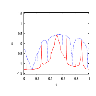
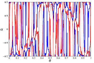
Figure 10: Invariant bundles close to their collision. Left: dissipative standard map. Right: dissipative standard non-twist map. Reproduced from [13].

Rather remarkably these two phenomena (the blow up of Sobolev norms and the stable bundles and the tangent becoming parallel) happen at the same time and present very unexpected regularities. There are scaling relations that seem to be independent of the family considered and they happen in codimension $1$ smooth submanifolds in the space of maps. We think that this is a very interesting mathematical phenomenon that deserves rigorous study. It seems quite unlikely that it would have been discovered except for the very careful numerics that can explore with confidence close to the breakdown. Such delicate numerics are only possible because of the rigorous mathematical development.

7 Applications

In this Section we want to briefly review some applications of KAM theory for conservative and dissipative models. We will consider applications to the standard map and to the spin-orbit problem, both in the conservative and dissipative settings. Although we will not present other applications of KAM theory, it is worth mentioning also the constructive KAM results to the N-body and planetary problems in Celestial Mechanics ([81]); in this context, for results obtained in the conservative framework we refer the reader to [2, 26, 27, 28, 89, 51] and to [34] for numerical investigations including dissipative effects.

7.1 Applications to the standard maps

The first applications of computer-assisted KAM proofs have been given for the conservative standard map; these results show that the golden mean torus persists for values of the perturbing parameter equal to $93\%$ of the numerical breakdown value (see [41, 40]); we also mention [25] which, at the same epoch but using a different approach than [41, 40], reached $86\%$ of the numerical breakdown value.

Rigorous estimates for the conservative standard map using the a-posteriori method have been proved in the remarkable paper [49], where for the twist and non-twist conservative standard maps the golden mean torus is proved to persist for values of the perturbing parameter as high as 99.9% of the numerical breakdown value.

For the dissipative standard map, the paper [21] analyzes the persistence of the invariant attractor with frequency equal to the golden mean and for a fixed value of the dissipative parameter (precisely $\lambda=0.9$); such persistence is shown for values of the perturbing parameter equal to 99.9% of the breakdown value, where the numerical value has been obtained through the techniques presented in Sections 5.1 and 5.2.

7.2 Applications to the spin–orbit problems

The first application of KAM theory to the conservative spin-orbit problem is found in [30, 29]. In those articles some satellites in synchronous spin-orbit resonance have been considered; the synchronous or 1:1 spin-orbit resonance implies that the satellite always points the same face to the host planet. In particular, the following satellites have been considered: the Moon, and three satellites of Saturn, Rhea, Enceladus, Dione. Being the normalized frequency (namely, the ratio between the rotational and orbital frequency) equal to one, two Diophantine numbers bounding unity from above and below have been considered. Through a computer-assisted KAM theorem, the existence of invariant tori with frequency equal to the bounding numbers have been established for the true values of the parameters of the satellites, namely the eccentricity and the equatorial oblateness.

Such result guarantees the stability for infinite times in the sense of confinement in the phase space. In fact, the phase space associated to the Hamiltonian describing the conservative spin-orbit problem is 3-dimensional; since the KAM tori are 2-dimensional, one gets a confinement of the motion between the bounding invariant tori.

We remark that the confinement is no more valid for $n>2$ degrees of freedom, since the motion can diffuse through invariant tori, reaching arbitrarily far regions; this phenomenon is known as Arnold’s diffusion ([3]) for which we refer to the extensive literature on this topic (see, e.g., [44, 50] and references therein).

For the dissipative spin-orbit problem, we refer to [32] for the development of KAM theory for a model of spin-orbit interaction with tidal torque as in (2.3). Precisely, for $\lambda_{0}\in{\mathbb{R}_{+}}$ and $\omega$ Diophantine, it is proven that there exists $0<\varepsilon_{0}<1$, such that for any $\varepsilon\in[0,\varepsilon_{0}]$ and any $\lambda\in[-\lambda_{0},\lambda_{0}]$ there exists a unique function $K=K(\theta,t)$ and a drift term $\mu$ which is the solution of the invariance equation for the dissipative spin-orbit model.

Explicit estimates for the dissipative spin-orbit problem, even in the more general case with a time-dependent tidal torque as in (9), are given in [24] (see also [91]). Here, the a-posteriori method is implemented to construct invariant attractors with Diophantine frequency; the results are valid for values of the perturbing parameter consistent with the astronomical values of the Moon and very close to the numerical breakdown threshold, which has been computed in [24] through Sobolev and Greene’s method (see also [92]).

Acknowledgements. R.C. was partially supported by DGAPA-UNAM Project IN 101020. A.C. acknowledges the MIUR Excellence Department Project awarded to the Department of Mathematics, University of Rome Tor Vergata, CUP E83C18000100006, EU-ITN Stardust-R, MIUR-PRIN 20178CJA2B “New Frontiers of Celestial Mechanics: theory and Applications”. R.L was partially supported by NSF grant DMS 1800241.

References

- [1] V. I. Arnol’d. Proof of a theorem of A. N. Kolmogorov on the invariance of quasi-periodic motions under small perturbations. Russian Math. Surveys, 18(5):9–36, 1963.
- [2] V. I. Arnol’d. Small denominators and problems of stability of motion in classical and celestial mechanics. Russian Math. Surveys, 18(6):85–191, 1963.
- [3] V.I. Arnold. Instability of dynamical systems with several degrees of freedom. Sov. Math. Doklady, 5:581–585, 1964.
- [4] A. Banyaga. Some properties of locally conformal symplectic structures. Comment. Math. Helv., 77(2):383–398, 2002.
- [5] Alain Bensoussan. Perturbation methods in optimal control. Wiley/Gauthier-Villars Series in Modern Applied Mathematics. John Wiley & Sons Ltd., Chichester, 1988. Translated from the French by C. Tomson.
- [6] Tomas Bohr. A bound for the existence of invariant circles in a class of two-dimensional dissipative maps. Phys. Lett. A, 104(9):441–443, 1984.
- [7] Tomas Bohr, Per Bak, and Mogens Hogh Jensen. Transition to chaos by interaction of resonances in dissipative systems. II. Josephson junctions, charge-density waves, and standard maps. Phys. Rev. A (3), 30(4):1970–1981, 1984.
- [8] H. W. Broer, G. B. Huitema, and M. B. Sevryuk. Families of quasi-periodic motions in dynamical systems depending on parameters. In Nonlinear dynamical systems and chaos (Groningen, 1995), pages 171–211. Birkhäuser, Basel, 1996.
- [9] H. W. Broer, G. B. Huitema, and M. B. Sevryuk. Quasi-Periodic Motions in Families of Dynamical Systems. Order Amidst Chaos. Springer-Verlag, Berlin, 1996.
- [10] H. W. Broer, G. B. Huitema, F. Takens, and B. L. J. Braaksma. Unfoldings and bifurcations of quasi-periodic tori. Mem. Amer. Math. Soc., 83(421):viii+175, 1990.
- [11] Adrián P. Bustamante and Renato C. Calleja. Computation of domains of analyticity for the dissipative standard map in the limit of small dissipation. Phys. D, 395:15–23, 2019.
- [12] Adrián P. Bustamante and Rafael de la Llave. Gevrey estimates for the asymptotic expansion of tori of weakly dissipative systems. Preprint, 2020.
- [13] R. Calleja, M. Canadell, and A. Haro. Non-twist tori in conformally symplectic systems. Preprint, 2020.
- [14] R. Calleja and A. Celletti. Breakdown of invariant attractors for the dissipative standard map. Chaos, 20(1):013121, 2010.
- [15] R. Calleja and R. de la Llave. A numerically accessible criterion for the breakdown of quasi-periodic solutions and its rigorous justification. Nonlinearity, 23(9):2029–2058, 2010.
- [16] Renato Calleja and Jordi-Lluis Figueras. Collision of invariant bundles of quasi-periodic attractors in the dissipative standard map. Chaos, 22(3):033114, 10, 2012.
- [17] Renato C. Calleja, Alessandra Celletti, and Rafael de la Llave. A KAM theory for conformally symplectic systems: efficient algorithms and their validation. J. Differential Equations, 255(5):978–1049, 2013.
- [18] Renato C. Calleja, Alessandra Celletti, and Rafael de la Llave. Local behavior near quasi-periodic solutions of conformally symplectic systems. J. Dynam. Differential Equations, 25(3):821–841, 2013.
- [19] Renato C. Calleja, Alessandra Celletti, and Rafael de la Llave. Domains of analyticity and Lindstedt expansions of KAM tori in some dissipative perturbations of Hamiltonian systems. Nonlinearity, 30(8):3151–3202, 2017.
- [20] Renato C. Calleja, Alessandra Celletti, and Rafael de la Llave. Existence of whiskered KAM tori of conformally symplectic systems. Nonlinearity, 33(1):538–597, 2020.
- [21] Renato C. Calleja, Alessandra Celletti, and Rafael de la Llave. KAM estimates for the dissipative standard map. Preprint, 2020.
- [22] Renato C. Calleja, Alessandra Celletti, and Rafael de la Llave. Whiskered KAM tori of conformally symplectic systems. Mathematics Research Reports, 1:15–29, 2020.
- [23] Renato C. Calleja, Alessandra Celletti, Corrado Falcolini, and Rafael de la Llave. An Extension of Greene’s Criterion for Conformally Symplectic Systems and a Partial Justification. SIAM J. Math. Anal., 46(4):2350–2384, 2014.
- [24] Renato C. Calleja, Alessandra Celletti, Joan Gimeno, and Rafael de la Llave. Breakdown threshold and KAM estimates in the spin-orbit problem with tidal torque. Preprint, 2020.
- [25] A. Celletti and L. Chierchia. A constructive theory of Lagrangian tori and computer-assisted applications. In Dynamics Reported, pages 60–129. Springer, Berlin, 1995.
- [26] A. Celletti and L. Chierchia. On the stability of realistic three-body problems. Comm. Math. Phys., 186(2):413–449, 1997.
- [27] A. Celletti and L. Chierchia. KAM tori for -body problems: a brief history. Celestial Mech. Dynam. Astronom., 95(1-4):117–139, 2006.
- [28] A. Celletti and L. Chierchia. KAM stability and celestial mechanics. Memoirs of the Americal Mathematical Society, 187(878), 2007.
- [29] Alessandra Celletti. Analysis of resonances in the spin-orbit problem in celestial mechanics: higher order resonances and some numerical experiments. II. Z. Angew. Math. Phys., 41(4):453–479, 1990.
- [30] Alessandra Celletti. Analysis of resonances in the spin-orbit problem in celestial mechanics: the synchronous resonance. I. Z. Angew. Math. Phys., 41(2):174–204, 1990.
- [31] Alessandra Celletti. Stability and Chaos in Celestial Mechanics. Springer-Verlag, Berlin; published in association with Praxis Publishing, Chichester, 2010.
- [32] Alessandra Celletti and Luigi Chierchia. Quasi-periodic attractors in celestial mechanics. Arch. Ration. Mech. Anal., 191(2):311–345, 2009.
- [33] Alessandra Celletti and Robert MacKay. Regions of nonexistence of invariant tori for spin-orbit models. Chaos, 17(4):043119, 12, 2007.
- [34] Alessandra Celletti, Letizia Stefanelli, Elena Lega, and Claude Froeschlé. Some results on the global dynamics of the regularized restricted three-body problem with dissipation. Celestial Mech. Dynam. Astronom., 109(3):265–284, 2011.
- [35] L. Chierchia and G. Gallavotti. Smooth prime integrals for quasi-integrable Hamiltonian systems. Nuovo Cimento B (11), 67(2):277–295, 1982.
- [36] B.V. Chirikov. A universal instability of many-dimensional oscillator systems. Phys. Rep., 52(5):264–379, 1979.
- [37] Alexandre C. M. Correia and Jacques Laskar. Mercury’s capture into the 3/2 spin-orbit resonance as a result of its chaotic dynamics. Nature, 429(6994):848–850, 2004.
- [38] R. de la Llave. A tutorial on KAM theory. In Smooth ergodic theory and its applications (Seattle, WA, 1999), pages 175–292. Amer. Math. Soc., Providence, RI, 2001.
- [39] R. de la Llave, A. González, À. Jorba, and J. Villanueva. KAM theory without action-angle variables. Nonlinearity, 18(2):855–895, 2005.
- [40] R. de la Llave and D. Rana. Accurate strategies for small divisor problems. Bull. Amer. Math. Soc. (N.S.), 22(1):85–90, 1990.
- [41] R. de la Llave and D. Rana. Accurate strategies for K.A.M. bounds and their implementation. In Computer Aided Proofs in Analysis (Cincinnati, OH, 1989), pages 127–146. Springer, New York, 1991.
- [42] D. del Castillo-Negrete, J. M. Greene, and P. J. Morrison. Area preserving nontwist maps: periodic orbits and transition to chaos. Phys. D, 91(1-2):1–23, 1996.
- [43] D. del Castillo-Negrete, J. M. Greene, and P. J. Morrison. Renormalization and transition to chaos in area preserving nontwist maps. Phys. D, 100(3-4):311–329, 1997.
- [44] Amadeu Delshams, Rafael de la Llave, and Tere M. Seara. A geometric mechanism for diffusion in Hamiltonian systems overcoming the large gap problem: heuristics and rigorous verification on a model. Mem. Amer. Math. Soc., 179(844):viii+141, 2006.
- [45] C. P. Dettmann and G. P. Morris. Proof of Lyapunov exponent pairing for systems at constant kinetic energy. Phys. Rev. E, 53(6):R5545–R5548, 2006.
- [46] C. P. Dettmann and G. P. Morriss. Hamiltonian formulation of the Gaussian isokinetic thermostat. Phys. Rev. E, 54:2495–2500, Sep 1996.
- [47] Corrado Falcolini and Rafael de la Llave. A rigorous partial justification of Greene’s criterion. J. Statist. Phys., 67(3-4):609–643, 1992.
- [48] Ulrike Feudel, Celso Grebogi, Brian R. Hunt, and James A. Yorke. Map with more than coexisting low-period periodic attractors. Phys. Rev. E (3), 54(1):71–81, 1996.
- [49] J.-Ll. Figueras, A. Haro, and A. Luque. Rigorous computer-assisted application of KAM theory: a modern approach. Found. Comput. Math., 17(5):1123–1193, 2017.
- [50] Marian Gidea, Rafael de la Llave, and Tere M-Seara. A general mechanism of diffusion in Hamiltonian systems: qualitative results. Comm. Pure Appl. Math., 73(1):150–209, 2020.
- [51] Antonio Giorgilli, Ugo Locatelli, and Marco Sansottera. An extension of Lagrange’s theory for secular motions. Rend. Cl. Sci. Mat. Nat., 143:223–239, 2009.
- [52] J. M. Greene. A method for determining a stochastic transition. Jour. Math. Phys., 20:1183–1201, 1979.
- [53] John Guckenheimer and Philip Holmes. Nonlinear oscillations, dynamical systems, and bifurcations of vector fields, volume 42 of Applied Mathematical Sciences. Springer-Verlag, New York, 1990. Revised and corrected reprint of the 1983 original.
- [54] A. Haro. Automatic differentiation tools in computational dynamical systems. Work in progress, 2011.
- [55] Àlex Haro, Marta Canadell, Jordi-Lluís Figueras, Alejandro Luque, and Josep-Maria Mondelo. The parameterization method for invariant manifolds, volume 195 of Applied Mathematical Sciences. Springer, [Cham], 2016. From rigorous results to effective computations.
- [56] M.-R. Herman. Sur la conjugaison différentiable des difféomorphismes du cercle à des rotations. Inst. Hautes Études Sci. Publ. Math., (49):5–233, 1979.
- [57] I. Jungreis. A method for proving that monotone twist maps have no invariant circles. Ergodic Theory Dynamical Systems, 11(1):79–84, 1991.
- [58] Y. Katznelson and D. Ornstein. The absolute continuity of the conjugation of certain diffeomorphisms of the circle. Ergodic Theory Dynamical Systems, 9(4):681–690, 1989.
- [59] Y. Katznelson and D. Ornstein. The differentiability of the conjugation of certain diffeomorphisms of the circle. Ergodic Theory Dynamical Systems, 9(4):643–680, 1989.
- [60] Jukka A. Ketoja and Indubala I. Satija. Harper equation, the dissipative standard map and strange nonchaotic attractors: relationship between an eigenvalue problem and iterated maps. volume 109, pages 70–80. 1997. Physics and dynamics between chaos, order, and noise (Berlin, 1996).
- [61] K. M. Khanin and Ya. G. Sinai. A new proof of M. Herman’s theorem. Comm. Math. Phys., 112(1):89–101, 1987.
- [62] Sang-Yoon Kim and Duck-Sung Lee. Transition to chaos in a dissipative standardlike map. Phys. Rev. A (3), 45(8):5480–5487, 1992.
- [63] H. Koch. A renormalization group for Hamiltonians, with applications to KAM tori. Ergodic Theory Dynam. Systems, 19:1–47, 1999.
- [64] H. Koch, A. Schenkel, and P. Wittwer. Computer-assisted proofs in analysis and programming in logic: a case study. SIAM Rev., 38(4):565–604, 1996.
- [65] Hans Koch. A renormalization group fixed point associated with the breakup of golden invariant tori. Discrete Contin. Dyn. Syst., 11(4):881–909, 2004.
- [66] Hans Koch. Existence of critical invariant tori. Ergodic Theory Dynam. Systems, 28(6):1879–1894, 2008.
- [67] Hans Koch. On hyperbolicity in the renormalization of near-critical area-preserving maps. Discrete Contin. Dyn. Syst., 36(12):7029–7056, 2016.
- [68] A. N. Kolmogorov. On conservation of conditionally periodic motions for a small change in Hamilton’s function. Dokl. Akad. Nauk SSSR (N.S.), 98:527–530, 1954. English translation in Stochastic Behavior in Classical and Quantum Hamiltonian Systems (Volta Memorial Conf., Como, 1977), Lecture Notes in Phys., 93, pages 51–56. Springer, Berlin, 1979.
- [69] W. T. Kyner. Rigorous and formal stability of orbits about an oblate planet. Mem. Amer. Math. Soc. No. 81. Amer. Math. Soc., Providence, R.I., 1968.
- [70] Oscar E. Lanford, III. Computer-assisted proofs in analysis. In Proceedings of the International Congress of Mathematicians, Vol. 1, 2 (Berkeley, Calif., 1986), pages 1385–1394, Providence, RI, 1987. Amer. Math. Soc.
- [71] J. Laskar, C. Froeschlé, and A. Celletti. The measure of chaos by the numerical analysis of the fundamental frequencies. application to the standard mapping. Physica D, 56:253–269, 1992.
- [72] M. Levi. Qualitative analysis of the periodically forced relaxation oscillations. Mem. Amer. Math. Soc., 32(244):vi+147, 1981.
- [73] A. J. Lichtenberg and M. A. Lieberman. Regular and chaotic dynamics, volume 38 of Applied Mathematical Sciences. Springer-Verlag, New York, second edition, 1992.
- [74] Kevin K. Lin and Lai-Sang Young. Shear-induced chaos. Nonlinearity, 21(5):899–922, 2008.
- [75] R. S. MacKay. Greene’s residue criterion. Nonlinearity, 5(1):161–187, 1992.
- [76] R. S. McKay. Renormalisation in Area Preserving Maps. PhD thesis, Princeton University, 1982.
- [77] K. R. Meyer. Lie transform tutorial. II. In Computer Aided Proofs in Analysis (Cincinnati, OH, 1989), pages 190–210. Springer, New York, 1991.
- [78] J. Moser. On invariant curves of area-preserving mappings of an annulus. Nachr. Akad. Wiss. Göttingen Math.-Phys. Kl. II, 1962:1–20, 1962.
- [79] J. Moser. Convergent series expansions for quasi-periodic motions. Math. Ann., 169:136–176, 1967.
- [80] S.J. Peale. The free precession and libration of Mercury. Icarus, 178:4–18, 2005.
- [81] H. Poincaré. New Methods of Celestial Mechanics. Vols. 1–3. American Institute of Physics, New York, 1993.
- [82] J. Pöschel. Integrability of Hamiltonian systems on Cantor sets. Comm. Pure Appl. Math., 35(5):653–696, 1982.
- [83] Jürgen Pöschel. A lecture on the classical KAM theorem. In Smooth ergodic theory and its applications (Seattle, WA, 1999), volume 69 of Proc. Sympos. Pure Math., pages 707–732. Amer. Math. Soc., Providence, RI, 2001.
- [84] D. Rana. Proof of Accurate Upper and Lower Bounds to Stability Domains in Small Denominator Problems. PhD thesis, Princeton University, 1987.
- [85] D. A. Rand. Existence, nonexistence and universal breakdown of dissipative golden invariant tori. I. Golden critical circle maps. Nonlinearity, 5(3):639–662, 1992.
- [86] D. A. Rand. Existence, nonexistence and universal breakdown of dissipative golden invariant tori. II. Convergence of renormalization for mappings of the annulus. Nonlinearity, 5(3):663–680, 1992.
- [87] D. A. Rand. Existence, nonexistence and universal breakdown of dissipative golden invariant tori. III. Invariant circles for mappings of the annulus. Nonlinearity, 5(3):681–706, 1992.
- [88] H. Rüssmann. On optimal estimates for the solutions of linear difference equations on the circle. Celestial Mech., 14(1):33–37, 1976.
- [89] M. Sansottera, U. Locatelli, and A. Giorgilli. On the stability of the secular evolution of the planar Sun-Jupiter-Saturn-Uranus system. Math. Comput. Simulation, 88:1–14, 2013.
- [90] G. Schmidt and B.W. Wang. Dissipative standard map. Physical Review A, 32(5):2994–2999, 1985. cited By 45.
- [91] Letizia Stefanelli and Ugo Locatelli. Kolmogorov’s normal form for equations of motion with dissipative effects. Discrete Contin. Dynam. Systems, 17(7):2561–2593, 2012.
- [92] Letizia Stefanelli and Ugo Locatelli. Quasi-periodic motions in a special class of dynamical equations with dissipative effects: A pair of detection methods. Discrete Contin. Dyn. Syst. Ser. B, 20(4):1155–1187, 2015.
- [93] Andreas Stirnemann. Renormalization for golden circles. Comm. Math. Phys., 152(2):369–431, 1993.
- [94] Andreas Stirnemann. Towards an existence proof of MacKay’s fixed point. Comm. Math. Phys., 188(3):723–735, 1997.
- [95] O. F. Vlasova and G. M. Zaslavsky. Nonergodic regions in the standard dissipative mapping. Phys. Lett. A, 105(1-2):1–5, 1984.
- [96] Qiudong Wang and Lai-Sang Young. Toward a theory of rank one attractors. Ann. of Math. (2), 167(2):349–480, 2008.
- [97] C. E. Wayne. An introduction to KAM theory. In Dynamical Systems and Probabilistic Methods in Partial Differential Equations (Berkeley, CA, 1994), pages 3–29. Amer. Math. Soc., Providence, RI, 1996.
- [98] W. Wenzel, O. Biham, and C. Jayaprakash. Periodic orbits in the dissipative standard map. Physical Review A, 43(12):6550–6557, 1991. cited By 34.
- [99] M. P. Wojtkowski and C. Liverani. Conformally symplectic dynamics and symmetry of the Lyapunov spectrum. Comm. Math. Phys., 194(1):47–60, 1998.
- [100] Y. Yamaguchi. Breakup of an invariant curve in a dissipative standard mapping. Physics Letters A, 116(7):307–310, 1986. cited By 1.