Self-Supervised Nuclei Segmentation in Histopathological Images Using Attention

Abstract

Segmentation and accurate localization of nuclei in histopathological images is a very challenging problem, with most existing approaches adopting a supervised strategy. These methods usually rely on manual annotations that require a lot of time and effort from medical experts. In this study, we present a self-supervised approach for segmentation of nuclei for whole slide histopathology images. Our method works on the assumption that the size and texture of nuclei can determine the magnification at which a patch is extracted. We show that the identification of the magnification level for tiles can generate a preliminary self-supervision signal to locate nuclei. We further show that by appropriately constraining our model it is possible to retrieve meaningful segmentation maps as an auxiliary output to the primary magnification identification task. Our experiments show that with standard post-processing, our method can outperform other unsupervised nuclei segmentation approaches and report similar performance with supervised ones on the publicly available MoNuSeg dataset. Our code and models are available online to facilitate further research.

1 Introduction

Histology images are the gold standard in diagnosing a considerable number of diseases including almost all types of cancer. For example, the count of nuclei on whole-slide images (WSIs) can have diagnostic significance for numerous cancerous conditions [20]. The proliferation of digital pathology and high-throughput tissue imaging leads to the adoption in clinical practice of digitized histopathological images that are utilized and archived every day. Such WSIs are acquired from glass histology slides using dedicated scanning devices after a staining process. In each WSI, thousands of nuclei from various types of cell can be identified. The detection of such nuclei is crucial for the identification of tissue structures, which can be further analyzed in a systematic manner and used for various clinical tasks. Presence, extent, size, shape, and other morphological characteristics of such structures are important indicators of the severity of different diseases [6]. Moreover, a quantitative analysis of digital pathology is important, to understand the underlying biological reasons for diseases [21].

Manual segmentation or estimation of nuclei on a WSI is an extremely time consuming process which suffers from high inter-observer variability [1]. On the other hand, data-driven methods that perform well on a specific histopathological datasets report poor performance on other datasets due again to the high variability in acquisition parameters and biological properties of cells in different organs and diseases [13]. To deal with this problem, datasets integrating different organs [13, 4] based on images from The Cancer Genome Atlas (TCGA) provide pixelwise annotations for nuclei from variety of organs. Yet, these datasets provide access to only a limited range of annotations, making the generalization of these techniques ambiguous and emphasizing the need for novel segmentation algorithms without relying purely on manual annotations.

To this end, in this paper, we propose a self-supervised approach for nuclei segmentation without requiring annotations. The contributions of this paper are threefold: (i) we propose using scale classification as a self-supervision signal under the assumption that nuclei are a discriminative feature for this task; (ii) we employ a fully convolutional attention network based on dilated filters that generates segmentation maps for nuclei in the image space; and (iii) we investigate regularization constraints on the output of the attention network in order to generate semantically meaningful segmentation maps.

2 Related Work

Hematoxylin and eosin (H&E) staining is one of the most common and inexpensive staining schemes for WSI acquisition. A number of different tissue structures can be identified in H&E images such as glands, lumen (ducts within glands), adipose (fat), and stroma (connective tissue). The building blocks of such structures are a number of different cells. During the staining process, hematoxylin renders cell nuclei dark blueish purple and the epithelium light purple, while eosin renders stroma pink. A variety of standard image analysis methods are based on hematoxylin in order to extract nuclei [24, 2] reporting very promising results, albeit evaluated mostly on single organs. A lot of research on the segmentation of nuclei in WSI images has been presented over the past few decades. Methodologies that integrate thresholding, clustering, watershed algorithms, active contours, and variants along with a variety of pre- and post-processing techniques have been extensively studied [8]. A common problem among the aforementioned algorithmic approaches is the poor generalization across the wide spectrum of tissue morphologies introducing a lot of false positives.

To counter this, a number of learning-based approaches have been investigated in order to better tackle the variation over nuclei shape and color. One group of learning-based methods includes hand-engineered representations such as filter bank responses, geometric features, texture descriptors or other first order statistics paired with a classification algorithm [12, 18]. Recent success of deep learning-based methods and the introduction of publicly available datasets [13, 4] formed a second learning-based group of supervised approaches. In particular, [13] summarises some of these supervised approaches that are developed for multi-organ nuclei segmentation, most of them based on convolutional neural networks. Among them the best performing method proposes a multi-task scheme based on an FCN [14] architecture using a ResNet [9] backbone encoder with one branch to perform nuclei segmentation and a second one for contour segmentation. Yet, the emergence of self-supervised approaches in computer vision [17, 5] has not successfully translated to applications in histopathology. In this paper, we proposed a self-supervised method for nuclei segmentation exploiting magnification level determination as a self-supervision signal.

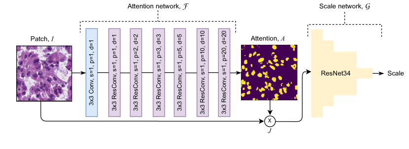
Figure 1: A diagram of our approach. Each patch $I$ is fed to the attention network $\mathcal{F}$ generating an attention map $A$. The “attended” image $J$ is then given to the scale classification network $\mathcal{G}$. Both networks are trained in an end-to-end fashion. s, p, and d for convolution blocks refer to stride, padding, and dilation.

3 Methodology

The main idea behind our approach is that given a patch extracted from a WSI viewed at a certain magnification, the level of magnification can be ascertained by looking at the size and texture of the nuclei in the patch. By extension, we further assume that the nuclei are enough to determine the level of magnification, and other artefacts in the image are not necessary for this task.

Contrary to several concurrent computer vision pipelines which propose to train and evaluate models by feeding images sampled at several scales in order for them to learn multi-scale features [9] or models which specifically train for scale equivariance [23], we posit learning a scale-sensitive network which specifically trains for discriminative features for correct scale classification. Given a set of WSIs, we extract all tissue patches (tiles) from them at a fixed set of magnifications $\mathcal{C}$. We consider only these tiles, with the “ground-truth” knowledge for each tile being at what magnification level it was extracted. Following our earlier reasoning, if nuclei in a given tile $I\in\mathbb{R}^{3\times H\times W}$ are enough to predict the level of magnification, we assume that there exists a corresponding attention map $A$, so that $A\odot I$ is also enough to determine the magnification, where $\odot$ represents element-wise multiplication, and $A\in[0,1]^{1\times H\times W}$ is a single channel attention image that focuses on the nuclei in the input tile (Figure 1).

We design a fully-convolutional feature extractor $\mathcal{F}$ to predict the attention map $A$ from the patch $I$. Our feature extractor consists of several layers of convolution operations with a gradual increase in the dilation of the kernels so as to incorporate information from a large neighborhood around every pixel. This feature extractor $\mathcal{F}$ regresses a confidence map $\mathbf{a}=\mathcal{F}\left(I\right)\in\mathbb{R}^{1\times H\times W}\,,$ which is activated by a compressed and biased sigmoid function so that $A=\sigma\left(\mathbf{a}\right)$. In order to force the attention map to focus only on parts of the input patch, we apply a sparsity regularizer on $A$. This regularizer follows the idea and implementation of a concurrent work on unsupervised separation of nuclei and background [10]. Sparsity is imposed by picking the $\eta$-th percentile value in the confidence map $\mathbf{a}$ for all images in the batch, and choosing a threshold $\tau$ equal to the average of this percentile over an entire training batch. Formally,

$$\tau=\frac{1}{B}\sum_{b=1}^{B}\mathbf{a}_{b}^{(\eta)}\,,$$ (1)

where $\mathbf{a}_{b}^{(\eta)}$ represents the $\left(\frac{\eta}{100}\cdot HW\right)$-th largest value in the confidence map $\mathbf{a}_{b}$ for the $b$-th image in the training batch of $B$ images. The sigmoid is then defined as $\sigma(x)=\frac{1}{1+\exp\left(-r\left(x-\tau\right)\right)}\,.$ It is compressed in order to force sharp transitions in the activated attention map, the compression being determined by $r$. We use $r=20$ in our experiments.

The “attended” image $J=A\odot I$ is now enough for magnification or scale classification. We train a scale classification network $\mathcal{G}$, which we initialize as a ResNet-34 [9], to predict the magnification level for each input tile $J$. The output of this network is scores for each magnification level, which is converted to probabilities using a softmax activation. The resulting model (Figure 1) is trainable in an end-to-end manner. We use negative log-likelihood to train the scale classification network $\mathcal{G}$, and in turn the attention network $\mathcal{F}$—

$$\mathcal{L}_{\mathrm{scale}}\left(\hat{\mathbf{p}},l\right)=-\log\hat{p}_{l}\,;\text{~{}}\hat{p}_{i}=\left[\mathrm{softmax}\left(\hat{\mathbf{s}}\right)\right]_{i}\,;\text{~{}}\hat{\mathbf{s}}=\mathcal{G}\left(J\right)\,;\text{~{}}\,1\leq i\leq N_{\mathcal{C}}\,,$$ (2)

where $l$ is the scale ground-truth, and $N_{\mathcal{C}}=\left|\mathcal{C}\right|\,.$

3.1 Smoothness Regularization

We wish $A$ to be semantically meaningful and smooth with blobs focusing on nuclei instead of having high frequency components. To this end, we incorporate a smoothness regularizer on the attention maps. The smoothness regularizer attempts simply to reduce the high frequency component that might appear in the attention map because of the compressed sigmoid. We employ a standard smoothness regularizer based on spatial gradients defined as

$$\mathcal{L}_{\mathrm{smooth}}=\frac{1}{(H-1)(W-1)}\sum_{i,j}\left\lVert A_{i+1,j}-A_{i,j}\right\rVert_{1}+\left\lVert A_{i,j+1}-A_{i,j}\right\rVert_{1}\,.$$ (3)

3.2 Transformation Equivariance

Equivariance is a commonly used constraint on feature extractors for imposing semantic consistency [22, 3]. A feature extractor $f$ is equivariant to a transformation $g$ if $g$ is replicated in the feature vector produced by $f\,,$ i.e., $f(g(\mathbf{x}))=g(f(\mathbf{x}))\,,$ for an image $\mathbf{x}$. In the given context, we want the attention map obtained from $\mathcal{F}$ to be equivariant to a set $\mathcal{T}$ of certain rigid transforms. We impose equivariance to these transformations through a simple mean squared error loss on $A$. Formally, we define the equivariance constraint as

$$\mathcal{L}_{\mathrm{equiv}}=\frac{1}{HW}\left\lVert\sigma\left(t\left(\mathcal{F}\left(I\right)\right)\right)-\sigma\left(\mathcal{F}\left(t\left(I\right)\right)\right)\right\rVert_{2}^{2}\,,$$ (4)

for a transformation $t\in\mathcal{T}$. We set $\mathcal{T}$ to include horizontal and vertical flips, matrix transpose, and rotations by $90$, $180$, and $270$ degrees.Each training batch uses a random $t\in\mathcal{T}\,.$

3.3 Training

The overall model is trained in an end-to-end fashion, with $\mathcal{L}_{\mathrm{scale}}$ being the guiding self-supervision loss. For models incorporating all constraints, i.e., smoothness, sparsity, and equivariance, the total loss is

$$\mathcal{L}_{\mathrm{total}}=\mathcal{L}_{\mathrm{scale}}+\mathcal{L}_{\mathrm{smooth}}+\mathcal{L}_{\mathrm{equiv}}\,.$$ (5)

We refer to a model trained with all these components together as $\mathsf{M}_{\mathrm{proposed}}$. We also test models without one of these losses to demonstrate how each loss contributes to the learning. More specifically, we define the following models:

1. $\mathsf{M}_{\mathrm{\lnot{}smooth}}$: does not include $\mathcal{L}_{\mathrm{smooth}}$.

2. $\mathsf{M}_{\mathrm{\lnot{}equiv}}$: does not include $\mathcal{L}_{\mathrm{equiv}}$.

3. $\mathsf{M}_{\mathrm{\lnot{}sparse}}$: does not include a sparsity regularizer on the attention map. In this case, the sigmoid is simply defined as $\sigma(x)=\frac{1}{1+\exp(-x)}\,$.

4. $\mathsf{M}_{\mathrm{\lnot{}WSI}}$: a model which does not sample images from WSIs, but instead from a set of pre-extracted patches (see Section 4.1).

We set the sparsity parameter $\eta$ empirically in order to choose the $93$-rd percentile value for sparsity regularization. This is equivalent to assuming that, on an average, $7\%$ of the pixels in a tile represent nuclei.

3.4 Post Processing, Validation, and Model Selection

In order to retrieve the final instance segmentation from the attention image we employ a post processing pipeline that consists of 3 consequent steps. Firstly, two binary opening and closing morphological operations are sequentially performed using a coarse and a fine circular element ($r=2$, $r=1$). Next, the distance transform is calculated and smoothed using a Gaussian blur ($\sigma=1$) on the new attention image and the local maxima are identified in a circular window ($r=7$). Lastly, a marker driven watershed algorithm is applied using the inverse of the distance transform and the local maxima as markers.

As our model does not explicitly train for segmentation of nuclei, we require a validation set to determine which model is finally best-suited for our objective. To this end, we record the Dice score between the attention map and the ground truth on the validation set (see Section 4.1) at intermediate training epochs, and choose the epoch which performs the best. We noticed that, in general, performance increases initially on the validation, but flattens after $\mathtt{\sim}30$ epochs.

4 Experimental Setup and Results

4.1 Dataset

For the purposes of this study we used the MoNuSeg database [13]. This dataset contains thirty $1000\times 1000$ annotated patches extracted from thirty WSIs from different patients suffering from different cancer types from The Cancer Genomic Atlas (TCGA). We downloaded the WSIs corresponding to patients included in the training split and extracted tiles of size $224\times 224$ from three different magnifications, namely $10\times\,$, $20\times\,$, and $40\times\,$. For each extracted tile, we perform a simple thresholding in the HSV color space to determine whether the tile contains tissue or not. Tiles with less then $70\%$ tissue cover are not used. Furthermore, a stain normalization step was performed using the color transfer approach described in [19]. Finally, a total of $1\,125\,737$ tiles from the three aforementioned scales were selected and paired with the corresponding magnification level. The MoNuSeg train and test splits were employed, while the MoNuSeg train set was further split into training and validation as $19$ and $11$ examples, respectively. The annotations provided by MoNuSeg on the validation set were utilized for determining the four post processing parameters (Section 3.4) and for the final evaluation. For the model $\mathsf{M}_{\mathrm{\lnot{}WSI}}$, which does not use whole slide images, we use the MoNuSeg patches instead for training, using the same strategy to split training and validation. We further evaluated the performance of our model that was trained on the MoNuSeg training set on the TNBC[15] and CoNSeP[7] datasets.

4.2 Implementation

We use the PyTorch [16] library for our code. We use the Adam [11] optimizer in all our experiments, with an initial learning rate of $0.0002\,$, a weight decay of $0.0001\,$, and $\beta_{1}=0.9\,$. We use a batch size of $32\,$, $100$ minibatches per epoch, and randomly crop patches of size $160\times 160$ from training images to use as inputs to our models. Furthermore, as there is a high imbalance among the number of tiles for each of the magnification level (images are about $4$ times more in number for a one step increase in the magnification level), we force a per-batch sampling of images that is uniform over the magnification levels, i.e., each training batch is sampled so that images are divided equally over the magnification levels. This is important to prevent learning a biased model.

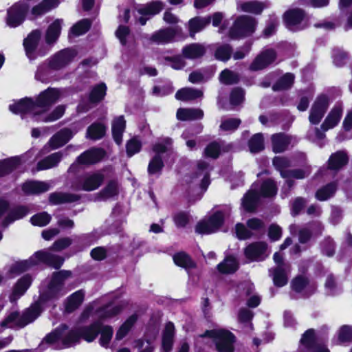
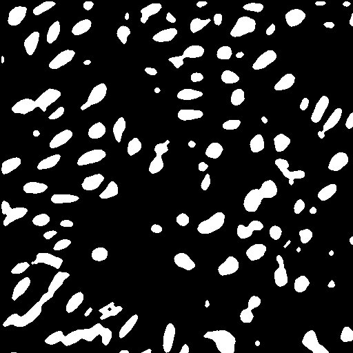
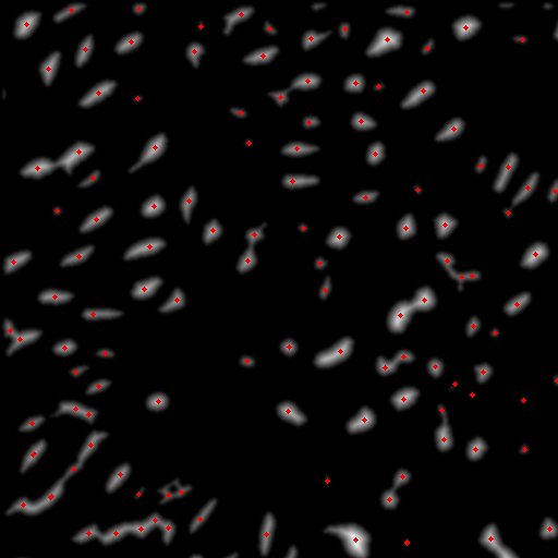
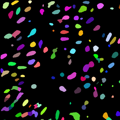
Figure 2: Input, intermediate results and output of the post processing pipeline. From left to right: the input image; the attention map obtained from $\mathsf{M}_{\mathrm{proposed}}$ after the post-processing; the distance transform together with local maxima over-imposed in red; and the final result after the marker driven watershed.

Test dataset	Method	AJI [13]	AHD	ADC
MoNuSeg test	CNN2 [13]†	0.3482	8.6924	0.6928
	CNN3 [13]†	0.5083	7.6615	0.7623
	Best Supervised [13]†	0.691	-	-
	CellProfiler [13]	0.1232	9.2771	0.5974
	Fiji [13]	0.2733	8.9507	0.6493
	$\mathsf{M}_{\mathrm{\lnot{}sparse}}$	0.0312	13.1415	0.2283
	$\mathsf{M}_{\mathrm{\lnot{}smooth}}$	0.1929	8.8166	0.4789
	$\mathsf{M}_{\mathrm{\lnot{}WSI}}$	0.3025	8.2853	0.6209
	$\mathsf{M}_{\mathrm{\lnot{}equiv}}$	0.4938	8.0091	0.7136
	$\mathsf{M}_{\mathrm{proposed}}$	0.5354	7.7502	0.7477
TNBC[15]	U-Net[7]†	0.514	-	0.681
	SegNet+WS[7]†	0.559	-	0.758
	HoverNet[7]†	0.590	-	0.749
	CellProfiler	0.2080	-	0.4157
	$\mathsf{M}_{\mathrm{proposed}}$	0.2656	-	0.5139
CoNSeP[7]	SegNet[7]†	0.194	-	0.796
	U-Net[7]†	0.482	-	0.724
	CellProfiler[7]	0.202	-	0.434
	QuPath[7]	0.249	-	0.588
	$\mathsf{M}_{\mathrm{proposed}}$	0.1980	-	0.587

Table 1: Quantitative results of the different benchmarked methods on three different public available datasets. AJI, AHD, and ADC stand for Aggregated Jaccard Index, Average Hausdorff Distance, and Average Dice Coefficient, respectively. Methods marked with ^† are supervised.

4.3 Results

To highlight the potentials of our method we compare its performance with supervised and unsupervised methods on the MoNuSeg testset presented in [13]. In particular, in Table 1 we summarize the performance of three supervised methods (CNN2,CNN3 and Best Supervised) and two completely unsupervised methods (Fiji and CellProfiler) together with different variations of our proposed method. Our method outperforms the unsupervised methods, and it reports similar performance with CNN2[13] and CNN3[13] on the same dataset. While it reports lower performance than the best supervised method from [13], our formulation is quite modular and able to adapt multi-task schemes similar to the one adapted by the winning method of [13].

On the TNBC and CoNSeP datasets, our method is strongly competitive among the unsupervised methods. We should emphasize that these results have been obtained without retraining on these datasets. The CoNSeP dataset consists mainly of colorectal adenocarcinoma which is under-represented in the training set of MoNuSeg, proving very good generalization of our method.

Moreover, from our ablation study (Table 1), it is clear that all components of the proposed model are essential. Sparsity is the most important as by removing it, the network regresses an attention map that is too smooth and not necessarily concentrating on nuclei, thus being semantically meaningless. Qualitatively, we observed that $\mathcal{L}_{\mathrm{smooth}}$ allows the network to focus on only on nuclei by removing attention over adjacent tissue regions, while $\mathcal{L}_{\mathrm{equiv}}$ further refines the attention maps by imposing geometric symmetry. Finally, in Figure 2 the segmentation map for one test image is presented. Results obtained from the $\mathsf{M}_{\mathrm{proposed}}$ attention network together with the nuclei segmentation after the performed post-processing are summarised.

5 Conclusion

In this paper, we propose and investigate a self-supervised method for nuclei segmentation of multi-organ histopathological images. In particular, we propose the use of the scale classification as a guiding self-supervision signal to train an attention network. We propose regularizers in order to regress attention maps that are semantically meaningful. Promising results comparable with supervised methods tested on the publicly available MoNuSeg dataset indicate the potentials of our method. We show also via. experiments on TNBC and ConSeP that our model generalizes well on new datasets. In the future, we aim to investigate the integration of our results within a treatment selection strategy. Nuclei presence is often a strong bio-marker as it concerns emerging cancer treatments (immunotherapy). Therefore, the end-to-end integration coupling histopathology and treatment outcomes could lead to prognostic tools as it concerns treatment response. Parallelly, other domains in medical imaging share concept similarities with the proposed concept.

References

- [1] Andrion, A., Magnani, C., Betta, P., Donna, A., Mollo, F., Scelsi, M., Bernardi, P., Botta, M., Terracini, B.: Malignant mesothelioma of the pleura: interobserver variability. Journal of clinical pathology 48(9), 856–860 (1995)
- [2] Boyle, D.P., McArt, D.G., Irwin, G., Wilhelm-Benartzi, C.S., Lioe, T.F., Sebastian, E., McQuaid, S., Hamilton, P.W., James, J.A., Mullan, P.B., et al.: The prognostic significance of the aberrant extremes of p53 immunophenotypes in breast cancer. Histopathology 65(3), 340–352 (2014)
- [3] Cohen, T.S., Weiler, M., Kicanaoglu, B., Welling, M.: Gauge equivariant convolutional networks and the icosahedral cnn. arXiv preprint arXiv:1902.04615 (2019)
- [4] Gamper, J., Alemi Koohbanani, N., Benet, K., Khuram, A., Rajpoot, N.: Pannuke: An open pan-cancer histology dataset for nuclei instance segmentation and classification. In: Digital Pathology. Springer International Publishing, Cham (2019)
- [5] Gidaris, S., Singh, P., Komodakis, N.: Unsupervised representation learning by predicting image rotations. arXiv preprint arXiv:1803.07728 (2018)
- [6] Gleason, D.F.: Histologic grading of prostate cancer: a perspective. Human pathology 23(3), 273–279 (1992)
- [7] Graham, S., Vu, Q.D., Raza, S.E.A., Azam, A., Tsang, Y.W., Kwak, J.T., Rajpoot, N.: Hover-net: Simultaneous segmentation and classification of nuclei in multi-tissue histology images. Medical Image Analysis 58, 101563 (2019)
- [8] Gurcan, M.N., Boucheron, L.E., Can, A., Madabhushi, A., Rajpoot, N.M., Yener, B.: Histopathological image analysis: A review. IEEE reviews in biomedical engineering 2, 147–171 (2009)
- [9] He, K., Zhang, X., Ren, S., Sun, J.: Deep residual learning for image recognition. In: Proceedings of the IEEE conference on computer vision and pattern recognition. pp. 770–778 (2016)
- [10] Hou, L., Nguyen, V., Kanevsky, A.B., Samaras, D., Kurc, T.M., Zhao, T., Gupta, R.R., Gao, Y., et al.: Sparse autoencoder for unsupervised nucleus detection and representation in histopathology images. Pattern recognition 86 (2019)
- [11] Kingma, D.P., Ba, J.: Adam: A method for stochastic optimization. arXiv preprint arXiv:1412.6980 (2014)
- [12] Kong, H., Gurcan, M., Belkacem-Boussaid, K.: Partitioning histopathological images: an integrated framework for supervised color-texture segmentation and cell splitting. IEEE transactions on medical imaging 30(9), 1661–1677 (2011)
- [13] Kumar, N., Verma, R., Sharma, S., Bhargava, S., Vahadane, A., Sethi, A.: A dataset and a technique for generalized nuclear segmentation for computational pathology. IEEE transactions on medical imaging 36(7), 1550–1560 (2017)
- [14] Long, J., Shelhamer, E., Darrell, T.: Fully convolutional networks for semantic segmentation. In: Proceedings of the IEEE conference on computer vision and pattern recognition. pp. 3431–3440 (2015)
- [15] Naylor, P., Laé, M., Reyal, F., Walter, T.: Segmentation of nuclei in histopathology images by deep regression of the distance map. IEEE transactions on medical imaging 38(2), 448–459 (2018)
- [16] Paszke, A., Gross, S., Chintala, S., Chanan, G., Yang, E., DeVito, Z., Lin, Z., Desmaison, A., Antiga, L., Lerer, A.: Automatic differentiation in pytorch (2017)
- [17] Pathak, D., Agrawal, P., Efros, A.A., Darrell, T.: Curiosity-driven exploration by self-supervised prediction. In: Proceedings of the IEEE Conference on Computer Vision and Pattern Recognition Workshops. pp. 16–17 (2017)
- [18] Plissiti, M.E., Nikou, C.: Overlapping cell nuclei segmentation using a spatially adaptive active physical model. IEEE Transactions on Image Processing 21(11) (2012)
- [19] Reinhard, E., Adhikhmin, M., Gooch, B., Shirley, P.: Color transfer between images. IEEE Computer graphics and applications 21(5), 34–41 (2001)
- [20] Ruan, M., Tian, T., Rao, J., Xu, X., Yu, B., Yang, W., Shui, R.: Predictive value of tumor-infiltrating lymphocytes to pathological complete response in neoadjuvant treated triple-negative breast cancers. Diagnostic pathology 13(1), 66 (2018)
- [21] Rubin, R., Strayer, D.S., Rubin, E., et al.: Rubin’s pathology: clinicopathologic foundations of medicine. Lippincott Williams & Wilkins (2008)
- [22] Thewlis, J., Bilen, H., Vedaldi, A.: Unsupervised learning of object landmarks by factorized spatial embeddings. In: Proceedings of the IEEE International Conference on Computer Vision. pp. 5916–5925 (2017)
- [23] Worrall, D., Welling, M.: Deep scale-spaces: Equivariance over scale. In: Advances in Neural Information Processing Systems (2019)
- [24] Yi, F., Huang, J., Yang, L., Xie, Y., Xiao, G.: Automatic extraction of cell nuclei from H&E-stained histopathological images. Journal of Medical Imaging 4(2) (2017)